estimation and testing for fractional cointegration - core · estimation and testing for fractional...

Estimation and Testing for Fractional Cointegration

Marcel Aloy, Gilles De Truchis

To cite this version:

Marcel Aloy, Gilles De Truchis. Estimation and Testing for Fractional Cointegration. 2012.<halshs-00793206>

HAL Id: halshs-00793206

https://halshs.archives-ouvertes.fr/halshs-00793206

Submitted on 21 Feb 2013

HAL is a multi-disciplinary open accessarchive for the deposit and dissemination of sci-entific research documents, whether they are pub-lished or not. The documents may come fromteaching and research institutions in France orabroad, or from public or private research centers.

L’archive ouverte pluridisciplinaire HAL, estdestinee au depot et a la diffusion de documentsscientifiques de niveau recherche, publies ou non,emanant des etablissements d’enseignement et derecherche francais ou etrangers, des laboratoirespublics ou prives.

https://hal.archives-ouvertes.fr

https://halshs.archives-ouvertes.fr/halshs-00793206

Working Papers / Documents de travail

WP 2012 - Nr 15


Marcel AloyGilles de Truchis


Marcel Aloy ∗ and Gilles de Truchis †

June 5, 2012

Abstract

Estimation of bivariate fractionally cointegrated models usually operates in two steps:the first step is to estimate the long run coefficient (β) whereas the second step estimatesthe long memory parameter (d) of the cointegrating residuals. We suggest an adaptationof the maximum likelihood estimator of Hualde and Robinson (2007) to estimate jointly βand d, and possibly other nuisance parameters, for a wide range of integration orders whenregressors are I(1). The finite sample properties of this estimator are compared with vari-ous popular estimation methods of parameters β (LSE, ADL, DOLS, FMLS, GLS, MLE,NBLS, FMNBLS), and d (LPE,LWE,LPM,FML) through a Monte Carlo experiment. Wealso investigate the crucial question of testing for fractional cointegration (that is, d < 1).The simulation results suggest that the one-step methodology generally outperforms othersmethods, both in terms of estimation precision and reliability of statistical inferences. Fi-nally we apply this methodology by studying the long-run relationship between stock pricesand dividends in the US case.

JEL classification: C32, C15, C53, C58.Keywords: Fractional cointegration; Long memory; Monte Carlo experiment; Cointegrationtest.

1 INTRODUCTION

This paper deals with estimation of a generalized form of the standard triangular cointegra-tion model:

(1 − L)d(yt − βxt) = ε1t, (1 − L)δxt = ε2t, t = 1, ..., n (1)

In equation (1), we assume that εt = [ε1t, ε2t]> is a vector of I(0) variables, ωt = [yt, xt] a vectorof I(δ) variables and we define (1 − L)d by its binomial expansion

∗Corresponding author. Aix-Marseille School of Economics, Aix-Marseille University, Chateau La Farge, Routedes Milles, 13290 Aix-en-Provence, France ([email protected])

†Aix-Marseille School of Economics, Aix-Marseille University, 13290 Aix-en-Provence, France ([email protected])

1

(1 − L)d = 1 − dL −d(1 − d)

2!L2 −

d(1 − d)(2 − d)3!

L3 − ...

=

+∞∑k=0

Γ(k − d)Γ(k + 1)Γ(−d)

Lk (2)

Γ(z) =

∫ +∞

0tz−1e−tdt,

where L is the lag operator and (1−L)d the fractional difference operator (denoted ∆d). Equation(1) extends the traditional cointegration framework since we allow d ∈ (0, 1) and δ ∈ (0, 1) to bereal numbers, while d = 0 and δ = 1 corresponds to the standard cointegration model. Accordingto Granger (1986) and Engle and Granger (1987), cointegration arises when d < δ. The casewhere d < δ implies a dimensionality reduction, revealing a near-zero-frequency correlationbetween the two series. Denoting λ = δ−d the reduction parameter and C(δ, λ) the cointegrationrelationship we can identify five cases:

i) strong fractional cointegration C(δ, λ): 1/2 < δ ≤ 1, 0 ≤ d < 1/2 and λ > 1/2;

ii) weak fractional cointegration C(δ, λ): 0 < δ ≤ 1, 0 < d < δ and λ < 1/2;

iii) stationary fractional cointegration C(δ, λ): 0 < δ < 1/2, 0 ≤ d < δ and λ < 1/2;

iv) standard cointegration C(1, 1): δ = 1, d = 0 and λ = 1;

v) spurious regression: 1/2 ≤ δ ≤ 1, 1/2 ≤ d ≤ δ and λ = 0.

The concepts of stationary and weak fractional cointegration result from properties of fraction-ally integrated process demonstrated by Granger and Joyeux (1980) and Hosking (1981): anI(d) process is covariance stationary when d < 0.5 and covariance non-stationary when d ≥ 0.5.As long a d < 1 the process is mean reverting. Consequently , in equation (1), d < δ ≤ 1 impliesthe existence of a reversion mechanism toward the long run equilibrium.

In the standard cointegration framework the long run coefficient β is the only parameter ofinterest and the literature provides many studies dealing with estimation of β in this specific case.Panopoulou and Pittis (2004) lead a finite sample comparison of the most commonly used esti-mators. In the more general case of fractional cointegration, parameters of interest in equation(1) are β, d and δ. Consequently, the joint estimation of parameters in equation (1) is tediousand existing studies focuse on only specific cases. The seminal paper of Cheung and Lai (1993)suggests a two-step methodology carrying out the Least Squares Estimator (LSE) and the Log-Periodogram regression Estimator (LPE) of d, developed by Geweke and Porter-Hudak (1983).It consists in estimating β in a first step and d, upon collected residuals, in a second step. Theirapproach cover the fractional cointegration case but they restrict δ = 1. Marinucci and Robinson (2001)provide a good overview of fractional cointegration and investigate asymptotic and finite sampleproperties of the Narrow-Band Least Squares estimator of β (introduced by Robinson (1994))for different parameter regions. Nielsen (2007) suggests a quasi-maximum likelihood estimatorin order to estimate jointly β, d and δ. This local Whittle estimator operates in frequency domain

2

and is consistent and asymptotically normal for the entire stationary region of δ and d (so it isrestricted to the stationary fractional cointegration case). Finally, Hualde and Robinson (2007)present a time domain maximum likelihood estimator of β, d and δ. Hualde and Robinson (2007)demonstrate consistency and asymptotic normality of this estimator under assumptions of weakfractional cointegration. However their methodology operates in two non-linear optimizations.

The aim of this paper is to analyse various estimation strategies of bivariate fractional coin-tegration models under the restriction δ = 1. This specific restriction is relevant to a widerange of financial and macroeconomics applications. For instance, Cheung and Lai (1993) bringout some evidence of cointegration at orders C(1, 0.4) exploring the purchasing power par-ity relationship between United States and United Kingdom (see Henry and Zaffaroni (2003)for a survey of applications in macroeconomics and finance in presence of long-memory).Marinucci and Robinson (2001) analyze the consumption and the GNP in the U.S. case andfind them integrated at order 1. However, they get inconclusive results concerning the inte-gration order of cointegrating errors. Caporale and Gil-Alana (2002) test the cointegration hy-pothesis between unemployment and input prices and find some evidence of cointegration atorder C(1, λ), where λ depends on the residuals specification (AR(1), AR(2) or white noise).Baillie and Bollerslev (1994) investigate dynamic relationships between different exchange rateseries and conclude to cointegration at orders C(1, 0.11). Using the same times series, Nielsen (2004)tests the C(1, 1) cointegration hypothesis against the alternative of fractional cointegration. Thispaper leads up to the crucial question of testing cointegration that constitutes our second pointof interest. Cheung and Lai (1993) provide a finite sample analysis of a fractional cointegrationtest based upon the log-periodogram estimator. The empirical distribution of their test statisticunder the null appears to be negatively skewed. As a consequence this cointegration test rejectsthe null hypothesis of no cointegration too often. Lobato and Velasco (2007) develop a frac-tional Wald test of fractional integration and suggest that this test can also be applied for testingfractional cointegration. Since they provide neither asymptotic nor finite sample properties oftheir test in the case of fractional cointegration, we include it in our simulations.

Under the assumption δ = 1, there are two free parameter of interest: d and β. In the two-stepmethodology initiated by Cheung and Lai (1993), there is a wide range of candidate to estimated. The main drawback of the semi-parametric frequency approach of Geweke and Porter-Hudak (1983)used by Cheung and Lai (1993) is a negative bias in small sample. Andrews and Guggenberger (2003)suggest a Log-Periodogram (LPM) Modified estimator in order to correct the bias. In com-parison with the LPE and the LPM, the Local Whittle semi-parametric Estimator (LWE) ofKunsch (1987) and Robinson (1995) has convenient asymptotic properties, but requires a numer-ical optimization. In a different spirit, a parametric frequency maximum likelihood (FML) ap-proach is proposed by Fox and Taqqu (1986). Finally, we can can also mention the time domainmaximum likelihood estimator of Sowell (1992). An exhaustive list of fractional integration esti-mator is considered in the Monte-Carlo experiment performed by Nielsen and Frederiksen (2005).Estimators we have mentioned above exhibit best finite sample properties according to theirstudy (except Sowell (1992)).

The second parameter of interest is β. In the standard cointegration case, Stock (1987)demonstrates that the LSE is still consistent but super-convergent at the rate O(n) rather thanthe optimal rate O(n1/2). It implies that the LSE will be biased in small sample. This result is

3

extended by Robinson and Marinucci (2001) to the fractional cointegration case: when δ = 1,it can be shown that the LSE converges at the rate nλ for λ > 1/2, (n/ log(n))1/2 for λ = 1/2,and n1/2 for 0 < λ < 1/2. Hence, it easy to recover the standard results, for instance thespurious regression case when λ = 0, and the traditional cointegration case when λ = 1. Asecond issue is the inconsistency of the LSE estimator of β when cointegrating errors and re-gressors both have long memory and have non-zero coherence at the zero frequency. Considerthe equation yt = βxt + υt. One sufficient condition of consistency of the LSE estimator of β isthat

∑nt=1 υ

2t /

∑nt=1 x2

t converges stochastically to zero when n → ∞. This condition is satisfiedwhen δ > 1/2 and d < 1/2, ore more generally when the residuals are ”less nonstationary”than yt and xt (Robinson and Marinucci (2001)). However, the LSE are generally inconsis-tent when xt and υt are correlated and d < δ < 1/2: in this case,

∑nt=1 x2

t does not dominate∑nt=1 υ

2t . Focusing on the stationary case, Robinson (1994) has developed a semi-parametric

Narrow-Band Least Squares estimator (NBLS) in the frequency domain. NBLS exploits thedominance of the spectral density of xt on υt at low frequencies (since cointegration impliesδ > d). However the NBLS estimator is confined to the case δ < 1/2 (where yt, xt and zt havefinite variances) and in practice it is difficult to ensure that we are in the stationary regions ofδ. In order to solve this drawback, Nielsen and Frederiksen (2011) suggest a Fully ModifiedNarrow-Band Least Squares (FMNBLS) to take into account bias that appears in the limitingdistribution of the NBLS in presence of a non-zero long run coherence between regressors andcointegrating errors, in the weak fractional cointegration case (λ < 1/2). Their approach isequivalent to the so called time domain Fully-Modified Least Squares (FMLS) estimator ofPhillips and Hansen (1990). Panopoulou and Pittis (2004) propose to exploit an AutoregressiveDistributed Lags structure of the equation (1) to estimate β. They demonstrate the good finitesample properties of the LSE in the ADL form throughout simulations. They also investigatethe Dynamic Ordinary Least Squares of Stock and Watson (1993) and show this estimator sufferfrom truncation bias in finite sample. An other candidate to estimate β is the time domain Gener-alized Least Squares (GLS) estimator. A frequency domain version of this parametric estimatoris given by Robinson and Hidalgo (1997): they demonstrate root-n-consistency and asymptoticnormality of this estimator when the true specification of errors is known. More recently, theyadapt it to unknown specification of disturbance (see Hidalgo and Robinson (2002)). Finally, wecan mention the well-known Maximum Likelihood Estimator (MLE) of Johansen (1988): sincethis estimator is not designed to estimate fractional cointegrated models, we can expect mixedresults in non-stationary regions of cointegrating errors.

All estimators presented above are relevant either in estimation of β or in estimation of d.In the spirit of Nielsen (2007) and Hualde and Robinson (2007) we are interested in the jointestimation of parameters of interest, which are limited to β and d since we assume δ = 1.We are also interested in estimating those parameters for a wide range of integration orders.Since we adopt a parametric approach, we cannot avoid issues of serial correlation and the lackof orthogonality between errors and regressors. In consequence, we suggest an adaptation ofthe model of Hualde and Robinson (2007) that is still relevant with the Maximum LikelihoodEstimator (MLE). We also advise a selection procedure of the parametric form of this model.We investigate the finite sample properties of the MLE of β and d. The question of testingcointegration is also performed using the asymptotic variance, derived by Tanaka (1999), in the

4

framework of a Wald test. We compare our one step methodology with most of estimatorsmentioned previously. The outline of the paper is as follows. The section 2 presents sometechnical aspects of the fractional cointegration framework and the model we consider, and thendetails various estimators used in our simulation. In the section 3 we comment our simulationsand the results. We finally lead an empirical study on the present value model in the section 4.The section 5 concludes.

2 SIMULATION DESIGN

2.1 The fractional cointegration model

We consider now a generalized form of equation (1) that allows for serial correlation of errorsand weak exogeneity of regressors. Let ωt and ζt be two bivariate processes where ωt = [yt, xt]>

is a vector of I(1) variables and ζt = [υt, zt]> a vector of their residuals. We assume that[∆dυt, zt]> is a two dimensional vector of I(0) variables with a VAR(1) structure driven byεt = [ε1t, ε2t]> and the data generating process (DGP) for yt is given by the following system,

yt = βxt + υt (3)

xt = xt−1 + zt (4)

((1 − L)dυt

zt

)=

(α11 α12α21 α22

) ((1 − L)dυt−1

zt−1

)+

(ε1,tε2,t

)(5)

(ε1t

ε2t

)∼ i.i.d N

[(00

),

(σ11 σ12σ21 σ22

)](6)

Our analysis will be restricted to the case where α21 = α12 = α22 = 0: if the two last re-strictions are only simplifying assumptions, the first one (α21=0) is crucial as it insures that xt

is weakly exogenous for β, since xt does not adjust to past cointegration errors. In the standardI(1)/I(0) framework, Johansen (1992) shows that under weak exogeneity of xt, the single equa-tion modelling is equivalent to the ML estimation of the full system. We assume further thateigenvalues of the matrix A=[αi j], i, j = 1, 2 are less than one in modulus: under the restric-tion α21 = 0, this hypothesis implies α11 < 1 (and α22 < 1 if one would relax our simplifyingassumption α22 = 0).

The contemporaneous correlation between the elements of et leads us to suggest a triangularrepresentation in which we assume

ε1t = αε2t + εt (7)

where,

α = σ12/σ22, V(ε) = σ11 − (σ212/σ22) = σ2

ε, εt ∼ i.i.d N(0, σ2ε)

The process for the cointegration errors can thus be written more compactly as it follows

5

∆dυt = α11∆dυt−1 + αε2t + εt (8)

Under our set of assumptions, it results that:- xt is a weakly exogenous I(1) process for β and follows a simple random walk;- assuming β , 0, xt and yt are two I(1) fractional cointegrated processes provided that d < 1.

These two processes are not cointegrated if d = 1, and are cointegrated under the usual I(1)/I(0)framework if d = 0;

- if xt and yt are two I(1) processes and are cointegrated under the I(1)/I(0) framework, thelong-run multiplier between xt and yt is given by the parameter β while the short-run multiplieris given by the sum β + α. It is thus important to consider the case where α , 0 since itcorresponds to a short-run undershooting (α < 0) or overshooting (α > 0) following a shock onxt. It is also important to consider the case where α11 , 0: if the two series are cointegratedunder the I(1)/I(0) framework, the cointegrating errors will follow a simple and unrealistic whitenoise if α11 = 0.

Restricting some coefficients of this model, we define four specifications which will be usedlater in our Monte Carlo study.

Table 1: Some parameters combinationsModel α α11 α12 α21 α22

A 0 0 0 0 0B1 0 > 0 0 0 0B2 < 0 0 0 0 0B3 < 0 > 0 0 0 0

The first model, denoted A, describes a bivariate relationship between yt and xt in line withCheung and Lai (1993). Indeed, innovations are a simple fractional white noise integrated atorder d while xt is defined as a random walk with drift. The model B1 corresponds to the casewhere α = 0 and α11 > 0: the cointegration residuals follows thus an ARFIMA(1,d,0) processwith a positive AR coefficient (since α11 > 0). Conversely, the model B2 corresponds to thecase of α11 = 0 and α < 0. In other terms, we introduce here the second order bias sinceα < 0 breaks the orthogonality condition: E[υt|xt] , 0. In the specifications B3, the modelfaces simultaneously serial correlation and engoneity in the cointegration residuals (α11 > 0 andα < 0) : innovations follow an ARFIMA(1,d,0) process with a positive AR coefficient and areadversely influenced by current shocks on xt (since α < 0).

2.2 Estimators

We will examine eight different estimators of the long run coefficient β: the ordinary leastsquares (LSE), the generalized least squares (GLS), the fully modified least squares (FMLS),the dynamic LSE (DOLS), the autoregressive distributed lags (ADL), the maximum likelihoodestimator (MLE) of Johansen (1988) (although the methodology of Johansen (1988) is clearlylimited to the standard I(1)/I(0) case, we considered that it was interesting to evaluate its perfor-

6

mances in the case of fractional cointegration), the narrow band least squares (NBLS) and thefully modified narrow band least squares (FMNBLS).

Concerning the fractional differencing parameter (d) of the cointegrating errors, we willconsider four estimators: the log-periodogram regression estimator (LPE), the modified log-periodogram estimator (LPM), the gaussian semi-parametric estimator (LWE) and the approx-imate Whittle Frequency domain Maximum Likelihood estimator (FML). Notice that these es-timators of d have not been developed to be applied to estimated residuals. Moreover, someof them are semi-parametric and thus we can expect some biases in presence of short run dy-namics in residuals. Alternatively, some of them are parametric and they potentially outper-form semi-parametric estimators, provided that we are able to select the true underlying datageneration process. In addition we suggest a parametric model, based on Tanaka (1999) andHualde and Robinson (2007), that allows to estimate simultaneously β and d. It clearly appearsas an alternative convenient way to address issues raised by the two-step methods. We denote itFCMLE.

2.2.1 Estimators of β

In the fractional cointegration case, the least squares estimates of the cointegrating parameter isconsistent and converge in probability at the rate O(nmin(2δ−1,λ)) (Robinson and Marinucci (2001)and Robinson and Hualde (2003)). Thus, the case where δ = 1 and λ = 1 corresponds to theI(1)/I(0) framework and we find back the convergence results demonstrated by Stock (1987).When δ = 1 and λ = 0, least squares estimates does not converge and the cointegrating regres-sion is spurious. Since we focus on the case δ = 1, we don’t cover the stationary case consideredby Robinson (1994).

The fractional cointegration framework we consider involves serially dependent errors andthus non-spherical disturbances. Therefore, least squares estimator is no longer efficient and aconvenient way to deal with this issue is to use GLS estimators. Since the covariance matrixΩυ is unknown, we can apply feasible GLS (FGLS). For instance, the Prais and Winsten (1954)method can be used to build the unknown covariance Ω(ς)υ, which is assumed to be dependentupon several unobservables parameters ς:

Ω−1υ (ς) =

1σ2υ

1 −α11 0 0 · · · 0−α11 1 + α2

11 −α11 0 · · · 00 −α11 1 + α2

11 −α11 · · · 0...

. . .. . .

...

0 · · · 0 −α11 1 + α211 −α11

0 · · · 0 0 −α11 1

The FGLS estimator of β is thus:

βGLS =

n∑t=1

xtΩ(ς)−1υ x>t

−1 n∑t=1

xtΩ(ς)−1υ yt

(9)

When α , 0, the orthogonality condition is no longer satisfied since Cov(υt|xt) , 0.Phillips and Hansen (1990) suggest a fully modify least square estimator (FMLS), applying non-

7

parametric corrections to the covariance matrix to take into account endogeneity and serial cor-relation. The FMLS estimator of β is given by

βFMLS =

n∑t=1

xt x>t

−1 n∑t=1

xt(yt − λ+) − T δ+

, (10)

where λ+ is the correction term associated with the correction for the endogeneity bias while δ+

eliminates the non-centrality bias. Assuming that the long-run variance of residuals is positivedefinite and can be expressed as Ω = Λ + Ξ> = Σ + Ξ + Ξ>, we can partition Ω and Λ such as

Ω =

(ω11 ω12ω21 Ω22

), Λ =

(λ11 λ12λ21 Λ22

),

where Σ = limn→∞

1/n∑n

t=1 E(υtυ>t ) and Ξ = lim

n→∞1/n

∑n−1j=1

∑n− jt=1 E(υtυ

>t+ j). It results that λ+ =

yt − ω12Ω−122 zt and δ+ = [0, λ21 − Λ22Ω−1

22 ω21]>, where zt refers to the error term of xt.Alternatively, Stock and Watson (1993) consider a parametric correction based upon an aug-

mented regression equation, in order to provide an estimator robust to endogeneity. The dynamicLSE (DOLS) estimator of β is

βDOLS =

n−k∑t=k+1

utu>t

−1 n−k∑

t=k+1

utyt

, (11)

where, ut = [1, x>t ]> and ut and yt are regression residuals of ut and yt on ζ2t = (z>t+k, ..., z>t−k)>,

respectively (for a detailed review of these estimators, see Kurozumi and Hayakawa (2009)).Johansen (1988) adopts a vectorial approach of the cointegration theory in a I(1)/I(0) frame-

work. Starting from the long run equation, the vectorial error correction model is

(1 − L)yt = µ + Πyt−1 +

p−1∑j=1

Θ j∆yt− j + vt

where yt = [yt, xt]> and vt is an k = 2 × 1 vector of innovations. This equation is clearly acombination of I(1) and I(0) variables. However, if the coefficient matrix Π has reduced rankr < k, then we can decompose Π as k × r matrix α and ξ such that Π = αξ>. It appears nowthat ξ>yt is stationary since ξ is the matrix of cointegrating vectors, while α is the matrix ofadjustment coefficients.

Let u1t be the residuals in the regressions of ∆yt on zt = ∆yt−1,∆yt−2, ...,∆yt−p+1 and u2t

the residuals in the regressions of yt−p on zt. With respect to parameters Θ1, ...,Θp−1, µ, themaximum likelihood function is the following,

⇒ L−2/nmax (r) = |S 00|

r∏j=1

(1 − λ j) (12)

where the eigenvalue λ j is the jth largest canonical correlation of (1 − L)yt with yt−1 after cor-recting for lag differences and S i j the cross-correlation matrix between variables in set i and set

8

j for i, j = u1t,u2t1. Notice that in a bivariate cointegration model, the Π matrix contains at most

one cointegrating vector.When λ = 1, the model defined by equations (3), (4), (5), and (6), can also be parametrized

as an autoregressive distributed lag (ADL) model (see Panopoulou and Pittis (2004)). Hence theconditional density of yt, with an ADL(1,1), can be expressed as

D(yt|xt, ωt−1, θ) = N(βxt + c1yt−1 + c2xt−1, σ2e), θ ≡ (c0, c1, c2, σ

2e),

with

β = β +σ12

σ22

c1 = α11 − α21σ12

σ22= α11

c2 = α12 − (α22 + 1 − α21β)σ12

σ22− α11β = −α11β

σ2u = σ11 −

σ212

σ22

Hence, the ADL equation is given by

yt = βxt + c1yt−1 + c2xt−1 + et, (13)

and the equation of β by

β =β + c2

1 − c1, (14)

where error term et in this ADL representation is orthogonal to zt. Panopoulou and Pittis (2004)show that the LSE of (13) can be employed to obtain an efficient estimator of β using (14).

In a seminal paper, Robinson (1994) provides a semi-parametric frequency domain narrow-band least squares (NBLS) estimator of β. Robinson (1994) restricts his analysis to the stationaryregion of δ and d, and deals with long-run non-zero coherence between υt and xt. Since weimpose δ = 1, our simulation is not theoretically relevant with this framework. However, weare still interested in the finite sample performance of the NBLS when δ ≥ 1/2. Assume anynon-negative real γ which transforms the following hypothetical model,

(1 − L)γyt = β(1 − L)γxt + (1 − L)γυt,

into a stationary model. In the special case investigated by Robinson (1994), γ = 0 since it isassumed that variables of the model are covariance stationary. Then, the NBLS estimator of β isdefined by:

βNBLS (m, γ) = F−1xx (γ, 1,m)Fxy(γ, 1,m), (15)

1Lasak (2010) suggests to extend the Johansen MLE estimator to fractional processes. However, we do notconsider this estimator since the asymptotic theory is still a work in progress.

9

where the average co-periodogram is

Fq,r(γ, k, l) =2πn

l∑j=k

Re(Iqr(γ, λ j)), 0 ≤ k ≤ l ≤ n − 1, (16)

and the co-periodogram is

Iq,r(γ, λ) =1

2πn

n∑t=1

n∑s=1

((1 − L)γqt)((1 − L)γrs)′e−i(t−s)λ (17)

Nielsen and Frederiksen (2011) extend the NBLS estimator to the case where γ > 0 (inthis case, the time series are covariance non-stationary) and propose a fully modified NBLS(FMNBLS) estimator in order to correct the bias that appears in presence of non-zero coherencebetween errors and regressors. The FMNBLS estimator of β is expressed as

βFMNBLS (m3, γ) = βNBLS (m3, γ) − λ−dm3λδm3

λdm2λ−δm2

Γm2(γ), (18)

where λ j is the angular frequency. The estimators of the bias is given by

Γ(m2, γ) = F−1xx (γ,m0 + 1,m2)Fxυ(γ,m0 + 1,m2), (19)

where the modified average co-periodogram Fq,r is

Fq,r(γ, k, l) =2πn

l∑j=k

Re(eiλ j(dq−dr)/2Iqr(γ, λ j)), 0 ≤ k ≤ l ≤ n − 1 (20)

Bandwidths can be chosen such as m0 = m3 = 0.3, m1 > 0.675 and m2 ∈ (0.675, 0.85), whenλmin = 0.4 (λ refers here to the reduction parameter).Nielsen and Frederiksen (2011) use the local Whittle estimator of Robinson (1995) to estimateδ with bandwidth m1. Nielsen and Frederiksen (2011) demonstrate the asymptotic normality ofthis estimator, albeit δ is estimated beforehand.

2.2.2 Estimators of d

In this section we review some estimators of d that we consider in the Monte Carlo study2. Fistwe recall some useful properties of long memory process. Let υt an autoregressive fractionallyintegrated moving average model, ARFIMA(p,d,q), defined by

Φ(L)(1 − L)dυt = Ψ(L)et, d ∈ (0, 1/2) (21)2The time domain exact maximum likelihood estimator (EML) of Sowell (1992) is not considered here. Ac-

cording to the Monte-Carlo study of Nielsen and Frederiksen (2005), finite sample performances of EML estimatorstrongly depend on specifications and has poor finite sample properties relatively to other parametric estimators likeFML. Notice also that Dubois et al. (2004) investigate the EML-based fractional cointegration test and point out thatthe power of this test decreases when the sample size increases. They also bring out that the size of this test stronglydepends on the short run coefficients and perform badly in some cases.

10

where

Φ(L) = 1 −p∑

j=1

φ jL j, Ψ(L) = 1 +

q∑j=1

ψ jL j,

are polynomials of orders p and q in the lag operator, with roots outside the unit circle.The autocorrelation function of the process in (21) decays at an hyperbolic rate (2d−1) and thussatisfies

ρk ∼ cρk2d−1, 0 < cρ < ∞, as k → ∞ (22)

The autocovariance function of υt is defined by,

γ(k) =1

2π

∫ π

−πfυ(λ)e−ikλdλ, π ≥ λ ≥ −π (23)

where fυ(λ) denotes the spectral density function of υt:

fυ(λ) =σ2

2π|1 − eiλ|−2d

∣∣∣∣∣∣Ψ(eiλ)Φ(eiλ)

∣∣∣∣∣∣2 , (24)

with λ j =2π jn the angular frequencies. Under some additional conditions it can be shown that

equation (22) is equivalent to the following approximation of (24), near zero frequency,

fυ(λ) ∼ g|λ|−2d, 0 < g < ∞, as k → 0 (25)

Exploiting those properties, Fox and Taqqu (1986) suggest a convenient parametric frequencymaximum likelihood estimator (FML) based upon the spectral density of υt and the log-periodogramI(λ),

I(λ) =1

2πT

∣∣∣∣∣∣∣n∑

t=1

υteitλ

∣∣∣∣∣∣∣2

, (26)

The Whittle form of the log-likelihood function they obtain is:

L(d,Φ,Ψ, σ2) = −

n/2∑j=1

[ln fy(λ j) +

I(λ j)fy(λ j)

], (27)

Assuming gaussianity and d ∈ −1/2, 1/2, the FML estimator verifies asymptotically

√n(dFML − d)→ N

(0,

4πΩ(ς)

),

where Ω(ς) is a p × p matrix, depending on unknown parameters ς and with j, kth entry suchthat,

ω j,k(ς) =

∫ π

−πf (υ, ς)

∂2

∂ς j∂ςkf −1(υ, ς)dυ

11

The so called log-periodogram least square regression (LPE) of Geweke and Porter-Hudak (1983)is one of the most commonly applied estimator. While such estimator does not depend on short-run dynamics parameters, it is less efficient since only

√m-consistency is achieved. From equa-

tion (25), Geweke and Porter-Hudak (1983) suggest to estimate the following equation using theLSE:

ln I(λ j) = c − d ln(4 sin2(λ j/2)) + e(λ j), j = 1, ...,m (28)

The bandwidth number for the log-periodogram is arbitrarily fixed to m =√

n. The LSE ofd ∈ (−1/2, 1/2) is asymptotically normally distributed such as:

√m(dLPE − d)→ N

(0,π2

24

)Andrews and Guggenberger (2003) investigate the bias source of the LPE estimator and sug-

gest to replace the constant term c in (28) by the polynomial∑R

r=0 cτλ2rj , leading to the new

regression model:

ln I(λ j) =

R∑r=0

cτλ2rj − d ln(4 sin2(λ j/2)) + ε, (29)

Thus, assuming that d ∈ −1/2, 1/2, the asymptotic distribution of this modified log-periodogramestimator (LPM) is

√m(dLPM − d)→ N

(0,π2

24cR

), cR=1 = 2.25, d ∈ −1/2, 1/2

Another semi-parametric approach is suggested by Kunsch (1987) using a local Whittle ap-proach and revisited by Robinson (1995). The Whittle form log-likelihood function of the localWhittle estimator (LWE) is defined as follows:

L(g, d) = −1m

m∑j=1

ln(gλ−2dj ) +

I(λ j)

gλ−2dj

, (30)

where gλ−2d corresponds to the approximation of the spectral density in (25). Robinson (1995)also demonstrates that the asymptotic distribution of the LWE is normal:

√m(dLWE − d)→ N (0, 1/4) , d ∈ −1/2, 1/2

Various others long memory estimators have been developed during the last three decades(see Nielsen and Frederiksen (2005) for a Monte Carlo comparison of numerous ARFIMA(p,d,q)estimators). However, we limit ourselves to the most diffused and efficient.

12

2.2.3 A simultaneous estimator of β and d

Most of the time, the two-step methodology (e.g. Cheung and Lai (1993)) uses semi-parametricmethods to estimate fractional integration parameters and parametric methods to estimate long-run parameters. This approach involves a loss of efficiency since the estimators are globally lessthan

√n-consistent. According to Hualde and Robinson (2007) these parameters ought to be

jointly estimated parametrically to achieve√

n-consistency and they advise to use the GaussianMaximum Likelihood Estimator in order to estimate δ, β and d. Outside the cointegration con-text, Tanaka (1999) proves that the time domain Gaussian maximum likelihood estimator of d isasymptotically efficient and normally distributed. He shows that

√n(d − d)→ N(0, 6/π2) when

υt is a fractional white noise, and that√

n(d−d)→ N(0, ω−2), where ω is detailed in (39), whenυt follows a process similar to (21). Moreover, Tanaka (1999) proposes a two-step parametriccointegration methodology based on the LSE of β and the MLE of d. We suggest to estimatejointly β and d by MLE, assuming δ = 1 and Gaussian errors. First we rewrite the model (8)using the following reparametrization

εt = ∆dyt + ∆d(yt−1 − βxt−1) − β∆d xt

−

p∑j=1

αj11(∆dyt− j − β∆d xt− j) −

m∑l=1

[αl∆d xt−l+1 + αl(∆xt−l+1 − ∆d xt−l+1)

], (31)

where d = d + δ = d + 1 and ∆d is the binomial expansion defined in (2). The Gaussian MLE of(31), denoted FCMLE, is defined as

θ = arg minθ

fθ(x), d ∈ D , (32)

where θ = (d, β)′ is the vector of parameters of interest, D ⊆ (0, 1) and the log likelihoodfunction of fθ(x) is given by

L(θ | y) = −12

n∑t=1

(ln(2π) + ln |Ω| + εtΩ

−1ε′t)

(33)

Proving consistency and limiting distribution of the Gaussian MLE of (31) is outside thescope of this paper. Difficulties in studying asymptotic theory when δ > 1/2 are briefly dis-cussed in Hualde and Robinson (2007) and motivates a Monte-Carlo experiment (the use ofMonte Carlo simulations when appropriate asymptotic theory is not sufficiently developed isadvocated by da Silva and Robinson (2008)). However, the Gaussian MLE of (31) raises someimportant issues. For instance, our estimator is subject to the uniform convergence problemdescribed in Saikkonen (1995) : in cointegrated systems, different rates of convergence canapply in different directions of the parameter space. Consequently, we are not sure that the√

n-consistency is achieved for all parameters of interest. One solution to overcome this prob-lem is to concentrate out β (Saikkonen (1995), Robinson and Hualde (2003)). Nevertheless, wechoose to not concentrate β out and the numerical simulations presented in section 3 suggestthat, at least empirically, this issue does not result in major consequences. In addition, our sim-ulation results permit the interpretation that the Gaussian MLE of β(δ, d) is root-n-consistent,

13

since Robinson and Hualde (2003) show that the asymptotic distributions of β(δ, d) and β(δ, d)are equivalent as long as d is root-n-consistent.

This model is fully parametric: in order to select the most appropriate model, we suggest toperform an unconstrained estimation and then to proceed to a sequential model selection of lagstructure using the t-statistics. Since the true parametric model is unknown, this procedure cangenerate some selection bias that will be assessed in our Monte Carlo study.

2.3 Fractional cointegration tests

Given the estimation methods of the key parameters β and d discussed above, it is an interestingpoint to test for fractional cointegration hypothesis. Since both series, yt and xt, are assumed tobe I(1), the question is to test for the hypothesis:

H0: d = 1 (yt and xt are not cointegrated)H1: d < 1 (yt and xt are cointegrated)

In the standard cointegration framework cointegrating errors are assumed to be I(1) or I(0). Un-fortunately, usual unit root test have low power against the fractional alternative (see Dittman (2000)for a comparison of some residuals-based tests for fractional cointegration).

To deal with this issue, Lobato and Velasco (2007)3 propose a fractional integration Waldtest. We apply this test on cointegration residuals in order to test the fractional cointegration hy-pothesis (Lobato and Velasco (2007) mention this possibility in the conclusion of their article).Considering the simplest case where the cointegrating errors follow an fractional white noise,we can rewrite (1 − L)dυt = εt as (1 − L)υt = (1 − (1 − L)d−1)(1 − L)υt + εt and thus,

(1 − L)υt = ϕ2((1 − L)d−1 − 1)(1 − L)υt + εt, (34)

where ϕ2 = 0 under the null hypothesis and ϕ2 = −1 under the alternative hypothesis. To makethe regressor continuous when d = 1, the equation (34) must be re-written:

(1 − L)υt = ϕ2vt−1(d) + εt, vt−1(d) =(1 − L)d−1 − 1

1 − d(1 − L)υt (35)

Lobato and Velasco (2007) also consider the case where (1 − L)d is serially correlated. Thetesting equation is in this case

(1 − L)υt = ϕ2 (Φ(L)vt−1(d)) +

p∑j=1

α j(1 − L)υt− j + εt, (36)

where vt−1(d) is given in equation (35). Lobato and Velasco (2007) show that estimation of α isconsistent and under the null hypothesis, a simple t-test can be used.

We also consider LPE, LWE and FML residual-based test of fractional cointegration (forall semi-parametric tests we select a bandwidth equal to n0.5). Following the methodology of

3Notice that Dolado et al. (2002) suggest a fractional Dickey-Fuller test, but Lobato and Velasco (2007) show thatthis test is inefficient. Moreover, their tests are locally asymptotically equivalent to the optimal Lagrange multipliertests of Robinson (1991).

14

Cheung and Lai (1993), we lead the LPE residual-based test using the following statistic underthe null hypothesis of no cointegration:

TLPE =(d − 1)σ

, σ2 =mπ2

6 det XX′, Xk =

(1,−2 ln

(2 sin

(λk

2

)))Since residuals are estimated, critical values are non-standard. We use here critical values tabu-lated by Sephton (2002). The LWE et FML residual-based tests follow the same methodology,the only difference being that we use critical values from a Student distribution in order to test(1 − dυ) = 0 under the null hypothesis.

In the case of the the Gaussian MLE, we apply the fractional integration Wald test introducedin Tanaka (1999). The test statistic depends on whether errors are serially dependent or not.When errors follow a fractional white noise (that is, (1 − L)dυt = εt) the test statistic is,

WFCMLE =√

n ×(d − dH0:d=1)√

6/π2(37)

Conversely, in the case when errors are autocorrelated the test statistic is,

WFCMLE =√

n × ω × (d − dH0:d=1), (38)

where ω depends on the Fisher information matrix and the ARMA structure of (31). ω can beeasily computed in the simplest case of one AR lag:

ω2 =π2

6−

1 − α211

α211

(log(1 − α11))2 (39)

3 MONTE-CARLO SIMULATIONS

Several Monte Carlo studies concerning estimators of β and/or d and/or δ are given in theliterature. For instance, Robinson and Hualde (2003) investigate the finite sample properties ofa GLS estimator of β when δ − d > 1/2. Hualde and Robinson (2007) explore the finite samplebehavior of a MLE of β, d and δ when δ − d < 1/2. However they restrict their experimentto the comparison with the LSE of β and they do not provide any comparison with other longmemory parameters estimators. da Silva and Robinson (2008) focus on nonlinearity and com-pare two narrow band estimators of β and three frequency estimators of d, without relaxingorthogonality conditions. They find out that optimal choice depends on the specification: forinstance they show that the weighted narrow band least squares estimator has generally bothlowest bias and lowest root mean squared error (RMSE). However, in presence of nonlinear-ity, the simple narrow band least squares estimator of Robinson (1994) is shown to be optimal.Concerning the fractional integration parameter of cointegrating residuals, it appears that themodified local Whittle estimator is not systematically the optimal choice, considering the fi-nite sample performance of the simple local Whittle approach. Marinucci and Robinson (2001)compare the NBLS with the LSE and conclude to the superiority of the NBLS in terms of bias

15

and MSE. Another interesting approach is led by Kurozumi and Hayakawa (2009), consideringonly the I(1)/I(0) case. They analytically explain the poor finite sample performance of threeefficient estimators (i.e. Phillips and Hansen (1990), Stock and Watson (1993) and the canonicalcointegrating regression method) with a moderate serial correlation. They finally explain whyfinite samples performance of these estimators are clearly different while they are asymptoticallyequivalent. Remaining in the I(1)/I(0) paradigm, Panopoulou and Pittis (2004) compare severaltime domain estimators of β.

3.1 Parametrization

We suggest a Monte Carlo study in order to investigate finite sample properties of both first andsecond step estimators described above, plus the one step FCMLE. As in Nielsen and Frederiksen (2005),we generate 1000 replications of artificial time series, with 512 observations, from the data gen-eration process (DGP) given by equations (3), (4), (5), and (6) where β = 1.0. We consider sevenvalues of d which represent different long range dependence behaviors: d = 0.0, 0.2, 0.4, 0.6, 0.8, 0.9, 1.0.The different values of the nuisance parameters α and α11 are detailed below:

Table 2: The different parametrizationsModel α α11 α12 α21 α22

A 0 0 0 0 0B1 0 0.8 0 0 0B2 −0.5 0 0 0 0B3 −0.5 0.8 0 0 0

For each estimators, we compute the root mean squared error (RMSE), defined by RMSE=1I∑I

i=1(E[di − d]) ≡ var(d) + (Bias[d|d])2, and the bias in order to compare finite sample per-formances4. Values in bold indicate the smallest RMSE. Concerning fractional cointegrationtests, results are reported in percentage of rejection of the null hypothesis at a threshold of 5%.The critical value at 5% used for LPE residual-based is −2.25 (see Sephton (2002)). The test ofLobato and Velasco (2007) is based on the FML estimator of d. Bandwidths are arbitrary fixedto n0.5 for all semi-parametric frequency estimators of d. The optimal lags of ADL, MLE andFML, are selected using the bayesian information criterion (BIC) of Schwarz (1978). Othersinformation criterion have also been envisaged, however, there is no particular changes in theresults. Regarding the two-step methodologies, estimation of d are performed using the LSEcointegrating residuals. Concerning the nuisance parameters of in the FCMLE, the model selec-tion is based on sequential t-tests. In order to extract an approximation of the performance ofour selection procedure, we also perform the FCMLE under the hypothesis that the true DGP isknown (FCMLEk) and compare it with the selected model FCMLEu.

4All computations are performed using RATS 8.01. RATS codes and unreported results are available upon request.

16

Table 3: Residuals face neither serial correlation nor endogeneity (α11 = α = 0)

Model AI(1)/I(0) Strong fractional Weak fractional Spurious

d 0,0 0,2 0,4 0,6 0,8 0,9 1,0

n θ Est. Bias RMSE Bias RMSE Bias RMSE Bias RMSE Bias RMSE Bias RMSE Bias RMSE

512 β LSE 0,000 0,006 0,000 0,013 0,000 0,030 -0,002 0,079 0,005 0,197 -0,006 0,344 -0,008 0,571ADL 0,000 0,006 0,000 0,013 0,000 0,032 -0,003 0,085 0,004 0,209 -0,010 0,364 -0,013 0,599DOLS 0,000 0,006 0,000 0,013 0,000 0,031 -0,002 0,080 0,005 0,200 -0,006 0,350 -0,008 0,580FMLS 0,000 0,006 0,000 0,013 0,000 0,030 -0,002 0,080 0,005 0,199 -0,006 0,348 -0,008 0,577GLS 0,000 0,006 0,000 0,012 0,000 0,028 -0,001 0,055 0,002 0,049 0,001 0,044 0,001 0,042MLE 0,000 0,006 0,000 0,013 0,000 0,034 0,136 4,766 -0,275 9,573 -0,142 4,945 -0,597 25,959NBLS 0,001 0,020 0,000 0,021 0,001 0,032 0,001 0,054 0,001 0,096 0,006 0,167 -0,004 0,244FMNBLS 0,001 0,020 0,000 0,019 -0,001 0,020 0,000 0,034 0,003 0,081 -0,005 0,188 -0,002 0,360FCMLEu 0,000 0,006 0,001 0,014 0,000 0,019 0,001 0,030 -0,002 0,059 -0,011 0,120 -0,017 0,224FCMLEk 0,000 0,006 0,000 0,014 0,000 0,018 0,002 0,028 0,002 0,042 0,001 0,044 0,001 0,043

dυ LPE -0,042 0,184 -0,038 0,180 -0,044 0,191 -0,043 0,194 -0,038 0,190 -0,052 0,190 -0,071 0,191LWE -0,057 0,159 -0,049 0,157 -0,047 0,173 -0,033 0,172 -0,028 0,161 -0,037 0,155 -0,049 0,156LPM -0,076 0,318 -0,073 0,327 -0,087 0,334 -0,097 0,346 -0,102 0,347 -0,112 0,343 -0,133 0,336FML -0,019 0,057 -0,019 0,056 -0,016 0,060 -0,010 0,065 -0,002 0,052 -0,003 0,053 -0,022 0,053FCMLEu -0,019 0,061 -0,030 0,075 -0,017 0,061 -0,014 0,060 -0,009 0,051 -0,002 0,059 -0,011 0,051FCMLEk -0,014 0,038 -0,016 0,048 -0,010 0,038 -0,010 0,038 -0,006 0,040 0,004 0,040 -0,007 0,032

LSE residual-based tests0,0 0,2 0,4 0,6 0,8 0,9 1,0

H0 H1 H0 H1 H0 H1 H0 H1 H0 H1 H0 H1 H0 H1

LPE 0,999 0,001 0,987 0,013 0,898 0,102 0,637 0,363 0,245 0,755 0,131 0,869 0,069 0,931LWE 1,000 0,000 1,000 0,000 0,993 0,007 0,910 0,090 0,521 0,479 0,288 0,712 0,129 0,871LV 1,000 0,000 1,000 0,000 1,000 0,000 1,000 0,000 0,971 0,029 0,553 0,447 0,125 0,875FML 1,000 0,000 1,000 0,000 1,000 0,000 1,000 0,000 0,815 0,185 0,219 0,781 0,028 0,972FCMLEu 1,000 0,000 1,000 0,000 1,000 0,000 1,000 0,000 0,992 0,008 0,855 0,145 0,074 0,926FCMLEk 1,000 0,000 1,000 0,000 1,000 0,000 1,000 0,000 1,000 0,000 0,839 0,161 0,056 0,944

17

Table 4: Residuals face serial correlation (α11 = 0.8, α = 0)

Model B1I(1)/I(0) Strong fractional Weak fractional Spurious

d 0,0 0,2 0,4 0,6 0,8 0,9 1,0


512 β LSE 0,000 0,027 0,001 0,061 0,001 0,149 -0,008 0,393 0,024 0,983 -0,028 1,713 0,082 2,780ADL -0,001 0,029 0,001 0,065 -0,003 0,160 -0,017 0,419 0,029 1,039 -0,027 1,801 0,106 2,931DOLS 0,000 0,028 0,001 0,063 0,001 0,152 -0,009 0,400 0,025 1,000 -0,029 1,743 0,085 2,824FMLS 0,000 0,028 0,002 0,062 0,001 0,151 -0,008 0,398 0,025 0,994 -0,028 1,734 0,084 2,809GLS 0,000 0,023 0,001 0,035 0,000 0,043 0,001 0,047 0,002 0,053 0,001 0,061 0,001 0,069MLE -0,001 0,032 0,003 0,076 0,001 0,371 0,337 12,998 0,667 12,965 2,935 88,529 0,985 75,996NBLS 0,004 0,071 0,001 0,088 0,004 0,144 0,006 0,261 0,006 0,472 0,026 0,821 -0,025 1,214FMNBLS 0,002 0,075 0,002 0,081 0,003 0,169 0,008 0,520 0,003 0,962 0,027 1,573 -0,017 2,194FCMLEu 0,000 0,030 -0,002 0,048 -0,006 0,074 -0,005 0,056 -0,001 0,043 -0,003 0,045 -0,004 0,063FCMLEk 0,000 0,030 0,001 0,041 0,000 0,042 0,000 0,040 0,002 0,035 0,000 0,035 0,001 0,032

dυ LPE 0,109 0,209 0,114 0,210 0,109 0,214 0,101 0,214 0,088 0,204 0,059 0,188 0,021 0,184LWE 0,104 0,183 0,117 0,196 0,123 0,211 0,127 0,205 0,126 0,198 0,101 0,181 0,084 0,175LPM -0,050 0,308 -0,048 0,320 -0,056 0,326 -0,074 0,338 -0,083 0,340 -0,088 0,329 -0,114 0,343FML 0,024 0,147 0,038 0,177 0,017 0,180 0,014 0,278 0,249 0,389 0,252 0,319 0,147 0,208FCMLEu 0,019 0,143 0,013 0,184 0,012 0,149 0,042 0,167 0,062 0,164 0,040 0,111 -0,005 0,078FCMLEk 0,017 0,134 0,010 0,176 0,012 0,148 0,041 0,163 0,058 0,154 0,036 0,105 -0,008 0,070


H0 H1 H0 H1 H0 H1 H0 H1 H0 H1 H0 H1 H0 H1


18

Table 5: Residuals face non-zero coherence with regressors (α11 = 0, α = −0.5)

Model B2I(1)/I(0) Strong fractional Weak fractional Spurious

d 0,0 0,2 0,4 0,6 0,8 0,9 1,0


512 β LSE -0,005 0,009 -0,011 0,018 -0,028 0,044 -0,070 0,111 -0,168 0,267 -0,270 0,447 -0,414 0,709ADL 0,000 0,006 -0,004 0,014 -0,019 0,038 -0,060 0,108 -0,160 0,272 -0,269 0,462 -0,412 0,732DOLS 0,000 0,006 -0,006 0,014 -0,022 0,039 -0,064 0,107 -0,164 0,266 -0,267 0,450 -0,413 0,716FMLS 0,000 0,006 -0,006 0,015 -0,023 0,040 -0,065 0,108 -0,165 0,266 -0,268 0,449 -0,413 0,714GLS -0,005 0,009 -0,014 0,021 -0,055 0,086 -0,390 0,413 -0,475 0,478 -0,493 0,495 -0,497 0,498MLE 0,000 0,006 -0,004 0,014 -0,015 0,038 -0,049 0,310 -0,176 2,948 -0,085 13,876 -0,238 25,164NBLS 0,000 0,022 -0,005 0,025 -0,018 0,041 -0,045 0,086 -0,116 0,193 -0,160 0,294 -0,256 0,551FMNBLS 0,001 0,026 -0,001 0,021 -0,003 0,026 -0,008 0,045 -0,024 0,131 -0,014 0,260 -0,180 0,608FCMLEu 0,000 0,006 -0,001 0,016 -0,001 0,023 0,001 0,046 -0,074 0,206 -0,259 0,377 -0,465 0,539FCMLEk 0,000 0,006 0,000 0,016 -0,001 0,023 0,001 0,046 0,003 0,132 0,019 0,849 0,362 3,041

dυ LPE -0,024 0,179 -0,018 0,168 -0,038 0,189 -0,045 0,186 -0,036 0,187 -0,054 0,191 -0,066 0,188LWE -0,038 0,150 -0,033 0,145 -0,042 0,167 -0,041 0,171 -0,029 0,156 -0,040 0,155 -0,042 0,153LPM -0,038 0,304 -0,039 0,304 -0,073 0,327 -0,086 0,328 -0,089 0,336 -0,112 0,347 -0,131 0,352FML -0,014 0,045 -0,016 0,049 -0,017 0,059 -0,016 0,052 -0,009 0,057 -0,006 0,053 -0,021 0,048FCMLEu -0,015 0,054 -0,023 0,065 -0,014 0,064 -0,011 0,047 -0,001 0,056 0,019 0,065 -0,009 0,055FCMLEk -0,011 0,032 -0,012 0,041 -0,008 0,035 -0,009 0,036 -0,008 0,046 -0,005 0,047 -0,013 0,055


H0 H1 H0 H1 H0 H1 H0 H1 H0 H1 H0 H1 H0 H1


19

Table 6: Residuals face both serial correlation and endogeneity (α11 = 0.8, α = −0.5)

Model B3I(1)/I(0) strong fractional weak fractional Spurious

d 0,0 0,2 0,4 0,6 0,8 0,9 1,0


512 β LSE -0,022 0,041 -0,053 0,089 -0,135 0,214 -0,335 0,541 -0,809 1,312 -1,295 2,195 -1,985 3,498ADL -0,008 0,031 -0,034 0,077 -0,112 0,206 -0,323 0,553 -0,791 1,344 -1,290 2,268 -1,985 3,633DOLS -0,014 0,034 -0,046 0,083 -0,128 0,210 -0,332 0,545 -0,814 1,329 -1,311 2,231 -2,011 3,550FMLS -0,016 0,036 -0,048 0,085 -0,130 0,212 -0,333 0,544 -0,814 1,324 -1,308 2,220 -2,006 3,534GLS -0,458 0,463 -0,475 0,477 -0,489 0,492 -0,496 0,499 -0,499 0,502 -0,498 0,502 -0,501 0,507MLE -0,001 0,032 -0,011 0,080 -0,044 0,239 -0,282 2,749 -0,682 17,404 -3,484 84,141 2,306 82,262NBLS -0,005 0,079 -0,038 0,110 -0,103 0,205 -0,240 0,439 -0,582 0,966 -0,795 1,457 -1,250 2,728FMNBLS 0,005 0,088 -0,016 0,102 -0,006 0,209 -0,239 0,653 -1,048 1,557 -1,668 2,396 -2,684 3,949FCMLEu 0,001 0,042 -0,013 0,120 -0,059 0,211 -0,053 0,207 -0,008 0,103 -0,008 0,101 -0,001 0,145FCMLEk 0,001 0,042 0,004 0,109 0,005 0,122 0,002 0,133 -0,006 0,111 -0,012 0,129 -0,012 0,154

dυ LPE 0,128 0,217 0,133 0,216 0,117 0,218 0,104 0,207 0,087 0,200 0,047 0,189 0,007 0,185LWE 0,121 0,192 0,132 0,200 0,127 0,209 0,126 0,204 0,123 0,194 0,091 0,175 0,063 0,170LPM -0,011 0,296 -0,013 0,302 -0,042 0,321 -0,056 0,327 -0,066 0,330 -0,085 0,332 -0,109 0,344FML 0,031 0,154 0,045 0,178 0,028 0,182 0,029 0,270 0,247 0,382 0,223 0,298 0,119 0,186FCMLEu 0,016 0,128 0,007 0,156 0,008 0,142 0,030 0,157 0,057 0,149 0,047 0,111 -0,004 0,084FCMLEk 0,015 0,122 0,004 0,145 0,008 0,130 0,025 0,144 0,056 0,148 0,043 0,104 -0,008 0,065


H0 H1 H0 H1 H0 H1 H0 H1 H0 H1 H0 H1 H0 H1


20

3.2 Simulation Results

3.2.1 The I(1)/(0) case

The first columns of tables 3 to 6 correspond to the traditional cointegration case (δ = 1 andd = 0). When cointegrating errors follow a simple white noise (table 3), most estimators of β(LSE, ADL, DOLS, FMLS, GLS, MLE and FCMLE) perform well with similar bias and RMSE.Adding short-run noise (table 4), the RMSE is deteriorated, but these estimation methods seemfairly robust to endogeneity (table 5). The worst performances are observed when residuals faceboth autocorrelation and endogeneity (table 6).

Concerning semi-parametric estimators of d based on cointegrating residuals, it is wellknown that in the presence of short-run dynamics, a smaller bandwidth is more appropriateto avoid biased results. Since we have selected a bandwidth equal to T 0.5, these methods aremoderately impacted by autocorrelation (table 4 and 6). Overall, FML estimator and FCMLEexhibit lowest bias and RMSE.

3.2.2 The fractional cointegration case with stationary residuals

In this case, most estimators of β (LSE, ADL, DOLS, FMLS, GLS, MLE and FCMLE) exhibitsimilar performances, both in terms of bias and RMSE. It may be noted that the RMSE of theseestimators increases gradually as d increase. When residuals face endogeneity,

∑nt=1 y2

t /∑n

t=1 x2t

no longer dominates asymptotically∑n

t=1 υ2t /

∑nt=1 x2

t and biases of most of estimators of β in-crease as long as d goes up. The behavior of the estimators of d is very similar to the I(1)/I(0)case. Figure 1 compares the histograms of two estimators of β (LSE and FCMLE) and d (LPRand FCMLE) in the model A with stationary residuals (d = 0.2): the histograms are close toa normal distribution (see also the Figure 3 below for the case of weak fractional cointegrationcase, d = 0.6).

3.2.3 The weak fractional cointegration case

When cointegrating errors are not stationary (that is, d ≥ 0.5), the MLE estimator of Johansen (1988)is not convergent and clearly inappropriate. GLS estimator outperform other estimators of β inmodel A and B1 but is no longer convergent when residuals face endogeneity (models B2 andB3): referring to our notation, this estimator cannot distinguish between β and β + α when d ishigh and α , 0. The problem of endogeneity also affect the behavior of other estimation methods(LSE, ADL, DOLS, FMLS and FCMLE). Without endogeneity, the bias increases moderatelywith d while the variance increases sharply (table 3 and 4). In the presence of non-zero co-herence between errors and regressors both bias and variances are strongly impacted when dincrease. In this context, the FMNBLS estimator behaves correctly in the presence of endogene-ity (table 5) but its performance deteriorates when α11 , 0 (tables 4 and 6). Concerning theestimators of d, the simulations show that the bias increases slightly when d goes up, while theRMSEs remain broadly similar.

21

LSE

0.94 0.96 0.98 1.00 1.02 1.04 1.060

5

10

15

20

25

30

35

40Mean 0.99978 Std Error 0.01275 Skewness 0.12941 Exc Kurtosis 1.06033

FCMLE

0.925 0.950 0.975 1.000 1.025 1.050 1.0750

5

10

15

20

25

30


LPR

-0.6 -0.4 -0.2 0.0 0.2 0.4 0.6 0.80.0

0.5

1.0

1.5

2.0

2.5Mean 0.15404 Std Error 0.18088 Skewness -0.22417 Exc Kurtosis 0.34584

FCMLE

-0.1 0.0 0.1 0.2 0.3 0.40

2

4

6

8

10

12Mean 0.18392 Std Error 0.04398 Skewness -0.67368 Exc Kurtosis 1.23869

ß = 1.00

ß = 1.00 d = 0.20

d = 0.20

Figure 1: Finite sample distributions of β and d (model A, d = 0.2 and n = 512)

3.2.4 The spurious regression case

The case where d = 1 corresponds to the no-cointegration case, introducing the well-knownspurious regression issue. Consequently, estimates of β are highly significant but don’t fit withany econometric inference. In our Monte-Carlo experiment, it leads to dramatic increase invariances for all estimators of β (tables 3 - 4). Moreover, in our framework, equation (8) can bereformulated as follows,

∆yt = (α + β)∆xt + α11∆yt−1 − α11β∆xt−1 + εt (40)

This equation highlights an additional problem: the identification of parameter β. When α11 = 0there is no way to identify separately α and β and all estimators are severely biased (table 5).Conversely our fully-parametric FCMLE allows to identify separately β and α11 and thus reducesthe bias quite considerably.

3.2.5 Synthesis

Overall, β estimators can be gathered into four categories.

i) LSE, ADL, DOLS and FMLS perform similarly in all cases. According to our simulationsthere is no significant benefit to the use of methods ADL, DOLS or FMLS compared toOLS to correct the endogeneity or autocorrelation bias in the fractional cointegration case.These biases appears to be closely related to the long memory parameter value. However,they are negligible as long as d < 0.4.

22

ß = 1.00

LSE

0.6 0.8 1.0 1.2 1.40

1

2

3

4

5


FCMLE

0.85 0.90 0.95 1.00 1.05 1.10 1.150.0

2.5

5.0

7.5

10.0

12.5

15.0

17.5

20.0Mean 1.00161 Std Error 0.02816 Skewness 0.29902 Exc Kurtosis 1.04989

LPR

-0.50 -0.25 0.00 0.25 0.50 0.75 1.00 1.250.0

0.5

1.0

1.5

2.0

2.5Mean 0.55727 Std Error 0.18898 Skewness -0.35933 Exc Kurtosis 0.82756

FCMLE

0.45 0.50 0.55 0.60 0.65 0.70 0.750

2

4

6

8

10

12Mean 0.59010 Std Error 0.03712 Skewness -0.12049 Exc Kurtosis 0.37670

ß = 1.00 d = 0.60

d = 0.60

Figure 2: Finite sample distributions of β and d (model A, d = 0.6 and n = 512)

ii) GLS estimator is heavily biased when residuals face both serial correlation and endogene-ity (table 6) and is not robust to endogeneity when residuals are non-stationary (table 5).

iii) NBLS perform generally better than the estimators discussed above, although theoreti-cally, it should not be applied in the parameter space of δ that we consider. FMNBLSappear to be less robust to autocorrelation than NBLS. Nevertheless this problem is con-fined to weak fractional cointegration and spurious regression cases. In line with thetheory, FMNBLS outperform other estimators when residuals are subject to endogeneitybias (table 5).

iv) In comparison with other estimators, the FCMLE is less affected by endogeneity andautocorrelation biases when d increases. Overall, this estimator clearly outperforms othermethods both in terms of bias and variance.

Concerning d estimators we can identify two categories.

i) Regarding the non-parametric estimators of d, our simulations do not reveal large differ-ences between LPR and LWE whatever the cases studied. In most cases LWE exhibit aslight advantage in terms of RMSE. In contrast and in line with the theory, the LPM es-timator is characterized by a significant bias reduction at the cost of increased variance.However its performance deteriorates in the spurious regression case.

ii) The behavior of FML and FCMLE are closely related and globally these estimators out-performs the non-parametric estimators. The FCMLE is less sensitive to serial correlationbias that affect FML when d is close to 1 (table 4 and 6).

23

3.2.6 Fractional cointegration tests: powers and sizes

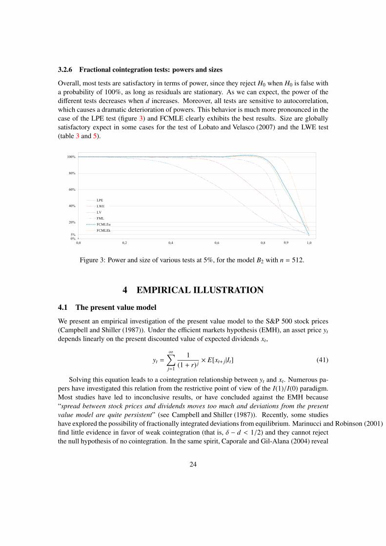
Overall, most tests are satisfactory in terms of power, since they reject H0 when H0 is false witha probability of 100%, as long as residuals are stationary. As we can expect, the power of thedifferent tests decreases when d increases. Moreover, all tests are sensitive to autocorrelation,which causes a dramatic deterioration of powers. This behavior is much more pronounced in thecase of the LPE test (figure 3) and FCMLE clearly exhibits the best results. Size are globallysatisfactory expect in some cases for the test of Lobato and Velasco (2007) and the LWE test(table 3 and 5).

0%

20%

40%

60%

80%

100%

0,0 0,2 0,4 0,6 0,8 1,0

LPE

LWE

LV

FML

FCMLEu

FCMLEk5%

0,9

Figure 3: Power and size of various tests at 5%, for the model B2 with n = 512.

4 EMPIRICAL ILLUSTRATION

4.1 The present value model

We present an empirical investigation of the present value model to the S&P 500 stock prices(Campbell and Shiller (1987)). Under the efficient markets hypothesis (EMH), an asset price yt

depends linearly on the present discounted value of expected dividends xt,

yt =

∞∑j=1

1(1 + r) j × E[xt+ j|It] (41)

Solving this equation leads to a cointegration relationship between yt and xt. Numerous pa-pers have investigated this relation from the restrictive point of view of the I(1)/I(0) paradigm.Most studies have led to inconclusive results, or have concluded against the EMH because“spread between stock prices and dividends moves too much and deviations from the presentvalue model are quite persistent” (see Campbell and Shiller (1987)). Recently, some studieshave explored the possibility of fractionally integrated deviations from equilibrium. Marinucci and Robinson (2001)find little evidence in favor of weak cointegration (that is, δ − d < 1/2) and they cannot rejectthe null hypothesis of no cointegration. In the same spirit, Caporale and Gil-Alana (2004) reveal

24

strong evidence of in favor weak fractional cointegration with d ∈ [0.6, 0.7] and conclude to therejection of the null hypothesis.

4.2 Estimations results

In order to test the EMH, we use the updated monthly database of Campbell and Shiller (1987)5:yt refers to the Standard and Poor’s composite stock price index from January 1871 to December2011 and xt refers to the associated dividends.

Firstly, we lead several integration tests upon yt and xt including the fractional Wald testof Lobato and Velasco (2007). Results support the hypothesis of non-stationary I(1) processfor both yt and xt. The LV test confirms that processes are both I(1), against the alternativehypothesis of I(d) processes.

Table 7: Unit root testsS&P500 Dividend

Sample (T ) 1871-2010 (1667) 1871-2010 (1667)

(µ) KPSS ADF PP LV KPSS ADF PP LV

Level 30.14 1.085 0.730 0.898 31.64 3.964 1.709 0.16

Difference 0.266 -30.32 -29.98 - 0.674 -9.903 -9.709 -

Crit. value at 5% 0.463 -2.864 -2.864 -1.96 0.463 -2.864 -2.864 -1.96

(µ + δt) KPSS ADF PP LV KPSS ADF PP LV

Level 6.559 -1.639 -1.878 - 6.340 -2.153 -1.900 -

Difference 5.789 -74.28 -62.88 - 4.084 -152.6 -88.16 -

Crit. value at 5% 0.146 -3.415 -3.415 - 0.146 -3.415 -3.415 -

Secondly, we lead several estimations corresponding to different sample sizes. We considerfirst the original dataset of Campbell and Shiller (1987). Next, we consider the complete sample.Finally we consider the complete sample excluding the Cowles (1939)’s data (i.e. from 1871to 1926), since calculation methods are different. We perform estimations using the FCMLEand we also report the Cheung and Lai (1993) methodology and the combination LSE,FML.Results are reported in the table (8).

Results depend heavily on the period and the estimation method. For instance, the method-ology of Cheung and Lai (1993) cannot reject at 5% the null hypothesis of no cointegration(TLPE = −1.43 > −2.25) as well as our one step methodology, when we consider the completesample. Conversely, the LSE/FML methodology reject the null hypothesis accepting cointe-gration (TFML = −3.79 < −1.645). Removing the Cowles (1939)’s data, the conclusion is thesame for the LSE/LPE methodology (TLPE = −1.07 > −2.25), whereas the LSE/FML andthe FCMLE both lead to reject the null hypothesis (TFML = −2.87 < −1.645 and WFCMLE =

−2.40 < −1.645). According to the data set used by Campbell and Shiller (1987), the LSE/LPEand the LSE/FML reject H0 (TFML = −4.21 < −1.645 and TLPE = −3.28 < −1.645) while

5http://www.econ.yale.edu/ shiller/

25

Table 8: Estimation of β, d and tests(n) 1871-2011 (1680) 1926-2011 (1032) 1871-1986 (1380)

θ FCMLE LSE/LPE LSE/FML FCMLE LSE/LPE LSE/FML FCMLE LSE/LPE LSE/FML

d 1.0061 0.7959 0.9086 0.8611 0.8812 0.8510 0.9984 0.6549 0.7913

(0.0318) (0.1158) (0.0424) (0,10172) (0.1346) (0.0517) (0.0329) (0.1232) (0.0495)

β 0.8973 1.1819 1.1819 1.0298 1.2572 1.2572 0.8588 1.0638 1.0638

(0.1379) (0.0046) (0.0046) (0.1967) (0.0073) (0.0073) (0.1416) (0.0058) (0.0058)

α111 0.2531 - 0.3618 0.3786 - 0.3899 0.2575 - 0.4309

(0.0512) - (0.0479) (0.1214) - (0.0586) (0.0557) - (0.0543)

α211 -0.0567 - -0.1056 - - - -0.0498 - -

(0.0316) - (0.0257) - - - (0.0336) - -

R2

0.3874 0.9750 0.9750 0.3139 0.9661 0.9661 0.3837 0.9605 0.9605

the FCMLE Wald test cannot reject H0. However, with respect to power of tests, we cannoteliminate any doubt of type I error and results have to be interpreted carefully.

5 FINAL COMMENTSIn this paper we have compared through Monte Carlo simulations the finite sample proper-

ties of different estimation methods of a fractional cointegration model for a wide range of theintegration order of residuals, in the case where the integration order of regressors is known andequal to 1. To improve efficiency, we have proposed to estimate jointly all parameters of interest,using the Gaussian maximum likelihood estimator. Our approach complements the contribu-tions of Hualde and Robinson (2007), which is restricted to weak fractional cointegration (thatis, δ−d < 1/2), and Nielsen (2007) solely concerned with the stationary fractional cointegrationcase (that is, 0 ≤ d < δ < 1/2). We have studied the finite sample properties of the Gaus-sian maximum likelihood estimator and several estimators that operate in two steps. The MonteCarlo experiment shows that our one-step parametric time domain approach compares favorablywith other estimators of β and d and sometimes performs better, even when cointegrating errorsface endogeneity and serial correlation. We have also suggested to use the fractional integrationWald test of Tanaka (1999), which has good power and size according to our simulation. Finally,we have revisited the test of the present value model of Campbell and Shiller (1987) and foundlittle evidence in favor of fractional cointegration.

References[Andrews and Guggenberger (2003)] Andrews, D. W. K., Guggenberger, P. (2003), “A bias-reduced log-

periodogram regression estimator for the long memory parameter,” Econometrica, 71, 675-712

[Baillie and Bollerslev (1994)] Baillie, R. T., Bollerslev, T. (1994), “Cointegration, fractional cointegra-tion and exchange rate dynamics,” Journal of Finance, 49, 737-45.

26

[Campbell and Shiller (1987)] Campbell, J. Y., Shiller, R. J. (1987), “Cointegration and tests of presentvalue models,” Journal of Political Economy, 95, 1062-1088.

[Caporale and Gil-Alana (2002)] Caporale, G. M., Gil-Alana, L. A. (2002), “Unemployment and inputprices: a fractional cointegration approach,” Applied Economics Letters, 9, 347-351.

[Caporale and Gil-Alana (2004)] Caporale, G. M., Gil-Alana, L. A. (2004), “Fractional cointegrationand tests of present value models,” Review of Financial Economics, 13, 245-58.

[Cheung and Lai (1993)] Cheung, Y. W., Lai K. S. (1993), “A fractional cointegration analysis of pur-chasing power parity,” Journal of Business & Economic Statistics, 11, 103-112.

[Cowles (1939)] Cowles, A. (1939), “Common stock indexes,” Bloomington: Principia Press, (2nd ed.).

[da Silva and Robinson (2008)] da Silva, A. G., Robinson, P. M. (2008), “Finite Sample Performancein Cointegration Analysis of Nonlinear Time Series with Long Memory,” Econometric Theory, 27,268-297.

[Dittman (2000)] Dittman, I. (2000), “Residual-based tests for fractional cointegration: a Monte Carlostudy,” Journal Time Series Analysis, 21, 615-47.

[Dolado et al. (2002)] Dolado, J. J., Gonzalo, J., Mayoral, L. (2002), “A Fractional DickeyFuller Test forUnit Roots,” Econometrica, 70, 1963-2006.

[Dubois et al. (2004)] Dubois, E., Lardic, S., Mignon, V. (2004), “The Exact Maximum Likelihood-Based Test for Fractional Cointegration: Critical Values, Power and Size,” Computational Eco-nomics, 24, 239-255.

[Engle and Granger (1987)] Engle, R. F., Granger, C. W. J. (1987), “Cointegration and error correction:representation, estimation and testing,” Econometrica, 55, 251-276.

[Fox and Taqqu (1986)] Fox, R., Taqqu, M. S. (1986), “Large-sample properties of parameter estimatesfor strongly dependent stationary gaussian series,” Annals of Statistics 14, 517-532.

[Geweke and Porter-Hudak (1983)] Geweke, J., Porter-Hudak, S. (1983), “The estimation and applica-tion of long memory time series models,” Journal of Time Series Analysis 4, 221-238.

[Granger (1986)] Granger, C. W. J. (1986), “Developments in the Study of Cointegrated Economic Vari-ables,” Oxford Bulletin of Economics and Statistics, 48, 213-228.

[Granger and Joyeux (1980)] Granger, C. W. J., Joyeux, R. (1980), “An introduction to long memorytime series models and fractional differencing,” Journal of Time Series Analysis, 1, 15-29.

[Henry and Zaffaroni (2003)] Henry, M., Zaffaroni, P. (2003), “The long range dependence paradigmfor macroeconomics and finance,” In: Doukhan, P., Oppenheim, G., Taqqu, M. S., eds. Theory andApplications of Long-Range Dependence. Boston: Birkhuser, pp. 417-438.

[Hidalgo and Robinson (2002)] Hidalgo, F. J., Robinson, P. M. (2002), “Adapting to Unknown Distur-bance Autocorrelation in Regression With Long Memory,” Econometrica, 70, 1545-1581.

[Hosking (1981)] Hosking, J.R.M. (1981), “Fractional differencing,” Biometrika 68, 165-176.

[Hualde and Robinson (2007)] Hualde, J., Robinson, P. M. (2007), “Root-n-consistent estimation ofweak fractional cointegration,” Journal of Econometrics, 140, 450-484.

27

[Johansen (1988)] Johansen, S. (1988). “Statistical analysis of cointegrating vectors,” Journal of Eco-nomic Dynamics and Control, 12, 231-54.

[Kunsch (1987)] Kunsch, H. R. (1987), “Statistical aspects of self-similar processes,” In: Prokhorov, Y.,Sazanov, V. V., eds. Proceedings of the First World Congress of the Bernoulli Society. Utrecht: VNUScience Press, pp. 67-74.

[Kurozumi and Hayakawa (2009)] Kurozumi, E., Hayakawa, K. (2009), “Asymptotic properties of theefficient estimators for cointegrating regression models with serially dependent errors,” Journal ofEconometrics, 149, 118-135.

[Lasak (2010)] Lasak, K. (2010), “Maximum likelihood estimation of fractionally cointegrated systems,”CREATES Research Paper, 2008-53.

[Lobato and Velasco (2007)] Lobato, I. N., Velasco, C. (2007), “Efficient Wald tests for fractional unitroots,” Econometrica, 75, 575-589.

[Marinucci and Robinson (2001)] Marinucci, D., Robinson, P. M. (2001), “Semiparametric fractionalcointegration,” Journal of Econometrics, 105, 225-47.

[Nielsen (2004)] Nielsen, M. Ø. (2004), “Optimal Residual-Based Tests for Fractional Cointegration andExchange Rate Dynamics,” Journal of Business & Economic Statistics, 22, 331-345.

[Nielsen (2007)] Nielsen, M. Ø. (2007), “Local Whittle Analysis of Stationary Fractional Cointegrationand the Implied-Realized Volatility Relation,” Journal of Business & Economic Statistics, 25, 427-446.

[Nielsen and Frederiksen (2005)] Nielsen, M. Ø., Frederiksen, P. H. (2005), “Finite Sample Comparisonof Parametric, Semi-parametric, And Wavelet Estimators of Fractional Integration,” EconometricReviews, 24, 405-443.

[Nielsen and Frederiksen (2011)] Nielsen, M. Ø., Frederiksen, P. H. (2011), “Fully modified narrow-band least squares estimation of weak fractional cointegration,” Econometrics Journal, 14, 77-120.

[Panopoulou and Pittis (2004)] Panopoulou, E., Pittis, N. (2004), “A comparison of autoregressive dis-tributed lag and dynamic LSE cointegration estimators in the case of a serially correlated cointegra-tion error,” Econometrics Journal, 7, 585-617.

[Phillips and Hansen (1990)] Phillips, P. C. B., Hansen, B. E. (1990), “Statistical inference in instrumen-tal regressions with I(1) processes,” Review of Economic Studies, 57, 99-125.

[Prais and Winsten (1954)] Prais, S. J., Winsten, C. B. (1954), “Trend Estimators and Serial Correlation,”Cowles Commission Discussion Paper, 383, Chicago.

[Robinson (1991)] Robinson, P. M. (1991), “Testing for Strong Serial Correlation and Dynamic Condi-tional Heteroskedasticity in Multiple Regression,” Journal of Econometrics, 47, 67-84.

[Robinson (1994)] Robinson, P. M. (1994), “Semiparametric analysis of long-memory time series,” An-nals of Statistics, 22, 515-539.

[Robinson (1995)] Robinson, P. M. (1995), “Gaussian semiparametric estimation of long range depen-dence,” Annals of Statistics, 23, 1630-1661.

28

[Robinson and Hidalgo (1997)] Robinson, P. M., Hidalgo, F. J. (1997), “Time series regression withlong-range dependence,” The Annals of Statistics, 25, 77-104.

[Robinson and Hualde (2003)] Robinson, P.M., Hualde, J. (2003), “Cointegration in fractional systemswith unkown integration orders,” Econometrica, 71, 1727-1766

[Robinson and Marinucci (2001)] Robinson, P. M., Marinucci, D. (2001), “Narrow-Band Analysis ofNonstationary Processes,” The Annals of Statistics, 29, 947-986.

[Saikkonen (1995)] Saikkonen, P. (1995), “Problems with the Asymptotic Theory of Maximum Likeli-hood in Integrated and Cointegrated Systems,” Econometric Theory, 11, 888-911.

[Schwarz (1978)] Schwarz, G. E. (1978), “Estimating the dimension of a model,” Annals of Statistics, 6,461-464.

[Sephton (2002)] Sephton, P. S. (2002), “Fractional cointegration: Monte Carlo estimates of criticalvalues, with an application,” Applied Financial Economics, 12, 331-335.

[Stock (1987)] Stock, J. H. (1987), “Asymptotic properties of least squares estimators of cointegratingvector,” Econometrica, 55, 1035-1056.

[Stock and Watson (1993)] Stock, J. H., Watson, M.W. (1993), “A simple estimator of cointegrating vec-tors in higher-order integrated systems,” Econometrica, 61, 783-820.

[Sowell (1992)] Sowell, F. B. (1992), “Maximum likelihood estimation of stationary univariate fraction-ally integrated time series models,” Journal of Econometrics, 53, 165-188.

[Tanaka (1999)] Tanaka, K. (1999), “The nonstationary fractional unit root,” Econometric Theory, 15,549-582.

29