Parameter estimation for the discretely observedfractional Ornstein-Uhlenbeck process and the

Yuima R package

Alexandre Brouste∗

Laboratoire Manceau de MathematiquesUniversite du Maine

Avenue Olivier Messiaen - 72100 Le Mans, France

Stefano M. Iacus†

Department of Economics, Business and StatisticsUniversity of Milan

Via Conservatorio, 7 - 20122 Milan, Italy

Abstract

This paper proposes consistent and asymptotically Gaussian estimatorsfor the parameters λ, σ and H of the discretely observed fractional Ornstein-Uhlenbeck process solution of the stochastic differential equation dYt =−λYtdt + σdWH

t , where (WHt , t ≥ 0) is the fractional Brownian motion.

For the estimation of the drift λ, the results are obtained only in the casewhen 1

2 < H < 34 . This paper also provides ready-to-use software for the R

statistical environment based on the YUIMA package.

1 Introduction

Statistical inference for parameters of ergodic diffusion processes observed on dis-crete increasing grid have been much studied. Local asymptotic normality (LAN)property of the likelihoods have been shown in [10] for elliptic ergodic diffusion,

∗E-mail: alexandre.brouste@univ-lemans.fr, corresponding author.†E-mail: stefano.iacus@unimi.it

1

arX

iv:1

112.

3777

v1 [

stat

.CO

] 1

6 D

ec 2

011

under proper conditions for the drift and the diffusion coefficient, and a meshsatisfying

∆N −→ 0 and N∆N −→ +∞when the size of the sample N grows to infinity. Estimation procedure have beenstudied by many authors, mainly in the one-dimensional case (see, for instance,[8, 14] and [26] in the multidimensional setting). All estimators in the previousworks are based on contrasts (for contrasts framework, see [9]), assuming in thegeneral case, that for some p > 1, as n −→ +∞, N∆p

N −→ 0. In particular,for Ornstein-Uhlenbeck process, transitions densities are known, and all have beentreated, as remarked in [13].

In the fractional case, we consider the fraction Ornstein-Uhlenbeck process(fOU), the solution of

dYt = −λYtdt+ σdWHt

where WH =(WHt , t ≥ 0

)is a normalized fractional Brownian motion (fBM), i.e.

the zero mean Gaussian processes with covariance function

EWHs W

Ht =

1

2

(|s|2H + |t|2H − |t− s|2H

)with Hurst exponent H ∈ (0, 1). The fOU process is neither Markovian nor asemimartingale for H 6= 1

2but remains Gaussian and ergodic (see [5]). For H >

12, it even presents the long-range dependance property that makes it useful for

different applications in biology, physics, ethernet traffic or finance.Statistical large sample properties of Maximum Likelihood Estimator of the

drift parameter in the continuous observations case have been treated in [1, 4, 6, 15]for different applications. Moreover, asymptotical properties of the Least SquaresEstimator have been studied in [11].

In the discrete case and fractional case, we can cite few works on the topic. Onthe one hand, very recent works give methods to estimate the drift λ by contrastprocedure [17, 20] or the drift λ and the diffusion coefficient σ with discretizationprocedure of integral transform [25]. In these papers, the Hurst exponent is sup-posed to be known and only consistency is obtained. On the other hand, methodsto estimate the Hurst exponent H and the diffusion coefficient are presented in [3]with classical order 2 variations convolution filters.

To the best of our knowledge, nothing have been done, to have a completeestimation procedure that could estimate all Hurst exponent, diffusion coefficientand drift parameter with central limit theorems and this is the gap we fill in thispaper. Moreover, estimates of H, σ and λ presented in this paper slightly differfrom all those studied previously.

In Section 2 we review the basic facts of stochastic differential equations drivenby the fractional Brownian motion and we introduce the basic notations and as-sumptions. Section 3 presents consistent and asymptotically Gaussian estimators

2

of the parameters of the fractional Ornstein-Uhlenbeck process from discrete ob-servations. In Section 4 we present ready-to-use software for the R statisticalenvironment which allows the user to simulate and estimate the parameters of thefOU process. We further present Monte-Carlo experiments to test the performanceof the estimators under different sampling conditions.

2 Model specification

Let X = (Yt, t ≥ 0) be a fractional Ornstein-Uhlenbeck process (fOU), i.e. thesolution of

Yt = y0 − λ∫ t

0

Ysds+ σWHt , t > 0, Y0 = y0, (1)

where unknown parameter ϑ = (λ, σ,H) belongs to an open subset Θ of (0,Λ) ×[σ, σ] × (0, 1), 0 < Λ < +∞, 0 < σ < σ < +∞ and WH = (WH

t , t ≥ 0) is astandard fractional Brownian motion [16, 18] of Hurst parameter H ∈ (0, 1), i.e.a Gaussian centered process of covariance function

EWHt W

Hs =

1

2

(t2H + s2H − |t− s|2H

).

It is worth emphasizing that in the case H = 12, W

12 is the classical Wiener

process The fOU process is neither Markovian nor a semimartingale for H 6= 12

but remains Gaussian and ergodic. For H > 12, it even presents the long-range

dependance property (see [5]).The present work exposes an estimation procedure for estimating all three

components of ϑ given the regular discretization of the sample path Y T = (Yt, 0 ≤t ≤ T ), precisely

(Xn := Yn∆N, n = 0 . . . N) ,

where T = TN = N∆N −→ +∞ and ∆N −→ 0 as N −→ +∞.

In the following, convergencesL−→,

p−→ anda.s.−→ stand respectively for the con-

vergence in law, the convergence in probability and the almost-sure convergence.

3 Estimation procedure

Contrary to the previous works on the subject, we consider here the problemof estimation of H, σ and λ when all parameters are unknown, using discreteobservations from the fractional Ornstein-Uhlenbeck process. Due to the fact thatone can estimate H and σ without the knowledge of λ, our approach consistsnaturally in a two step procedure.

3

3.1 Estimation of the Hurst exponent H and the diffusioncoefficient σ with quadratic generalized variations

The key point of this paper is that the Hurst exponent H and the diffusion coef-ficient σ can be estimated without estimating λ.

Let a = (a0, . . . , aK) be a discrete filter of length K + 1, K ∈ N, and of orderL ≥ 1, K ≥ L, i.e.

K∑k=0

akk` = 0 for 0 ≤ ` ≤ L− 1 and

K∑k=0

akkL 6= 0. (2)

Let it be normalized withK∑k=0

(−1)1−kak = 1 . (3)

In the following, we will also consider dilatated filter a2 associated to a defined by

a2k =

{ak′ if k = 2k′

0 sinon.for 0 ≤ k ≤ 2K .

Since2K∑k=0

a2kk

r = 2rK∑k=0

krak, filter a2 as the same order than a. We denote by

VN,a =N−K∑i=0

(K∑k=0

akXi+k

)2

the generalized quadratic variations associated to the filter a (see for instance [12])and, finally,

HN =1

2log2

VN,a2

VN,a

and

σN =

2 · − VN,a∑k,` aka`|k − `|2HN ∆2HN

N

12

.

Theorem 1. Let a be a filter of order L ≥ 2. Then, both estimators HN and σNare strongly consistent, i.e.

(HN , σN)a.s.−→ (H, σ) as N −→ +∞.

4

Moreover, we have asymptotical normality property, i.e. as N → +∞, for allH ∈ (0, 1), √

N(HN −H)L−→ N (0,Γ1(ϑ, a))

and √N

logN(σN − σ)

L−→ N (0,Γ2(ϑ, a))

where Γ1(ϑ, a) and Γ2(ϑ, a) symmetric definite positive matrices depending on σ,H, λ and the filter a.

Proof. The solution of (1) can be explicited

Yt = x0e−λt + σ

∫ t

0

e−λ(t−s)dWHs ,

where the integral is defined as a Riemann-Stieljes pathwise integral. Let us con-sider the stationary centered Gaussian solution

Y †t = σ

∫ t

−∞e−λ(t−u)dWH

u .

We have also,

Y †t − Yt = e−λt(Y †0 − y0

)a.s.−→ 0.

It is known (see [5, Lemma 2.1]) that

EY †0 (Y †0 − Y†t ) = −σ2H(2H − 1)e−λt

∫ 0

−∞eλu(∫ t

0

eλv(v − u)2H−2dv

)du.

Let v(t) denote the variogram of Y †t . We now show that

v(t) = E(Y †0

)2

− EY †t Y†

0 =σ2

2|t|2H + r(t)

5

where r(t) = o(|t|2H) as t tends to zero. Indeed,

v(t) = −σ2H(2H − 1)

∫ 0

−∞eλu(∫ t

0

e−λ(t−v)(v − u)2H−2dv

)du

= −σ2H(2H − 1)

∫ 0

−∞eλu(∫ t

0

e−λr(t− r − u)2H−2dr

)du

= −σ2H(2H − 1)

∫ ∞0

∫ t

0

e−λ(r+u)(t− r + u)2H−2drdu

= −σ2H(2H − 1)

∫ ∞0

∫ u+t

u

e−λw(t− w + 2u)2H−2dwdu

= −σ2H(2H − 1)

∫ ∞0

e−λw(∫ w

max(0,w−t)(t− w + 2u)2H−2du

)dw

= −1

2σ2H(2H − 1)

∫ ∞0

e−λw(∫ t+w

|t−w|x2H−2dx

)dw.

Thus,

dv

dt(t) = −1

2σ2H(2H − 1)

∫ ∞0

e−λw((t+ w)2H−2 − |t− w|2H−2

)dw

= −1

2σ2H(2H − 1)t2H−1

∫ ∞0

e−λty((1 + y)2H−2 − |1− y|2H−2

)dy

= −1

2σ2H(2H − 1)t2H−1

∫ ∞0

((1 + y)2H−2 − |1− y|2H−2

)dy︸ ︷︷ ︸

<∞

+r(t)

= σ2Ht2H−1 + r(t)

with

r(t) = −1

2σ2H(2H − 1)t2H−1

∞∑i=1

∫ ∞0

(−λty)i

i!

((1 + y)2H−2 − |1− y|2H−2

)dy.

Therefore, we proved that

v(t) =σ2

2|t|2H + r(t).

Now, applying results in [12, Theorem 3(i)], the proof of Theorem 1 is completebecause the following conditions are fulfilled:

• firstly, r(t) = o(|t|2H) as t tends to zero,

6

• secondly, for classical generalized quadratic variations or order L ≥ 2 (forinstance L = 2),

|r(4)(t)| ≤ G|t|2H+1−ε−4

with 2H+1−ε > 2H and 4 > 2H+1−ε+1/2 for ε < 1 and any H ∈ (1/2, 1).

Remark 1. We have two useful examples of filters. Classical filters of order L ≥ 1are defined by

ak = cL,k =(−1)1−k

2K

(Kk

)=

(−1)1−k

2KK!

k!(K − k)!pour 0 ≤ k ≤ K.

Daubechies filters of even order can also be considered (see [7]), for instancethe order 2 Daubechies’ filter:

1√2

(.4829629131445341,−.8365163037378077, .2241438680420134, .1294095225512603).

Remark 2. For classical order 1 quadratic variations (L = 1) and a =(−1

2, 1

2

)we can also obtain consistency for any value of H, but the central limit theoremholds only for H < 3

4(see [12]).

3.2 Estimation of the drift parameter λ when both H andσ are unknown

From [11], we know the following result

limt−→∞

var(Yt) = limt−→∞

1

t

∫ t

0

Y 2t dt =

σ2Γ (2H + 1)

2λ2H=: µ2 .

This gives a natural plug-in estimator of λ, namely

λN =

2 µ2,N

σ2NΓ(

2HN + 1)− 1

2HN

where µ2,N is the empirical moment of order 2, i.e

µ2,N =1

N

N∑n=1

X2n.

7

Theorem 2. Let H ∈(

12, 3

4

)and a mesh satisfying the condition N∆p

N −→ 0,p > 1, as N −→ +∞. Then, as N −→ +∞,

λNa.s.−→ λ

and √TN

(λN − λ

)L−→ N (0,Γ3(ϑ)),

where Γ3(ϑ) = λ(σH2H

)2and

σ2H = (4H − 1)

(1 +

Γ(1− 4H)Γ(4H − 1)

Γ(2− 2H)Γ(2H)

). (4)

Proof. Let us note TN = N∆N . It had been shown in [11] that, as TN → +∞ (oras N → +∞),

1

TN

∫ TN

0

X2t dt

a.s.−→ κHλ−2H (5)

and, with straightforward calculus,√TN

(1

TN

∫ TN

0

X2t dt− κHλ−2H

)L−→ N (0, (σHκH)2 λ−4H−1) (6)

where κH = σ2 Γ(2H+1)2

and σH is defined by (4). Let us denote µ2,N the discretiza-tion of the integral

µ2,N =1

N

N∑n=1

X2n and µ2 = κHλ

−2H .

Then√TN (µ2,N − µ2) =

√TN

(µ2,N −

1

TN

∫ TN

0

X2t dt

)+√TN

(1

TN

∫ TN

0

X2t dt− µ2

).

As (Xt, t ≥ 0) is a Gaussian process and Holder of order 12< H < 3

4, we have

√TN

(µ2,N − 1

TN

∫ TN0

X2t dt)

p−→ 0 as N −→ +∞ provided that N∆pN −→ 0,

p > 1, (see [14, Lemma 8]), we deduce from (5) and (6) that√TN (µ2,N − µ2)

L−→ N(0, (σHκH)2 λ−4H−1

). (7)

Let us introduce the following two quanitites

MN =

µ2,N

HN

σN

and m =

µ2

Hσ

.

8

Finally, results obtained in Theorem 1 and the convergence in (7) gives consistency

of MN , i.e. MNP−→ m as as N −→ +∞. Let us further define

g(µ2, H, σ) =

(2µ2

σ2Γ(2H + 1)

)− 12H

.

The derivatives of g with respect to σ, H and µ2 are bounded when 0 < Λ < +∞,0 < σ < σ < +∞ and 1

2< H < 3

4. Therefore, as ∆N (logN)2 −→ 0 as N −→ +∞,

we can obtain by Taylor expansion that√TN (g(MN)− g(m))

L−→ N (0, g′µ2(m)2 (σHκH)2 λ−4H−1)

or √TN

(λN − λ

)L−→ N (0,Γ3(ϑ))

where Γ3(ϑ) = g′µ2(m)2 (σHκH)2 λ−4H−1 = λ(σH2H

)2, g′µ2(.) is the derivative of g

with respect to µ2 andλN

a.s.−→ λ

as N −→ +∞.

Remark 3. The different conditions on ∆N raise the question of whether such arate actually exists. One possible mesh is ∆N = logN

N.

Remark 4. As in the classical case H = 12, the limit variance Γ3(ϑ) does not

depend on the diffusion coefficient σ. Let us also notice that the quantity σ2H

appearing in Γ3(ϑ) is an increasing function of H.

4 Statistical software and Monte-Carlo analysis

In this section we present a brief introduction to the yuima package for R statisticalenvironment [21]. The yuima package is a comprehensive framework, based on theS4 system of classes and methods, which allows for the description of solutions ofstochastic differential equations. Although we cannot give details here, the usercan specify a stochastic differential equation of the form

dXt = b(t,Xt)dt+ σ(t,Xt)dWHt + c(t,Xt)Zt

where the coefficients b(·, ·), σ(·, ·) and c(·, ·) are entirely specified by the user,even in parametric form; (Zt, t ≥ 0) is a Levy process (for more information onLevy processes, see [2, 22] and (WH

t , t ≥ 0) is a fractional Brownian motion (recall

9

that (W12t , t ≥ 0) is the standard Brownian motion). The Levy process (Zt, t ≥ 0)

and the fractional Brownian motion (WHt , t ≥ 0) can be present at the same time

only when H = 12, but all other combinations are possible. The yuima package

provides the user, not only the simulation part, but also several parametric andnon-parametric estimation procedures. In the next section we present an exampleof use only for simulation and estimation of the fractional Ornstein-Uhlenbeckprocess considered in this paper.

To test the performance of the estimators for finite samples, we run a Monte-Carlo analysis. We consider different setup for the parameters even outside theregion 1

2< H < 3

4and different sample size with large and small values of T in

order to test the performance of the estimator of the drift parameter when thestationarity is not reached by the process. All numerical experiments presented inthe following have been done with the yuima package [23].

4.1 Example of numerical simulation and estimation of thefOU process with the yuima package

With the yuima package the fractional Gaussian noise is simulated with the Woodand Chan method [24] or other techniques. We present below how to simulate onesample path of the fractional Ornstein-Uhlenbeck process with Euler-Maruyamamethod. For instance, loading the package with

library(yuima)

we can simulate a regularly sampled path of the following model

Xt = 1− 2

∫ t

0

Xtdt+ dWHt , H = 0.7,

with

samp <-setSampling(Terminal=100, n=10000)

mod <- setModel(drift="-2*x", diffusion="1",hurst=0.7)

ou <- setYuima(model=mod, sampling=samp)

fou <- simulate(ou, xinit=1)

The estimation procedure of the Hurst parameter have been implemented in qgv

function. In order to estimate only the parameter H, one can use

qgv(fou)

that works also for non linear fractional diffusions (see [19]). The procedure forjoint estimation of the Hurst exponent H, diffusion coefficient σ and drift param-eter λ is called lse(,frac=TRUE). So for example, in order to estimate the threedifferent parameters H, λ and σ, one can use

10

lse(fou,frac=TRUE)

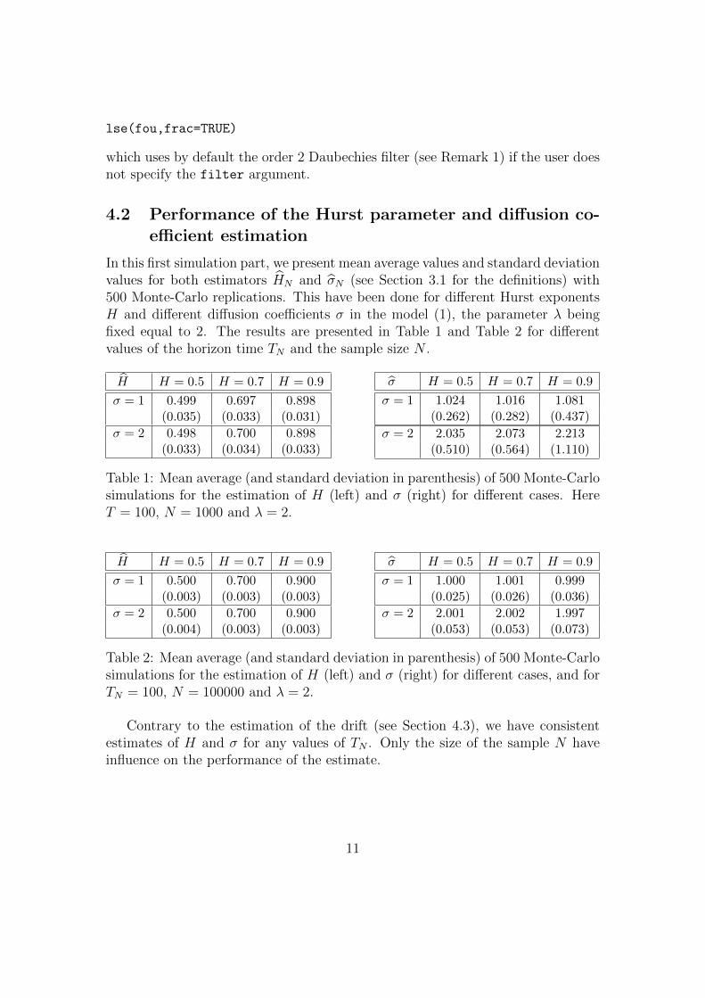
which uses by default the order 2 Daubechies filter (see Remark 1) if the user doesnot specify the filter argument.

4.2 Performance of the Hurst parameter and diffusion co-efficient estimation

In this first simulation part, we present mean average values and standard deviationvalues for both estimators HN and σN (see Section 3.1 for the definitions) with500 Monte-Carlo replications. This have been done for different Hurst exponentsH and different diffusion coefficients σ in the model (1), the parameter λ beingfixed equal to 2. The results are presented in Table 1 and Table 2 for differentvalues of the horizon time TN and the sample size N .

H H = 0.5 H = 0.7 H = 0.9

σ = 1 0.499 0.697 0.898(0.035) (0.033) (0.031)

σ = 2 0.498 0.700 0.898(0.033) (0.034) (0.033)

σ H = 0.5 H = 0.7 H = 0.9

σ = 1 1.024 1.016 1.081(0.262) (0.282) (0.437)

σ = 2 2.035 2.073 2.213(0.510) (0.564) (1.110)

Table 1: Mean average (and standard deviation in parenthesis) of 500 Monte-Carlosimulations for the estimation of H (left) and σ (right) for different cases. HereT = 100, N = 1000 and λ = 2.

H H = 0.5 H = 0.7 H = 0.9

σ = 1 0.500 0.700 0.900(0.003) (0.003) (0.003)

σ = 2 0.500 0.700 0.900(0.004) (0.003) (0.003)

σ H = 0.5 H = 0.7 H = 0.9

σ = 1 1.000 1.001 0.999(0.025) (0.026) (0.036)

σ = 2 2.001 2.002 1.997(0.053) (0.053) (0.073)

Table 2: Mean average (and standard deviation in parenthesis) of 500 Monte-Carlosimulations for the estimation of H (left) and σ (right) for different cases, and forTN = 100, N = 100000 and λ = 2.

Contrary to the estimation of the drift (see Section 4.3), we have consistentestimates of H and σ for any values of TN . Only the size of the sample N haveinfluence on the performance of the estimate.

11

4.3 Plug-in for the estimation of drift parameter λ

In this second simulation part, we present mean average values and standard de-viation values for the estimator λN (see Section 3.2 for the definition) of the driftwith 500 Monte-Carlo replications. This have been done for different values of λand H in model (1), the diffusion coefficient σ being fixed to 1 (see Remark 4).The results are presented in Table 3 for different values of the horizon time TNand the sample size N .

H = 0.5 H = 0.6 H = 0.7

λ = 0.5 0.093 0.214 0.353(0.037) (0.057) (0.069)

λ = 1 0.138 0.276 0.432(0.052) (0.068) (0.078)

H = 0.5 H = 0.6 H = 0.7

λ = 0.5 0.476 0.514 0.605(0.148) (0.166) (0.298)

λ = 1 0.906 0.940 1.005(0.227) (0.238) (0.412)

Table 3: Mean average (and standard deviation in parenthesis) of 500 Monte-Carlosimulation for the estimation of λ for different values of H and λ. Here σ = 1 andTN = 1 and N = 100000 (left) and TN = 100 and N = 1000 (right).

We can see in Table 3 that the values of TN is important for the estimation ofthe drift. Actually, the consistency of the estimates are valid for increasing valuesof TN and decreasing values of the mesh size ∆N . Moreover, the bigger H, theharder the estimation of the drift parameter. This phenomena can be explainedby the long-range dependence property of the fOU process. It is the same for λ ;as λ increases, its estimation is harder (see Remark 4). It can be explained by thefact that when λ is bigger, the fOU process enters faster in its stationary behaviorwhere it is more difficult to detect the trend.

Finally, in order to illustrate the asymptotical normality for the estimator λ ofλ, we present in Figure 1 the kernel estimation of the density.

Acknowledgments

We would like to thank Marina Kleptsyna for the discussions and her interestfor this work. Computing resources have been financed by Mostapad project inCNRS FR 2962. This work has been supported by the project PRIN 2009JW2STY,Ministero dell’Istruzione dell’Universita e della Ricerca.

References

[1] B. Bercu, L. Coutin, and N. Savy. Sharp large deviations for the fractionalOrnstein-Uhlenbeck process. Teoriya Veroyatnostei i ee Primeneniya, 2010.

12

-4 -2 0 2 4

0.0

0.1

0.2

0.3

Density

EstimatedTheoretical

Figure 1: Kernel estimation for the density of(√

TN

(λ

(m)N − λ

))m=1...M

, M =

5000, for TN = 1000 and TN = 100000 (fill line) and the theoretical Gaussiandensity N (0,Γ3(ϑ)) (dashed line) for ϑ = (λ, σ,H) = (0.3, 1, 0.7) (for the value ofΓ3(ϑ) see Theorem 2).

[2] J. Bertoin. Levy Processes. Cambridge University Press, Cambridge, 1998.

[3] C. Berzin and J. Leon. Estimation in models driven by fractional brownianmotion. Annales de l’Institut Henri Poincare, 44(2):191–213, 2008.

[4] A. Brouste and M. Kleptsyna. Asymptotic properties of MLE for partiallyobserved fractional diffusion system. Statistical Inference for Stochastic Pro-cesses, 13(1):1–13, 2010.

[5] P. Cheridito, H. Kawaguchi, and M. Maejima. Fractional Ornstein-Uhlenbeckprocesses. Electronic Journal of Probability, 8(3):1–14, 2003.

[6] I. Cialenco, S. Lototsky, and J. Pospisil. Asymptotic properties of the max-imum likelihood estimator for stochastic parabolic equations with additivefractional Brownian motion. Stochastics and Dynamics, 9(2):169–185, 2009.

[7] I. Daubechies. Ten Lectures on Wavelets. SIAM, 1992.

[8] D. Florens-Zmirou. Approximate discrete time schemes for statistics of diffu-sion processes. Statistics, 20:263–284, 1989.

[9] V. Genon-Catalot. Maximum constrast estimation for diffusion processes fromdiscrete observation. Statistics, 21:99–116, 1990.

13

[10] E. Gobet. Lan property for ergodic diffusions with discrete observations.Annales de l’Institut Henri Poincare, 38(5):711–737, 2002.

[11] Y. Hu and D. Nualart. Parameter estimation for fractional ornstein-uhlenbeckprocesses. Statistics and Probability Letters, 80(11-12):1030–1038, 2010.

[12] J. Istas and G. Lang. Quadratic variations and estimation of the local hlderindex of a gaussian process. Annales de l’Institut Henri Poincare, 23(4):407–436, 1997.

[13] J. Jacod. Inference for stochastic processes. Statistics, Prepublication 683,2001.

[14] M. Kessler. Estimation of an ergodic diffusion from discrete observations.Scandinavian Journal of Statistics, 24:211–229, 1997.

[15] M. Kleptsyna and A. Le Breton. Statistical analysis of the fractional Ornstein-Uhlenbeck type process. Statistical Inference for Stochastic Processes, 5:229–241, 2002.

[16] A. Kolmogorov. Winersche Spiralen und einige andere interessante Kurven inHilbertschen Raum. Acad. Sci. USSR, 26:115–118, 1940.

[17] C. Ludena. Minimum contrast estimation for fractional diffusion. Scandina-vian Journal of Statistics, 31:613–628, 2004.

[18] B. Mandelbrot and J. Van Ness. Fractional Brownian motions, fractionalnoises and application. SIAM Review, 10:422–437, 1968.

[19] D. Melichov. On estimation of the Hurst index of solutions of stochasticequations. PhD thesis, Vilnius Gediminas Technical University, 2011.

[20] A. Neuenkirch and S. Tindel. A Least Square-type procedure for parameterestimation in stochastic differential equations with additive fractional noise.preprint, 2011.

[21] R Development Core Team. R: A Language and Environment for StatisticalComputing. R Foundation for Statistical Computing, Vienna, Austria, 2010.ISBN 3-900051-07-0.

[22] K. Sato. Levy Processes and Infinitely Divisible Distributions. CambridgeUniversity Press, Cambridge, 1999.

[23] YUIMA Project Team. yuima: The YUIMA Project package (unstable ver-sion), 2011. R package version 0.1.1936.

14

[24] A. Wood and G. Chan. Simulation of stationary Gaussian processes. Journalof computational and graphical statistics, 3(4):409–432, 1994.

[25] W. Xiao, W. Zhang, and W. Xu. Parameter estimation for fractional ornstein-uhlenbeck processes at discrete observation. Applied Mathematical Modelling,35:4196–4207, 2011.

[26] N. Yoshida. Estimation for diffusion processes from discrete observations.Journal of Multivariate Analysis, 41:220–242, 1992.

15