estimating the relationship between the current account ... · estimating the relationship between...

WP-2017-016

Estimating the Relationship between the Current Account, theCapital Account and Investment for India

Ashima Goyal and Vaishnavi Sharma

Indira Gandhi Institute of Development Research, MumbaiSeptember 2017

Estimating the Relationship between the Current Account, theCapital Account and Investment for India

Ashima Goyal and Vaishnavi Sharma

Email(corresponding author): [email protected]

AbstractCausality from the capital account (KA) to the current account (CA) of the balance of payments

indicates disruption from capital flows while the reverse can indicate smooth financing of the CA that

allows investment to exceed domestic savings. A three-variable vector autoregression tests for Granger

causality between the Indian CA, KA, KA components, and gross fixed capital formation (GFCF) over

2000-01Q1 to 2015-16Q3. Since a current account deficit indicates an excess of investment over savings

it is useful to estimate which type of capital flows affect investment. No causality is found to exist in any

direction between the KA and the CA. There is only indirect causality through some components. Of the

capital flow components only FDI affects GFCF. The latter consistently affects the CA. The CA affects

debt portfolio flows and non-resident deposits, suggesting these were used to finance the CA, but they

were not causal for GFCF. Volatile flows therefore did not deteriorate the CA, but they also did not

contribute to GFCF. India's gradual capital account convertibility may have mitigated shocks from the

KA. Long-term sustainability, however, requires FDI to increase compared to other types of flows.

Keywords: Current Account; Capital Account; Balance of Payments; Granger Causality; GrossFixed Capital Formation

JEL Code: F21, F32

1

Estimating the Relationship between the Current Account, the Capital Account and

Investment for India

1. Introduction

The Balance of Payments (BOP) accounts of almost all nations show large deficits or

surpluses in the recent period of financial liberalization. Given the BOP identity, an

imbalance in the current account (CA) is reflected in the capital account (KA) plus a change

in reserves. Causality from the capital account (KA) to the current account (CA) can indicate

disruption from these capital flows while the reverse can indicate smooth financing of the

CA.

The economic literature does not provide a clear picture of the relationship. Nevertheless

some studies suggest that for advanced economies causality runs from the CA to the KA so

that capital flows finance the CA rather than aggravate it, while in developing nations, the

causality is reversed1.

A current account deficit (CAD) allows much needed investment to exceed domestic savings

for an emerging market. Causality from a KA component to the CA can imply that the

component is used to finance a CAD. But it is also necessary to assess whether the financing

is indeed used for investment. Various components of the KA, such as Foreign Direct

Investment (FDI), Foreign Portfolio Investment (FPI) and ‘debt flows’2 can be expected to

have differing impact on the CA and on investment. FDI is a more stable, long-term

component while FPI and debt flows are relatively volatile, easily influenced by global risk

factors3. The Indian post 1991 industrial policy reforms opened opportunities for foreign

investment4 in various sectors. All this has led to growing KA surpluses in recent years.

There have been periods when the CA also widened. This study, therefore, tries to analyze

1 See Yan and Yang (2008, 2012). Studies that find differing directions of causality include Ersoy (2011), Kim

and Kim (2011), and Lau and Fu (2011). 2 These are the sum total of external assistance, external commercial borrowings (ECB), short-term trade credit,

NRI deposits, FPI debt flows, and Rupee debt service. 3 Yan (2007) finds FDI to cause a CAD in case of Philippines and Canada while FPI causes a CAD for Mexico.

4 Recently India outpaced China and the US with FDI inflows of $31 billion in Jan-June 2015. Also, India

jumped 16 notches to 55 among 140 countries in the World Economic Forum’s Global Competitiveness Index

that ranks countries on the basis of parameters such as institutions, macroeconomic environment, education,

market size and infrastructure among others.

2

these broader aspects of the causal relationship between the two accounts for India for the

time period 2000-01Q1 to 2015-16Q3.

Granger causality tests in a three-variable Vector Autoregression (VAR) indicate whether the

prediction of one variable is significantly improved by including lags of other variable. In a

first step, we check for any causality between the CA and the KA in the presence of

investment. Second, we check for causality between the CA and the main components of the

KA, viz. equity flows and debt flows, again controlling for investment. In a third step, the

equity and debt flows are further disaggregated. We take FDI-equity5 and FPI-equity as the

disaggregated components of total equity flows and from debt flows we take the four major

components of the total debt portfolio, namely FPI-debt flows, short-term (ST) credit, non-

residential Indian (NRI) deposits and External Commercial Borrowings (ECBs). So, we

check for a total of nine causalities.

There is no extensive study on the causal relationship of disaggregated components of total

debt flows on investment and the CA. The results have implications for financial and

macroeconomic stability and for policy. A previous multivariate causality study of the CA

and the KA for India (Garg and Prabheesh, 2015) included the real exchange rate. They did

not find any causal relationship between the two accounts, but found FPI flows to affect the

exchange rate and therefore the CA. Although FPI and equity flows are more volatile, a

managed float with active foreign exchange intervention prevented persistent deviations from

equilibrium real exchange rate in India. It is more important, therefore, to check for causality

with investment as a control. We try to fill this gap.

The remainder of this paper is organized as follows: the next section presents a theoretical

background. Section III provides some stylized facts giving an overview of the Indian BOP.

Section IV provides the dataset and the variables employed. Section V presents the

methodology and Section VI the empirical findings. The last section concludes.

2. Theoretical Background

5 This was 74.4 per cent of FDI on average in this period. The other components of FDI are reinvested earnings

(retained earnings of FDI companies) and ‘other direct capital’ (inter-corporate debt transactions between

related entities).

.

3

According to the BOP identity, the CA and the KA of a country (plus change in foreign

exchange reserves)6 have to be balanced ex post, implying that the deficits (or, surpluses) in

the CA will have to largely match the net capital inflows (or, outflows). Various factors,

however, determine the economic relationship between the two accounts.

Conventionally, CA is specified as a sum of net exports (X-M) and net income from abroad

(R):

CA=(X-M) + R

The basic macroeconomic aggregate demand equals supply identity is:

GDP (Y) = Consumption (C) + Investment (I) + Government Spending (G) + {Exports (X)-

Imports (M)}

National income or production of a country, however, is:

GNP (Gross National Product) = Gross Domestic Product (GDP) + Net factor income from

abroad (R)

From these identities we can derive another definition of current account balance as:

CA = Savings (S) –Investment (I)

The difference between GNP and (C+G) is the level of personal and government savings S.

When domestic savings are lower (or higher) than the level of domestic investment, a country

would, in the net, borrow from (or give credit) abroad to finance a deficit (or surplus) in the

CA. For example, during periods of high investment demand, when domestic savings fall

short, capital inflows from the rest of the world are required. These capital flows are a credit

on the KA and will be matched by a deficit on the CA.

The fundamental BOP equation is an identity, which can be achieved through many types of

adjustments. The accounts indirectly affect each other through macro-economic variables. If

6 Recently the KA has been renamed as a KA and a financial account with change in reserves included in the

financial account following the new international convention. Our dataset and analysis uses the old classification

(see https://www.rbi.org.in/SCRIPTS/PublicationsView.aspx?id=17273). The KA variable does not include the

item E Monetary movements which includes change in official reserves.

4

inflows lead to currency appreciation net imports rise worsening the CA. If they are absorbed

as reserves, however, the change in reserves leads to a corresponding change in the supply of

money, raising domestic demand for non-traded goods, domestic prices, and again

appreciating the currency. But the acquisition of reserves can be sterilized by sale of

government securities.

To the extent capital flows raise investment and capacity, prices will need to rise less, and

some expansion in money supply can be absorbed. A CAD equals net imports but also the

excess of investment over savings. As incomes rise savings and imports will also rise,

assuming constant propensities to save and to import. These leakages reducing domestic

demand, are part of the adjustments that equate the CA to the excess of savings over

investment, with causality running from exogenous shocks to demand components such as

investment and exports and then to output and prices.

Both CA and the KA are therefore affected by similar exogenous factors such as domestic

and foreign income, exchange rates and interest rates. But these exogenous factors differently

impact components of the KA. For example, FDI is more stable and is influenced by long-

term domestic fundamentals while FPI is relatively volatile and is determined by short-term

aspects and speculative considerations. From an emerging market perspective, it is important

to know whether the capital inflows to the economy adjust to changes in the CA (by

financing the deficit of the domestic economy or that of foreign economies in case of

surpluses) or rather lead to disturbances in the CA.

3. Some Stylized Facts of the Indian Economy

From independence till early 80’s, India had a rather closed KA. External financing was

mostly official aid on concessional terms. But in the 80’s, widening CAD due to rise in oil

prices, sharp depreciation of the rupee and increase in imports due to selective liberalization

made the existing import substitution strategy unsustainable. Greater external sources of

financing were required. For the time being India resorted to external commercial borrowings

(ECBs), Non-resident Indian (NRI) deposits and short-term (ST) borrowings. But this was

inadequate under continuing BOP stress. Liberalization of trade and investment regimes was

initiated in 1991 to integrate the Indian economy with that of the world. The reforms have

been gradual and continuous, more like a process than an event. Quantitative restrictions on

imports were phased out with bulk of the tariff lines bound under WTO. Full convertibility of

5

the rupee in the CA prevails. Barring a few industries, FDI with up to 100 per cent ownership

is allowed in most sectors. Foreign Institutional Investors (FIIs) were also allowed to invest

in India since 1992 but with various caps for different types of investment. There were more

restrictions on debt portfolio flows compared to equity flows. Liberalization of outward FDI

is gradual. The KA is being opened in a phased manner.

The KA comprises foreign investment, loans, banking capital, rupee debt service and other

capital. Foreign investment consists of FDI and FPI flows. Since 2000-01, the definition of

FDI has been expanded in line with international norms to include, besides direct equity

capital, reinvested earnings (retained earnings of FDI companies) and other direct capital

(inter-corporate debt transactions between related entities)7.

Source: RBI’s Database on Indian Economy

Figure 1 presents net foreign investment in the Indian economy from 2000-01 till 2014-15.

Except for the year of the global financial crisis, in which there was a massive outflow of FPI

and for 2013-14 when there was global turmoil due to the QE tapering talk of the US Federal

Reserve, FPI is larger than FDI and constitutes the major portion of total foreign investment.

Debt flows to India primarily consist of external assistance, ECBs, ST trade credit, NRI

deposits, Rupee debt service and FPI debt flows. Figure 2 presents a picture of disaggregated

BOP debt flows. As is evident from the figure, ST credit, NRI deposits and ECBs are the

7 https://www.rbi.org.in/Scripts/PublicationsView.aspx?id=9479

0

50000

100000

150000

200000

250000

300000

350000

400000

450000

-20000

-10000

0

10000

20000

30000

40000

50000

200

0-0

1

200

1-0

2

200

2-0

3

200

3-0

4

200

4-0

5

200

5-0

6

200

6-0

7

200

7-0

8

200

8-0

9

200

9-1

0

201

0-1

1

201

1-1

2

201

2-1

3

201

3-1

4

201

4-1

5

US

D m

illi

on

US

D m

illi

on

Figure 1: Net Foreign Investment in India and GFCF

Net FDI Net FPI GFCF

6

dominant components of total BOP debt flows. FPI-debt flows have also increased as caps

were relaxed after 2008-098.

Sources: RBI’s Database on Indian Economy and FPI Monitor of NSDL

Sources: RBI’s Database of the Indian Economy and FPI Monitor of NSDL

8 The cap on debt FPI flows which was only $1bn in 2004 had reached $81bn in 2013. The G secs limit was to

increase from US $30 bn to 60 bn by 2018 (about 5% of stock) in stages. Therefore for most of our data period

the share of debt securities in FPI was very low, rising to about a quarter by the end.

0

50000

100000

150000

200000

250000

300000

350000

400000

450000

-10000-5000

05000

10000150002000025000

300003500040000

45000

US

D m

illi

on

US

D m

illi

on

Figure 2: Debt flows to India and GFCF

External Assistance ECBs ST credit

NRI Deposits Rupee Debt Service FPI Debt

GFCF

0

50000

100000

150000

200000

250000

300000

350000

400000

450000

-20000

0

20000

40000

60000

80000

100000U

SD

mil

lio

n.

US

D m

illi

on

Figure 3: Composition of capital flows to India and GFCF

Non-debt Flows Debt Flows GFCF

7

Figure 3 reports the changing composition of non-debt and debt flows over the years. Except

for 2000-01, when the totals of both types are comparable, non-debt flows dominate BOP

debt flows; because more caps were maintained on debt and especially short-term debt flows.

Since 2010-11, there has been a sharp rise in debt portfolio flows as well as ECBs, NRI

deposits and ST credits to India as caps were relaxed, partly to finance large current account

deficits. The pattern of change in GFCF also graphed in Figures 1-3, is closest to that in FDI.

The other component of the BOP, i.e. the CA, consists of trade (export and import) of goods

and services along with income and current transfers. Trade accounts for a major part of the

overall CA. The reforms of the financial sector in the 1990s led to a substantial increase in

trade. As can be seen in Figure 4, there has been rapid increase in share of trade in India’s

gross domestic product (GDP). Imports have grown at a faster rate than exports. Since 1991,

the share of trade in the GDP has more than doubled, but there is an increasing trend in the

trade deficit post liberalization (see Figure 5). This widening trade deficit created imbalances

in the CA, even as financial liberalization resulted in surpluses of the KA in most years. The

question therefore arises whether capital flows create reactions in the CA or imbalances in the

CA cause volatility in the KA. This issue is important in the context of monitoring macro-

economic stability especially for developing (or, emerging) nations.

Source: The World Bank’s World Development Indicators Database

0

5

10

15

20

25

30

35

199

1

199

2

199

3

199

4

199

5

199

6

199

7

199

8

199

9

200

0

200

1

200

2

200

3

200

4

200

5

200

6

200

7

200

8

200

9

201

0

201

1

201

2

201

3

201

4

in p

er c

ent

(%)

Figure 4: Increasing trade in the economy

Imports as % of GDP Exports as % of GDP

8

Source: RBI’s Database on Indian Economy

Since CA and KA are roughly mirror components of the BOP identity, this issue cannot be

addressed by taking capital account at the aggregate level. Hence we take the CA

disaggregated into net equity flows and net debt flows. Disaggregation is also useful to

examine the effect of different components on GFCF which is itself a determinant of the CA.

We further disaggregate KA components into net FDI, net FPI, net ST credit, net NRI

deposits and ECBs. Here, FDI and FPI reflect the equity (or, non-debt) components while the

other three are debt components of the KA.

4. Data and Methodology

Only gross fixed capital formation (GFCF) is available quarterly so it is used as the

investment variable. Quarterly data for GFCF (base: 2004-05), net CA, net KA and its

components: net FDI, net FDI-equity, and net FPI in India, are sourced from Reserve Bank of

India’s Database; Net FPI equity and net FPI debt from the FPI Monitor Database of National

Securities Depository Ltd. FDI-equity and FPI-equity add up to net equity inflows. Net debt

flows are the aggregate of net FPI-debt, net ECBs, net ST trade credit, net NRI deposits, net

external assistance, and net rupee debt service. The first four, which are the dominant

components (Figure 2), are used in the disaggregated regressions. Table I presents descriptive

statistics, which show large variance. All the variables are in USD millions.

-300000

-200000

-100000

0

100000

200000

300000

400000

500000

600000

199

1

199

2

199

3

199

4

199

5

199

6

199

7

199

8

199

9

200

0

200

1

200

2

200

3

200

4

200

5

200

6

200

7

200

8

200

9

201

0

201

1

201

2

201

3

201

4

201

5

US

D m

illi

on

Year

Figure 5: Trends in Balance of Trade, 1991-2015

Exports (X) Imports (I) Trade Balance

9

Table I: Descriptive Statistics

Variable Mean Std. Dev. Min Max

CA -6002.4 8080.4 -31769.9 7357

KA 11204 9332.6 -4994.8 33224

FDI 5640.7 3932 856 14334

FPI Equity 2673.7 3619.7 -3341.1 11544.7

Equity 6857.1 4253 551.8 15962.4

FPI Debt 1038 2397.3 -4329.8 9132.9

ECB 1464 2309.6 -4120 6930

ST Cr. 1090.6 2327.1 -4474.1 7677.9

NRI D. 1902.2 3098.8 -853 21447.8

Debt 6254.7 5342 -3214.7 22059.8

GFCF 69692.7 24014.5 31685.8 111117.2

To test for Granger causality between the CA and various components of the KA with GFCF

as the linking variable, we estimate an unrestricted VAR model of order q based on trivariate

time series ⌊ ⌋’. Here, stands for the CA, for GFCF and for the KA or

one component of the KA in subsequent analyses.

We estimate the following system of equations:

∑ ∑

∑

(1)

∑ ∑

∑

(2)

∑ ∑

∑

(3)

The optimal lag length is m. The are serially uncorrelated random errors. There are nine

sets of 3-equation systems.

KA, Equity and FPI are stationary while all other series are integrated of order one. Some of

the KA components are found to have a structural break. To control for this we introduce time

dummies in our VAR models9.

For each VAR model, we choose appropriate lag lengths according to the Akaike Information

Criterion. A Wald Test is applied where the null hypothesis tests whether the coefficients of

9 Details available on request.

10

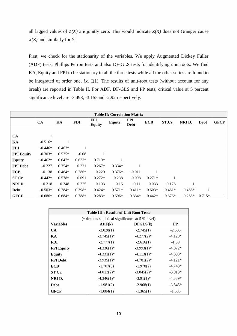
all lagged values of Z(X) are jointly zero. This would indicate Z(X) does not Granger cause

X(Z) and similarly for Y.

First, we check for the stationarity of the variables. We apply Augmented Dickey Fuller

(ADF) tests, Phillips Perron tests and also DF-GLS tests for identifying unit roots. We find

KA, Equity and FPI to be stationary in all the three tests while all the other series are found to

be integrated of order one, i.e. I(1). The results of unit-root tests (without account for any

break) are reported in Table II. For ADF, DF-GLS and PP tests, critical value at 5 percent

significance level are -3.493, -3.155and -2.92 respectively.

Table II: Correlation Matrix

CA KA FDI FPI

Equity Equity

FPI

Debt ECB ST.Cr. NRI D. Debt GFCF

CA 1

KA -0.516* 1

FDI -0.446* 0.463* 1

FPI Equity -0.303* 0.525* -0.08 1

Equity -0.462* 0.647* 0.623* 0.719* 1

FPI Debt -0.227 0.354* 0.231 0.267* 0.334* 1

ECB -0.138 0.464* 0.286* 0.229 0.376* -0.011 1

ST Cr. -0.442* 0.578* 0.091 0.272* 0.238 -0.008 0.271* 1

NRI D. -0.218 0.248 0.225 0.103 0.16 -0.11 0.033 -0.178 1

Debt -0.503* 0.784* 0.398* 0.424* 0.571* 0.411* 0.603* 0.461* 0.466* 1

GFCF -0.686* 0.684* 0.788* 0.283* 0.696* 0.334* 0.442* 0.376* 0.268* 0.715* 1

Table III : Results of Unit Root Tests

(* denotes statistical significance at 5 % level)

Variables ADF(k) DFGLS(k) PP

CA -3.028(1) -2.745(1) -2.535

KA -3.745(1)* -4.277(2)* -4.128*

FDI -2.777(1) -2.616(1) -1.59

FPI Equity -4.336(1)* -3.993(1)* -4.872*

Equity -4.331(1)* -4.113(1)* -4.393*

FPI Debt -3.935(1)* -4.781(2)* -4.121*

ECB -1.707(3) -1.978(2) -4.743*

ST Cr. -4.012(2)* -3.845(2)* -3.913*

NRI D. -4.346(1)* -3.91(1)* -4.339*

Debt -1.981(2) -2.968(1) -3.545*

GFCF -1.084(1) -1.365(1) -1.535

11

The Zivot-Andrews test showed the presence of a structural break (mainly around the global

financial crisis of 2008-09) in some of the KA components confirming plots of the indices,

which also reflect the same. The results of Zivot-Andrews one-break test are reported in

Table IV. The critical values for Zivot and Andrews test are -5.34 and -4.80 at 1 % and 5 %

levels of significance respectively.

Table IV: Result of Zivot and Andrews One-Break Test

(* denotes statistical significance at 5% level. ** denotes statistical significance at 1% level)

Variables k t statistics Break point

CA 0 -4.241 2008-09Q2

KA 2 -4.956* 2006-07Q3

FDI 1 -4.151 2006-07Q3

FPI Equity 0 -5.731** 2009-10Q1

Equity 0 -7.265** 2006-07Q3

FPI Debt 2 -5.287** 2005-06Q1

ECB 2 -4.104 2005-06Q4

ST Cr 2 -4.515 2006-07Q1

NRI D. 0 -6.312** 2011-12Q2

Debt 0 -5.054* 2005-06Q4

GFCF 0 -3.706 2012-13Q1

Table V: Lag Selection Criteria Based on AIC for VAR Modeling

Model No. Variables Lag length

I CA, GFCF, KA 5

II CA, GFCF, FDI 4

III CA, GFCF, FPI Equity 4

IV CA, GFCF, Equity 4

V CA, GFCF, FPI Debt 4

VI CA, GFCF, ECB 4

VII CA, GFCF, NRI Dep. 5

VIII CA, GFCF, ST Credit 5

IX CA, GFCF, Debt 4

To control for the structural break(s), we introduce time dummies (as exogenous variables) in

our VAR models. Also, we check for any co-integration existing between various series but

we find no series to be cointegrated.

For each VAR model, we choose appropriate lag lengths according to the Akaike Information

Criterion (AIC). Table V presents the variables in each model along with the chosen lag

length. Based on the VAR model, a Wald Test is applied where the null hypothesis is to test

12

whether the coefficients of all lagged values of Z(X) are jointly zero. This would indicate

Z(X) does not Granger cause X(Z) and similarly for Y.

5. Empirical Findings

Tables VIa-c presents the results of our analysis. There is no causality in any direction

between the KA and CA or the main debt and equity components. But all the models of Table

VI show strong causality from GFCF to the CA, implying that investment widens the CAD,

in line with theory. Both KA and CA affect GFCF, but equity and debt components do not

(Table VIa). On testing with components of KA, CA affects GFCF only in the presence of

FDI and NRI deposits (Tables VIb, c).

Table VI: Granger Causality Results

(significant results are highlighted)

Table VIa: CA, KA, KA components: equity and debt

Model Wald test null hypothesis Chi square value

Ia

KA do not GC CA 1.4

CA do not GC KA 0.12

GFCF do not GC KA 0.83

GFCF do not GC CA 5.27

KA do not GC GFCF 3.62

CA do not GC GFCF 7.22

IIa

Equity do not GC CA 1.87

CA do not GC Equity 0.38

GFCF do not GC Equity 0.18


Equity do not GC GFCF 1.41


IIIa

Debt do not GC CA 0.31

CA do not GC Debt 2

GFCF do not GC Debt 1.53


Debt do not GC GFCF 0.07


Of the KA and all its components only KA and FDI show one-way causality to the CA. Thus

there is only indirect causality from KA to CA through FDI and its impact on GFCF.

There is no causality in any direction with net equity or net FPI equity flows, implying

volatile equity flows neither deteriorate the CA nor contribute to investment (Tables VIa, b).

13

Table VIb: CA, FDI and FPI-equity


Ib

FDI do not GC CA 0.92

CA do not GC FDI 0.24

GFCF do not GC FDI 0.86


FDI do not GC GFCF 6.33


IIb

FPI Equity do not GC CA 0.45

CA do not GC FPI Equity 1.85

GFCF do not GC FPI Equity 0.44


FPI Equity do not GC GFCF 0.01


Table VIc: CA and debt components


Ic

FPI Debt do not GC CA 0.04

CA do not GC FPI Debt 12.28

GFCF do not GC FPI Debt 0.01


FPI Debt do not GC GFCF 0


IIc

ECB do not GC CA 0.35

CA do not GC ECB 1.52

GFCF do not GC ECB 2.03


ECB do not GC GFCF 0.02


IIIc

NRI Dep. do not GC CA 2.15

CA do not GC NRI Dep. 2.96

GFCF do not GC NRI Dep. 0.89


NRI Dep. do not GC GFCF 0.32


IVc

ST Cr. do not GC CA 1.74

CA do not GC ST Cr. 0.31

GFCF do not GC ST Cr. 0


ST Cr. do not GC GFCF 0.03


There is unidirectional Granger causality from the CA to FPI-debt, and also to NRI deposits,

but they were not causal for GFCF (Table VIc). This suggests that certain components of net

14

debt inflows were used to finance the CA, bridging gaps at short notice. Even so, they did not

increase GFCF10

. Of all the KA components, only FDI Granger causes GFCF (Table VIb).

FPI and its components were expected to contribute to capital formation by deepening

financial markets but the estimations do not find evidence of this.

6. Conclusion

We test for Granger causality between the CA and the KA and its various components in the

presence of GFCF. Granger causality shows if changes or imbalances in one account help

predict and therefore precede changes in the other account. To the extent KA or its

components finance GFCF they make the CA sustainable as capacity is built for the future.

The relation of KA and each of its components with the CA and GFCF could differ. Use of

disaggregated components of the KA also sidesteps possible spurious causality due to the

BOP identity at the aggregate level. The results of this analysis can help us identify

components of the BOP, which are critical for macroeconomic imbalances.

There is no direct causality in any direction between the CA and the KA. The only

component of KA which is causal for GFCF is FDI. This implies indirect causality from the

KA to the CA, since GFCF consistently affects CA. The equity components of the KA show

no causal relationship with the CA but net FPI debt inflows and net NRI deposits show one-

way causality running from the CA to them.

Overall, the findings suggest that India’s prudent gradualism on capital account

convertibility, such as caps on debt flows, may have reduced disruptions from the KA,

mitigating the developing country pattern of KA affecting the CA, while allowing use of

some components for financing the CA. Although there were less restrictions on FPI and

equity flows, which were also volatile, foreign exchange intervention and a managed float

may have prevented persistent deviations from equilibrium real exchange rate11

that could

affect the CA. Recent policy seeks to encourage FDI. Our results support this, since FDI is

10

In 2011 as the Indian CAD widened caps on debt inflows were relaxed. 11

REER shows two-way movement suggesting the absence of persistent deviation. It fell from 109.23 in 2007-

08 to 99.72 in 2008-09 (in the year of Global Financial Crisis); however it rose again to 104.97 in 2009-10.

There are varying views on the impact of REER on net exports. Cheung and Sengupta (2013) find a strong and

significant negative impact of REER appreciation on India’s export share. Goyal (2015) finds export growth to

be high even during appreciation of the REER. Veeramani (2008) finds that the degree of the (negative)

association between REER and exports has declined since 2002 for the Indian economy, so that REER changes

need not have a large effect on the CA.

15

the only KA component that affects investment, and a CAD that finances fixed investment is

sustainable, as capacity expands. India must continue its careful phased opening of the KA

account, until the domestic financial sector acquires sufficient depth to allow graduation to

the developed country pattern where causality tends to run from the CA to the KA.

References

Cheung, Y-W., and R. Sengupta. (2013). ‘Impact of exchange rate movements on exports: an

analysis of Indian non-financial sector firms.’ Journal of International Money and

Finance 39: 231-245.

Ersoy, I. (2011). ‘The causal relationship between the financial account and the current

account: the case of Turkey.’ International Research Journal of Finance and Economics 75:

187-193.

Garg, B. and K. P. Prabheesh. (2015). ‘Causal relationships between the capital account and

the current account: an empirical investigation from India.’ Applied Economics Letters 22:

446-450.

Goyal, A. (2015) ‘External shocks.’ In India Development Report, S. Mahendra Dev ed. New

Delhi: IGIDR and Oxford University Press. Available at https://mpra.ub.uni-

muenchen.de/72498/1/MPRA_paper_72498.pdf

Kim, C-H. and D. Kim. (2011). ‘Do capital inflows cause current account deficits?’ Applied

Economics Letters 18(5): 497-500.

Lau, E. and N. Fu. (2011). ‘Financial and current account interrelationship: An empirical

test.’ Journal of Applied Economic Sciences (JAES) 1(15): 34-42.

Veeramani, C. (2008). ‘Impact of exchange rate appreciation on India's exports.’ Economic and

Political Weekly 43(22): 10-14.

Yan, H-D. (2005). ‘Causal relationship between the current account and financial

account.’ International Advances in Economic Research 11(2): 149-162.

Yan, H-D. (2007). ‘Does capital mobility finance or cause a current account imbalance?’ The

Quarterly Review of Economics and Finance 47(1): 1-25.

Yan, H-D., and C-L. Yang. (2008). ‘Foreign capital inflows and the current account

imbalance: which causality direction?’ Journal of Economic Integration 23(2): 434-461.

Yan, H-D., and C-L. Yang. (2012). ‘Are there different linkages of foreign capital inflows and

the current account between industrial countries and emerging markets?’ Empirical Economics

43(1): 25-54.

estimating the relationship between the current account ... · estimating the relationship between...

Documents