1

CH7 Testing For Tradability

2

Agenda

1. Introduction2. The linear relationship3. Estimating the linear relationship: The multifactor approach4. Estimating the linear relationship: The regression approach5. Testing residual for tradability

3

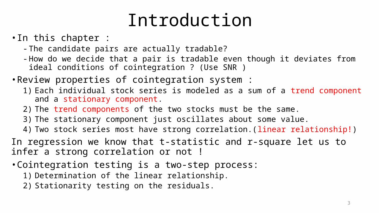
Introduction• In this chapter :

- The candidate pairs are actually tradable?- How do we decide that a pair is tradable even though it deviates from ideal conditions of

cointegration ? (Use SNR )

• Review properties of cointegration system :1) Each individual stock series is modeled as a sum of a trend component and a stationary

component.2) The trend components of the two stocks must be the same.3) The stationary component just oscillates about some value.4) Two stock series most have strong correlation.(linear relationship!)

In regression we know that t-statistic and r-square let us to infer a strong correlation or not ! • Cointegration testing is a two-step process:

1) Determination of the linear relationship.2) Stationarity testing on the residuals.

4

The linear relationship• The linear relationship between the two time series: ; : Cointegration coefficient . (CH6) : Equilibrium value . (This chapter) : Time series with zero mean .• Two approaches to estimating the equilibrium relationship:

1) The multifactor approach2) The regression approach

5

Estimating the linear relationship:The multifactor approach

• Stock B is the independent variable:

• Stock A is the independent variable:

• If we choose the largest one () mean that we choose a lower volatility one .

6

Estimating the linear relationship:The multifactor approach

• Steps of this approach: Step1: Calculate the two values and using multifactor model constructs. Step2: We choose the larger of the two values and to use for cointegration coefficient. Step3: Construct the time series corresponding to the appropriate linear combination and evaluate its mean. If it is significant, we have a nonzero equilibrium value; otherwise, it is zero.

7

Estimating the linear relationship:The regression approach

• The linear regression approach :

: response variable : control variabale

: intercept : error term

: slope So , we know if we have homoscedasticity assumption , we can easily use the OLSE method to estimate the intercept and slope by the data we have . But the stock price data really can do ?

8

Estimating the linear relationship:The regression approach

• Let us see some problems about the stock price data :1. We use just one representative value for the price in a given time period but the price

change constantly.2. There is no distinct separation of cause and effect. - In CH5 , we discussed in the error correction model for cointegration.

3. The price values are read as outputs , so we now face two output variable . It is different from regression.

We can assert that our situation is one where the uncertainty associated with each data point is different.

1 1 1

1 1 1

log( ) log( ) [log( ) log( )]

log( ) log( ) [log( ) log( )]

A A A Bt t A t t A

B B A Bt t B t t B

p p p p

p p p p

9

Estimating the linear relationship:The regression approach

• The situation of nonconstant error distributions coupled with errors in both variables can be handled by minimizing the chi-squared merit function:

and is variance of and with zero mean.

1. If the variance as shown in the denominator was a constant , then the minimization boils down to minimizing the sum of squared errors , which is the ordinary least squares procedure.

2. It can see as the sum of squared errors each normalized by its variance , so this approach to regression using the chi-squared merit function is sometimes also called the weighted least squares approach ( WLS ).

10

Estimating the linear relationship:The regression approach

• Use WLS should face some problems : 1. Weighted least squares approach assume the error only in the response variable and

not in both .2. We don’t have term in the denominator . It make the process of minimize the chi-

squared merit function need to resort to numerical methods .

So , using regression approach to solve this kind of problems is very very complicated !

11

Testing residual for tradability

• In an ideal situation for tradability , the two stocks would be cointegrated , and the residual series would be stationary .

- Mean reversion.

So It would therefore be nice if we could quantify the degree of mean reversion of a given time series.• The frequency of zero-crossing is then the number of times we can expect the time series to cross its equilibrium value in unit time.

- Time of mean reversion more short -> Time of holding position more short.

• It turns out that highly mean-reverting series are also characterized by a high frequency of zero-crossings.

12

Testing residual for tradability• How to explain Zero-crossing ?

- Arcsine law : (P. Levy) with pdf

1. T : stop time of the series g : the last time when zero is visited 2. we expect the zero crossing to have occurred with high probability only at the extremes of the time interval.

13

Testing residual for tradability• Direct method (this book tell us): 1. First, we get the sample small size population of time between crossings by counting the time between subsequent crossings in the residual series. 2. A probability distribution is then constructed by resampling repeatedly from the existing sample. The large sample obtained as a result of the resampling exercise is then used to construct the probability distribution. (Bootstrap method) 3. Percentile levels may then be constructed for the population. We can then check to see if the rates at the desired percentile levels on either side of the median satisfy our trading requirements. If they do, then we declare the pair tradable and vice versa.

14

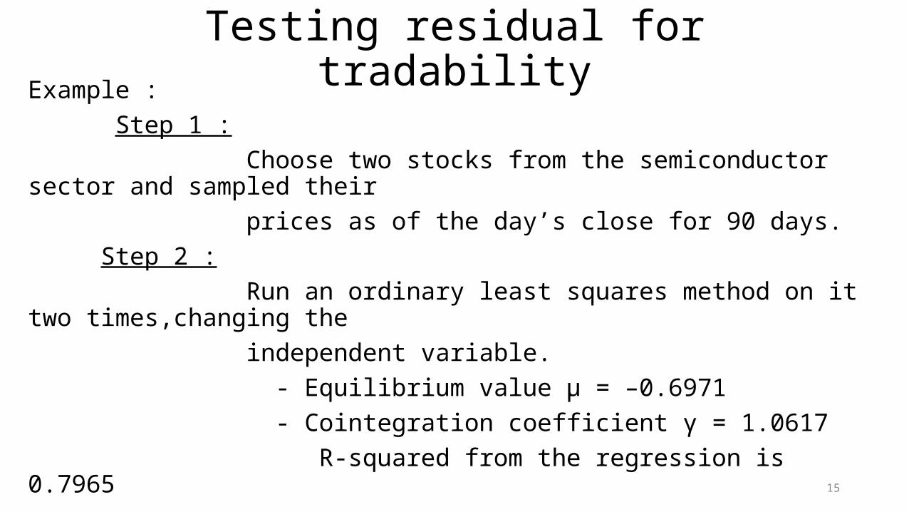
Testing residual for tradabilityExample : Step 1 : Choose two stocks from the semiconductor sector and sampled their prices as of the day’s close for 90 days. Step 2 : Run an ordinary least squares method on it two times,changing the independent variable. - Equilibrium value μ = –0.6971 - Cointegration coefficient γ = 1.0617 R-squared from the regression is 0.7965

15

Testing residual for tradabilityExample : Step 1 : Choose two stocks from the semiconductor sector and sampled their prices as of the day’s close for 90 days. Step 2 : Run an ordinary least squares method on it two times,changing the independent variable. - Equilibrium value μ = –0.6971 - Cointegration coefficient γ = 1.0617 R-squared from the regression is 0.7965

16

Testing residual for tradability

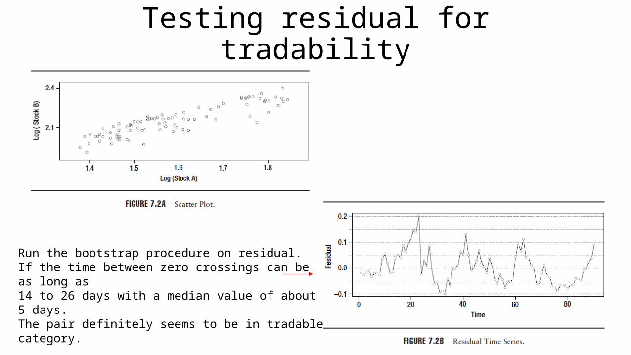
Run the bootstrap procedure on residual.If the time between zero crossings can be as long as14 to 26 days with a median value of about 5 days.The pair definitely seems to be in tradable category.

17

Some problem of this chapter

1. Why we need to select the largest ? Short a lower volatility one ?

2. Does log of price can operate directly ?