ANZIAM J. 50 (CTAC2008) pp.C598–C609, 2008 C598

Estimating the potential predictability ofWestern Australian surface temperature using

monthly data

S. Grainger1 C. S. Frederiksen2 X. Zheng3

(Received 11 August 2008; revised 16 December 2008)

Abstract

The seasonal mean of a climate variable is considered to be a statis-tical random variable with two components: a slow component relatedto slowly varying (time scales of a season or more) forcings from exter-nal and internal atmospheric sources, and an intraseasonal componentrelated to forcings from weather variability with time scales less than aseason. Here, an extension of a previous Analysis of Variance methodis proposed which deals with climate data in all seasons when esti-mating the intraseasonal variability. By removing this from the totalvariability, an estimate for the slow component, and hence the longrange predictability, of the seasonal mean is made. The method isapplied to monthly surface temperature data for Western Australiafrom 1951–2000.

http://anziamj.austms.org.au/ojs/index.php/ANZIAMJ/article/view/1414gives this article, c© Austral. Mathematical Soc. 2008. Published December 18, 2008.issn 1446-8735. (Print two pages per sheet of paper.)

Contents C599

Contents

1 Introduction C599

2 Methodology C6002.1 Statistical model . . . . . . . . . . . . . . . . . . . . . . . C6002.2 Solution for Australian surface temperature . . . . . . . . C6022.3 Potential predictability . . . . . . . . . . . . . . . . . . . . C603

3 Potential predictability of Western Australian surface tem-perature C604

4 Conclusions C607

References C608

1 Introduction

Climate variability has a major impact on the Australian economy, primarilythrough its direct impact on agriculture. Climate variability is managedthrough the provision of seasonal forecasts, the skill (or accuracy) of whichis able to be assessed (for example, Fawcett et al. [1]). This raises the issueof where efforts and funds should be directed for better understanding thelarge scale processes which the provision of skilful forecasts depend upon.In particular, what are the regions and seasons where surface climate ispotentially predictable?

Central to this question, and to seasonal forecasting, is the concept thatthe seasonal mean of a climate variable is considered to be a statistical ran-dom variable consisting of signal and noise components [2]. The signal isrelated to slowly varying (a season or more) boundary, or external, forcingsor internal atmospheric variability and is considered as the ‘slow’ component

2 Methodology C600

of interannual variability of the seasonal mean [7]. The noise is related tointernal atmospheric variability with time scales of about two weeks to aseason and has been termed the ‘intraseasonal’ component of variability [7].

Frederiksen and Zheng [2] reviewed methods to estimate the intrasea-sonal variance. Recently, a method has been formulated to estimate theintraseasonal variance from monthly mean observations [9]. However, whilethe assumptions used are probably valid for summer and winter, this is notnecessarily the case in all seasons. Here, we apply less restrictive assump-tions about the monthly statistics of climate anomalies, in order to extendthe analysis to include all seasons.

2 Methodology

2.1 Statistical model

Given the statistical model described above, the monthly mean anomaly ofa climate variable x is [2, 7, 9]

xym = µy + εym , (1)

where m (m = 1, 2, 3) is the month index in the season, y (y = 1, . . . , Y)is the year index and Y is the total number of years, µy is the seasonalpopulation mean, and εym is the monthly departure of xym from µy. Itis assumed that the vector (εy1, εy2, εy3) is a stationary and independentrandom vector with respect to year y [5]. Although µy and εym are not able tobe directly separated, it is possible to do so for their respective variances V [9]

V(xyo) = V(εyo) + V(µy) + 2V(µy, εyo) , (2)

where a subscript ‘o’ represents the average over an index (m or y).

2 Methodology C601

Here, we denote the interannual variance of εym by

V(εym) = σ2m , (3)

for each month m. The intermonthly correlations, C(εym, εyn), are thendefined as

C(εym, εyn) =V(εym, εyn)

σmσn

= φmn , m, n = 1, 2, 3 , m 6= n , (4)

where V(εym, εyn) denotes the covariance between the intraseasonal com-ponents in months m and n. The interannual variance of the intraseasonalcomponent is then

V(εyo) = E

(13

3∑m=1

εym

)2

=1

9

(σ2

1 + σ22 + σ2

3 + 2σ1σ2φ12 + 2σ2σ3φ23 + 2σ1σ3φ13

), (5)

where E denotes the expected value.

In order to estimate the terms on the right hand side of equation (5), weconsider the expectation value of the monthly differences of εym:

E

[(εy1 − εy2

εy2 − εy3

)(εy1 − εy2

εy2 − εy3

)T]

=(σ2

1 − 2σ1σ2φ12 + σ22 σ1σ2φ12 − σ1σ3φ13 − σ2

2 + σ2σ3φ23

σ1σ2φ12 − σ1σ3φ13 − σ22 + σ2σ3φ23 σ2

2 − 2σ2σ3φ23 + σ23

).

(6)

From equation (1), differences in the monthly mean are assumed to be entirelydue to the intraseasonal component (for example, xy1 − xy2 = εy1 − εy2).Hence the monthly moments of εym are defined in terms of the monthlymoments of xym:

E (εy1 − εy2)2

= E (xy1 − xy2)2 ≈ 1

Y

Y∑y=1

(xy1 − xy2)2 ≡ a , (7)

2 Methodology C602

E (εy1 − εy2) (εy2 − εy3) = E (xy1 − xy2) (xy2 − xy3)

≈ 1

Y

Y∑y=1

(xy1 − xy2) (xy2 − xy3) ≡ b , (8)

E (εy2 − εy3)2

= E (xy2 − xy3)2 ≈ 1

Y

Y∑y=1

(xy2 − xy3)2 ≡ c . (9)

From equation (6), this leads to the following set of equations

σ21 − 2σ1σ2φ12 + σ2

2 ≈ a , (10)

σ1σ2φ12 − σ1σ3φ13 − σ22 + σ2σ3φ23 ≈ b , (11)

σ22 − 2σ2σ3φ23 + σ2

3 ≈ c . (12)

2.2 Solution for Australian surface temperature

Equations (10), (11) and (12) represent three equations with six unknowns.In order to use monthly mean data, it is necessary to make some assumptionsabout the monthly statistics of the climate data. For Australian surfacetemperature, it is assumed that the standard deviation of εym varies linearlyacross a season by a parameter β:

σ1 = σ2 − β, σ3 = σ2 + β, |β| < σ2 . (13)

It is also assumed that the intermonthly correlations of εym are stationarywithin each season:

φ12 = φ23 . (14)

Grainger et al. [3] showed that the assumptions in equations (13) and (14)to a first order account for the variability of Australian surface temperaturewithin a season. Recognising that day-to-day weather events are unpre-dictable beyond a week or two, we further assume that the intraseasonalcomponents are uncorrelated if they are a month or more apart:

φ13 = 0 . (15)

2 Methodology C603

Since daily surface temperature is a first order autoregressive process, Zhenget al. [8] showed that the estimation error is reduced by applying the con-straint

0 ≤ φ12 ≤ 0.1 . (16)

Applying equations (13), (14) and (15) to equations (10), (11) and (12)leads to the following set of three equations with three unknowns:

(σ2 − β)2 − 2σ2(σ2 − β)φ12 + σ22 ≈ a , (17)

σ22(2φ12 − 1) ≈ b , (18)

(σ2 + β)2 − 2σ2(σ2 + β)φ12 + σ22 ≈ c . (19)

Equations (17), (18) and (19) are solved by rearranging to form a cubic equa-tion for φ12. The real root of the solution is then constrained by equation (16)before back-substitution into equations (17) and (19) to find β and σ2. Theintraseasonal variance is then estimated as

V̂(εyo) =1

9

[σ̂2

2(3+ 4φ̂12) + 2β̂2], (20)

where the caret ‘̂ ’ denotes an estimate.

2.3 Potential predictability

The total interannual variability of the seasonal mean of a climate variableis estimated by the sample variance

V̂(xyo) =1

Y − 1

Y∑y=1

[xyo − xoo]2. (21)

A commonly used definition of potential predictability (for example, Fred-eriksen and Zheng [2], Zheng et al. [9]) is the fraction of total interannual

3 Potential predictability of Western Australian surface temperature C604

variability of the seasonal mean that is not due to the intraseasonal variance,

Potential Predictability ≡ 1−V̂(εyo)

V̂(xyo), (22)

which is calculated using equations (20) and (21).

3 Potential predictability of Western

Australian surface temperature

To illustrate the methodology, the potential predictability of surface tem-perature for Western Australia is estimated using equation (22). Monthlymean surface maximum and minimum temperature were obtained from theAustralian Bureau of Meteorology National Climate Centre gridded histor-ical dataset [4]. Surface maximum and minimum temperature were chosenfor analysis since they are direct observations from the network of Australianweather stations. Data was obtained for period November 1950 to December2000 on a grid of 1◦ × 1◦ latitude/longitude land surface points.

The estimated potential predictability of Western Australian surface max-imum temperature for all 12 three month ‘seasons’ is shown in Figure 1 asa percentage. Each season is denoted by the first letter of each month (forexample, December–January–February is djf). North of 20◦S, there is gener-ally high potential predictability (at least 50%) throughout most of the year.However, in other regions, there is a more pronounced seasonal cycle. Forexample, potential predictability along the west coast goes from a maximum(over 60%) in jja to a minimum (less than 20%) in djf.

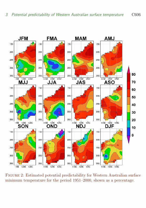
Figure 2 shows the estimated potential predictability of Western Aus-tralian surface minimum temperature. Like surface maximum temperature,the potential predictability is generally high north of 20◦S, although it is

3 Potential predictability of Western Australian surface temperature C605

Figure 1: Estimated potential predictability for Western Australian surfacemaximum temperature for the period 1951–2000, shown as a percentage.

3 Potential predictability of Western Australian surface temperature C606

Figure 2: Estimated potential predictability for Western Australian surfaceminimum temperature for the period 1951–2000, shown as a percentage.

4 Conclusions C607

much lower in ond. Elsewhere, seasonal cycles can be seen, but the struc-ture and season of these cycles differ from surface maximum temperature.For example, along the south coast potential predictability goes from lessthan 20% in jja to over 70% in ond. The different seasonal cycles are likelyto be due to differences in the processes involved with daily surface maxi-mum and minimum temperature, which have been considered in terms of thediurnal cycle of the surface energy budget [6].

4 Conclusions

An existing Analysis of Variance method has been extended to estimate theintraseasonal variance of the seasonal mean of a climate variable in all sea-sons. By making assumptions about the monthly statistics that are validfor Australian surface temperature, the intraseasonal variance, and thereforethe potential predictability, is estimated from monthly mean data for all sea-sons. The new methodology was applied to surface maximum and minimumtemperature for Western Australia for the period 1951–2000. The potentialpredictability shows distinct cycles over the 12 three month seasons. Thesecycles are different for surface maximum and minimum temperature, which islikely to be due to differences in the physical processes involved for the dailytemperature. In general, the potential predictability for surface minimumtemperature is somewhat higher than for surface maximum temperature.The sources of potential predictability will be examined in future by extend-ing to all seasons the current methodology for estimating the intraseasonalcovariance of two climate variables [7].

Acknowledgements Monthly mean surface maximum and minimum tem-perature data for Western Australia was provided by the National ClimateCentre of the Australian Bureau of Meteorology. sg is supported by theAustralian Climate Change Science Program of the Australian Department

References C608

of Climate Change. xz is supported by the New Zealand Foundation forResearch, Science and Technology (contract c01x0701). csf acknowledgesthe support of the Western Australian Department of Environment and Con-servation under the Indian Ocean Climate Initiative Stage 3.

References

[1] R. J. B. Fawcett, D. A. Jones and G. S. Beard. A verification ofpublicly issued seasonal forecasts issued by the Australian Bureau ofMeteorology: 1998–2003. Aust. Meteor. Mag., 54:1–13, 2005. C599

[2] C. S. Frederiksen and X. Zheng. Coherent Structures of InterannualVariability of the Atmospheric Circulation: The Role of IntraseasonalVariability. Frontiers in Turbulence and Coherent Structures, WorldScientific Lecture Notes in Complex Systems, Vol. 6, Eds Jim Denierand Jorgen Frederiksen, World Scientific Publications, 87–120, 2007.C599, C600, C603

[3] S. Grainger, C. S. Frederiksen and X. Zheng. Estimating the potentialpredictability of Australian surface maximum and minimumtemperature. Climate Dynamics, Accepted, 2008. C602

[4] D. A. Jones and B. C. Trewin. The spatial structure of monthlytemperature anomalies over Australia. Aust. Meteor. Mag.,49:261–276, 2000. C604

[5] E. N. Lorenz. On the existence of extended range predictability.J. Appl. Meteor., 12:543–546,doi:10.1175/1520-0450(1973)012¡0543:OTEOER¿2.0.CO;2, 1973. C600

[6] I. G. Watterson. The diurnal cycle of surface air temperature insimulated present and doubled CO2 climates. Climate Dynamics,13:533–545, doi:10.1007/s003820050181, 1997. C607

References C609

[7] X. Zheng and C. S. Frederiksen. Variability of seasonal-mean fieldsarising from intraseasonal variability. Part 1, methodology. ClimateDynamics, 23:177–191, doi:10.1007/s00382-004-0428-7, 2004. C600,C607

[8] X. Zheng, H. Nakamura and J. A. Renwick. Potential predictability ofseasonal means based on monthly time series of meteorologicalvariables. J. Climate, 13:2591–2604,doi:10.1175/1520-0442(2000)013¡2591:PPOSMB¿2.0.CO;2, 2000. C603

[9] X. Zheng, M. Sugi and C. S. Frederiksen. Interannual variability andpredictability in an ensemble of climate simulations with theMRI-JMA AGCM. J. Meteor. Soc. Jap., 82:1–18,doi:10.2151/jmsj.82.1, 2004. C600, C603

Author addresses

1. S. Grainger, Centre for Australian Weather and AtmosphericResearch, Bureau of Meteorology, GPO Box 1289, Melbourne,Victoria 3001, Australia.mailto:s.grainger@bom.gov.au

2. C. S. Frederiksen, Centre for Australian Weather and AtmosphericResearch, Bureau of Meteorology, GPO Box 1289, Melbourne,Victoria 3001, Australia.

3. X. Zheng, National Institute of Water and Atmospheric Research,Wellington, New Zealand