Estimating a War of Attrition: The Case of the U.S.

Movie Theater Industry

Online Appendix

Yuya Takahashi

January 26, 2015

Appendix A: Proofs (Online Appendix, Not for Publi-

cation)

Claim Consider a two-player game. Pick θ arbitrarily such that θ > Π2. Let T (ω, ·) be the policy

function if the two-player subgame starts at t = 0; i.e., ω = (2, 0,h0). Let Φ (t;ω) be its

inverse. For any t0 such that 0 < t0 < T (ω, θ) , let T̃ (ω′, ·) with ω′ = (2, t0,ht0) denote

another policy function. Also let Φ̃(t;ω′) be its inverse. Then, T (ω, θ) = T̃ (ω′, θ) for all

θ ≤ θ̃ where θ̃ = Φ (t0;ω) .

In other words, the optimal exit time that is planned at time zero equals the one that is planned

at some later time, conditional on nobody having exited until then.

Proof of Claim In equilibrium, at time t0, theater i knows that θj is equal to or smaller than

Φ (t0;ω) . If not, theater j would have been better off by exiting at t0 − ε, which contradicts

the construction of Φ (t0;ω) . Thus, θ̃ = Φ (t0;ω) is the highest possible value of θ of

surviving opponents and is a sufficient statistic for the history of the game up until t0. If

theater i chooses stopping time τ ≥ t0, the present discounted sum of its expected profits at

1

t0 is

V (τ , T̃−i,ω′, θi) = Pr(T̃ (ω′, θj) ≥ τ)

[∫ τ

t0

Πn (t) e−r(t−t0)dt+θire−r(τ−t0)

]+

∫{θj |T̃ (ω′,θj)<τ}

[∫ T̃ (ω′,θj)

t0

Πn (t) e−r(t−t0)dt

+e−r(T̃ (ω′,θj)−t0)V (T̃ ,ω′′, θi)]g(θj|θj ≤ θ̃)dθj,

where ω′′ = (1, T̃ (ω′, θj),hT̃ (ω′,θj)). Taking the first-order condition and rearranging gives

Φ̃′(t;ω′) = −G(Φ̃(t;ω′)|θj ≤ θ̃)

g(Φ̃(t;ω′)|θj ≤ θ̃)

[Φ̃(t;ω′)− Π2 (t)

V (T̃ ,ω′′, Φ̃(t;ω′′))− Φ̃(t;ω′)/r

]

= −G(Φ̃(t;ω′))

g(Φ̃(t;ω′))

[Φ̃(t;ω′)− Π2 (t)

V (T̃ ,ω′′, Φ̃(t;ω′′))− Φ̃(t;ω′)/r

]. (A1)

where the second equality follows fromG(Φ̃(t;ω′)|θj≤θ̃)g(Φ̃(t;ω′)|θj≤θ̃)

= G(Φ̃(t;ω′))

g(Φ̃(t;ω′)). The boundary condition

is

Φ̃(t0;ω′) = Φ(t0;ω). (A2)

Since (1) and (A1) are the same, (A2) implies

Φ̃(t;ω′) = Φ(t;ω) ∀t ≥ t0.

Equivalently, T (ω, θ) = T̃ (ω′, θ) for all θ ≤ Φ (t0;ω) .�

Value Function To characterize the value of theaters, define t∗ (θ−i) = minj 6=i{T (ω, θj)}. That

is, t∗(θ−i) gives the earliest exit time of i’s competitors. Note that I make the dependence

of t∗ on state variables and strategy implicit. If theater i chooses stopping time τ when the

state variables are given by (ω, θi) and the other theaters follow strategy T−i, the present

discounted value of i’s expected payoff is

Vi(τ ,T−i,ω, θi) = Pr(t∗(θ−i) ≥ τ)

[∫ τ

s

Πn (t) e−r(t−s)dt+θire−r(τ−s)

]+

∫{θ−i|t∗(θ−i)<τ}

[∫ t∗(θ−i)

s

Πn (t) e−r(t−s)dt

+e−r(t∗(θ−i)−s)V (T,ω′, θi)

]g(θ−i)dθ−i.

where ω′ = (n− 1, t∗(θ−i),ht∗(θ−i)) and g(θ−i) =

∏j 6=i

g(θj).

2

Proof of Lemma 2 (i) Arbitrarily pick θ ∈[ΠN−1 (0) , θ

]and let ω = (N, 0,h0). Suppose

T (ω, θ) > 0. Then, θ is the marginal type at t = T (ω, θ) that is indifferent between ex-

iting at t and exiting at (t + dt). The value of waiting until (t + dt) is the probability that

one of the opponents drops out in [t, t+ dt] conditional on it having survived until t, times

the value of entering the N − 1 player subgame. On the other hand, the cost of waiting until

(t+ dt) is {(θ − ΠN (t)) dt} , which is positive because θ ≥ ΠN−1 (0) > ΠN (0) > ΠN (t).

Since the value should be equal to the cost of waiting by assumption of the marginal type,

the value of entering the N − 1 player subgame should be positive as well.

If one of the competitors, say j, drops out in the interval, theater θ’s value of entering the subgame

depends on the exit values of other surviving competitors. Since θ is the marginal type at

T (ω, θ), however, it follows that Pr (θ < θk) = 0 for any competitor k. Otherwise, player

θk should have dropped out earlier. This implies that player θ drops out immediately after

the (N − 1)-player subgame starts. Therefore, the value of staying for theater θ should be

zero. This is a contradiction.

(ii), (iii) By the same argument as Lemma 1 of Fudenberg and Tirole (1986).�

Proof of Lemma 3 (i’) The value of exit of surviving theaters is θ∗ or lower, since the equilibrium

strategy T (ω, θ) is strictly decreasing in θ, as shown in Lemma 2. Therefore, Πn (t) is higher

than the value of exit for any surviving theater until t∗, and thus no theater will exit between

t′ and t∗.

(ii’), (iii’) By the same argument as Lemma 2.�

Expression for Beliefs Lemma 2 (ii) and Lemma 3 (ii’) allow me to describe g(θj|ht) explicitly:

g(θj|ht) =

g(θj)

Pr(T (ω,θj)≥t) T (ω, θj) ≥ t,

0 T (ω, θj) < t.

Proof of Proposition 5 In the symmetric case, a slight modification of the proof for Lemma 3 in

Fudenberg and Tirole (1986) suffices. In particular, letting Φ(t;ω) and Φ̃(t;ω) be distinct

solutions of (1), (2), and (3), I can obtain a contradiction.�

Proof of Proposition 6 A theater with θi = Φ(t;ω) does not drop out if Πn (t) is strictly larger

than its exit value. If Πn (t) = Φ(t;ω), the theater does not drop out either, because there is

3

a positive probability that some of its competitors exit in the next instant; i.e.,

Pr(Φ(t;ω) < maxj 6=i{θj} < Φ(t+ s;ω)) > 0

for all t and s > 0. Thus, Πn (t) < Φ(t;ω). Next, to show that Φ(t;ω) < Πn−1 (t) ,

suppose Φ(t;ω) = Πn−1 (t). A theater with θi = Πn−1 (t) is indifferent between staying

in and exiting. By Assumption 1, however, there is always a positive probability that every

theater stays in; i.e., Pr(max {θj}j 6=i < Πn) > 0. Therefore, theater θi = Πn−1 (t) would

be better off by dropping out at t − ε. This contradicts the construction of Φ(t;ω). Thus,

Φ(t;ω) < Πn−1 (t) .�

Appendix B: Initial Conditions Problem (Online Ap-

pendix, Not for Publication)

Formally, letting fY (y|z) be the joint density of Y ∈ RK conditional on Z = z, the initial condi-

tions problem suggests that

fθ,α (θ, α|X, n) 6= fθ,α (θ, α|X) ,

where n is the observed number of theaters in 1949 andX is a set of observable market covariates.

In addition, by assumption, we have

fθ,α (θ, α|X) = fθ (θ|X) fα (α|X)

but

fθ,α (θ, α|X, n) 6= fθ (θ|X, n) fα (α|X, n) .

Thus, I need to obtain fθ,α (θ, α|X, n) , which is generated endogenously from the game before

1949 in order to calculate the likelihood function or to simulate moments of the dynamic game

of exit. One way to address this issue is to simulate the model starting from the time when the

industry was born, and infer the distributions of θ and α that are consistent with the industry

structure in 1949. The movie theater industry, however, had a non-stationary structure in the sense

that it experienced a boom in the 1920’s and 1930’s, and afterwards faced declining demand in the

1950’s. Therefore, simulating the entire history of the industry requires one to model the life cycle

of the industry, which is beyond the scope of the paper.

4

Instead, I approximate fθ,α (θ, α|X, n) by simulation as follows. I assume that N̄ potential

players play an entry game at time zero (in 1949 in my model), and entrants play the exit game

afterwards. Specifically, each potential entrant draws its value of exit, and by comparing it with

the expected value of entry, it chooses whether or not to enter the market. For a given value of

market heterogeneity and set of exit values of all potential entrants, the entry game predicts the

number of entrants in equilibrium. Since the initial number of theaters is observed, I use the entry

game to restrict the support of market heterogeneity and exit values so that, in equilibrium, the

entry game predicts the same number of entrants as is observed. Since it is hard to characterize

such a restriction analytically, I use a simulation to approximate the joint distribution of market

heterogeneity and exit values, conditional on the observed number of entrants. This simulated

distribution can then be used as an input to simulate and solve the dynamic stage of the game.

My approach can be regarded as a reduced form of a full simulation of the entire history of the

industry. Heckman (1981) proposes introduction of an additional reduced-form equation to account

for the potential correlation between the initial state of a sample and unobservable heterogeneity,

and jointly estimates the model with the additional equation. Thus, the current approach can

also be regarded as an extended version of Heckman (1981)’s model in the context of games

with serially correlated private information. Aguirregabiria and Mira (2007) also account for the

initial conditions problem associated with market-level unobservables, but in their context private

information is iid over time and thus players are not selected samples in that aspect.

To begin, I make the following assumption:

Assumption All potential players make an entry decision simultaneously at time zero without

knowing that a war of attrition will immediately follow the entry game. That is, every player

assumes that, upon entry, it earns the same per-period payoff forever.

I use πen (m) as the payoff from entering the game when n theaters do so. The above assumption

justifies this. If theaters expect that a war of attrition will start or payoffs will change sometime in

the future, then computing the value of entry is a lot more complicated.

Remember that theater i’s optimal choice D∗i is given by

D∗i = 1{

(αm + β′Xm)E[n−δem

]≥ θi

}= 1

{(αm + β′Xm)

[∑N̄−1

k=0Pr (nm,−i = k) (k + 1)−δ

]≥ θi

}(1)

5

where N̄ is the number of potential entrants and nm,−i is the number of entrants aside from i. Let

P denote a theater’s subjective probability that a competitor enters the market. By the binomial

theorem, we have

Pr (nm,−i = k) =

(N̄ − 1

k

)P k (1− P )N̄−k−1 .

Finally, (1) implies

Pr (D∗i = 1) = G

((αm + β′Xm)

[∑N̄−1

k=0

(N̄ − 1

k

)P k (1− P )N̄−k−1 (k + 1)−δ

]).

In equilibrium, the beliefs are consistent with the strategies, meaning that

P = G ((αm + β′Xm)K (P )) (2)

where

K(P ) =∑N̄−1

k=0

(N̄ − 1

k

)P k (1− P )N̄−k−1 (k + 1)−δ .

Letting P ∗ (Xm, αm) denote the unique fixed point of (2), the number of entrants predicted by

this entry model equals the number of θis in {θ1, ..., θN̄} that satisfy

(αm + β′Xm)K (P ∗ (Xm, αm))− θi ≥ 0. (3)

B.1: Simulating the Joint Distributions of α and θs

This subsection explains how the entry model is used to approximate the joint distributions of θ

and α conditional on X and n. Let Fθ,α (θ, α|X,n) be the CDF of the density fθ,α (θ, α|X,n).

Based on the entry model, I simulate the joint distribution of θ and α conditional on (Xm, nm) in

the following way:

Step 1: Draw α0 from N (0, σ2α) .

Step 2: Calculate P ∗ (Xm, α0) using (2). Then, define θ∗ as

θ∗ =(α0 + β′Xm

)K(P ∗(Xm, α

0)).

That is, θ∗ is the threshold of exit values below which a theater finds it profitable to enter the

game.

6

Step 3: Draw a value of exit nm times from TN (0, σ2θ; lθ, θ

∗) and N̄−nm times from TN (0, σ2θ; θ∗, hθ) ,

where TN(µ, σ2; a, b) denotes the truncated normal distribution with mean µ, variance σ2,

and lower and upper bounds of a and b. Sort these values in an ascending order. Call them

θ0 =(θ0

1, ..., θ0nm , θ

0nm+1, ..., θ

0N̄

).

Step 4: Define αl and αh such that

θ0nm = (αl + β′Xm)K (P ∗ (Xm, αl))

θ0nm+1 = (αh + β′Xm)K (P ∗ (Xm, αh)) .

Step 5: Draw α1 from TN (0, σ2α;αl, αh) .

That is, α1 is large enough to support entry of nm theaters but not enough to support entry of

nm + 1 theaters.

Step 6: Return to Step 2 and repeat these steps J times to get(θj, αj

)Jj=1

.1 Call this F̂θ,α|Xm,nm .

Note that this procedure is completed for each market. Any random draw (θ, α) from F̂θ,α|Xm,nm

supports exactly nm entrants in a symmetric equilibrium of the entry game.

B.2: Role of Initial Conditions

If a market has a high unobservable demand shifter, we would observe more firms in the market

than otherwise. If one were to ignore the unobservables in such a case, one would underestimate

the negative effect of competition, since many firms appear to be able to operate profitably. On the

other hand, if the unobservable demand shifter is low, the number of competitors would be small.

In such a case, one would infer that the effect of competition is strong. Furthermore, ignoring the

initial conditions problem affects estimates of other parameters as well.

To see the role of the initial conditions problem, I estimate the model using the ex-ante distri-

butions of market level heterogeneity and exit values; i.e., I use Fθ,α|nm instead of F̂θ,α|nm . Note

that the entry stage is used only for identifying the parameters in the payoff function. I have 27

moments to estimate 15 parameters.2 Table B1 shows the parameter estimates. The effect of com-

1I discard the first 30 sets of(θj , αj

)before storing.

2Compared to the full model, the average number of entrants E(nm) is excluded from the set of moments for the

following reason. Since the mean of αm is ex-ante zero, the exit game predicts too many exits at t = 0 for markets

with many competitors, unless the mean profit is very high. If the mean profit is high, however, the entry stage predicts

too many entrants.

7

petition in the dynamic game, δ, is estimated to be smaller than the full model, while that in the

entry game, δe, is larger. Thus, ignoring the initial conditions problem significantly changes esti-

mates of competition effects. The estimates of the variance of market-level heterogeneity are also

different between the two specifications.

To investigate the model fit, I simulate the model ten times and for each simulation calculate

the rate of exit during the sample period. Then, I take average over simulation draws for different

market structures. The rate of exit in monopoly markets is 9.5% in the data, while the prediction

by the model is 9.6%. In duopoly or triopoly markets, the empirical and predicted exit rates are

14.4% and 12.4%, respectively. The corresponding numbers for markets with four or five theaters

are 19.7% and 17.1%, respectively. Finally, in markets with more than five theaters, the rate of exit

in the data is 21.6%, while the prediction of the model is 20.6%.

It is difficult, however, to evaluate the importance of initial conditions, since parameters in the

payoff function are reduced-form parameters.3 To better understand the role of initial conditions, I

first simulate the model starting from 1949 until 1955, using the ex-ante distribution of unobserv-

ables.4 To fix observable variables, I only use Steuben county in Indiana for the simulation, as the

TV penetration rate in 1955 and the total population in 1950 are close to the median values in the

sample.5 Then, I assume 1955 is the “initial” period of my hypothetical sample. Put differently,

I assume that the industry was born in 1949 and the data are available from 1955. Panel (a) in

Figure B1 plots the distribution of market-level heterogeneity (α) conditional on the number of

surviving theaters in 1955. This result clearly shows that fα (α|X, n) 6= fα (α|X) . Next, I sim-

ulate F̂θ,α|Xm,nm using the simulation method proposed above, and integrate over θ to calculate

f̂α (α|X, n) for n = 3. Panel (b) in Figure B1 plots this and compares it with the true distribution

of α conditional on n = 3, which I already showed in panel (a), along with the ex-ante distrib-

ution of α. The “true” distribution of α is closer to the simulated distribution than to the ex-ante

3Another reason is that I use the entry model not only for addressing the initial condition problem but also for

identifying parameters in the base demand. One alternative would be to identify all the parameters from “dynamic”

moments only, and to use the entry model only for addressing the initial condition problem. Then, I would be able to

compare the estimation results with and without the entry model. I did not use this strategy because the correlations

between exit rates andXm are weak in the data, and thus I would not identify β in the base demand well.4Throughout this exercise, I fix σ2α = 0.6 to facilitate comparisons. Other parameters are set at the estimated

values.5The TV penetration rate in 1955 and the total population in 1950 of Steuben county are 0.54 and 17,087, respec-

tively. The median value for each variable is 0.54 and 17,150, respectively. The number of theaters in 1949 in this

county was three in the data, but I start from four theaters to have more variations in the number of theaters in 1955.

8

distribution.

Since unobservable exit values are time-invariant, selection based on exit values may be sub-

stantial too. In panel (c) in Figure B1, I plot the distribution of exit values when the industry was

born in this exercise (i.e., ex-ante distribution) and the distribution of exit values of surviving the-

aters in 1955. As expected, these two distributions are significantly different from one another.

In particular, the distribution of survivors’ exit values has a high density at the low end compared

to the unconditional distribution. I also calculated f̂θ (θ|X, n = 3) for surviving theaters in 1955,

using the proposed simulation method. Panel (c) plots this distribution. Again, the simulated dis-

tribution is closer to the true distribution of exit values of surviving theaters. Although these two

distributions are still different, it can be seen that the proposed method, to some extent, alleviates

the initial conditions problem.

One caveat is that in this exercise the game played by the theaters before the “initial” period

(i.e., 1955) is the exit game in which the payoff function is very similar to that of the entry game.

As I discussed above, in the current application, the type of game that was played before 1949

may have been different from the exit game. If the game before the initial period were, however,

different, the parameter estimates in the entry game would change accordingly, and hence be able

to capture the correlation between n, θ, and α.

References

[1] Aguirregabiria, Victor, and Pedro Mira. 2007. “Sequential Estimation of Dynamic Discrete

Games.” Econometrica, 75 (1): 1-53.

[2] Heckman, James J. 1981. “The Incidental Parameters Problem and the Problem of Initial

Conditions in Estimating a Discrete Time-Discrete Data Stochastic Process and Some Monte

Carlo Evidence.” In Structural Analysis of Discrete Data With Econometric Applications,

edited by Charles F. Manski and Daniel L. McFadden, 179-195. Cambridge: The M.I.T. Press.

9

Appendix C: Interpolation of TV Penetration Rates (Online Ap-

pendix, Not for Publication)

The TV penetration rate is reported once in 1950 and afterwards every year starting from 1953. I

use data from all available years up to 1960 to approximate the TV diffusion process by the CDF

of the Weibull distribution. For market m, I observe

(TVm1950, TVm1953, TVm1954, ..., TVm1960) .

Using 1949 as the reference year, let

T̂ V mt (k1, k2) = 1− e−((t−1949)/k1)k2 .

Then, I choose (k1, k2) to minimize∑t=1950,1953,...,1960

(TVmt − T̂ V mt (k1, k2))2

for each market. Once the minimizers are obtained, I can calculate T̂ V mt(k̂1, k̂2) for all t ∈[1949, 1955] .

This approach has several advantages. First, the interpolated TV penetration rate is continu-

ous and smooth. Linear interpolation would generate many kinks, which may not be natural in

the continuous-time model. Second, this method ensures that the theater’s payoff is monotonic,

which satisfies Assumption 1 (i). In 84 markets (about 3% of all markets), the TV penetration rate

decreases slightly from one year to another. This is most likely due to mis-measurement. I do

not need to discard these observations. Third, this method enables me to exploit information after

1955. Given that the TV penetration rate is missing in 1951 and 1952, such additional information

is valuable.

Appendix D: Importance of Movie Theater Chains (Online Ap-

pendix, Not for Publication)

Movie theater chains existed in the sample period, although their influence and market power were

much more limited compared to later periods. Unfortunately, comprehensive information on movie

theater chains in the time period of this study is not available. The Film Daily Yearbook of Motion

10

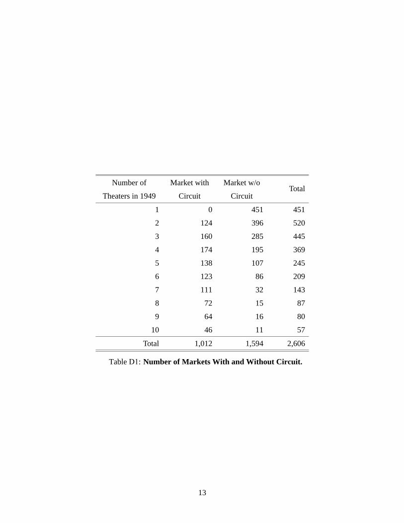
Pictures, however, lists all theaters owned by big theater chains (circuits); i.e., theater chains that

own at least four theaters in the U.S. I collect markets in which at least two movie theaters are

owned by the same theater chain and call them “market with circuit”. The remaining markets are

called “market without circuit”. In other words, in these markets, any two theaters in the market

are not owned by the same theater chain. It could still be the case that two theaters are owned by

two different chains. Table D1 shows the frequency of these markets. The majority of markets do

not have a circuit that owns more than one theater in the same market.

To further investigate if this may distort my results, I construct a dummy variable defined as

whether the market is a “market with circuit” or not, and regress the market-level exit rate on the

dummy variable as well as on the initial number of competitors, its squared term, the change in

the TV rate, the change in the population, and the number of new entrants in the market. The

sign of the coefficient of the dummy variable is positive, but not statistically significant. If theaters

under the same ownership coordinate, there would be no strategic delay and the exit rate would be

higher. In this sense, the sign of the coefficient is consistent with the argument that competition

delays exits. There is no evidence, however, that “market with circuit” significantly distort the

result. This should not be taken as evidence that chains are not important, as (i) this additional data

contain only big theater chains, and (ii) the explanatory power of the linear regression is limited.

Rather, the delay and cost of asymmetric information in this paper can be interpreted as their lower

bounds, as coordination would hasten exits.

Appendix E: Numerical Solution (Online Appendix, Not for Pub-

lication)

To solve this differential equation, the method of forward shooting cannot be used because the

problem is ill-defined at zero. The standard backward-shooting method does not work either, as

a finite end point does not exist. To deal with this issue, I apply the following algorithm. I start

from an arbitrary point t′ > 0 and use backward shooting from t′ to 0. Then, for ω = (n, 0,h0), I

choose Φ (t′;ω) such that Φ(0;ω) = Πn−1 (0) . Then, for an arbitrary ε > 0, I confirm that there

exists t′′ such that |Φ(t′′;ω)− Πn (t′′) | < ε.

11

Parameters Coef. Std. Err

δ (competition in dynamic game) 0.2009 0.1050

δe (competition in entry game) 2.1173 0.2285

β0 (constant) 8.7248 1.8764

β1 (population) 0.0687 4.3860

β2 (median age) 2.5228 1.5975

β3 (median income) 0.0206 4.0410

β4 (urban share) -2.5481 1.1484

β5 (employment share) 2.7038 1.0338

β6 (log of land area) -2.7572 1.3948

λ1 (TV rate) 0.5487 0.0596

λ2 (change in population) -3.3260 0.8608

λ3 (new entrants) 0.4326 0.1257

σθ (std. of exit value) 2.7545 0.5959

σα (std. of demand shifter) 1.8622 0.5057

ραλ (corr coef. b/w αm and λm) 0.3320 0.0861

Table B1: Estimates of Structural Parameters without Correcting the Initial

Conditions Problem.

12

Number of

Theaters in 1949

Market with

Circuit

Market w/o

CircuitTotal

1 0 451 451

2 124 396 520

3 160 285 445

4 174 195 369

5 138 107 245

6 123 86 209

7 111 32 143

8 72 15 87

9 64 16 80

10 46 11 57

Total 1,012 1,594 2,606

Table D1: Number of Markets With and Without Circuit.

13

Figure B1 Importance of Initial Condition Problem

Note: I simulate the model many times starting from 1949 until 1955, using the ex-ante distributions of unobservables. I fix observable covariates at the level of the median county. Panel (a) plots the distribution of market-level heterogeneity, splitting the simulated outcomes according to the number of surviving theaters in 1955. Then, assuming that 1955 is the initial period of my hypothetical sample, I simulate the distribution of market-level heterogeneity for n =3, using the method I discribed in Section B.1. Penel (b) plots the resulting distribution and the distribution conditional on n =3 from panel (a), along with its ex-ante distribution. Finally, panel (c) plots the ex-ante , conditional (on survival in 1955), and simulated distributions of exit values, which I obtained from the above simulation.

0

0.2

0.4

0.6

0.8

1

1.2

1.4

-3.0

0

-2.8

2

-2.6

4

-2.4

6

-2.2

8

-2.1

0

-1.9

2

-1.7

4

-1.5

6

-1.3

8

-1.2

0

-1.0

2

-0.8

4

-0.6

6

-0.4

8

-0.3

0

-0.1

2

0.06

0.24

0.42

0.60

0.78

0.96

1.14

1.32

1.50

1.68

1.86

2.04

2.22

2.40

2.58

2.76

2.94

Panel (a): Distribution of Market-Level Heterogeneity Conditional on the Number of Competitors

n=1 n=2 n=3

00.10.20.30.40.50.60.70.8

-3.0

0

-2.8

2

-2.6

4

-2.4

6

-2.2

8

-2.1

0

-1.9

2

-1.7

4

-1.5

6

-1.3

8

-1.2

0

-1.0

2

-0.8

4

-0.6

6

-0.4

8

-0.3

0

-0.1

2

0.06

0.24

0.42

0.60

0.78

0.96

1.14

1.32

1.50

1.68

1.86

2.04

2.22

2.40

2.58

2.76

2.94

Panel (b): Ex-ante, Actual and Simulated Distributions of Market-Level Heterogeneity when n=3

Ex-ante Actual Simulated

0

0.5

1

1.5

2

0.00

0.09

0.18

0.27

0.36

0.45

0.54

0.63

0.72

0.81

0.90

0.99

1.08

1.17

1.26

1.35

1.44

1.53

1.62

1.71

1.80

1.89

1.98

2.07

2.16

2.25

2.34

2.43

2.52

2.61

2.70

2.79

2.88

2.97

Panel (c): Ex-ante, Conditional (on survival), and Simulated Distribution of Exit Values

Ex-ante Conditional on survival Simulated

14