estimates of turbulent diffusivities and energy dissipation rates from

Atmos. Chem. Phys., 13, 12107–12116, 2013www.atmos-chem-phys.net/13/12107/2013/doi:10.5194/acp-13-12107-2013© Author(s) 2013. CC Attribution 3.0 License.

Atmospheric Chemistry

and PhysicsO

pen Access

Estimates of turbulent diffusivities and energy dissipation ratesfrom satellite measurements of spectra of stratospheric refractivityperturbations

N. M. Gavrilov

Atmospheric Physics Department, Saint-Petersburg State University, St. Petersburg, Russia

Correspondence to:N. M. Gavrilov ([email protected])

Received: 10 June 2013 – Published in Atmos. Chem. Phys. Discuss.: 5 July 2013Revised: 5 November 2013 – Accepted: 10 November 2013 – Published: 13 December 2013

Abstract. Approaches for estimations of effective turbu-lent diffusion and energetic parameters from characteris-tics of anisotropic and isotropic spectra of perturbationsof atmospheric refractivity, density and temperature aredeveloped. The approaches are applied to the data ob-tained with the GOMOS instrument for measurements ofstellar scintillations on-board the Envisat satellite to es-timate turbulent Thorpe scales,LT , diffusivities, K, andenergy dissipation rates,ε, in the stratosphere. At lowlatitudes, effective values areLT ∼ 1–1.1 m, ε ∼ (1.8–2.4)× 10−5 W kg−1, andK ∼ (1.2–1.6)× 10−2 m2 s−1 at al-titudes of 30–45 km in September–November 2004, de-pending on different assumed values of parameters ofanisotropic and isotropic spectra. Respective standard devi-ations of individual values, including all kinds of variabil-ity, areδLT ∼ 0.6–0.7 m,δε ∼ (2.3–3.5)× 10−5 W kg−1, andδK ∼ (1.7–2.6)× 10−2 m2 s−1. These values correspond tohigh-resolution balloon measurements of turbulent charac-teristics in the stratosphere, and to previous satellite stellarscintillation measurements. Distributions of turbulent char-acteristics at altitudes of 30–45 km in low latitudes have max-ima at longitudes corresponding to regions of increased grav-ity wave dissipation over locations of stronger convection.Correlations between parameters of anisotropic and isotropicspectra are evaluated.

1 Introduction

Internal gravity waves (IGWs) with energy propagating up-wards are important for dynamical processes and mixing inthe middle atmosphere (Fritts and Alexander, 2003). Break-ing IGWs produce turbulent mixing and kinetic energy dis-sipation and effectively influence the global circulation andcomposition in the middle atmosphere.

IGW studies use different in situ, ground-based and satel-lite measurements (Fritts and Alexander, 2003; Wu et al.,2006; Alexander et al., 2010). Key advantages of satellitemeasurements are their global coverage. To examine atmo-spheric mesoscale variations, Fetzer and Gille (1994) usedsatellite data of LIMS (Limb Infrared Monitor of the Strato-sphere). Eckermann and Preusse (1999) presented the re-sults of data processing of the satellite CRISTA (Cryo-genic Infrared Spectrometer and Telescopes for the atmo-sphere) experiment. Wu and Waters (1996) and McLan-dress et al. (2000) studied mesoscale temperature pertur-bations and obtained their global distribution in the strato-sphere and mesosphere from the data of MLS (MicrowaveLimb Sounder) instrument on-board the satellite UARS.Extensive information on atmospheric mesoscale fluctua-tions were given by the GPS/Microlab satellite (Tsuda etal., 2000; Alexander et al., 2002; Gavrilov et al., 2004;Gavrilov and Karpova, 2004). Studies of mesoscale varia-tions using a GPS radio occultation technique were contin-ued with satellite CHAMP launched in April 2001, and laterwith COSMIC group of satellites launched in 2006 (Schmidtet al., 2008; Alexander et al., 2008; Wang and Alexander,2010). Ern et al. (2004, 2011) obtained global distributionsof IGW momentum fluxes in the middle atmosphere from

Published by Copernicus Publications on behalf of the European Geosciences Union.

12108 N. M. Gavrilov: Turbulent diffusivities and energy dissipation rates in the stratosphere

global temperature measurements with the satellite instru-ments High Resolution Dynamics Limb Sounder (HIRDLS)and Sounding of the Atmosphere using Broadband EmissionRadiometry (SABER).

Recent observations of stellar scintillations from satellites(Gurvich and Kan, 2003a, b; Sofieva et al., 2007, 2009, 2010)provided new information about small-scale perturbations inthe stratosphere. The intensity of stellar light going throughthe atmosphere fluctuates (oscillates), when a satellite ob-serves a star. Relative intensity fluctuations can be as strongas several hundred percent (see Sofieva et al., 2010). Thesescintillations are due to air temperature and density irregu-larities produced by IGWs, turbulence and different instabil-ities, which produce perturbations of atmospheric refractiv-ity. The smallest scales measurable by an optical scintillationmethod may be less than a meter. Scintillation measurementsprovide information about IGW-breaking and turbulence inthe stratosphere.

First measurements of stellar scintillations with the Rus-sian space stations Salyut and Mir provided spectral andstatistical characteristics of perturbations (Gurvich et al.,2001), and also confirmed the theory of scintillations (Gur-vich and Brekhovskikh, 2001). These measurements also al-lowed determinations of IGW and turbulence spectra charac-teristics (Gurvich and Kan, 2003a, b; Gurvich and Chunchu-zov, 2003).

Multi-year measurements were performed with the GlobalOzone Monitoring by Occultation of Stars (GOMOS) instru-ment from the Envisat satellite (Bertaux et al., 2010). GO-MOS contains two photometers recording stellar light at asampling frequency of 1 kHz synchronously in 473–527 nmand 646–698 nm spectral bands during star sets behind theEarth’s limb. These measurements were used to estimate pa-rameters of anisotropic and isotropic spectra of temperatureperturbations produced by IGWs and small-scale turbulencein the stratosphere (Gurvich and Kan, 2003a; Sofieva et al.,2007, 2009, 2010).

In this paper, we developed approaches to use these spec-tral parameters for estimating turbulent kinetic energy dis-sipation rates and turbulent diffusivities produced by small-scale isotropic turbulence. We estimated the mentioned tur-bulent characteristics at altitudes of 30–45 km in September–November 2004 at latitudes 20◦ S–20◦ N and in January 2005at middle latitudes 34–36◦ N and compared them with avail-able satellite, balloon and high-resolution radiosonde data.

2 Atmospheric perturbation spectra

Sofieva et al. (2007, 2009) estimated scales of isotropic andanisotropic parts of atmospheric perturbation spectra usingobservations of stellar scintillations with the GOMOS instru-ment on-board the Envisat satellite. Scintillations producedby density perturbations along the light path give infor-mation about small-scale atmospheric dynamics (Tatarskii,

1971). Sofieva et al. (2007, 2009) considered structures ofrelative fluctuationsν = N ′

r / Nr ≈ −T ′ / T̄ of refractivityNr

and temperatureT (overbars and primes denote the statisti-cal means and perturbations, respectively). These structurescould be described with the three-dimensional spectral den-sity function8ν(k), wherek is the wave vector with com-ponents (kx , ky , kz) along horizontal axesx, y and verticalaxisz, respectively. Gurvich and Kan (2003a) and Sofieva etal. (2007) approximated8ν with a sum

8ν = 8W + 8K , (1)

where8W and8K are statistically independent anisotropicand isotropic components, respectively. The component8W

corresponds to anisotropic perturbations, produced, for ex-ample, by random IGWs (Smith et al., 1987). Gurvich andKan (2003a) and Sofieva et al. (2007) approximated thisthree-dimensional spectrum as

8W (ka) = CWη2(k2a + k2

0)−5/2φ(ka /kW ), (2)

k2a = η2k2

h + k2z ;k

2h = k2

x + k2y,

whereCW andk0 are parameters,η is the anisotropy coeffi-cient, and the functionφ(k/kW ) describes the decay of8W

at k > kW . Integration of Eq. (2) gives the one-dimensionalvertical spectrumVW (kz):

VW (kz) =

∞∫−∞

∞∫−∞

8W (ka)dkxdky ≈2π

3CW (k2

z + k20)−3/2. (3)

This expression does not depend on the anisotropy coeffi-cientη. At kz � k0 the spectrum (Eq. 3) corresponds to thek−3z slope known for saturated IGWs (Smith et al., 1987). As

far asVW (−kz) = VW (kz), one can use the symmetric one-dimension spectrum, (see Monin and Yaglom, 1975, §12)

EW (|kz|) = 2VW (kz) =4π

3CW (k2

z + k20)−3/2. (4)

The second component,8K , in Eq. (1) corresponds toisotropic turbulent irregularities produced by breaking IGWsand by other sources. Gurvich and Kan (2003a) and Sofievaet al. (2007) used a theory of locally isotropic turbulence,which gives

8K(k) = 0.033CKk−11/3exp[−(k/kK)2];k2

= k2h + k2

z , (5)

wherekK is a parameter,CK is the structure characteristic ofthe random refractivity field (see Monin and Yaglom, 1975,§23). The isotropic one-dimension spectrumEK(|kz|) can beobtained by integration of the locally isotropic spectrum8K

(see Monin and Yaglom. 1975, §21), and at|kz| � kK hasthe following form:

EK(|kz|) ≈ 0.25CK |kz|−5/3, (6)

which corresponds to the known−5/3 power law for Kol-mogorov’s turbulence (see Monin and Yaglom, 1975, §21).

Atmos. Chem. Phys., 13, 12107–12116, 2013 www.atmos-chem-phys.net/13/12107/2013/

N. M. Gavrilov: Turbulent diffusivities and energy dissipation rates in the stratosphere 12109

The structure functionDT (r) of the locally isotropic temper-ature field at displacementsr (Tatarskii, 1971) has the form

DT (r) = [T (z + r) − T (z)]2 = C2T r2/3, (7)

whereC2T is the structure characteristic of the temperature

field. According to Monin and Yaglom (1975, §13.3) for lo-cally isotropic turbulence

DT (r) = 2

∞∫0

(1− cosk′r)EK(k′)dk′= CK T̄ 2r2/3. (8)

Comparing in Eqs. (7) and (8), one can get

CK = C2T / T̄ 2. (9)

Sofieva et al. (2007, 2009) developed algorithms for estimat-ing the four parameters of anisotropic and isotropic spectra(Eqs. 2–6): the structure characteristicsCK and CW , andwavenumberskW and k0, which correspond to inner andouter scales of the anisotropic spectrum (Eq. 2). These algo-rithms were used to obtain these four parameters from obser-vations of stellar scintillations with the GOMOS instrumenton-board the Envisat satellite (Sofieva et al., 2007, 2009).

3 Estimation of turbulence characteristics

In Sect. 3.1 below, we obtain formulae connecting turbu-lent energy dissipation rates, diffusivities and other turbulentcharacteristics with parameters of anisotropic and isotropicparts of atmospheric perturbation spectra (Eqs. 4, 6). We usethese formulae for estimations of turbulent characteristics inthe stratosphere from GOMOS satellite data in Sect. 3.2. Pos-sible correlations between anisotropic and isotropic spectralparameters are considered in Sect. 3.3.

3.1 Relations between turbulent and spectralcharacteristics

Some theories of turbulent spectra (for example, Lumley,1964) introduce the “buoyancy” wavenumberkb for thecrossover between vertical anisotropic (Eq. 4) and isotropic(Eq. 6) spectral regimes,EW (kb) = EK(kb) so that

kb ≈ (16.8CW /CK)3/4. (10)

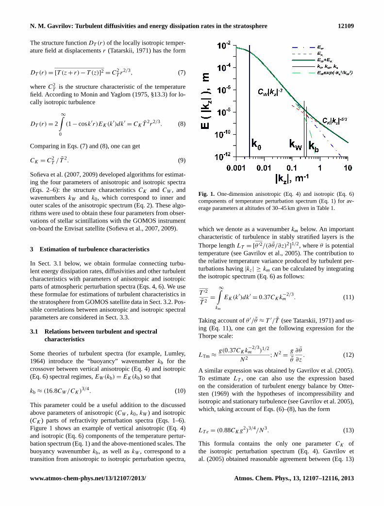
This parameter could be a useful addition to the discussedabove parameters of anisotropic (CW , k0, kW ) and isotropic(CK ) parts of refractivity perturbation spectra (Eqs. 1–6).Figure 1 shows an example of vertical anisotropic (Eq. 4)and isotropic (Eq. 6) components of the temperature pertur-bation spectrum (Eq. 1) and the above-mentioned scales. Thebuoyancy wavenumberkb, as well askW , correspond to atransition from anisotropic to isotropic perturbation spectra,

Fig. 1. One-dimension anisotropic (Eq. 4) and isotropic (Eq. 6)components of temperature perturbation spectrum (Eq. 1) for av-erage parameters at altitudes of 30–45 km given in Table 1.

which we denote as a wavenumberkm below. An importantcharacteristic of turbulence in stably stratified layers is theThorpe lengthLT = [θ ′2/(∂θ̄/∂z)2

]1/2, whereθ is potential

temperature (see Gavrilov et al., 2005). The contribution tothe relative temperature variance produced by turbulent per-turbations having|kz| ≥ km can be calculated by integratingthe isotropic spectrum (Eq. 6) as follows:

T ′2

T̄ 2=

∞∫km

EK(k′)dk′= 0.37CKk

−2/3m . (11)

Taking account ofθ ′/θ̄ ≈ T ′/T̄ (see Tatarskii, 1971) and us-ing (Eq. 11), one can get the following expression for theThorpe scale:

LTm ≈g(0.37CKk

−2/3m )1/2

N2;N2

=g

θ̄

∂θ̄

∂z. (12)

A similar expression was obtained by Gavrilov et al. (2005).To estimateLT , one can also use the expression basedon the consideration of turbulent energy balance by Otter-sten (1969) with the hypotheses of incompressibility andisotropic and stationary turbulence (see Gavrilov et al. 2005),which, taking account of Eqs. (6)–(8), has the form

LT e = (0.88CKg2)3/4/N3. (13)

This formula contains the only one parameterCK ofthe isotropic perturbation spectrum (Eq. 4). Gavrilov etal. (2005) obtained reasonable agreement between (Eq. 13)

www.atmos-chem-phys.net/13/12107/2013/ Atmos. Chem. Phys., 13, 12107–12116, 2013


and direct measurements ofLT from the data of high-resolution MUTSI balloon measurements in the troposphereand stratosphere. For steady-state turbulence, energy dissi-pation rate,ε, and turbulent diffusivity,K, are related to theOzmidov scale,LO, by

ε ≈ L2ON3

;K ≈ βL2ON, (14)

whereβ is a constant. According to a review by Fukao etal. (1994),β may vary between 0.2 and 1. The frequentlyused approximationβ =Rf/(1−Rf), where Rf is the fluxRichardson number, often taken asRf ≈ 0.25, givesβ ≈ 1/3.AssumingLO = cLT , Caldwell (1983), and more recently,Galbraith and Kelley (1996), also Fer et al. (2004) proposedthe following formulae for estimations ofε andK:

ε ≈ (cLT )2N3;K ≈ β(cLT )2N. (15)

Values of the empirical constantc vary in different studies(see discussions by Gavrilov et al., 2005 and Clayson andKantha, 2008). After Gavrilov et al. (2005), considering theresult given by Alisse (1999) for stratospheric data, we belowusec = 1.15 andβ = 1/3. Formulae Eqs. (15) and (10), (12)or (13) one can use for estimations ofLT , ε andK dependingon a set of spectral parameters available experimentally. Inthe case of GOMOS scintillation observations, we have theentire set of parametersCW , k0, kW andCK , which is enoughfor the usage of any combinations of formulae (Eqs. 10–15).This allows us to compare the results obtained with differentapproaches using Eqs. (15) and (10), (12) or (13) in the nextsection.

3.2 Turbulent diffusivities and energy dissipation rates

The methods of estimating the parametersCW , k0, kW ofanisotropic (Eq. 2) andCK of isotropic (Eq. 5) spectra of at-mospheric temperature perturbations from GOMOS satelliteobservations of star scintillations were described by Sofievaet al. (2007, 2009, 2010). The retrieval uses the standardmaximum-likelihood method with a combination of non-linear and linear optimization. The authors made nonlin-ear fits of two parametersk0 andkW using the Levenberg–Marquardt algorithm (Press et al., 1992). The parametersCK andCW were calculated with the linear weighted least-squares method. Atmospheric parameters required for thespectral parameter retrievals are taken from the ECMWFmeteorological reanalysis model. Sofieva et al. (2007, 2009,2010) presented examples of the experimental scintillationspectrums. Usually, experimental scintillations agree to theproposed modeled scintillation spectra, but sometimes peaks,possibly related to quasi-periodic disturbances in the atmo-sphere, may occur and special filtering of these peaks wasapplied by Sofieva et al. (2007, 2009, 2010).

In the present paper, we use two sets of four parametersCW , k0, CK and kW from GOMOS scintillation measure-ments by Sofieva et al. (2007, 2009, 2010). The first set in-cludes data obtained for occultations of the brightest stars

Sirius and Canopus in September–November 2004 at lati-tudes between 20◦ N and 20◦ S, which give the highest sig-nal to noise ratios. We selected four groups of measurementsat altitudes within 3 km-thick layers centered at 30, 35, 40and 45 km altitudes. The second set of analyzed data is theCanopus occultations for January 2005 at 30 km altitude andlatitudes 34–36◦ N, which allows comparisons with high-resolution radiosonde turbulence measurements by Claysonand Kantha (2008). The method by Sofieva et al. (2007, 2009,2010) also gives estimations of errors of the spectral param-eters. In the present study, we used values of spectral param-eters having relative errors smaller than 50 %. Table 1 showsthe numbers of measurementsn used in our analysis in eachaltitude layer and data set.

For each set of measured parametersCW andCK , usingEq. (10), we estimated the buoyancy wavenumberkb. TheThorpe scalesLT b and LT W are obtained from Eq. (12)putting km = kb and km = kW , respectively, as well as theThorpe scaleLT e from Eq. (13). Then, Eq. (15) gives val-ues of the turbulent energy dissipation ratesεb, εW , εe andturbulent diffusivitiesKb, KW , Ke, after substitutions ofLT = LT b, LT W , LT e, respectively. Table 1 gives averagevalues and standard deviations of spectral scales and turbu-lence characteristics for all used sets of experimental data.To increase numbers of measurements for statistical compar-isons of different approaches used for estimating turbulentcharacteristics, Table 1 includes results obtained for com-bined altitude range of 30–45 km in September–November2004. Standard deviations shown in Table 1 take into accountall kinds of variability (time, latitude, longitude and altitude)of individual values. Considering Table 1, one should keep inmind that if atmospheric turbulence differs from locally ho-mogeneous and isotropic conditions, estimations of spectralscales from GOMOS data and our estimations of turbulentparameters should be considered as some “effective” valuesonly.

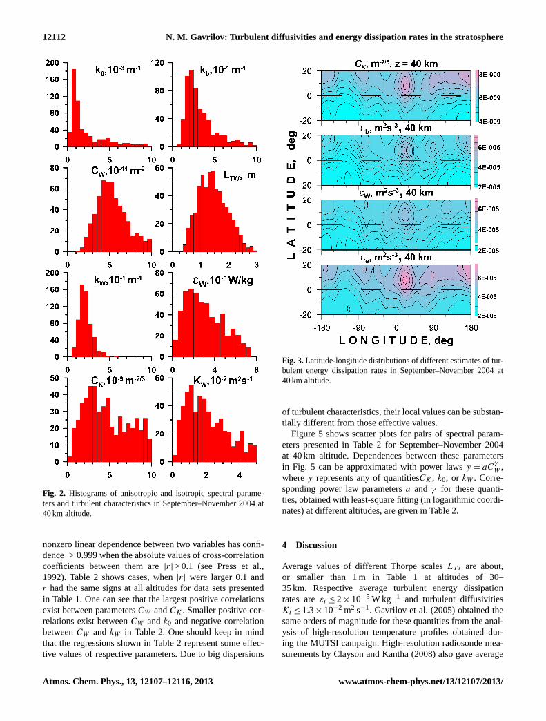
Because of the large spatial and temporal variability ofthe turbulent parameters, their statistical distributions couldbe more informative than just averages and standard disper-sions. Figure 2 presents histograms of the spectral parame-ters and turbulence characteristics for September–November2004 at 40 km altitude. Respective histograms for otherheights layers have forms similar to Fig. 2, and their pa-rameters are given in Table 1. All histograms in Fig. 2 havestrongly non-Gaussian shapes.

For January 2005 Table 1 gives estimations of the av-erage Thorpe scales by different approaches in the rangeLT ∼ 0.34–0.44 m at 30 km altitude at latitudes 34–36◦ N.Respective average turbulent energy dissipation rates in Ta-ble 1 areε ∼ (1.8–2.9)× 10−6 W kg−1 and turbulent diffu-sivities K ∼ (1.3–2.0)× 10−3 m2s−1. Dispersions in theseestimations are caused by usage of differentkm = kb andkm = kW in Eq. (12) for calculation ofLT b and LT W andusage of Eq. (13) to calculateLT e, also by possible uncer-tainties in semi-empirical coefficients in these formulae.



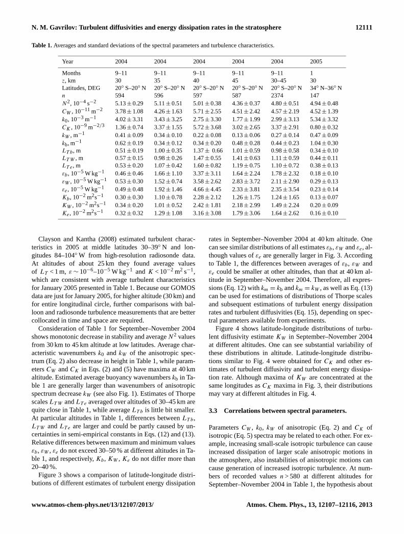
Table 1.Averages and standard deviations of the spectral parameters and turbulence characteristics.

Year 2004 2004 2004 2004 2004 2005

Months 9–11 9–11 9–11 9–11 9–11 1z, km 30 35 40 45 30–45 30Latitudes, DEG 20◦ S–20◦ N 20◦ S–20◦ N 20◦ S–20◦ N 20◦ S–20◦ N 20◦ S–20◦ N 34◦ N–36◦ Nn 594 596 597 587 2374 147N2, 10−4 s−2 5.13± 0.29 5.11± 0.51 5.01± 0.38 4.36± 0.37 4.80± 0.51 4.94± 0.48CW , 10−11m−2 3.78± 1.08 4.26± 1.63 5.71± 2.55 4.51± 2.42 4.57± 2.19 4.52± 1.39k0, 10−3 m−1 4.02± 3.31 3.43± 3.25 2.75± 3.30 1.77± 1.99 2.99± 3.13 5.34± 3.32CK , 10−9 m−2/3 1.36± 0.74 3.37± 1.55 5.72± 3.68 3.02± 2.65 3.37± 2.91 0.80± 0.32kW , m−1 0.41± 0.09 0.34± 0.10 0.22± 0.08 0.13± 0.06 0.27± 0.14 0.47± 0.09kb, m−1 0.62± 0.19 0.34± 0.12 0.34± 0.20 0.48± 0.28 0.44± 0.23 1.04± 0.30LT b, m 0.51± 0.19 1.00± 0.35 1.37± 0.66 1.01± 0.59 0.98± 0.58 0.34± 0.10LT W , m 0.57± 0.15 0.98± 0.26 1.47± 0.55 1.41± 0.63 1.11± 0.59 0.44± 0.11LT e, m 0.53± 0.20 1.07± 0.42 1.60± 0.82 1.19± 0.75 1.10± 0.72 0.38± 0.13εb, 10−5 W kg−1 0.46± 0.46 1.66± 1.10 3.37± 3.11 1.64± 2.24 1.78± 2.32 0.18± 0.10εW , 10−5 W kg−1 0.53± 0.30 1.52± 0.74 3.58± 2.62 2.83± 3.72 2.11± 2.90 0.29± 0.13εe, 10−5 W kg−1 0.49± 0.48 1.92± 1.46 4.66± 4.45 2.33± 3.81 2.35± 3.54 0.23± 0.14Kb, 10−2 m2s−1 0.30± 0.30 1.10± 0.78 2.28± 2.12 1.26± 1.75 1.24± 1.65 0.13± 0.07KW , 10−2 m2s−1 0.34± 0.20 1.01± 0.52 2.42± 1.81 2.18± 2.99 1.49± 2.24 0.20± 0.09Ke, 10−2 m2s−1 0.32± 0.32 1.29± 1.08 3.16± 3.08 1.79± 3.06 1.64± 2.62 0.16± 0.10

Clayson and Kantha (2008) estimated turbulent charac-teristics in 2005 at middle latitudes 30–39◦ N and lon-gitudes 84–104◦ W from high-resolution radiosonde data.At altitudes of about 25 km they found average valuesof LT < 1 m, ε ∼ 10−6–10−5 W kg−1 and K < 10−2 m2 s−1,which are consistent with average turbulent characteristicsfor January 2005 presented in Table 1. Because our GOMOSdata are just for January 2005, for higher altitude (30 km) andfor entire longitudinal circle, further comparisons with bal-loon and radiosonde turbulence measurements that are bettercollocated in time and space are required.

Consideration of Table 1 for September–November 2004shows monotonic decrease in stability and averageN2 valuesfrom 30 km to 45 km altitude at low latitudes. Average char-acteristic wavenumbersk0 andkW of the anisotropic spec-trum (Eq. 2) also decrease in height in Table 1, while param-etersCW andCK in Eqs. (2) and (5) have maxima at 40 kmaltitude. Estimated average buoyancy wavenumberskb in Ta-ble 1 are generally larger than wavenumbers of anisotropicspectrum decreasekW (see also Fig. 1). Estimates of ThorpescalesLT W andLT e averaged over altitudes of 30–45 km arequite close in Table 1, while averageLT b is little bit smaller.At particular altitudes in Table 1, differences betweenLT b,LT W andLT e are larger and could be partly caused by un-certainties in semi-empirical constants in Eqs. (12) and (13).Relative differences between maximum and minimum valuesεb, εW , εe do not exceed 30–50 % at different altitudes in Ta-ble 1, and respectively,Kb, KW , Ke do not differ more than20–40 %.

Figure 3 shows a comparison of latitude-longitude distri-butions of different estimates of turbulent energy dissipation

rates in September–November 2004 at 40 km altitude. Onecan see similar distributions of all estimatesεb, εW andεe, al-though values ofεe are generally larger in Fig. 3. Accordingto Table 1, the differences between averages ofεb, εW andεe could be smaller at other altitudes, than that at 40 km al-titude in September–November 2004. Therefore, all expres-sions (Eq. 12) withkm = kb andkm = kW , as well as Eq. (13)can be used for estimations of distributions of Thorpe scalesand subsequent estimations of turbulent energy dissipationrates and turbulent diffusivities (Eq. 15), depending on spec-tral parameters available from experiments.

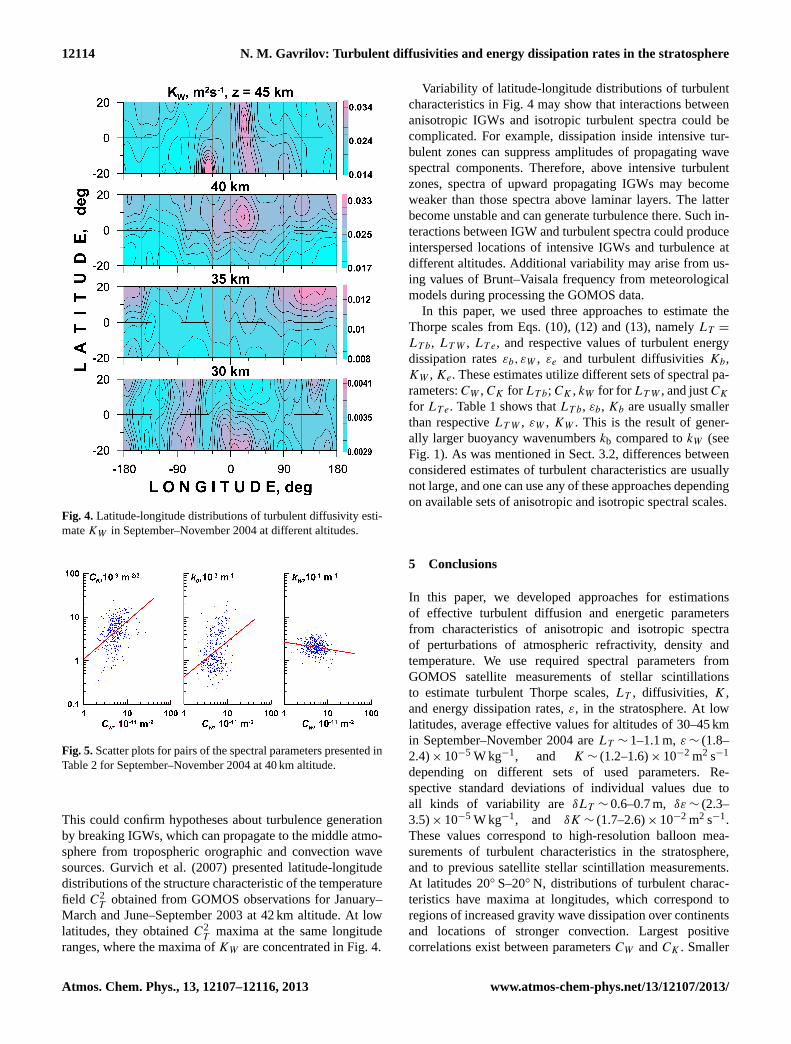
Figure 4 shows latitude-longitude distributions of turbu-lent diffusivity estimateKW in September–November 2004at different altitudes. One can see substantial variability ofthese distributions in altitude. Latitude-longitude distribu-tions similar to Fig. 4 were obtained forCK and other es-timates of turbulent diffusivity and turbulent energy dissipa-tion rate. Although maxima ofKW are concentrated at thesame longitudes asCK maxima in Fig. 3, their distributionsmay vary at different altitudes in Fig. 4.

3.3 Correlations between spectral parameters.

ParametersCW , k0, kW of anisotropic (Eq. 2) andCK ofisotropic (Eq. 5) spectra may be related to each other. For ex-ample, increasing small-scale isotropic turbulence can causeincreased dissipation of larger scale anisotropic motions inthe atmosphere, also instabilities of anisotropic motions cancause generation of increased isotropic turbulence. At num-bers of recorded valuesn > 580 at different altitudes forSeptember–November 2004 in Table 1, the hypothesis about



Fig. 2. Histograms of anisotropic and isotropic spectral parame-ters and turbulent characteristics in September–November 2004 at40 km altitude.

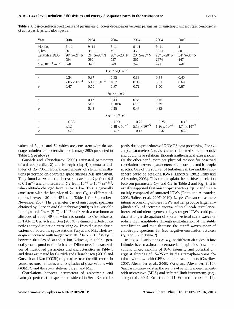
nonzero linear dependence between two variables has confi-dence> 0.999 when the absolute values of cross-correlationcoefficients between them are|r| > 0.1 (see Press et al.,1992). Table 2 shows cases, when|r| were larger 0.1 andr had the same signs at all altitudes for data sets presentedin Table 1. One can see that the largest positive correlationsexist between parametersCW andCK . Smaller positive cor-relations exist betweenCW andk0 and negative correlationbetweenCW andkW in Table 2. One should keep in mindthat the regressions shown in Table 2 represent some effec-tive values of respective parameters. Due to big dispersions

Fig. 3.Latitude-longitude distributions of different estimates of tur-bulent energy dissipation rates in September–November 2004 at40 km altitude.

of turbulent characteristics, their local values can be substan-tially different from those effective values.

Figure 5 shows scatter plots for pairs of spectral param-eters presented in Table 2 for September–November 2004at 40 km altitude. Dependences between these parametersin Fig. 5 can be approximated with power lawsy = aC

γ

W ,wherey represents any of quantitiesCK , k0, or kW . Corre-sponding power law parametersa and γ for these quanti-ties, obtained with least-square fitting (in logarithmic coordi-nates) at different altitudes, are given in Table 2.

4 Discussion

Average values of different Thorpe scalesLT i are about,or smaller than 1 m in Table 1 at altitudes of 30–35 km. Respective average turbulent energy dissipationrates areεi ≤ 2× 10−5 W kg−1 and turbulent diffusivitiesKi ≤ 1.3× 10−2 m2 s−1. Gavrilov et al. (2005) obtained thesame orders of magnitude for these quantities from the anal-ysis of high-resolution temperature profiles obtained dur-ing the MUTSI campaign. High-resolution radiosonde mea-surements by Clayson and Kantha (2008) also gave average



Table 2. Cross-correlation coefficients and parameters of power dependences between parameters of anisotropic and isotropic componentsof atmospheric perturbation spectra.

Year 2004 2004 2004 2004 2004 2005

Months 9–11 9–11 9–11 9–11 9–11 1z, km 30 35 40 45 30–45 30Latitudes, DEG 20◦ S–20◦ N 20◦ S–20◦ N 20◦ S–20◦ N 20◦ S–20◦ N 20◦ S–20◦ N 34◦ S–36◦ Nn 594 596 597 587 2374 147CW ,10−11m−2 3–8 3–8 2–9 2–9 2–11 2–8

CK ∼ a(CW )γ

r 0.24 0.37 0.32 0.36 0.44 0.49a 2.05× 10−4 5.17× 10−4 48.7 0.068 55.1 0.69γ 0.47 0.50 0.97 0.72 1.00 0.87

k0 ∼ a(CW )γ

r 0.13 0.33 0.38 0.15a 50.0 1.10E6 61.6 0.39γ 0.42 0.85 0.45 0.22

kW ∼ a(CW )γ

r −0.36 −0.20 −0.20 −0.25 −0.45a 8.12 7.48× 10−3 5.18× 10−3 1.26× 10−4 1.74× 10−3

γ −0.35 −0.14 −0.13 −0.32 −0.23

values ofLT , ε, andK, which are consistent with the av-erage turbulent characteristics for January 2005 presented inTable 1 (see above).

Gurvich and Chunchuzov (2003) estimated parametersof anisotropic (Eq. 2) and isotropic (Eq. 4) spectra at alti-tudes of 25–70 km from measurements of stellar scintilla-tions performed on-board the space stations Mir and Salyut.They found a systematic decrease in averagekW from 0.5to 0.1 m−1 and an increase inCK from 10−9 to 10−8 m−2/3,when altitude changed from 30 to 50 km. This is generallyconsistent with the behavior ofkW andCK at different al-titudes between 30 and 45 km in Table 1 for September–November 2004. The parameterCW of anisotropic spectrumobtained by Gurvich and Chunchuzov (2003) is less variablein height andCW ∼ (5–7)× 10−11 m−2 with a maximum ataltitudes of about 40 km, which is similar toCW behaviorin Table 1. Gurvich and Kan (2003b) estimated turbulent ki-netic energy dissipation rates usingkW from the same obser-vations on-board the space stations Salyut and Mir. Their av-erageε increased with height from 10−6 to 5× 10−5 W kg−1

between altitudes of 30 and 50 km. Valuesεi in Table 1 gen-erally correspond to this behavior. Differences in exact val-ues of mentioned parameters and characteristics in Table 1and those estimated by Gurvich and Chunchuzov (2003) andGurvich and Kan (2003b) might arise from the differences inyears, seasons, latitudes and longitudes of observations withGOMOS and the space stations Salyut and Mir.

Correlations between parameters of anisotropic andisotropic perturbation spectra considered in Sect. 3.3 can be

partly due to procedures of GOMOS data processing. For ex-ample, parametersCW , k0, kW are calculated simultaneouslyand could have relations through mathematical expressions.On the other hand, there are physical reasons for observedcorrelations between parameters of anisotropic and isotropicspectra. One of the sources of turbulence in the middle atmo-sphere could be breaking IGWs (Lindzen, 1981; Fritts andAlexander, 2003). This could explain the positive correlationbetween parametersCW andCK in Table 2 and Fig. 5. It isusually supposed that anisotropic spectra (Eqs. 2 and 3) aremainly composed of saturated IGWs (Fritts and Alexander,2003; Sofieva et al., 2007, 2010). LargerCW can cause moreintensive breaking of these IGWs and can produce larger am-plitudesCK of isotropic spectra of small-scale turbulence.Increased turbulence generated by stronger IGWs could pro-duce stronger dissipation of shorter vertical scale waves orreduce their amplitudes through neutralization of the stablestratification and thus decrease the cutoff wavenumber ofanisotropic spectrumkW (see negative correlation betweenCW andkW in Table 2).

In Fig. 4, distributions ofKW at different altitudes in lowlatitudes have maxima concentrated at longitudes close to lo-cations where maxima of IGW intensity and potential en-ergy at altitudes of 15–25 km in the stratosphere were ob-tained with low-orbit GPS satellite measurements (Gavrilov,2007; Alexander et al., 2008; Wang and Alexander, 2010).Similar maxima exist in the results of satellite measurementswith microwave (MLS) and infrared limb instruments (e.g.,Jiang et al., 2004; Ern et al., 2011; Ern and Preusse, 2012).



Fig. 4. Latitude-longitude distributions of turbulent diffusivity esti-mateKW in September–November 2004 at different altitudes.

Fig. 5.Scatter plots for pairs of the spectral parameters presented inTable 2 for September–November 2004 at 40 km altitude.

This could confirm hypotheses about turbulence generationby breaking IGWs, which can propagate to the middle atmo-sphere from tropospheric orographic and convection wavesources. Gurvich et al. (2007) presented latitude-longitudedistributions of the structure characteristic of the temperaturefield C2

T obtained from GOMOS observations for January–March and June–September 2003 at 42 km altitude. At lowlatitudes, they obtainedC2

T maxima at the same longituderanges, where the maxima ofKW are concentrated in Fig. 4.

Variability of latitude-longitude distributions of turbulentcharacteristics in Fig. 4 may show that interactions betweenanisotropic IGWs and isotropic turbulent spectra could becomplicated. For example, dissipation inside intensive tur-bulent zones can suppress amplitudes of propagating wavespectral components. Therefore, above intensive turbulentzones, spectra of upward propagating IGWs may becomeweaker than those spectra above laminar layers. The latterbecome unstable and can generate turbulence there. Such in-teractions between IGW and turbulent spectra could produceinterspersed locations of intensive IGWs and turbulence atdifferent altitudes. Additional variability may arise from us-ing values of Brunt–Vaisala frequency from meteorologicalmodels during processing the GOMOS data.

In this paper, we used three approaches to estimate theThorpe scales from Eqs. (10), (12) and (13), namelyLT =

LT b, LT W , LT e, and respective values of turbulent energydissipation ratesεb,εW , εe and turbulent diffusivitiesKb,KW , Ke. These estimates utilize different sets of spectral pa-rameters:CW , CK for LT b; CK , kW for for LT W , and justCK

for LT e. Table 1 shows thatLT b, εb, Kb are usually smallerthan respectiveLT W , εW , KW . This is the result of gener-ally larger buoyancy wavenumberskb compared tokW (seeFig. 1). As was mentioned in Sect. 3.2, differences betweenconsidered estimates of turbulent characteristics are usuallynot large, and one can use any of these approaches dependingon available sets of anisotropic and isotropic spectral scales.

5 Conclusions

In this paper, we developed approaches for estimationsof effective turbulent diffusion and energetic parametersfrom characteristics of anisotropic and isotropic spectraof perturbations of atmospheric refractivity, density andtemperature. We use required spectral parameters fromGOMOS satellite measurements of stellar scintillationsto estimate turbulent Thorpe scales,LT , diffusivities, K,and energy dissipation rates,ε, in the stratosphere. At lowlatitudes, average effective values for altitudes of 30–45 kmin September–November 2004 areLT ∼ 1–1.1 m,ε ∼ (1.8–2.4)× 10−5 W kg−1, and K ∼ (1.2–1.6)× 10−2 m2 s−1

depending on different sets of used parameters. Re-spective standard deviations of individual values due toall kinds of variability are δLT ∼ 0.6–0.7 m, δε ∼ (2.3–3.5)× 10−5 W kg−1, and δK ∼ (1.7–2.6)× 10−2 m2 s−1.These values correspond to high-resolution balloon mea-surements of turbulent characteristics in the stratosphere,and to previous satellite stellar scintillation measurements.At latitudes 20◦ S–20◦ N, distributions of turbulent charac-teristics have maxima at longitudes, which correspond toregions of increased gravity wave dissipation over continentsand locations of stronger convection. Largest positivecorrelations exist between parametersCW andCK . Smaller



positive correlations may exist betweenCW and k0, alsonegative correlation betweenCW andkW .

Acknowledgements.This work was partly supported by theRussian Basic Research Foundation. The author thanks Victoria F.Sofieva for providing databases of parameters of anisotropic andisotropic temperature perturbation spectra from GOMOS satellitemeasurements and for useful discussions.

Edited by: P. Haynes

References

Alexander, M. J., Tsuda, T., and Vincent, R. A.: Latitudinal varia-tions observed in gravity waves with short vertical wavelengths,J. Atmos. Sci., 59, 1394–1404, 2002.

Alexander, M. J., Geller, M., McLandress, C., Polavarapu, S.,Preusse, P., Sassi, F., Sato, K., Eckermann, S., Ern, M., Hertzog,A., Kawatani, Y. A., Pulido, M., Shaw, T., Sigmond, M., Vin-cent, R., and Watanabe, S.: Recent developments in gravity-waveeffects in climate models and the global distribution of gravity-wave momentum flux from observations and models, Q. J. Roy.Meteorol. Soc. 136, 1103–1124, doi:10.1002/qj.637, 2010.

Alexander, S. P., Tsuda, T., Kawatani, Y., and Takahashi, M.:Global distribution of atmospheric waves in the equatorial up-per troposphere and lower stratosphere: COSMIC observationsof wave mean flow interactions, J. Geophys. Res., 113, D24115,doi:10.1029/2008JD010039, 2008.

Alisse, J. R.: Turbulence en atmosphere stable, Une etude quantita-tive, These de doctorat, Univ. Paris VI, 1999.

Bertaux, J. L., Kyrola, E., Fussen, D., Hauchecorne, A., Dalaudier,F., Sofieva, V., Tamminen, J., Vanhellemont, F., Fanton d’Andon,O., Barrot, G., Mangin, A., Blanot, L., Lebrun, J. C., Perot, K.,Fehr, T., Saavedra, L., Leppelmeier, G. W., Fraisse, R.: Globalozone monitoring by occultation of stars: an overview of GO-MOS measurements on ENVISAT, Atmos. Chem. Phys., 10,12091–12148, doi:10.5194/acp-10-12091-2010, 2010.

Caldwell, D. R.: Oceanic turbulence: big bangs or continuous cre-ation?, J. Geophys. Res., 88, 7543–7550, 1983.

Clayson, C. A., Kantha, L.: On turbulence and mixing in the freeatmosphere inferred from high-resolution soundings, J. Atmos.Ocean. Technol., 25, 833–851, 2008.

Eckermann, S. and Preusse, P.: Global measurements of strato-spheric mountain waves from space, Science, 286, 1534-1537,1999.

Ern, M. and Preusse, P.: Gravity wave momentum flux spectraobserved from satellite in the summertime subtropics: Implica-tions for global modeling, Geophys. Res. Letters, 39, L15810,doi:10.1029/2012GL052659, 2012.

Ern, M., Preusse, P., Alexander, M. J., and Warner, C.D.: Absolute values of gravity wave momentum flux de-rived from satellite data, J. Geophys. Res., 109, D20103,doi:10.1029/2004JD004752, 2004.

Ern, M., Preusse, P., Gille, J. C., Hepplewhite, C. L., Mlynczak, M.G., Russell III, J. M., and Riese M.: Implications for atmosphericdynamics derived from global observations of gravity wave mo-mentum flux in stratosphere and mesosphere, J. Geophys. Res.,116, D19107, doi:10.1029/2011JD015821, 2011.

Fer, I., Skogseth, R., and Haugan, P. M.: Mixing of the Storjor-den overflow (Svalbard Archipelago) inferred from density over-turns, J. Geophys. Res., 109, 1–14, 2004.

Fetzer, E. J. and Gille, J. C.: Gravity wave variance in LIMS tem-peratures. Part I: Variability and comparison with backgroundwinds, J. Atmos. Sci., 51, 2461–2483, 1994.

Fritts, D. C. and Alexander, M. J.: Gravity wave dynamics andeffects in the middle atmosphere, Rev. Geophys. 41, 1003,doi:10.1029/2001RG000106, 2003.

Fukao, S., Yamanaka, M. D., Ao, N., Hocking, W. K., Sato, T., Ya-mamoto, M., Nakamura, T., Tsuda, T., and Kato, S.: Seasonalvariability of vertical eddy diffusivity in the middle atmosphere,1. Three-year observations by the middle and upper atmosphereradar, J. Geophys. Res., 99, 18973–18987, 1994.

Galbraith, P. S. and Kelley, D. E.: Identifying overturns in CTD pro-files, J. Atmos. Ocean. Technol., 13, 688–702, 1996.

Gavrilov, N. M.: Structure of the mesoscale variability of the tro-posphere and stratosphere found from radio refraction measure-ments via CHAMP satellite, Izvestiya, Atmos. Ocean. Phys., 43,451–460, 2007.

Gavrilov, N. M. and Karpova, N. V.: Global structure of mesoscalevariability of the atmosphere from satellite measurements of ra-dio wave refraction, Izvestia, Atmos. Ocean. Phys., 40, 747–758,2004.

Gavrilov, N. M., Karpova, N. V., Jacobi, Ch., and Gavrilov, A. N.:Morphology of atmospheric refraction index variations at dif-ferent altitudes from GPS/MET satellite observations, J. Atmos.Sol.-Terr. Phys., 66, 427–435, 2004.

Gavrilov, N. M., Luce, H., Crochet, M., Dalaudier, F., and Fukao,S.: Turbulence parameter estimations from high-resolution bal-loon temperature measurements of the MUTSI-2000 campaign,Ann. Geophys., 23, 2401–2413, doi:10.5194/angeo-23-2401-2005, 2005.

Gurvich, A. S. and Brekhovskikh, V. L.: Study of the turbulenceand inner waves in the stratosphere based on the observations ofstellar scintillations from space: A model of scintillation spectra,Waves Random Media, 11, 163–181, 2001.

Gurvich, A. S. and Chunchuzov, I. P.: Parameters of the fine den-sity structure in the stratosphere obtained from spacecraft ob-servations of stellar scintillations, J. Geophys. Res., 108, 4166,doi:10.1029/2002JD002281, 2003.

Gurvich, A. S. and Kan V.: Structure of air density irregularities inthe stratosphere from spacecraft observations of stellar scintilla-tion: 1. Three-dimensional spectrum model and recovery of itsparameters, Izvestia, Atmos. Ocean. Phys., 39, 300–310, 2003a.

Gurvich, A. S. and Kan V.: Structure of air density irregularities inthe stratosphere from spacecraft observations of stellar scintilla-tion: 2. Characteristic scales, structure characteristics, and kineticenergy dissipation, Izvestiya, Atmos. Ocean. Phys., 39, 311–321,2003b.

Gurvich, A. S., Kan, V., Savchenko, S. A., Pakhomov, A. I.,Padalka, G. I.: Studying the turbulence and internal waves in thestratosphere from spacecraft observations of stellar scintillation:II. Probability distributions and scintillation spectra, Izvestia, At-mos. Ocean. Phys., 37, 452–465, 2001.

Gurvich, A. S., Sofieva, V. F., and Dalaudier, F.: Global distribu-tion of CT 2 at altitudes 30–50 km from space-borne observa-tions of stellar scintillation. Geophys. Res. Lett., 34, L24813,doi:10.1029/2007GL031134, 2007.


http://dx.doi.org/10.1002/qj.637

http://dx.doi.org/10.1029/2008JD010039

http://dx.doi.org/10.5194/acp-10-12091-2010

http://dx.doi.org/10.1029/2012GL052659

http://dx.doi.org/10.1029/2004JD004752

http://dx.doi.org/10.1029/2011JD015821

http://dx.doi.org/10.1029/2001RG000106

http://dx.doi.org/10.5194/angeo-23-2401-2005

http://dx.doi.org/10.5194/angeo-23-2401-2005

http://dx.doi.org/10.1029/2002JD002281

http://dx.doi.org/10.1029/2007GL031134


Jiang, J. H., Wang, B., Goya, K., Hocke, K., Eckermann, S. D.,Ma, J., Wu, D. L., and Read, W. J.: Geographical distributionand interseasonal variability of tropical deep convection: UARSMLS observations and analyses, J. Geophys. Res., 109, D03111,doi:10.1029/2003JD003756, 2004.

Lindzen, R. S.: Turbulence and Stress Owing to Gravity Wave andTidal Breakdown, J. Geophys. Res., 86, 9707–9714, 1981.

Lumley, J. L.: The spectrum of nearly inertial turbulence in a stablystratified fluid, J. Atmos. Sci., 21, 99–102, 1964.

McLandress, C., Alexander, M. J., and Wu, D.: Microwave limbsounder observations of gravity waves in the stratosphere: Aclimatology and interpretation, J. Geophys. Res., 105, 11947–11967, 2000.

Monin, A. S. and Yaglom, A. M.: Statistical Fluid Mechanics, vol.2, MIT Press, Cambridge, Mass., 1975.

Ottersten H.: Atmospheric structure and radar backscattering inclear air, Radio Sci., 4, 1179–1193, 1969.

Press, W. H., Teukolsky, S. A., Vetterling, W. T., Flannery, B. P.: Nu-merical Recipes in FORTRAN, The Art of Scientific Computing,Oxford, Clarendon, 1992.

Schmidt, T., de la Torre, A., and Wickert, J.: Global grav-ity wave activity in the tropopause region from CHAMPradio occultation data, Geophys. Res. Lett., 35, L16807,doi:10.1029/2008GL034986, 2008.

Smith, S. A., Fritts, D. C., and VanZandt, T. E.: Evidence of a satu-ration spectrum of atmospheric gravity waves, J. Atmos. Sci., 44,1404–1410, 1987.

Sofieva, V. F., Gurvich, A. S., Dalaudier, F., and Kan, V.: Recon-struction of internal gravity wave and turbulence parameters inthe stratosphere using GOMOS scintillation measurements, J.Geophys. Res., 112, D12113, doi:10.1029/2006JD007483, 2007.

Sofieva, V. F., Gurvich, A. S., and Dalaudier, F.: Gravity wavespectra parameters in 2003 retrieved from stellar scintillationmeasurements by GOMOS, Geophys. Res. Lett., 36, L05811,doi:10.1029/2008GL036726, 2009.

Sofieva, V. F., Gurvich, A. S., and Dalaudier, F.: Mapping grav-ity waves and turbulence in the stratosphere using satellite mea-surements of stellar scintillation, Physica Scripta, T142, 014043,doi:10.1088/0031-8949/2010/T142/014043, 2010.

Tatarskii, V. I.: The Effects of the Turbulent Atmosphere on WavePropagation, US Dep. of Commer., Washington, DC, 1971.

Tsuda, T., Nishida, M., Rocken, C., and Ware, R. H.: A global mor-phology of gravity wave activity in the stratosphere revealed bythe GPS occultation data (GPS/MET), J. Geophys. Res., 105,7257–7274, 2000.

Wang, L. and Alexander, M. J.: Global estimates of gravity waveparameters from GPS radio occultation temperature data, J. Geo-phys. Res., 115, D21122, doi:10.1029/2010JD013860, 2010.

Wu, D. and Waters, J.: Gravity-wave-scale temperature fluctuationsseen by the UARS MLS, Geophys. Res. Lett., 23, 3289–3292,1996.

Wu, D. L., Preusse, P., Eckermann, S. D., Jiang, J. H., de la Torre,J. M., Coy, L., Lawrence, B., and Wang, D. Y.: Remote sound-ing of atmospheric gravity waves with satellite limb and nadirtechniques, Adv. Space Res., 37, 2269–2277, 2006.


http://dx.doi.org/10.1029/2003JD003756

http://dx.doi.org/10.1029/2008GL034986

http://dx.doi.org/10.1029/2006JD007483

http://dx.doi.org/10.1029/2008GL036726

http://dx.doi.org/10.1088/0031-8949/2010/T142/014043

http://dx.doi.org/10.1029/2010JD013860

estimates of turbulent diffusivities and energy dissipation rates from

Documents