estimates of sea surface height and near-surface...

Estimates of sea surface height and near-surface alongshore coastal

currents from combinations of altimeters and tide gauges

M. Saraceno,1,2 P. T. Strub,1 and P. M. Kosro1

Received 31 January 2008; revised 8 August 2008; accepted 25 August 2008; published 15 November 2008.

[1] Present methods used to retrieve altimeter data do not provide reliable estimates ofsea surface height (SSH) in the nearshore region, resulting in a measurement gap of25–50 km next to the coast. In the present work, gridded SSH fields produced byArchiving, Validation, and Interpretation of Satellite Oceanographic data (AVISO) in theoffshore region are combined with coastal tide gauge time series of SSH to improveestimation in that gap along the west coast of the United States in the northern CaliforniaCurrent System between 40� and 45�N and 123.8� and 126�W. To assess the increasein skill provided by this procedure, the geostrophic alongshore currents, calculated fromthe new SSH fields in the gap region, are compared to three in situ, nearshore currentmeasurements, resulting in correlation coefficients of 0.73–0.83 and standard deviationsof the differences of 11.6–12.6 cm/s, substantially improved from the AVISO-only results.When the Ekman current components are estimated and added to the geostrophiccurrents, comparisons to the 10 m deep acoustic Doppler current profiler velocities areonly slightly improved. The Ekman components make a more significant contributionwhen compared to HF radar surface current measurements, providing correlations of0.94 and standard deviations of the differences of 6.4–9.5 cm/s. These results represent adramatic improvement in the quality of the SSH fields and estimated alongshorecurrents when additional, realistic SSH data from the coastal region are added.Here we use coastal tide gauges to provide the additional SSH data but also discuss moregeneral approaches for altimeter SSH retrievals in coastal regions where tidegauge data are not available.

Citation: Saraceno, M., P. T. Strub, and P. M. Kosro (2008), Estimates of sea surface height and near-surface alongshore coastal

currents from combinations of altimeters and tide gauges, J. Geophys. Res., 113, C11013, doi:10.1029/2008JC004756.

1. Introduction

[2] Satellite altimetry provides a unique opportunity tounderstand the dynamics of the sea, with sea surface height(SSH) data extending over the past 15 or more years. Theusefulness of the altimeter measurements for large-scalestudies is well established, as demonstrated by studies of thelarge-scale California Current on seasonal and interannualtimescales [Kelly et al., 1998; Strub and James, 2000,2002a, 2002b]. However, coastal processes are more diffi-cult to resolve with altimeter data, because of two types ofproblems. First, and most importantly, intrinsic difficultiesaffect the corrections applied to the altimeter data near thecoast (e.g., the wet tropospheric component, high-frequencyoceanographic signals, tidal corrections, etc.). Thus, data areusually flagged as unreliable within some distance of thecoast. Second, the interpolation of along-track data collectedby just one or two satellites provides only marginal resolu-

tion of mesoscale and smaller-scale structure in oceancirculation [Le Traon and Dibarboure, 2002; Leeuwenburghand Stammer, 2002; Chelton and Schlax, 2003], which isdominant in the coastal region.[3] Several approaches are available to address the prob-

lems described above. Pascual et al. [2006, 2007] show thatincreasing the number of satellites used to produce griddedmaps of sea surface height to four greatly increases theaccuracy of estimates of the mesoscale surface circulation.Volkov et al. [2007] show that improvements in tidal andhigh-frequency models used to produce the data distributedby the Archiving, Validation, and Interpretation of SatelliteOceanographic data (AVISO) project also improve thequality of the altimeter SSH fields over wide continentalshelves. Other efforts to correct the altimeter signal near thecoast include recomputing the wet tropospheric correction[Manzella et al., 1997; Vignudelli et al., 2005; Madsen etal., 2007; Desportes et al., 2007], the use of customizedtidal modeling [Vignudelli et al., 2000; Volkov et al., 2007],the use of higher-rate data [Lillibridge, 2005], and/orretracking [Deng and Featherstone, 2006].[4] In the present work we address the first set of

problems described above by first estimating the distancefrom the coast within which the original along-track altim-

JOURNAL OF GEOPHYSICAL RESEARCH, VOL. 113, C11013, doi:10.1029/2008JC004756, 2008ClickHere

for

FullArticle

1College of Oceanic and Atmospheric Sciences, Oregon StateUniversity, Corvallis, Oregon, USA.

2Currently at Centro de Investigaciones del Mar y la Atmosfera, CiudadUniversitaria, Buenos Aires, Argentina.

Copyright 2008 by the American Geophysical Union.0148-0227/08/2008JC004756$09.00

C11013 1 of 20

http://dx.doi.org/10.1029/2008JC004756

eter data are usually (>75% of the time) flagged as unreli-able. Because of the lack of valid data, gridded AVISOaltimeter fields in this coastal ‘‘gap’’ region are mostly theresult of the extrapolation of nearby offshore data. However,as we shall show, this procedure is often unreliable. Aftereliminating the AVISO data in this gap, we produce newSSH fields by interpolating between the tide gauge SSH dataset along the coast and the gridded SSH data set produced byAVISO in the offshore region. To assess the improvementresulting from this simple approach, alongshore geostrophiccurrents, estimated from the new SSH fields, are thencompared to in situ acoustic Doppler current profiler(ADCP) currents and surface current measurements fromCODAR SeaSonde HF mapping systems (‘‘HF currents’’)within the gap and the statistics of the comparisons arepresented.[5] The domain considered in this work is the northern

California Current System (CCS) between 40� and 45�Nand 123.8� and 126�W. In most of this region, the conti-nental shelf is relatively narrow and deep, reducing theeffects of tidal model errors in the altimeter data set. Thisportion of the coastal ocean off Oregon has been the focusof a number of in situ process studies, beginning with theWisp and Coastal Upwelling Experiments (CUE-I andCUE-II) in the early 1970s, continuing through theGLOBEC (Global Ocean Ecosystem Experiment) andCOAST (Coastal Ocean Advances in Shelf Transport)projects during 1997–2003. The early studies resulted intwo-dimensional (onshore-offshore) conceptual models ofupwelling systems [Kundu et al., 1975; Kundu and Allen,1976; Huyer et al., 1978, 1979]. The in situ currentmeasurements, surveys and satellite data starting in 1997revealed greater three-dimensional complexity in the meso-scale circulation fields [Barth et al., 2000, 2005a, 2005b;Kosro, 2005]. The results of studies through the early 1990sare included in reviews of the CCS physical oceanographyby [Hickey, 1979, 1998]. Mackas et al. [2006] include thelater studies and extend the scope of the review to includebiological responses to the physical forcing, upwelling andmesoscale circulation patterns.[6] In the northern CCS, wind stress, coastal SSH and

strong coastal currents reverse seasonally [Hickey, 1979;Strub et al., 1987; Hickey, 1998; Strub and James, 2000;Huyer et al., 2007]. In spring and summer, persistentequatorward winds (associated with the North Pacific High)produce upwelling, low sea levels next to the coast and anequatorward flowing jet that is found over or offshore of theshelf. In fall and winter, poleward winds (associated withsynoptic storms) produce downwelling, high sea levels nextto the coast and a poleward coastal jet, sometimes called theDavidson Current. In addition to forcing by the local orregional wind stress, buoyancy forcing by freshwater dis-charge at the coast influences the coastal circulation in somelocations, especially near the Columbia River Plume[Hickey, 1998; Huyer et al., 2005]. Winds located fartherto the south (off northern California) are also important,communicating their influence to the coastal ocean offcentral Oregon through the passage of poleward propagat-ing coastal trapped waves (CTW) [Allen, 1975; Smith, 1978;Brink, 1991; Hickey et al., 2006].[7] Tide gauges are commonly used to calibrate and

validate altimeter data [Leuliette et al., 2004], making them

a natural choice to extend altimeter SSH data to the coast. Inan early use of combinations of tide gauge and altimeterSSH data Strub and James [1997] demonstrated that theinclusion of tide gauge data allowed the SSH fields to showthe early development of an equatorward jet over the narrowshelf off central California in spring. The jet became visiblein the altimeter-only fields when it moved farther offshore.Off Oregon, the jet stays over the shelf and closer to thecoast for much of the spring and early summer [Kosro,2005], making it less visible to the altimeter-only SSHfields.[8] In the region studied here, five tide gauges are

distributed approximately evenly in latitude, providinglong-term SSH measurements. In addition, three in situmoorings with ADCPs [Kosro, 2003; Geier et al., 2006]and an array of HF surface current radars along the coast[Kosro, 2006] provide long-term current measurements forpart of the altimeter period that can be used to validate theincreased skill in geostrophic alongshore velocities estimat-ed from the new SSH fields in the coastal ‘‘gap.’’ Thepresence of strongly varying seasonal and synoptic currents,tide gauges, in situ current measurements and fairly simplecoastal geometry makes this an ideal location to test theability of combinations of altimeter and tide gauge data toresolve the alongshore coastal circulation.[9] This article is organized as follows: In section 2 we

present the satellite altimeter and tide gauge data, as well asthe in situ current meters and high-frequency surface currentmaps that are used to validate the results. In section 3, themethodology used to interpolate the data is explained andthe new gridded maps of SSH are compared to the mapsproduced by AVISO. Geostrophic velocities derived fromthe new SSH fields are compared to three time series of insitu current measurements and to the HF surface currentmaps in section 4, before and after adding Ekman compo-nents. A discussion of the results, their limitations andpossible future extensions concludes the article in section 5.

2. Data

2.1. Satellite Altimetry

[10] Two type of satellite altimeter data are used in thepresent work: along-track and gridded, both downloadedfrom the AVISO ftp site (data are available at ftp://ftp.cls.fr).We downloaded the along-track delayed time GeophysicalData Record (GDR) and the delayed time, updated version ofthe AVISO sea level anomaly weekly maps gridded at 1/4� inrectangular projection. The gridding technique for combiningmultisatellite data is described by Le Traon et al. [2003].AVISO gridded data are widely used to study the large-scaleandmesoscale currents, as well as to evaluate model SSH andsurface current fields (data are available at http://sealevel.jpl.nasa.gov). All data were corrected at AVISO, using standardtechniques for instrumental noise, orbit error, atmosphericattenuation (wet and dry tropospheric and ionosphericeffects), sea state bias, etc. A global adjustment using theTopex/Poseidon (T/P) orbit as a reference was performed toremove biases for all satellites [Le Traon and Ogor, 1998].Since 2005, all data have been retreated with a new tidalmodel (GOT2000) and a correction for the aliased high-frequency signals using a hydrodynamic model (MOG2D-G)[Carrere and Lyard, 2003]. The benefits in shallow waters of

C11013 SARACENO ET AL.: ESTIMATES OF COASTAL SEA SURFACE HEIGHT

2 of 20

C11013

those corrections compared to previous versions of the dataare discussed by Volkov et al. [2007]. Despite those correc-tions, along-track data show an important percentage ofmissing data as they approach the coast as quantified insection 3.2. However, the gridded AVISO fields do not have aconsistent gap near the coast, because of the extrapolation ofthe data to the coast (and over the coast, in some locations).

2.2. Tide Gauge Data

[11] Research quality hourly tide gauge (TG) data weredownloaded from the University of Hawaii Sea Level Center(data are available at http://ilikai.soest.hawaii.edu/uhslc) forthe same time period considered for the SSH: January 1993to December 2005. Data were retrieved from five stationsdistributed between 40�N and 45�N (Figure 1 and Table 1),with minimum and maximum distances between TGs of70 km and 144 km. There are gaps in the records at PortOrford (Oregon) and Crescent City (California); at the otherthree TGs, water level measurements were uninterrupted forthe period January 1993 to December 2005. These tidegauge records are from newer instruments and do not containthe type of errors described by Lentz [1993] and Harms andWinant [1994].

2.3. Independent Current Measurements

[12] In order to quantify the accuracy of the SSH pro-duced by merging TG and satellite data in the nearshoreregion, we correlated the geostrophic velocities derivedfrom the new SSH fields with three in situ time series ofvelocities estimated from upward looking acoustic Dopplercurrent profilers (ADCP) (see locations in Table 1) and HFsurface current maps. The moorings are part of the U.S.Global Ocean Ecosystem Dynamics (GLOBEC) program[Kosro, 2003; Geier et al., 2006]. HF surface current mapsare produced by the Ocean Currents Mapping Lab, OregonState University [Kosro, 2006] (data are available at http://bragg.coas.oregonstate.edu/) using an array of four long-range SeaSonde high-frequency surface current mappersdistributed along the Oregon coast, inside the region con-sidered. The methodology for these systems has beendescribed [Barrick et al., 1977; Lipa and Barrick, 1983].We used 1 year (2002) of low-pass filtered (46-h halfpower) gridded maps of HF surface currents.

2.4. Wind Data

[13] We used wind stress data to compute Ekman currentsat the locations corresponding to the position of the moor-

Figure 1. Along-track positions of Topex and Jason data.Empty (filled) circles indicate positions where more (less)than 75% of the data are present during the period January1993 to December 2005. The positions of the tide gaugesare indicated with filled squares.

Table 1. Location Name, Type of Instrument, Nearest Location at the Coast, Position, and Beginning and Ending Dates of the Time

Seriesa

Name of Location Instrument Latitude (�N) Longitude (�W)

Dates

Bin/Total Depth (m)Start End

Newport, Oregon ADCP 44.65 124.31 9 Aug 1997 31 Dec 2005 11/81Coos Bay, Oregon ADCP 43.16 124.57 22 Apr 2000 6 Sep 2004 10/100Rogue River, Oregon ADCP 42.44 124.57 9 Nov 2000 8 Sep 2004 10/69Crescent City, California TG 41.7 124.18 1 Jan 1993 31 Dec 2005Port Orford, Oregon TG 42.74 124.62 1 Jan 1993 31 Dec 2005Charleston, California TG 43.34 124.32 1 Jan 1993 31 Dec 2005South Beach, Oregon TG 44.63 124.04 1 Jan 1993 31 Dec 2005Humboldt Bay, California TG 40.77 124.22 1 Jan 1993 31 Dec 2005

aDepths of the velocity bin used and the total local depths are also indicated for the ADCPs. ADCP, acoustic Doppler current profiler; TG, tide gauge.


3 of 20

C11013

ings with the ADCP. Wind stress is computed from windspeed, which in the ocean is measured by in situ buoys or bythe satellite scatterometer QuikSCAT. To decide whichsource of data to use, we compared both. Wind data frombuoys were downloaded from the NOAA National DataBuoy Center website (www.ndbc.noaa.gov). The mooringlocated at Newport (South Beach) is very close (15.5 Km)to buoy 46050, which provides wind speed measurements.Unfortunately, this is not the case for the other two moor-ings: the nearest buoy (46015) provides measurements onlysince 21 July 2002, with a gap of nine months betweenOctober 2003 and July 2004. On the other hand, QuikSCATdata provide complete coverage of the surface of the oceansince 20 July 1999 to the present. We downloaded from theIfremer web site (data are available at www.ifremer.fr/cersat/) a gridded version of the QuikSCAT wind stress atdaily temporal resolution and 0.5� � 0.5� spatial resolution.Three time series were extracted at the locations nearest tothe moorings. The meridional component of the wind stress(which is the component that explains the highest percent-age of variance) as measured by QuikSCAT and by thebuoys are very similar (Table 2). Thus, we used the windstress estimated by the more complete QuikSCAT timeseries to compute the Ekman currents.

3. Methods

3.1. Preliminaries

3.1.1. Correlations[14] All the correlation coefficients cited are significant at

95% Confidence Level (CL), unless otherwise indicated.The significance levels of the scalar squared correlations areestimated from the c2 distribution on the basis of thenumber of independent observations (N*) estimated usingthe long lag method, following Davis [1976].3.1.2. TG Calibration[15] To suppress any tide-related signal, all TG data were

low-pass filtered with a 40-h (half power) Loess filter[Cleveland and Devlin, 1988]. Then, the inverse barometercorrection was applied using the 6-h reanalysis of Sea LevelPressure produced by the National Centers for Environmen-tal Prediction (NCEP).3.1.3. Low-Pass Filtering and SSH Calibration[16] The Nyquist frequency of the T/P and Jason data is

1/20 cycles per day. Thus a 20-day half-power Loess filterwas applied to the inverted barometer corrected TG timeseries. Current meter time series have also been low-passfiltered with the same 20-day low-pass Loess filter.[17] We estimate SSH anomalies by subtracting the time

average of the total record length at each point in the

altimeter SSH gridded maps and at the five TGs. This keepsall time-varying gradients of heights, the strongest of whichare associated with seasonal changes in alongshore jets,mesoscale meanders or eddies. Considering the relativesmall region used in the present work and that we areinterested in highlighting mesoscale structures, we prefernot to add uncertainties by adding a nonprecise meandynamic height (from climatology) to restore the largest-scale features. Mean dynamic heights in the region present aslight slope in the onshore-offshore direction, with lowervalues next to the coast [Strub and James, 2002a], consis-tent with weak (2–3 cm/s) equatorward flow. The analysisof temporal variability is not affected by the exclusion ofthis slope.

3.2. Estimation of the Gap

[18] Six satellite missions have collected SSH data duringour period of interest: Topex/Poseidon (T/P), ERS-1/2,Jason 1, Geosat Follow-On (GFO) and Envisat. Amongthose, T/P and Jason 1 shared the same tracks producing along record (23 September 1992 to present) at the highestfrequency (orbital repeat period is 9.916 days). Two of theT/P and Jason tracks that cover the region considered herepass very close to two of the tide gauges (Figure 1): theshortest distance between track 206 and the tide gauge atHumboldt Bay is 15.8 km; between track 69 and the tidegauge at Crescent City, it is 6.8 km. These two tracks areused to estimate the correlations between TGs and along-track SSH time series (Figure 2), which determine thedistance from the coast at which the satellite altimeterbecome routinely usable. For this purpose, a single timeseries from January 1993 to December 2005 is constructedfrom the T/P and Jason time series at each spatial locationof the along-track data. T/P flew between 23 September1992 and 25 August 2002 and Jason 1 has been flying since15 January 2000. Thus, before merging the data from thedifferent missions it is necessary to eliminate any differ-ences (biases) between T/P and Jason 1 SSH measurements.In order to do so, the following occurred:[19] 1. We added to the T/P time series the time mean of

the difference between it and the Jason 1 time series. Thedifference is estimated during the period when both satel-lites flew in the same orbits (15 January 2002 to 25 August2002).[20] 2. The temporal mean (estimated between January

1993 and December 2005) at each location is also removed.[21] More than 75% of the data available at each along-

track position are missing at distances shorter than 37 kmfrom the coast (Figures 1 and 2). This is due to intrinsicdifficulties in the corrections of the altimeter data (e.g., thewet tropospheric component, high-frequency oceanographicsignal, and tidal corrections) as well as issues related toland contamination in the footprint. At distances farther than37 km from the coast, less than 25% of the data are missing(Figure 1) and the correlation between the TG and thealong-track data decreases linearly with distance from thecoast (Figure 2). Thus we eliminated all of the gridded dataestimated by AVISO that fall within 37 km of the coast.

3.3. Creating a Denser TG Data Set Along the Coast

[22] The five time series of the filtered TGs are very wellcorrelated: among the 10 pairs of possible combinations, the

Table 2. Correlation Between the Meridional Wind Stress

Components as Estimated by QuikSCAT and Buoysa

Name of LocationLatitude(�N)

QuikSCAT Versus Buoys

Correlation(95% CL)

SD (Difference)(Pa)

Newport, Oregon 44.65 0.72 (0.16) 0.09Coos Bay, Oregon 43.16 0.75 (0.22) 0.12Rogue River, Oregon 42.44 0.79 (0.23) 0.14

aThe standard deviations (SD) of the differences between time series arealso shown. CL, Confidence Level.


4 of 20

C11013

minimum correlation is still very high (0.87, between SouthBeach, Oregon and Humboldt Bay, California, the mostwidely separated pair) indicating that at this scale, the signalretrieved by the TGs is quite uniform along the coast ontimescales of 20 days and longer. This result suggests that inthis region it is possible to create a denser spatial array ofvirtual tide gauges, uniformly distributed in latitude with nogaps in time. This is shown in Figure 3 (bottom), where theoriginal TGs have been interpolated into virtual TGs evenlydistributed along the coast, separated by 0.2� in latitude.The dense TG time series were also subsampled every 7 daysto match the exact SSH AVISO gridded dates.

3.4. Covering the Gap: Interpolation of TG WithSatellite Data

[23] To cover the gap next to the coast (i.e., the nearshoreregion indicated in Figures 4 (middle) and 5 (middle), thedense TG SSHs data set is interpolated to the AVISO griddedSSHs in the offshore region (i.e., west of the gap). Ourapproach here is to use a widely available method that isbased on the Delaunay triangulation method [Delaunay,1934]. The Delaunay triangulation technique consists ofbuilding a set of triangles by connecting all the data pointsin such a way that the vertices of the triangles are the datapoints. The collection of the edge’s triangles satisfies an‘‘empty circle’’ property: for each edge it is possible to find

a circle containing the edge’s endpoints but not containingany other data points. Figures 4 (middle) and 5 (middle)show the AVISO and TGs data sets (colored points), theregular grid (small black points) and the triangles selectedby the Delaunay triangulation (black lines). The value ateach grid point in the gap results from the weighted mean ofthe three data points located at the vertices of the trianglethat circumscribes the grid points considered, with weightsthat are inversely proportional to the distance between thegrid points and the data points. This technique is imple-mented by the ‘‘griddata’’ function in MATLAB, whichuses the Quickhull algorithm [Barber et al., 1996]. Theinterpolated time series produced by the ‘‘griddata’’ func-tion are not significantly different from results obtained byapplying an optimal interpolation method [Marcotte, 1991]to a limited representative number of fields. An advantageof using optimal interpolation methods is that they provideestimates of the errors. However, for the present application,error estimates are provided by the comparisons to in situdata.[24] In the next subsection we estimate the geostrophic

velocities associated with the new SSH fields. Because thegeostrophic velocities are proportional to the slope of theSSH, we applied a running median filter with a window sizeof 3 � 3 grid points to the individual SSH fields to avoidany discontinuities in the first derivative of the SSH fields at

Figure 2. Correlation coefficient (line with dots) and 95% CL (solid line) between time series of sealevel anomaly estimated from the TG at Humboldt Bay (California) and as measured by Topex and Jasonalong track 206, as a function of the distance from the coast. Vertical bars indicate the fraction of satellitedata missing at each position along track 206.


5 of 20

C11013

Figure

3.

(top)Tim

eseries

ofSSH

(m)as

measuredbythefivetidegauges.(bottom)Resultsoftheinterpolationofthe

fiveTGs’

timeseries

toadenseralongshore

grid(Figure

4).


6 of 20

C11013

their boundaries with the AVISO data along the edges ofthe gap region. Two examples of the result are shown inFigures 4 (right) and 5 (right).

3.5. Geostrophic Currents

[25] We estimate the geostrophic currents for each fieldthat resulted from merging TGs and satellite SSH. The zonaland meridional components of the geostrophic velocity at agiven grid point are estimated using centered difference as:

u x; yð Þ ¼ � g

f

� �� SSHx;yþ1 � SSHx;y�1

d x; yþ 1; y� 1ð Þ ð1Þ

v x; yð Þ ¼ g

f

� �� SSHxþ1;y � SSHx�1;y

d xþ 1; x� 1; yð Þ ; ð2Þ

respectively, where f is the Coriolis parameter, g is thegravitational force and d is the distance between the grid

points used in the calculation. In order to estimate values asclose as possible to the coast, adjacent SSH values at gridpoints next to the coast were linearly extrapolated to valuesthat were over the land before using the centered differenceformula at the grid point next to the coast. The sameequations were used to derive geostrophic velocities fromthe SSH produced by AVISO.

4. Results

4.1. Geostrophic Result

[26] Figures 4 (right) and 5 (right) show two examplesof the results obtained by the interpolation of the TG withthe offshore satellite SSH for strong upwelling-favorable(Figure 4) and downwelling-favorable (Figure 5) winds thatprevail in the region during summer and winter, respectively[e.g., Hickey, 1998, and references therein]. Both SSHs andgeostrophic velocities estimated after the inclusion of theTGs show significant differences compared to the AVISO

Figure 4. An example of the interpolation of the SSH (cm) measured by TGs with the SSH measuredby satellite altimetry, for the week centered on 15 May 2002. (left) Gridded SSH as provided by AVISO.Values measured by the TGs are indicated with color-filled (blue) dots. (middle) SSH from AVISO datathat are at a distance greater than 37 km from the coast and the denser array of interpolated TG SSHvalues along the coast, represented by color-filled dots. Black lines indicate the Delaunay triangles,constructed to interpolate the satellite data with the TG data. Black dots indicate the position of theinterpolation grid. (right) The result obtained from the interpolation of the TGs with the satellite data.Vectors on Figure 4 (left) and Figure 4 (right) indicate geostrophic currents estimated from the griddedSSHs. In Figure 4 (left), Figure 4 (middle), and Figure 4 (right), black crosses indicate positions of theADCPs; magenta-filled points indicate the interpolation grid points for alongshore velocities nearest tothe ADCPs.


7 of 20

C11013

fields in the nearshore region (Figures 4 (left) and 5 (left)).The inclusion of the TGs produces a more continuous,southward (northward) pattern of velocities for theupwelling-favorable (downwelling-favorable) case, com-pared to the alongshore currents estimated solely from theAVISO data.[27] To quantify which of these patterns better represent

the real currents in the region, we estimate the correlationsand standard deviations of the differences between the threeADCP measurements of the currents at 10 m depth and thegeostrophic currents at the nearest positions (Table 3 andlocations shown in Figures 4 and 5). The time series areshown in Figure 6.[28] For simplicity, the meridional components of the

velocities are used in all of the analyses reported in this

paper. The principal axes of variance of the three in situADCP time series are within 27� of true north, reflecting thefact that the local currents are well aligned with the contoursof the local bathymetry. The correlations and standarddeviations summarized in Table 3 have also been estimatedafter projecting the velocities onto their respective majoraxes, with no significant change in the results. The corre-lation at the three sites is higher than 0.74 and the standarddeviation of the difference is lower than 12.5 cm/s when theTGs are included. When the geostrophic meridional veloc-ities are estimated from the AVISO SSH data alone, the timeseries are very weak (Figure 6), the variance of the differ-ence between the time series and the in situ velocities morethan doubles, the standard deviation of the difference isincreased by at least 5.5 cm/s and all of the correlations

Figure 5. As in Figure 4 but for the week centered on 11 December 2002.

Table 3. Correlations and Standard Deviations of the Differences Between Velocities Estimated From SSH and ADCP Measurementsa

Name of Location

Without TG (AVISO Only) With TG With TG and Ekman

Correlation(95% CL)

ST (Difference,in cm/s)

Correlation(95% CL)


Correlation(95% CL)


Newport, Oregon 0.26 (0.35) 18.3 0.83 (0.75) 11.6 0.83 (0.75) 11.4Coos Bay, Oregon 0.02 (0.21) 18 0.73 (0.6) 12.6 0.74 (0.6) 12.5Rogue River, Oregon �0.2 (0.36) 18 0.77 (0.58) 11.9 0.78 (0.58) 11.5

aOnly the meridional component of the velocities is considered. First column, name of nearest location; second column, geostrophic velocities estimatedfrom altimetry-only SSH are compared to ADCP currents; third column, geostrophic velocities estimated from the merged product between satellite andtide gauge SSH are compared to the ADCP currents; fourth column, as in the third column but the 10m depth Ekman current is added to the geostrophicvelocities. AVISO, Archiving, Validation, and Interpretation of Satellite Oceanographic data; SSH, sea surface height.


8 of 20

C11013

become insignificant at the 95% CL (Table 3). This resultindicates that the inclusion of the TGs clearly improves thegridded SSHs in the nearshore region.

[29] The highest differences between geostrophic currentsestimated from the gradients of SSH produced by mergingTG and altimeter data is observed during summers (Figure 6),when the altimeter-TG combination underestimates the

Figure 6. Meridional components of the geostrophic velocities (cm/s) obtained at (top) Newport,(middle) Coos Bay, and (bottom) Rogue River mooring sites from the interpolation of the satellite withthe TG SSHs (red line), as measured by the ADCPs at 10 m depth (black line) and as estimated usingAVISO SSH altimeter data only (blue line). The titles in Figure 6 (top), Figure 6 (middle), and Figure 6(bottom) indicate the location of each mooring, the correlation coefficient, 95% CL, and the standarddeviation of the difference between alongshore velocities estimated from TG-altimeter SSHs and theADCP time series. Vertical blue lines indicate the dates used to produce Figures 4 and 5.


9 of 20

C11013

southward velocities at 10 m depth. If the summer periods(21 July to 21 September) are not considered, the standarddeviation of the differences decreases to 9.2 cm/s for New-port (South Beach), 9.5 cm/s for Coos Bay and 10.9 cm/sfor Rogue River. We explore these differences in severalways in the following subsections.

4.2. Adding Ekman Currents

[30] In situ current measurements at 10 m depth asmeasured by ADCPs are directly affected by the forcing

of the winds. Wind forcing causes a surface Ekman currentthat is estimated according to the following formula[Ekman, 1905] for the meridional component (neglectingthe time dependence and considering a nonfinite depth):

Vekm ¼ 1

r � d � f � ez

d � ty � tx� �

� cos z

d

� �þ tx þ ty� �

� sin z

d

� �h i;

ð3Þ

Figure 7. As in Figure 6, after adding the meridional component of the Ekman currents to the mergedaltimeter-TG SSH time series. AVISO geostrophic time series are not reproduced. Ekman currents areestimated using QuikSCAT winds.


10 of 20

C11013

where z is the vertical coordinate (zero at the surface,positive upward), t is the surface wind stress (the subscriptindicates the component) r is the density of seawater, f isthe Coriolis parameter and d is the Ekman depth, i.e., thedepth at which the amplitude of the current forced only bywind stress decays by a factor of 1/e.[31] To add the Ekman current at 10 m depth to the

geostrophic current previously estimated, we need an esti-mate of the Ekman depth, of the wind stress and of the

density. We use the wind stress as computed fromQuikSCAT (see section 2.4), a fixed value of density of1025 Kg/m3 and a fixed Ekman depth of 15 m. The latter is acritical parameter and possible temporal variations of thisparameter are discussed in section 5.1. The meridionalcomponent of the sum of the geostrophic plus 10 m Ekmancurrent is compared to the meridional component of thecurrent measured at 10 m by the ADCP in Figure 7, andcorrelations are displayed in Table 3. Correlations and

Figure 8. Spatiotemporal coverage of the surface currents mapped by HF measurements during 2002using 6-hour averages of the data. Gray-filled dots indicate the number of missing data in days, followingthe vertical bar on the right. Position of the TGs (inverted triangles), ADCPs (crosses), HF antennas(diamonds), and the selected positions (circles) from where time series of HF measurements wereextracted to compare with the ADCPs’ measurements are indicated.


11 of 20

C11013

standard deviations of the differences show very smallchanges (Table 3), indicating a very slightly improvedagreement between the two time series. More general dis-cussions of the combination of satellite-derived geostrophicand Ekman velocities for global surface current coverage arepresented by Johnson et al. [2007] and Sudre and Morrow[2008].

4.3. Comparison With HF Measurements

[32] We examined HF surface current data collectedduring 2002, with durations of up to 1 year, depending onlocation (Figure 8). Regions where site geometry produceshigh uncertainty in one of the velocity components (highGeometric Dilution of Precision, GDOP, generally near the

Figure 9. ADCP (thin line) and geostrophic plus Ekman currents (dashed line) (cm/s) as in Figure 7.The bold line indicates the meridional component of the surface velocities (cm/s) as estimated from HFmeasurements. The correlation, CL, and standard deviation of the difference between the HFmeasurements and the geostrophic plus Ekman velocities are indicated for (top) Newport, (middle)Coos Bay, and (bottom) Rogue River.


12 of 20

C11013

coast between sites and very far from the coast) wereeliminated (Figure 8). The results of the comparison be-tween the HF velocity time series and our geostrophicvelocities are displayed in Figure 9 and summarized inTable 4. Because HF systems measure the very near surfacecurrents, typically 1–2 m in depth [Stewart and Joy, 1974;Fernandez et al., 1996], we estimate the Ekman currents atthe surface, prior to adding them to the geostrophic currentsestimated from the SSH. Correlation coefficients are 0.93for Newport (South Beach) and 0.94 for Coos Bay (Charles-ton) and Rogue River (Port Orford, Cape Blanco), withstandard deviations of the differences lower than 9.5 cm/sfor the three cases. This indicates very good agreementbetween the HF measurements and velocities estimatedfrom our SSH fields with the addition of the Ekmancomponent. When the Ekman component is not included,correlations decrease and standard deviations of the differ-ences increase by at least 1.7 cm/s (Table 4). The highestdifference caused by adding the Ekman component is foundat Rogue River, indicating that the direct effect of the windforcing may be more significant at that location. Althoughthe standard deviation of the difference at Newport (SouthBeach) is low (6.4 cm/s, including Ekman), it should benoted that the HF surface currents time series at Newportstarts only at the end of August 2002. This is after thesummer period of southward currents associated with theupwelling-favorable winds, which produces the largestdifferences between current estimates from the altimeter-TG combinations and the in situ or HF measurements.[33] The correlation coefficients and standard deviations

of the differences between ADCP data at 10 m and ourgeostrophic velocities (including the Ekman current at 10 mdepth) are also indicated in Table 4, using data only fromthe same period covered by the HF measurements. Bothcorrelation coefficients and standard deviations of the differ-ences indicate that the correspondence is better between ouraltimeter-TG estimates and HF surface velocities thanbetween our velocities and ADCP data. Thus, the compar-ison indicates that our velocities (including the surfaceEkman component) are better at representing the verysurface currents.[34] Results summarized in Table 4 clearly reflect what

can be observed visually (Figure 9) in the time series ofCoos Bay and Rogue River. In particular, our velocities andHF measurements are almost identical in the first part of theyear (up to mid-April 2002 for Rogue River). In mid-January 2002, the time series at Coos Bay and Rogue Riverindicate the presence of a southward current whose signa-

ture is more pronounced in the ADCP data than in the HFdata. If we assume that both HF and ADCP data representaccurate measurements of the currents, this indicates astrong vertical shear between the HF surface currents andthe subsurface currents (10 m depth) during this event.Between mid-April and mid-June, the situation is different:at Coos Bay our velocities clearly underestimates theamplitude of the southward current, while at Rogue Riverthe highest difference is between ADCP and HF measure-ments. During the rest of the year the three curves have asimilar behavior: SSH derived velocities more closelymatch the HF surface current maps rather than the ADCPvelocities.

5. Discussion and Conclusions

[35] Geostrophic velocities estimated from a mergedproduct between satellite and tide gauge (TG) SSH havebeen compared with ADCP and HF currents in the abovesection. The results can be summarized as follows:[36] 1. In regions within 40–50 km of the Oregon coast,

the available globally gridded SSH fields (derived fromstandard along-track altimeter data) produce alongshoregeostrophic currents that do not correlate well with mea-sured, in situ velocities. This is primarily attributed to thelack of reliable along-track data near land. At least 75% ofthe along-track altimeter SSH data are flagged by AVISO asinvalid in a region that extends up to 37 km from the coast,resulting in extrapolation of the offshore SSH data into thecoastal band. This extrapolation lacks the measurements ordynamics needed to resolve horizontal variability in theSSH and current fields in the coastal ocean. The flagging ofdata as unreliable is due to intrinsic difficulties in trackingthe reflected altimeteric radar signal near land and in thecorrections applied to the altimeter data when land is nearby(see below).[37] 2. Interpolation between the more reliable altimeter

SSH data from the offshore region and SSH data from TGsalong the coast results in geostrophic currents that correlatewell (at the 95% CL) with in situ measurements of thealongshore currents, even when using simple linear inter-polations between measured offshore and coastal data.[38] 3. The largest differences occur systematically when

upwelling-favorable (equatorward) winds drive a strongsouthward jet along the coast.[39] 4. When the Ekman current components are estimated

and added to the geostrophic currents, comparisons to the10 m deep ADCP velocities are only slightly improved. The

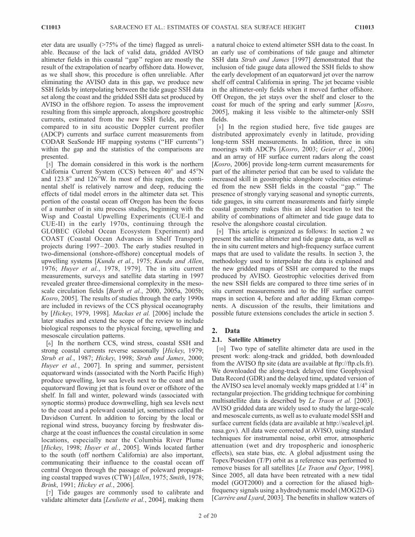
Table 4. Correlations and Standard Deviations of the Differences Between Velocities Estimated From SSH and HF Measurements and

ADCP Measurementsa

Name of Location

Vgeo+Ekman (z = 0)Versus HF Measurements

Vgeo+Ekman (z = 10 m)Versus ADCP

Vgeo Versus HFData (No Ekman)

Correlation(95% CL)

SD (Difference,in cm/s)

Correlation(95% CL)


Correlation(95% CL)


Newport, Oregon 0.93 (0.92) 6.4 0.92 (0.85) 7.7 0.92 (0.84) 8.1Coos Bay, Oregon 0.94 (0.75) 9.5 0.82 (0.62) 12 0.8 (0.67) 12.4Rogue River, Oregon 0.94 (0.75) 8.1 0.74 (0.55) 10.5 0.69 (0.55) 11.1

aOnly the meridional component of the velocities is considered. Geostrophic velocities (Vgeo) are estimated from the merged product between satelliteand tide gauge SSH. First column, name of nearest location; second column, surface (z = 0) Ekman currents are added to the Vgeo and compared to the HFcurrents; third column, Ekman currents at 10m depth (z = 10) are added to the Vgeo and compared to the ADCP currents at 10 m depth; fourth column,Vgeo are compared to the HF currents without adding any Ekman current.


13 of 20

C11013

Ekman components make a more significant contributionwhen compared to the HF surface current measurements.[40] We interpret the first two points above to suggest that

additional, realistic SSH data from within the coastal bandcan dramatically improve the gridded SSH and velocityfields in the same region. Although we use coastal tidegauge data in our region, improved retrievals of along-trackaltimeter data closer to the coast would provide a moregeneral solution to the problem, as discussed below. Thethird and fourth points above suggest that horizontal andvertical gradients of surface currents are more variable intime and space in coastal regions than assumed in oursimple example. Below we discuss these gradients, startingwith the vertical gradients of the Ekman currents andcontinuing with horizontal gradients of currents and SSH.This leads to the discussion of improved retrievals of thealong-track SSH data, which is the best hope for coastalaltimetry.

5.1. Estimates of Ekman Currents and Ekman Depths

[41] Our estimates of the Ekman currents assume a con-stant Ekman depth and a constant density. In reality, thesetwo parameters are not constant in space or time. The densityof seawater changes considerably in the region consideredhere, because of the sporadic presence of fresh water fromthe Columbia River in a surface layer. These fresher surface

layers only reduce the surface density by less than 1% of itsmean value [Huyer, 1977], producing little direct effect onthe Ekman current estimation (see equation (3)). However,they can provide a buoyant surface layer which requiresmore energy to mix vertically, reducing the Ekman depth andresulting in the concentration of the wind’s momentum in ashallow layer with greatly enhanced surface currents. Esti-mates of surface currents from the HF measurements can besubstituted for the surface Ekman currents and combinedwith estimates of the wind stress (from QuikSCAT) andgeostrophic currents (from altimeter SSH) to estimate the‘‘empirical’’ Ekman depth (d):

Vekm z ¼ 0ð Þ ¼ 1

r � d � f � ty � tx� �

; ð4Þ

d ¼ty � tx� �

r � f � VHF � Vgeo

� � ; ð5Þ

[42] Results of the empirical estimation of Ekman depth(Figure 10 (top)) are roughly consistent with the 15 m depthassumed during winter and autumn but show a lower valueduring spring and summer. Thus, use of a shallower Ekmandepth during spring and summer would result in stronger

Figure 10. At Coos Bay, (top) Ekman depth (m) and (bottom) meridional Ekman velocities (cm/s) asestimated from equation (5) (bold line) and as calculated using a constant Ekman depth of 15 m (thinline).


14 of 20

C11013

southward currents (Figure 10 (bottom)) that would bettermatch the observed currents. This would require indepen-dent estimates of Ekman depths, which cannot be obtainedfrom satellites but could come from several other sources.Seasonal changes in Ekman depths could be specified fromclimatologies of density profiles and mixed layer depths.For example, better estimates of temporally and spatially

varying density structure could be made from moorings andautonomous vehicle measurements, available from thecoastal monitoring systems planned by the U.S. IntegratedOcean Observing System (IOOS). Even more completeestimates of the 3-D density fields could come from coastalcirculation models run in the IOOS systems. However, thesemodels will eventually assimilate the altimeter SSH and HF

Figure 11. Comparison of alongshore currents (cm/s) at (top) Newport, (middle) Coos Bay, and(bottom) Rogue River. TG-only (blue line) currents are estimated fixing the SSH (z = 0) 40 km offshore,i.e., only considering the forcing of the TG. The result obtained by merging TG and satellite data and asestimated by the ADCP at 10 m depth are displayed with red and black lines, respectively. Correlationsand standard deviations of the difference obtained between time series are presented in Table 5.


15 of 20

C11013

surface velocity fields, producing more realistic velocityfields that make the calculation of Ekman and geostrophicvelocities from the satellite data a moot point.

5.2. Estimation of the Alongshore Current by TGsOnly: Variability in Large-Scale Coastal SSH Gradients

[43] It is natural to ask how much of the alongshorevelocity and transport in the gap region is contributed bySSH variations in the tide gauge record alone, compared tothe combination of tide gauges and offshore altimeter SSHfields. Huyer et al. [1978] found that alongshore currentsover the Oregon shelf vary simultaneously with tide gaugeSSH measurements at the coast. Assuming linear or expo-nential decays of the sea level from the coast, Kundu et al.[1975] and Huyer et al. [1978] estimate an offshore lengthscale L over which the geostrophic velocities correctlyapproximate the alongshore currents. Huyer et al. [1978]found that L is larger in winter than in spring and summer,the value depending on the approximation considered(linear or exponential). Considering the linear approxima-tion, values are 52 km for winter, between 17 and 35 km forspring and 30–40 km for summer [Huyer et al., 1978]. Thisseasonal variability is consistent with changes in the Rossbyradius of deformation, which is minimum during summerand maximum in winter, because of seasonal changes in thestratification and mixed layer depth.[44] We test these relationships with the present data,

using a constant offshore length scale (L) and a SSH profilethat decays linearly from the value measured at the tidegauge to 0 cm at L = 40 km. We compare the resultinggeostrophic currents to those produced by the TG andaltimeter combination and those measured by the ADCPslocated over the shelves at Newport (8 years of data), CoosBay (5 years of data) and Rogue River (4 years of data).Differences between the TG-only and ADCP currents are, ingeneral, small in spring-summer and large in winter, con-sistent with results from Huyer et al. [1978]. The largeoverestimates of poleward currents by the TG-only timeseries in winter are consistent with the fact that the effectiveL is larger in winter and values of SSH are not zero 40 kmoffshore. The altimeter provides better estimates of SSH at40 km offshore during winters. The underestimates ofequatorward currents by the combination of TG and altim-eter data in spring and early summer are due to theunderestimate of the SSH gradients associated with theupwelling jet. The true SSH gradients in summer occurover much shorter distances across the jet (see section 5.3).When the strong SSH gradient associated with the jet movesoffshore of the shelf and current meter in late summer and

autumn [Strub and James, 2000], the combination of TGand altimeter data produces a better estimate of the mea-sured alongshore current than the 40 km linear gradientusing only the TG data.[45] The above comparisons are quantified by values of

the standard deviations of the difference between the ADCPand calculated alongshore velocities, along with their cor-relations. At Newport, with the longest time series, ouraltimeter-TG estimates of SSH and geostrophic currentsproduce values of 11.6 cm/s (standard deviation of differ-ence) and 0.83 (correlation coefficient, see Figure 6 andTable 3). Use of the TG only SSH with L = 40 km results invalues of 15.9 cm/s and 0.79 (see Figure 11 and Table 5).Thus, using the altimeter data on the offshore boundary ofthe 40 km gap region improves the results. The sametendency is found at Rogue River and Coos Bay, i.e.,correlations are very similar but standard deviations of thedifferences present lower values when TGs are merged withsatellite SSH data (Table 5).[46] Using the measured ADCP time series of alongshore

velocities, we can find an optimal value of L to use in theTG-only calculations, to best match the measurements. Thestandard deviation of the difference between the measuredADCP alongshore currents at 10 m depth and the TG onlycalculation decreases exponentially as L increases to adistance of 70 km from the coast, increasing slowly for Llarger than 70 km. With L = 70 km, the standard deviationof the difference between the ADCP and TG-only calcula-tion is 11.3 cm/s and the correlation coefficient is the sameas with L = 40 km. The decrease in standard deviation of thedifferences is due to a decrease in overestimation ofalongshore velocities in winter and a smaller increase inunderestimates of velocities in summer.[47] Although correlations of low-frequency signals in

the time series are dominated by seasonal cycles, significantcorrelations are found at higher frequencies (periods ofweeks). To demonstrate this, we estimate the correlationsbetween unfiltered, low-pass filtered and high-pass filteredtime series of the SAT+TG and TG only versus ADCP data,respectively. Time series are low-pass filtered using a 90-dayperiod as the cutoff frequency, separating seasonal (andlonger) variability from intraseasonal variability. The high-frequency time series are constructed as the differencebetween the unfiltered and the low-pass filtered time series.Results (see Table 5) indicate that while correlation valuesare similar for low- and high-frequency time series, only thehigh-frequency signals are significantly correlated (wellabove the 95% significance level). The lack of significance

Table 5. Correlations and Standard Deviations of the Difference Between TG-Only, SAT+TG, and ADCP Velocity Time Series When

They Are Unfiltered, Low-Pass Filtered, and High-Pass Filtereda

LocationInstrumentsCompared

Unfiltered Low-Frequency High-Frequency

Correlation(95% CL)


Correlation(95% CL)


Correlation(95% CL)


Newport SAT+TG versus ADCP 0.83(0.75) 11.6 0.82(0.8) 9.6 0.77(0.2) 6.4Newport TG-only versus ADCP 0.79(0.7) 15.9 0.75(0.8) 16.9 0.76(0.2) 6.6Coos Bay SAT+TG versus ADCP 0.73(0.6) 12.6 0.77(0.8) 8.4 0.7(0.29) 9.2Coos Bay TG-only versus ADCP 0.68(0.6) 18.5 0.73(0.8) 16 0.71(0.2) 8.4Rogue River SAT+TG versus ADCP 0.77(0.58) 11.9 0.82(0.8) 7.3 0.75(0.3) 9.4Rogue River TG-only versus ADCP 0.74(0.6) 15.5 0.8(0.88) 13 0.75(0.3) 7.8

aSAT+TG, merged product between satellite and tide gauge sea level anomaly.


16 of 20

C11013

for the low-frequency signals is due to the fact that they aredominated by the seasonal cycles, which have a low numberof degrees of freedom over the 4–8 year time series (withlower significance levels for high correlations).[48] Table 5 also shows that the standard deviations of the

differences of the unfiltered and low-pass filtered time seriesare lower (by at least 3.6 cm/s) when the satellite informa-tion is interpolated to the TGs rather than when the TG onlyare considered. This supports the previous conclusionthat the altimeter data provides offshore information thatcompensates for the seasonally changing length scale forthe offshore decay of the coastal SSH, as measured by thetide gauges. The contributions of the offshore altimeterdata are more important on the seasonal and longer time-scales than on the intraseasonal timescales. This is demon-strated by the fact that the standard deviations of thedifference for the high-frequency components presentalmost no differences (with or without altimeter data). Thisreflects the fact that present altimeters do not adequatelysample synoptic and intraseasonal timescales. It alsoemphasizes the need to integrate altimeter data with obser-vations from instruments that do sample higher-frequencytimescales (tide gauges, coastal radars, moorings, etc.) forcoastal observing systems.

5.3. Interpolation of SSH in the Gap Region:Variability in Small-Scale Coastal SSH Gradients andthe Path Forward for Improved Coastal Fields

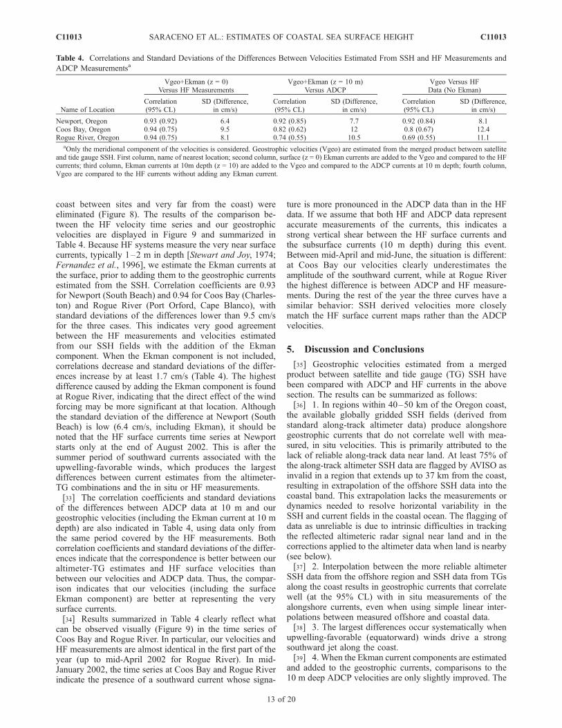
[49] The above discussion suggests that the greatestsource of error in the new estimates of alongshore velocitymay come from our use of a linear interpolation of SSH inthe gap region. In situ observations show that duringupwelling favorable winds the dynamic height does notdecay linearly in the gap region. Instead, the slope of theSSH in the gap region is concentrated, on average, around anarrower region of maximum slope [Fleischbein et al.,2005, Figure 19], and the equatorward alongshore surfaceflow is often concentrated into a current jet [e.g., Kosro,2005], whose core location changes with time. Averaged

over weeks to months, the slope of the SSH resembles a‘‘cosine-like’’ decay of SSH, with maximum slope and astrong jet in the middle of the gap region, as depictedschematically in Figure 12. This observation was, in fact,the motivation for the location of the ADCP mooring atmidshelf off Newport.[50] At any given time, however, even narrower coastal

jets, filaments and other small-scale structures in SSH andvelocity are found routinely in coastal regions [Kosro, 2005;Barth et al., 2005a, 2005b; Fleischbein et al., 2005]. Anexample is shown from the Oregon coast during June 2005,in Figure 13. A band of colder SST values is seen next tothe coast south of 45�N on 29 June. Two altimeter tracks areshown (straight lines) ascending from SW to NE (27 June)and descending from the NW to SE (28 June). SSH datafrom these tracks are recovered by substituting a model-derived ‘‘wet troposphere atmospheric correction’’ for thestandard correction from the onboard microwave radiome-ter, which does not produce usable data east of �125�W(see below). Along the descending (NE–SW) track, SSHvalues (the fluctuating lines) drop approximately 12 cm asthe altimeter approaches the coast at �44.7�N, 124.8�W,and drop again �25 cm near 44.3�N, 124.4�W. The second,larger drop in SSH occurs approximately where the altim-eter track crosses from warmer to colder water. The SSHvalues represent the vertically integrated specific volume ofthe water column (here controlled primarily by the temper-ature), similar to dynamic heights. From past measurements,we expect a strong jet along the SST/SSH front. The smallerdrop in SSH, farther offshore, represents another subsurfacedensity front that is covered by a surface layer of warm SSTand should correspond to a weaker jet. These fronts dem-onstrate the true nature of the SSH and current fields at anygiven time, which are poorly resolved by a linear gradient ofSSH between the coast and the offshore region. However,the geostrophic alongshore transport integrated across thegap is accurately portrayed, regardless of the shape of theSSH field in the gap region, and the linear interpolation

Figure 12. Schematic representation of SSH (bold lines) and corresponding geostrophic velocities (thinlines) of (left) a cosine-like decay of SSH and (right) a linear decay in the gap region. The position of theADCP is indicated.


17 of 20

C11013

provides a large increase in skill compared with the original,extrapolated AVISO product.[51] Our interpolation of SSH between valid offshore

altimeter data and coastal tide gauges represents a first stepin improving the SSH fields in coastal regions. It primarilydemonstrates that more realistic SSH data from within thecoastal region are able to improve altimeter estimates of

SSH and surface currents within approximately 40 km ofland. The use of tide gauge data and an assumed shape forthe interpolated SSH profile (linear, cosine or otherwise)across the coastal gap is a weakness of the present analysis,motivated by the lack of measurements in the gap regioninterior. For many coastal locations, an additional limitationfor this technique is the lack of a relatively dense array ofwell-maintained tide gauges, with long and consistent timeseries.[52] The more general solution to the problem of obtain-

ing improved fields of SSH in coastal regions requires bettermethods for retrieving the along-track altimeter SSH data inthose regions. This will replace the use of tide gauges, withglobal coverage to within approximately 5 km of land.However, modification are needed for the methods used toretrieve the altimeter’s reflected radar signal and to estimate‘‘corrections’’ to the path delay caused by atmosphericconstituents and surface effects. Close to the coast (10–20 km), land contaminates the actual reflected altimetricradar signal. Advanced methods for tracking the reflectionpoint of the radar signal from the ocean and land surfacesare needed, as described by Fenoglio-Marc et al. [2007].Farther from the coast, the large footprint of the onboardmicrowave radiometers used to estimate the wet tropospher-ic path delay (because of vertically integrated atmosphericwater vapor) intersects land and creates a data gap withinapproximately 50 km of land. Alternative estimates for thewet tropospheric correction are provided by atmosphericmodels [Madsen et al., 2007], as used in Figure 13,although they may not resolve sharp gradients in atmo-spheric moisture, associated with fronts near the coast.Modified algorithms for the onboard microwave radiometerare being explored, as described by Desportes et al. [2007].[53] Algorithms to correct for these and other atmospheric

and surface effects in coastal regions are the subject ofseveral international initiatives, including ALTICORE[Vignudelli et al., 2008; Bouffard et al., 2008] (informationavailable at www.alticore.eu), COASTALT [Cipollini et al.,2008] (data are available at www.coastalt.eu), and PIS-TACH [Lambin et al., 2008]. Improvements in methods forcoastal altimetry are also being discussed in an ongoingseries of workshops [Smith et al., 2008]. Our resultsdemonstrate that inclusion of more realistic SSH data (fromtide gauges, altimeter tracks or other sources) in producinggridded SSH fields will result in improved estimates ofsurface currents in these coastal regions, where society’suse of the ocean continues to increase.

5.4. Summary

[54] The present work shows that the combination of SSHdata from tide gauges and satellite altimeter fields improvesthe altimeter SSH fields within 40–50 km of the coast andincreases the accuracy of the alongshore surface velocitiesderived from those fields. We also point out that compactstructures such as coastal jets are only partially representedusing the linear interpolation techniques employed here,causing higher differences between SSH-derived velocitiesand in situ measurements in summer over the shelf offOregon. These jets are narrower than can be represented bya linear interpolation of SSH from 40 km offshore to the tidegauges at the coast. To improve the representation of thevelocity structure in the 40 km next to the coast, methods

Figure 13. SST (colors) from the Advanced Very HighResolution Radiometer and along-track SSH from theJason-1 altimeter during 27–29 June 2005. A wet tropo-sphere correction from the European Center for Medium-range Weather Forecasting model has been substituted forthe standard correction to retrieve SSH data east of 125�W.Clouds are indicated by gray and speckled patterns in theoffshore and northern regions. The region next to the coastsouth of the Columbia River (46.3�N) is relatively cloudfree. Altimeter track paths are the straight lines (redindicates offshore, and black indicates east of the trackcrossover at 124.7�W); along-track SSH values are shownby the solid traces fluctuating above and below the tracks(10-cm-scale distance shown over land). Low-SSH valuesare indicated when the SSH traces are offshore (left) of thetracks. Sharp drops in SSH (�12 cm and �25 cm) are seenalong the track moving from NW to SE at �44.7�N,124.8�W and 44.3�N, 124.4�W, respectively.


18 of 20

C11013

must be found to retrieve the actual along-track altimeter SSHdata in that region. These data can then be used in two ways:[55] 1. They can be used as inputs to advanced gridding

techniques, such as employed by AVISO, to produce morerealistic SSH fields. Surface velocity fields can be producedfrom the SSH fields, with or without the addition of Ekmancomponents [Johnson et al., 2007; Sudre andMorrow, 2008].[56] 2. The same SSH data (either along-track or gridded)

can be assimilated into dynamical models of coastal oceancirculation (A. L. Kurapov et al., Representer-based analy-ses in the coastal upwelling system, submitted to Dynamicsof Atmospheres and Oceans, 2008). However, our resultsshow that the presently available gridded SSH fields,without the inclusion of more realistic SSH data (from tidegauges or improved along-track altimeter data), do notaccurately represent details of the circulation within 40–50 km of the coast and should not be assimilated intocoastal models.[57] Ignoring spatial details of the coastal circulation, for

regions with narrow shelves, the spatially integrated geo-strophic alongshore transport in the region within 40 km ofthe coast depends only on the difference of SSH across thatregion (not on the particular shape of the SSH). Thus, thetechniques described here can be used to construct a 15 yearindex of the alongshore transport within �40–50 km of thecoast, anywhere that a sufficiently long record of SSH froma well-maintained tide gauge exists. This index may be usedfor studies of climatic variability in water mass character-istics, plankton species, etc., caused by changes in along-shore transports.

[58] Acknowledgments. Support for M.S., P.T.S., and P.M.K. wasprovided by NOAA/NESDIS through the Cooperative Institute for Ocean-ographic Satellite Studies (NOAA grant NA03NES4400001) and the U.S.GLOBEC project (NSF grants OCE-0000733, OCE-0000734, and OCE-0000900). Additional support for P.T.S was provided by NASA/JPL (grantJPL-1206714-OSTM). The altimeter products were produced by SSALTO/DUACS (Segment Sol multimissions d’ALTimetrie, d’Orbitographie et delocalization precise/Data Unification Altimeter Combination System) anddistributed by AVISO with support from CNES (Centre National de laRecherche Scientifique). We thank S. Ramp (NPS) and B. Hickey (UW) formaking available processed measurements from their GLOBEC moorings atRogue River and Coos Bay, respectively. Comments by three anonymousreviewers and the editor greatly improved the paper. This is contribution 604of the U.S. GLOBEC program, jointly funded by the National ScienceFoundation and the National Oceanic and Atmospheric Administration.

ReferencesAllen, J. S. (1975), Coastal trapped waves in a stratified ocean, J. Phys. Ocea-nogr., 5, 300–325, doi:10.1175/1520-0485(1975)005<0300:CTWIAS>2.0.CO;2.

Barber, C. B., D. P. Dobkin, and H. T. Huhdanpaa (1996), The QuickhullAlgorithm for convex hulls, Trans. Math. Software, 22(4), 469–483,doi:10.1145/235815.235821.

Barrick, D. E., M. W. Evans, and B. L. Weber (1977), Ocean surfacecurrents mapped by radar, Science, 198, 138–144, doi:10.1126/science.198.4313.138.

Barth, J. A., S. D. Pierce, and R. L. Smith (2000), A separating coastalupwelling jet at Cape Blanco, Oregon and its connection to the CaliforniaCurrent System, Deep Sea Res., Part II, 47, 783–810, doi:10.1016/S0967-0645(99)00127-7.

Barth, J. A., S. D. Pierce, and R. M. Castelao (2005a), Time-dependent,wind-driven flow over a shallow midshelf submarine bank, J. Geophys.Res., 110, C10S05, doi:10.1029/2004JC002761.

Barth, J. A., S. D. Pierce, and T. J. Cowles (2005b), Mesoscale structureand its seasonal evolution in the northern California Current System,Deep Sea Res., Part II, 52, 5–28, doi:10.1016/j.dsr2.2004.09.026.

Brink, K. H. (1991), Coastal-trapped waves and wind-driven currents overthe continental shelf, Annu. Rev. Fluid Mech., 23, 389–412, doi:10.1146/annurev.fl.23.010191.002133.

Bouffard, J., S. Vignudelli, M. Herrmann, F. Lyard, P. Marsaleix, Y. Menard,and P. Cipollini (2008), Comparison of ocean dynamics with aregional circulation model and improved altimetry in the northwesternMediterranean, Terr. Atmos. Oceanic Sci., 19, 117–133, doi:10.3319/TAO.2008.19.1-2.117(SA).

Carrere, L., and F. Lyard (2003), Modeling the barotropic response of theglobal ocean to atmospheric wind and pressure forcing—Comparisonswith observations, Geophys. Res. Lett., 30(6), 1275, doi:10.1029/2002GL016473.

Chelton, D., and M. G. Schlax (2003), The accuracies of smoothed seasurface height fields constructed from tandem satellite altimeter datasets,J. Atmos. Oceanic Technol., 20, 1276 – 1302, doi:10.1175/1520-0426(2003)020<1276:TAOSSS>2.0.CO;2.

Cipollini, P., J. Gomez-Enri, C. Gommenginger, C.Martin-Puig, S.Vignudelli,P. Woodworth, and J. Benveniste (2008), Developing radar altimetry inthe oceanic coastal zone: The COASTALT project, paper presented at theGeneral Assembly 2008, Eur. Geosci. Union, Vienna, 13–18 Apr.

Cleveland, W. S., and S. Devlin (1988), Locally weighted regression: Anapproach to regression analysis by local fitting, J. Am. Stat. Assoc., 83,596–610, doi:10.2307/2289282.

Davis, R. E. (1976), Predictability of sea surface temperature and sea levelpressure anomalies over the North Pacific Ocean, J. Phys. Oceanogr., 6,249–266, doi:10.1175/1520-0485(1976)006<0249:POSSTA>2.0.CO;2.

Delaunay, B. (1934), Sur la sphere vide, Otdelenie Mat. EstestvennykhNauk, 7, 793–800.

Deng, X., and W. E. Featherstone (2006), A coastal retracking systemfor satellite radar altimeter waveforms: Application to ERS-2 aroundAustralia, J. Geophys. Res., 111, C06012, doi:10.1029/2005JC003039.

Desportes, C., E. Obligis, and L. Eymard (2007), On the wet troposphericcorrection for altimetry in coastal regions, IEEE Trans. Geosci. RemoteSens., 45(7), 2139–2142, doi:10.1109/TGRS.2006.888967.

Ekman, V. W. (1905), On the influence of the Earth’s rotation on oceancurrents, Arch. Math. Astron. Phys., 2, 11.

Fenoglio-Marc, L., S. Vignudelli, A. Humbert, P. Cipollini, M. Fehlau, andM. Becker (2007), An assessment of satellite altimetry in proximity of theMediterranean coastline, paper presented at 3rd ENVISAT Symposium,Eur. Space Agency, Montreux, Switzerland.

Fernandez, D. M., J. F. Vesecky, and C. C. Teague (1996), Measurements ofupper ocean surface current shear with high-frequency radar, J. Geophys.Res., 101, 28,615–28,625, doi:10.1029/96JC03108.

Fleischbein, J. H., A. Huyer, P. M. Kosro, R. L. Smith, and P. A. Wheeler(2005), Upper ocean water properties and currents along paired sectionsin the Northern California Current, summer 1998–2003, Data Rep. 201,Coll. of Oceanic and Atmos. Sci., Oreg. State Univ., Corvallis, Oreg.

Geier, S. L., B. M. Hickey, S. R. Ramp, P. M. Kosro, N. B. Kachel, andF. Bahr (2006), Interannual variability in water properties and velocityin the U. S. Pacific Northwest coastal zone, EOS Trans. AGU, 87(36),Ocean Sci. Meet. Suppl., Abstract OS36D–23.

Harms, S., and C. Winant (1994), Synthetic subsurface pressure derivedfrom bottom pressure and tide gauge observations, J. Atmos. OceanicTechnol., 11, 1625 –1637, doi:10.1175/1520-0426(1994)011<1625:SSPDFB>2.0.CO;2.

Hickey, B. M. (1979), The California Current System—Hypotheses andfacts, Prog. Oceanogr., 8, 191–279, doi:10.1016/0079-6611(79)90002-8.

Hickey, B. M. (1998), Coastal oceanography of western North America fromthe tip of Baja California to Vancouver Island, in The Sea, edited by A. R.Robinson and K. H. Brink, pp. 345–393, John Wiley, New York.

Hickey, B. M., A. MacFadyen, W. Cochlan, R. Kudela, K. Bruland, andC. Trick (2006), Evolution of chemical, biological, and physical waterproperties in the northern California Current in 2005: Remote or local windforcing?, Geophys. Res. Lett., 33, L22S02, doi:10.1029/2006GL026782.

Huyer, A. (1977), Seasonal variation in temperature, salinity, and densityover the continental shelf off Oregon, Limnol. Oceanogr., 22(3), 442–453.

Huyer, A., R. L. Smith, and E. J. C. Sobey (1978), Seasonal differencesin low-frequency currents fluctuations over the Oregon continental shelf,J. Geophys. Res., 83, 5077–5089, doi:10.1029/JC083iC10p05077.

Huyer, A., E. J. C. Sobey, and R. L. Smith (1979), The spring transition incurrents over the Oregon continental shelf, J. Geophys. Res., 84, 6995–7011, doi:10.1029/JC084iC11p06995.

Huyer, A., J. H. Fleischbein, J. Keister, P. M. Kosro, N. Perlin, R. L. Smith,and P. A. Wheeler (2005), Two coastal upwelling domains in the northernCalifornia Current system, J. Mar. Res., 63, 901–929, doi:10.1357/002224005774464238.

Huyer, A., P. A.Wheeler, P. T. Strub, R. L. Smith, R. Letelier, and P.M. Kosro(2007), The Newport Line off Oregon—Studies in the Northeast Pacific,Prog. Oceanogr., 75, 126–160, doi:10.1016/j.pocean.2007.08.003.

Johnson, E. S., F. Bonjean, G. S. E. Lagerloef, J. T. Gunn, and G. T.Mitchum (2007), Validation and error analysis of OSCAR sea surface


19 of 20

C11013

currents, J. Atmos. Oceanic Technol., 24, 688 – 701, doi:10.1175/JTECH1971.1.

Kelly, K. A., R. C. Beardsley, R. Limeburner, K. H. Brink, J. D. Paduan,and T. K. Chereskin (1998), Variability of the near-surface eddy kineticenergy in the California Current based on altimetric, drifter, and mooredcurrent data, J. Geophys. Res., 103, 13,067 –13,084, doi:10.1029/97JC03760.

Kosro, P. M. (2003), Enhanced southward flow over the Oregon shelf in2002: A conduit for subarctic water, Geophys. Res. Lett., 30(15), 8023,doi:10.1029/2003GL017436.

Kosro, P. M. (2005), On the spatial structure of coastal circulation offNewport, Oregon, during spring and summer 2001, in a region of varyingshelf width, J. Geophys. Res., 110, C10S06, doi:10.1029/2004JC002769.

Kosro, P. M. (2006), Charting the time-varying surface circulation offOregon, Eos Trans. AGU, 87(36), Ocean Sci. Meet. Suppl., AbstractOS23B–05.

Kundu, P. K., and J. S. Allen (1976), Some three dimensional character-istics of low-frequency current fluctuations near the Oregon coast, J.Phys. Oceanogr., 6, 181–199, doi:10.1175/1520-0485(1976)006<0181:STDCOL>2.0.CO;2.

Kundu, P. K., J. S. Allen, and R. L. Smith (1975), Modal decomposition ofthe velocity field near the coast of Oregon, J. Phys. Oceanogr., 5, 683–704, doi:10.1175/1520-0485(1975)005<0683:MDOTVF>2.0.CO;2.

Lambin, J., A. Lombard, and N. Picot (2008), CNES initiative for altimeterprocessing in coastal zone: PISTACH, paper presented at the First CoastalAltimeter Workshop, Centre Natl. D’Etud. Spatiales, Silver Spring, Md.,5–7 Feb.

Le Traon, P. Y., and G. Dibarboure (2002), Velocity mapping capabilities ofpresent and future altimeter missions: The role of high frequency signals,J. Atmos. Oceanic Technol., 19, 2077 – 2088, doi:10.1175/1520-0426(2002)019<2077:VMCOPA>2.0.CO;2.

Le Traon, P. Y., and F. Ogor (1998), ERS-1/2 orbit improvement usingTopex/POSEIDON: The 2 cm challenge, J. Geophys. Res., 103, 8045–8058, doi:10.1029/97JC01917.

Le Traon, P. Y., Y. Faugere, F. Hernandez, J. Dorandeu, F. Mertz, andM. Ablain (2003), Can we merge GEOSAT follow-on with Topex/Poseidon and ERS-2 for an improved description of the ocean cir-culation?, J. Atmos. Oceanic Technol., 20, 889–895, doi:10.1175/1520-0426(2003)020<0889:CWMGFW>2.0.CO;2.

Leeuwenburgh, O., and D. Stammer (2002), Uncertainties in altimetry-basedvelocity estimates, J. Geophys. Res., 107(C10), 3175, doi:10.1029/2001JC000937.

Lentz, S. (1993), The accuracy of tide-gauge measurements at subtidalfrequencies, J. Atmos. Oceanic Technol., 10, 238–245, doi:10.1175/1520-0426(1993)010<0238:TAOTGM>2.0.CO;2.

Leuliette, E. W., R. S. Nerem, and G. T. Mitchum (2004), Calibration ofTopex/Poseidon and Jason altimeter data to construct a continuous recordof mean sea level change, Mar. Geod., 27, 79 – 94, doi:10.1080/01490410490465193.

Lillibridge, J. (2005), Coastal altimetry challenges, paper presented at ScienceReview Meeting, Coop. Inst. for Oceanogr. Satell. Stud., Corvallis, Oreg.

Lipa, B. J., and D. E. Barrick (1983), Least-squares methods for theextraction of surface currents from CODRA crossed-loop data: Applica-tion at ARSLOE, IEEE J. Oceanic Eng., 8, 226–253, doi:10.1109/JOE.1983.1145578.

Mackas, D. L., P. T. Strub, A. C. Thomas, and V. Montecino (2006), Easternocean boundaries—Pan regional overview, in The Sea: TheGlobal CoastalOcean, Interdisciplinary Regional Studies and Syntheses: Pan-RegionalSyntheses and the Coasts of North and South America and Asia, editedby A. R. Robinson and K. H. Brink, pp. 21–60, Harvard Univ. Press,Cambridge, Mass.

Madsen, K. S., J. L. Høyer, and C. C. Tscherning (2007), Near-coastalsatellite altimetry: Sea surface height variability in the North Sea–BalticSea area, Geophys. Res. Lett., 34, L14601, doi:10.1029/2007GL029965.

Manzella, G. M. R., G. Borzelli, P. Cipollini, T. H. Guymer, H. M. Snaith,and S. Vignudelli (1997), Potential use of satellite data to infer the cir-culation dynamics in a marginal area of the Mediterranean Sea, Rep. ESASP-414, Eur. Space Agency, Noordwijk, Netherlands.

Marcotte, D. (1991), Cokriging with MATLAB, Comput. Geosci., 17(9),1265–1280, doi:10.1016/0098-3004(91)90028-C.

Pascual, A., Y. Faugere, G. Larnicol, and P.-Y. Le Traon (2006), Improveddescription of the ocean mesoscale variability by combining four satellitealtimeters, Geophys. Res. Lett., 33, L02611, doi:10.1029/2005GL024633.

Pascual, A., M. I. Pujol, G. Larnicol, P. Y. Le Traon, and M. H. Rio (2007),Mesoscale mapping capabilities of multisatellite altimeter missions: Firstresults with real data in the Mediterranean, J. Mar. Syst., 65(1–4), 190–211, doi:10.1016/j.jmarsys.2004.12.004.

Smith, R. L. (1978), Poleward propagating perturbations in currents and sealevel along the Peru coast, J. Geophys. Res., 83, 6083–6092, doi:10.1029/JC083iC12p06083.

Smith, W. H. F., P. T. Strub, and L. Miller (2008), First coastal altimetryworkshop held, Eos Trans. AGU, 89(40), doi:10.1029/2008EO400008.

Stewart, R. H., and J. W. Joy (1974), HF radio measurements of surfacecurrents, Deep Sea Res. Oceanogr. Abstr., 21, 1039–1049.

Strub, P. T., and C. James (1997), Satellite comparisons of Eastern Bound-ary Currents: Resolution of circulation features in ‘‘coastal’’ oceans,paper presented at Monitoring the Oceans in the 2000s: An IntegratedApproach, Centre Natl. d’Etud. Spatiale, Biarritz, France.

Strub, P. T., and C. James (2000), Altimeter-derived variability of surfacevelocities in the California Current System: 2. Seasonal circulation andeddy statistics, Deep Sea Res., Part II, 47, 831–870, doi:10.1016/S0967-0645(99)00129-0.

Strub, P. T., and C. James (2002a), Altimeter-derived surface circulation inthe large-scale NE Pacific gyres — Part 1. Seasonal variability, Prog.Oceanogr., 53, 163–183, doi:10.1016/S0079-6611(02)00029-0.

Strub, P. T., and C. James (2002b), The 1997–1998 oceanic El Nino signalalong the southeast and northeast Pacific boundaries—An altimetric view,Prog. Oceanogr., 54, 439–458, doi:10.1016/S0079-6611(02)00063-0.

Strub, P. T., J. S. Allen, A. Huyer, and R. C. Beardsley (1987), Seasonalcycles of currents, temperatures, winds, and sea level over the NortheastPacific Continental Shelf: 35�N to 48�N, J. Geophys. Res., 92, 1507–1526, doi:10.1029/JC092iC02p01507.

Sudre, J., and R. A. Morrow (2008), Global surface currents: A high-resolution product for investigating ocean dynamics, Ocean Dyn., 58,101–118, doi:10.1007/s10236-008-0134-9.

Vignudelli, S., P. Cipollini, M. Astraldi, G. P. Gasparini, and G. Manzella(2000), Integrated use of altimeter and in situ data for understanding thewater exchanges between the Tyrrhenian and Ligurian seas, J. Geophys.Res., 105, 19,649–19,664, doi:10.1029/2000JC900083.

Vignudelli, S., P. Cipollini, L. Roblou, F. Lyard, G. P. Gasparini, G.Manzella,and M. Astraldi (2005), Improved satellite altimetry in coastal systems:Case study of the Corsica Channel (Mediterranean Sea), Geophys. Res.Lett., 32, L07608, doi:10.1029/2005GL022602.

Vignudelli, S., P. Berry, and L. Roblou (2008), Satellite altimetry nearcoasts—Current practices and a look at the future, paper presented at15 Years of Progress in Radar Altimetry, Eur. Space Agency, Venice,Italy, 6 Oct.

Volkov, D. L., G. Larnicol, and J. Dorandeu (2007), Improving the qualityof satellite altimetry data over continental shelves, J. Geophys. Res., 112,C06020, doi:10.1029/2006JC003765.

��P. M. Kosro and P. T. Strub, College of Oceanic and Atmospheric

Sciences, Oregon State University, 104 COAS Administration Building,Corvallis, OR 97331-5503, USA.M. Saraceno, Centro de Investigaciones del Mar y la Atmosfera, Ciudad

Universitaria, Intendente Guiraldes 2160, Pab. II, 2do piso, Ciudad deBuenos Aires, C1428EGA, Argentina. ([email protected])


20 of 20

C11013

estimates of sea surface height and near-surface...

Documents