essential dynamics for developing models for control of

Essential Dynamics for Developing Models forControl of Connected and Automated ElectriedVehicles: Part A - PowertrainSadra Hemmati ( [email protected] )

Michigan Tech https://orcid.org/0000-0003-0793-4677Rajeshwar yadav

GKN DrivelineKaushik Surresh

Michigan Technological UniversityDarrell Robinette

Michigan Technological UniversityMahdi Shahbakhti

University of Alberta

Research Article

Keywords: Connected and Automated Vehicles, Automotive Control, Energy Eciency

Posted Date: May 18th, 2021

DOI: https://doi.org/10.21203/rs.3.rs-536651/v1

License: This work is licensed under a Creative Commons Attribution 4.0 International License. Read Full License

https://doi.org/10.21203/rs.3.rs-536651/v1

mailto:[email protected]

https://orcid.org/0000-0003-0793-4677

https://doi.org/10.21203/rs.3.rs-536651/v1

https://creativecommons.org/licenses/by/4.0/

ESSENTIAL DYNAMICS FOR DEVELOPING MODELS FOR CONTROL OF

CONNECTED AND AUTOMATED ELECTRIFIED VEHICLES: PART A - POWERTRAIN

Sadra Hemmati

Michigan Technological University

Houghton, Michigan 49931

Email: [email protected]

Rajeshwar Yadav

GKN Driveline


Kaushik Surresh



Darrell Robinette



Mahdi Shahbakhti

University of Alberta

Edmonton, Alberta, Canada


ABSTRACT

Connected and Automated Vehicles (CAV) technology

presents significant opportunities for energy saving in the trans-

portation sector. CAV technology forecasts vehicle and power-

train power needs under various terrain, ambient, and traffic

conditions. Even though the CAV technology is applicable to

both conventional and electrified powertrains, the energy sav-

ing opportunities are more apparent when the CAVs are Hybrid

Electric Vehicles (HEVs). This is because of the flexibility in the

vehicle powertrain and possibility of choosing optimum power-

train modes based on the predicted traction power needs. In this

paper, the powertrain dynamics essential for developing power-

train controllers for a class of connected HEVs is presented. To

this end, control-oriented powertrain dynamic models for a test

vehicle consisting of full electric, hybrid, and conventional en-

gine operating modes are developed. The resulting powertrain

model can forecast vehicle traction torque and energy consump-

tion for the specified prediction horizon of the test vehicle. The

model considers different operating modes and associated en-

ergy penalty terms for mode switching. Thus, the vehicle con-

troller can determine the optimum powertrain mode, torque, and

speed for forecasted vehicle operation via utilizing connectivity

data. The powertrain model is validated against the experimen-

tal data and shows prediction error of less than 5% for predicting

vehicle energy consumption.

1 Introduction

With increased penetration of electrification and connectiv-

ity technologies in the market, the potential for intelligent and

energy-efficient transportation becomes more salient [1]. Ac-

cording to the U.S. Energy Information Administration (EIA)

2020 outlook for the transportation industry, light-duty hybrid

electric vehicle sales in the U.S. are predicted to increase 3.1%

per year, rising to a projected sales of more than 900,000 vehi-

cles in 2050, while battery electric vehicle (BEV) sales will in-

crease by 6% per year on average [2]. HEV/ BEV powertrain is a

1 Copyright © by ASME

complex system consisting of numerous sub-systems. To ensure

good fuel economy and drivability, it is imperative to model and

characterize the dynamic interactions among the components. To

establish and understand these interactions, physical prototyping

and testing prove to be too expensive [3], whereas modeling and

simulation is considered cost-effective and time-saving for mod-

eling and control of connected electrified powertrains [4]. Con-

nectivity facilitates forecasting future tractive and thermal loads

and power demands to the vehicle. This can be utilized for intel-

ligent control and energy saving [1]. Even though CAV informa-

tion is helpful for the energy-efficient operation of conventional

vehicles, EVs, and HEVs, the energy saving opportunities are

more apparent when the CAVs are HEV due to flexibility in se-

lecting the vehicle powertrain operating modes. In this paper,

the powertrain dynamics that should be modeled for developing

powertrain controller for connected vehicles is presented, with

emphasis on connected HEVs (CHEVs).

Important Dynamics for Vehicle Controls to Enable

Energy Saving in Hybrid Electric CAVs

- Mode switching

including clutch

and power split

mechanisms

- ICE transients

- E-motor and ICE

efficiency maps

Powertrain

Dynamics

- Vehicle velocity

profiling

- Road gradient

effects and

predictive energy

consumption

- Vehicle

platooning

Vehicle

Dynamics

- Vehicle cold-start

(ICE coolant &

aftertreatment

systems)

- Battery thermal

management

- Cabin thermal air

conditioning

Thermal

Dynamics

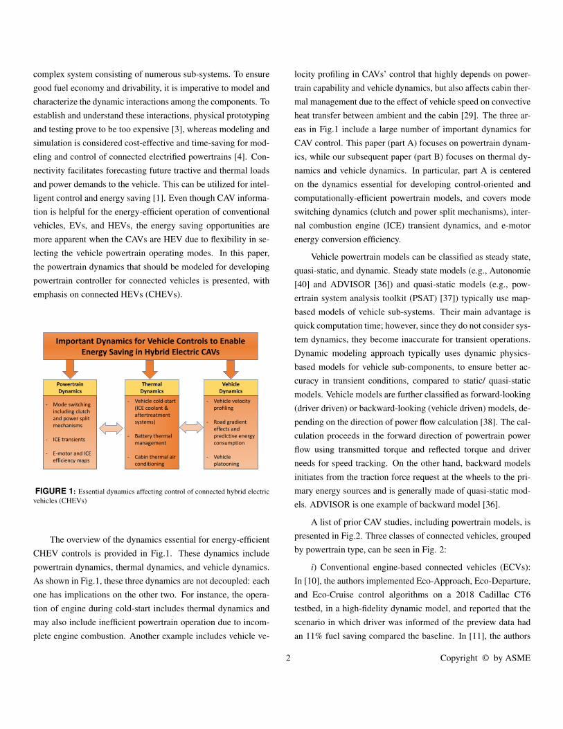
FIGURE 1: Essential dynamics affecting control of connected hybrid electric

vehicles (CHEVs)

The overview of the dynamics essential for energy-efficient

CHEV controls is provided in Fig.1. These dynamics include

powertrain dynamics, thermal dynamics, and vehicle dynamics.

As shown in Fig.1, these three dynamics are not decoupled: each

one has implications on the other two. For instance, the opera-

tion of engine during cold-start includes thermal dynamics and

may also include inefficient powertrain operation due to incom-

plete engine combustion. Another example includes vehicle ve-

locity profiling in CAVs’ control that highly depends on power-

train capability and vehicle dynamics, but also affects cabin ther-

mal management due to the effect of vehicle speed on convective

heat transfer between ambient and the cabin [29]. The three ar-

eas in Fig.1 include a large number of important dynamics for

CAV control. This paper (part A) focuses on powertrain dynam-

ics, while our subsequent paper (part B) focuses on thermal dy-

namics and vehicle dynamics. In particular, part A is centered

on the dynamics essential for developing control-oriented and

computationally-efficient powertrain models, and covers mode

switching dynamics (clutch and power split mechanisms), inter-

nal combustion engine (ICE) transient dynamics, and e-motor

energy conversion efficiency.

Vehicle powertrain models can be classified as steady state,

quasi-static, and dynamic. Steady state models (e.g., Autonomie

[40] and ADVISOR [36]) and quasi-static models (e.g., pow-

ertrain system analysis toolkit (PSAT) [37]) typically use map-

based models of vehicle sub-systems. Their main advantage is

quick computation time; however, since they do not consider sys-

tem dynamics, they become inaccurate for transient operations.

Dynamic modeling approach typically uses dynamic physics-

based models for vehicle sub-components, to ensure better ac-

curacy in transient conditions, compared to static/ quasi-static

models. Vehicle models are further classified as forward-looking

(driver driven) or backward-looking (vehicle driven) models, de-

pending on the direction of power flow calculation [38]. The cal-

culation proceeds in the forward direction of powertrain power

flow using transmitted torque and reflected torque and driver

needs for speed tracking. On the other hand, backward models

initiates from the traction force request at the wheels to the pri-

mary energy sources and is generally made of quasi-static mod-

els. ADVISOR is one example of backward model [36].

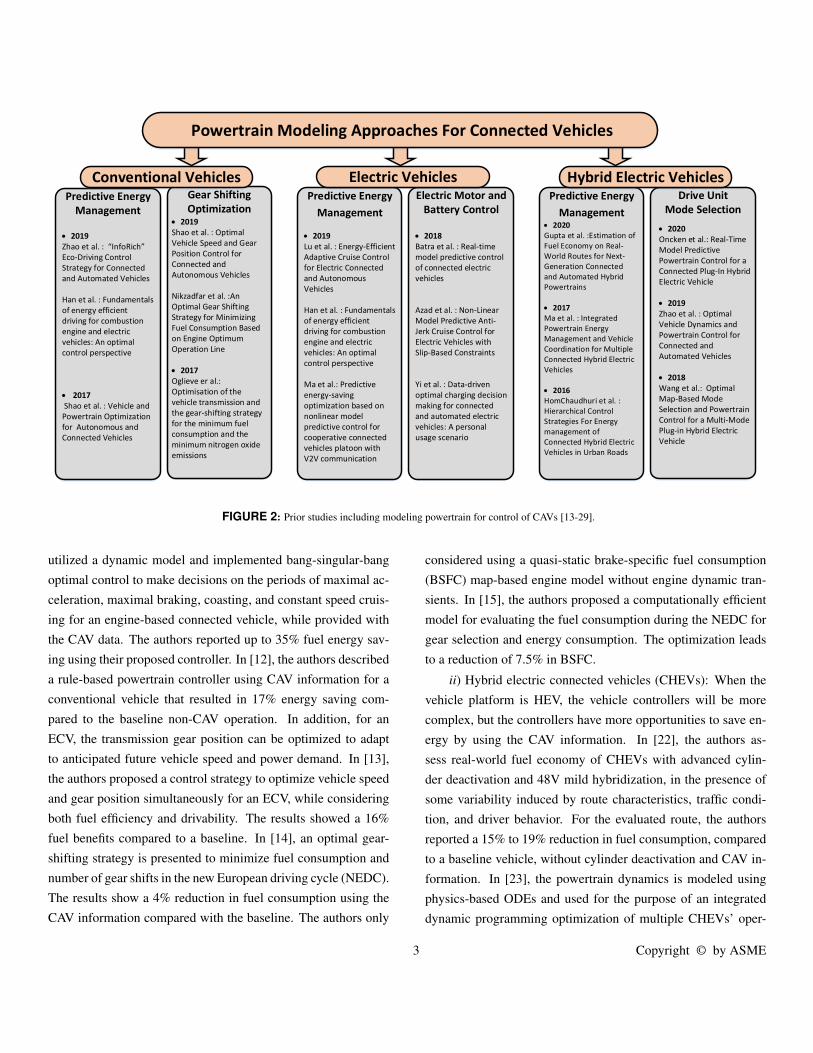
A list of prior CAV studies, including powertrain models, is

presented in Fig.2. Three classes of connected vehicles, grouped

by powertrain type, can be seen in Fig. 2:

i) Conventional engine-based connected vehicles (ECVs):

In [10], the authors implemented Eco-Approach, Eco-Departure,

and Eco-Cruise control algorithms on a 2018 Cadillac CT6

testbed, in a high-fidelity dynamic model, and reported that the

scenario in which driver was informed of the preview data had

an 11% fuel saving compared the baseline. In [11], the authors


Gear Shifting

OptimizationPredictive Energy

Management

• 2019

Zhao et al. : “InfoRich” Eco-Driving Control

Strategy for Connected

and Automated Vehicles

Han et al. : Fundamentals

of energy efficient

driving for combustion

engine and electric

vehicles: An optimal

control perspective

• 2017

Shao et al. : Vehicle and

Powertrain Optimization

for Autonomous and

Connected Vehicles

• 2019

Shao et al. : Optimal

Vehicle Speed and Gear

Position Control for

Connected and

Autonomous Vehicles

Nikzadfar et al. :An

Optimal Gear Shifting

Strategy for Minimizing

Fuel Consumption Based

on Engine Optimum

Operation Line

• 2017

Oglieve er al.:

Optimisation of the

vehicle transmission and

the gear-shifting strategy

for the minimum fuel

consumption and the

minimum nitrogen oxide

emissions

Predictive Energy

Management

Electric Motor and

Battery Control

Conventional Vehicles

Powertrain Modeling Approaches For Connected Vehicles

Predictive Energy

Management

Drive Unit

Mode Selection

• 2019

Lu et al. : Energy-Efficient

Adaptive Cruise Control

for Electric Connected

and Autonomous

Vehicles

Han et al. : Fundamentals

of energy efficient

driving for combustion

engine and electric

vehicles: An optimal

control perspective

Ma et al.: Predictive

energy-saving

optimization based on

nonlinear model

predictive control for

cooperative connected

vehicles platoon with

V2V communication

• 2018

Batra et al. : Real-time

model predictive control

of connected electric

vehicles

Azad et al. : Non-Linear

Model Predictive Anti-

Jerk Cruise Control for

Electric Vehicles with

Slip-Based Constraints

Yi et al. : Data-driven

optimal charging decision

making for connected

and automated electric

vehicles: A personal

usage scenario

• 2020

Gupta et al. :Estimation of

Fuel Economy on Real-

World Routes for Next-

Generation Connected

and Automated Hybrid

Powertrains

• 2017

Ma et al. : Integrated

Powertrain Energy

Management and Vehicle

Coordination for Multiple

Connected Hybrid Electric

Vehicles

• 2016

HomChaudhuri et al. :

Hierarchical Control

Strategies For Energy

management of

Connected Hybrid Electric

Vehicles in Urban Roads

• 2020

Oncken et al.: Real-Time

Model Predictive

Powertrain Control for a

Connected Plug-In Hybrid

Electric Vehicle

• 2019

Zhao et al. : Optimal

Vehicle Dynamics and

Powertrain Control for

Connected and

Automated Vehicles

• 2018

Wang et al.: Optimal

Map-Based Mode

Selection and Powertrain

Control for a Multi-Mode

Plug-in Hybrid Electric

Vehicle

Electric Vehicles Hybrid Electric Vehicles

FIGURE 2: Prior studies including modeling powertrain for control of CAVs [13-29].

utilized a dynamic model and implemented bang-singular-bang

optimal control to make decisions on the periods of maximal ac-

celeration, maximal braking, coasting, and constant speed cruis-

ing for an engine-based connected vehicle, while provided with

the CAV data. The authors reported up to 35% fuel energy sav-

ing using their proposed controller. In [12], the authors described

a rule-based powertrain controller using CAV information for a

conventional vehicle that resulted in 17% energy saving com-

pared to the baseline non-CAV operation. In addition, for an

ECV, the transmission gear position can be optimized to adapt

to anticipated future vehicle speed and power demand. In [13],

the authors proposed a control strategy to optimize vehicle speed

and gear position simultaneously for an ECV, while considering

both fuel efficiency and drivability. The results showed a 16%

fuel benefits compared to a baseline. In [14], an optimal gear-

shifting strategy is presented to minimize fuel consumption and

number of gear shifts in the new European driving cycle (NEDC).

The results show a 4% reduction in fuel consumption using the

CAV information compared with the baseline. The authors only

considered using a quasi-static brake-specific fuel consumption

(BSFC) map-based engine model without engine dynamic tran-

sients. In [15], the authors proposed a computationally efficient

model for evaluating the fuel consumption during the NEDC for

gear selection and energy consumption. The optimization leads

to a reduction of 7.5% in BSFC.

ii) Hybrid electric connected vehicles (CHEVs): When the

vehicle platform is HEV, the vehicle controllers will be more

complex, but the controllers have more opportunities to save en-

ergy by using the CAV information. In [22], the authors as-

sess real-world fuel economy of CHEVs with advanced cylin-

der deactivation and 48V mild hybridization, in the presence of

some variability induced by route characteristics, traffic condi-

tion, and driver behavior. For the evaluated route, the authors

reported a 15% to 19% reduction in fuel consumption, compared

to a baseline vehicle, without cylinder deactivation and CAV in-

formation. In [23], the powertrain dynamics is modeled using

physics-based ODEs and used for the purpose of an integrated

dynamic programming optimization of multiple CHEVs’ oper-


ation, to achieve group-level energy efficiency. In [24], the au-

thors present a fuel efficient and hierarchical Model Predictive

Control (MPC) strategy based on Equivalent Consumption Min-

imization strategy (ECMS) for a group of CHEVs in urban road

conditions, and report an overall 12% energy consumption reduc-

tion compared with the baseline. In [26], the authors presented a

two-level control architecture for a CHEV to optimize the vehi-

cle speed profile and powertrain efficiency simultaneously. The

powertrain is modeled in Vehicle-Engine SIMulation (VESIM)

environment, whereas VISSIM is also used for traffic modeling.

Improvements of fuel efficiency compared with the baseline sce-

narios, under different traffic conditions, range from 7% to 40%.

In [27], the authors present an optimal map-based mode selection

and powertrain control for a multi-mode CHEV. The best mode

map and the best operation maps for powertrain components are

generated using ECMS to minimize equivalent fuel cost at each

operating point. In [28], the authors studied a drive mode op-

timization problem on a Chevrolet Volt to enable optimal drive

modes for fuel minimization based on trip information, using a

multidimensional correlation powertrain model.

iii) Fully-electric connected vehicles (CEVs): In [17], the

authors developed a map-based EV powertrain model to explore

the effects of different velocity profiling methods on energy effi-

ciency of simulated CEVs in a single-lane traffic stream. In [11],

the authors used a simplified EV model to explore the effect of

different control strategies on the energy consumption. In [18],

the authors simulate rear wheel CEVs driven by two permanent

magnet synchronous in-wheel motors (PMSM), and reported en-

ergy savings up to 6% for Urban Dynamometer Driving Schedule

(UDDS) obtained through proposed control algorithms. In [19],

a look-ahead model predictive controller (LA-MPC) is designed

that calculates the required motor torque demand to meet the

dual objectives of increased traction, and anti-jerk control of a

CEV. The authors developed a high-fidelity powertrain model

in MapleSim software, and then reduced the order of the model

for real-time control. In [20], the authors developed a nonlinear

model predictive (NMPC) low-jerk cruise controller for an elec-

tric vehicle. A high-fidelity longitudinal dynamics model was

developed for the test vehicle. The performance of the controller

on the jerk index of the vehicle was assessed in a HIL simulation

using the high-fidelity vehicle model while following a US06

driving cycle. In [21], the authors utilized a correlation-based

powertrain model to perform a dynamic programming optimiza-

tion for charging decisions of a CEV.

This paper builds upon our extensive study for CHEV mod-

eling and control as part of the U.S Department of Energy

ARPA-e NEXTCAR program. The main new contributions of

this work are: i) presenting the essential dynamics, includ-

ing the engine transients and operating mode switching energy

penalties, needed for computationally efficient and real-time

control-oriented powertrain modeling of a CHEV, ii) system-

atic low-order modeling and experimental validation of power-

train dynamics suitable for fast execution with low computa-

tional cost, iii) vehicle experimentation and characterization at

the component-level and system-level for charge-depleting and

charge-sustaining operating modes, and iv) assessment of energy

distribution of the test vehicle by sub-component in the charge-

depleting operation mode for three U.S drive cycles. It is note-

worthy that in none of the studies mentioned previously, the au-

thors explicitly stated that they have used engine fuel penalty

terms in powertrain modeling.

The structure of this paper is as follows: in Section 2, the ve-

hicle setup, instrumented sensor suites, and the CAN-based data

acquisition procedure is discussed. In Section 3, the powertrain

dynamics and the experimental model validation of various pow-

ertrain sub-systems are discussed. After each sub-system model

description, validation of that sub-system for the US06 drive cy-

cle is followed. Included in this Section are engine transient dy-

namic model, engine fuel penalty terms, mode switching energy

penalty terms, modeling of e-motor, drive unit, and Li-ion bat-

tery. Section 4 investigates: i) interdependence of the powertrain

operating mode and the efficiency ii) energy distribution anal-

ysis of the test vehicle at the sub-component level, and iii) the

effect of hysteresis on the powertrain dynamics and efficiency.

Section 5 summarizes the findings from this paper.

2 Vehicle Test Setup

The test vehicle of this study is a Chevy Volt II generation,

a light-duty plug-in HEV with two motor-generator units and an

engine for propulsion. The test vehicle could be run in pure elec-

tric, hybrid electric, and conventional engine operations. This al-

lows to determine vehicle powertrain dynamics for varying elec-


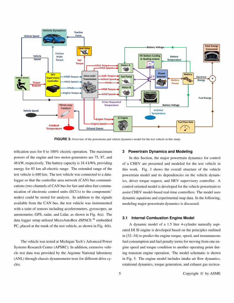
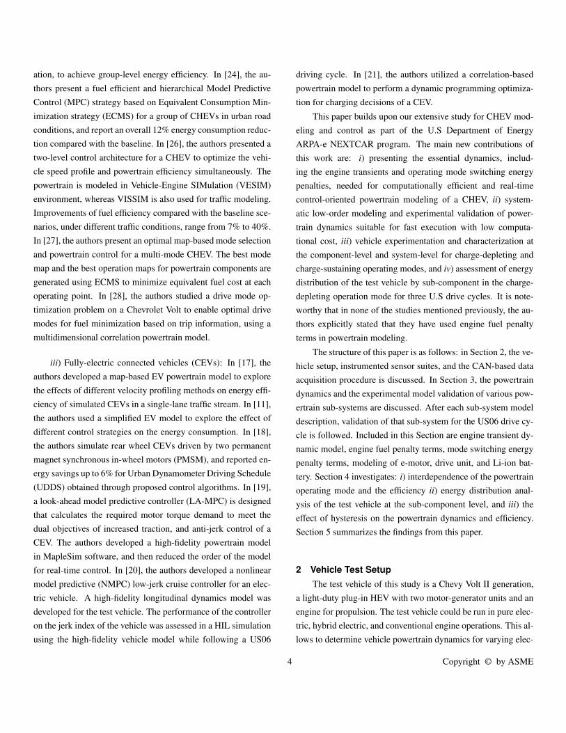
FIGURE 3: Overview of the powertrain and vehicle dynamics model for the test vehicle in this study.

trification uses for 0 to 100% electric operation. The maximum

powers of the engine and two motor-generators are 75, 87, and

48 kW, respectively. The battery capacity is 18.4 kWh, providing

energy for 85 km all-electric range. The extended range of the

test vehicle is 680 km. The test vehicle was connected to a data-

logger so that the controller area network (CAN) bus communi-

cations (two channels of CAN bus for fast and ultra-fast commu-

nication of electronic control units (ECUs) to the components’

nodes) could be stored for analysis. In addition to the signals

available from the CAN bus, the test vehicle was instrumented

with a suite of sensors including accelerometers, gyroscopes, an

anemometer, GPS, radar, and Lidar, as shown in Fig. 4(a). The

data logger setup utilized MicroAutoBox dSPACE ® embedded

PC, placed at the trunk of the test vehicle, as shown in Fig. 4(b).

The vehicle was tested at Michigan Tech’s Advanced Power

Systems Research Center (APSRC). In addition, extensive vehi-

cle test data was provided by the Argonne National laboratory

(ANL) through chassis dynamometer tests for different drive cy-

cles.

3 Powertrain Dynamics and Modeling

In this Section, the major powertrain dynamics for control

of a CHEV are presented and modeled for the test vehicle in

this work. Fig. 3 shows the overall structure of the vehicle

powertrain model and its dependencies on the vehicle dynam-

ics, driver torque request, and HEV supervisory controller. A

control-oriented model is developed for the vehicle powertrain to

assist CHEV model-based real-time controllers. The model uses

dynamic equations and experimental map data. In the following,

modeling major powertrain dynamics is discussed.

3.1 Internal Combustion Engine Model

A dynamic model of a 1.5 liter 4-cylinder naturally aspi-

rated DI SI engine is developed based on the principles outlined

in [32–34] to predict the engine torque, speed, and instantaneous

fuel consumption and fuel penalty terms for moving from one en-

gine speed and torque condition to another operating point dur-

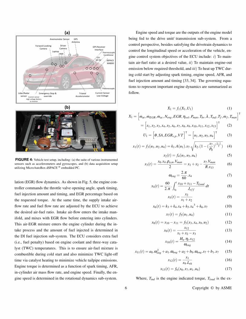
ing transient engine operation. The model schematic is shown

in Fig. 5. The engine model includes intake air flow dynamics,

rotational dynamics, torque generation, and exhaust gas recircu-


(a)

(b)

Lidar/Radar

sensor Current sensor

High voltage Battery

to Inverter

Emergency Stop &

override

Triaxial

Accelerometer

Current Sensor

Low Voltage

Thermocouple

Forward Looking

Camera

GPS

Antenna

Anemometer Sensor

Driver

Camera

LaptopHMI

dSPACE

MABXII

GPS Receiver

Interface

Thermocouple

Conditioner

12V

DC-DC

FIGURE 4: Vehicle test setup, including: (a) the suite of various instrumented

sensors such as accelerometers and gyroscopes, and (b) data acquisition setup

utilizing MicroAutoBox dSPACE ® embedded PC.

lation (EGR) flow dynamics. As shown in Fig. 5, the engine con-

troller commands the throttle valve opening angle, spark timing,

fuel injection amount and timing, and EGR percentage based on

the requested torque. At the same time, the supply intake air-

flow rate and fuel flow rate are adjusted by the ECU to achieve

the desired air-fuel ratio. Intake air-flow enters the intake man-

ifold, and mixes with EGR flow before entering into cylinders.

This air-EGR mixture enters the engine cylinder during the in-

take process and the amount of fuel injected is determined in

the DI fuel injection sub-system. The ECU considers extra fuel

(i.e., fuel penalty) based on engine coolant and three-way cata-

lyst (TWC) temperatures. This is to ensure air-fuel mixture is

combustible during cold start and also minimize TWC light-off

time via catalyst heating to minimize vehicle tailpipe emissions.

Engine torque is determined as a function of spark timing, AFR,

in-cylinder air mass flow rate, and engine speed. Finally, the en-

gine speed is determined in the rotational dynamics sub-system.

Engine speed and torque are the outputs of the engine model

being fed to the drive unit/ transmission sub-system. From a

control perspective, besides satisfying the drivetrain dynamics to

control the longitudinal speed or acceleration of the vehicle, en-

gine control system objectives of the ECU include: i) To main-

tain air-fuel ratio at a desired value, ii) To maintain engine-out

emission below required threshold, and iii) To heat up TWC dur-

ing cold start by adjusting spark timing, engine speed, AFR, and

fuel injection amount and timing [33, 34]. The governing equa-

tions to represent important engine dynamics are summarized as

follow.

X1 = f1(X1,U1) (1)

X1 =[

mat , mEGR, mac,Neng,EGR,ηvol ,Pman,Tbr,λ ,Tind ,Tf , m f ,Tman

]

⊺

=[

x1,x2,x3,x4,x5,x6,x7,x8,x9,x10,x11,x12,x13

]

⊺

(2)

U1 =[

θ ,SA,EGRv,p,V T

]

⊺

=[

u1,u2,u3,u4

]

⊺

(3)

x1(t) = f3(u1,u2,u4) = k1.A(u1).x7.

√

k2.(1− (x7

P0)(

γ−1γ ) (4)

x2(t) = f4(u1,u3,u4) (5)

x3(t) =x6.x4.ρa,m.Vman

2= x1 + x2 −

x7.Vman

R.x13(6)

ωeng =2.π

60.x4 (7)

x4(t) =60

2.π.∫ t

t0

x10 + x11 −TLoad

Je f f

dt (8)

x5(t) =x2

x1 + x2(9)

x6(t) = k3 + k4.x4 + k5.x43 + k6.x7 (10)

x7(t) = f5(u1,u4) (11)

x8(t) = x10 − x11 = f5(x3,x4,x9,u2) (12)

x9(t) =x12

x1 + x2 − x3(13)

x10(t) =Hu.ηi.x12

ωeng

(14)

x11(t) = a0.ω2eng +a1.ωeng +a2 +b0.ωeng.x7 +b1.x7 (15)

x12(t) =x1

x9.Lth

(16)

x13(t) = f6(x6,x7,u1,u4) (17)

Where, Tind is the engine indicated torque, Tload is the ex-


FIGURE 5: The developed engine dynamic model in this study.

ternal load torque on the crankshaft, Tf represents the pumping

and friction losses in the engine and Je f f is the effective rota-

tional moment of inertia for the engine crankshaft, SA is spark

advance, EGRv,p is the valve position for EGR, V T is the valve

timing command from the ECU, Hu is the heating value of fuel,

ηi is the indicated thermal efficiency. m f represents the fuel mass

flow rate into the cylinders.

Lth is the stoichiometric air/fuel mass ratio for gasoline fuel

and λ is the air/fuel equivalence ratio. The term Tf represents the

hydrodynamic and pumping friction losses represented in terms

of a loss torque. Hydrodynamic or fluid-film friction is the prin-

cipal component of mechanical friction losses in the engine [34].

a0, a1, a2, b0, and b1 are parameters that are determined

by experimental engine testing to calculate the friction torque.

θ is the throttle angle, A(u1) = A(θ)= AT is the throttle angle-

dependent area, mat is the throttle air flow rate, mEGR is the EGR

flow rate, mac is the in–cylinder air flow rate, Vman is the intake

manifold volume, Tman is the manifold temperature, Ru is the uni-

versal gas constant, ηvol is the volumetric efficiency, ρa,m is the

air density, N is the engine speed, k1 = CD.γ0.5

√R.T0

, k2 = 2×γγ−1

, and

K3, K4, K5, and K6 are regression constants. CD is the discharge

coefficient of valves, P0 and T0 are the ambient pressure and tem-

perature values, respectively, ωeng is the angular speed of engine

crankshaft in rad/sec, Tbr is the engine brake troque (N.m), pr is

ratio of intake manifold pressure to ambient pressure, and γ is

specific heat ratio. Volumetric efficiency (ηvol) depends on the

manifold pressure and the engine speed, and is estimated using

regression of experimental engine data.

3.1.1 Engine Startup Fuel Penalty Engine and

three-way catalyst (TWC) thermal conditions and temperatures

play important roles in ECU strategies to adjust fuel injections.

These affect the engine fuel flow rate and should be considered


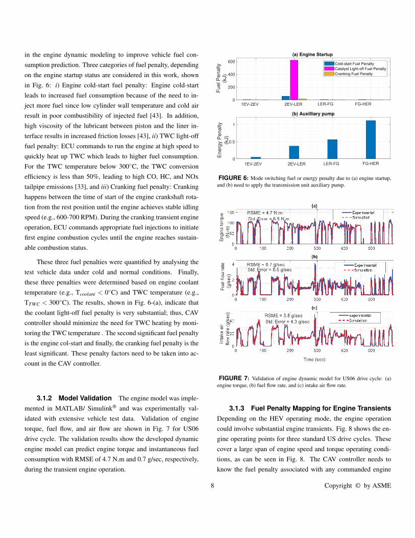
in the engine dynamic modeling to improve vehicle fuel con-

sumption prediction. Three categories of fuel penalty, depending

on the engine startup status are considered in this work, shown

in Fig. 6: i) Engine cold-start fuel penalty: Engine cold-start

leads to increased fuel consumption because of the need to in-

ject more fuel since low cylinder wall temperature and cold air

result in poor combustibility of injected fuel [43]. In addition,

high viscosity of the lubricant between piston and the liner in-

terface results in increased friction losses [43], ii) TWC light-off

fuel penalty: ECU commands to run the engine at high speed to

quickly heat up TWC which leads to higher fuel consumption.

For the TWC temperature below 300C, the TWC conversion

efficiency is less than 50%, leading to high CO, HC, and NOx

tailpipe emissions [33], and iii) Cranking fuel penalty: Cranking

happens between the time of start of the engine crankshaft rota-

tion from the rest position until the engine achieves stable idling

speed (e.g., 600-700 RPM). During the cranking transient engine

operation, ECU commands appropriate fuel injections to initiate

first engine combustion cycles until the engine reaches sustain-

able combustion status.

These three fuel penalties were quantified by analysing the

test vehicle data under cold and normal conditions. Finally,

these three penalties were determined based on engine coolant

temperature (e.g., Tcoolant < 0C) and TWC temperature (e.g.,

TTWC < 300C). The results, shown in Fig. 6-(a), indicate that

the coolant light-off fuel penalty is very substantial; thus, CAV

controller should minimize the need for TWC heating by moni-

toring the TWC temperature . The second significant fuel penalty

is the engine col-start and finally, the cranking fuel penalty is the

least significant. These penalty factors need to be taken into ac-

count in the CAV controller.

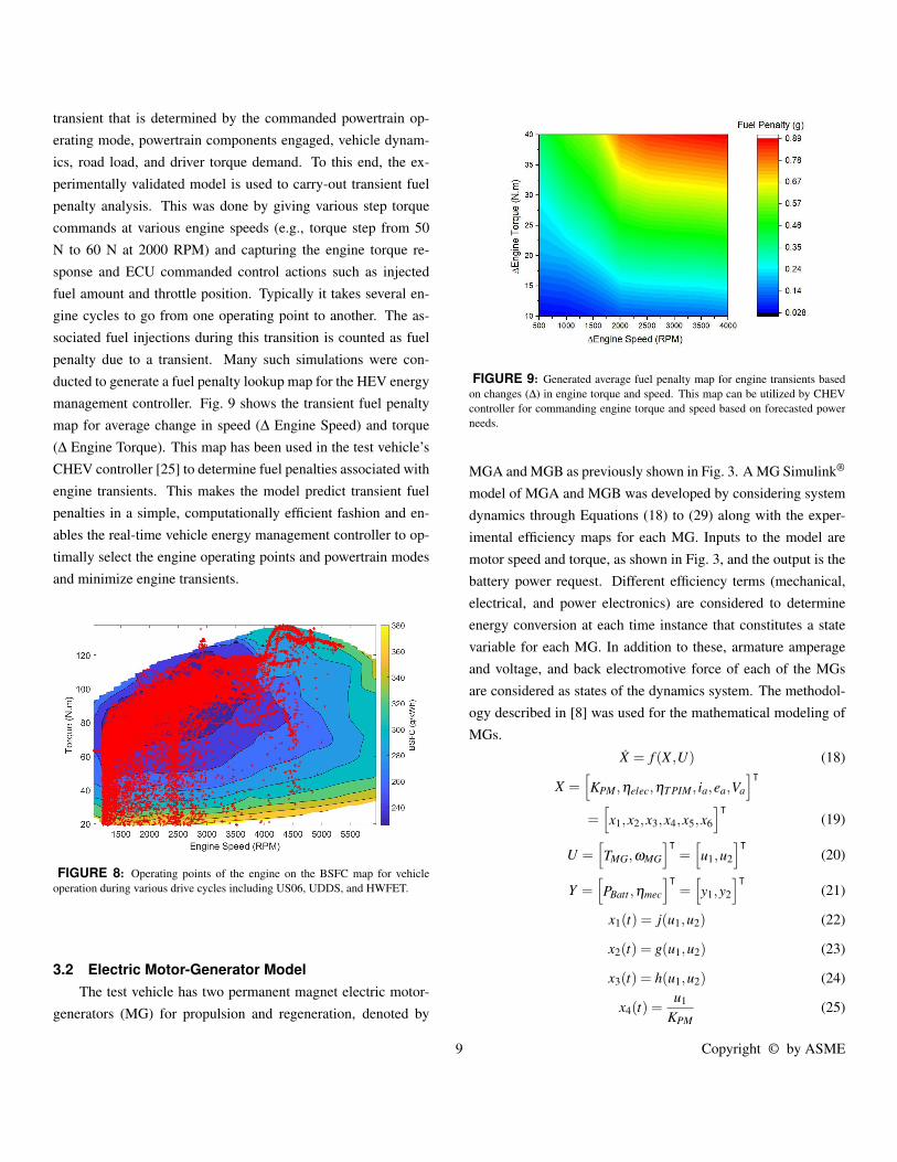
3.1.2 Model Validation The engine model was imple-

mented in MATLAB/ Simulink® and was experimentally val-

idated with extensive vehicle test data. Validation of engine

torque, fuel flow, and air flow are shown in Fig. 7 for US06

drive cycle. The validation results show the developed dynamic

engine model can predict engine torque and instantaneous fuel

consumption with RMSE of 4.7 N.m and 0.7 g/sec, respectively,

during the transient engine operation.

(a) Engine Startup

1EV-2EV 2EV-LER LER-FG FG-HER0

200

400

600

Fuel P

enalty

(kJ)

Cold-start Fuel Penalty

Catalyst Light-off Fuel Penalty

Cranking Fuel Penalty

(b) Auxilliary pump

0

0.5

1

Energ

y P

enalty

(kJ)

1EV-2EV 2EV-LER LER-FG FG-HER

FIGURE 6: Mode switching fuel or energy penalty due to (a) engine startup,

and (b) need to apply the transmission unit auxiliary pump.

FIGURE 7: Validation of engine dynamic model for US06 drive cycle: (a)

engine torque, (b) fuel flow rate, and (c) intake air flow rate.

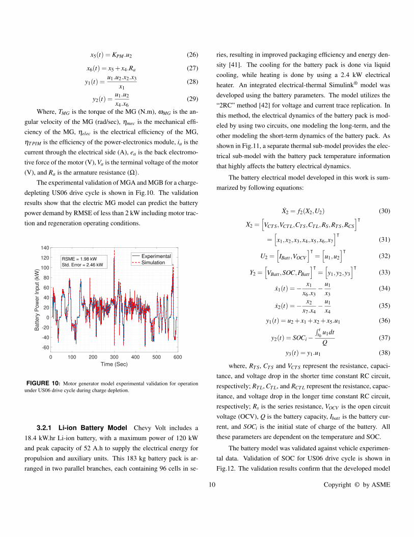
3.1.3 Fuel Penalty Mapping for Engine Transients

Depending on the HEV operating mode, the engine operation

could involve substantial engine transients. Fig. 8 shows the en-

gine operating points for three standard US drive cycles. These

cover a large span of engine speed and torque operating condi-

tions, as can be seen in Fig. 8. The CAV controller needs to

know the fuel penalty associated with any commanded engine


transient that is determined by the commanded powertrain op-

erating mode, powertrain components engaged, vehicle dynam-

ics, road load, and driver torque demand. To this end, the ex-

perimentally validated model is used to carry-out transient fuel

penalty analysis. This was done by giving various step torque

commands at various engine speeds (e.g., torque step from 50

N to 60 N at 2000 RPM) and capturing the engine torque re-

sponse and ECU commanded control actions such as injected

fuel amount and throttle position. Typically it takes several en-

gine cycles to go from one operating point to another. The as-

sociated fuel injections during this transition is counted as fuel

penalty due to a transient. Many such simulations were con-

ducted to generate a fuel penalty lookup map for the HEV energy

management controller. Fig. 9 shows the transient fuel penalty

map for average change in speed (∆ Engine Speed) and torque

(∆ Engine Torque). This map has been used in the test vehicle’s

CHEV controller [25] to determine fuel penalties associated with

engine transients. This makes the model predict transient fuel

penalties in a simple, computationally efficient fashion and en-

ables the real-time vehicle energy management controller to op-

timally select the engine operating points and powertrain modes

and minimize engine transients.

FIGURE 8: Operating points of the engine on the BSFC map for vehicle

operation during various drive cycles including US06, UDDS, and HWFET.

3.2 Electric Motor-Generator Model

The test vehicle has two permanent magnet electric motor-

generators (MG) for propulsion and regeneration, denoted by

FIGURE 9: Generated average fuel penalty map for engine transients based

on changes (∆) in engine torque and speed. This map can be utilized by CHEV

controller for commanding engine torque and speed based on forecasted power

needs.

MGA and MGB as previously shown in Fig. 3. A MG Simulink®

model of MGA and MGB was developed by considering system

dynamics through Equations (18) to (29) along with the exper-

imental efficiency maps for each MG. Inputs to the model are

motor speed and torque, as shown in Fig. 3, and the output is the

battery power request. Different efficiency terms (mechanical,

electrical, and power electronics) are considered to determine

energy conversion at each time instance that constitutes a state

variable for each MG. In addition to these, armature amperage

and voltage, and back electromotive force of each of the MGs

are considered as states of the dynamics system. The methodol-

ogy described in [8] was used for the mathematical modeling of

MGs.

X = f (X ,U) (18)

X =[

KPM,ηelec,ηT PIM, ia,ea,Va

]

⊺

=[

x1,x2,x3,x4,x5,x6

]

⊺

(19)

U =[

TMG,ωMG

]

⊺

=[

u1,u2

]

⊺

(20)

Y =[

PBatt ,ηmec

]

⊺

=[

y1,y2

]

⊺

(21)

x1(t) = j(u1,u2) (22)

x2(t) = g(u1,u2) (23)

x3(t) = h(u1,u2) (24)

x4(t) =u1

KPM

(25)


x5(t) = KPM.u2 (26)

x6(t) = x5 + x4.Ra (27)

y1(t) =u1.u2.x2.x3

x1(28)

y2(t) =u1.u2

x4.x6

(29)

Where, TMG is the torque of the MG (N.m), ωMG is the an-

gular velocity of the MG (rad/sec), ηmec is the mechanical effi-

ciency of the MG, ηelec is the electrical efficiency of the MG,

ηT PIM is the efficiency of the power-electronics module, ia is the

current through the electrical side (A), ea is the back electromo-

tive force of the motor (V), Va is the terminal voltage of the motor

(V), and Ra is the armature resistance (Ω).

The experimental validation of MGA and MGB for a charge-

depleting US06 drive cycle is shown in Fig.10. The validation

results show that the electric MG model can predict the battery

power demand by RMSE of less than 2 kW including motor trac-

tion and regeneration operating conditions.

0 100 200 300 400 500 600

Time (Sec)

-60

-40

-20

0

20

40

60

80

100

120

140

Battery

Pow

er

Input (k

W)

Experimental

SimulationRSME = 1.98 kW

Std. Error = 2.46 kW

FIGURE 10: Motor generator model experimental validation for operation

under US06 drive cycle during charge depletion.

3.2.1 Li-ion Battery Model Chevy Volt includes a

18.4 kW.hr Li-ion battery, with a maximum power of 120 kW

and peak capacity of 52 A.h to supply the electrical energy for

propulsion and auxiliary units. This 183 kg battery pack is ar-

ranged in two parallel branches, each containing 96 cells in se-

ries, resulting in improved packaging efficiency and energy den-

sity [41]. The cooling for the battery pack is done via liquid

cooling, while heating is done by using a 2.4 kW electrical

heater. An integrated electrical-thermal Simulink® model was

developed using the battery parameters. The model utilizes the

“2RC” method [42] for voltage and current trace replication. In

this method, the electrical dynamics of the battery pack is mod-

eled by using two circuits, one modeling the long-term, and the

other modeling the short-term dynamics of the battery pack. As

shown in Fig.11, a separate thermal sub-model provides the elec-

trical sub-model with the battery pack temperature information

that highly affects the battery electrical dynamics.

The battery electrical model developed in this work is sum-

marized by following equations:

X2 = f2(X2,U2) (30)

X2 =[

VCT S,VCT L,CT S,CT L,RS,RT S,RCS

]

⊺

=[

x1,x2,x3,x4,x5,x6,x7

]

⊺

(31)

U2 =[

IBatt ,VOCV

]

⊺

=[

u1,u2

]

⊺

(32)

Y2 =[

VBatt ,SOC,PBatt

]

⊺

=[

y1,y2,y3

]

⊺

(33)

x1(t) =−x1

x6.x3−

u1

x3(34)

x2(t) =−x2

x7.x4−

u1

x4(35)

y1(t) = u2 + x1 + x2 + x5.u1 (36)

y2(t) = SOCi −

∫ tt0

u1dt

Q(37)

y3(t) = y1.u1 (38)

where, RT S, CT S and VCT S represent the resistance, capaci-

tance, and voltage drop in the shorter time constant RC circuit,

respectively; RT L, CT L, and RCT L represent the resistance, capac-

itance, and voltage drop in the longer time constant RC circuit,

respectively; Rs is the series resistance, VOCV is the open circuit

voltage (OCV), Q is the battery capacity, Ibatt is the battery cur-

rent, and SOCi is the initial state of charge of the battery. All

these parameters are dependent on the temperature and SOC.

The battery model was validated against vehicle experimen-

tal data. Validation of SOC for US06 drive cycle is shown in

Fig.12. The validation results confirm that the developed model


Battery

Heater

TPIM

Battery Thermal Model

Shorter Time

Constant

Longer Time

Constant

Battery Voltage

Battery SOC

`

Voltage

Ambient

Temperature

Battery

Temperature

Ba

tte

ry

Cu

rre

nt

Battery Current

Battery

Temperature

SOC

SOC

SOC

VCTS

VCTL

Battery Current

Battery

Temperature

SOC

`

Current

Heater

Power

FIGURE 11: Developed battery pack model of the test vehicle. TPIM stands

for traction power inverter module.

can estimate SOC with RMSE of less than 0.4 %.

Other methods of battery modeling such as online cell pa-

rameter estimation [45] or recursive neural networks [45] can

be used to improve model accuracy and manage aging, however

these methods need extensive sensor instrumentation inside the

battery pack, or large operating data sets.

100 200 300 400 500 600

Time (sec)

78

80

82

84

86

88

SO

C (

%)

Simulation

Experimental

RMSE = 0.36 %

Std. Error = 0.43 %

FIGURE 12: Battery model experimental validation for predicting SOC dur-

ing charge depleting operation in US06 drive cycle.

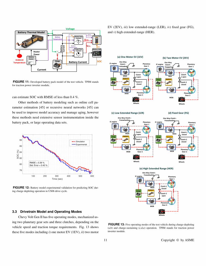
3.3 Drivetrain Model and Operating Modes

Chevy Volt Gen II has five operating modes, mechanized us-

ing two planetary gear sets and three clutches, depending on the

vehicle speed and traction torque requirements. Fig. 13 shows

these five modes including i) one motor EV (1EV), ii) two motor

EV (2EV), iii) low extended-range (LER), iv) fixed gear (FG),

and v) high extended-range (HER).

One Way

Clutch :

Unloaded

Planetary

Gear 1

Planetary

Gear 2

Wheels

Clutch 2

closed

Clutch

1 open

IC engine

TPIMBattery

MGB

MGA

(a) One Motor EV (1EV)

One Way

Clutch :

Engaged

TPIM Battery

MGA

(b) Two Motor EV (2EV)

(c) Low Extended Range (LER) (d) Fixed Gear (FG)

One Way Clutch :

Freewheeling

Clutch 2

closed

Clutch

1 open

TPIM Battery

One Way Clutch :

Freewheeling

Clutch 2

closed

Clutch 1

closed

TPIM Battery

(e) High Extended Range (HER)

One Way Clutch :

Freewheeling

Clutch 2

open

Clutch 1

closed

TPIMBattery

Planetary

Gear 1

Planetary

Gear 2

Wheels

Clutch 2

closed

Clutch

1 open

IC engine

MGB

Planetary

Gear 1

Planetary

Gear 2

Wheels

IC engine

MGB

MGA

Planetary

Gear 1

Planetary

Gear 2

Wheels

IC engine

MGB

MGA

Planetary

Gear 1

Planetary

Gear 2

Wheels

IC engine

MGB

MGA

FIGURE 13: Five operating modes of the test vehicle during charge-depleting

(a,b) and charge-sustaining (c,d,e) operation. TPIM stands for traction power

inverter module.


Fig. 13-(a) shows 1EV mode power flow in which MGB car-

ries out propulsion and regeneration braking. Fig. 13-(b) shows

2EV mode power flow in which both MGB and MGA carry out

propulsion of the vehicle. Fig. 13-(c) shows LER mode power

flow in which the engine assists MGB in vehicle propulsion and

a fraction of engine fuel energy is converted into electrical en-

ergy by MGA. Fig. 13-(d) shows FG mode power flow in which

both engine and MGB propel the vehicle. Fig. 13-(e) shows HER

mode power flow in which engine, MGA, and MGB propel the

vehicle. These modes are decided by the supervisory controller

based on the driver torque request, axle torque, vehicle speed,

battery SOC, acceleration/ deceleration rate, current mode, and

other factors. The equations to capture drivetrain dynamics for

simulating drivetrain output torque and speed can be determined

using the energy balance and kinematics equations. For brevity,

only two sets of these equations for 2EV and HER modes are

mentioned in Eq. (39) and Eq. (40).

Ivehicle 0 0 P1 P2

0 IMGA 0 −S1 0

0 0 IMGB 0 −S2

P1 −S1 0 0 0

P2 0 −S2 0 0

ωout

ωMGA

ωMGB

F1

F2

=

−Tload

TMGA

TMGB

0

0

(39)

Where, IMGA is inertia of MGA. F1 is internal force acting

between the gears of planetary gear 1 (PG1) and, TMGA is torque

generated by MGA. S1 and R1 are radii of sun and ring gear for

planetary gear 1 (PG1). ωMGA is angular acceleration of MGA.

In addition, P1 = S1 +R1 and P2 = S2 +R2.

Ivehicle 0 0 0 P1 P2

0 Ie 0 0 −R1 0

0 0 IMGA 0 −S1 −R2

0 0 0 IMGB 0 −S2

P1 −R1 −S1 0 0 0

P2 0 −P2 0 0

ωout

ωe

ωMGA

ωMGB

F1

F2

=

−Tload

Te

TMGA

TMGB

0

0

(40)

3.4 Mode-switching Energy Penalty

Vehicle components require extra energy to perform mode

transition. If this energy penalty information is known, intelli-

gent strategies can be incorporated in the supervisory controller

to minimize those energy penalties and optimize energy con-

sumption. There is an energy penalty associated with the mode

switching in the test vehicle, depending which modes are in-

volved. For instance, for switching from 2EV to LER mode

requires the engine to start. As explained previously in Sec-

tion 3.1, depending on the engine coolant temperature and TWC

temperature, fuel penalties are induced and should be considered.

Fig. 6-(a) shows the mode switching penalty as a result of engine

startup.

The vehicle transmission unit includes a pump, an auxiliary

pump, and a transmission. The pump pressurizes transmission

oil when an engine is operating; however, when the engine is

not operating, the auxiliary pump coupled to the pump in paral-

lel pressurizes the transmission oil. During mode transitions, the

test data of the test vehicle’s auxiliary pump showed an instant

increase (i.e., spike) in auxiliary pump power consumption for a

few seconds. This spike in power should be considered as part of

the mode switch penalty. A data-driven auxiliary pump model is

developed and validated to estimate the energy consumption by

the auxiliary pump. As shown in Fig. 6-(b), the energy penal-

ties associated with mode switching in transmission unit auxil-

iary pump results in energy penalties over 1 kJ (for FG to HER

mode switch). This is because of the higher vehicle speed and

tractive effort in the HER mode, which tolls the transmission unit

auxiliary pump.

4 Discussion

The developed powertrain model from Section 3 can be used

for analysis, optimization, and design of control strategies for

CHEVs. Examples of the application of the powertrain model

could be: i) selection of optimum vehicle operating mode (1EV,

2EV, LER, FG, HER), ii) selection of optimum speed and torque

for the e-motor and the engine, and iii) design of mode-switching

strategies by considering powertrain energy penalty occurrences

during each mode switching. Here, these applications are briefly

explained.

The powertrain operation and CHEV energy consumption

highly depends on the vehicle mode of operation. Fig. 14 shows

the vehicle speed and operating modes for charge-sustaining op-

eration of the test vehicle during US06, UDDS, and HWFET


drive cycles. It can be seen that the vehicle operates in FG and

HER modes at higher speeds and use LER mode to transition to

the two modes. To start the vehicle from the stationary condition,

the vehicle is commanded to operate in EV1 and EV2 modes by

the supervisory controller. The threshold values for deciding to

operate the vehicle in different modes can be optimally selected

when the transient dynamics of the vehicle is taken into account.

0 100 200 300 400 500 6000

100

Ve

locity (

kp

h)

(a) US061EV 2EV LER FG HER

0 200 400 600 800 1000 12000

50

100

Ve

locity (

kp

h)

(b) UDDS1EV 2EV LER FG HER

0 100 200 300 400 500 600 700

Time (Sec)

0

50

100

Ve

locity (

kp

h)

(c) HWFET

1EV 2EV LER FG HER

FIGURE 14: Vehicle operating modes (Fig. 13) during three US federal drive

cycles.

The developed model from Section 3 is used to analyze pow-

ertrain operation during the three drive cycles in Fig. 14. The re-

sults are shown in Figures 15 to 17. The following observations

can be made: i) The engine operating points for the FG mode

are very well located in the efficient BSFC region; however, for

the LER and HER modes, the distribution of operating points is

scattered across larger BSFC region with poor efficiency values

compared to the FG mode (shown in Fig. 15). The center of LER,

FG, and HER point clusters is: 82 N.m and 2400 RPM for LER

mode, 100 N.m and 3000 RPM for FG mode, and 80 N.m and

1900 RPM for HER mode. This is because all prime movers of

the vehicle being involved at LER and HER modes for propul-

sion, while for the FG mode, the only operating prime mover is

the engine. This results in sub-optimal engine operation in LER

and HER modes at the expense of meeting other requirements for

MGA and MGB, beyond just the engine BSFC efficiency. ii) As

shown in the Fig. 16, the e-motors’ operation in four quadrants of

the speed-torque plane have distinct patterns. MGA is a smaller

and less efficient e-motor compared with MGB (maximum effi-

ciency of 94% vs 96%) and achieves its maximum efficiency at

higher speeds. During the US06 drive cycle, the MGA rarely op-

erates at the best efficiency points and instead, operates with 80%

to 91% efficiency, while MGB operates frequently in its high ef-

ficiency region and overall, operates with 86% to 96% efficiency.

For US06 drive cycle, the average efficiencies of MGA and MGB

are 89.1% and 92.5%, respectively. iii) for quadrant two (posi-

tive torque and negative speed), MGA and MGB only operate

in the LER and HER modes, respectively. The same pattern is

observed for quadrant three (negative torque and speed).

1000 2000 3000 4000 5000 6000

Engine speed (RPM)

20

40

60

80

100

120

En

gin

e t

orq

ue

(N

.m)

240

260

280

300

320

340

360

BS

FC

(g

/kW

h)

BSFC

EV1

EV2

LER

FER

HER

FIGURE 15: Engine operating points on the engine BSFC map along with

vehicle operating modes for US06 drive cycle.

Vehicle operation in the charge depleting mode is analyzed

using the developed powertrain model and part of the results

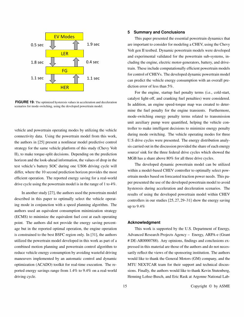
is shown in Fig.17. The results indicate that: i) MGB con-

sumes the majority of the energy in all three drive cycles. Since

the UDDS cycle has frequent start-stop events and low driving

speeds, MGA assists total requirements but its contribution is

about 1% of the total. For the high speed drive cycles of HWFET

and US06, MGA is used negligibly, too. ii) The auxiliary pump

losses are much higher in the UDDS drive cycle at 8% of total


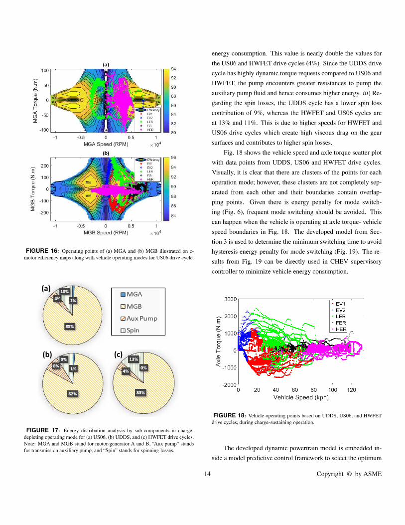
FIGURE 16: Operating points of (a) MGA and (b) MGB illustrated on e-

motor efficiency maps along with vehicle operating modes for US06 drive cycle.

(a)

(b) (c)

FIGURE 17: Energy distribution analysis by sub-components in charge-

depleting operating mode for (a) US06, (b) UDDS, and (c) HWFET drive cycles.

Note: MGA and MGB stand for motor-generator A and B, “Aux pump” stands

for transmission auxiliary pump, and “Spin” stands for spinning losses.

energy consumption. This value is nearly double the values for

the US06 and HWFET drive cycles (4%). Since the UDDS drive

cycle has highly dynamic torque requests compared to US06 and

HWFET, the pump encounters greater resistances to pump the

auxiliary pump fluid and hence consumes higher energy. iii) Re-

garding the spin losses, the UDDS cycle has a lower spin loss

contribution of 9%, whereas the HWFET and US06 cycles are

at 13% and 11%. This is due to higher speeds for HWFET and

US06 drive cycles which create high viscous drag on the gear

surfaces and contributes to higher spin losses.

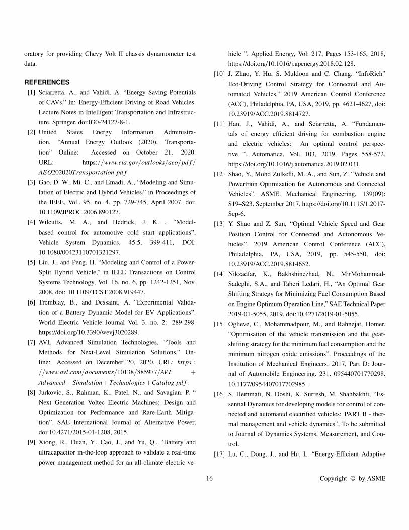
Fig. 18 shows the vehicle speed and axle torque scatter plot

with data points from UDDS, US06 and HWFET drive cycles.

Visually, it is clear that there are clusters of the points for each

operation mode; however, these clusters are not completely sep-

arated from each other and their boundaries contain overlap-

ping points. Given there is energy penalty for mode switch-

ing (Fig. 6), frequent mode switching should be avoided. This

can happen when the vehicle is operating at axle torque- vehicle

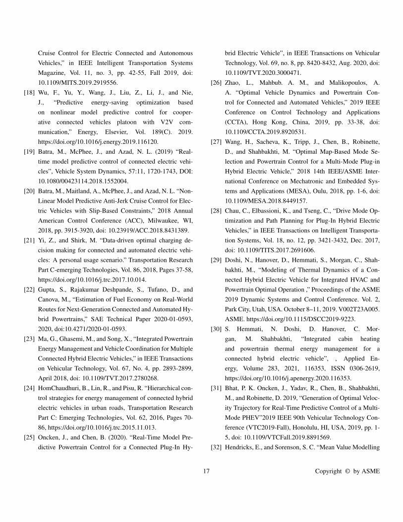
speed boundaries in Fig. 18. The developed model from Sec-

tion 3 is used to determine the minimum switching time to avoid

hysteresis energy penalty for mode switching (Fig. 19). The re-

sults from Fig. 19 can be directly used in CHEV supervisory

controller to minimize vehicle energy consumption.

FIGURE 18: Vehicle operating points based on UDDS, US06, and HWFET

drive cycles, during charge-sustaining operation.

The developed dynamic powertrain model is embedded in-

side a model predictive control framework to select the optimum


LER

0.5 sec

1.8 sec

1.1 sec

1.9 sec

0.4 sec

1.1 sec

FG

HER

EV Modes

FIGURE 19: The optimized hysteresis values in acceleration and deceleration

scenarios for mode-switching, using the developed powertrain model.

vehicle and powertrain operating modes by utilizing the vehicle

connectivity data. Using the powertrain model from this work,

the authors in [25] present a nonlinear model predictive control

strategy for the same vehicle platform of this study (Chevy Volt

II), to make torque-split decisions. Depending on the prediction

horizon and the look-ahead information, the values of drop in the

test vehicle’s battery SOC during one US06 driving cycle will

differ, where the 10 second prediction horizon provides the most

efficient operation. The reported energy saving for a real-world

drive cycle using the powertrain model is in the range of 1 to 4%.

In another study [27], the authors used the powertrain model

described in this paper to optimally select the vehicle operat-

ing mode in conjunction with a speed planning algorithm. The

authors used an equivalent consumption minimization strategy

(ECMS) to minimize the equivalent fuel cost at each operating

point. The authors did not provide the energy saving percent-

age but in the reported optimal operation, the engine operation

is constrained to the best BSFC region only. In [31], the authors

utilized the powertrain model developed in this work as part of a

combined motion planning and powertrain control algorithm to

reduce vehicle energy consumption by avoiding wasteful driving

maneuvers implemented by an automatic control and dynamic

optimization (ACADO) toolkit for real-time execution. The re-

ported energy savings range from 1.4% to 9.4% on a real-world

driving cycle.

5 Summary and Conclusions

This paper presented the essential powertrain dynamics that

are important to consider for modeling a CHEV, using the Chevy

Volt gen II testbed. Dynamic powertrain models were developed

and experimental validated for the powertrain sub-systems, in-

cluding the engine, electric motor-generators, battery, and drive-

train. These include computationally efficient powertrain models

for control of CHEVs. The developed dynamic powertrain model

can predict the vehicle energy consumption with an overall pre-

diction error of less than 5%.

For the engine, startup fuel penalty terms (i.e., cold-start,

catalyst light-off, and cranking fuel penalties) were considered.

In addition, an engine speed-torque map was created to deter-

mine the fuel penalty for the engine transients. Furthermore,

mode-switching energy penalty terms related to transmission

unit auxiliary pump were quantified, helping the vehicle con-

troller to make intelligent decisions to minimize energy penalty

during mode switching. The vehicle operating modes for three

U.S drive cycles were presented. The energy distribution analy-

sis carried out in the discussion provided the share of each energy

source/ sink for the three federal drive cycles which showed the

MGB has a share above 80% for all three drive cycles.

The developed dynamic powertrain model can be utilized

within a model-based CHEV controller to optimally select pow-

ertrain modes based on forecasted traction power needs. This pa-

per presented the use of the developed powertrain model to avoid

hysteresis during acceleration and deceleration scenarios. The

results of using the developed powertrain model within CHEV

controllers in our studies [25, 27, 29–31] show the energy saving

up to 9.4%

Acknowledgment

This work is supported by the U.S. Department of Energy,

Advanced Research Projects Agency – Energy, ARPA-e (Grant

# DE-AR0000788). Any opinions, findings and conclusions ex-

pressed in this material are those of the authors and do not neces-

sarily reflect the views of the sponsoring institution. The authors

would like to thank the General Motors (GM) company, and the

MTU NEXTCAR team for their support and technical discus-

sions. Finally, the authors would like to thank Kevin Stutenberg,

Henning Lohse-Busch, and Eric Rask at Argonne National Lab-


oratory for providing Chevy Volt II chassis dynamometer test

data.

REFERENCES

[1] Sciarretta, A., and Vahidi, A. “Energy Saving Potentials

of CAVs,” In: Energy-Efficient Driving of Road Vehicles.

Lecture Notes in Intelligent Transportation and Infrastruc-

ture. Springer. doi:030-24127-8-1.

[2] United States Energy Information Administra-

tion, “Annual Energy Outlook (2020), Transporta-

tion” Online: Accessed on October 21, 2020.

URL: https://www.eia.gov/outlooks/aeo/pd f/

AEO202020Transportation.pd f

[3] Gao, D. W., Mi. C., and Emadi, A., “Modeling and Simu-

lation of Electric and Hybrid Vehicles,” in Proceedings of

the IEEE, Vol.. 95, no. 4, pp. 729-745, April 2007, doi:

10.1109/JPROC.2006.890127.

[4] Wilcutts, M. A., and Hedrick, J. K. , “Model-

based control for automotive cold start applications”,

Vehicle System Dynamics, 45:5, 399-411, DOI:

10.1080/00423110701321297.

[5] Liu, J., and Peng, H. “Modeling and Control of a Power-

Split Hybrid Vehicle,” in IEEE Transactions on Control

Systems Technology, Vol. 16, no. 6, pp. 1242-1251, Nov.

2008, doi: 10.1109/TCST.2008.919447.

[6] Tremblay, B., and Dessaint, A. “Experimental Valida-

tion of a Battery Dynamic Model for EV Applications”.

World Electric Vehicle Journal Vol. 3, no. 2: 289-298.

https://doi.org/10.3390/wevj3020289.

[7] AVL Advanced Simulation Technologies, “Tools and

Methods for Next-Level Simulation Solutions,” On-

line: Accessed on December 20, 2020. URL: htt ps :

//www.avl.com/documents/10138/885977/AV L +

Advanced +Simulation+Technologies+Catalog.pd f .

[8] Jurkovic, S., Rahman, K., Patel, N., and Savagian. P. “

Next Generation Voltec Electric Machines; Design and

Optimization for Performance and Rare-Earth Mitiga-

tion”. SAE International Journal of Alternative Power,

doi:10.4271/2015-01-1208, 2015.

[9] Xiong, R., Duan, Y., Cao, J., and Yu, Q., “Battery and

ultracapacitor in-the-loop approach to validate a real-time

power management method for an all-climate electric ve-

hicle ”. Applied Energy, Vol. 217, Pages 153-165, 2018,

https://doi.org/10.1016/j.apenergy.2018.02.128.

[10] J. Zhao, Y. Hu, S. Muldoon and C. Chang, “InfoRich”

Eco-Driving Control Strategy for Connected and Au-

tomated Vehicles,” 2019 American Control Conference

(ACC), Philadelphia, PA, USA, 2019, pp. 4621-4627, doi:

10.23919/ACC.2019.8814727.

[11] Han, J., Vahidi, A., and Sciarretta, A. “Fundamen-

tals of energy efficient driving for combustion engine

and electric vehicles: An optimal control perspec-

tive ”. Automatica, Vol. 103, 2019, Pages 558-572,

https://doi.org/10.1016/j.automatica.2019.02.031.

[12] Shao, Y., Mohd Zulkefli, M. A., and Sun, Z. “Vehicle and

Powertrain Optimization for Autonomous and Connected

Vehicles”. ASME. Mechanical Engineering, 139(09):

S19–S23. September 2017. https://doi.org/10.1115/1.2017-

Sep-6.

[13] Y. Shao and Z. Sun, “Optimal Vehicle Speed and Gear

Position Control for Connected and Autonomous Ve-

hicles”. 2019 American Control Conference (ACC),

Philadelphia, PA, USA, 2019, pp. 545-550, doi:

10.23919/ACC.2019.8814652.

[14] Nikzadfar, K., Bakhshinezhad, N., MirMohammad-

Sadeghi, S.A., and Taheri Ledari, H., “An Optimal Gear

Shifting Strategy for Minimizing Fuel Consumption Based

on Engine Optimum Operation Line,” SAE Technical Paper

2019-01-5055, 2019, doi:10.4271/2019-01-5055.

[15] Oglieve, C., Mohammadpour, M., and Rahnejat, Homer.

“Optimisation of the vehicle transmission and the gear-

shifting strategy for the minimum fuel consumption and the

minimum nitrogen oxide emissions”. Proceedings of the

Institution of Mechanical Engineers, 2017, Part D: Jour-

nal of Automobile Engineering. 231. 095440701770298.

10.1177/0954407017702985.

[16] S. Hemmati, N. Doshi, K. Surresh, M. Shahbakhti, “Es-

sential Dynamics for developing models for control of con-

nected and automated electrified vehicles: PART B - ther-

mal management and vehicle dynamics”, To be submitted

to Journal of Dynamics Systems, Measurement, and Con-

trol.

[17] Lu, C., Dong, J., and Hu, L. “Energy-Efficient Adaptive


Cruise Control for Electric Connected and Autonomous

Vehicles,” in IEEE Intelligent Transportation Systems

Magazine, Vol. 11, no. 3, pp. 42-55, Fall 2019, doi:

10.1109/MITS.2019.2919556.

[18] Wu, F., Yu, Y., Wang, J., Liu, Z., Li, J., and Nie,

J., “Predictive energy-saving optimization based

on nonlinear model predictive control for cooper-

ative connected vehicles platoon with V2V com-

munication,” Energy, Elsevier, Vol. 189(C). 2019.

https://doi.org/10.1016/j.energy.2019.116120.

[19] Batra, M., McPhee, J., and Azad, N. L. (2019) “Real-

time model predictive control of connected electric vehi-

cles”, Vehicle System Dynamics, 57:11, 1720-1743, DOI:

10.1080/00423114.2018.1552004.

[20] Batra, M., Maitland, A., McPhee, J., and Azad, N. L. “Non-

Linear Model Predictive Anti-Jerk Cruise Control for Elec-

tric Vehicles with Slip-Based Constraints,” 2018 Annual

American Control Conference (ACC), Milwaukee, WI,

2018, pp. 3915-3920, doi: 10.23919/ACC.2018.8431389.

[21] Yi, Z., and Shirk, M. “Data-driven optimal charging de-

cision making for connected and automated electric vehi-

cles: A personal usage scenario.” Transportation Research

Part C-emerging Technologies, Vol. 86, 2018, Pages 37-58,

https://doi.org/10.1016/j.trc.2017.10.014.

[22] Gupta, S., Rajakumar Deshpande, S., Tufano, D., and

Canova, M., “Estimation of Fuel Economy on Real-World

Routes for Next-Generation Connected and Automated Hy-

brid Powertrains,” SAE Technical Paper 2020-01-0593,

2020, doi:10.4271/2020-01-0593.

[23] Ma, G., Ghasemi, M., and Song, X., “Integrated Powertrain

Energy Management and Vehicle Coordination for Multiple

Connected Hybrid Electric Vehicles,” in IEEE Transactions

on Vehicular Technology, Vol. 67, No. 4, pp. 2893-2899,

April 2018, doi: 10.1109/TVT.2017.2780268.

[24] HomChaudhuri, B., Lin, R., and Pisu, R. “Hierarchical con-

trol strategies for energy management of connected hybrid

electric vehicles in urban roads, Transportation Research

Part C: Emerging Technologies, Vol. 62, 2016, Pages 70-

86, https://doi.org/10.1016/j.trc.2015.11.013.

[25] Oncken, J., and Chen, B. (2020). “Real-Time Model Pre-

dictive Powertrain Control for a Connected Plug-In Hy-

brid Electric Vehicle”, in IEEE Transactions on Vehicular

Technology, Vol. 69, no. 8, pp. 8420-8432, Aug. 2020, doi:

10.1109/TVT.2020.3000471.

[26] Zhao, L., Mahbub. A. M., and Malikopoulos, A.

A. “Optimal Vehicle Dynamics and Powertrain Con-

trol for Connected and Automated Vehicles,” 2019 IEEE

Conference on Control Technology and Applications

(CCTA), Hong Kong, China, 2019, pp. 33-38, doi:

10.1109/CCTA.2019.8920531.

[27] Wang, H., Sacheva, K., Tripp, J., Chen, B., Robinette,

D., and Shahbakhti, M. “Optimal Map-Based Mode Se-

lection and Powertrain Control for a Multi-Mode Plug-in

Hybrid Electric Vehicle,” 2018 14th IEEE/ASME Inter-

national Conference on Mechatronic and Embedded Sys-

tems and Applications (MESA), Oulu, 2018, pp. 1-6, doi:

10.1109/MESA.2018.8449157.

[28] Chau, C., Elbassioni, K., and Tseng, C., “Drive Mode Op-

timization and Path Planning for Plug-In Hybrid Electric

Vehicles,” in IEEE Transactions on Intelligent Transporta-

tion Systems, Vol. 18, no. 12, pp. 3421-3432, Dec. 2017,

doi: 10.1109/TITS.2017.2691606.

[29] Doshi, N., Hanover, D., Hemmati, S., Morgan, C., Shah-

bakhti, M., “Modeling of Thermal Dynamics of a Con-

nected Hybrid Electric Vehicle for Integrated HVAC and

Powertrain Optimal Operation ,” Proceedings of the ASME

2019 Dynamic Systems and Control Conference. Vol. 2,

Park City, Utah, USA. October 8–11, 2019. V002T23A005.

ASME. https://doi.org/10.1115/DSCC2019-9223.

[30] S. Hemmati, N. Doshi, D. Hanover, C. Mor-

gan, M. Shahbakhti, “Integrated cabin heating

and powertrain thermal energy management for a

connected hybrid electric vehicle”, , Applied En-

ergy, Volume 283, 2021, 116353, ISSN 0306-2619,

https://doi.org/10.1016/j.apenergy.2020.116353.

[31] Bhat, P. K. Oncken, J., Yadav, R., Chen, B., Shahbakhti,

M., and Robinette, D. 2019, “Generation of Optimal Veloc-

ity Trajectory for Real-Time Predictive Control of a Multi-

Mode PHEV”2019 IEEE 90th Vehicular Technology Con-

ference (VTC2019-Fall), Honolulu, HI, USA, 2019, pp. 1-

5, doi: 10.1109/VTCFall.2019.8891569.

[32] Hendricks, E., and Sorenson, S. C. “Mean Value Modelling


of Spark Ignition Engines”. SAE Technical Paper Series,

No. 900616, 10.4271/980784, 1998.

[33] HEYWOOD, J., “Internal Combustion Engine Fundamen-

tals”. MCGRAW-HILL EDUCATION, 2018.

[34] Rajamani, R. “Mean Value Modeling of SI and Diesel En-

gines”, Book chapter, Vehicle Dynamics and Control, pages

257-285,Springer US doi:10.1007/0-387-28823-6-9.

[35] Xiong, R., He H., Sun, F., and Zhao K., “Online Estima-

tion of Peak Power Capability of Li-ion Batteries in Elec-

tric Vehicles by a Hardware- in-Loop Approach”. MDPI,

Energies, 2012, doi:10.3390/en5051455.

[36] K. B. Wipke, M. R. Cuddy and S. D. Burch, “ADVISOR

2.1: a user-friendly advanced powertrain simulation using

a combined backward/forward approach,” in IEEE Trans-

actions on Vehicular Technology, Vol. 48, no. 6, pp. 1751-

1761, Nov. 1999, doi: 10.1109/25.806767.

[37] “PSAT Documentation,” Online: Accessed on May 2021.

URL:http://www.transportation.anl.gov/software/PSAT

[38] C. C. Chan, “The State of the Art of Electric, Hy-

brid, and Fuel Cell Vehicles,” in Proceedings of the

IEEE, vol. 95, no. 4, pp. 704-718, April 2007, doi:

10.1109/JPROC.2007.892489.

[39] T. Markel and K. Wipke, “Modeling grid-connected hybrid

electric vehicles using ADVISOR,” Sixteenth Annual Bat-

tery Conference on Applications and Advances. Proceed-

ings of the Conference (Cat. No.01TH8533), 2001, pp. 23-

29, doi: 10.1109/BCAA.2001.905095.

[40] Kim, N., Duoba, M., Kim, N., and Rousseau, A., “Validat-

ing Volt PHEV Model with Dynamometer Test Data Us-

ing Autonomie,” SAE Int. J. Passeng. Cars - Mech. Syst.

6(2):985-992, 2013, https://doi.org/10.4271/2013-01-1458.

[41] Conlon, B. M., Blohm, T., Harpster, M., Holmes, A.,

Palardy, M., Tarnowsky, S., and Zhou, L. “The Next Gen-

eration “Voltec” Extended Range EV Propulsion System,”

SAE Int. J. Alt. Power, 0.4271/2015-01-1152, 2015.

[42] Knauff, M., McLaughlin, J., Dafis, C., Niebur, D., Singh,

P., and Kwatny, P., “Simulink Model of a Lithium-Ion Bat-

tery for the Hybrid Power System Testbed,” Electric Ship

Technologies Symposium, 2007. ESTS ’07, June 2007,

IEEE. DOI:10.1109/ESTS.2007.372120.

[43] Roberts, A., Brooks, R., and Shipway, P. “Internal com-

bustion engine cold-start efficiency: A review of the prob-

lem, causes and potential solutions”. Energy Conversion

and Management, Vol. 82, June 2014, Pages 327-350.

doi:101016/jenconman201403002

[44] Park, S., Zhang, D., and Moura, S., “Hybrid Elec-

trochemical Modeling with Recurrent Neural Networks

for Li-ion Batteries,” 2017 American Control Confer-

ence (ACC), Seattle, WA, 2017, pp. 3777-3782, doi:

10.23919/ACC.2017.7963533.

[45] Gima, Z. T., Kato, D., Klein, R., and Moura, S.

J. “Analysis of Online Parameter Estimation for Elec-

trochemical Li-ion Battery Models via Reduced Sen-

sitivity Equations,” 2020 American Control Conference

(ACC), Denver, CO, USA, 2020, pp. 373-378, doi:

10.23919/ACC45564.2020.9147260.


essential dynamics for developing models for control of

Documents