developing stochastic model of thrust and flight dynamics
TRANSCRIPT
Developing Stochastic Model of Thrust and FlightDynamics for Small UAVs
A THESIS
SUBMITTED TO THE FACULTY OF THE GRADUATE SCHOOL
OF THE UNIVERSITY OF MINNESOTA
BY
Chandra Tjhai
IN PARTIAL FULFILLMENT OF THE REQUIREMENTS
FOR THE DEGREE OF
Master of Science
Demoz Gebre-Egziabher
September, 2013

c© Chandra Tjhai 2013
ALL RIGHTS RESERVED
Acknowledgements
I would like to take this opportunity to express my greatest gratitude for these individu-
als who had given contributions to my research during my career as a graduate student
at the University of Minnesota. I would like to express my deepest appreciation to my
advisor, Dr. Demoz Gebre-Egziabher, for his encouragement, guidance, and support in
my research and study. Also, I would like to thank Dr. Peter Seiler and Dr. Nikolaos
Papanikolopoulos for being my committee members.
I would like to express my appreciation to the people in my research group, Adhika
Lie, Hamid Mokhtarzadeh, and Curtis Albrecht, for their supports in my research. I
would like to thank James Rosenthal who was helping me in wind tunnel experiment.
Also, I would like to thank Arion Mangio for his input in my prediction algorithm.
Lastly, I would like to express my gratitude to my parents, elder brother and sisters
for their encouragement, inspiration, and support during my academic career at the
University of Minnesota.
i

Abstract
This thesis presents a stochastic thrust model and aerodynamic model for small propeller
driven UAVs whose power plant is a small electric motor. First a model which relates
thrust generated by a small propeller driven electric motor as a function of throttle
setting and commanded engine RPM is developed. A perturbation of this model is then
used to relate the uncertainty in throttle and engine RPM commanded to the error in
the predicted thrust. Such a stochastic model is indispensable in the design of state
estimation and control systems for UAVs where the performance requirements of the
systems are specified in stochastic terms. It is shown that thrust prediction models
for small UAVs are not a simple, explicit functions relating throttle input and RPM
command to thrust generated. Rather they are non-linear, iterative procedures which
depend on a geometric description of the propeller and mathematical model of the motor.
A detailed derivation of the iterative procedure is presented and the impact of errors
which arise from inaccurate propeller and motor descriptions are discussed. Validation
results from a series of wind tunnel tests are presented. The results show a favorable
statistical agreement between the thrust uncertainty predicted by the model and the
errors measured in the wind tunnel. The uncertainty model of aircraft aerodynamic
coefficients developed based on wind tunnel experiment will be discussed at the end of
this thesis.
ii

Contents
Acknowledgements i
Abstract ii
List of Figures v
1 Introduction 1
1.1 Summary of Previous Work . . . . . . . . . . . . . . . . . . . . . . . . . 2
1.2 Thesis Contribution . . . . . . . . . . . . . . . . . . . . . . . . . . . . . 3
1.3 Thesis Outline . . . . . . . . . . . . . . . . . . . . . . . . . . . . . . . . 3
2 Thrust Model 4
2.1 Propeller Performance Metrics . . . . . . . . . . . . . . . . . . . . . . . 4
2.2 Momentum Theory . . . . . . . . . . . . . . . . . . . . . . . . . . . . . . 6
2.3 Simple Blade-Element Theory . . . . . . . . . . . . . . . . . . . . . . . . 9
2.4 Combined Momentum - Blade Element Theory . . . . . . . . . . . . . . 12
2.5 Incorporating Vortex Theory . . . . . . . . . . . . . . . . . . . . . . . . 14
2.6 Computational Estimation of Propeller Performance . . . . . . . . . . . 17
3 Experiment and Validation 19
3.1 Propeller Wind Tunnel Experiment . . . . . . . . . . . . . . . . . . . . . 19
3.1.1 Apparatus and Methods . . . . . . . . . . . . . . . . . . . . . . . 19
3.1.2 Experimental Results . . . . . . . . . . . . . . . . . . . . . . . . 21
3.2 Propeller Performance Computation . . . . . . . . . . . . . . . . . . . . 24
3.2.1 APC 10x7E Propeller . . . . . . . . . . . . . . . . . . . . . . . . 25
iii

3.3 Stochastic Thrust Model and Validation . . . . . . . . . . . . . . . . . . 30
3.3.1 Velocity Uncertainty Effect . . . . . . . . . . . . . . . . . . . . . 32
3.3.2 Rotational Speed Uncertainty Effect . . . . . . . . . . . . . . . . 36
3.3.3 Propeller Aerodynamic Uncertainty Effects . . . . . . . . . . . . 40
4 Stochastic Model of Aircraft Dynamics 49
4.1 Wind Tunnel Experiment . . . . . . . . . . . . . . . . . . . . . . . . . . 49
4.2 Experiment Results . . . . . . . . . . . . . . . . . . . . . . . . . . . . . . 51
5 Conclusions and Future Work 67
5.1 Conclusions . . . . . . . . . . . . . . . . . . . . . . . . . . . . . . . . . . 67
5.2 Future Work . . . . . . . . . . . . . . . . . . . . . . . . . . . . . . . . . 68
References 69
Appendix A. Nomenclature 72
Appendix B. Wind Tunnel Measurement Errors 75
iv

List of Figures
2.1 Blade-element’s geometry . . . . . . . . . . . . . . . . . . . . . . . . . . 5
2.2 Flow around an actuator disc . . . . . . . . . . . . . . . . . . . . . . . . 6
2.3 Blade-element at particular location from hub . . . . . . . . . . . . . . . 9
2.4 Helical path of blade-element’s motion . . . . . . . . . . . . . . . . . . . 10
2.5 Velocities and forces acting on a blade element. . . . . . . . . . . . . . . 11
2.6 Flow chart of computation algorithm . . . . . . . . . . . . . . . . . . . . 18
3.1 Geometric blade curves of 10 in. diameter and 7 in. pitch propeller (APC
10x7E). . . . . . . . . . . . . . . . . . . . . . . . . . . . . . . . . . . . . 20
3.2 Propeller inside the test section. . . . . . . . . . . . . . . . . . . . . . . 21
3.3 Thrust coefficient of APC 10x7E. . . . . . . . . . . . . . . . . . . . . . . 23
3.4 Power coefficient of APC 10x7E. . . . . . . . . . . . . . . . . . . . . . . 24
3.5 Blade cross sections of APC 10x7E. . . . . . . . . . . . . . . . . . . . . . 26
3.6 Sectional thrust coefficient of APC 10x7E. . . . . . . . . . . . . . . . . . 27
3.7 Sectional angle of attack of APC 10x7E. . . . . . . . . . . . . . . . . . . 28
3.8 Propeller thrust estimation of APC 10x7E. . . . . . . . . . . . . . . . . 29
3.9 Propeller power estimation of APC 10x7E. . . . . . . . . . . . . . . . . . 30
3.10 Thrust simulation result with forward velocity error of 1 m/s . . . . . . 32
3.11 Error variation in thrust with advance ratio . . . . . . . . . . . . . . . . 33
3.12 Power simulation result with forward velocity error of 1 m/s . . . . . . . 34
3.13 Error variation in power with advance ratio . . . . . . . . . . . . . . . . 35
3.14 Thrust simulation result with rotational speed error of 50 rpm . . . . . 36
3.15 Error variation in thrust with advance ratio . . . . . . . . . . . . . . . . 37
3.16 Power simulation result with rotational speed error of 50 rpm . . . . . . 38
3.17 Error variation in power with advance ratio . . . . . . . . . . . . . . . . 39
v
3.18 Thrust simulation result with pitch angle error of 2◦ . . . . . . . . . . . 40
3.19 Error variation in thrust with advance ratio . . . . . . . . . . . . . . . . 41
3.20 Power simulation result with pitch angle error of 2◦ . . . . . . . . . . . . 42
3.21 Error variation in power with advance ratio . . . . . . . . . . . . . . . . 43
3.22 Thrust simulation result with lift curve slope error of 15% . . . . . . . . 44
3.23 Error variation in thrust with advance ratio . . . . . . . . . . . . . . . . 45
3.24 Power simulation result with lift curve slope error of 15% . . . . . . . . 46
3.25 Error variation in power with advance ratio . . . . . . . . . . . . . . . . 47
4.1 Mini-Ultrastick inside wind tunnel test section. . . . . . . . . . . . . . . 50
4.2 Mini-Ultrastick’s center of gravity and moment center. . . . . . . . . . . 51
4.3 Wind tunnel speed measurements. . . . . . . . . . . . . . . . . . . . . . 52
4.4 Wind tunnel air density measurements. . . . . . . . . . . . . . . . . . . 53
4.5 Drag coefficient for elevator deflection. . . . . . . . . . . . . . . . . . . . 55
4.6 Transverse force coefficient for elevator deflection. . . . . . . . . . . . . . 56
4.7 Lift coefficient for elevator deflection. . . . . . . . . . . . . . . . . . . . . 57
4.8 Rolling moment coefficient for elevator deflection. . . . . . . . . . . . . . 58
4.9 Pitching moment coefficient for elevator deflection. . . . . . . . . . . . . 59
4.10 Yawing moment coefficient for elevator deflection. . . . . . . . . . . . . . 60
4.11 Drag coefficient for rudder deflection. . . . . . . . . . . . . . . . . . . . . 61
4.12 Transverse force coefficient for rudder deflection. . . . . . . . . . . . . . 62
4.13 Lift coefficient for rudder deflection. . . . . . . . . . . . . . . . . . . . . 63
4.14 Rolling moment coefficient for rudder deflection. . . . . . . . . . . . . . 64
4.15 Pitching moment coefficient for rudder deflection. . . . . . . . . . . . . . 65
4.16 Yawing moment coefficient for rudder deflection. . . . . . . . . . . . . . 66
B.1 Wind tunnel axial force measurement errors. . . . . . . . . . . . . . . . 75
B.2 Wind tunnel transverse force measurement errors. . . . . . . . . . . . . 76
B.3 Wind tunnel normal force measurement errors. . . . . . . . . . . . . . . 76
B.4 Wind tunnel axial moment measurement errors. . . . . . . . . . . . . . . 77
B.5 Wind tunnel transverse moment measurement errors. . . . . . . . . . . . 77
B.6 Wind tunnel normal moment measurement errors. . . . . . . . . . . . . 78
vi
Chapter 1
Introduction
Unmanned Aerial Vehicles (UAVs) are aircraft that operate autonomously (i.e., with no
human operator on board) and are envisioned for use in many novel applications. These
applications include but are not limited to surveillance, environmental monitoring, au-
tonomous data gathering, traffic management and remote infrastructure inspection [1]
[2]. UAVs come in a large range of sizes where the largest weigh several thousands of
pounds and have wing spans on the order of hundreds of feet (e.g., Gobal Hawk). On
the other end of the size spectrum are UAVs that weigh a few pounds, if not less, and
have dimensions on the order of inches to tens of inches [3].
The use of small UAVs in operations that demand high reliability in and/or around
populated areas will require that their performance be well understood and modeled [4]
[5]. For example, the automatic pilots (or controllers) used to operate these vehicles
must possess a high level of reliability and redundancy such that collisions with other
vehicles, buildings or other infrastructure in avoided. This requires, in part, an accurate
model of the UAV’s dynamics be available to the designer of the automatic pilots [6].
While there are many off-the-shelf components and electronics for automatic control of
small UAVs today, many of them are derivatives of similar components used on remote
control airplanes flown for years by hobbyist. Many of these components are designed in
an ad-hoc fashion and lack detailed mathematical models. Furthermore, their designs
are neither supported by rigorous engineering analysis nor documentation which will
allow to make precise predictions of their performance.
Thus, a method which allows constructing accurate mathematical models of aircraft
1

2
dynamics and thrust would be very useful in realizing the full potential of small UAVs.
The work reported in this thesis is in line with the goal.
1.1 Summary of Previous Work
Developing dynamic model for aircraft is not new and methods exist that allow designers
to construct such models easily. For example, DATCOM [7] provides a methodology
for estimating aircraft aerodynamics, stability and control derivatives as a function of a
aerodynamic and geometric description of an airplane. Similar methods are documented
in well known design texts such as [8] and [9]. With respect to UAVs, these prior works
have some limitations. First, many of the model in [7], [9] and [8] are empirically derived
for aircraft that are much larger and fly much faster than many small UAVs. As such,
it is difficult to match Reynolds numbers between the UAVs and those for which the
methods in [7], [8] and [9] are valid. While it is possible to extrapolate (via interpolation)
these empirical methods to the Reynolds number regimes of UAVs, it is not clear if such
extrapolateions will yield accurate or meaningful results. Secondly, the models [7], [8]
and [9] are not stochastic in nature. Thus, they are difficult to use in reliability analysis
of guidance, navigation, and control system analysis.
The same is true for thrust models and the aeronautics literature contains works
describing the propeller theory and/or propeller performance. The earliest propeller
theory was developed by Rankine and R. E. Froude, and is known as the momentum
theory. Later, Drzewiecki developed blade-element theory[10] which was an improve-
ment on momentum theory. A further refinement in thrust prediction was afforded by
the so called the vortex theory of propeller [11]. In the 1940s, for example, Theodorsen
made a great improvement in propeller theory by studying lightly loaded and heavily
loaded propeller using vortex theory [11]. References [12], [13], [14], and [15] are addi-
tional examples of related theoretical and experimental work from the same era aimed
at predicting propeller performance. The limitation in computation resources in 1940
precluded the use of numerical models for thrust prediction. In view of computer re-
sources available today, there has been a resurface of computational methods. Examples
of recent work dealing with procedures of computing propeller performance include [16],
[17] and [18].
3
The only method to get accurate dynamic model is performing a wind tunnel ex-
periment. This limitation is, in part, the impetus for the National Aeronautics and
Space Agency (NASA) at Langley Research Center program to develop a Free-flying
Aircraft for Sub-scale Experimental Research (FASER) project. FASER’s goal is to
explore advanced methods for experiment design, data analysis, dynamic and control
design [19].
However, the same limitations as aircraft dynamic models exist for thrust models.
That is, it is not clear if the large body of experimental data and empirical models are
accurate for small UAVs. Furthermore, existing models are not stochastic in nature
and, thus, difficult to use in reliability analysis.
1.2 Thesis Contribution
There are three main objectives of this thesis. The first objective is to develop a com-
puter tool which can be used to compute the propeller performance and verify the result
with experimental result. This computation tool is based on the procedures presented
by McCormick [16] which, in turn, is based on earlier work such as those in [10] - [18].
The second objective is to create a stochastic propeller performance curves by com-
paring the error from wind tunnel experiment and prediction made by the propeller
performance model developed in this thesis. The third objective is to develop a method
for constructing stochastic aircraft dynamic from wind tunnel and flight test data. The
method will be validated using a small UAV, Mini Ultra-Stick.
1.3 Thesis Outline
In view of the above, this thesis is organized as follow: Chapter 2 presents a brief sum-
mary of propeller theory and the algorithm developed in this thesis to compute propeller
performance. Chapter 3 presents the results of experiment used to validate the com-
putational model developed in Chapter 2. Chapter 4 presents the theory and method
for developing stochastic aircraft dynamic model. Chapter 5 presents a summary and
concluding remarks as well as some suggestions for future work.

Chapter 2
Thrust Model
This chapter discusses the mathematical models for predicting the magnitude of thrust
produced by a propeller. It discusses two well known models: the Momentum theory
model and the blade-element theory model. It will be shown that an effective thrust
model for a UAV will require elements of both theories. Thus, a combined thrust
model is presented and a numerical code for implementing the combined thrust model
is presented. The theory developed will be validated via experiment data in the next
chapter.
2.1 Propeller Performance Metrics
Before discussing the details of thrust models, we will first present terminology and
metrics used to describe propeller performance. Propellers can be thought of as heavily
twisted wings. As wings produce lift when moving through the air so do propellers
produced thrust (”a lifting” force in the direction of flight) when rotating. The propeller
blades have a certain cross sections shaped like airfoil. These airfoils are similar airfoils
used on conventional aircraft wings. The blade’s cross section is sharp on the trailing
edge and well-rounded on leading edge. The blade is oriented such that the sections
near the hub have large blade angle and the sections near the tip have small blade angle.
Blade angle is defined as the angle between the plane of rotation and the chord line of
particular blade cross section. A typical propeller blade and the blade angle are shown
in Fig. 2.1.
4
5
b
h
β
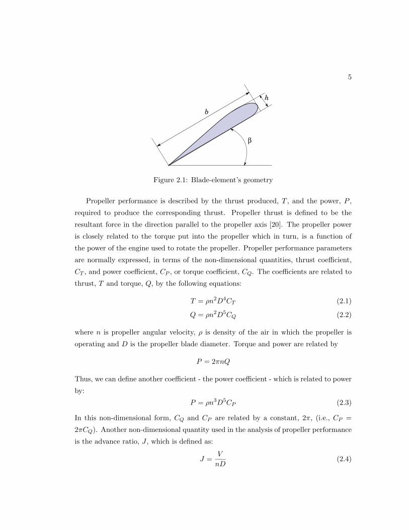
Figure 2.1: Blade-element’s geometry
Propeller performance is described by the thrust produced, T , and the power, P ,
required to produce the corresponding thrust. Propeller thrust is defined to be the
resultant force in the direction parallel to the propeller axis [20]. The propeller power
is closely related to the torque put into the propeller which in turn, is a function of
the power of the engine used to rotate the propeller. Propeller performance parameters
are normally expressed, in terms of the non-dimensional quantities, thrust coefficient,
CT , and power coefficient, CP , or torque coefficient, CQ. The coefficients are related to
thrust, T and torque, Q, by the following equations:
T = ρn2D4CT (2.1)
Q = ρn2D5CQ (2.2)
where n is propeller angular velocity, ρ is density of the air in which the propeller is
operating and D is the propeller blade diameter. Torque and power are related by
P = 2πnQ
Thus, we can define another coefficient - the power coefficient - which is related to power
by:
P = ρn3D5CP (2.3)
In this non-dimensional form, CQ and CP are related by a constant, 2π, (i.e., CP =
2πCQ). Another non-dimensional quantity used in the analysis of propeller performance
is the advance ratio, J , which is defined as:
J =V
nD(2.4)
6
where V is the forward speed of the aircraft, n is propeller angular velocity and D is
propeller diameter. The advance ratio is normally used as the independent parameter
from which the dependent parameters CT , CQ, and CP .
2.2 Momentum Theory
The momentum theory model attempts predict thrust by estimating the momentum
change of the airflow that occurs as it passes through the propeller. To this end, the
rotating propeller is idealized as an actuator disc; a device which produces thrust by
accelerating the air in front of the disk so that it has a larger momentum as it leaves
behind the disc. From Newton’s second law it follows that a force (thrust) will be
produced as a result of this momentum change. Momentum theory is one of the simplest
theories to analyze propeller performance. Rankine and R. E. Froude developed this
simple momentum theory [21] and its main parameter is the mass flow of air through the
disc. Froude developed his theory based on the existence of the actuator disc meanwhile
Rankine developed it by dividing this disc into many annular rings. Since this theory
has only one parameter - the flow of the air - it can only represent an ideal performance
of the propeller.
V
V
V V + w
p
actuator disc
V + w'
p
p
p' + dpp' p
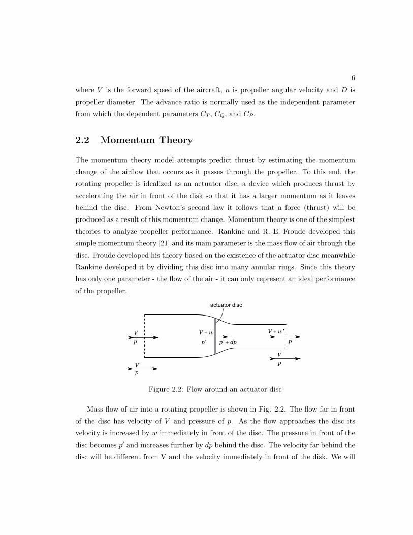
Figure 2.2: Flow around an actuator disc
Mass flow of air into a rotating propeller is shown in Fig. 2.2. The flow far in front
of the disc has velocity of V and pressure of p. As the flow approaches the disc its
velocity is increased by w immediately in front of the disc. The pressure in front of the
disc becomes p′ and increases further by dp behind the disc. The velocity far behind the
disc will be different from V and the velocity immediately in front of the disk. We will
7
model this velocity magnitude change in front and far behind the propeller disc as V +w
and V + w′, respectively. The quantities w and w′ are called the induced velocities in
front and far behind the propeller, respectively. If known, they characterize the thrust
production of a given propeller.
Applying Bernoulli’s principle, the propeller performance equations can be derived.
According to Bernoulli’s principle, there must be a discontinuity at the actuator disc.
The total pressure far in front of the disc and immediately in front of the disc are the
same. The total pressure far behind the disc and immediately behind the disc are the
same. Let us denoted C1 and C2 to be the total pressure in front of and behind the
disc, respectively. Then using Bernoulli’s principle, we can write:
C1 = p+1
2ρV 2 = p′ +
1
2ρ(V + w)2 (2.5)
C2 = p′ + dp+1
2ρ(V + w)2 = p+
1
2ρ(W + w′)2 (2.6)
Then, the total pressure difference at the actuator disc is
∆p = C2 − C1 = p+1
2ρ(V + w′)2 − p− 1
2ρV 2 = ρw′
(V +
w′
2
)(2.7)
Let A be the area of the actuator disc which is a function of propeller diameter or
A = πD2/4. For the moment, we will write this just as A. Then the thrust produced
by the propeller is
T = ∆pA = ρAw′(V +
w′
2
)(2.8)
To relate w′ to w, another equation for thrust can be derived from the rate of change
of axial momentum. That is,
T = m× ∆Velocity = ρA(V + w) × [V + w′ − V ] = ρA(V + w)w′ (2.9)
Using Eq.2.8 and Eq.2.9, the relation between w and w′ can be determined by:
T = ρAw′(V +
w′
2
)= ρA(V + w)w′
and, thus,
w′ = 2w (2.10)

8
The induced velocity, w, can be determined using this momentum theory. To do this,
we can rewrite Eq.2.9 by using Eq.2.10 as follows:
w2 + V w − T
2ρA= 0
Solving the quadratic equation above for w,
w = −1
2
[−V +
√V 2 +
2T
ρA
](2.11)
The second solution for the quadratic equation (i.e., w < 0) is ignored because it does
not make physical sense. Since V is the freestream or forward velocity, then w will be
maximum when the aircraft is not moving forward. Thus, we can solve for the induced
velocity and it will be directly proportional to the thrust produced. That is,
w =
√T
2ρA(2.12)
From basic thermodynamics we know that power added into the flow is the rate
of change of work done on the fluid. Considering the flow immediately in front of the
propeller, the power imparted to the flow (or induced in the flow) by the propeller is
called the induced power, Pi, and is given by
Pi = ∆pA(V + w)
Using Eq.2.7 and Eq.2.10 we can rewrite this as:
Pi = ρw′(V +
w′
2
)A(V + w) = ρAw′(V + w)2 (2.13)
The thrust produced by the propeller pushes the vehicle it is attached to forward at a
velocity V . Thus, the net power output of the propeller (denote Po) is equal to:
Po = TV = ρAw′(V + w)V
Note that Po is not necessarily equal to Pi. That is, some of the energy that is imparted
to the flowing air is lost and does not end up producing thrust. For example, some of it
goes to imparting rotational motion to the air which is not useful in producing thrust.
9
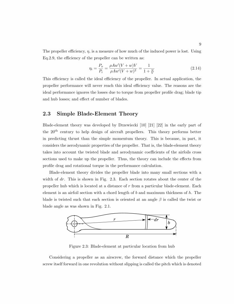
The propeller efficiency, η, is a measure of how much of the induced power is lost. Using
Eq.2.9, the efficiency of the propeller can be written as:
ηi =PoPi
=ρAw′(V + w)V
ρAw′(V + w)2=
1
1 + wV
(2.14)
This efficiency is called the ideal efficiency of the propeller. In actual application, the
propeller performance will never reach this ideal efficiency value. The reasons are the
ideal performance ignores the losses due to torque from propeller profile drag; blade tip
and hub losses; and effect of number of blades.
2.3 Simple Blade-Element Theory
Blade-element theory was developed by Drzewiecki [10] [21] [22] in the early part of
the 20th century to help design of aircraft propellers. This theory performs better
in predicting thrust than the simple momentum theory. This is because, in part, it
considers the aerodynamic properties of the propeller. That is, the blade-element theory
takes into account the twisted blade and aerodynamic coefficients of the airfoils cross
sections used to make up the propeller. Thus, the theory can include the effects from
profile drag and rotational torque in the performance calculation.
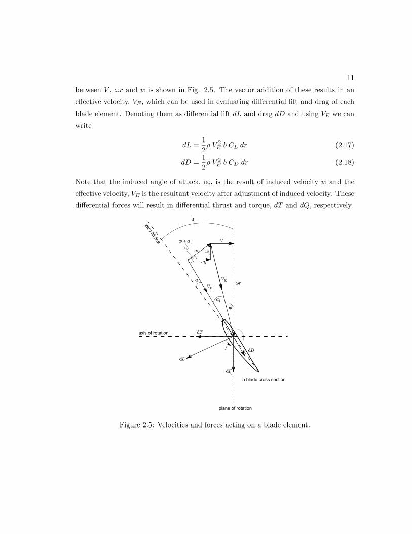
Blade-element theory divides the propeller blade into many small sections with a
width of dr. This is shown in Fig. 2.3. Each section rotates about the center of the
propeller hub which is located at a distance of r from a particular blade-element. Each
element is an airfoil section with a chord length of b and maximum thickness of h. The
blade is twisted such that each section is oriented at an angle β is called the twist or
blade angle as was shown in Fig. 2.1.
drr
R
b
Figure 2.3: Blade-element at particular location from hub
Considering a propeller as an airscrew, the forward distance which the propeller
screw itself forward in one revolution without slipping is called the pitch which is denoted

10
as p. As shown in Fig. 2.4, the screw motion of blade element is the helical path AA′
and its length p is given by [20]:
p = 2πr tanβ
It is customary to normalize pitch by propeller diameter. This quantity is called pitch-
diameter ratio and is given by:p
D= πx tanβ (2.15)
where x = 2r/D is the location of each blade-element as a fraction of propeller diameter.
For a constant pitch propeller, the value of p is constant along the blade. This implies
that the blade has a twist angle which varies along its length according to the following
expression:
β = tan−1(p/D
πx
)(2.16)
A
A'
r
A
A'
p
2πr
β
p^
Figure 2.4: Helical path of blade-element’s motion
A propeller blade performs two motion at the same time - a forward motion along
with the aircraft, V , and rotation about the center of the hub, ωr. Due to these two
motions, the blade section experiences a resultant velocity of magnitude VR, oriented
at an angle φ with respect to plane of rotation. Looking at each blade section as an
airfoil with air flow passing through it, the airfoil will produce a differential aerodynamic
force. However, if we are to consider the aerodynamics of each blade-element, we need
to consider the effect of the induced velocity as well. The induced velocity, w, is the
increase of the velocity of the air as it approaches the propeller. The vector addition
11
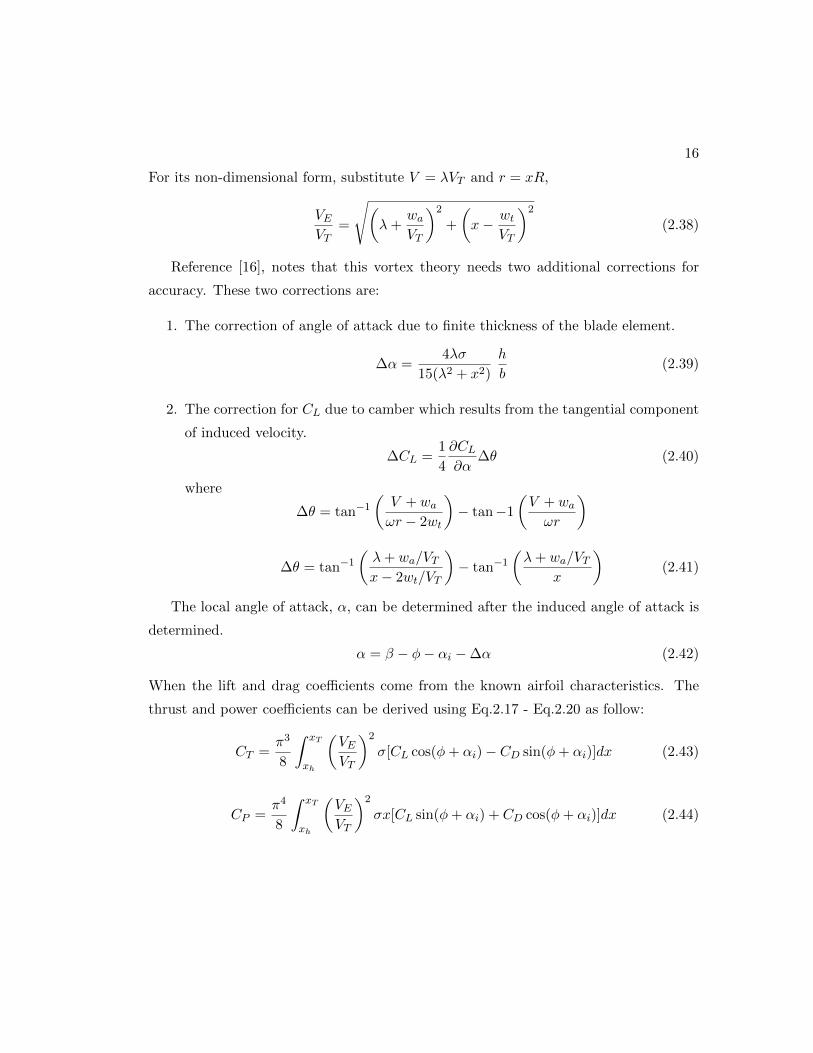
between V , ωr and w is shown in Fig. 2.5. The vector addition of these results in an
effective velocity, VE , which can be used in evaluating differential lift and drag of each
blade element. Denoting them as differential lift dL and drag dD and using VE we can
write
dL =1
2ρ V 2
E b CL dr (2.17)
dD =1
2ρ V 2
E b CD dr (2.18)
Note that the induced angle of attack, αi, is the result of induced velocity w and the
effective velocity, VE is the resultant velocity after adjustment of induced velocity. These
differential forces will result in differential thrust and torque, dT and dQ, respectively.
axis of rotation
zero lift line
a blade cross section
plane of rotation
w w
w
t
a
VR
VE
V
Γ
α
i
dD
dL
dT
dFQ
ωr
β
α
φ
iφ + α
Figure 2.5: Velocities and forces acting on a blade element.

12
Using Fig. 2.5, the differential thrust and torque can be expressed as
dT = dL cos(φ+ αi) − dD sin(φ+ αi) (2.19)
dQ = r[dL sin(φ+ αi) + dD cos(φ+ αi)] (2.20)
From Eq.2.19 and Eq.2.20, we note that if we know the lift and drag polars for the
airfoil cross section used to make the propeller as well as the induced velocity (for
induced angle of attack), then we can numerically integrate these equations to predict
thrust and torque. The challenge is to calculate w or αi. We can address this challenge
by combining blade element and momentum theories as we will do next.
2.4 Combined Momentum - Blade Element Theory
A modified theory which combines blade element theory with the momentum theory
is called the combined momentum - blade element theory. The momentum theory
contributes to the computation of the induced velocity which will give the information
needed to compute induced angle of attack. From the momentum theory, we will rewrite
Eq.2.8 as follow:
T = 2ρA(V + w)w (2.21)
A simplification to Eq.2.19 can be made by assuming that the induce angle of attack
and drag-to-lift ratio are small such that VE ≈ VR. Thus, Eq.2.19 can be used to
approximate the differential thrust for B blades. Substituting Eq.2.17 into Eq.2.19,
dT = B1
2ρ V 2
R b CL cosφ dr (2.22)
Noting that A = πr2, we can derive a differential thrust expression using Eq.2.21. This
gives:
dT = d(2ρ(πr2)(V + w)w) = 2ρ(2πr dr)(V + w)w (2.23)
The induced velocity can be approximated as w = VRαi cosφ. Using this in Eq.2.23
gives:
dT = 2ρ(2πr dr)(V + VR αi cosφ)VR αi cosφ (2.24)
Equating Eq.2.22 with Eq.2.24, the expression for induced angle of attack can be derived.
That is,
B1
2ρ V 2
R b CL cosφ dr = ρ(2πr dr)(V + VR αi cosφ)2VR αi cosφ

13
Rearranging the expression above and substituting CL = CLα(β − φ− αi),
B VR b CLα(β − φ− αi) = 8πrαi(V + VR αi cosφ) (2.25)
For simplicity of the mathematical expressions, we will non-dimensionalize Eq.2.25 by
introducing the symbol σ called the solidity ratio and λ called local advance ratio. These
quantities are expressed as follow:
σ =2B
π
b
D(2.26)
λ =V
12ωD
=V
VT(2.27)
Furthermore, since VR is the resultant velocity of ωr and V , we will define the tip speed
ratio as:VRVT
=√λ2 + x2
Given these definitions, the flow angle φ is equal to
φ = tan−1(λ
x
)= tan−1
(J
πx
)(2.28)
Using these non-dimensional parameters, Eq.2.25 can be simplified and expressed as a
quadratic equation for induced angle of attack. That is,
α2i +
[λ
x+σCLαVR8x2VT
]αi −
σCLαVR2x2VT
(β − φ) = 0
Solving this equation gives the following expression for αi as a function of x:
αi =1
2
−(λx
+σCLα8x2
√λ2 + x2
)+
√(λ
x+σCLα8x2
√λ2 + x2
)2
+σCLα2x2
√λ2 + x2(β − φ)
(2.29)
The negative solution for αi is not used because it represents the case where the induced
velocity is in the direction of flight: A physical impossibility in normal flight.
Using αi, propeller performance parameters, thrust and power, can be computed by
numerical integration of Eq.2.17 - Eq.2.20.
T =
∫1
2ρ V 2
E B b [CL cos(φ+ αi) − CD sin(φ+ αi)] dr
P = ω
∫1
2ρ V 2
E B b r[CL sin(φ+ αi) + CD cos(φ+ αi)] dr

14
For computational purposes, it is preferred to have these parameters in non-dimensional
form. Using the definition given at the beginning of this chapter, we can write:
CT =π
8
∫ xT
xh
(J2 + π2x2)σ[CL cos(φ+ αi) − CD sin(φ+ αi)]dx (2.30)
CP =π
8
∫ xT
xh
πx(J2 + π2x2)σ[CL sin(φ+ αi) + CD cos(φ+ αi)]dx (2.31)
Eq.2.30 and Eq.2.31 can be solved by numerical integration from the station near the
hub, xh, to the station near the tip, xT .
2.5 Incorporating Vortex Theory
The blade element theory has a limitation resulting from at least two assumption. First,
it assumes that blade elements at different station do not affect the flow of each other.
Secondly, it assumes that w is normal to the propeller disc. The net effect of this is that
the estimate of w is not correct. Vortex theory provides a means by which the estimate
of w can be improved. The idea is akin to what is done in thin-airfoil theory [23] [24].
The blade is replaced by a bound vortex distribution and, thus, the interaction of the
flow at different sections can be accounted for.
Theodorsen[11] presented the solution of the optimum distribution for heavily loaded
propeller using the circulation distribution developed by Goldstein who had presented
the distribution for lightly loaded propeller. Using Goldstein’s vortex theory, the in-
duced velocity can be related to the bound vortex circulation, Γ, by
wt =BΓ
4πrκ(2.32)
where κ is Goldstein’s κ factor. This factor is normally given in tabulated form as
function of radial position, local advance ratio and number of blades. For details on
this, see references [11] and [17].
An approximation for Goldstein’s κ factor is Prandtl’s solution of tip loss factor.
Prandtl’s tip loss factor, F , gives good results for propellers that have a large number
of blades and operating at small advance ratio.
F =2
πcos−1 exp
[−B(1 − x)
2 sinφT
](2.33)

15
where φT is the flow angle at the tip and it is given by:
φT = tan−1V
VT
This gives us a way to estimate the tangential component of w. However, from Fig.
2.5 we know that the induced velocity ,w, consists of axial and tangential components,
wa and wt, respectively. They are related by
tan(αi + φ) =V + waωr − wt
=wtwa
We can solve the expression above to obtain an expression for wa as function of wt:
wa =1
2
[−V +
√V 2 + 4wt(ωr − wt)
]For computational purposes, wa can be expressed in a non-dimensional form as:
waVT
=1
2
[−λ+
√λ2 + 4
wtVT
(x− wt
VT
) ](2.34)
Once we calculate wa/VT , we can estimate wt. To calculate wt we start with Eq.2.32
where Goldstein’s κ factor can be substituted by Prandtl’s tip loss factor. The bound
circulation can calculated using Kutta-Joukowski theorem.
Γ =1
2bCLVE (2.35)
Thus, substituting Eq.2.35 into Eq.2.32 we can solve for wt/VT as:
wtVT
=BCL4πxF
VEVT
b
D(2.36)
The induced angle of attack, αi can now be computed by the following expression,
αi = tan−1(V + wawr − wt
)− φ
In non-dimensional form, this expression is given as:
αi = tan−1
(λ+ wa
VT
x− wtVT
)− φ (2.37)
From Fig. 2.5, the remaining parameters can be derived. For example, using simple
geometry we note that:
V 2E = (V + wa)
2 + (ωr − wt)2
16
For its non-dimensional form, substitute V = λVT and r = xR,
VEVT
=
√(λ+
waVT
)2
+
(x− wt
VT
)2
(2.38)
Reference [16], notes that this vortex theory needs two additional corrections for
accuracy. These two corrections are:
1. The correction of angle of attack due to finite thickness of the blade element.
∆α =4λσ
15(λ2 + x2)
h
b(2.39)
2. The correction for CL due to camber which results from the tangential component
of induced velocity.
∆CL =1
4
∂CL∂α
∆θ (2.40)
where
∆θ = tan−1(V + waωr − 2wt
)− tan−1
(V + waωr
)
∆θ = tan−1(λ+ wa/VTx− 2wt/VT
)− tan−1
(λ+ wa/VT
x
)(2.41)
The local angle of attack, α, can be determined after the induced angle of attack is
determined.
α = β − φ− αi − ∆α (2.42)
When the lift and drag coefficients come from the known airfoil characteristics. The
thrust and power coefficients can be derived using Eq.2.17 - Eq.2.20 as follow:
CT =π3
8
∫ xT
xh
(VEVT
)2
σ[CL cos(φ+ αi) − CD sin(φ+ αi)]dx (2.43)
CP =π4
8
∫ xT
xh
(VEVT
)2
σx[CL sin(φ+ αi) + CD cos(φ+ αi)]dx (2.44)
17
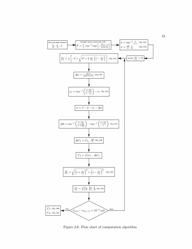
2.6 Computational Estimation of Propeller Performance
The propeller performance computation algorithm developed in this thesis is based on
the combination of blade element and vortex theory described in previous sections.
The inputs are the following propeller geometry parameters: Propeller diameter, blade
chord length, blade thickness, and blade pitch. The outputs are thrust coefficient, power
coefficient and efficiency.
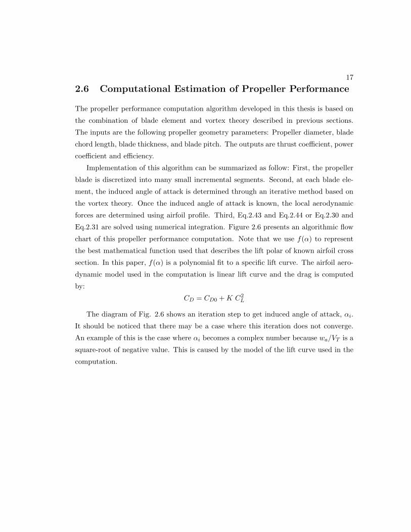
Implementation of this algorithm can be summarized as follow: First, the propeller
blade is discretized into many small incremental segments. Second, at each blade ele-
ment, the induced angle of attack is determined through an iterative method based on
the vortex theory. Once the induced angle of attack is known, the local aerodynamic
forces are determined using airfoil profile. Third, Eq.2.43 and Eq.2.44 or Eq.2.30 and
Eq.2.31 are solved using numerical integration. Figure 2.6 presents an algorithmic flow
chart of this propeller performance computation. Note that we use f(α) to represent
the best mathematical function used that describes the lift polar of known airfoil cross
section. In this paper, f(α) is a polynomial fit to a specific lift curve. The airfoil aero-
dynamic model used in the computation is linear lift curve and the drag is computed
by:
CD = CD0 +K C2L
The diagram of Fig. 2.6 shows an iteration step to get induced angle of attack, αi.
It should be noticed that there may be a case where this iteration does not converge.
An example of this is the case where αi becomes a complex number because wa/VT is a
square-root of negative value. This is caused by the model of the lift curve used in the
computation.
18
For4each4blade-element: PrandtlTs4tip4loss4factor4(Eq.42.33) (Eq.42.28)
(Eq.42.26)
(Eq.42.34) Assume
(Eq.42.39)
(Eq.42.37)
(Eq.42.38)
(Eq.42.41)
(Eq.42.40)
FalseTrue(Eq.42.30)
(Eq.42.31)
(Eq.42.36)
Figure 2.6: Flow chart of computation algorithm

Chapter 3
Experiment and Validation
In this chapter, the results of propeller performance computed using the method de-
scribed in previous chapter are validated using experiment data. The experiments were
performed using the wind tunnel facility as the University of Minnesota. This chap-
ter describes the experiment procedures, implementation of the algorithm developed in
previous chapter and discussion of both experimental and computational results.
3.1 Propeller Wind Tunnel Experiment
One of the methods to estimate propeller performance is to test the propeller in a wind
tunnel. A large number of full-scale propeller tests had been done by the National
Advisory Committee for Aeronautics (NACA) in 1930s and 1940s. This thesis explores
a full-scale propeller test for UAVs. The size of the propellers are much smaller than
the ones tested by NACA. Thus, part of the motivation for the work that follows is
to examine how different in size of the propeller affects the applicability of the NACA
historic test results on small propellers. In this section, we present procedures of thin
electric propeller test.
3.1.1 Apparatus and Methods
The experiments were conducted using a closed-return wind tunnel at the University
of Minnesota [25]. The wind tunnel is driven by 100 HP frequency controlled variable
speed electric motor with P-38 Feathering Propeller. This wind tunnel has a 40 × 60
19
20
inches test section. The wind tunnel is equipped with a sensor which measures three
axes of forces and three axes of torques.
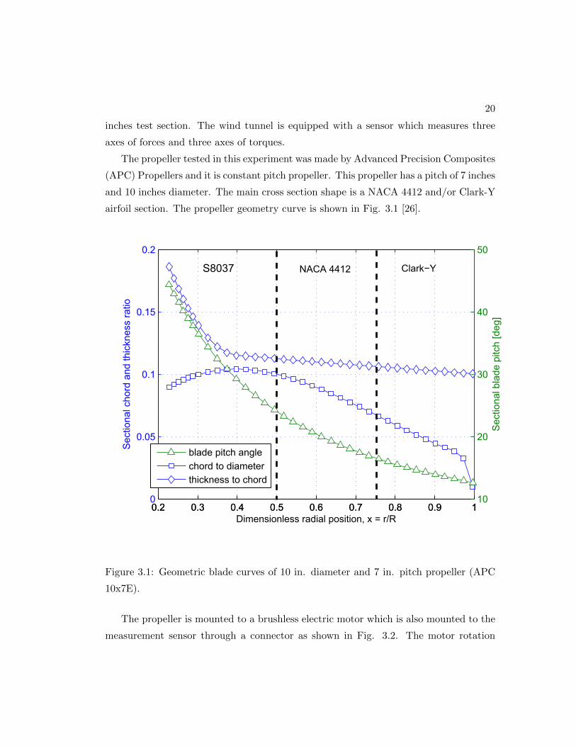
The propeller tested in this experiment was made by Advanced Precision Composites
(APC) Propellers and it is constant pitch propeller. This propeller has a pitch of 7 inches
and 10 inches diameter. The main cross section shape is a NACA 4412 and/or Clark-Y
airfoil section. The propeller geometry curve is shown in Fig. 3.1 [26].
0.2 0.3 0.4 0.5 0.6 0.7 0.8 0.9 10
0.05
0.1
0.15
0.2
DimensionlesscradialcpositionYcxc=cr/R
Sec
tiona
lccho
rdca
ndcth
ickn
essc
ratio
0.2 0.3 0.4 0.5 0.6 0.7 0.8 0.9 110
20
30
40
50
Sec
tiona
lcbla
decp
itchc
[deg
]
bladecpitchcangle
chordctocdiameter
thicknessctocchord
MHc102 NACAc4412 Clark−YS8037
Figure 3.1: Geometric blade curves of 10 in. diameter and 7 in. pitch propeller (APC
10x7E).
The propeller is mounted to a brushless electric motor which is also mounted to the
measurement sensor through a connector as shown in Fig. 3.2. The motor rotation
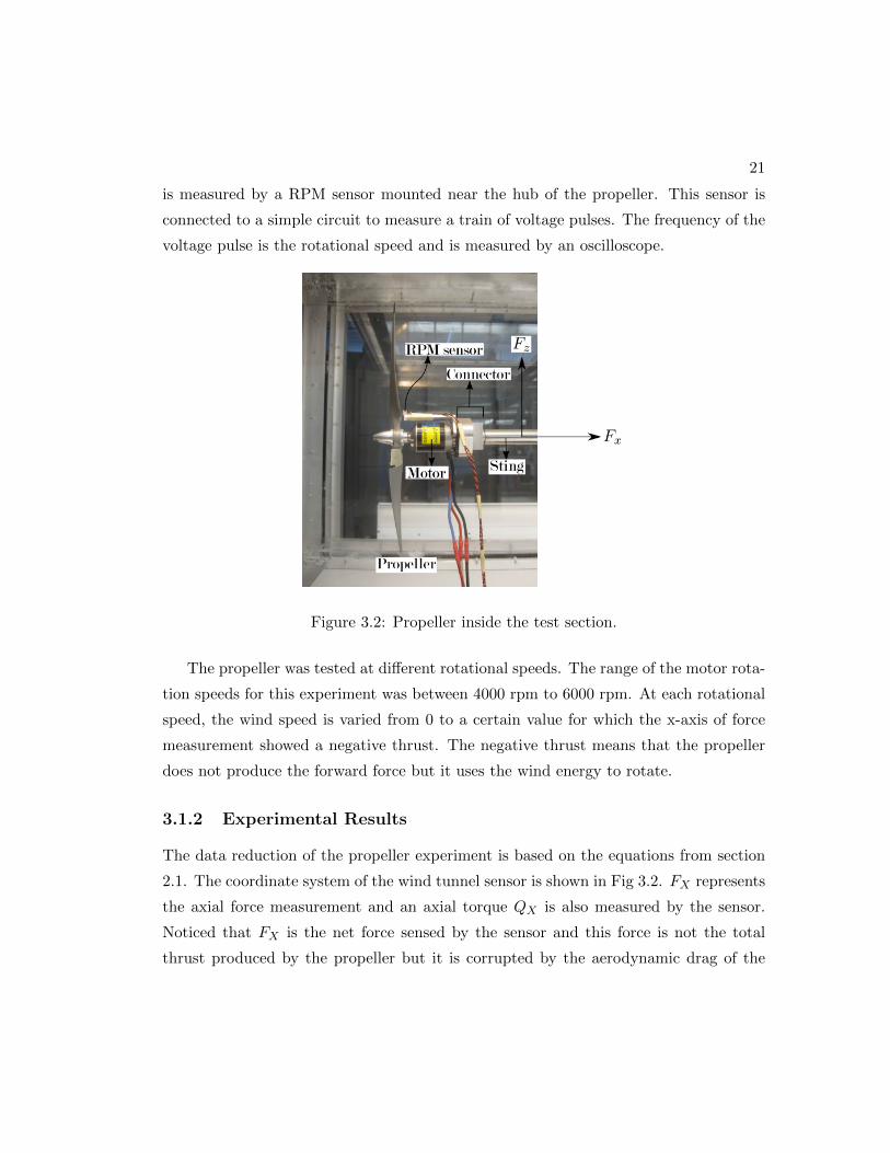
21
is measured by a RPM sensor mounted near the hub of the propeller. This sensor is
connected to a simple circuit to measure a train of voltage pulses. The frequency of the
voltage pulse is the rotational speed and is measured by an oscilloscope.
Figure 3.2: Propeller inside the test section.
The propeller was tested at different rotational speeds. The range of the motor rota-
tion speeds for this experiment was between 4000 rpm to 6000 rpm. At each rotational
speed, the wind speed is varied from 0 to a certain value for which the x-axis of force
measurement showed a negative thrust. The negative thrust means that the propeller
does not produce the forward force but it uses the wind energy to rotate.
3.1.2 Experimental Results
The data reduction of the propeller experiment is based on the equations from section
2.1. The coordinate system of the wind tunnel sensor is shown in Fig 3.2. FX represents
the axial force measurement and an axial torque QX is also measured by the sensor.
Noticed that FX is the net force sensed by the sensor and this force is not the total
thrust produced by the propeller but it is corrupted by the aerodynamic drag of the

22
rotating system or fixture drag, Fd. Thus, the thrust produced by the propeller is:
T = −FX + Fd
The fixture drag correction is based on the work done by Selig and Ananda [27].
Fd =1
2ρ (J n D)2 Sf Cdf
where Sf is the motor fixture frontal area and Cdf is assumed to be 1.
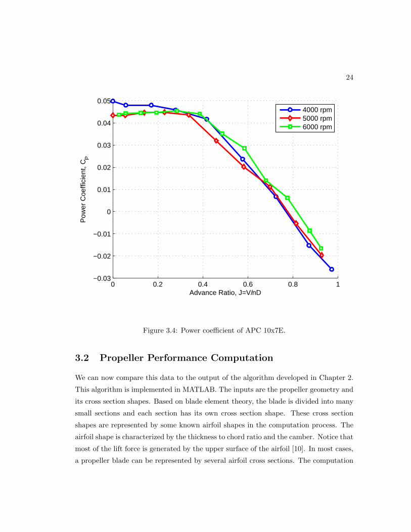
The experimental result of the propeller is shown in Fig. 3.3 and 3.4. These re-
sults show that the rotational speed affects the propeller performance due to Reynolds
numbers. At lower rotational speed, the blade operates at lower Reynolds number and
the Reynolds number increases as the rotational speed increases. Based on the airfoil
aerodynamics, the propeller becomes more efficient as the Reynolds number increases.

23
0 0.2 0.4 0.6 0.8 1−0.06
−0.04
−0.02
0
0.02
0.04
0.06
0.08
0.1
0.12
Advance Ratio, J=V/nD
Thr
ust C
oeffi
cien
t, C
T
4000 rpm5000 rpm6000 rpm
Figure 3.3: Thrust coefficient of APC 10x7E.
24
0 0.2 0.4 0.6 0.8 1−0.03
−0.02
−0.01
0
0.01
0.02
0.03
0.04
0.05
Advance Ratio, J=V/nD
Pow
er C
oeffi
cien
t, C
P
4000 rpm5000 rpm6000 rpm
Figure 3.4: Power coefficient of APC 10x7E.
3.2 Propeller Performance Computation
We can now compare this data to the output of the algorithm developed in Chapter 2.
This algorithm is implemented in MATLAB. The inputs are the propeller geometry and
its cross section shapes. Based on blade element theory, the blade is divided into many
small sections and each section has its own cross section shape. These cross section
shapes are represented by some known airfoil shapes in the computation process. The
airfoil shape is characterized by the thickness to chord ratio and the camber. Notice that
most of the lift force is generated by the upper surface of the airfoil [10]. In most cases,
a propeller blade can be represented by several airfoil cross sections. The computation
25
process is based on the description at the last section of Chapter 2.
3.2.1 APC 10x7E Propeller
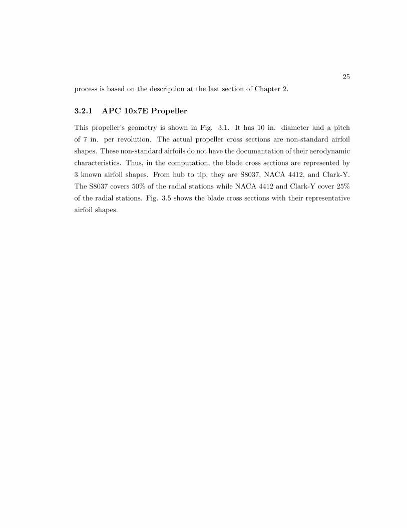
This propeller’s geometry is shown in Fig. 3.1. It has 10 in. diameter and a pitch
of 7 in. per revolution. The actual propeller cross sections are non-standard airfoil
shapes. These non-standard airfoils do not have the documantation of their aerodynamic
characteristics. Thus, in the computation, the blade cross sections are represented by
3 known airfoil shapes. From hub to tip, they are S8037, NACA 4412, and Clark-Y.
The S8037 covers 50% of the radial stations while NACA 4412 and Clark-Y cover 25%
of the radial stations. Fig. 3.5 shows the blade cross sections with their representative
airfoil shapes.

26
0 0.5 1
−0.2
0
0.2
0.4
S8037
0 0.5 1
−0.2
0
0.2
0.4NACA 4412
0 0.5 1
−0.2
0
0.2
0.4Clark−Y
Approximate airfoil sectionActual propeller cross section
Figure 3.5: Blade cross sections of APC 10x7E.
The performance of APC 10×7E can be computed by importing its geometry (shown
in Fig. 3.1) and selecting proper airfoil aerodynamics. The aerodynamics of the blade
cross sections are represented by the known airfoils as shown in Fig. 3.5. However, there
are some errors in the aerodynamic description. For example, the pitch angle assumed
in the model may be different from the actual pitch angle. Another error considered in
this regard is the slope of the lift curve for each blade element.

27
0.2 0.3 0.4 0.5 0.6 0.7 0.8 0.9 1−0.5
0
0.5
1
1.5
2
2.5x 10
−3
radial distance, x
dCT J
Figure 3.6: Sectional thrust coefficient of APC 10x7E.

28
0.2 0.3 0.4 0.5 0.6 0.7 0.8 0.9 1−10
−5
0
5
10
15
20
25
radial distance, x
loca
l ang
le o
f atta
ck, α
[deg
]
J
Figure 3.7: Sectional angle of attack of APC 10x7E.
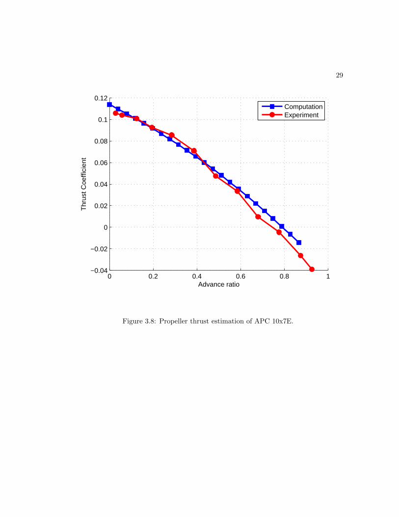
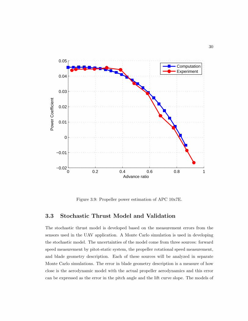
As a baseline a simulation using a nominal model is performed and compared to
experimental data. The computational result agrees with the experimental result as
shown in Fig. 3.8 and Fig. 3.9. The sectional thrust coefficient from Fig. 3.6 shows
that only a portion of the blade does most of the works. The sections near the root do
not contribute a lot of thrust. This shows that the approximation of the aerodynamics
of the sections near the root will not affect the result significantly. The local angle of
attack decreases as the advance ratio increases as shown in Fig. 3.7. The blade operates
at high angle of attack when the advance ratio is low and it operates at negative angle
of attack when the advance ratio is high. The static thrust coefficient is 0.1138 and the
static power coefficient is 0.0457. Both curves cross the zero line at advance ratio about
0.8.
29
0 0.2 0.4 0.6 0.8 1−0.04
−0.02
0
0.02
0.04
0.06
0.08
0.1
0.12
Advance ratio
Thr
ust C
oeffi
cien
t
ComputationExperiment
Figure 3.8: Propeller thrust estimation of APC 10x7E.
30
0 0.2 0.4 0.6 0.8 1−0.02
−0.01
0
0.01
0.02
0.03
0.04
0.05
Advance ratio
Pow
er C
oeffi
cien
t
ComputationExperiment
Figure 3.9: Propeller power estimation of APC 10x7E.
3.3 Stochastic Thrust Model and Validation
The stochastic thrust model is developed based on the measurement errors from the
sensors used in the UAV application. A Monte Carlo simulation is used in developing
the stochastic model. The uncertainties of the model come from three sources: forward
speed measurement by pitot-static system, the propeller rotational speed measurement,
and blade geometry description. Each of these sources will be analyzed in separate
Monte Carlo simulations. The error in blade geometry description is a measure of how
close is the aerodynamic model with the actual propeller aerodynamics and this error
can be expressed as the error in the pitch angle and the lift curve slope. The models of
31
the uncertainties are drawn from a zero-mean Gaussian noise with certain variance.
Two Monte Carlo simulations are conducted for sensor measurement error. The
first case is a simulation where the error is for the forward speed measurement and the
errors are drawn from a normal distribution with 0.5 m/s, 1 m/s and 2 m/s standard
deviations, respectively. The second case is for the rotational speed measurement error
and the values of the error are also drawn from a normal distribution with 50 rpm and
100 rpm standard deviations. The third case of the simulation is a simulation where the
error is from the blade geometry which includes the error in pitch and lift curve slope.
The pitch uncertainties are 1◦ and 2◦, respectively. The uncertainty in airfoil lift curve
slope is represented by the percentage of the nominal value which is also drawn from a
normal distribution with standard deviations of 0.05 and 0.15.
32
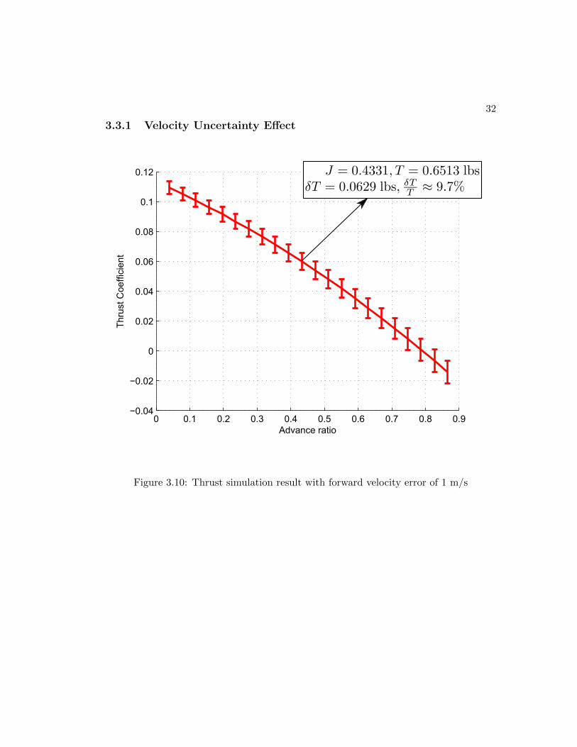
3.3.1 Velocity Uncertainty Effect
0 0.1 0.2 0.3 0.4 0.5 0.6 0.7 0.8 0.9−0.04
−0.02
0
0.02
0.04
0.06
0.08
0.1
0.12
Advance ratio
Thr
ust C
oeffi
cien
t
Figure 3.10: Thrust simulation result with forward velocity error of 1 m/s

33
0 0.1 0.2 0.3 0.4 0.5 0.6 0.7 0.8 0.92
4
6
8
10
12
14
16x 10
−3
Advance ratio
Sta
ndar
d D
evia
tion
of th
rust
coe
ffici
ent
σV = 0.5 m/s
σV = 1 m/s
σV = 2 m/s
Figure 3.11: Error variation in thrust with advance ratio
34
0 0.1 0.2 0.3 0.4 0.5 0.6 0.7 0.8 0.9−0.02
−0.01
0
0.01
0.02
0.03
0.04
0.05
Advance ratio
Pow
er C
oeffi
cien
t
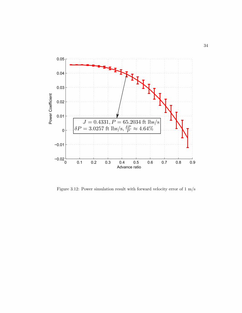
Figure 3.12: Power simulation result with forward velocity error of 1 m/s

35
0 0.1 0.2 0.3 0.4 0.5 0.6 0.7 0.8 0.90
0.002
0.004
0.006
0.008
0.01
0.012
0.014
Advance ratio
Sta
ndar
d D
evia
tion
of p
ower
coe
ffici
ent
σV = 0.5 m/s
σV = 1 m/s
σV = 2 m/s
Figure 3.13: Error variation in power with advance ratio
The simulation results of forward velocity error are shown in Fig. 3.10 through Fig. 3.13.
The error drawn from N(0, (1 m/s)2) has a significant effect to the thrust predicted as
shown by the error bar of Fig. 3.10. Figure 3.11 shows that the thrust coefficient error
increases as the advance ratio increases. The thrust coefficient error is proportional to
the forward velocity error. It is also linear in advance ratio for small σV . The power
coefficient error increases as the advance ratio increase and its increment is non-linear
as shown by Fig. 3.12 and Fig. 3.13. The power coefficient error is proportional to the
forward velocity error.

36
3.3.2 Rotational Speed Uncertainty Effect
0 0.1 0.2 0.3 0.4 0.5 0.6 0.7 0.8 0.9−0.02
0
0.02
0.04
0.06
0.08
0.1
0.12
Advance ratio
Thr
ust C
oeffi
cien
t
Figure 3.14: Thrust simulation result with rotational speed error of 50 rpm
37
0 0.1 0.2 0.3 0.4 0.5 0.6 0.7 0.8 0.90
0.5
1
1.5
2
2.5
3x 10
−3
Advance ratio
Sta
ndar
d D
evia
tion
of th
rust
coe
ffici
ent
σ
n = 50 rpm
σn = 100 rpm
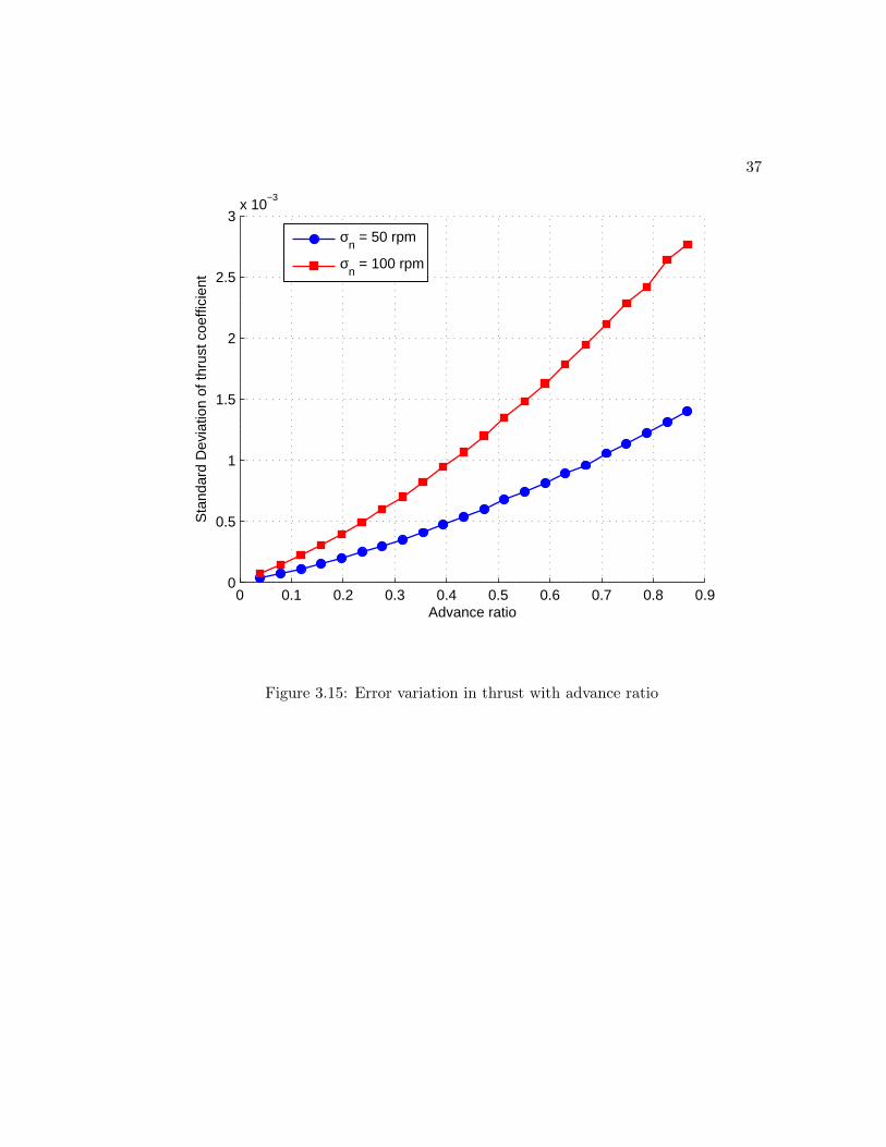
Figure 3.15: Error variation in thrust with advance ratio
38
0 0.1 0.2 0.3 0.4 0.5 0.6 0.7 0.8 0.9−0.01
0
0.01
0.02
0.03
0.04
0.05
Advance ratio
Pow
er C
oeffi
cien
t
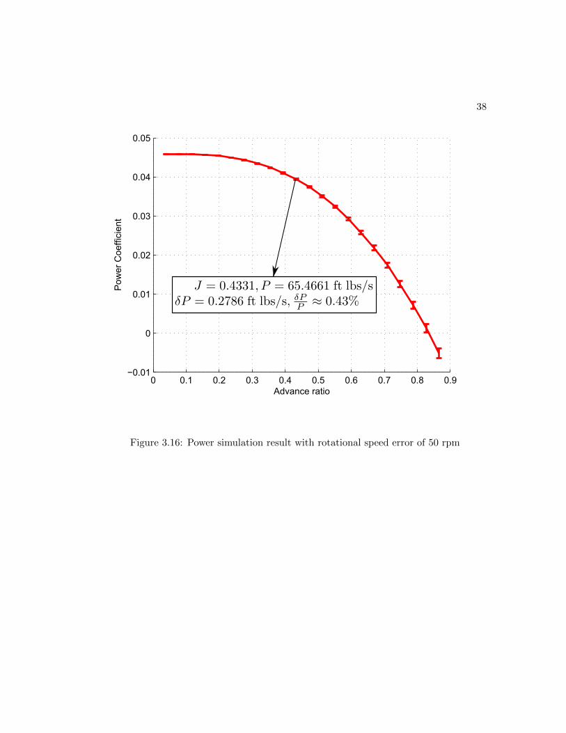
Figure 3.16: Power simulation result with rotational speed error of 50 rpm

39
0 0.1 0.2 0.3 0.4 0.5 0.6 0.7 0.8 0.90
0.5
1
1.5
2
2.5x 10
−3
Advance ratio
Sta
ndar
d D
evia
tion
of p
ower
coe
ffici
ent
σ
n = 50 rpm
σn = 100 rpm
Figure 3.17: Error variation in power with advance ratio
Figures 3.14 to 3.17 show the simulation results for rotational speed error. The rota-
tional speed error in this case drawn from N(0, (50 rpm)2) does not affect the results
significantly as shown by Fig. 3.14 and Fig. 3.16. For this case, the error is small
and negligible. Figures 3.15 and 3.17 show that the thrust and power coefficient errors
increase as the advance ratio increases, respectively. The thrust and power coefficient
error are proportional to the rotational speed error and non-linear with advance ratio.
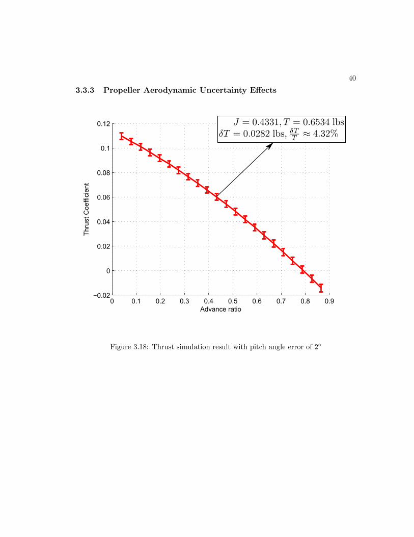
40
3.3.3 Propeller Aerodynamic Uncertainty Effects
0 0.1 0.2 0.3 0.4 0.5 0.6 0.7 0.8 0.9−0.02
0
0.02
0.04
0.06
0.08
0.1
0.12
Advance ratio
Thr
ust C
oeffi
cien
t
Figure 3.18: Thrust simulation result with pitch angle error of 2◦
41
0 0.1 0.2 0.3 0.4 0.5 0.6 0.7 0.8 0.91.2
1.4
1.6
1.8
2
2.2
2.4
2.6
2.8
3
3.2x 10
−3
Advance ratio
Sta
ndar
d D
evia
tion
of th
rust
coe
ffici
ent
σβ = 1o
σβ = 2o
Figure 3.19: Error variation in thrust with advance ratio

42
0 0.1 0.2 0.3 0.4 0.5 0.6 0.7 0.8 0.9−0.01
0
0.01
0.02
0.03
0.04
0.05
Advance ratio
Pow
er C
oeffi
cien
t
Figure 3.20: Power simulation result with pitch angle error of 2◦
43
0 0.1 0.2 0.3 0.4 0.5 0.6 0.7 0.8 0.90.6
0.8
1
1.2
1.4
1.6
1.8
2
2.2
2.4
2.6x 10
−3
Advance ratio
Sta
ndar
d D
evia
tion
of p
ower
coe
ffici
ent
σβ = 1o
σβ = 2o
Figure 3.21: Error variation in power with advance ratio
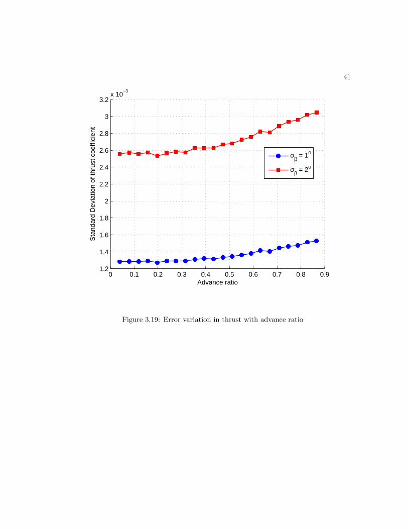
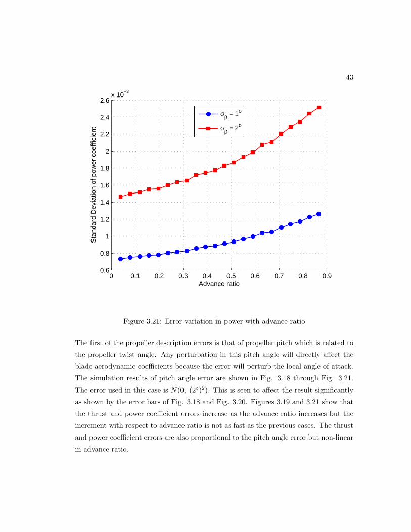
The first of the propeller description errors is that of propeller pitch which is related to
the propeller twist angle. Any perturbation in this pitch angle will directly affect the
blade aerodynamic coefficients because the error will perturb the local angle of attack.
The simulation results of pitch angle error are shown in Fig. 3.18 through Fig. 3.21.
The error used in this case is N(0, (2◦)2). This is seen to affect the result significantly
as shown by the error bars of Fig. 3.18 and Fig. 3.20. Figures 3.19 and 3.21 show that
the thrust and power coefficient errors increase as the advance ratio increases but the
increment with respect to advance ratio is not as fast as the previous cases. The thrust
and power coefficient errors are also proportional to the pitch angle error but non-linear
in advance ratio.
44
0 0.1 0.2 0.3 0.4 0.5 0.6 0.7 0.8 0.9−0.02
0
0.02
0.04
0.06
0.08
0.1
0.12
Advance ratio
Thr
ust C
oeffi
cien
t
Figure 3.22: Thrust simulation result with lift curve slope error of 15%
45
0 0.1 0.2 0.3 0.4 0.5 0.6 0.7 0.8 0.90
0.2
0.4
0.6
0.8
1
1.2
1.4
1.6
1.8x 10
−3
Advance ratio
Sta
ndar
d D
evia
tion
of th
rust
coe
ffici
ent
σC
Lα
= 0.05CLα
σC
Lα
= 0.15CLα
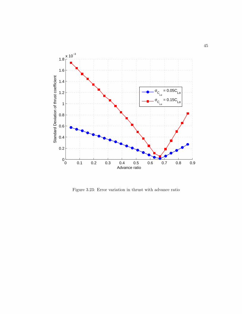
Figure 3.23: Error variation in thrust with advance ratio
46
0 0.1 0.2 0.3 0.4 0.5 0.6 0.7 0.8 0.9−0.01
0
0.01
0.02
0.03
0.04
0.05
Advance ratio
Pow
er C
oeffi
cien
t
Figure 3.24: Power simulation result with lift curve slope error of 15%
47
0 0.1 0.2 0.3 0.4 0.5 0.6 0.7 0.8 0.90
0.1
0.2
0.3
0.4
0.5
0.6
0.7
0.8
0.9
1x 10
−3
Advance ratio
Sta
ndar
d D
evia
tion
of p
ower
coe
ffici
ent
σC
Lα
= 0.05CLα
σC
Lα
= 0.15CLα
Figure 3.25: Error variation in power with advance ratio
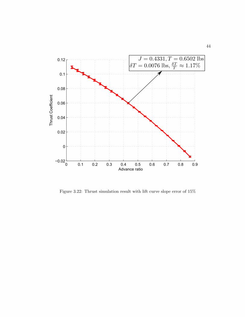
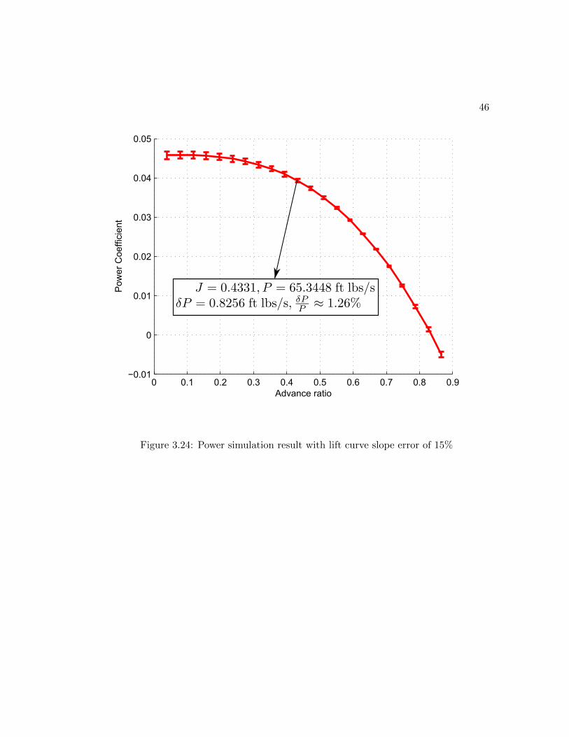
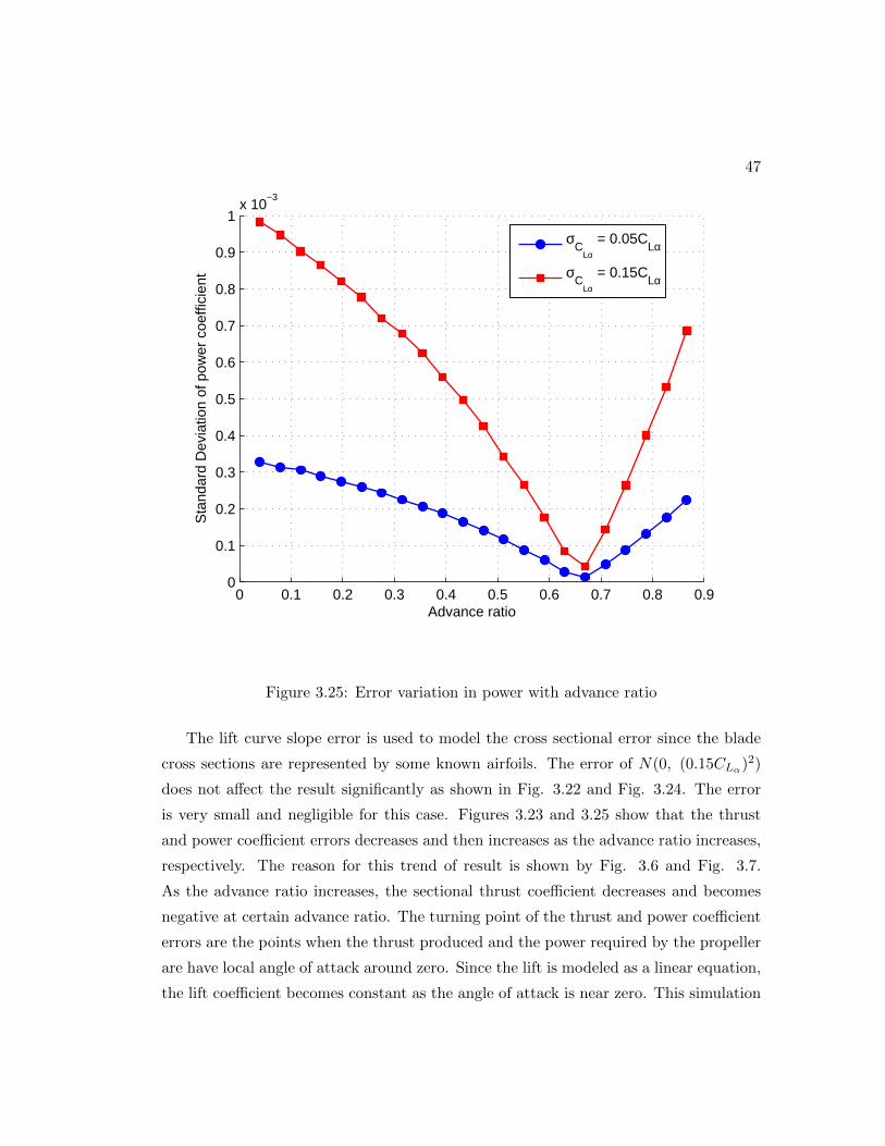
The lift curve slope error is used to model the cross sectional error since the blade
cross sections are represented by some known airfoils. The error of N(0, (0.15CLα)2)
does not affect the result significantly as shown in Fig. 3.22 and Fig. 3.24. The error
is very small and negligible for this case. Figures 3.23 and 3.25 show that the thrust
and power coefficient errors decreases and then increases as the advance ratio increases,
respectively. The reason for this trend of result is shown by Fig. 3.6 and Fig. 3.7.
As the advance ratio increases, the sectional thrust coefficient decreases and becomes
negative at certain advance ratio. The turning point of the thrust and power coefficient
errors are the points when the thrust produced and the power required by the propeller
are have local angle of attack around zero. Since the lift is modeled as a linear equation,
the lift coefficient becomes constant as the angle of attack is near zero. This simulation

48
result shows that this type of error can be neglected if the actual blade cross section is
known and well modeled.
Chapter 4
Stochastic Model of Aircraft
Dynamics
Aircraft dynamics is a term used to describe the aircraft’s behaviour in flight and its
mathematical representation are the equations of motion. These equations of motion
consist of aerodynamic coefficients, stability and control derivatives. As stated in the
beginning of this thesis, the aircraft’s equations of motion can be empirically determined
by using a computational software, such as DATCOM[7]. To get more accurate aircraft
dynamics, wind tunnel experiments are required for determining the parameters in the
aircraft’s equations of motion. This chapter explores the wind tunnel experiment on
a small UAV (Mini-Ultrastick) and developing its stochastic aircraft dynamic model
based on measurement errors.
4.1 Wind Tunnel Experiment
In general, the objective of this wind tunnel experiment is to determine the aircraft’s
aerodynamics. The parameters in aircraft’s equations of motion can be computed using
the experiment results. In this case, this experiment is performed using the closed-
return wind tunnel facility at the University of Minnesota. This wind tunnel has a
40 × 60 inches test section. It is powered by 100 HP frequency controlled variable
speed electric motor with P-38 Feathering Propeller. It is equipped with a six degree
of freedom force balance (sting) to measure three axes of forces and moments. A pitot
49

50
probe for measuring airspeed is mounted at the beginning of the test section. The air
pressure information is coming from a pressure server. The angle of attack is measured
by an inclinometer. All of these outputs are processed by a data acquisition computer.
Figure 4.1: Mini-Ultrastick inside wind tunnel test section.
A small UAV (Mini-Ultrastick) is mounted on the sting inside the test section as
shown in Fig. 4.1. This UAV has four control surfaces controlled by servos (ailerons,
elevator, rudder, and flaps). In this experiment, there are only two control surfaces being
used; elevator and rudder. Each control surface will only be deflected at its maximum,
neutral, and minimum deflections. The deflection limits of elevator and rudder are
±18◦ and ±30◦, respectively. This experiment is performed such that there is only one
control surface being deflected at each data acquisition. The angle of attack is varied
form −10◦ to 22◦. The tunnel speed is set at a constant speed of 8 m/s. The center
of force and moment measurements are located and the sting’s moment center (MC) as
shown in Fig. 4.2. Since the measurement center of interest is the aircraft’s center of
gravity (CG), all of the measurements will be transferred from MC to CG.
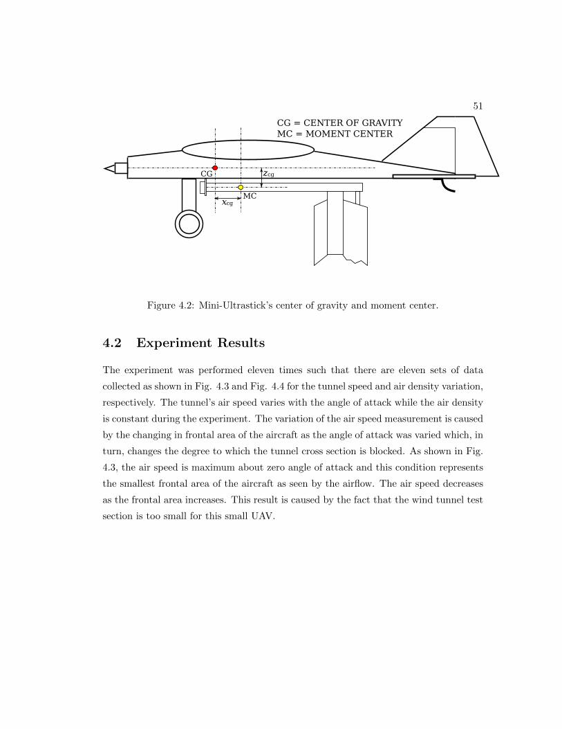
51
CG
MC
CG = CENTER OF GRAVITY
MC = MOMENT CENTER
xcg
zcg
Figure 4.2: Mini-Ultrastick’s center of gravity and moment center.
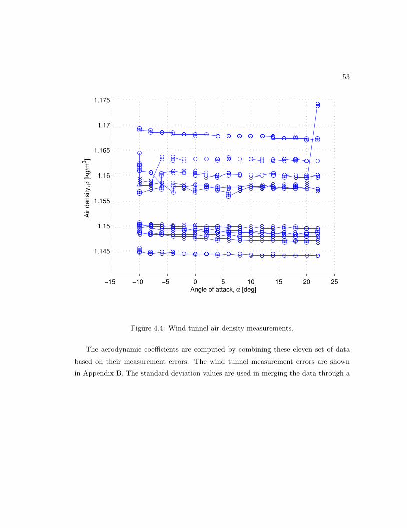
4.2 Experiment Results
The experiment was performed eleven times such that there are eleven sets of data
collected as shown in Fig. 4.3 and Fig. 4.4 for the tunnel speed and air density variation,
respectively. The tunnel’s air speed varies with the angle of attack while the air density
is constant during the experiment. The variation of the air speed measurement is caused
by the changing in frontal area of the aircraft as the angle of attack was varied which, in
turn, changes the degree to which the tunnel cross section is blocked. As shown in Fig.
4.3, the air speed is maximum about zero angle of attack and this condition represents
the smallest frontal area of the aircraft as seen by the airflow. The air speed decreases
as the frontal area increases. This result is caused by the fact that the wind tunnel test
section is too small for this small UAV.

52
−15 −10 −5 0 5 10 15 20 257.2
7.4
7.6
7.8
8
8.2
8.4
8.6
Angle of attack, α [deg]
Airspeed, V
[m
/s]
Figure 4.3: Wind tunnel speed measurements.
53
−15 −10 −5 0 5 10 15 20 25
1.145
1.15
1.155
1.16
1.165
1.17
1.175
Angle of attack, α [deg]
Air d
ensity, ρ
[kg/m
3]
Figure 4.4: Wind tunnel air density measurements.
The aerodynamic coefficients are computed by combining these eleven set of data
based on their measurement errors. The wind tunnel measurement errors are shown
in Appendix B. The standard deviation values are used in merging the data through a

54
linearized filter. The aerodynamic equations used in data reduction are shown below:
D = −FX cosα− FZ sinα =1
2ρ V 2 Sw CD (4.1)
Y = FY =1
2ρ V 2 Sw CY (4.2)
L = FX sinα− FZ cosα =1
2ρ V 2 Sw CL (4.3)
Lcg = MX − zcg FY =1
2ρ V 2 Sw bw Cl (4.4)
Mcg = MY + zcg FX =1
2ρ V 2 Sw cw Cm (4.5)
Ncg = MZ + xcg FY =1
2ρ V 2 Sw bw Cn (4.6)
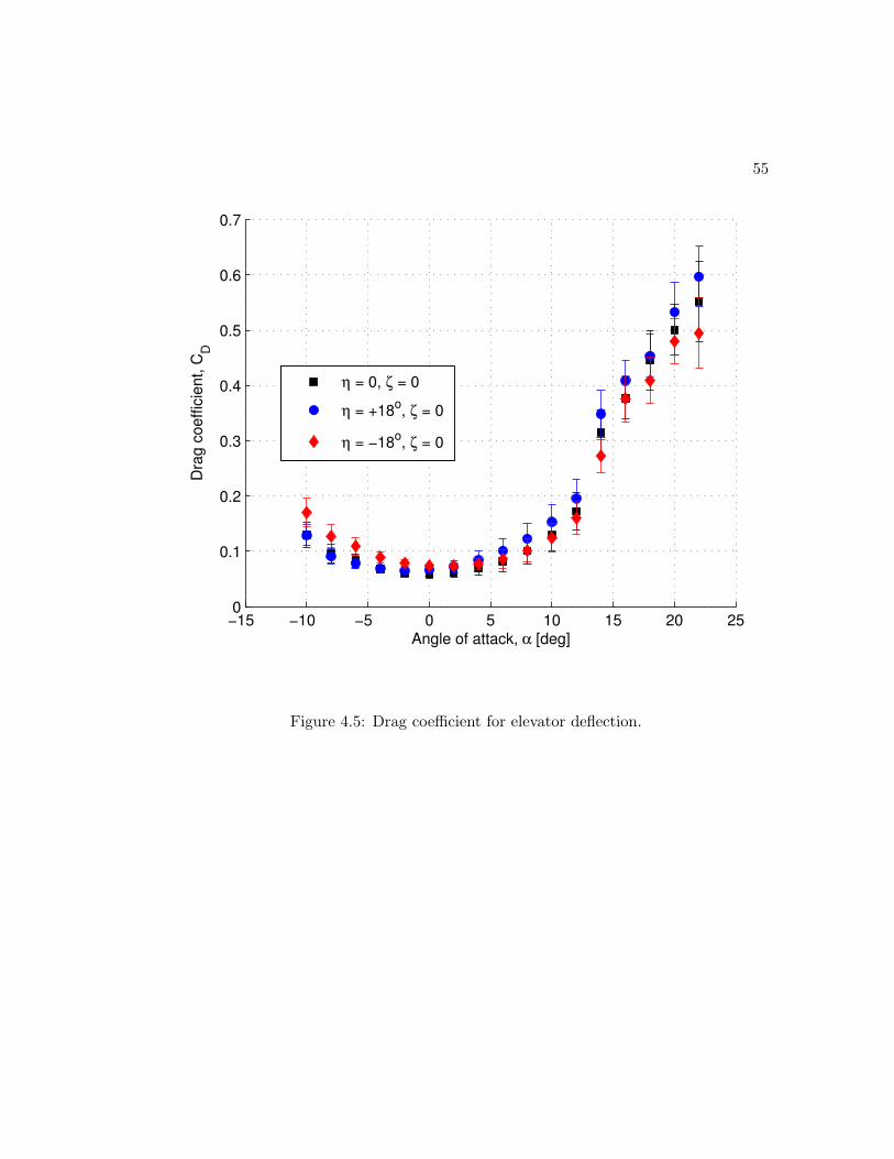
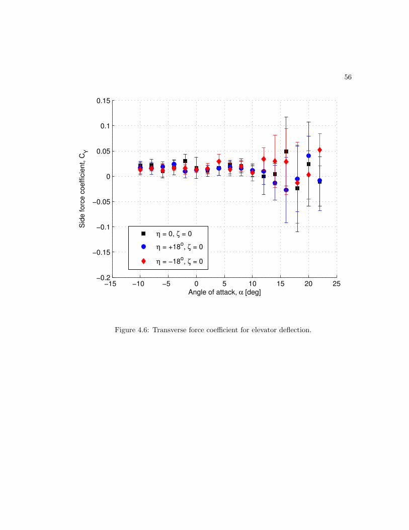
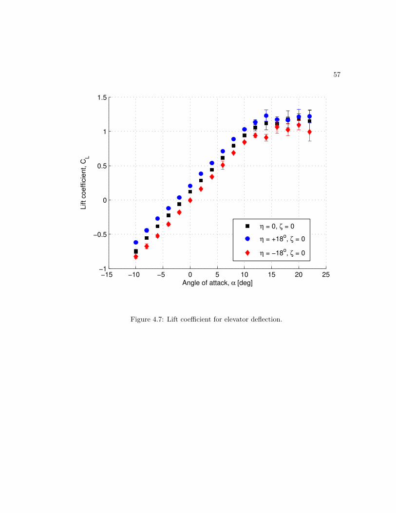
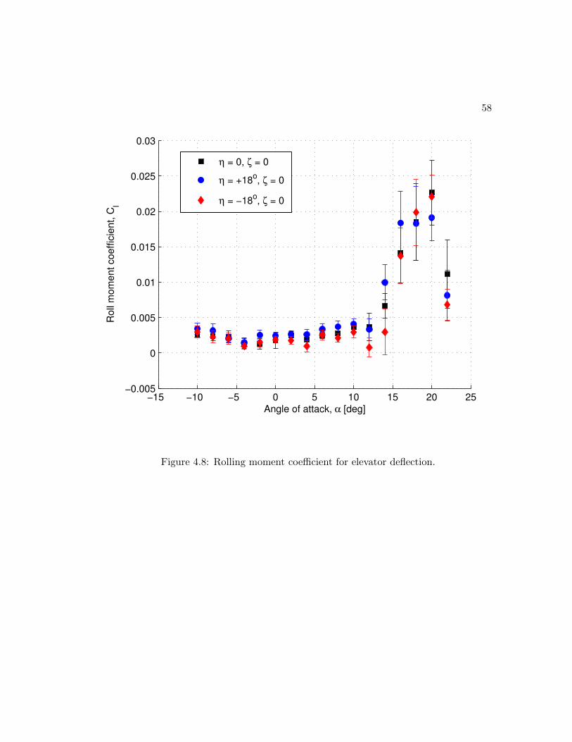
The experiment results for elevator deflection are plotted from Fig. 4.5 to Fig. 4.10.
This elevator deflection affects the lift and the pitching moment of the aircraft. A posi-
tive elevator deflection causes an increase in lift and a decrease in pitching moment while
a negative one will do the opposite as shown in Fig. 4.7 and Fig.4.9 for lift coefficient
and pitching moment coefficient, respectively. The plots of drag coefficient and pitching
moment coefficient clearly show when the aircraft enters into stall condition. The drag
coefficient shows that there is a sudden increase in drag between angle of attack of 12◦
and 14◦ as shown in Fig. 4.5. This trend also can be seen in Fig. 4.9. The stall region
is also marked by the high standard deviation values as shown by the y-axis error bar.
55
−15 −10 −5 0 5 10 15 20 250
0.1
0.2
0.3
0.4
0.5
0.6
0.7
Angle of attack, α [deg]
Dra
g c
oeffic
ient, C
D
η = 0, ζ = 0
η = +18o, ζ = 0
η = −18o, ζ = 0
Figure 4.5: Drag coefficient for elevator deflection.
56
−15 −10 −5 0 5 10 15 20 25−0.2
−0.15
−0.1
−0.05
0
0.05
0.1
0.15
Angle of attack, α [deg]
Sid
e forc
e c
oeffic
ient, C
Y
η = 0, ζ = 0
η = +18o, ζ = 0
η = −18o, ζ = 0
Figure 4.6: Transverse force coefficient for elevator deflection.
57
−15 −10 −5 0 5 10 15 20 25−1
−0.5
0
0.5
1
1.5
Angle of attack, α [deg]
Lift coeffic
ient, C
L
η = 0, ζ = 0
η = +18o, ζ = 0
η = −18o, ζ = 0
Figure 4.7: Lift coefficient for elevator deflection.
58
−15 −10 −5 0 5 10 15 20 25−0.005
0
0.005
0.01
0.015
0.02
0.025
0.03
Angle of attack, α [deg]
Roll
mom
ent coeffic
ient, C
l
η = 0, ζ = 0
η = +18o, ζ = 0
η = −18o, ζ = 0
Figure 4.8: Rolling moment coefficient for elevator deflection.

59
−15 −10 −5 0 5 10 15 20 25−1
−0.8
−0.6
−0.4
−0.2
0
0.2
0.4
Angle of attack, α [deg]
Pic
th m
om
ent coeffic
ient, C
m
η = 0, ζ = 0
η = +18o, ζ = 0
η = −18o, ζ = 0
Figure 4.9: Pitching moment coefficient for elevator deflection.

60
−15 −10 −5 0 5 10 15 20 25−4
−2
0
2
4
6
8x 10
−3
Angle of attack, α [deg]
Yaw
mom
ent coeffic
ient, C
n
η = 0, ζ = 0
η = +18o, ζ = 0
η = −18o, ζ = 0
Figure 4.10: Yawing moment coefficient for elevator deflection.
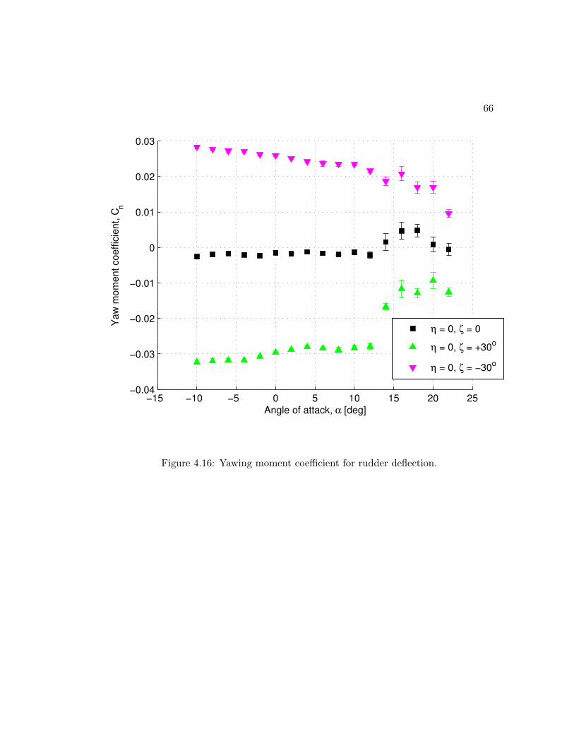
Figure 4.11 to Fig.4.16 show the experiment results for rudder deflection. This
rudder deflection will affect the side force balance. A positive rudder deflection gives
a positive side force and a negative the yawing moment of the aircraft as shown in
Fig. 4.12 and Fig. 4.16, respectively. The rudder deflection will not affect the lift
and pitching moment as the elevator does. The rudder effectiveness is affected by the
angle of attack. The frontal area seen by the airflow increases as the angle of attack
increases and this will block the airflow to flow through the rudder. The rudder becomes
dramatically less effective in the stall region as shown in Fig. 4.16. This set of data also
shows that the stall region begins at the angle of attack between 12◦ and 14◦.

61
−15 −10 −5 0 5 10 15 20 250
0.1
0.2
0.3
0.4
0.5
0.6
0.7
Angle of attack, α [deg]
Dra
g c
oeffic
ient, C
D
η = 0, ζ = 0
η = 0, ζ = +30o
η = 0, ζ = −30o
Figure 4.11: Drag coefficient for rudder deflection.

62
−15 −10 −5 0 5 10 15 20 25−0.2
−0.15
−0.1
−0.05
0
0.05
0.1
0.15
Angle of attack, α [deg]
Sid
e forc
e c
oeffic
ient, C
Y
η = 0, ζ = 0
η = 0, ζ = +30o
η = 0, ζ = −30o
Figure 4.12: Transverse force coefficient for rudder deflection.

63
−15 −10 −5 0 5 10 15 20 25−1
−0.5
0
0.5
1
1.5
Angle of attack, α [deg]
Lift coeffic
ient, C
L
η = 0, ζ = 0
η = 0, ζ = +30o
η = 0, ζ = −30o
Figure 4.13: Lift coefficient for rudder deflection.

64
−15 −10 −5 0 5 10 15 20 25−0.005
0
0.005
0.01
0.015
0.02
0.025
0.03
Angle of attack, α [deg]
Roll
mom
ent coeffic
ient, C
l
η = 0, ζ = 0
η = 0, ζ = +30o
η = 0, ζ = −30o
Figure 4.14: Rolling moment coefficient for rudder deflection.

65
−15 −10 −5 0 5 10 15 20 25−0.7
−0.6
−0.5
−0.4
−0.3
−0.2
−0.1
0
0.1
0.2
Angle of attack, α [deg]
Pic
th m
om
ent coeffic
ient, C
m
η = 0, ζ = 0
η = 0, ζ = +30o
η = 0, ζ = −30o
Figure 4.15: Pitching moment coefficient for rudder deflection.
66
−15 −10 −5 0 5 10 15 20 25−0.04
−0.03
−0.02
−0.01
0
0.01
0.02
0.03
Angle of attack, α [deg]
Yaw
mom
ent coeffic
ient, C
n
η = 0, ζ = 0
η = 0, ζ = +30o
η = 0, ζ = −30o
Figure 4.16: Yawing moment coefficient for rudder deflection.

Chapter 5
Conclusions and Future Work
5.1 Conclusions
This thesis has shown the result of propeller performance estimator and model of wind
tunnel uncertainties from a small UAV. The propeller performance estimator is based
on the Blade-element and Momentum theory with the induced angle of attack or the
induced velocity computed by combining the Goldstein’s vortex theory and Kutta-
Joukowski theorem. The stochastic model of propeller performance was developed by
perturbing the parameters which describe the operating conditions and propeller geome-
try. The objective was to see how the propeller performance is affected by the uncertain-
ties in velocity, RPM, propeller geometry and aerodynamics. The model of wind tunnel
uncertainties was developed based on the experiment of a small UAV (Mini-Ultrastick)
in wind tunnel. The objective of this experiment is to see how the uncertainties of the
aerodynamic coefficients varies with the angle of attack.
From the results of propeller performance prediction, the nominal performance result
agrees with the experimental result. In the stochastic model, the results showed that
in general the uncertainties in predicted thrust increases as the advance ratio increases.
The thrust and power coefficient uncertainties are proportional to the uncertainty of the
inputs. However, for the case where the lift curve slope was perturbed, the uncertainties
decreases and increases as the advance ratio varies from low to high.
In the wind tunnel experiment, the results showed that the uncertainties of the
aerodynamic coefficients can split into two regions, before stall (low angle of attack)
67

68
and after entering stall (high angle of attack) conditions. The angle of attack that splits
these two regions is between 12◦ and 14◦. The aerodynamic coefficient curves showed
that there is a discontinuity. The uncertainties are relatively small before stall and
become large after entering the stall region.
5.2 Future Work
The following is a list of some areas for future work:
1. Propeller blade’s physical measurement and its aerodynamics: Any pro-
peller has its own blade geometry description which includes chord length, thick-
ness, and pitch angle. The blade cross section is an airfoil and the blade will
produce lift and drag when the propeller is in operation. The information about
the blade geometry and its aerodynamics is crucial information in predicting the
propeller performance. However, determining or predicting this information for
any propeller is a hard problem unless the manufacturer provides one. It is very
difficult to do reverse engineering to get this information. A method for doing this
reverse engineering quickly will be beneficial.
2. Considering the effect of compressible flow: The propeller performance
results in this thesis ware computed by assuming that the airflow is incompress-
ible. The propeller blade sections near the tip normally or may operate at high
subsonic speed and the airflow at this condition violates the assumption of the
incompressible flow.
3. Considering multiple sources of uncertainties in the propeller perfor-
mance computation: The uncertainty analysis performed in this thesis only
looked at a single source of uncertainty.
4. Modeling the boundary layer of the wind tunnel: The result of the wind
tunnel experiment of a small did not take into account the effect of boundary
layer. The tunnel speed varies with the pitch angle or angle of attack.

References
[1] Hickman, M., P. Mirchandani, A. Angel and D. Chandnani, NCRST-F Year 1
Report. Project 3 - Needs Assessment and Allocation of Imaging Resources For
Transportation Planning and Management, ATLAS Research Center, University of
Arizona. Tucson, AZ, September 30, 2001.
[2] Gebre-Egziabher D., RPV/UAV Surveillance for Transportation Management and
Security, University of Minnesota Intelligent Transportation Systems Institute Re-
port CTS 08-27, Minneapolism MN, December 2008.
[3] Nonami, Kenzo, Modeling and Control of Unmanned Small Scale Rotorcraft UAVs
and MAVs, SpringerLink, London, 2010.
[4] Weibel, R. E., R. J. Hansman, Safety Considerations for Operation of Different
Classes of UAV’s in the NAS, AIAA paper 2004-6244. Proceedings of the Aviation
Technology, Integration and Operation (ATIO) Forum, Chicago, IL, September
2004.
[5] Weibel, R. E., R. J. Hansman, An Integrated Approach to Evaluating Risk Mitiga-
tion Measures for UAV Operational Concepts in the NAS, AIAA paper 2005-6957.
Proceedings of Infotech Aerospace Conference. Arlington, VA, September, 2005.
[6] Gebre-Egziabher D., Z. Xing, Analysis of Unmanned Aerial Vehicles Concepts of
Operations in ITS Applications, University of Minnesota Intelligent Transportation
Systems Institute Report CTS 11-05, Minneapolis, MN, December 2011.
[7] DATCOM, http://www.pdas.com/datcom.html
69

70
[8] Raymer, Daniel P., Aircraft Design: A Conceptual Approach, 3th ed., AIAA Edu-
cation Series, Virginia, 1999.
[9] Roskam, Jan, Aircraft Design, 3rd ed., DARcorporation, 2002.
[10] Watts, Henry C., The Design of Screw Propellers for Aircraft. Longmans, Green
and Co., New York, 1920.
[11] Theodorsen, Theodore, Theory of Propellers, McGraw-Hill Book Company, New
York, 1948.
[12] Weick, Fred. E., Aerodynamic tests were made with four geometrically similar metal
propellers of different diameters, National Advisory Committee for Aeronautics,
NACA TR No. 339, 1931.
[13] Weick, Fred. E., Full-scale wind-tunnel tests on several metal propellers having
different blade forms, National Advisory Committee for Aeronautics, NACA TR
No. 340, 1931.
[14] Freeman, Hugh B., Comparison of full-scale propellers having R.A.F.-6 and Clark
Y airfoil sections, National Advisory Committee for Aeronautics, NACA TR No.
378, 1932.
[15] Hartman, Edwin P., David Biermann, The aerodynamic characteristics of full-
scale propellers having 2, 3, and 4 blades of Clark y and R.A.F. 6 airfoil sections,
National Advisory Committee for Aeronautics, NACA TR No. 640, 1938.
[16] McCormick, Barnes W., Aerodynamics, Aeronautics and Flight Mechanics, 2nd ed.,
Wiley, New York, 1995.
[17] Wald, Quentin R., The Aerodynamics of Propellers, Progress in Aerospace Science
42, Elsevier, 2006 (pages 85 - 128).
[18] Adkins, Charles N., Robert H. Liebeck, Design of Optimum Propeller, Jounal of
Propulsion and Power, Vol. 10, No. 15, Sept. - Oct. 1994.
71
[19] Owens, D. Bruce, David E. Cox, Eugene A. Morelli, Development of a Low-Cost
Sub-Scale Aircraft for Flight Research: The FASER Project, 25th AIAA Aerody-
namic Measurement Technology and Ground Testing Conference, AIAA 2006-3306,
San Francisco, California, June 2006.
[20] Mises, R., Theory of Flight. Dover, New York, 1945.
[21] Weick, Fred E., Aircraft Propeller Design. McGraw Hill, New York, 1930.
[22] Corson, Blake W., A Review of Propeller Theory, NACA: Univ. Conf. on Aerodyn.,
Jan 1, 1948.
[23] Bertin, John J. and Micheal L. Smith, Aerodynamics for Engineers, 3rd ed.,
Prentice-Hall Inc., New Jersey, 1998.
[24] Anderson, John D., Fundamental of Aerodynamics, 4th ed., McGraw-Hill, New
York, 2007.
[25] Wind Tunnel of the Department of Aerospace Engineering and Mechanics, Univer-
sity of Minnesota, http://www.aem.umn.edu/facilities/windtunnel/
[26] APC Propellers (personal communication, April 5, 2011) http://www.apcprop.
com
[27] Selig, Micheal S. and Gavin Ananda, Low Reynolds Number Propeller Perfor-
mance Data: Wind Tunnel Corrections for Motor Fixture Drag, University of
Illinois at Urbana-Champaign, 2011. http://www.ae.illinois.edu/m-selig/
props/uiuc-props-wind-tunnel-correction.pdf

Appendix A
Nomenclature
A Actuator disc area
B Number of propeller blades
C1 Total pressure in front of actuator disc
C2 Total pressure in behind of actuator disc
CD Drag coefficient
CL Lift coefficient
CLα Lift curve slope
CP Power coefficient
CQ Torque coefficient
CT Thrust coefficient
CY Side force coefficient
Cdf Fixture drag coefficient
Cl Rolling moment coefficient
Cm Pitching moment coefficient
Cn Yawing moment coefficient
D Propeller diameter, Drag force (aircraft)
F Prandtl’s tip loss factor
FX Axial force
FY Transverse force
FZ Normal force
Fd Fixture drag force
72

73
J Advance ratio
L Lift force
Lcg Rolling moment about cg location
MX Axial moment
Mcg Pitching moment about cg location
MY Transverse moment
MZ Normal moment
Ncg Yawing moment about cg location
P Propeller Power
Pi Propeller induced power
Po Propeller thrust power
Q Propeller torque
Sw Aircraft’s wing area
T Propeller thrust
V Forward velocity
VE Effective velocity =√V 2R + w2
VR Resultant velocity =√
(ωr)2 + V 2
VT Blade tip velocity
Y Side force
b Sectional blade chord length
bw Aircraft’s wing span
cw Aircraft’s wing chord length
dD Differential drag force
dFQ Differential torque force
dL Differential lift force
dT Differential thrust
dp Air pressure increment behind actuator disc
dr Radial increment length of propeller blade
f(α) Function describes mathematical model of lift curve
h Sectional blade thickness
m Mass flow rate
p Air pressure far from actuator disc
74
p′ Air pressure at the actuator disc
p Propeller pitch
r Sectional blade radius
w Induced velocity at actuator disc or propeller blade
w′ Induced velocity far behind actuator disc
wa Axial component of induced velocity
wt Tangential component of induced velocity
x Normalized sectional blade radius
xT Normalized propeller tip radius
xcg Distance between cg location and measurement point projected along x-body axis
xh Normalized propeller hub radius
zcg Distance between cg location and measurement point projected along z-body axis
∆α Angle of attack correction
∆cL Lift coefficient correction
∆θ Correction factor due to tangential induced velocity
Γ Bound vortex circulation
α Angle of attack
αi Induced angle of attack
β Sectional blade angle
η Efficiency
ηi Ideal efficiency (Momentum theory)
κ Goldstein’s circulation factor
λ Local advance ratio
φ Flow angle
ρ Air density
σ Sectional blade solidity
σ[•] Standard deviation
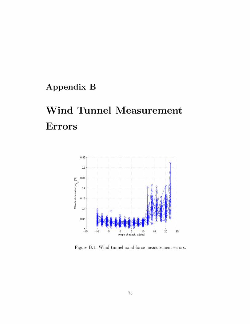
Appendix B
Wind Tunnel Measurement
Errors
−15 −10 −5 0 5 10 15 20 250
0.05
0.1
0.15
0.2
0.25
0.3
0.35
Angle of attack, α [deg]
Sta
ndard
devia
tion,
σF
X
[N
]
Figure B.1: Wind tunnel axial force measurement errors.
75
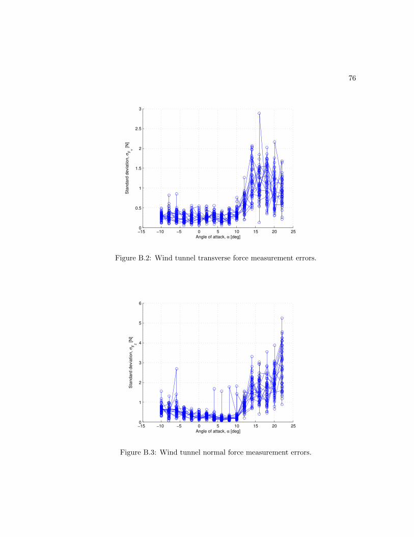
76
−15 −10 −5 0 5 10 15 20 250
0.5
1
1.5
2
2.5
3
Angle of attack, α [deg]
Sta
ndard
devia
tion,
σF
Y
[N
]
Figure B.2: Wind tunnel transverse force measurement errors.
−15 −10 −5 0 5 10 15 20 250
1
2
3
4
5
6
Angle of attack, α [deg]
Sta
ndard
devia
tion,
σF
Z
[N
]
Figure B.3: Wind tunnel normal force measurement errors.
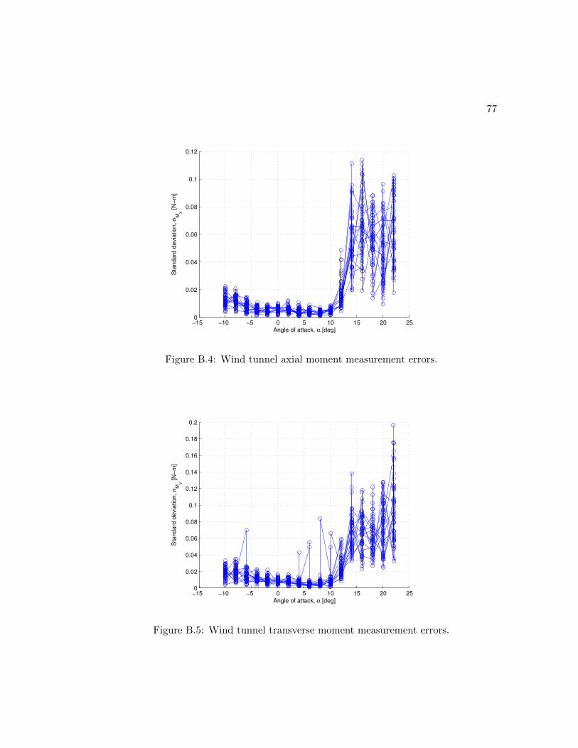
77
−15 −10 −5 0 5 10 15 20 250
0.02
0.04
0.06
0.08
0.1
0.12
Angle of attack, α [deg]
Sta
ndard
devia
tion,
σM
X
[N
−m
]
Figure B.4: Wind tunnel axial moment measurement errors.
−15 −10 −5 0 5 10 15 20 250
0.02
0.04
0.06
0.08
0.1
0.12
0.14
0.16
0.18
0.2
Angle of attack, α [deg]
Sta
ndard
devia
tion,
σM
Y
[N
−m
]
Figure B.5: Wind tunnel transverse moment measurement errors.

78
−15 −10 −5 0 5 10 15 20 250
0.01
0.02
0.03
0.04
0.05
0.06
0.07
Angle of attack, α [deg]
Sta
ndard
devia
tion,
σM
Z
[N
−m
]
Figure B.6: Wind tunnel normal moment measurement errors.