Essays on terms of trade

A DISSERTATIONSUBMITTED TO THE FACULTY OF THE GRADUATE SCHOOL

OF THE UNIVERSITY OF MINNESOTABY

Jorge Mondragon Minero

IN PARTIAL FULFILLMENT OF THE REQUIREMENTSFOR THE DEGREE OF

DOCTOR OF PHILOSOPHY

Manuel Amador, AdvisorTimothy J. Kehoe, Co-Advisor

August, 2019

c©Jorge Mondragon Minero 2019ALL RIGHTS RESERVED

Acknowledgements

I would like to express how grateful I am to my advisors Manuel Amador,Timothy Kehoe, and Javier Bianchi. Undoubtedly my work and studies reflecttheir guidance and mentoring. I am also grateful to my colleagues in the tradeworkshop at the University of Minnesota for their help and insight during dis-cussions inside and outside the classroom. In particular, I would like to thankVegard Nygard, Sora Lee, and Jarek Strzalkowski for their companionship andfriendship throughout my studies. Finally, but not least, I would like to thankmy family and friends for their constant support and love.

ii

Dedication

To my mother and grandmother. Thank you for always believing in me.

..no tenemos saca

iii

iv

Abstract

This dissertation consists of three chapters. The main topic I study throughthem is fluctuations in terms of trade and their effects in small open economies.In particular, I study their effects in the labor and financial markets.

In Chapter 1, I study the how the labor market and real GDP interact tofluctuations in the terms of trade. Conventional wisdom suggests that whenterms of trade deteriorate in small open economies, real GDP decreases. Inthis paper, I document that the correlation between terms of trade and realGDP innovations varies widely between both positive and negative values acrossdifferent countries. Furthermore, I show that this variation cannot be explainedby income alone. This raises the question, why do countries’ real GDPs reactdifferently toward changes in their terms of trade? I show evidence that theway in which countries react toward changes in terms of trade is linked to thelabor market. I build a real business cycle model in which a small open economyexperiences terms of trade fluctuations in conjunction with real wage rigidity. Ifind that an economy with a real wage rigidity is able to produce either a positiveor a negative correlation between terms of trade and real GDP innovations.

In Chapter 2, Sora Lee and I study the relationship between terms of tradefluctuations and changes in the sovereign government interest rate spreads inemerging economies. We propose a stochastic general equilibrium model ofsovereign default with endogenous default risk in order to explain the interestrate behavior in emerging economies. We incorporate two types of shocks tocover a foreign and a domestic uncertainty. We define as the domestic and theforeign uncertainty, GDP and terms of trade shock, respectively. The model isable to successfully increase the dispersion of sovereign interest rates when GDP

v

shocks are above the trend. This result seems to suggest that terms of trade is agood candidate to explain the volatility of interest rates in small open economieswhen they are not under recessions or crises.

In Chapter 3, I study the optimal choice of foreign issued debt incurred bya sovereign government in a small open economy. In particular, what are theshortcomings and benefits from issuing debt in a currency tightly linked to atrade partner country. I propose a two period model with uncertainty in theterms of trade and in a real exchange rate to show the benefits and costs. I findthat when a government is in a deep recession, issuing debt in a currency that isnot tightly linked to their trade becomes optimal.

Contents

Acknowledgments ii

Dedication iii

Abstract v

List of tables ix

List of figures 1

1 Terms of trade and unemployment in the business cycle 11.1 Introduction . . . . . . . . . . . . . . . . . . . . . . . . . . . . . . 11.2 Kehoe-Ruhl Observation . . . . . . . . . . . . . . . . . . . . . . . 3

1.2.1 Standard Model . . . . . . . . . . . . . . . . . . . . . . . . 41.2.2 Wage Rigidity Mechanism . . . . . . . . . . . . . . . . . . 7

1.3 Empirical Analysis . . . . . . . . . . . . . . . . . . . . . . . . . . 91.3.1 Real Wage Rigidity . . . . . . . . . . . . . . . . . . . . . . 13

1.4 Model . . . . . . . . . . . . . . . . . . . . . . . . . . . . . . . . . 151.4.1 Households . . . . . . . . . . . . . . . . . . . . . . . . . . 16

vi

vii

1.4.2 Representative Final Good Firm . . . . . . . . . . . . . . . 171.4.3 Labor Market & Unemployment . . . . . . . . . . . . . . . 181.4.4 Unemployment Mechanism . . . . . . . . . . . . . . . . . . 191.4.5 Recursive Characterization . . . . . . . . . . . . . . . . . . 20

1.5 Quantitative Analysis . . . . . . . . . . . . . . . . . . . . . . . . . 231.5.1 Baseline Calibration . . . . . . . . . . . . . . . . . . . . . 23

1.6 Conclusion . . . . . . . . . . . . . . . . . . . . . . . . . . . . . . . 29

2 Sovereign spread movements in emerging economies: terms oftrade matter 342.1 Introduction . . . . . . . . . . . . . . . . . . . . . . . . . . . . . . 342.2 Empirical evidence . . . . . . . . . . . . . . . . . . . . . . . . . . 38

2.2.1 Currency composition of sovereign external debt . . . . . . 382.3 Terms of trade, GDP and spread across countries . . . . . . . . . 432.4 Model . . . . . . . . . . . . . . . . . . . . . . . . . . . . . . . . . 45

2.4.1 Recursive Equilibrium . . . . . . . . . . . . . . . . . . . . 522.4.2 Aggregate Recursive Equilibrium . . . . . . . . . . . . . . 572.4.3 No Persistency Case . . . . . . . . . . . . . . . . . . . . . 61

2.5 Quantitative analysis . . . . . . . . . . . . . . . . . . . . . . . . . 632.5.1 Data . . . . . . . . . . . . . . . . . . . . . . . . . . . . . . 632.5.2 Calibration . . . . . . . . . . . . . . . . . . . . . . . . . . 652.5.3 Results . . . . . . . . . . . . . . . . . . . . . . . . . . . . . 70

2.6 Conclusion . . . . . . . . . . . . . . . . . . . . . . . . . . . . . . . 73

3 Optimal foreign currency debt denomination 753.1 Introduction . . . . . . . . . . . . . . . . . . . . . . . . . . . . . . 75

viii

3.2 Two Period Model . . . . . . . . . . . . . . . . . . . . . . . . . . 763.2.1 Representative Household . . . . . . . . . . . . . . . . . . 763.2.2 Representative Firm . . . . . . . . . . . . . . . . . . . . . 773.2.3 Foreign International Lenders . . . . . . . . . . . . . . . . 783.2.4 Benevolent Government . . . . . . . . . . . . . . . . . . . 783.2.5 Equilibrium . . . . . . . . . . . . . . . . . . . . . . . . . . 80

3.3 Quantitative Analysis . . . . . . . . . . . . . . . . . . . . . . . . . 833.3.1 Baseline Calibration . . . . . . . . . . . . . . . . . . . . . 84

3.4 Conclusion . . . . . . . . . . . . . . . . . . . . . . . . . . . . . . . 86

Bibliography 92

4 Appendix 934.1 Propositions proofs . . . . . . . . . . . . . . . . . . . . . . . . . . 94

4.1.1 Proposition 4 (Recursive Equilibrium Isomorphism) . . . . 944.1.2 Proposition 5 (Default Sets Monotonicity) . . . . . . . . . 964.1.3 Proposition 6 (No Resources Inflows) . . . . . . . . . . . . 974.1.4 Proposition 7 (GDP Default Incentives) . . . . . . . . . . 984.1.5 Proposition 8 (Terms of Trade Default Incentives) . . . . . 100

4.2 Computational algorithm . . . . . . . . . . . . . . . . . . . . . . . 104

List of Tables

1.1 Sample classification of countries by income . . . . . . . . . . . . 101.2 Terms of trade residuals autorgressive analysis . . . . . . . . . . . 121.3 Terms of trade and macroeconomic indicators correlations . . . . 121.4 Calibration table . . . . . . . . . . . . . . . . . . . . . . . . . . . 271.5 Parameter Values . . . . . . . . . . . . . . . . . . . . . . . . . . . 28

2.1 Foreign Currency Debt Composition . . . . . . . . . . . . . . . . 412.2 Descriptive Statistics in Emerging Economies . . . . . . . . . . . 462.3 Correlations in Emerging Economies . . . . . . . . . . . . . . . . 472.4 Business Cycles Statistics for Mexico . . . . . . . . . . . . . . . . 642.5 Parameters Specification . . . . . . . . . . . . . . . . . . . . . . . 692.6 Model Business Cycles Statistics . . . . . . . . . . . . . . . . . . . 72

3.1 Calibration table . . . . . . . . . . . . . . . . . . . . . . . . . . . 85

ix

List of Figures

1.1 Closed form solution real GDP from deterministic example . . . . 81.2 Relationship between terms of trade fluctuations, real GDP, and

the labor market . . . . . . . . . . . . . . . . . . . . . . . . . . . 141.3 Ecuador and Greece correlation between terms of trade and real

GDP . . . . . . . . . . . . . . . . . . . . . . . . . . . . . . . . . . 151.4 Representation of a negative terms of trade shock . . . . . . . . . 311.5 Relationship between correlation of real GDP and terms of trade

residuals and correlation of employment and terms of trade . . . . 321.6 Relationship between correlation of real GDP and terms of trade

residuals and correlation of unemployment rates and terms of trade 33

2.1 Spreads and Cyclical Components in Mexico . . . . . . . . . . . . 352.2 Foreign Debt Profile for Emerging Economies . . . . . . . . . . . 432.3 Default Set Boundaries . . . . . . . . . . . . . . . . . . . . . . . . 712.4 Sovereign Bond Pricing and Sovereign Interest Rate . . . . . . . . 72

3.1 Debt pricing and second period discounted expected value contin-gent in debt . . . . . . . . . . . . . . . . . . . . . . . . . . . . . . 82

3.2 Optimal debt issuance contingent to initial debt . . . . . . . . . . 86

x

Chapter 1

Terms of trade andunemployment in the businesscycle

1.1 Introduction

Conventional wisdom suggests that when terms of trade deteriorate, smallopen economies are negatively affected. This deterioration implies a contractionof available resources. Thus, the country becomes poorer, making macroeconomicindicators such as real GDP fall. This notion is summarized in Easterly, Islam andStiglitz (2001) which states, "For small open economies, adverse terms of tradeshocks can have much the same effect as negative technology shocks, and this isone of the important differences between macroeconomics in these economies andthat which underlies some of the traditional closed economy models."

1

2

In this paper, I argue that the conventional narrative regarding terms of tradeis not entirely consistent with the data. I document that the shock correlationbetween terms of trade and real GDP varies widely between positive and nega-tive values across 122 countries. Furthermore, this variation is not explained byincome levels alone. This raises the question, why do countries react differentlytoward terms of trade shocks? I show evidence that the way in which countriesreact toward terms of trade shocks is linked to their labor markets. Specifically,when unemployment reacts positively to increases in the terms of trade, real GDPreacts negatively.

Modeling the relationship between real GDP and terms of trade is not trivial.Kehoe and Ruhl (2008) show that standard models fail to generate a negativecorrelation between terms of trade and real GDP innovations. This is becausean economy becomes poorer when facing an adverse terms of trade shock. Withstandard elasticities, this increases employment, and, as a result, real GDP in-creases. Because conventional wisdom suggests small open economies are neg-atively affected by deteriorating terms of trade, the literature has only focusedon addressing what type of assumptions or frictions generate this negative rela-tion. In this paper, I propose a mechanism that is able to account for not onlya negative, but also a positive correlation between terms of trade and real GDPinnovations. I build a real business cycle model in which a small open economyexperiences terms of trade fluctuations in conjunction with real wage rigidity.

The model illustrates how the effect of an adverse terms of trade shock onlabor and real GDP in a small open economy is determined by whether or notthe real wage rigidity is binding. Given an adverse terms of trade shock, if thereal wage rigidity does not bind, labor and real GDP increase in equilibrium.On the other hand, when the real wage rigidity does bind, firms hire less labor,

3

increasing unemployment and decreasing labor and real GDP.

1.2 Kehoe-Ruhl Observation

It has been of particular interest to study how terms of trade influence smallopen economies. Mendoza (1995) finds that terms of trade shocks1 tend to belarge, persistent, and weakly procyclical accounting for nearly half of real GDPfluctuations. Moreover, in Mendoza (1997) states that for industrial and devel-oping countries, volatility in the terms of trade has a large and adverse effect oneconomic growth. Expanding to these results, Kose (2002) finds that interna-tional prices fluctuations are the main driver of economic volatility in developingeconomies. One of the main sources of influence terms of trade affect an economyis via the exchange rates. In De Gregorio and Wolf (1994) show that the realexchange rate fluctuations is mainly driven by the volatility of the terms of trade.Expanding to this notion, Broda (2004) shows that countries with fixed exchangerate regimes experience larger contractions in real GDP.

The highlighted relationship between terms of trade changes and movementsin real GDP is difficult to replicate theoretically though. Conventional wisdomsuggests that real GDP should fall after a terms of trade deterioration. Thiswas challenged in Kehoe and Ruhl (2008) by explaing why standard models withterms of trade shocks fail to generate changes in real GDP consistent with thedata. There are ways to enrich the standard model to replicate falls in real GDPdue to terms of trade deteriorations. Using Greenwood-Hercowitz-Huffman pref-

1In this paper, terms of trade is defined as the ratio of export to import unit values, mea-suring at constant import prices. In this sense, a deterioration of the terms of trade will bereflected as a fall in the terms of trade.

4

erences solve the issues because wealth effects are unexistant. In this way, whenhaving negative terms of trade shocks, households are not willing to supply morelabor even though they become poorer. Another way, de Soyres (2016) proposes amodel with monopolistic competition and love for variety to generate falls in realGDP via contractions in producers profits when terms of trade deteriorate. Also,Costa (2017) proposes a model where natural resources are taken into consider-ation in the household preferences, generating falls in real GDP when terms oftrade deteriorate due to idle resources. Finally, Benguria, Saffie and Urzúa (2018)uses a downward nominal rigidity and a fixed exchange rate regime to generatecontractions in real GDP via falls in international prices when the rigidity binds.

In this paper I explore deeper this last mechanism. Specifically, I focus inthe ability for wage rigidities to create opposite effects in real GDP for the samechange in the terms of trade. To understand better this observation, let meillustrate it with a simple example.

1.2.1 Standard Model

Consider a production function F (·, ·, ·) owned by a representative firm thattakes as inputs capital K, labor L, and foreign intermediate inputs M , satisfyingINADA conditions. Let the technology be indexed by z, a productivity parame-ter. The firm rents capital at a price r, hires labor at a wage w, and buys foreignintermediate inputs at a price p. The price of p will represent the terms of trade.

5

Then, the representative firm’s profit maximization problem is

MaxY,K,L,M

{Y − rK − wL− pM}

s.t. Y ≤ zF (K,L,M)

Y,K,L,M ≥ 0

This yields the following first order conditions,

r(p) = z∂F

∂K

(K(p), L(p), M(p)

), w(p) = z

∂F

∂L

(K(p), L(p), M(p)

),

and p = z∂F

∂M

(K(p), L(p), M(p)

).

Here, K(p) the optimal amount of capital stock rented, L(p) the optimal amountof labor hired, and M(p) the optimal amount of foreign intermediate inputsbought. Also, r(p) the equilibrium return to capital and w(p) the equilibriumreal wage. Now, let us compute real GDP taking p0 > 0 as the base year price,

GDP (p) ≡ Y (p)− p0M(p) = zF (K(p), L(p), M(p))− p0M(p).

Notice that to compute real GDP, a base year price must be used. Computingthe derivative with respect of terms of trade, we find that

GDP ′(p) = z∂F

∂L

(K(p), L(p), M(p)

)K ′(p) + z

∂F

∂L

(K(p), L(p), M(p)

)L′(p)

+ z∂F

∂M

(K(p), L(p), M(p)

)M ′(p)− p0M

′(p)

= r(p)K ′(p) + w(p)L′(p) + (p− p0) M ′(p).

6

Now, note that the capital stock is a decision settled in the previous period,K(p) = K. This is, the realization of current terms of trade p only has theinfluence in the next period’s capital stock. Therefore, current equilibrium capitalstock does not change with how the realization of terms of trade, K ′(p) = 0. Also,if changes in the terms of trade p are small and around the base year p0, then wehave that p ≈ p0. Therefore, the terms of trade first order effects in real GDPcan be approximated as

GDP ′(p) ≈ w(p)L′(p). (1.1)

With an inelastic supply of labor L = L, the optimal amount of labor is fixedregardless of the terms of trade, and thus L′(p) = 0. Nevertheless, when relaxingthis assumption, the optimal labor can change. Specifically, the optimal laborchanges because the terms of trade changes the equilibrium real wage. For stan-dard production functions, it is normal to find that real wages fall when thereis a deterioration of the terms of trade, w′(p) < 0. In addition, for standardelasticity of substitutions from the household preferences between consumptionand leisure, it is common to find L′(p) > 0. This is, labor increases in equilibriumfor an increase in the terms of trade because households become poorer due tothe fall in real wages. In other words, changes in the real GDP do not move inthe opposite direction to the changes in the terms of trade because GDP ′(p) ≥ 0.This is the Kehoe-Ruhl observation, standard models are unable to replicate thenegative relationship between changes in real GDP and changes in terms of tradethat the data shows for some countries.

7

1.2.2 Wage Rigidity Mechanism

Now, let us assume there is a friction in the labor market, the real wage cannotfall lower than w > 0. When the equilibrium real wage is such that w(p) ≥ w,then real GDP and labor behaves the same way as the frictionless environmentdescribed in the previous subsection. Nonetheless, this relationship changes whenthe real wage rigidity binds. When the real wage rigidity binds, the equilibriumreal wage is fixed, w(p) = w. Using the first order conditions for labor andforeign intermediate inputs and fixing the equilibrium current capital stock levelto K(p) = K, the following relationship holds

L′(p) =p ∂2F

∂L∂M

(K, L(p), M(p)

)− w ∂2F

∂M2

(K, L(p), M(p)

)w ∂2F∂M∂L

(K, L(p), M(p)

)− p∂2F

∂L2

(K, L(p), M(p)

) M ′(p).

Because the production function F (·, ·, ·) satisfies the INADA conditions, we knowthat ∂2F

∂L2 , ∂2F∂M2 < 0 and ∂2F

∂L∂M, ∂2F∂M∂L

> 0. Therefore, how the optimal demandof labor reacts towards terms of trade shares the same direction as how optimalforeign intermediate inputs react to terms of trade. In addition, with standardelasticities of substitution in the production function, the optimal foreign inter-mediate inputs react negatively towards terms of trade, M ′(p) < 0. When thereal wage rigidity is binding, the equilibrium labor is demand determined. There-fore, because households are not in their labor supply curve, the equilibrium laborfalls when terms of trade deteriorate. Furthermore, the household preferences willdefine a gap between the equilibrium labor and the desired labor supplied in theeconomy. This disparity describes the unvoluntary unemployment in equilibrium.Because equation (1.1) holds as well in this case, real GDP decreases when termsof trade deteriorate.

8

(a) Low real wage rigidity

Terms of trade0.6 0.8 1.0 1.2 1.4

20%

40%

60%

80%

100%

ConstrainedUnconstrained

p0

Real Wage Rigidity

Perfectly Flexible

(b) High real wage rigidity

Terms of trade0.6 0.8 1.0 1.2 1.4

20%

40%

60%

80%

100%

ConstrainedUnconstrained

p0

Real Wage Rigidity

Perfectly Flexible

Figure 1.1: Closed form solution real GDP from deterministic example

Note: Deterministic example solution for real GDP using the following parameters: αK =0.10, αL = 0.45, αM = 0.45, K = 1, L = 1.00, z = 1.00, p0 = 1.00, wlow = 0.2017, andwhigh = 0.2812. The two real wage rigidities were picked so the real wage constraint becomesbinding at ±0.20% from the base terms of trade price p0. The real GDP is deflated level isdeflated by the real GDP obtained when there is no real wage rigidity and the terms of tradeis at base p0 = 1.

Figure 1.1 illustrates how the mechanism affect real GDP. I assume a constantreturns to scale production function F (K,L,M) = KαKLαLMαM and an inelasticlabor supply of labor L. Both figures show with a dashed line how real GDPmoves as terms of trade changes in a frictionless environment. The importantthing to notice is that at the base price terms of trade, the slope of real GDP iszero. In other words, relatively small changes around the base year terms of tradeyield approximately no changes in real GDP. Panel 1.1(a) shows what happenswhen there is a low real wage rigidity. In this case, small changes in the terms oftrade around the base year give the same results as the frictionless case. In other

9

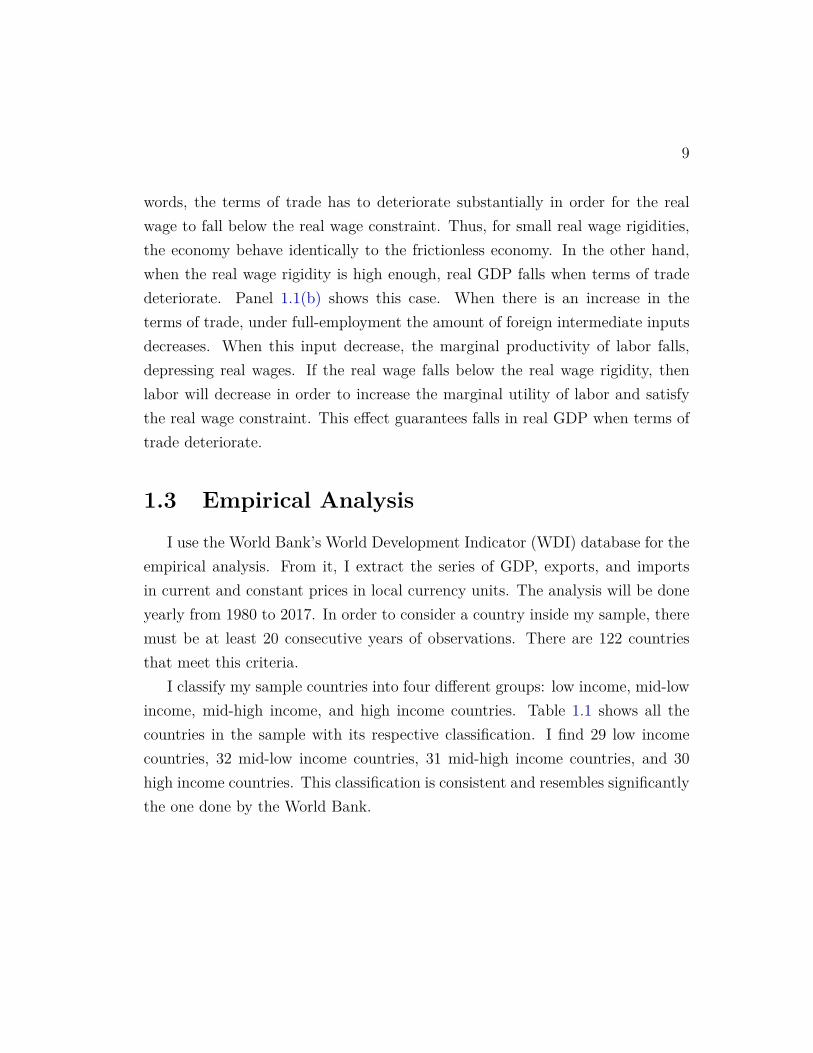
words, the terms of trade has to deteriorate substantially in order for the realwage to fall below the real wage constraint. Thus, for small real wage rigidities,the economy behave identically to the frictionless economy. In the other hand,when the real wage rigidity is high enough, real GDP falls when terms of tradedeteriorate. Panel 1.1(b) shows this case. When there is an increase in theterms of trade, under full-employment the amount of foreign intermediate inputsdecreases. When this input decrease, the marginal productivity of labor falls,depressing real wages. If the real wage falls below the real wage rigidity, thenlabor will decrease in order to increase the marginal utility of labor and satisfythe real wage constraint. This effect guarantees falls in real GDP when terms oftrade deteriorate.

1.3 Empirical Analysis

I use the World Bank’s World Development Indicator (WDI) database for theempirical analysis. From it, I extract the series of GDP, exports, and importsin current and constant prices in local currency units. The analysis will be doneyearly from 1980 to 2017. In order to consider a country inside my sample, theremust be at least 20 consecutive years of observations. There are 122 countriesthat meet this criteria.

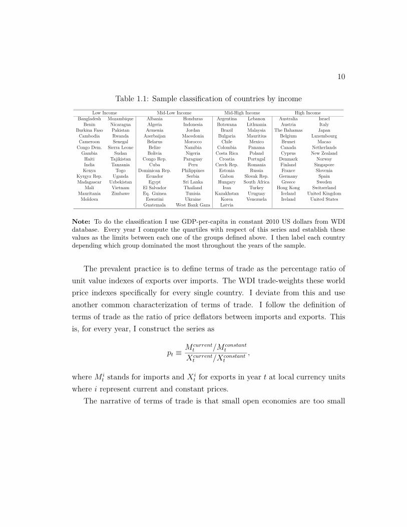
I classify my sample countries into four different groups: low income, mid-lowincome, mid-high income, and high income countries. Table 1.1 shows all thecountries in the sample with its respective classification. I find 29 low incomecountries, 32 mid-low income countries, 31 mid-high income countries, and 30high income countries. This classification is consistent and resembles significantlythe one done by the World Bank.

10

Table 1.1: Sample classification of countries by incomeLow Income Mid-Low Income Mid-High Income High Income

Bangladesh Mozambique Albania Honduras Argentina Lebanon Australia IsraelBenin Nicaragua Algeria Indonesia Botswana Lithuania Austria Italy

Burkina Faso Pakistan Armenia Jordan Brazil Malaysia The Bahamas JapanCambodia Rwanda Azerbaijan Macedonia Bulgaria Mauritius Belgium LuxembourgCameroon Senegal Belarus Morocco Chile Mexico Brunei MacaoCongo Dem. Sierra Leone Belize Namibia Colombia Panama Canada Netherlands

Gambia Sudan Bolivia Nigeria Costa Rica Poland Cyprus New ZealandHaiti Tajikistan Congo Rep. Paraguay Croatia Portugal Denmark NorwayIndia Tanzania Cuba Peru Czech Rep. Romania Finland SingaporeKenya Togo Dominican Rep. Philippines Estonia Russia France Slovenia

Kyrgyz Rep. Uganda Ecuador Serbia Gabon Slovak Rep. Germany SpainMadagascar Uzbekistan Egypt Sri Lanka Hungary South Africa Greece Sweden

Mali Vietnam El Salvador Thailand Iran Turkey Hong Kong SwitzerlandMauritania Zimbawe Eq. Guinea Tunisia Kazakhstan Uruguay Iceland United KingdomMoldova Eswatini Ukraine Korea Venezuela Ireland United States

Guatemala West Bank Gaza Latvia

Note: To do the classification I use GDP-per-capita in constant 2010 US dollars from WDIdatabase. Every year I compute the quartiles with respect of this series and establish thesevalues as the limits between each one of the groups defined above. I then label each countrydepending which group dominated the most throughout the years of the sample.

The prevalent practice is to define terms of trade as the percentage ratio ofunit value indexes of exports over imports. The WDI trade-weights these worldprice indexes specifically for every single country. I deviate from this and useanother common characterization of terms of trade. I follow the definition ofterms of trade as the ratio of price deflators between imports and exports. Thisis, for every year, I construct the series as

pt ≡M current

t /M constantt

Xcurrentt /Xconstant

t

,

where M it stands for imports and X i

t for exports in year t at local currency unitswhere i represent current and constant prices.

The narrative of terms of trade is that small open economies are too small

11

to offset the aggregate world supply and demand of the product they trade. Inother words, small open economies take as given international prices. Under thatnarrative, it is common to assume that terms of trade shocks of every countryfollow an AR(1) process independent from its macroeconomic indicators. Toobtain the terms of trade shocks, I take an HP-filter with a smoothing parameterof 100 to its log-series. Let pt represent the residuals between the original log-series and its trend. I consider the following process for terms of trade in everycountry

pt+1 = ρppt + σpεt+1, where ε ∼ N(0, 1).

Table 1.2 shows the average of the autoregressive analysis of terms of trade resid-uals. The average autocorrelation for all the countries in our sample is 0.339.For high income countries, terms of trade shock tend to be a bit more persistentcompared to mid-low and mid-high income countries. This value tells us thatterms of trade shocks die quickly. In the literature, a standard value for thisparameter is around 0.50. Using log-quadratic detrending recovers this value.Another feature of the analysis is that the volatility of the terms of trade shocksdecreases as we move across groups with higher income. The volatility excludinghigh income countries is around 7.57%, a standard deviation consistent with theliterature.

We now include other macroeconomic aggregate variables and see how termsof trade correlates with them. Table 1.3 shows the log-series HP-filter residualsusing the same smoothing parameter as before. Let us start with how termsof trade correlates with real GDP. For low income, mid-low income, and highincome countries, the correlation of real GDP is close to zero. Nevertheless, we

12

Table 1.2: Terms of trade residuals autorgressive analysis

Terms of Trade Low Mid-Low Mid-High High AllAR(1) Income Income Income Income Countriesρp 0.291 0.322 0.339 0.404 0.339σp 0.096 0.075 0.056 0.027 0.063R2p 0.148 0.145 0.157 0.192 0.160

find a negative relationship of -0.164 for mid-high income countries. This valueis consistent with the latest studies done for emerging economies. In the otherhand, there is a small negative relationship of 0.016% for high income countries.Another feature we find is that for high income countries, investment does notcorrelate with investment series. Nevertheless, for the rest of the countries, thereis a marked negative relationship between these two variables.

Table 1.3: Terms of trade and macroeconomic indicators correlations

Correlations with Low Mid-Low Mid-High High AllTerms of Trade Income Income Income Income Countries

GDP -0.071 0.047 -0.164 -0.016 -0.050C -0.141 -0.044 -0.244 -0.147 -0.143I -0.261 -0.081 -0.218 -0.131 -0.170NX -0.279 -0.362 -0.123 -0.175 -0.236L 0.070 -0.069 -0.098 -0.104 -0.052U -0.054 0.016 0.133 0.082 0.045

Figure 1.2 shows what in the data (1.1) represent for all the countries inthe sample. Realize that the variation among countries in how terms of tradecorrelate real GDP and labor2 related variables is diverse. Focus in Panel 1.2(a)

2The variables I consider are employment-popluation ratio and unemployment rate. I con-

13

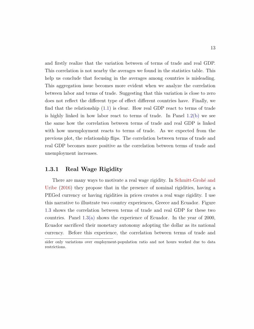
and firstly realize that the variation between of terms of trade and real GDP.This correlation is not nearby the averages we found in the statistics table. Thishelp us conclude that focusing in the averages among countries is misleading.This aggregation issue becomes more evident when we analyze the correlationbetween labor and terms of trade. Suggesting that this variation is close to zerodoes not reflect the different type of effect different countries have. Finally, wefind that the relationship (1.1) is clear. How real GDP react to terms of tradeis highly linked in how labor react to terms of trade. In Panel 1.2(b) we seethe same how the correlation between terms of trade and real GDP is linkedwith how unemployment reacts to terms of trade. As we expected from theprevious plot, the relationship flips. The correlation between terms of trade andreal GDP becomes more positive as the correlation between terms of trade andunemployment increases.

1.3.1 Real Wage Rigidity

There are many ways to motivate a real wage rigidity. In Schmitt-Grohé andUribe (2016) they propose that in the presence of nominal rigidities, having aPEGed currency or having rigidities in prices creates a real wage rigidity. I usethis narrative to illustrate two country experiences, Greece and Ecuador. Figure1.3 shows the correlation between terms of trade and real GDP for these twocountries. Panel 1.3(a) shows the experience of Ecuador. In the year of 2000,Ecuador sacrificed their monetary autonomy adopting the dollar as its nationalcurrency. Before this experience, the correlation between terms of trade and

sider only variations over employment-population ratio and not hours worked due to datarestrictions.

14

(a) Employment rate

-1.00 -0.75 -0.50 -0.25 0.00 0.25 0.50 0.75 1.00

-1.00

-0.75

-0.50

-0.25

0.00

0.25

0.50

0.75

1.00

ALB

DZA

ARG

ARM

AUS

AUT

AZEBHS

BGD

BLR

BEL

BLZ

BEN

BOL

BWA

BRA

BRNBGR

BFA

KHM

CMR

CAN

CHL

COL

COD

COG CRI

HRV

CUBCYP CZE

DNK

DOM

ECU

EGY

SLV

GNQ

EST

SWZ

FIN

FRAGABGMB

DEU

GRC

GTM

HTI

HND

HKG

HUN

ISL

IND

IDN

IRN

IRL

ISR

ITA

JAP

JOR

KAZ

KEN

KOR KGZ

LVA

LBN

LTU

LUX

MACMKD

MDG

MYS

MLI MRT

MUS

MEX

MDA

MAR

MOZ

NAM

NLDNZL NIC

NGA

NOR

PAKPAN

PRY

PER

PHL

POL

PORROU

RUS

RWA

SEN

SRB

SLE

SGP

SVK

SVN

ZAF

ESP

LKA

SDN

SWE

CHE

TJK

TZA

THATGO

TUN TUR

UGA

UKR

GBR USA

URY

UZB

VEN

VNM

PSE

ZWE

Correlation between terms of trade & employment

Correlationbetweenterm

softrade&

realGDP

(b) Unemployment rate

-1.00 -0.75 -0.50 -0.25 0.00 0.25 0.50 0.75 1.00

-1.00

-0.75

-0.50

-0.25

0.00

0.25

0.50

0.75

1.00

ALB

DZA

ARG

ARM

AUS

AUT

AZEBHS

BGD

BLR

BEL

BLZ

BEN

BOL

BWA

BRA

BRNBGR

BFA

KHM

CMR

CAN

CHL

COL

COD

COGCRI

HRV

CUBCYPCZE

DNK

DOM

ECU

EGY

SLV

GNQ

EST

SWZ

FIN

FRAGABGMB

DEU

GRC

GTM

HTI

HND

HKG

HUN

ISL

IND

IDN

IRN

IRL

ISR

ITA

JAP

JOR

KAZ

KEN

KORKGZ

LVA

LBN

LTU

LUX

MACMKD

MDG

MYS

MLIMRT

MUS

MEX

MDA

MAR

MOZ

NAM

NLD NZLNIC

NGA

NOR

PAKPAN

PRY

PER

PHL

POL

PORROU

RUS

RWA

SEN

SRB

SLE

SGP

SVK

SVN

ZAF

ESP

LKA

SDN

SWE

CHE

TJK

TZA

THATGO

TUNTUR

UGA

UKR

GBRUSA

URY

UZB

VEN

VNM

PSE

ZWE

Correlation between terms of trade & unemployment

Correlationbetweenterm

softrade&

realGDP

Figure 1.2: Relationship between terms of trade fluctuations, real GDP, and thelabor marketNote: The correlations for each country are from 1991 to 2017. Real GDP comes from theWDI database in local currency at constant prices. The terms of trade series are constructedas the ratio between imports and exports price deflators using the WDI database also. Em-ployment is represented as the employment to 15+ population ratio, meanwhile unemploymentis represented by the unemployment rate modeled by the ILO database. All series are logHP-filtered using a smoothing parameter of 100.

15

real GDP was 0.112 while after it changed to -0.177. In the other hand, wesee in Panel 1.3(b) what occurred to Greece. Greece the year 2000 entered theEuropean monetary union. In this way they sacrificed their monetary autonomyby adopting the euro. Before this, the correlation between terms of trade andreal GDP was 0.366, while after it moved to -0.408. Both examples experienceda deep change in the direction of how their economies reacted to terms of tradechanges.

(a) Ecuador

1980 1985 1990 1995 2000 2005 2010 2015

-0.3

-0.2

-0.1

0.0

0.1

0.2

0.3Terms of trade

Real GDP

ρ = 0.069 ρ = −0.431

(b) Greece

1980 1985 1990 1995 2000 2005 2010 2015

-0.10

-0.05

0.00

0.05

0.10

Terms of trade

Real GDP

ρ = 0.267 ρ = −0.461

Figure 1.3: Ecuador and Greece correlation between terms of trade and realGDP

1.4 Model

I study a real business cycle model where a small open economy model issubject to exogenous terms of trade shocks. In the economy, there is only one firmproducing final tradable goods. The final good firm imports foreign intermediateinputs paying a terms of trade price.

16

1.4.1 Households

Households’ preferences over consumption are given by

E0

[ ∞∑t=0

βt u(ct, lt)], (1.2)

where u(·, ·) is the period utility function, ct denotes private consumption in pe-riod t, lt denotes the amount of hours supplied to work in period t, β ∈ (0, 1)is the subjective discount factor, and E0 denotes the expectation operator con-ditional on the information set available at time 0. The period utility functionu(·, ·) satisfy INADA conditons with respect of consumption, and with respect oflabor it is only strictly decreasing.

Households have the option every period in investing in capital stock. Thecapital accumulation law of motion follows the rule

kt+1 = xt + (1− δ)kt, (1.3)

where xt represent the investment incurred in period t, kt the capital stock accruedup to period t, and δ ∈ (0, 1) the depreciation rate of capital.

Each period, households spend ct in final consumption and xt in investment.Households’ labor income is wtlt, where wt is the real wage in period t. Also,households’ capital income is rtkt where rt is the real return to capital payment.In addition, households’ receive the profits from the representative firm πt. Fi-nally, Φ (·) represent an adjustment cost function penalizing changes in capital.This capital adjustment cost function is a non-negative, increasing, and convexfunction, where Φ(0) = 0. Considering all these, the households’ budget con-

17

straint in terms of final goods is therefore given by

ct + xt + Φ (kt+1 − kt) = wtlt + rtkt + πt. (1.4)

The households’ problem consists of choosing final consumption goods, invest-ment, labor supply, and capital stock {ct, xt, lt, kt+1}∞t=0 to maximize (1.2) giventhe sequence of prices {wt, rt}∞t=0, profits {πt}∞t=0 and an initial capital stockk0 > 0; subject to (1.3) and (1.4). In other words, the households’ problem canbe expressed as

Max{ct,xt,lt,kt+1}∞t=0

{E0

[ ∞∑t=0

βtu (ct, lt)]}

s.t. ct + xt + Φ (kt+1 − kt) ≤ wtlt + rtkt + πt

kt+1 ≤ xt + (1− δ)ktct, xt, lt, kt+1 ≥ 0

The optimality conditions of this problem are denoted by the following intertem-poral and intratemporal conditions,

βEt[(uc (ct+1, lt+1)uc (ct, lt)

)((1− δ) + rt+1 + Φ′ (kt+2 − kt+1)

1 + Φ′ (kt+1 − kt)

)]= 1 (1.5)

ul (ct, lt)uc (ct, lt)

= wt. (1.6)

1.4.2 Representative Final Good Firm

There is a representative firm that produces a final good in the economy everyperiod t. To produce this good, the firm hires labor Lt at a real wage cost wt, rents

18

capital from the households Kt at a cost rt, and buys foreign intermediate inputsat a terms of trade price pt. The technology of the firm will be characterized by aproduction function F (·, ·, ·) that satisfies INADA conditions with a productivityzt. Therefore, the period-by-period profit maximization problem can be describedas

πt = MaxYt,Kt,Lt,Mt

{Yt − wtLt − rtKt − ptMt}

s.t. YF,t ≤ ztF (Kt, Lt,Mt)

Yt, Lt, Kt,Mt ≥ 0

The representative firm’s optimality conditions can be described as

ztFK (kt, Lt,Mt) = rt (1.7)

ztFL (kt, Lt,Mt) = wt (1.8)

ztFM (kt, Lt,Mt) = pt (1.9)

1.4.3 Labor Market & Unemployment

The labor market will feature a real wage floor w ∈ R+ that must be satisfiedevery period. This real wage floor will allow an excess supply of labor makinginvoluntary unemployment exist in equilibrium. This real wage floor has beenmotivated in Schmitt-Grohé and Uribe (2016), where they explain that a pres-ence of a downward nominal wage rigidity and a monetary policy aimed not toachieve full-employment can yield a real wage floor in the economy. Regardingthe amount of labor exchanged in the economy, it must follow that the amount oflabor demanded in the economy must not exceed its supply. In other words, the

19

conditions wt ≥ w and lt ≥ Lt must be satisfied in every period t. Using these,the labor market equilibrium implies that the following slackness condition musthold for all periods,

(wt − w) (lt − Lt) = 0. (1.10)

This slackness condition joins both conditions assuring that the labor market willexperience full-employment only if the real wage is above the real wage floor.

1.4.4 Unemployment Mechanism

In Figure 1.4 I show a graphical represenation of how a negative shock inthe terms of trade can deliver different changes in the labor market. A negativeshock in the terms of trade can be seen as an increase in p. Because F (·, ·, ·)satisfy INADA conditions, an increase in p imply a decrease in M by using (1.9).Now, suppose we start with a terms of trade p0 and capital level K0. In thatsense, we start in the equilibrium A, with labor L0 and real wages w0. Now,imagine there is an increase in terms of trade p1 > p0, implying a decrease inintermediate foreign inputs M1 < M0 and in consumption for the householdsc1 < c0. This movement makes the supply of labor increase and the demand oflabor decrease. Thus we reach the new equilibrium B with labor L1 and real wagew1. Nevertheless, if the new wage is below real wage floor w > 0, equilibrium Bwill not be achieved because the real wage is too low. In this case, the economywill move to equilibrium C with labor L2 and real wage w2. Realise that in thiscase the real wage in equilibrium will be the floor w2 = w and with this wagethe households are willing to supply labor L3. This discrepancy between thesupply and demand of labor yields unemployment L3 − L2 in equilibrium. The

20

important feauture of the model is that the presence of the real wage rigidityyields two different movements in labor when the real wage constraint is bindingor not. If the real wage constraint is not binding, then an increase in the termsof trade will yield an increase in labor. Nonetheless, if the real wage constraintbinds with the change of the terms of trade, labor will decrease in equilibrium.These opposite movements in labor affect the movements in real GDP producingthe two different movements in real GDP when terms of trade changes.

1.4.5 Recursive Characterization

To solve the decentralized equilibrium, I consider the recursive form of theeconomy. To set the problem, it is necessary to divide the aggregate and individ-ual states in the economy. The aggregate states are the total amount of capitalstock accumulated in the economy K, the terms of trade shock p, and the pro-ductivity shock z. For tractability, define the state s = (K, p, z) as the aggreatestates in the economy.

The households are unable to see how their individual decisions affect the equi-librium prices or the aggregate states of the economy. Therefore, the householdsneed to consider an individual state of capital stock in the economy k. Moreover,the optimal investment decision will imply a future individual capital stock k′.To find this stock, the households need to forecast the aggregate states in theeconomy. The terms of trade shock is assumed to follow an exogenous stochasticprocess. The aggregate capital is forecasted next period with the aggregate pol-icy K(s) under rational expectations. In addition, the households need to alsoforecast what is the current level of aggregate labor available in the economy.The aggregate labor available is currently forecasted with the aggregate policy

21

L(s) under rational expectations. This aggregate level of labor in the economywill work as an upper boundary for what the household is able to supply of labor.With this, the maximization problem of the households can be expressed as

V (k, s) = Maxc,x,l,k′

{u (c, l) + βE [V (k′, s′)]} (1.11)

s.t. c+ x+ Φ (k′ − k) ≤ w(s)l + r(s)k + π(s)

k′ ≤ x+ (1− δ)k

K ′ = K(s)

l ≤ L(s)

c, x, l, k′ ≥ 0

The solution of the households’ problem will yield a policy rule for consumptionc(k, s), labor l(k, s), investment x(k, s), and future capital stock k(k, s).

Definition 1 (Decentralized Recursive Competitive Equilibrium) A de-centralized recursive competitive equilibrium with real wage rigidity w is definedas a value function {V (k, s)}, a set of price policies {w(s), r(s)}, households’policies

{k (k, s) , l (k, s) , x (k, s) , c (k, s)

}, households’ desired labor supply policy

{h(s)}, firm policies{K (s) , L (s) , M (s) , Y (s) , π(s)

}, and the rational expecta-

tions policies {K(s),L(s)}; such that the following conditions are satisfied:

1. Taking the aggregate state s = (K, p, z) and the price policies {w(s), r(s)},the profits policy {π(s)}, and the aggregate forecast policies {K(s),L(s)} asgiven; the value function {V (k, s)} and the households policies{k (k, s) , l (k, s) , x (k, s) , c (k, s)

}solve the problem (1.11).

2. Taking the aggregate state s = (K, p, z), the wage policy {w(s)}, and the

22

consumption policy {c(k, s)}; the households’ desired labor supply policy{h(s)} satisfies

w(s) =ul(c (K, s) , h(s)

)uc(c (K, s) , h(s)

)

3. Taking the aggregate state s = (K, p, z) and the aggregate labor forecastpolicy {L(s)}, the price policies {w(s), r(s)} and the representative firmspolicies

{M(s), Y (s), π(s)

}satisfy

w(s) = zFL(K,L(s), M(s)

)r(s) = zFK

(K,L(s), M(s)

)p = zFM

(K,L(s), M(s)

)Y (s) = zF

(K,L(s), M(s)

)π(s) = Y (s)− r(s)K − w(s)L(s)− pM(s)

4. The goods market clear

Y (s) = c(K, s) + x(K, s) + Φ (K(s)−K) + pM(s)

5. The labor market clears

w(s) ≥ w, h(s) ≥ L(s), and (w(s)− w)(h(s)− L(s)

)= 0

6. The rational expectations forecasts are consistent with private optimal deci-

23

sion rules by the households

K(s) = k(K, s) and L(s) = l(K, s)

1.5 Quantitative Analysis

In this section, I pick the functional forms and values to the parameters of themodel. I solve the model numerically iterating over the optimal policy rules ofcapital and labor satisfying the equilibrium conditions of the households, firms,and market clearing. When solving for the optimal policy rules inside the grids,I use a standard linear interpolation. Then I perform a quantitative analysis tostudy how frictions in the labor market yield different reactions of macroeconomicaggregates to terms of trade shocks.

1.5.1 Baseline Calibration

I calibrate the model taking standard parameters from the literature andmatching key moments in the data at an annual frequency for Greece from 1981to 2017. I discretize the capital stock, the terms of trade, and the productivityspace into grids of 45, 21, and 15 elements, respectively. For the capital stockgrid, the elements are going to be equally separated with the steady state capitalstock at its center element. For the terms of trade and productivity grids, I followTauchen and Hussey (1991) to obtain the probability transition matrix and theelements of the grids for both AR(1) processes.

24

Functional Forms. I use a separable utility function in consumption and la-bor proposed in King, Plosser and Rebelo (1988). Using this utility functionconsumption and leisure have different elasticities of substitution. The utilityfunction is

u(c, l) = c1−γ

1− γ − χl1+ν

1 + ν,

where χ > 0 measures the disutility of working, γ > −1 stands for the intertem-poral elasticity of substitution for consumption, and ν > 0 a parameter thatdetermines the Frisch elasticity of labor supply.

The characterization of the capital adjustment cost function is broad in theliterature. I follow the specification proposed in Mendoza (1991)

Φ(k′ − k) = φ

2 (k′ − k)2,

where φ > 0 is a parameter that controls the penalty steepness of adjustingcapital stock. This penalty allows the model to control and match better theinvestment fluctuations shown in the data.

I assume a Cobb-Douglas production function

F (K,L,M) = KαKLαLMαM ,

where αK , αL, αM ∈ (0, 1). Furthermore, I assume that the production functionhas constant returns to scale, αK + αL + αM = 1.

Finally, I assume the log terms of trade and log productivity stochastic pro-

25

cesses follow an AR(1) process each

ln (z′) = ρz ln(z) + σzεz and ln (p′) = ρp ln(p) + σpεp

where the auto-correlation parameter satisfy |ρz|< 0 and |ρp|< 0, and the shocksare i.i.d. and normal distributed, εp, εz ∼ N(0, 1).

Model Parameters. Table 3.1 shows all the baseline calibration values forthe parameters of the model. I first specify some parameters using data directlyand standard values found in the literature. After, I calibrate the rest of theparameters in two different ways. First, I calibrate the parameters such that thesteady state solution of the model follows well-known trends in the literature.Then, I perform a Monte-Carlo simulation process and match common statisticswith the data. I collect 10,000 simulations of 2,500 periods each, ignoring thefirst 500 periods to get rid of an initial state bias.

The first subset of parameters in Table 3.1 shows the characterization of theparameters using data directly and standard values found in the literature. Inormalize the terms of trade base price index, the total labor supply of the house-holds, and the production technology to 1. For the share of foreign intermediateinputs αM , I use that the average of total imports as a share of GDP is 31%. Forthe capital share αK , I use the standard value of 0.35 net of foreign intermediateinputs. Finally, using the constant returns to scale assumption, the labor shareαL will be the residual of the two previous shares. Using the perpetual inventorymethod explained in Conesa, Kehoe and Ruhl (2007), the depreciation rate ofcapital stock satisfies that on average the consumption of fixed capital as a shareof GDP is of 10%. For the consumption intertemporal elasticity of substitution

26

parameter, I set γ to the widely accepted value of 2. For the parameter of ν, Ifix a Frisch elasticity of substitution of 3.5. This value falls in the range of Frischelasticities used in macro models. For the terms of trade stochastic process, Iuse log-quadratic filter. I find that the log terms of trade shocks last around 2.4years and have a standard deviation of 28%.

The second subset of parameters in Table 3.1 shows the parameters calibratedusing the steady state and a simulation process. I set the discount parameter βso the average investment to GDP ratio is of 25% in the steady state. I fix χto match that only a third of total available labor is used in the steady state. Icalibrate the real wage rigidity such that the unemployment rate in the statisticsof the simulation process is of 7%. Finally, the parameter that controls thecapital stock adjustment penalty is set to match the ratio of volatilities betweeninvestment and GDP in the perfectly flexible wages environment. The volatilityof investment is almost 3 times as big as the volatility of GDP.

Table 1.5 shows the long-run correlation statistics from the model using aMonte-Carlo simulation process. First, let us focus in the first two columnswhere I use the preferences I proposed above. I establish as the Benchmark theeconomy with the real wage rigidity. In the other hand, the Perfectly Flexiblewill describe the economy where there is no real wage constraint. The first rowreports the correlation between real GDP and terms of trade innovations. Thefirst takeaway is that in an economy where there is a wage rigidity the correlationis negative. Nevertheless, allowing the real wages to adjust freely, the correlationbecomes positive. As explained before, how labor adjusts to the shocks in theterms of trade play a significant role to explain the different reaction of real GDP. Idecompose the reaction of labor towards terms of trade into two components: howreal wages react towards terms of trade, and how labor reacts towards real wages.

27

Table 1.4: Calibration table

Parameter Value Sourcep0 1.000 Base price index (Normalization)L 1.000 Total labor supply (Normalization)z 1.000 Production technology (Normalization)αM 0.239 Average imports to GDP ratio (M/GDP = 31.45)αK 0.266 Capital share (αK = 0.35(1− αM))αL 0.495 Labor share (αL = 1− αK − αM)δ 0.076 Average cons. fixed capital to GDP ratio (CFC/GDP = 10.11%)γ 2.000 Standard consumption elasticity of substitutionν 0.286 Frisch elasticity of substitution (1/ν = 3.5)ρp 0.585 Terms of trade shocks persistency (1/(1− ρ) = 2.41)σp 0.118 Terms of trade shocks standard deviation (σ/(1− ρ) = 28.46%)ρz 0.921 Productivity shocks persistency (Data)σz 0.021 Productivity shocks standard deviation (Data)β 0.969 Steady state imports to GDP ratio (xss/GDPss = 24.78%)χ 22.790 Steady state labor (lss/L = 1/3)w 0.389 Simulations unemployment rate (h− l = 7.25%)φ 9.092 Flexible wages volatility ratio (σ(x)/σ(GDP ) = 2.84)

28

The former moves equally regardless of the wage rigidity. Nevertheless, the maindifference resides in how labor adjusts towards movements in the real wages.When real wages are perfectly flexible, the wealth effect plays a significant roleto make agents increase their labor supply. Hence, countering the substitutioneffect of making leisure more attractive. In the other hand, when the real wageconstraint is present, this increase in the labor supply will only result in anincrease in unemployment, not labor.

Table 1.5: Parameter Values

KPR Preferences GHH PreferencesStatistic Benchmark Perfectly Flexible Wage Rigidity Perfectly Flexible

ρ( ˆGDP, p) -0.386 0.098 -0.649 -0.253ρ(c, p) -0.864 -0.906 -0.877 -0.943ρ(l, p) -0.355 -0.061 -0.699 -0.991ρ(l, w) 0.107 -0.012 0.161 1.000ρ(w, p) -0.958 -0.987 -0.973 -0.991

Table 1.5 last two columns show the same long-run correlation statistics usinganother type of preferences. The preferences proposed in Greenwood, Hercowitzand Huffman (1988) are widely used in the real business cycles literature becauseit simplifies the equilibrium by eliminating the wealth effect. Using this type ofpreferences make the correlation between terms of trade and real GDP negativeregardless of the real wage rigidity. This is a direct consequence of eliminating thewealth effect in preferences. Even though this solves the Kehoe-Ruhl observation,it will not be able to account for a positive correlation between terms of tradeand real GDP. This is a shortcoming by using these preferences because, as Idocumented before, the correlation between terms of trade and real GDP shocks

29

can take negative and positive values.I also perform a short-term experiment to see how the correlations between

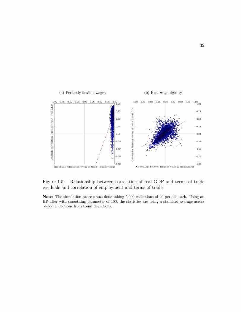
terms of trade and real GDP and labor interact. Figure 1.5 shows this relationshipwith and without the real wage rigidity. The data shows that there is a positiverelationship between these correlations from Figure 1.2(a). The model withouta real wage rigidity shows almost no relationship whatsoever as shown in Figure1.5(a). On the other hand, adding the friction in the labor market replicates whatthe data shows, as shown in Figure 1.5(b). As the correlation between terms oftrade and labor increases, the correlation between terms of trade and real GDPincreases also. Most importantly, it is able to replicate the heterogeneity in theresponses from real GDP and employment due to fluctuations in the terms oftrade.

In addition, Figure 1.6 analyzes the responses to the unemployment rate inthe model. It is expected that in the flexible wages environment, there will beno possible action in this dimension because full-employment is always achieved.Recalling from Figure 1.2(a), there exists a negative relationship between theresponses of real GDP and unemployment rates to fluctuations in the terms oftrade in the data. Figure 1.6(a) shows that it is impossible to replicate the neg-ative relationship shown in the data. On the other hand, Figure 1.6(b) is able toreplicate the heterogeneity and relationship that the responses of unemploymentand real GDP have in the data.

1.6 Conclusion

In this paper, I argue that a terms of trade deterioration can affect positivelyand negatively real GDP. I document that the business cycles correlation between

30

terms of trade and real GDP vary widely between positive and negative valuesacross 122 countries. Furthermore, this variation still persists after separatingthe countries into different income groups. I show evidence that how countriesreact towards terms of trade movements is tightly linked to their labor market.Specifically, when unemployment reacts positively to increases in the terms oftrade, real GDP will react negatively. In addition, when employment reactsnegatively to increases in the terms of trade, real GDP will also react negatively.

I construct a real business cycle model with terms of trade and productivityuncertainty and a friction in the labor market. I find that a friction in the labormarket as a real wage floor can produce a different response in macroeconomicaggregates to fluctuations in the terms of trade. In particular, when the wagerigidity is not binding, a deterioration in the terms of trade produces an increaseto real GDP and employment. On the other hand, when the wage constraintbinds, unemployment must increase to stop the fall in real wages when there isa deterioration in the terms of trade. This is, employment and real GDP fall tokeep real wages on the real wage floor level.

Finally, I due a simulation experiment of the model and analyze the resultsunder a perfectly flexible wages and under a real wage floor. I find that underno frictions in the labor market, it is not possible to replicate the heterogeneityin the responses of real GDP, employment and unemployment rates to termsof trade fluctuations. On the other hand, when there are frictions in the labormarket, the model is able to replicate the features in the data.

31

l, L

w

L0L2 L1 L3

w0

w1

w2

zFL (K0, L,M0)

zFL (K0, L,M1)

ul(c0,l)uc(c0,l)

ul(c1,l)uc(c1,l)

w

A

C

B

Figure 1.4: Representation of a negative terms of trade shock

32

(a) Perfectly flexible wages

-1.00 -0.75 -0.50 -0.25 0.00 0.25 0.50 0.75 1.00

-1.00

-0.75

-0.50

-0.25

0.00

0.25

0.50

0.75

1.00

Residuals correlation terms of trade - employment

Residuals

correlationterm

softrade-realGDP

(b) Real wage rigidity

-1.00 -0.75 -0.50 -0.25 0.00 0.25 0.50 0.75 1.00

-1.00

-0.75

-0.50

-0.25

0.00

0.25

0.50

0.75

1.00

Correlationbetweenterm

softrade&

realGDP

Correlation between terms of trade & employment

Figure 1.5: Relationship between correlation of real GDP and terms of traderesiduals and correlation of employment and terms of trade

Note: The simulation process was done taking 5,000 collections of 40 periods each. Using anHP-filter with smoothing parameter of 100, the statistics are using a standard average acrossperiod collections from trend deviations.

33

(a) Perfectly flexible wages

-1.00 -0.75 -0.50 -0.25 0.00 0.25 0.50 0.75 1.00

-1.00

-0.75

-0.50

-0.25

0.00

0.25

0.50

0.75

1.00

Correlationbetweenterm

softrade&

realGDP

Correlation between terms of trade & unemployment

(b) Real wage rigidity

-1.00 -0.75 -0.50 -0.25 0.00 0.25 0.50 0.75 1.00

-1.00

-0.75

-0.50

-0.25

0.00

0.25

0.50

0.75

1.00

Correlationbetweenterm

softrade&

realGDP

Correlation between terms of trade & unemployment

Figure 1.6: Relationship between correlation of real GDP and terms of traderesiduals and correlation of unemployment rates and terms of trade

Note: The simulation process was done taking 5,000 collections of 40 periods each. Using anHP-filter with smoothing parameter of 100, the statistics are using a standard average acrossperiod collections from trend deviations.

Chapter 2

Sovereign spread movements inemerging economies: terms oftrade matter

2.1 Introduction

This paper focuses on the high mean and volatility of interest rate spreads inemerging economies. We document that some emerging economies experience adecrease in the negative correlation between real GDP and interest rate spreadsfor the last two decades. As a matter of fact, it is observed in the data thatinterest rates oscillates regardless of a favorable domestic economic performance.Figure 2.1 shows the Mexican interest rate spread for the last twenty years andits relationship with real GDP and terms of trade. The interest rate spread inMexico displays sharp rises in 1998 and 2014, even though the economy does

34

35

not experience deep recessions during these years. Moreover, during these years,the interest rate spread in Mexico follow more closely the movements of theterms of trade series. This observation corresponds to the puzzle proposed inTomz and Wright (2007). They found that the negative correlation betweenoutput and default of a country is remarkably week. Also, they show evidenceof countries defaulting on their sovereign debts during good times while makingrepayments during bad times. This paper addresses this puzzle by arguing thatforeign conditions can explain this issue.

Figure 2.1: Spreads and Cyclical Components in Mexico

The framework presented in Eaton and Gersovitz (1981) is beneficial to ana-lyze the spread behavior because this class of model is able to derive the interestrates endogenously 1. However, it has been proven difficult to obtain three fea-

1Aguiar and Gopinath (2007) and Neumeyer and Perri (2005) assume exogenous interestrates since it is useful to explain business cycles of developing countries. High volatility andcountercyclicality of interest rates are regarded as crucial parts to explain the cyclical movementof aggregate output and prices.

36

tures of the interest rates with sovereign default models. Arellano (2008) showscountercyclical interest rate spreads by introducing convex costs of default. Thisyields defaults to be more likely to occur during recessions. Nevertheless, themean spread that the model provides is 3.58% which is relatively low comparedto the mean spread of Argentina, which is 10.25%. Also, only few fluctuations ofspread are observed with good economic conditions due to the structural featuresof the probability of default. In fact, the spread generated by the model is al-most zero when the country is hit by good endowment shocks. Mendoza and Yue(2011) achieve large volatility of spread in their baseline model by introducingendogenous default costs, but fail also to capture the high mean spread shownin the data. This is because spread and default probabilities are linked to eachother directly. Hatchondo and Martinez (2009) and Chatterjee and Eyigungor(2012) are able to improve the spread behavior in the sovereign default modelsby incorporating long-duration bonds. This helps to increase mean and standarddeviation of spread; however, those studies cannot explain why spreads can behigh during good times in the economy. The high volatility of spreads is mainlyaccomplished by the large dispersion of spreads with low endowments while thestandard deviation with high endowments is significantly small.

This paper proposes a stochastic general equilibrium model of sovereign de-fault with endogenous default risk in order to explain the interest rate behaviorin emerging economies. The key feature of this paper is that the model incorpo-rate an exogenous foreign shock called terms of trade. In the model, a negativeterms of trade shock act in two ways. First, the country spends more in foreignproducts for consumption. Second, the terms of trade have direct impacts on thelevel of foreign currency debts that sovereigns owe to foreign lender. This modelworks with the assumption that sovereigns issue their bonds in foreign prices.

37

As shown in Eichengreen and Hausmann (1999) and Jeanne (2003), emergingeconomies tend to issue debt in foreign currency because their local currencypresent high fluctuations and lack of credibility 2 Since debt is issued in for-eign currency, the countries are vulnerable to changes in world prices. In otherwords, when the adverse terms of trade shocks hit the economy, the sovereignimmediately encounters an unexpected enlarged debt burden. Consequently, theprobability of default is not only affected by countries GDP shocks but also theterms of trade shocks. This provides an explanation of why terms of trade shockscan lead to higher and more volatile spread movements, regardless of the GDPperformance.

As mentioned above developing countries experience high volatility of termsof trade and output. More specifically, terms of trade shocks are more volatilethan GDP shocks in emerging economies. This implies that the terms of tradeshocks are an important factor to consider when studying them. Moreover, asshown in Kose (2002) an important source for the repayment of foreign debtis export revenue and this is largely affected by the terms of trade. Terms oftrade are often studied in the sovereign default models. Na, Schmitt-Grohé,Uribe and Yue (2014), Gu (2015), and Asonuma (2016) endogenously induce thedeterioration of the terms of trade and real exchange rate. This paper makedistinctions from those papers by assuming terms of trade shocks as exogenous.Popov and Popov, Wiczer et al. (2014) assume an exogenous path of terms oftrade but he examines the role of terms of trade penalties and focuses on changesin trade volumes. In contrast, we focus in analyzing the changes in debt burdencontingent to terms of trade. Cuadra and Sapriza (2006) study also an exogenous

2Du and Schreger (2015) show that foreign currency debt composition has decreased since2004. Nevertheless, they still have a significant level of foreign currency debt.

38

terms of trade shock when the production side buy intermediate imported goods.In their model, the terms of trade shocks are used as if they are productivityshocks so the terms of trade shocks generate real GDP movement. However, thismechanism violates the result in Kehoe and Ruhl (2008) that proves that termsof trade do not have first order effects in real GDP3. Moreover, they do not havethe convex default costs so the frequency of default generated by the model isunusually small. In this paper we involve both endowment shocks and the termsof trade shocks, while also considering a convex default cost.

The rest of the paper is organized as follows. Section 2 empirical evidence,Section 3 the model, Section 4 quantitative analysis, Section 5 conclusion.

2.2 Empirical evidence

2.2.1 Currency composition of sovereign external debt

In this section, we construct the ratio of foreign currency sovereign externaldebt to total debt in developing countries. This helps to develop the idea thatthe terms of trade shocks are of importance to the fluctuations of the economy inemerging economies via foreign currency sovereign debt owed to foreign investors.The definition of external debt is adopted from Du and Schreger (2015). Wedeviate from their methodology because we are only interested in studying thegovernment debt4. Hence, we use the definition of sovereign external debt as any

3They also show that the terms of trade do not act as a productivity shock in standardmodels while they do affect real income and consumption in a country.

4Their definition of external debt includes both public and private debt in order to analyzehow default decisions are affected by debt denomination in public and private sectors. However,this paper considers only public debt. Thus, we define sovereign external debt instead of external

39

debt issued by the government in developing countries and owed to nonresidents,regardless of the market of issuance.

Debt is categorized by three dimensions: issue sector, issue currency, and is-sue market. Issuance sector is divided into the government and the corporatesector. The debt issued by the central or local governments is counted as gov-ernment debt while all debt issued by the private sector is regarded as corporatedebt. The classification of issue currency is determined by which currency debt isdenominated when issued. Local currency (LC) debt refers to debt that is issuedin the currency of issuance country while foreign currency (FC) debt is denomi-nated in another country’s currency. Lastly, issuance market is broken down intotwo markets. When debt is issued under the domestic law inside a country, it iscalled domestic debt; on the other hand, international debt follows foreign lawand issued in international markets. Among these categories, this paper mainlyaddress the combined category of government as issuer sector, foreign currencyas issue currency, and both markets as issue market in order to study sovereignexternal debt.

Bank for International Settlements (BIS) provides amount of outstanding debtdata by each classification. However, debt data by debt holder - nonresidents orresidents -, which is the main part of definition of external debt, are not available.Hence, we follow Du and Schreger (2015) to construct the currency composition ofsovereign external debt. They make two assumptions for debt holding of nonres-idents. First, nonresidents hold all debts in international market, which impliesthat all international debts are regarded as external debt. Second, nonresidentsdo not hold any FC debt in domestic market5. Based on these two assumptions,

debt.5They document that the amount of outstanding foreign currency debt in domestic market

40

the FC sovereign external debt is constructed as follows: amount of outstandingFC debt issued by the government in international market.

Table 2.1 provides the share of FC sovereign external debt in total sovereigndebt. The total sovereign debt is defined as all debts issued by the government soit consists of both domestic debt and external debt. 6 The analysis of this paperis proceed based on sovereign external debt, and it is expected that countries withhigher share of external debt denominated in FC are more likely to be exposedby terms of trade shocks. In Table 2.1, although the substantial heterogeneity forthe ratio of FC external debt to total debt is observed, it is sensible that countriesare considerably under the influence of it. Moreover, there are some countriesthat heavily rely on FC debt owed to foreign creditors such as Peru, Argentina,Lebanon, and Lithuania. In particular, the countries that experienced sovereigndefault events have a tendency to have higher percentage of FC external debt.Argentina had carried on more than 75% of external debt in FC until the defaultperiods and reduced it to approximately 50% in the first half of the 2000’s. Perualso has been maintained high share of FC external debt on average. In case ofRussia, almost half of the total debt is FC debt owed to nonresidents in 2004which is significantly large enough to be affected by exchange rate movements.

One of the results from Du and Schreger (2015) is that sovereigns have beenusing more LC when issuing external debt in government sector so there is atendency of the decrease in the proportion of FC external debt in total externaldebt7. Nevertheless, analyzing FC external debt is worthy. Since they compare

is notably small so the second assumption is sensible.6The definition of domestic debt in this context is any debt owed to residents within the

country.7They analyze FC external debt

Total external debt while this paper analyze FC external debtExternal debt+Internal debt .

Thus the share of foreign currency external debt in this paper is affect by the amount of debt

41

Table 2.1: Foreign Currency Debt Composition

Average 2004 2015Argentina∗ 79.6 74.9 43.4

Brazil 7.3 4.9 4.4Chile 12.9 20.8 16.3

Colombia 22.8 22.8 25.5Croatia 45.7 59.3 46.1Hungary 22.7 19.8 27.0Indonesia 13.9 3.2 30.8Lebanon 35.2 51.5 44.8Lithuania 83.8 73.2 79.5Malaysia 3.9 9.0 3.3Mexico 16.2 27.3 15.1Peru∗ 65.1 84.2 38.7

Philippines 24.9 33.9 23.4Russia∗ 31.2 48.5 38.1

South Africa 7.2 10.6 9.7Turkey 19.0 16.5 29.6

Notes: * indicates countries that experienced default events. 2005 data is used for Mexico andMalaysia for the 2004 column and 2007 data and 2008 data are used for South Africa and

chile for the 2004 column respectively. They are first year of data availability.

42

the FC external debt with total external debt, the expansion or contraction of theamount of total external debt is not taken into consideration in their constructionof currency composition. In other words, the importance of FC external debtcould be underestimated if the countries issue more external debt than domesticdebt. However, the measure of currency composition used in this paper reflectsthis issue since the definition of total sovereign debt include both domestic debtand external debt. If the amount of domestic debt gets smaller, then the shareof FC external debt in total sovereign debt increases which means external debtin FC becomes a more essential part of the debt in the countries. Actually, allcountries except Hungary and Russia in Table 2.1 display continuous increases inthe amount of external debt denominated in FC.8 Furthermore, it is not explicitlyshown that the share of FC external debt has been decreasing in Figure 2.2 withour data construction. Indonesia, Hungary, Turkey, and Lithuania, for instance,have kept expanding the share of external debt in FC. The LC debt in domesticmarket rapidly rose in Croatia around 2004 so the share sharply decreased atthat time but it started to issue more FC debt in international market in 2009so the share has been following the growing trend since the time. In addition,other countries hold more or less a constant share of FC external debt. Thoseempirical evidence illustrates that external debt in FC are still a crucial part ofdebt in developing countries.

owe to residents in a country.8Hungary and Russia has been reducing the amount of foreign currency external debt since

2014.

43

Figure 2.2: Foreign Debt Profile for Emerging Economies

2.3 Terms of trade, GDP and spread across coun-tries

The data presented in Table 2.2 and 2.3 are statistics for the terms of trade,GDP, and spread across 24 developing countries. In this paper, the terms of trade(TOT) are defined as the price of imports relative to the price of exports.

TOT = PMPX

44

In order to construct the terms of trade, quarterly merchandise customs importsand exports data 1991Q1 to 2015Q4 are obtained from World Bank Global Eco-nomic Monitor (GEM). 9 By using current and constant value of import andexport each deflator is calculated. Afterwards the import and the export defla-tors are used for the price of imports and the price of exports respectively. Hence,the terms of trade are constructed by import deflator over export deflator. Thequarterly GDP is also provided from GEM and the time period is the same asthe one in imports and exports data. The interest rate spread data are takenfrom J.P. Morgan’s EMBI + database.10 The terms of trade and output are logand HP detrended.

Table 2.2 provides standard deviation of the terms of trade, GPD, and spread.It also provides the mean of spread in each country since this paper focuses on thebehavior of spread. Although there is a cross-country heterogeneity, in almost allsample countries, the standard deviations of TOT is bigger than those of GDP. Inother words, TOT is more fluctuate than GDP in most of countries. This fact iscrucial for the analysis of the paper since this indicates that more fluctuations ofthe economy can be driven by the terms of trade shocks with high volatility. Also,defaulted countries, such as Argentina, Ecuador, and Russia, show much highermean and volatile movement of spread. In particular, the volatility of TOT inEcuador is approximately 14 times bigger than its GDP. Hence, it can be seenthat Ecuador has been affected by volatile terms of trade shocks. However, it is

9World Development Indicators (WDI) provides imports and exports data across countries,but this is annual data. Thus, we interpolate annual data to transform to quarterly data andcompare it with the quarterly merchandise customs imports and exports and we found thatthose two series are coincided through the sample period.

10The spread data are not a balanced data across countries, so we used series of spreadavailable up to 2015Q4.

45

unclear that the terms of trade shocks is a main factor for movement of spreadbased on magnitude of standard deviation, but correlation with spread will helpto improve this issue.

Table 2.3 shows different combinations of correlations among TOT, GDP andspread in the sample countries. First, the negative correlations between GDP andspread are achieved and also the positive correlations between TOT and spreadare presented in most countries. This implies that the deterioration of the termsof trade coincide with the increase in spread in general. Moreover, even thoughit is hard to find a certain pattern between ρ(TOT,spread) and ρ(TOT,spread),there are nine countries having higher correlation of spread with TOT than withGDP. This can be direct evidence for the impacts of TOT on movement of interestrate spread. For example, Mexico have significantly high correlation of spreadwith TOT while there is almost no correlation with GDP: hence, it is reasonableto conclude that the the fluctuation of Mexican spread is mainly affected by theterms of trade shocks. This interpretation can be generalize to any countriesshowing higher correlation between spread and TOT.

2.4 Model

In this section, we propose a model of that incorporates two sources of uncer-tainty in a country, a domestic and a foreign. We work with a framework thatextends the sovereign default models introduced in Eaton and Gersovitz (1981)and Arellano (2008). We use this last one to incorporate a source of externaluncertainty called terms of trade.

Consider a small open economy where there are two types of shocks, a domes-tic and a foreign. On one hand, the domestic shock is going to be represented by

46

Table 2.2: Descriptive Statistics in Emerging Economies

σ(TOT) σ(GDP) σ(spread) µ(spread)Argentina 0.045 0.040 18.24 15.99Brazil 0.041 0.015 3.92 5.66Chile 0.090 0.018 0.59 1.46China 0.036 0.010 0.55 1.18

Colombia 0.073 0.013 2.07 3.56Dominican Rep 0.022 0.023 3.30 5.39

Ecuador 0.295 0.020 8.38 12.33Egypt 0.034 0.015 1.74 2.55

Hungary 0.016 0.015 1.58 1.80Indonesia 0.068 0.033 1.44 2.89Kazakhstan 0.264 0.024 2.74 4.28

Korea 0.035 0.023 1.04 1.31Malaysia 0.027 0.018 1.25 1.78Mexico 0.040 0.023 1.51 2.75Morocco 0.016 0.013 2.43 2.30Peru 0.073 0.018 1.96 3.51

Philippines 0.046 0.013 1.52 3.46Poland 0.096 0.014 0.90 1.71Russia 0.098 0.029 11.26 7.28

South Africa 0.032 0.012 1.19 2.26Sri Lanka 0.024 0.009 4.33 6.01Tunisia 0.014 0.011 0.92 1.84Turkey 0.030 0.036 2.20 4.02Ukraine 0.023 0.043 6.23 7.46

47

Table 2.3: Correlations in Emerging Economies

ρ(TOT,spread) ρ(GDP,spread) ρ(TOT,GDP)Argentina -0.026 -0.647 -0.066Brazil 0.205 -0.198 -0.553Chile 0.528 -0.335 -0.478China -0.080 -0.007 0.257

Colombia 0.267 -0.197 -0.485Dominican Rep 0.020 -0.641 -0.006

Ecuador 0.517 -0.445 -0.687Egypt 0.082 -0.189 0.084

Hungary 0.141 -0.290 0.222Indonesia 0.574 -0.284 -0.507Kazakhstan -0.440 -0.607 0.541

Korea -0.209 -0.633 0.524Malaysia 0.061 -0.485 0.116Mexico 0.443 0.005 -0.466Morocco -0.126 0.135 -0.099Peru 0.332 -0.156 -0.263

Philippines 0.029 -0.326 0.262Poland 0.007 0.159 0.137Russia 0.241 -0.487 -0.681

South Africa 0.223 -0.250 -0.021Sri Lanka 0.433 -0.430 0.229Tunisia 0.556 -0.162 0.017Turkey 0.169 -0.449 0.079Ukraine -0.194 -0.423 -0.157

48

real GDP movements. On the other, the foreign shock is going to be representedby terms of trade movements. Let yt and pt represent output and terms of tradein period t, respectively. As discussed previously, it is standard to assume termsof trade as an exogenous variable for small open economies. We consider this inorder to construct the following stochastic system

ln yt+1

ln pt+1

= A

ln ytln pt

+εyt+1

εpt+1

, (2.1)

where the roots of the second order polynomial det (I2 − Ax) = 0 lie outside thecomplex unit circle and the errors vector is a binormal distribution with mean 0and variance-covariance matrix Σ. With this formulation we are able to tailor acorrelation between contemporanous real GDP and terms of trade.11

There are two types of tradable goods in this economy, a domestic and aforeign. In every period, a representative household purchases these two typesof goods and transfom them into a final consumption good using the followingArmington aggregator technology,

C =(λc−ηd + (1− λ)c−ηf

)− 1η ,

where C represents the final aggregated good consumption, cd the domestic goodconsumption, cf the foreign good consumption, λ ∈ [0, 1] a parameter that cap-tures home bias, and η ∈ [−1,∞) a parameter that controls the elasticity of

11As shown in Kehoe and Ruhl (2008), it is a common mistake to misrepresent what realGDP is in a model. Moreover, standard models with a production side that buy imported goodsat the price of terms of trade capture a spurious correlation between real GDP and terms oftrade. If real GDP is measured correctly in them, the correlation between real GDP and termsof trade should be close to zero.

49

substitution between domestic and foreign goods. The representative householdis able to purchase these goods taking the output available in the period andan amount of taxes that the government issues in a lump-sum fashion as given.The representative household is a risk averse agent that obtains utility from thestream of final consumption goods obtained in every period as

E0

[ ∞∑t=0

βtu (Ct)],

where β ∈ (0, 1) is a parameter that captures a discount factor across periodsand u(·) is an increasing and strictly concave function.

In this economy there is also a benevolent government whose objective is tomaximize the utility of the representative household. In order to achieve this, ithas two main decisions to take. The first decision is either to honor or default inits sovereign bonds obligations. If the government takes the decision of honoringthem, it has access to international financial markets where it can buy or sellone period maturity sovereign bonds. Then, the second decision is how much ofthese bonds to purchase given a price schedule contingent to the amount of thesenew bonds and the shocks the economy experiences. Let B, B′, and q(B′, y, p)represent the amount of sovereign bonds due, the amount of new sovereign bondspurchases, and the price of these at any given period.

We introduce the assumption that the international financial markets aremanaged only in foreign goods. This is, the sovereign bonds returns and purchaseshave to be done in foreign terms. Because of this, the value of sovereign bondsin each period will be subject to the terms of trade shock.

We model two types of penalties for defaulting in sovereign debt, exclusion offinancial markets and output losses. With these penalties we want to capture the

50

fact that countries that default in their debt experience a temporary exclusion tointernational borrowing and periods of poor output performance. We assume thatif a government defaults in their debt, this will be erase entirely and it will entera financial autarkic environment. In addition, the country will experience anoutput cost that limit its endowment. The economy will remain in this financialautarky for a stochastic number of periods and will re-enter the financial marketswith an exogenous probability.

Let x represent exports, the resources exiting the economy. The balance tradecondition for the repayment state can be expressed as

x− pcf = pq(B′, y, p)B′ − pB.

The left-hand side is the current account while the right-hand side is the negativeof the capital account of the economy. This is, any surplus(deficit) that the capitalaccount experiences due to the government’s sovereign debt position will implya deficit(surplus) of the current account. The balance trade condition for thedefault state can be expressed as

x− pcf = 0.

Considering the exclusion of financial markets penalty of default, the balancetrade condition will imply that the current account cannot experience any kindof suplus or deficit.

The resource constraint of the government will show how the domestic goodendowment can be consumed in every period. On one hand, if the government

51

chooses to repay its debt, the resource constraint will be

cd + x = y.

On the other hand, if the government chooses to default,

cd + x = h(y),

where h(·) is an increasing function such that h(y) ≤ y12.There is a representative foreign lender who is able to borrow and lend risk-

free bonds at a constant international interest rate r∗ > 0. We assume it hasperfect information about the small open economy. This is, it can observe thelevel of output and terms of trade that the small open economy experiencesevery period. The foreign lender is risk neutral13 and maximizes expected profitsover risky sovereign bonds from the small open economy. We assume that theforeign lender maximizes profit only in foreign goods terms. Let δ represent theprobability of the government to default in its sovereign debt position. Takingas given the default probability and the bond price, the foreign creditor choosesB′ to maximizes

MaxB′

{qB′ −

(1− δ1 + r∗

)B′}.

By the risk neutral nature of the foreign lender, the bond price schedule solu-12Realise that the output cost is defined as y − h(y) and is non-negative by definition.13Cole and Kehoe (1996) explains that the risk neutrality of the foreign lenders reflect the

fact that the size of an individual sovereign transaction is relatively small compared to the totalinternational credit market.

52

tion in equilibrium must satisfy the first order condition of the previous problem.The bond price schedule will be a result of the following break-even condition,

q = 1− δ1 + r∗

. (2.2)

Realising that δ ∈ [0, 1], we can infer that q ∈[0, 1

1+r∗]. Defining the sovereign

interest rate as r ≡ 1q− 1, we obtain that r = [r∗,∞). Finally, we define the

sovereign bond spread as S ≡ r − r∗.The timing of the government problem is the following. In the beginning

of the period the government realises the amount of sovereign bonds due B,the domestic goods endowent shock y, and the terms of trade shock p. Thegovernment asses the optimal relationship between domestic and foreign goodsusing p and the preferences of the representative household. Then the governmentdecides whether to honor or default in its debt obigations. If it decides to honor itsdebt, the government updates its sovereign bond holdeings B′ taking as given thesovereign bond price schedule q(B′, y, p) and constrained to its resource constraintand the balance trade condition. The foreign lender takes the bond price q asgiven and supplies B′ matching B′. Purchases of foreign and domestic take place.Finally, the representative household consumes the final good by aggregating thedomestic and foreign goods.

2.4.1 Recursive Equilibrium

There are three variables that define the state of the government in everyperiod: the sovereign bonds due, the output shock, and the terms of trade shock.Define V (B, y, p) as the value function of the government at the beginning of

53

every period. Let us model the first decision of the government as

V (B, y, p) = Max{V R(B, y, p), V D(y, p)

}, (2.3)

where V R(B, y, p) and V D(y, p) represent the value of the government if it repaysand defaults in its debt obligations, respectively. Here, the government chooseswhich environment will yield the highest welfare for the representative householdcaptured by V R(B, y, p) and V D(y, p).

When the government chooses to repay, it chooses the amount of sovereignbonds to sell or purchase as well as the household allocations that will maximizeits welfare subject to the resource constraint, the balance trade condition, theaggregation technology, and a no-Ponzi condition. In order to do this, it takesthe price schedule for the bonds as given and a lower boundary for the sovereignbonds issuance B > 0. Thus,

V R(B, y, p) = Maxx,cd,cf ,C,B′

{u(C) + βE(y′,p′) [V (B′, y′, p′)|(y, p)]

}(2.4)

s.t. cd + x = y (Resource Constraint)

x− pcf = pq(B′, y, p)B′ − pB(Balance Trade Condition)

C =(λc−ηd + (1− λ)c−ηf

)− 1η (Aggregation Technology)

B′ ≥ −B. (No-Ponzi Condition)

When the government chooses to default, it chooses the household allocationsthat will maximize its welfare subject to the resource constraint, the balancetrade condition, and the aggregation technology. In order to do this, it takes

54

the default penaltiy and the probability of returning to the financial marketsφ ∈ [0, 1] as given. Recall that the default penalties are the output costs and thezero current account restriction due to the financial market exclusion. Thus,

V D(y, p) = Maxx,cd,cf ,C

{u(C) + βE(y′,p′)

[φV (0, y′, p′) + (1− φ)V D(y′, p′)|(y, p)

]}(2.5)

s.t. cd + x = h(y) (Resource Constraint)

x− pcf = 0 (Balance Trade Condition)

C =(λc−ηd + (1− λ)c−ηf

)− 1η . (Aggregation Technology)

In order to define what is the probability of default for a government, itis useful to characterize the set of output and terms of trade states in whicha government finds optimal to default contingent to a level of sovereign bondholdings. Specifically, define the default set as the

D(B) ={

(y, p) ∈ R2++ : V D(y, p) > V R(B, y, p)

}. (2.6)

This set expresses that if the government sells B′ and the shocks of next periodare (y′, p′) ∈ D(B′), then the government will find it optimal to default on B′

next period. Because of this, we can define the probability for a governmentto default on B′ by measuring how likely is to end up in the states that live inD(B′). Given the stochastic process that govern the movements of output andterms of trade shocks, call f(·) the probability density function between shock

55

states. Thus, the probability of default can be expressed as

δ(B′, y, p) =∫

(y′,p′)∈D(B′)f ((y′, p′)|(y, p)) d(y′, p′). (2.7)

Consider the case where the government chooses a level of sovereign bonds B′

such that there are no possible states in the next period in which it will default onthem, D(B′) = ∅. Then, with that amount of sovereign bonds the probability ofdefault will be zero, δ(B′, y, p) = 0. Also, consider the case when the governmentchooses a level of sovereign bonds B′ such that default is for sure regardlessof the shock realisations in the next period, D(B′) = R2

++. Then, with thatamount of sovereign bonds the probability of default will be one, δ(B′, y, p) = 1.Finally, realise that if the output and terms of trade shocks have no persistencywhatsoever, then the probability of default will only be contingent in the sovereignbond issues or purchases.

Now, the bond price schedule must satisfy the break-even condition (2.2) fromthe representative foreign lender problem. Considering the probability of default,the representative foreign lender must be consistent to (2.7). Thus, the bondprice schedule will be

q(B′, y, p) = 1− δ(B′, y, p)1 + r∗

. (2.8)

Realise that this break-even condition will yield zero profit in expectation tothe representative foreign lender regardless of the quantity of sovereign bondsit purchases or sells B′. Therefore, it will be willing to cover any amount ofsovereign bonds the government finds optimal to choose during the repaymentstate. In other words, the sovereign bond market always clear in equilibrium

56

B′ = B′.

Definition 2 (Recursive Equilibrium) The recursive equilibrium of this smallopen economy will be a set of government value functions V (B, y, p), V R(B, y, p),V D(y, p) and a sovereign bonds policy rule B′(B, y, p), a set of household con-sumption policy rules cd(B, y, p), cf (B, y, p), and C(B, y, p), an exports policyrule x(B, y, p), a default set D(B, y, p), a default probability schedule δ(B, y, p),and bond price schedule q(B, y, p) such that the following conditions are satisfied:

I Benevolent Government (Initial)The default set D(B, y, p) is consistent with the set of government valuefunctions V (B, y, p), V R(B, y, p), and V D(y, p) and solves (2.3).

I Benevolent Government (Repayment)If (y, p) /∈ D(B) and taking as given the bond price schedule q(B, y, p), thegovernment chooses the sovereign bonds policy rule B′(B, y, p), the set ofhousehold consumption policy rules cd(B, y, p), cf (B, y, p), and C(B, y, p),and the exports policy rule x(B, y, p) in order to solve (2.4) and its solutionis consistent with V R(B, y, p).

I Benevolent Government (Default)If (y, p) ∈ D(B), the government chooses the set of household consumptionpolicy rules cd(B, y, p), cf (B, y, p), and C(B, y, p), and the exports policyrule x(B, y, p) in order to solve (2.5) and its solution is consistent withV D(y, p).

I Default probabilityThe default probability schedule δ(B, y, p) is consistent with the default setD(B, y, p) and (2.7).

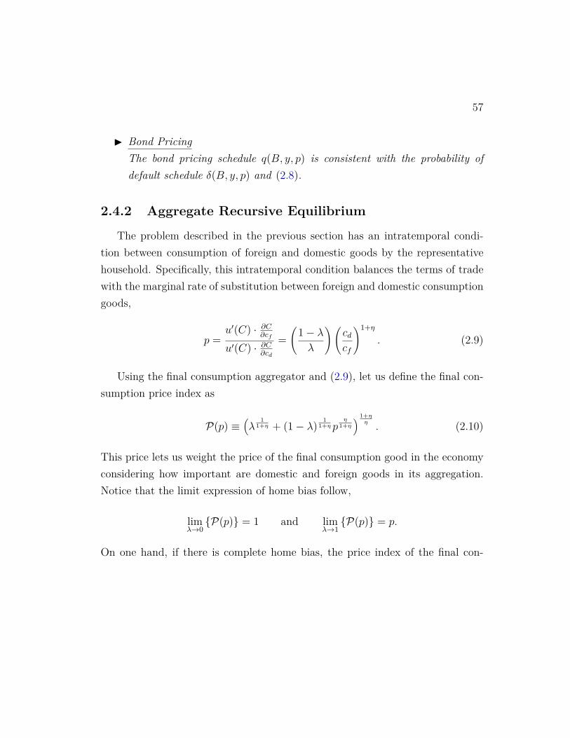
57

I Bond PricingThe bond pricing schedule q(B, y, p) is consistent with the probability ofdefault schedule δ(B, y, p) and (2.8).

2.4.2 Aggregate Recursive Equilibrium

The problem described in the previous section has an intratemporal condi-tion between consumption of foreign and domestic goods by the representativehousehold. Specifically, this intratemporal condition balances the terms of tradewith the marginal rate of substitution between foreign and domestic consumptiongoods,

p =u′(C) · ∂C

∂cf

u′(C) · ∂C∂cd

=(

1− λλ

)(cdcf

)1+η

. (2.9)

Using the final consumption aggregator and (2.9), let us define the final con-sumption price index as

P(p) ≡(λ

11+η + (1− λ)

11+η p

η1+η) 1+η

η. (2.10)

This price lets us weight the price of the final consumption good in the economyconsidering how important are domestic and foreign goods in its aggregation.Notice that the limit expression of home bias follow,

limλ→0{P(p)} = 1 and lim

λ→1{P(p)} = p.

On one hand, if there is complete home bias, the price index of the final con-

58

sumption good is not affected at all by the terms of trade. This result is intuitivebecause it tells us that the representative household does not derive any utilityfrom foreign consumption goods. On the other hand, if there is complete foreignbias, the price index of the final consumption good is the complete terms of tradeprice.

Consider an aggregate version of the government’s problem when it choosesto repay,

V R(B, y, p) = MaxC,B′

{u(C) + βE(y′,p′) [V (B′, y′, p′)|(y, p)]

}(2.11)

s.t. P(p)C + pq(B′, y, p) = y + pB (Resource Constraint)

B′ ≥ −B. (No-Ponzi Condition)

Also, consider the an aggregate version of the government’s problem when itchooses to default,

V D(y, p) = Maxcd,cf ,C

{u(C) + βE(y′,p′)

[φV (0, y′, p′) + (1− φ)V D(y′, p′)|(y, p)

]}(2.12)

s.t. P (p)C = h(y) (Resource Constraint)

Definition 3 (Aggregate Recursive Equilibrium) The aggregate recursiveequilibrium of this small open economy will be a set of government value functionsV (B, y, p), V R(B, y, p), V D(y, p) and a sovereign bonds policy rule B′(B, y, p), ahousehold final consumption policy rule C(B, y, p), a final consumption good priceindex P(p), a default set D(B, y, p), a default probability schedule δ(B, y, p), andbond price schedule q(B, y, p) such that the following conditions are satisfied:

59

I Benevolent Government (Initial)The default set D(B, y, p) is consistent with the set of government valuefunctions V (B, y, p), V R(B, y, p), and V D(y, p) and solves (2.3).

I Benevolent Government (Repayment)If (y, p) /∈ D(B) and taking as given the bond price schedule q(B, y, p) andthe final consumption good price index P(p), the government chooses thesovereign bonds policy rule B′(B, y, p) and the household final consumptionpolicy rule C(B, y, p) in order to solve (2.4) and its solution is consistentwith V R(B, y, p).

I Benevolent Government (Default)If (y, p) ∈ D(B) and taking as given the final consumption good price in-dex P(p), the government chooses household final consumption policy rulesC(B, y, p) in order to solve (2.5) and its solution is consistent with V D(y, p).

I Price IndexThe final consumption good price index follows (2.10).

I Default probabilityThe default probability schedule δ(B, y, p) is consistent with the default setD(B, y, p) and (2.7).

I Bond PricingThe bond pricing schedule q(B, y, p) is consistent with the probability ofdefault schedule δ(B, y, p) and (2.8).

Proposition 4 (Recursive Equilibrium Isomorphism) The equilibriums de-fined in Definition 2 and Definition 3 are isomorphic.

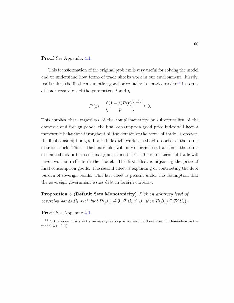
60

Proof See Appendix 4.1.

This transformation of the original problem is very useful for solving the modeland to understand how terms of trade shocks work in our environment. Firstly,realise that the final consumption good price index is non-decreasing14 in termsof trade regardless of the parameters λ and η,

P ′(p) =(

(1− λ)P (p)p

) 11+η

≥ 0.

This implies that, regardless of the complementarity or substitutaility of thedomestic and foreign goods, the final consumption good price index will keep amonotonic behaviour throughout all the domain of the terms of trade. Moreover,the final consumption good price index will work as a shock absorber of the termsof trade shock. This is, the households will only experience a fraction of the termsof trade shock in terms of final good expenditure. Therefore, terms of trade willhave two main effects in the model. The first effect is adjsuting the price offinal consumption goods. The second effect is expanding or contracting the debtburden of soverign bonds. This last effect is present under the assumption thatthe sovereign government issues debt in foreign currency.

Proposition 5 (Default Sets Monotonicity) Pick an arbitrary level ofsovereign bonds B1 such that D(B1) 6= ∅, if B2 ≤ B1 then D(B1) ⊆ D(B2).

Proof See Appendix 4.1.14Furthermore, it is strictly increasing as long as we assume there is no full home-bias in the

model λ ∈ [0, 1)

61

This result is originally taken from Eaton and Gersovitz (1981), Arellano(2008), and Chatterjee, Corbae, Nakajima and Rios-Rull (2007) and it is commonin sovereign default models. This result tells us that incentives are monotonicwith respect of sovereign bonds. Hence, it is mainly followed because the bondpricing q(B′, y, p) is independent from the sovereign bonds due in a period. Inour model, this relationship does not exist because of the assumption of riskneutrality from the representative foreign lender. Thus, given a level of outputand terms of trade, the sovereign bonds due in the period acts only as a shifterin the available amount of resources in the economy. Therefore, if for a level ofsovereign bonds a government finds optimal to default, then for a lower level ofsoverign bonds the default decision will still be optimal because the governmentwill have less resources overall.

Using Proposition 5 we can conclude that the bond pricing q(B, y, p) is non-decreasing in sovereign bonds. Let us focus in the case where the governmentborrows resources from foreign lenders. As the government increases the amountof borrowing, the actual amount of resources received will decrease because thebond pricing contracts. This resources reduction of borrowing compensates thedefault probability that the government can incur in the following period.

2.4.3 No Persistency Case

Let us study the case in which the stochastic system proposed in (2.1) has nopersistency, therefore it is i.i.d. binormal distribution with mean 0 and variance-covariance matrix Σ. In this case, the probability of default and the sovereignbond price schedule lose their contingency with respect of GDP and terms oftrade. This is because current levels of GDP and TOT do not provide any

62

information about the future realizations of them. We assume also that there areno penalty costs, h(y) = y; and default is permanent, φ = 0.

Proposition 6 (No Resources Inflows) For every sovereign bonds B such thatD(B) 6= ∅, every feasible B′ will yield no resources inflows, q(B′)B′ −B ≥ 0.

Proof See Appendix 4.1.

Default episodes happen when governments are unable to roll-over their debt.This idea is captured with Proposition 6. If the government is in a state wherehe chooses to default, all the feasible issuances of sovereign bonds must have notbeen enough to cover the sovereign bonds due in the period. Specifically, therewas no feasible issuances of sovereign bonds that could have given a positive fluxof resources from outside, B − q(B′)B′ ≯ 0.

Proposition 7 (GDP Default Incentives) Pick an arbitrary level of terms oftrade p and sovereign bonds B such that D(B) 6= ∅, if y2 ≤ y1 and (y1, p) ∈ D(B)then (y2, p) ∈ D(B).

Proof See Appendix 4.1.

Default episodes also happen when economies experience recessions, periodswhere GDP levels are below the trend. Proposition 7 is able to capture thisidea. This shows that there if a government finds optimal to default on a level ofsovereign bonds for a given recession, any deeper recession would make it defaultas well. This result is driven mainly because the country will be poorer and thereare not contracts available that provide an influx of resources from abroad.

63

Proposition 8 (Terms of Trade Default Incentives) Pick an arbitrary levelof GDP y and sovereign bonds B such that D(B) 6= ∅, if p2 ≥ p1 and (y, p1) ∈D(B) then (y, p2) ∈ D(B).

Proof See Appendix 4.1.

We have a similar result for the case of terms of trade rising higher than thetrend. Proposition 8 is able to capture this idea. This shows that there if agovernment finds optimal to default on a level of sovereign bonds for a level ofterms of trade, any higher level of terms of trade would make it default as well.This result is driven mainly because the country will experience more expensivegoods from the exterior and the resources that flow outside the country will growbecause of the foreign good coversion.

2.5 Quantitative analysis

In this section, we study Mexico and its business cycles statistics. Also, we de-scribe the calibration process of the model fitting the parameters to the Mexicaneconomy. We solve the aggregate recursive equilibrium described in Definition3 applying a value function iteration process using a grid search method. Thecomplete algorithm can be found in Appendix 4.2.

2.5.1 Data

Let us study the Mexican business cycle behavior as an emerging economy.Using OECD Statistics, we obtain quarterly data seasonally adjusted at quarterlylevels, and at current and constant prices from 1993Q1 to 2016Q2 for the series

64

of gross domestic product, private final consumption expenditure, exports of goodsand services, and imports of goods and services. Also, using Global FinancialDatabase, we obtain quarterly data from 1997Q4 to 2016Q3 for the series ofEmerging Markets Bond Index (EMBI+). The series of EMBI+ is provided byJ.P. Morgan and portrays the long-term spread between yields from sovereignbond and the U.S. Treasuries. We construct the terms of trade series as the ratioof imports price delfator and exports price deflator following Kehoe and Ruhl(2008) methodology15. We apply the HP-filter with a smoothing parameter of1600 to the real consumption, real output and terms of trade log-series in orderto obtain the cyclical components of them. In addition, we compute the ratio ofthe difference between exports and imports, over GDP to construct the series oftrade balance.

Table 2.4: Business Cycles Statistics for Mexico

Variable µ σ ρ(·,Spread) ρ(·,GDP) ρ(·,TOT)Spread 2.71% 1.47% - 0.0352 0.2178GDP - 2.22% 0.0352 - -0.4480

Terms of Trade - 2.56% 0.2178 -0.4480 -Consumption - 2.65% -0.0367 0.9518 -0.4673Trade Balance -0.84% 1.62% 0.3335 -0.4819 0.1501

Table 2.4 shows the business cycles statistics for the Mexican economy. Thetable shows regular characteristics of emerging economies shown in Neumeyer and

15There are other ways to compute terms of trade. For example, Mendoza (1995) uses theratio of exports and imports volumes. We choose not to use this methodology for convenience.Establishing terms of trade as the ratio of imports and exports deflator matches closely themovements of real exchange rates.

65

Perri (2005). The volatility of consumption is higher compared to the volatility ofGDP. Another important characteristic is that trade balance is countercyclical.Nevertheless, we are not able to find that interest rates (captured by the sovereignspread series) are countercyclical after 1997Q416.

Terms of trade also play an important feature. As documented in Mendoza(1995), Kose (2002), and Broda (2004), there is a strong negative relationshipbetween terms of trade and real GDP in emerging countries. Also, the volatilityof terms of trade is higher compared to the volatility of GDP. An importantfeature we are able to provide is that the correlation between terms of trade andthe spreads is significantly higher than the correlation between GDP and spreads.This seems to suggest that the movements the Mexican experienced after 1997may be better explained by movements in terms of trade rather than movementsin real GDP.

2.5.2 Calibration

We use the real GDP and terms of trade HP-filter log-series in order to esti-mate (2.1). We assume that the errors vector components are independent fromeach other17 and distributed as εyt+1 ∼ N(0, σ2

y) and εyt+1 ∼ N(0, σ2

y). We estimate16We analyzed this issue further. We use the database provided by Neumeyer and Perri

(2005) and construct an implied EMBI+ series from 1994Q1 to 1997Q3. In the databasethe authors provide the interest rate of several emerging economies from 1994Q1 to 2002Q2.We take the series of Mexican interest rates and substract the yield of US 10-year Treasuryconstant maturity. We find that the constucted EMBI+ series resembles closely the originalEMBI+ series in the quarters they overlap with the exception of the period 2001Q2-2002Q2.Filling the missing quarters for the spread series we are able to find that the interest rates(captured by the sovereign spread series) is countercyclical, with a correlation of -0.4275.

17We make this assumption for simplicity. Nevertheless, we are expecting in relaxing this.The error of the real GDP regression surely is correlated with contemporanous terms of trade.

66

the matrix A using standard OLS regressions18,

A = 0.8399 −0.0291−0.1466 0.5367

.Once estimated the matrix A, we recover the observed errors and estimate thestandard deviations of the errors. The standard deviations of the GDP andterms of trade errors are σy = 0.0105 and σp = 0.0203, respectively. Finally,we discretize the 2-dimensional VAR(1) process into a 289 Markov chain (17GDP and 17 terms of trade shock levels) using a quadrature method algorithmfollowing Tauchen and Hussey (1991) with a 3 standard deviations mean centeredbandwidth.

We use a standard CRRA utility function to convey the representative house-hold preferences,

u(C) = C1−σ

1− σ ,

where σ represents the constant relative risk aversion parameter. We settle thisrisk aversion parameter to the value of 2. This is a common value in the inter-national real business cycles literature.

During default episodes we impose GDP penalty via the increasing functionh(·). An important issue to address when modeling this is its sensitivity con-tingent to the state of the economy. We use Arellano (2008) convex GDP cost

In this way, the assumption of the errors being independent should be worked upon.18We make this assumption to capture a higher correlation between contemporanous real

GDP and terms of trade. Terms of trade can be considered as exogenous for small openeconomies as motivated in Broda (2004). Therefore, previous real GDP affecting contempora-neous terms of trade should be restricted.

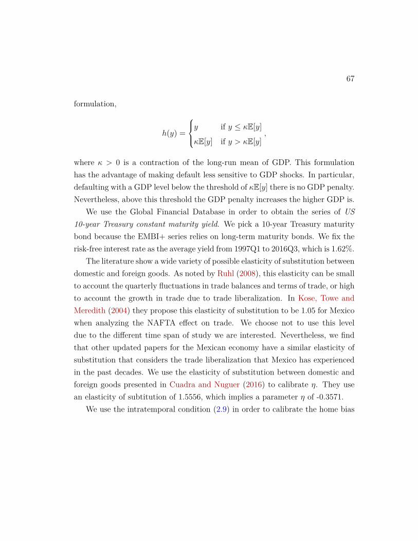
67

formulation,

h(y) =

y if y ≤ κE[y]

κE[y] if y > κE[y],

where κ > 0 is a contraction of the long-run mean of GDP. This formulationhas the advantage of making default less sensitive to GDP shocks. In particular,defaulting with a GDP level below the threshold of κE[y] there is no GDP penalty.Nevertheless, above this threshold the GDP penalty increases the higher GDP is.

We use the Global Financial Database in order to obtain the series of US10-year Treasury constant maturity yield. We pick a 10-year Treasury maturitybond because the EMBI+ series relies on long-term maturity bonds. We fix therisk-free interest rate as the average yield from 1997Q1 to 2016Q3, which is 1.62%.

The literature show a wide variety of possible elasticity of substitution betweendomestic and foreign goods. As noted by Ruhl (2008), this elasticity can be smallto account the quarterly fluctuations in trade balances and terms of trade, or highto account the growth in trade due to trade liberalization. In Kose, Towe andMeredith (2004) they propose this elasticity of substitution to be 1.05 for Mexicowhen analyzing the NAFTA effect on trade. We choose not to use this leveldue to the different time span of study we are interested. Nevertheless, we findthat other updated papers for the Mexican economy have a similar elasticity ofsubstitution that considers the trade liberalization that Mexico has experiencedin the past decades. We use the elasticity of substitution between domestic andforeign goods presented in Cuadra and Nuguer (2016) to calibrate η. They usean elasticity of subtitution of 1.5556, which implies a parameter η of -0.3571.

We use the intratemporal condition (2.9) in order to calibrate the home bias

68

parameter. Realise that the intratemporal condition can be rewritten as(cfC

)1+η= (1− λ)P(p;λ, η)

p(2.13)

In order to construct the series of consumption of foreign goods, we obtain fromthe Mexican central bank the annual share of imported consumption goods fromtotal imports from 1997 to 2015. We find that the average share is of 13.18%during this period19. Using total imports of goods and services, private finalconsumption expenditure, and terms of trade quarterly series, the parameter valueof η = −0.3571, the fixed share of imported consumption goods, and the finalconsumption good price index (2.10) formula; we find a series of the home biasλt that solves in every quarter the intratemporal condition (2.13). We find thatthe average home bias is of 0.8748 from 1997Q4 to 2016Q2.

We calibrate the default GDP penalty and the discount factor in order tomatch two moments of the Mexican economy. Mexico has defaulted in its sovereigndebt twice (1928 and 1982) in the last hundred years20. This gives a rough es-timate of a 2% default probability. We then focus the targets to be this defaultprobability and the standard deviation of trade balance over GDP ratio shownin Table 2.4. Finally, we keep the probability of re-entry to financial marketsproposed by Arellano (2008)21. Table 2.5 presents the parameters specification

19We also find that from 2007 to 2015 this share almost doubled from 8.5% to 14.24%. Wealso find that most of this increase happened in the first six years of the sample. For this reason,we consider this share as a constant for the calibration process.

20As noted in Reinhart and Rogoff (2009), the default years were when two important inter-national crises happened, the Great Depression and the Emerging Markets Crises. During theTequila Crisis in 1994, Mexico was close to default with its international lenders. Thanks tothe internatinal help from the USA, Mexico was able to have dodge this.

21In Gelos, Sahay and Sandleris (2011), it is shown that the average waiting period for re-

69

from the calibration and estimation strategy.

Table 2.5: Parameters Specification

Parameter Value Source

A

[0.8399 −0.0291−0.1466 0.5367

]OLS estimators

σy 0.0105 Observed errorsσp 0.0203 Observed errorsσ 2.00 IRBC Literaturer∗ 1.62% US 10-year Treasuryη -0.3571 Cuadra and Nuguer (2016)λ 0.8748 Intratemporal Conditionβ 0.9530 Default probabilityκ 0.9690 Trade balance volatilityφ 0.2820 Arellano (2008)

entry after a default has decreased significantly. They show that this average fell from 5 yearsin the 1980’s to 1.6 years in the 1990’s. Nevertheless, in Alessandro et al. (2011), they concludethat this comparison between decades is not fair. In particular, that the decrease in averagewaiting period for re-entry has not decreased throughout time. They provide evidence that, ifre-entry to to financial markets do not happen after three years of the default, it is significantlyharder to achieve this re-entry. This seems to suggest that the probability of re-entry has notexperienced important movements throughout the years.

70

2.5.3 Results

We use a value function iteration process using a grid search method22 to solvethe model. To study the policy rules we establish a high and low level of GDPand terms of trade as ±0.0489% and ±0.0467% deviations from their means,respectively. We then do a 100 simulation processes for the economy for 10,000periods, starting with zero sovereign bond holdings and in the long-run levelof GDP and terms of trade. We burn the first 500 periods of each simulationand compute the business cycles statistics of the model as the averages of thesimulations.

Figure 2.3 shows the boundary limits of the default set (2.6). Because ofProposition 5 we know that these sets are monotonic with respect of the level ofsovereign bond holdings. The left panel shows the relationship with respect ofGDP fixing the terms of trade level. The default set is the area south west ofthe boundaries. We find that higher levels of sovereign debt increases the levelsof GDP inside the the default set. In addition, having a higher terms of tradelevel increases slightly the levels of GDP inside the default set. The right panelshows the relationship with respect of terms of trade fixing the GDP level. Thedefault set is the area north west of the boundaries. We find that higher levelsof sovereign debt increases the levels of terms of trad inside the default set. Inaddition, having a higher GDP levles decreases significantly the levels of termsof trade inside the default set.

Figure 2.4 shows the pricing of the sovereign bonds. The left panel shows ushow the sovereign bond price schedule decreases in value as the sovereign bond

22We use this method as a first approach to solving the equilibrium of the model. AsHatchondo, Martinez and Sapriza (2010) shows, grid search methods can give spurious resultsin the business cycle analysis.

71

−0.25 −0.2 −0.15 −0.1 −0.05 00.94

0.96

0.98

1

1.02

1.04

1.06

Current Sovereign Bonds

GD

P

plow

phigh

−0.4 −0.3 −0.2 −0.1 0

0.94

0.96

0.98

1

1.02

1.04

1.06

Current Sovereign Bonds

Ter

ms

of T

rade

yhigh

ylow

Figure 2.3: Default Set Boundaries

becomes more negative. The right panel shows the implied interest rate using athe domain of sovereign bonds in which the sovereign bond pricing is strictly pos-itive. These graphs deliver two important features. Firstly, this model is able tocreate countercyclical interest rates due to the link between probability of defaultand GDP levels. Secondly, the movements of terms of trade increase in impor-tance for sovereign bond price schedule as GDP increases. Moreover, this risein the price schedule dispersion increases the sovereign intrest rates possibilities.This result helps us explain the movements of spreads during periods where GDPis not below trend. Furthermore, it suggests that terms of trade matter whenanalyzing interest rates and default likelihoods of emerging economies. This is astep towards explaining the puzzle shown in Tomz and Wright (2007).

Table 2.6 shows the business cycle statistics of the model. The business cyclesis able to recover a couple of the statistics shown in Table 2.4. But in general,the experiment fails because it is not able to match most of the moments in the

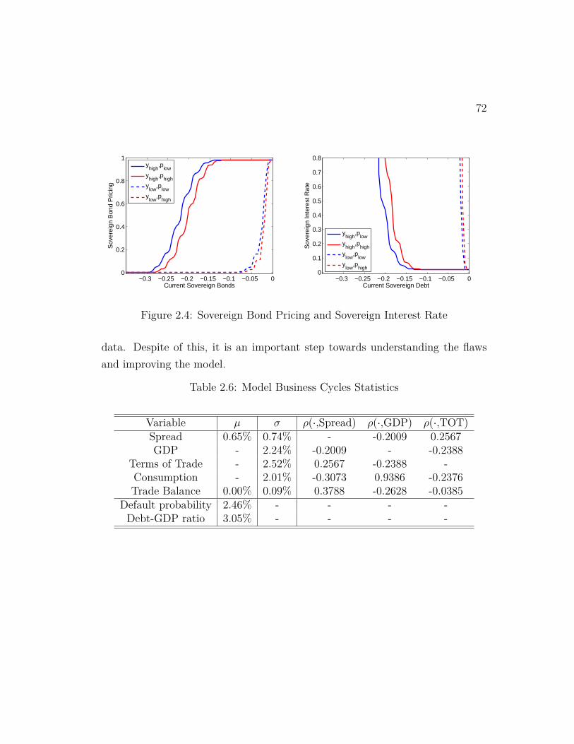
72

−0.3 −0.25 −0.2 −0.15 −0.1 −0.05 00

0.2

0.4

0.6

0.8

1

Current Sovereign Bonds

Sov

erei

gn B

ond

Pric

ing

yhigh

,plow

yhigh

,phigh

ylow

,plow

ylow

,phigh

−0.3 −0.25 −0.2 −0.15 −0.1 −0.05 00

0.1

0.2

0.3

0.4

0.5

0.6

0.7

0.8

Current Sovereign Debt

Sov

erei

gn In

tere

st R

ate

yhigh

,plow

yhigh

,phigh

ylow

,plow

ylow

,phigh

Figure 2.4: Sovereign Bond Pricing and Sovereign Interest Rate

data. Despite of this, it is an important step towards understanding the flawsand improving the model.

Table 2.6: Model Business Cycles Statistics

Variable µ σ ρ(·,Spread) ρ(·,GDP) ρ(·,TOT)Spread 0.65% 0.74% - -0.2009 0.2567GDP - 2.24% -0.2009 - -0.2388

Terms of Trade - 2.52% 0.2567 -0.2388 -Consumption - 2.01% -0.3073 0.9386 -0.2376Trade Balance 0.00% 0.09% 0.3788 -0.2628 -0.0385

Default probability 2.46% - - - -Debt-GDP ratio 3.05% - - - -

73

2.6 Conclusion

We propose a stochastic general equilibrium model of sovereign default withendogenous default risk in order to explain the interest rate behavior in emergingeconomies. We incorporate two types of shocks to cover a foreign and a domesticuncertainty. We define as the domestic and the foreign uncertainty, GDP andterms of trade shock, respectively. The model is able to succesfully increasethe dispersion of sovereign interest rates when GDP shocks are above the trend.This result seems to suggest that terms of trade is a good candidate to explainthe volatility of interest rates in small open economies when they are not underrecessions or crises.

Unfortunately, our business cycles exercise have room for improvements. Nev-ertheless, the results presented is a great step to explain the behavior of interestrates in emerging economies. Below, we present three issues we are currentlyworking in order to improve our line of research.

Firstly, the VAR(1) process does not capture correctly the dynamics betweenGDP and terms of trade shown in the data. This can be shown by the smallcorrelation between their contemporaneous realizations in the simulation process.In particular, we are confident that E [εyt |ln pt] 6= 0, making our estimators in Abiased. Moreover, we are not implementing completely the exogeneity assumptionof terms of trade. Specifically, we let the future realization of terms of trade beaffected by the current level of GDP. Furhter work of the model will considerimprovements in the VAR(1) process presented in (2.1), for example

ln yt+1

ln pt+1

=a1 a2

0 a3

ln ytln pt

+1 b1

0 1

εyt−1

εpt=1

.

74

Another weakness of our results is our calibration strategy. We let the toler-ance in the algorithm to be high for a faster convergence. The tolerance providedis of 1.0e−1, which yields really loose results. Moreover, we only do one simula-tion process in order to compute the target statistics of default probability andstandard deviation of trade balance over GDP. Future improvements will encom-pass a more serious calibration process with a higher tolerance and number ofsimulation processes. Moreover, we will include as part of it the probability ofre-entry to financial markets by targeting the ratio of debt over GDP.

Finally, our computation of the equilibrium can improve greatly. Unfortu-nately, having three state variables increases greatly the computational cost interms of time. Because of this we have coarse grids that might miss importantmovements. Furthermore, as noted by Hatchondo, Martinez and Sapriza (2010),grid search methods can yield spurious results in the business cycles statitics ofthe model. Future improvements will work on this by imposing finer grids inthe state variables. In addition, we will move from the grid search method tomethods that are able to capture movements between the grid elements23.

23There are a great variety of methods that allow movements inside the grid elements. Inparticular, we are currently working on linear and quadratic interpolation methods. We are alsointerested in implementing innovative methods that have shown effiency in solving these typesof models. Specifically, we are interested in the alogorithms provided in McGrattan (1996) andGordon and Qiu (2015).

Chapter 3

Optimal foreign currency debtdenomination

3.1 Introduction

The popular question regarding debt currency denomination is whether itshould be incurred in domestic or foreign currency. This question has been stud-ied extensively regarding private and sovereign governments, focusing in the ben-efits and shortcomings from issuing debt in a currency different to the domesticcurrency. For example, Du and Schreger (2015) study the patters of sovereigndebt in domestic and foreign currency across time. However, not all foreign cur-rencies are the same, and this dimension is missing in the literature. The questionI address in this paper is, what type of foreign currency should a country issuedebt? In particular, should a country issue debt in its trade partner currency? Ifind that as an economy falls into a recession and more debt issuance is desired,

75

76

issuing debt in a currency not linked to its trading partner currencies becomesattractive.

3.2 Two Period Model

Consider a two period small open economy inhabited with a representativefirm, a representative household, and a benevolent government. There are twodifferent type of foreign goods. One of the foreign goods is linked with the tradein the small open economy has. The real exchange rate between this foreign goodand the domestic produced good will be the terms of trade p. On the other hand,the other foreign good is not linked to the trade in the small open economy. Thereal exchange rate between this foreign and the domestic produced goods can bedescribed by e. In the first period there is no uncertainty and the terms of tradeand the real exchange rate start at their long-run level p and e, respectively. Forsimplicity, I will assume these long-run levels are the same and normalized toone. Nevertheless, in the second period there is uncertainty regarding both, theterms of trade p and the real exchange rate e.

3.2.1 Representative Household

The representative household maximizes its two period utility by consumingfinal goods. Every period, the total disposable income of the household comesfrom the profits of representative firm and a lump-sum tax/transfer by the gov-ernment. The utility maximization problem of the household can be expressed

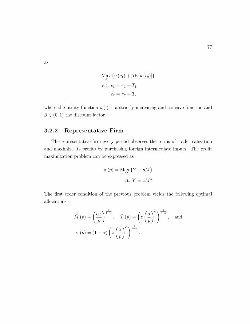
77

as

Maxc{u (c1) + βE [u (c2)]}

s.t. c1 = π1 + T1

c2 = π2 + T2

where the utility function u (·) is a strictly increasing and concave function andβ ∈ (0, 1) the discount factor.

3.2.2 Representative Firm

The representative firm every period observes the terms of trade realizationand maximize its profits by purchasing foreign intermediate inputs. The profitmaximization problem can be expressed as

π (p) = MaxY,M{Y − pM}

s.t. Y = zMα

The first order condition of the previous problem yields the following optimalallocations

M (p) =(αz

p

) 11−α

, Y (p) =(z

(α

p

)α) 11−α

, and

π (p) = (1− α)(z

(α

p

)α) 11−α

.

78

3.2.3 Foreign International Lenders

The foreign international lenders can invest in a world risk-free asset and intwo different risky government bonds in the first period. For simplicity, I assumethat the risk-free asset and one of the risky government bonds are denominatedin the same foreign good. The other risky government bond will be denominatedin the foreign good the small open economy has a trade relationship with. Theinternational lenders have deep pockets in the first period and are assumed tobe risk-neutral. The maximization problem of the international lenders can bedescribed as

Max{x1 + 1

1 + rex2

}s.t. x1 = I − qebe − qpbp

x2 = Ep,e[(1− de)be + (1− dp)

p

ebp

],

where the de and dp represent if the government default in the risky bond in thesecond period. The first order conditions of this problem yield the following debtpricing rules

qe = 11 + re

E [(1− de)] and qp = 11 + re

E[(1− dp)

p

e

].

3.2.4 Benevolent Government

The government is benevolent with respect of the representative household’swelfare and issues debt b in the first period and in the second period chooseseither to default or repay it. The government issues new debt in the first periodand it can choose whether to issue debt in the currency of its trade partner (real

79

exchange rate of p) or in a different independent currency (real exchange rateof e). If it defaults in the second period, it will receive a penalty of κ ∈ (0, 1)tradabale goods over the total profits of the representative firm. Finally, thegovernment starts with an initial amount of debt to be paid in final goods b0.The maximization problem in the first period of the benevolent government canbe summarized in

V (b0) = Max {Vp(b0), Ve(b0)} , (3.1)

where Vp(b0) and Ve(b0) represent the environment of choosing foreign denomi-nated debt in the trade partner currency or the independent currency, respec-tively. The maximization problem when debt is in the trade partner currencycan be expressed as

Vp(b0) = Maxc1,c2,b

{u (c1) + βEp [u (c2)]}

s.t. c1 + b0 = π (p) + qp (b) b

c2 =

π (p)− pb if repays

(1− κ)π (p) if defaults

80

On the other hand, the maximization problem when debt is in the an independentforeign currency can be expressed as

Ve(b0) = Maxc1,c2,b

{u (c1) + βEp,e [u (c2)]}

s.t. c1 + b0 = π (p) + qe (b) b

c2 =

π (p)− eb if repays

(1− κ)π (p) if defaults

3.2.5 Equilibrium

Let us describe the default sets for both problems as

Dp(b) ≡ {p ∈ R+ : u ((1− κ)π(p)) > u (π(p)− pb)} and (3.2)

De(b) ≡{

(p, e) ∈ R2+ : u ((1− κ)π(p)) > u (π(p)− eb)

}. (3.3)

Using these sets, we can rewrite the debt pricing as

qp(b) = 11 + re

∫ ∫p∈Dp(b)

p

edF (p)dF (e) and (3.4)

qe(b) = 11 + re

∫(p,e)∈De(b)

dF (p, e). (3.5)

81

Moreover, we can define the second period discounted expected utility as

Vp(b) ≡ βEp [u(c2)]

= β

[∫p∈Dp(b)

u(π(p)− pb)dF (p) +∫p/∈Dp(b)

u((1− κ)π(p))dF (p)]

and

Ve(b) ≡ βEp,e [u(c2)]

= β

[∫(p,e)∈De(b)

u(π(p)− eb)dF (p, e) +∫

(p,e)/∈De(b)u((1− κ)π(p))dF (p, e)

].

Figure 3.1 shows these relationships and how they change when higher debt isissued in the first period. Figure 3.1(a) shows us that for low levels of debt, thereis a higher price for debt issued in the trading partner currency. Nevertheless,this changes as higher debt starts to be issued. This can be explained as themore likely the government is to default, a negative terms of trade shock makesprofits fall and debt to rise, making default attractive when debt is issued in thetrade partner currency. Nevertheless, when debt is issued in a different foreignexchange rate, when terms of trade deteriorate, profits fall but debt does notnecessarily increases. As a matter of fact, the exchange rate may appreciate,making the debt burden fall and making default not as attractive. Figure 3.1(b)shows the discounted expected utility from the second period. It also shows thatas debt increases and comes closer to default, issuing debt in a foreign currencynot linked to the trade partner is more attractive due to the possibility of anappreciation of the currency, making the debt burden in the second period tofall.

Using these definitions, I state the following definition for a recursive equilib-rium of the two period model.

82

(a) Debt pricing

0.00 0.01 0.02 0.03 0.04 0.050.00

0.25

0.50

0.75

1.00

Trading partner currencyIndependent foreign currency

(b) Discounted expected value

0.00 0.01 0.02 0.03 0.04 0.05-13

-12

-11

-10

Trading partner currencyIndependent foreign currency

Figure 3.1: Debt pricing and second period discounted expected value contingentin debtNote: To construct these functions contingent to debt I use the parameters established in thefollowing section. The debt axis is regarding the debt incurred in the first period.

83

Definition 9 (Recursive Equilibrium) A recursive equilibrium with initialdebt b0 is defined as value functions {V (b0), Vp(b0), Ve(b0)}, a set of debt pricingschedules {qp(b), qe(b)}, and default sets {Dp(b),De(b)}; such that the followingconditions are satisfied:

1. The decision of whether to issue debt in the trade partner currency or adifferent foreign currency satisfies (3.1).

2. Taking the debt pricing schedule qp(b), the following problem is solved

Vp(b0) = Maxb{u (π (p) + qp (b) b− b0) + Vp(b)} .

3. Taking the debt pricing schedule qe(b), the following problem is solved

Ve(b0) = Maxb{u (π (p) + qe (b) b− b0) + Ve(b)} .

4. The default sets satisfy (3.2) and (3.3).

5. The debt pricing schedules satisfy (3.4) and (3.5).

3.3 Quantitative Analysis

In this section, I pick the functional forms and values to the parameters of themodel. I solve for both currencies a grid search method to find the optimal debt.Then I choose the the currency that yields the highest utility in the first periodgiven an initial debt paid in the first period. I then study how the currency choicechange as the initial debt increases.

84

3.3.1 Baseline Calibration

I calibrate the model taking parameters values widely accepted in the litera-ture. I discretize the initial debt, the period 1 debt, and the terms of trade spaceinto grids of 5001 elements each. For the grids regarding debt, the elements aregoing to be equally separated from 0.0 to 0.1. For the terms of trade, I followTauchen and Hussey (1991) to obtain the probability transition matrix and theelements of the grid for an AR(1) process. For the stochastic process of the dif-ferent exchange rate, I take set it to take only two values in such a way thatthe average of the exchange rate shock is the long-run level of the terms of tradeshock.

Functional Forms. The utility function is a standard CRRA

u(c) = c1−γ

1− γ ,

where γ represents the risk aversion parameter of the households.I assume a decreasing returns to scale production function

F (M) = zMα,

where α < 1.I assume the log terms of trade process follow an AR(1) process

ln (p′) = ρ ln(p) + σε

where the auto-correlation parameter satisfy |ρ|< 0, and the shocks are i.i.d. and

85

normal distributed, ε ∼ N(0, 1).Finally, I assume that the real exchange rate follow a Bernoulli distribution

with parameter λ. I also set that the mean of the exchange rate coincides withthe long-run level of the terms of trade shock.

Model Parameters. Table 3.1 shows all the baseline calibration values forthe parameters of the model. I set values of the parameters widely used in theliterature. I normalize the productivity of the final good production as well as thelong-run level of the log terms of trade stochastic process. Its auto-correlationand standard deviation are consistent to the values found in the literature.

Table 3.1: Calibration table

Parameter Valuep 1.00e 1.00z 1.00αM 0.75γ 2.00λ 0.80ρ 0.50σ 0.08r 1.01β 0.99

Figure 3.2 show the optimal debt of the sovereign government contingent toan initial debt the government needs to pay in the first period. This can alsobe seen as a contraction in the economy measuring an initial crisis in the firstperiod. This makes the government incur in more debt and therefore more close

86

to a default scenario in the second period. Figure 3.2(a) show the optimal debtincurred in each type of foreign currency denomination. Figure 3.2(b) portraysthe same curves but considering considering when it is optimal to incur the debtin the trading partner currency or not. The main message of the model is thatthe higher debt is needed in the first period, issuing debt in a different currencybecomes more attractive. The figure shows that for initial debt levels of 0.72,debt in the trading partner currency is optimal. However, for higher levels ofinitial debt, the government will find more attractive to issue debt in a currencynot linked to its terms of trade.

(a) Optimal debt

0.00 0.02 0.04 0.06 0.08 0.10

0.005

0.010

0.015

0.020

0.025

(b) Optimal currency

0.00 0.02 0.04 0.06 0.08 0.10

0.005

0.010

0.015

0.020

0.025

Figure 3.2: Optimal debt issuance contingent to initial debt

3.4 Conclusion

In this paper, I deviate from the question of whether a country should issuedebt in domestic or foreign currency. Instead I focus in the question of what

87

type of foreign currency should a country issue its debt. To answer this questionI create a two period model where a sovereign government chooses whether toissue debt in a currency tied to their terms of trade or not. I find that when agovernment is not in a recession, a government is more prone to choose a foreigncurrency linked to their trading patterns. Nevertheless, as soon as a governmentis in a recession and needs to incur in higher levels of debt, changing to a currencynot linked to its trading patterns becomes more attractive. This is due to theprobability of the domestic currency to appreciate and contract the debt burdenwhen there is a deterioration in the terms of trade.

Bibliography

Aguiar, Mark and Gopinath, Guita. (2007), The role of interest rates andproductivity shocks in emerging market fluctuations.

Alessandro, Mauro, Sandleris, Guido and Van Der Ghote, Alejandro.(2011). ‘Sovereign defaults and the political economy of market reaccess’.

Arellano, Cristina. (2008). ‘Default risk and income fluctuations in emergingeconomies’, The American Economic Review 98(3), 690–712.

Asonuma, Mr Tamon. (2016), Sovereign defaults, external debt, and real ex-change rate dynamics, International Monetary Fund.

Benguria, Felipe, Saffie, Felipe and Urzúa, Sergio. (2018). ‘The transmis-sion of commodity price super-cycles’.

Broda, Christian. (2004). ‘Terms of trade and exchange rate regimes in devel-oping countries’, Journal of International economics 63(1), 31–58.

Chatterjee, Satyajit, Corbae, Dean, Nakajima, Makoto and Rios-Rull,Jose-Victor. (2007). ‘A quantitative theory of unsecured consumer creditwith risk of default’, Econometrica 75(6), 1525–1589.

88

89

Chatterjee, Satyajit and Eyigungor, Burcu. (2012). ‘Maturity, indebted-ness, and default risk’, The American Economic Review 102(6), 2674–2699.

Cole, Harold and Kehoe, Timothy. (1996). ‘A self-fulfilling model of Mexico’s1994–1995 debt crisis’, Journal of International Economics 41(3), 309–330.

Conesa, Juan Carlos, Kehoe, Timothy J and Ruhl, Kim J. (2007). ‘Mod-eling great depressions: the depression in Finland in the 1990s’.

Costa, Daniela. (2017), Essays in international economics and labor economics,PhD thesis, University of Minnesota.

Cuadra, Gabriel and Nuguer, Victoria. (2016). ‘Risky banks and macro-prudential policy for emerging economies’.

Cuadra, Gabriel and Sapriza, Horacio. (2006). ‘Sovereign default, terms oftrade, and interest rates in emerging markets’.

De Gregorio, Jose andWolf, Holger C. (1994). ‘Terms of trade, productivity,and the real exchange rate’.

de Soyres, François. (2016). ‘Value added and productivity linkages acrosscountries’, Toulouse School of Economics .

Du, Wenxin and Schreger, Jesse. (2015). ‘Sovereign risk, currency risk, andcorporate balance sheets’, Harvard, Department of Economics Working Paper.

Easterly, William, Islam, Roumeen and Stiglitz, Joseph E. (2001),Shaken and stirred: explaining growth volatility, in ‘Annual World Bank con-ference on development economics’, Vol. 2000, pp. 191–211.

90

Eaton, Jonathan and Gersovitz, Mark. (1981). ‘Debt with potential repu-diation: Theoretical and empirical analysis’, The Review of Economic Studies48(2), 289–309.

Eichengreen, Barry and Hausmann, Ricardo. (1999). ‘Exchange rates andfinancial fragility’.

Gelos, Gaston, Sahay, Ratna and Sandleris, Guido. (2011). ‘Sovereignborrowing by developing countries: What determines market access?’, Journalof international Economics 83(2), 243–254.

Gordon, Grey and Qiu, Shi. (2015). ‘A divide and conquer algorithm forexploiting policy function monotonicity’, SSRN 2556345 .

Greenwood, Jeremy, Hercowitz, Zvi and Huffman, Gregory W. (1988).‘Investment, capacity utilization, and the real business cycle’, The AmericanEconomic Review pp. 402–417.

Gu, Grace. (2015). ‘A tale of two countries: sovereign default, exchange rate,and trade’.

Hatchondo, Juan Carlos and Martinez, Leonardo. (2009). ‘Long-durationbonds and sovereign defaults’, Journal of International Economics 79(1), 117–125.

Hatchondo, Juan Carlos, Martinez, Leonardo and Sapriza, Horacio.(2010). ‘Quantitative properties of sovereign default models: solution methodsmatter’, Review of Economic dynamics 13(4), 919–933.

91

Jeanne, Olivier. (2003), Why do emerging economies borrow in foreign cur-rency?, number 3-177, International Monetary Fund.

Kehoe, Timothy and Ruhl, Kim. (2008). ‘Are shocks to the terms of tradeshocks to productivity?’, Review of Economic Dynamics 11(4), 804–819.

King, Robert G, Plosser, Charles I and Rebelo, Sergio T. (1988). ‘Pro-duction, growth and business cycles: I. The basic neoclassical model’, Journalof monetary Economics 21(2-3), 195–232.

Kose, Ayhan, Towe, Christopher and Meredith, Guy. (2004), How hasNAFTA affected the Mexican economy? Review and evidence, number 4-59,International Monetary Fund.

Kose, M Ayhan. (2002). ‘Explaining business cycles in small openeconomies:?How much do world prices matter??’, Journal of International Eco-nomics 56(2), 299–327.

McGrattan, Ellen R. (1996). ‘Solving the stochastic growth model with a finiteelement method’, Journal of Economic Dynamics and Control 20(1), 19–42.

Mendoza, Enrique G. (1991). ‘Real business cycles in a small open economy’,The American Economic Review pp. 797–818.

Mendoza, Enrique G. (1995). ‘The terms of trade, the real exchange rate, andeconomic fluctuations’, International Economic Review pp. 101–137.

Mendoza, Enrique G. (1997). ‘Terms of trade uncertainty and economicgrowth’, Journal of Development Economics 54(2), 323–356.

92

Mendoza, Enrique and Yue, Vivian. (2011). ‘A general equilibrium modelof sovereign default and business cycles’.

Na, Seunghoon, Schmitt-Grohé, Stephanie, Uribe, Martin and Yue,Vivian Z. (2014). ‘A model of the twin ds: Optimal default and devaluation’.

Neumeyer, Pablo and Perri, Fabrizio. (2005). ‘Business cycles in emerg-ing economies: the role of interest rates’, Journal of Monetary Economics52(2), 345–380.

Popov, Sergey V, Wiczer, David et al. (2014). ‘Equilibrium SovereignDefault with Exchange Rate Depreciation’, Federal Reserve Bank of St. LouisWorking Paper Series (2014-049).

Reinhart, Carmen and Rogoff, Kenneth. (2009), This time is different:eight centuries of financial folly, Princeton University Press.

Ruhl, Kims. (2008). ‘The international elasticity puzzle’, NYU (Unpublished) .

Schmitt-Grohé, Stephanie and Uribe, Martín. (2016). ‘Downward nomi-nal wage rigidity, currency pegs, and involuntary unemployment’, Journal ofPolitical Economy 124(5), 1466–1514.

Tauchen, George and Hussey, Robert. (1991). ‘Quadrature-based methodsfor obtaining approximate solutions to nonlinear asset pricing models’, Econo-metrica: Journal of the Econometric Society pp. 371–396.

Tomz, Michael and Wright, Mark. (2007). ‘Do countries default in badtimes?’, Journal of the European Economic Association 5(2-3), 352–360.

93

94

Chapter 4

Appendix

4.1 Propositions proofs

4.1.1 Proposition 4 (Recursive Equilibrium Isomorphism)

Proof Let us use this intratemporal condition (2.9) and the household’s finalconsumption aggregator,

C =(λc−ηd + (1− λ)c−ηf

)− 1η

= cd

(λ

(1 +

(1− λλ

)(cdcf

)η))− 1η

= cd

λ1 +

(1− λλ

)((λ

1− λ

)p

) η1+η−

1η

= cd

λ1 +

(1− λλ

) 11+η

pη

1+η

−1η

=(

cd

λ1

1+η

)(λ

11+η + (1− λ)

11+η p

η1+η)− 1

η.

95

Using the final consumption good price index (2.10), we can rewrite the previousexpression as

c1+ηd

λ= P(p)C1+η. (4.1)

Using the the intratemporal condition (2.9) and mixing the budget and the bal-anced trade constraints of (2.4) and (2.5), we can realise that the consumptionof domestic and foreign expenditure can be expressed as

cd + pcf = cd +(

1− λλ

)(cdcf

)1+η

cf

= cd +(

1− λλ

)c1+ηd c−ηf

=(c1+ηd

λ

)(λc−ηd + (1− λ)c−ηf

)= c1+η

d

λCη.

Thus, using (4.1) we reach the expression that the household’s consumption ex-penditure can be expressed in terms of the final consumption good and the finalconsumption good price index (2.10),

cd + pcf = P(p)C.

Furthermore, using (2.9) and (4.1), we can construct how the consumption ofdomestic and foreign goods can be decomposed from the aggregate final con-

96

sumption good as

cd = (λP(p))1

1+η C and cf =(

(1− λ)P(p)p

) 11+η

C.

Finally, realise that the restrictions of the maximization problems (2.4) and (2.5)are the same as the ones described in (2.11) and (2.12).

4.1.2 Proposition 5 (Default Sets Monotonicity)

Proof Set a level of sovereign debt B1 and levels of output and terms of tradesuch that (y, p) ∈ D(B1). Then, it follows that V D(y, p) > V R(B1, y, p). Pick anarbitrary level of sovereign debt B2 such that B2 ≤ B1. Let us study the resourceconstraint in (2.11). Define the budget set of the government contingent to theamount of sovereign bonds due as

B(B) = {(C,B′) ∈ R+ × [B,∞) : P (p)C + pq(B′, y, p) ≤ y + pB} .

By construction, acknowledge that B(B2) ⊆ B(B1). Because the government ismaximizing over a subset of a set, it follows that V R(B1, y, p) ≥ V R(B2, y, p).Joining the inequalities, we conclude that

V D(y, p) > V R(B1, y, p) ≥ V R(B2, y, p).

In other words, (y, p) ∈ D(B2). Finally, because the levels of sovereign debt B2

was taken arbitrarily, we can conclude that D(B1) ⊆ D(B2).

97

4.1.3 Proposition 6 (No Resources Inflows)

Proof Pick an arbitrary (y, p) ∈ D(B) and realise this implies V D(y, p) >

V R(B, y, p). Acknowledge that the resource constraints found in (2.11) and in(2.12) can be rewritten respectively as

C = y

P(p) −p

P(p) (q(B′)B′ −B) and C = y

P(p) .

Therefore,

u

(y

P(p)

)+ βE(y′,p′)

[V D(y′, p′)

]>

> MaxB′

{u

(y − p(q(B′)B′ −B)

P(p)

)+ βE(y′,p′) [V (y′, p′)]

}

≥ MaxB′

{u

(y − p(q(B′)B′ −B)

P(p)

)+ βE(y′,p′)

[V D(y′, p′)

]}

≥ u

(y − p(q(B′)B′ −B)

P(p)

)+ βE(y′,p′)

[V D(y′, p′)

],

for all feasible B′. Thus,

u

(y

P(p)

)> u

(y

P(p) −p

P(p) (q(B′)B′ −B)).

Because u(·) is an increasing function,

y

P(p) ≥y

P(p) −p

P(p) (q(B′)B′ −B) .

98

Then, we arrive to

q(B′)B′ −B ≥ 0.

Finally, because we picked an arbitrary (y, p) ∈ D(B), we can conclude that forall feasible B′ there are no resources inflows, q(B′)B′ −B ≥ 0.

4.1.4 Proposition 7 (GDP Default Incentives)

Proof Set a level of GDP, terms of trade and sovereign bonds such that (y1, p) ∈D(B) 6= ∅. Then, it follows that V D(y1, p) > V R(B, y1, p). Pick an arbitrarylevel of GDP y2 such that y2 ≤ y1. Acknowledge that the resource constraintsfound in (2.11) and in (2.12) can be rewritten respectively as

C = y

P(p) −p

P(p) (q(B′)B′ −B) and C = y

P(p) .

To make the proof easier, call

B′1 = arg MaxB′

{u

(y1

P(p) −p

P(p) (q(B′1)B′1 −B))

+ βE(y′,p′) [V (B′1, y′, p′)]}

&

B′2 = arg MaxB′

{u

(y2

P(p) −p

P(p) (q(B′2)B′2 −B))

+ βE(y′,p′) [V (B′2, y′, p′)]}.

99

Realise that, in particular, these expressions imply,

u

(y1

P(p) −p

P(p) (q(B′1)B′1 −B))

+ βE(y′,p′) [V (B′1, y′, p′)] ≥

u

(y1

P(p) −p

P(p) (q(B′2)B′2 −B))

+ βE(y′,p′) [V (B′2, y′, p′)] .

Using Proposition 6 and because D(B) 6= ∅ and u(·) is increasing, it followsthat q(B′)B′−B ≥ 0 for every feasible B′. In particular, for the optimal level ofsovereign bonds using y2 level of GDP, q(B′2)B′2 −B ≥ 0.

Because u(·) is strictly concave and q(B′2)B′2 −B ≥ 0, we know that

u

(y1

P(p) −p

P(p) (q(B′2)B′2 −B))− u

(y2

P(p) −p

P(p) (q(B′2)B′2 −B))≥

≥ u

(y1

P(p)

)− u

(y1

P(p)

).

Moreover, the right hand side can be expressed as

u

(y1

P(p)

)− u

(y2

P(p)

)=(u

(y1

P(p)

)+ βE(y′,p′) [V (y′, p′)]

)

−(u

(y2

P(p)

)+ βE(y′,p′) [V (y′, p′)]

)= V D(y1, p)− V D(y2, p).

100

Therefore,

V D(y1, p)− V D(y2, p) ≤ u

(y1

P(p) −p

P(p) (q(B′2)B′2 −B))

− u(

y2

P(p) −p

P(p) (q(B′2)B′2 −B))

=(u

(y1

P(p) −p

P(p) (q(B′2)B′2 −B))

+ βE(y′,p′) [V (B′2, y′, p′)])

−(u

(y2

P(p) −p

P(p) (q(B′2)B′2 −B))

+ βE(y′,p′) [V (B′2, y′, p′)])

≤(u

(y1

P(p) −p

P(p) (q(B′1)B′1 −B))

+ βE(y′,p′) [V (B′1, y′, p′)])

−(u

(y2

P(p) −p

P(p) (q(B′2)B′2 −B))

+ βE(y′,p′) [V (B′2, y′, p′)])

= V R(B, y1, p)− V R(B, y2, p)

< V D(y1, p)− V R(B, y2, p).

Then we arrive to following expression V D(y2, p) > V R(B, y2, p). Finally we canconclude, because the level of GDP y2 was taken arbitrarily, we can conclude that(y2, p) ∈ D(B).

4.1.5 Proposition 8 (Terms of Trade Default Incentives)

Proof Set a level of GDP, terms of trade and sovereign bonds such that (y, p1) ∈D(B) 6= ∅. Then, it follows that V D(y, p1) > V R(B, y, p1). Pick an arbitrary levelof terms of trade p2 such that p2 ≥ p1. Acknowledge that the resource constraints

101

found in (2.11) and in (2.12) can be rewritten respectively as

C = y

P(p) −p

P(p) (q(B′)B′ −B) and C = y

P(p) .

To make the proof easier, call

B′1 = arg MaxB′

{u

(y

P(p1) −p1

P(p1) (q(B′1)B′1 −B))

+ βE(y′,p′) [V (B′1, y′, p′)]}

&

B′2 = arg MaxB′

{u

(y

P(p2) −p2

P(p2) (q(B′2)B′2 −B))

+ βE(y′,p′) [V (B′2, y′, p′)]}.

Realise that, in particular, these expressions imply,

u

(y

P(p1) −p1

P(p1) (q(B′1)B′1 −B))

+ βE(y′,p′) [V (B′1, y′, p′)] ≥

u

(y

P(p1) −p1

P(p1) (q(B′2)B′2 −B))

+ βE(y′,p′) [V (B′2, y′, p′)] .

Using Proposition 6 and because D(B) 6= ∅ and u(·) is increasing, it followsthat q(B′)B′−B ≥ 0 for every feasible B′. In particular, for the optimal level ofsovereign bonds using y2 level of GDP, q(B′2)B′2 −B ≥ 0.

Acknowledge that the final consumption good price index is increasing,

P ′(p) =(

(1− λ)P(p)p

) 11+η

≥ 0.

102

Therefore, the ratio pP(p) is increasing too,

d

dp

(p

P(p)

)= P(p)− pP ′(p)

(P(p))2

= 1− (1− λ)1

1+η pη

1+η (P(p))−η

1+η

P(p)

= (P(p))η

1+η − (1− λ)1

1+η pη

1+η

(P(p))1+2η1+η

=(

λ

(P(p))1+2η

) 11+η

≥ 0.

In other words, it follows that p2P(p2) ≥

p1P(p1) because p2 ≥ p1.

Using the previous result and because u(·) is strictly concave andq(B′2)B′2 −B ≥ 0, we know that

u

(y

P(p1)

)− u

(y

P(p2)

)≤ u

(y

P(p1) −p2

P(p2) (q(B′2)B′2 −B))

− u(

y

P(p2) −p2

P(p2) (q(B′2)B′2 −B))

≤ u

(y

P(p1) −p1

P(p1) (q(B′2)B′2 −B))

− u(

y

P(p2) −p2

P(p2) (q(B′2)B′2 −B))

103

Moreover, the left hand side can be expressed as

u

(y

P(p1)

)− u

(y

P(p2)

)=(u

(y

P(p1)

)+ βE(y′,p′) [V (y′, p′)]

)

−(u

(y

P(p2)

)+ βE(y′,p′) [V (y′, p′)]

)= V D(y, p1)− V D(y, p2).

Therefore,

V D(y, p1)− V D(y, p2) ≤

≤ u

(y

P(p1) −p1

P(p1) (q(B′2)B′2 −B))− u

(y

P(p2) −p2

P(p2) (q(B′2)B′2 −B))

=(u

(y

P(p1) −p1

P(p1) (q(B′2)B′2 −B))

+ βE(y′,p′) [V (B′2, y′, p′)])

−(u

(y

P(p2) −p2

P(p2) (q(B′2)B′2 −B))

+ βE(y′,p′) [V (B′2, y′, p′)])

≤(u

(y

P(p1) −p1

P(p1) (q(B′1)B′1 −B))

+ βE(y′,p′) [V (B′1, y′, p′)])

−(u

(y

P(p2) −p2

P(p) (q(B′2)B′2 −B))

+ βE(y′,p′) [V (B′2, y′, p′)])

= V R(B, y, p1)− V R(B, y, p2)

< V D(y, p1)− V R(B, y, p2).

Then we arrive to following expression V D(y, p2) > V R(B, y, p2). Finally we canconclude, because the level of terms of trade p2 was taken arbitrarily, we canconclude that (y, p2) ∈ D(B).

104

4.2 Computational algorithm

We extend the algoritm described in Arellano (2008) and incorporate the oneloop enhancement proposed in Hatchondo, Martinez and Sapriza (2010) using agrid search method. The following is the algorithm we follow to solve the modelproposed in Definition 3 and the calibration strategy for the discount factor βand the GDP default penalty parameter κ:

1) Fix the calibration targets of default probability d and standard deviationof trade balance over GDP s.

2) Discretize B space and dicretize (y,p) space using Tauchen and Hussey(1991)

3) Propose a guess for the discount factor β and the GDP default penaltyparameter κ,

β = 0.95 andκ = 1.00

4) Propose a guess for the set of value functions V , V R, V D and the sovereignbond price schedule q,

V = [0], V R = [0], V D = [0], and q =[ 11 + r∗

].

5) For every state (B, y, p), solve the repayment state maximization problem(2.11) and compute an implied repayment state value function V R.

6) For every state (y, p), solve the repayment state maximization problem(2.12) and compute an implied default state value function V D.

105

7) For every state (B, y, p), solve the maximization problem and compute animplied default state value function V .

8) Using the implied value functions V R and V D, construct default set D

9) Using the default set D, construct default probability schedule δ

10) Using the default probability schedule δ, construct an implied sovereignbond price schedule q

11) Compute the error term as

z1 = ||V − V ||∞+||V R − V R||∞+||V D − V D||∞+||q − q||∞.

12) Update guesses V = V , V R = V R, V D = V D, and q = q.

13) If z1 ≥ 1.0e−6, return to 5).

14) Construct one simulation of 10,000 periods with 500 burn-ins starting withthe zero sovereign bonds and the long-run levels of GDP and terms of trade

15) Construct the implied default probability α and the implied standard de-viation of trade balance over GDP s

16) Compute the error term as

z2 =

∣∣∣d− d∣∣∣+ |s− s|2 .

17) If z2 ≥ 1.0e−1, update guesses β and κ, then return to 4)