PROGRESS-VARIABLE APPROACH FOR LARGE-EDDY

SIMULATION OF TURBULENT COMBUSTION

a dissertation

submitted to the department of mechanical engineering

and the committee on graduate studies

of stanford university

in partial fulfillment of the requirements

for the degree of

doctor of philosophy

Charles David Pierce

June 2001

c© Copyright 2001 by Charles David Pierce

All Rights Reserved

– ii –

I certify that I have read this dissertation and that in

my opinion it is fully adequate, in scope and in quality,

as a dissertation for the degree of Doctor of Philosophy.

Parviz Moin (Principal Advisor)

I certify that I have read this dissertation and that in

my opinion it is fully adequate, in scope and in quality,

as a dissertation for the degree of Doctor of Philosophy.

Craig T. Bowman

I certify that I have read this dissertation and that in

my opinion it is fully adequate, in scope and in quality,

as a dissertation for the degree of Doctor of Philosophy.

Godfrey Mungal

Approved for the University Committee on Graduate

Studies:

– iii –

– iv –

ABSTRACT

A new approach to chemistry modeling for large eddy simulation of turbulent react-

ing flows is developed. Instead of solving transport equations for all of the numerous

species in a typical chemical mechanism and modeling the unclosed chemical source

terms, the present study adopts an indirect mapping approach, whereby all of the

detailed chemical processes are mapped to a reduced system of tracking scalars.

Presently, only two such scalars are considered: a mixture fraction variable, which

tracks the mixing of fuel and oxidizer, and a progress variable, which tracks the

global extent-of-reaction of the local mixture. The mapping functions, which de-

scribe all of the detailed chemical processes with respect to the tracking variables,

are determined by solving quasi-steady diffusion-reaction equations with complex

chemical kinetics and multicomponent mass diffusion. The performance of the new

model is compared to fast chemistry and steady flamelet models for predicting ve-

locity, species concentration, and temperature fields in a methane-fueled coaxial

jet combustor for which experimental data are available. The progress-variable

approach is able to capture the unsteady, lifted flame dynamics observed in the

experiment, and to obtain good agreement with the experimental data and sig-

nificantly outperform the fast chemistry and steady flamelet models, which both

predict an attached flame.

– v –

– vi –

ACKNOWLEDGEMENTS

Financial support for this work was provided by the Air Force Office of Scientific

Research under grant F49620-95-1-0185 and by the Franklin P. and Caroline M.

Johnson Fellowship. Computer resources were provided by NASA-Ames Research

Center through the Center for Turbulence Research and by the Department of

Energy’s ASCI program.

This work has benefited greatly from discussions with many graduate students,

postdoctoral fellows, professors, and visitors at the Center for Turbulence Research,

among them, Knut Akselvoll, Blair Perot, Tom Bewley, Artur Kravchenko, Robert

Jacobs, Jason Rife, Cliff Wall, Tom Lund, Hans Kaltenbach, Ken Jansen, Mas-

similiano Fatica, Kendal Bushe, Franck Nicoud, Joe Oefelein, Heinz Pitsch, Bill

Reynolds, Tom Bowman, Amable Linan, Javier Jimenez, Luc Vervisch, Thierry

Poinsot, Fokian Egolfopoulos, Bob Bilger, George Kosaly, and Norbert Peters.

I would especially like to thank my advisor, Professor Parviz Moin, for indoc-

trinating me into the ways of science, turbulence, and computer simulations, for his

steadfast support, limitless patience, and encouragement that he has given to me

and his other students, and for his commitment to excellence in research. I would

also like to thank my reading committee members, Professors Tom Bowman and

Godfrey Mungal, for their helpful comments on a draft of this dissertation.

– vii –

– viii –

TABLE OF CONTENTS

Abstract . . . . . . . . . . . . . . . . . . . . . . . . . . . . . . v

Acknowledgements . . . . . . . . . . . . . . . . . . . . . . . . . . vii

List of Figures . . . . . . . . . . . . . . . . . . . . . . . . . . . . xi

Nomenclature . . . . . . . . . . . . . . . . . . . . . . . . . . . xiii

1. Introduction

1.1 Motivation and Objective . . . . . . . . . . . . . . . . . . . 1

1.2 Literature Survey . . . . . . . . . . . . . . . . . . . . . . . 3

1.3 Accomplishments . . . . . . . . . . . . . . . . . . . . . . . 6

2. Governing Equations

2.1 The Equations of Gaseous Combustion . . . . . . . . . . . . . 9

2.2 Simplifying Assumptions . . . . . . . . . . . . . . . . . . . 10

2.3 Working Equation Set . . . . . . . . . . . . . . . . . . . . 14

3. Turbulence and Chemistry Models

3.1 Filtering and the LES Equations . . . . . . . . . . . . . . . . 17

3.2 Subgrid-Scale Models . . . . . . . . . . . . . . . . . . . . . 18

3.2.1 The Dynamic Procedure . . . . . . . . . . . . . . . . . 18

3.2.2 Turbulent Stress and Scalar Flux . . . . . . . . . . . . . 21

3.2.3 Variance and Dissipation Rate of a Conserved Scalar . . . . 23

3.2.4 Assumed Beta PDF for a Conserved Scalar . . . . . . . . . 24

3.3 Chemistry Models . . . . . . . . . . . . . . . . . . . . . . 26

3.3.1 The Role of Mixture Fraction . . . . . . . . . . . . . . 26

3.3.2 Fast Chemistry Assumption . . . . . . . . . . . . . . . 29

3.3.3 Classical Steady Flamelets . . . . . . . . . . . . . . . . 31

3.3.4 The Flamelet/Progress-Variable Approach . . . . . . . . . 40

4. Numerical Methods

4.1 Conservative Space-Time Discretization . . . . . . . . . . . . . 51

4.1.1 The Role of Conservation . . . . . . . . . . . . . . . . 51

– ix –

4.1.2 Index-Free Notation . . . . . . . . . . . . . . . . . . . 52

4.1.3 Fully Discrete Equations . . . . . . . . . . . . . . . . . 54

4.1.4 Benefits of Staggering . . . . . . . . . . . . . . . . . . 55

4.1.5 Discrete Conservation Properties . . . . . . . . . . . . . 57

4.1.6 Spurious Heat Release . . . . . . . . . . . . . . . . . . 58

4.2 Iterative Semi-Implicit Scheme . . . . . . . . . . . . . . . . . 59

4.3 Scalar Advection . . . . . . . . . . . . . . . . . . . . . . . 65

4.4 Cylindrical Coordinates . . . . . . . . . . . . . . . . . . . . 67

4.4.1 Discrete Equations in Cylindrical Coordinates . . . . . . . 67

4.4.2 Centerline Treatment . . . . . . . . . . . . . . . . . . 69

4.4.3 Exact Representation of Uniform Flow . . . . . . . . . . 70

4.5 Boundary Conditions . . . . . . . . . . . . . . . . . . . . . 70

4.5.1 Wall Boundaries . . . . . . . . . . . . . . . . . . . . 71

4.5.2 Inflow Conditions . . . . . . . . . . . . . . . . . . . . 72

4.5.3 Outflow Conditions . . . . . . . . . . . . . . . . . . . 74

5. Application to a Coaxial Jet Combustor

5.1 Experimental Configuration . . . . . . . . . . . . . . . . . . 77

5.2 Computational Setup . . . . . . . . . . . . . . . . . . . . . 79

5.3 Results . . . . . . . . . . . . . . . . . . . . . . . . . . . 82

5.3.1 Chemistry Model Comparison . . . . . . . . . . . . . . 83

5.3.2 Importance of Differential Diffusion . . . . . . . . . . . . 88

6. Conclusions and Future Directions

6.1 Conclusions . . . . . . . . . . . . . . . . . . . . . . . . . 97

6.2 Recommendations for Future Work . . . . . . . . . . . . . . . 98

References . . . . . . . . . . . . . . . . . . . . . . . . . . . . . 101

– x –

LIST OF FIGURES

3.1 Temperature as a function of mixture fraction from equilibrium

and fast chemistry state relationships. . . . . . . . . . . . . . 31

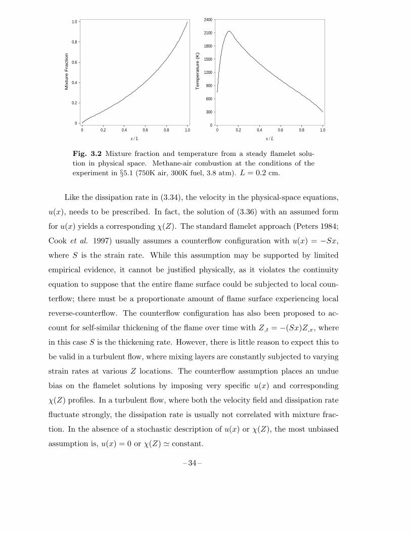
3.2 Mixture fraction and temperature from a steady flamelet solution

in physical space. . . . . . . . . . . . . . . . . . . . . . . 34

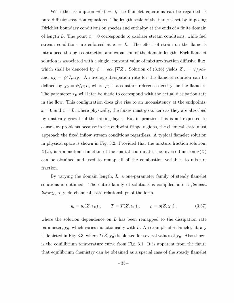
3.3 A family of solutions for the steady, one-dimensional, diffusion-

reaction equations, mapped to mixture fraction. . . . . . . . . . 36

3.4 Locus of maximum flame temperatures in the steady flamelet

library. . . . . . . . . . . . . . . . . . . . . . . . . . . . 38

3.5 Effect of the log-normal distribution on the flamelet library. . . . . 39

3.6 Locus of maximum flame temperatures from a complete set of

steady flamelet solutions including the unstable branch. . . . . . . 46

3.7 Locus of maximum flame temperatures viewed as reaction rate

versus temperature. . . . . . . . . . . . . . . . . . . . . . 47

4.1 A staggered space-time grid. . . . . . . . . . . . . . . . . . . 54

4.2 Modified wavenumber diagram for second order central differ-

ences based on stencil widths of 2∆ and ∆. . . . . . . . . . . . 56

4.3 Linear stability regions for 1, 2, and 3 iterations. . . . . . . . . . 61

4.4 Numerical dispersion of a Gaussian bump after being advected

to the right a distance of one unit. . . . . . . . . . . . . . . . 66

4.5 Staggered grid with cylindrical coordinates. . . . . . . . . . . . 67

4.6 Staggered grid at a wall boundary. . . . . . . . . . . . . . . . 71

5.1 Schematic of the coaxial jet combustor experiment. . . . . . . . . 78

5.2 Schematic of the grid used for the simulations. . . . . . . . . . . 80

5.3 Snapshot of mixture fraction in a meridional plane. . . . . . . . . 90

5.4 Snapshot of product mass fraction in a meridional plane. . . . . . 91

5.5 Radial profiles of time-averaged mixture fraction. . . . . . . . . 92

5.6 Radial profiles of time-averaged product mass fraction. . . . . . . 92

– xi –

5.7 Radial profiles of time-averaged temperature. . . . . . . . . . . 93

5.9 Radial profiles of time-averaged CO mass fraction. . . . . . . . . 94

5.8 Radial profiles of time-averaged axial velocity and axial fluctua-

tion intensity. . . . . . . . . . . . . . . . . . . . . . . . . 94

5.11 Radial profiles of time-averaged mixture fraction. . . . . . . . . 95

5.10 Effect of mass diffusion model on the flamelet library. . . . . . . . 95

5.12 Radial profiles of time-averaged product mass fraction. . . . . . . 96

– xii –

NOMENCLATURE

Roman Symbols

Ai atomic mass of element i

c convection velocity; dimensionless coefficient

cp mixture specific heat at constant pressure (per unit mass)

cp,i specific heat at constant pressure of species i (per unit mass)

C model coefficient; generic progress variable

Dij binary mass diffusion coefficient matrix

DT,i thermal mass diffusion coefficient of species i

DDt material derivative operator, D

Dt =∂∂t + u · ∇

e 2.71828 . . . ; mixture internal energy per unit mass

ei internal energy of species i (per unit mass)

f(. . .) generic function

fi body force per unit mass of species i

g mass flux, g = ρu

h mixture enthaply per unit mass

hi enthaply of species i (per unit mass)

I indentity tensor, Iij = δij

k kinetic energy per unit mass, k = 12u2; wavenumber

L flamelet domain length

Mi molecular mass of species i

n boundary-normal coordinate

NE number of chemical elements

NS number of chemical species

Nij number of j atoms in a molecule of species i

p pressure

p0 background pressure

P (. . .) probability density function

– xiii –

q heat flux vector

qR radiative heat flux vector

qD Dufour heat flux

qij residual scalar flux of species i

r radial coordinate

R universal gas constant

R normalizing length scale

s mixture entropy per unit mass

S strain-rate tensor, Sij =12(ui,j + uj,i)

t time

tij residual stress tensor

T temperature

u velocity component or magnitude; generic variable

u velocity vector

U normalizing velocity scale

Vi mass diffusion velocity of species i

wi chemical production rate of species i

x spatial coordinate; generic variable

xi mole fraction of species i

yi mass fraction of species i

yP product mass fraction

Z mixture fraction

Greek Symbols

α generic diffusivity

αm molecular diffusivity

αt turbulent diffusivity

αi mass diffusivity of species i

αT thermal diffusivity

αZ mixture-fraction diffusivity

– xiv –

Γ Gamma function, Γ(n) = (n− 1)!

δ Dirac delta function

δij Kronecker delta

δx(·) finite-difference operator

∆ filter width; grid spacing

η generic conserved quantity

θ azimuthal coordinate

Θ velocity divergence

κ thermal conductivity, κ = ρcp αT

λ generic eigenvalue

µ molecular viscosity, µ = ρν ; distribution mean

µt turbulent viscosity

µB bulk viscosity

ν kinematic viscosity

π 3.14159 . . .

ρ mass density

ρ0 flamelet reference mass density

σ2 distribution variance

τ viscous stress tensor

φ generic scalar variable

χ scalar dissipation rate

χ0 flamelet average dissipation rate

ψ flamelet mixture-fraction flux

ω angular frequency

Other Symbols

φ,x indicates differentiation of φ with respect to coordinate x

∇ gradient operator

· contraction (inner product) operator

: double-contraction operator

– xv –

– xvi –

Chapter 1

INTRODUCTION

1.1 Motivation and Objective

Large eddy simulation (les) stands in the middle of the range of turbulent flow

prediction tools, between direct numerical simulation (dns), in which all scales of

turbulence are numerically resolved, and Reynolds-averaged Navier-Stokes (rans)

calculations, in which all scales of turbulence are modeled. In les, the large, energy-

containing scales of motion are simulated numerically, while the small, unresolved

subgrid scales and their interactions with the large scales are modeled. The large

scales, which usually control the behavior and statistical properties of a turbulent

flow, tend to be geometry and flow dependent, whereas the small scales tend to be

more universal and consequently easier to model.

However, this fundamental advantage of les has been called into question for

reacting flows. It has been argued that since chemical reactions take place only after

the reactants become mixed at the molecular level (so that reactions occur mostly

in the subgrid scales), turbulent reacting flows cannot, in general, be universal at

the smallest scales and therefore, subgrid models for chemical reactions cannot be

any simpler than in Reynolds-averaged approaches.

The counterargument is that the presence of chemical reactions does not in-

validate the hypothesis of universality of the small scales. Indeed, flamelet models

of turbulent combustion presuppose that there exist universal flame structures at

the smallest scales. One could also argue that it is because of the inaccurate mod-

eling of the large scales, in particular large-scale mixing, that Reynolds-averaged

approaches sometimes fail to predict turbulent reacting flows accurately, so that

even with a fairly simple model for the chemistry, les may be able to outperform

Reynolds-averaged computations that employ more sophisticated chemistry models.

– 1 –

To put les into perspective, it will be helpful to compare its costs and benefits

to the alternative methods of dns, rans, and physical experiments. dns is the

method of choice for low Reynolds number flows in which the range of scales to be

resolved is small, but it is not feasible for high Reynolds number flows of practical

importance. rans is used when computational cost (or turnaround time), rather

than solution accuracy, is the deciding factor. In many ways, les represents a

logical compromise by providing accurate, high fidelity solutions at affordable cost.

In general, the cost of an les of a high Reynolds number flow is comparable to

dns of a similar low Reynolds flow. However, when les and dns are compared

at the same Reynolds number, the cost difference is enormous. In this case, les

can provide nearly the same information and accuracy as dns for quantities of

engineering interest but at a fraction of the cost. When compared with rans, les

is seen to provide much more accurate data and, perhaps equally important, more

complete data, such as frequency spectra and pressure fluctuations, but at a cost

that can be several orders of magnitude higher than rans. However, relative to the

remaining alternative of physical testing, the cost of les appears quite reasonable,

and as the cost of computing declines in the coming years, les is expected to

compete not only with rans but also with laboratory experiments in providing

accurate design data with fast turnaround time and low cost. This is especially true

in applications of les to gas turbine combustors and internal combustion engines,

where the Reynolds numbers are low and flows are unsteady and separated. These

conditions are suitable for economical les, and they have posed difficulty for rans

computations.

The objective of this work is the development of a large eddy simulation based

prediction methodology for turbulent reacting flows with principal application to

gas turbine combustors. It is in the gas turbine industry where accurate, high fi-

delity prediction methods for turbulent combustion are desperately needed for the

design of next generation, low emissions combustors. Current practice in the in-

dustry relies heavily on rans calculations, backed up by expensive physical testing.

The trend in the industry and in engineering in general, is towards shorter design

– 2 –

cycles through increased reliance on numerical prediction. rans models for tur-

bulent combustion do not appear capable of meeting the needs of industry in this

regard, and the industry is beginning to look towards more sophisticated prediction

tools that can take advantage of new computational capabilities. It is, in fact, the

relentless advance of computer technology that is the driving force behind increas-

ing expectations for computational fluid dynamics and the main motivation for this

study.

1.2 Literature Survey

Large eddy simulation has been developed and studied as a turbulent flow prediction

tool for engineering during the past three decades, with significant progress occur-

ring more recently with advances in computer technology and the development of

the dynamic subgrid-scale modeling procedure (Germano et al. 1991). With the dy-

namic procedure, model coefficients are automatically computed using information

contained in the resolved turbulence scales, thereby eliminating the uncertainties

associated with tunable model parameters. Moin et al. (1991) applied the dynamic

procedure to scalar transport and subgrid kinetic energy models for compressible

turbulent flows using Favre filtering. Reviews of les are given by Lesieur and Metais

(1996) and Moin (1997). The application of large eddy simulation to chemically re-

acting flows has been a subject of growing interest, but to date few simulations of

realistic combustion systems have been undertaken.

The application of les to gas turbine combustor configurations has been facil-

itated by the availability of comprehensive experimental data for both nonswirling

and swirling confined coaxial jets with and without chemical reactions, due to the

classic experiments that were conducted at United Technologies Research Center

(Johnson and Bennett 1981, 1984; Roback and Johnson 1983; Owen et al. 1976;

Spadaccini et al. 1976). Akselvoll and Moin (1996) simulated incompressible flow

with a passive scalar in a nonswirling confined coaxial jet and obtained good agree-

ment with the experiment of Johnson and Bennett (1984). Pierce and Moin (1998a)

further extended that work to include the effects of swirl, which is commonly used

– 3 –

in gas-turbine combustors, and chemical heat release, which requires the use of

variable-density transport equations. These studies were successful in predicting

velocity and conserved scalar mixing fields in complex combustor flows, but they

did not consider the effects of finite-rate chemistry or the general issue of chemistry

modeling in les.

Techniques for computational modeling of turbulent combustion have been the

subject of numerous studies, with significant advances attributable to the devel-

opment of flamelet models (Peters 1984, 1986), pdf methods (Pope 1985, 1990),

conditional moment closure (Klimenko and Bilger 1999), and linear eddy model-

ing (Kerstein 1992a, 1992b; McMurtry et al. 1993; Calhoon and Menon 1996). A

comprehensive review of turbulent combustion modeling has been written by Peters

(2000). Many of these established modeling approaches have recently been extended

for use in large eddy simulations.

The steady flamelet model was proposed for les and tested in homogeneous

turbulence by Cook et al. (1997). Unsteady flamelet modeling was used by Pitsch

and Steiner (2000) in large eddy simulation of a piloted jet diffusion flame, where

excellent agreement with the experimental data was obtained. Gao and O’Brien

(1993), Reveillon and Vervisch (1998), among others, have proposed extensions of

the pdf method to les. In the latter study, the dynamic approach was used to close

the turbulent micro-mixing term in the pdf transport equation. Monte Carlo simu-

lation techniques, which are commonly used in the implementation of pdf methods,

have been generalized to les via the filtered density function (Colucci et al. 1998;

Jaberi et al. 1999). A variant of the conditional moment closure technique, called

conditional source estimation was proposed by Bushe and Steiner (1999), who also

incorporated it into an les of a piloted jet diffusion flame (Steiner and Bushe 2001).

Jaberi and James (1998) propose modeling the filtered chemical source terms in

les using the scale-similarity approach and obtain the corresponding model coef-

ficient using the dynamic procedure. However, scale similarity assumptions may

be inappropriate for quantities that are dominated by small scales such as chemi-

cal reactions and scalar dissipation, and therefore, it is unlikely that extrapolation

– 4 –

from larger scales would yield accurate results in high Reynolds number applica-

tions. DesJardin and Frankel (1998) have performed extensive evaluation of several

subgrid-scale combustion models. However, their conclusions may not be applicable

to les of high Reynolds number flows.

Assumed pdf methods offer a simple and inexpensive alternative to modeling

approaches that solve pdf transport equations (Frankel et al. 1993). The most

important application of assumed pdf’s has been in the modeling of mixture fraction

fluctuations. Cook and Riley (1994) proposed the assumed beta pdf as a subgrid-

scale mixing model in les and successfully tested it in homogeneous turbulence.

Jimenez et al. (1997) tested the assumed beta pdf for les in a turbulent mixing

layer and demonstrated, in particular, the superior performance of the model in

highly intermittent, forced mixing layers where the assumed pdf approach in the

rans context was found to be very inaccurate. Wall and Moin (2000) tested the

model in the presence of chemical heat release and also demonstrated that good

results can be obtained. Assumed pdf’s require the variance of the subgrid scalar

fluctuations as an input parameter. This quantity was modeled by Cook and Riley

(1994) using a scale-similarity assumption. A theoretical estimate for the coefficient

in this model was obtained by Cook (1997) and Jimenez et al. (1997). Pierce and

Moin (1998c), using equilibrium assumptions for the subgrid scales, obtained an

algebraic scaling law for the variance and computed its coefficient using the dynamic

procedure.

One of the major challenges faced during the present study was to predict

flame lift-off in non-premixed combustion. The flamelet/progress-variable approach

(§3.3.4) was developed in part to address this problem, but it should be mentioned

that an alternative solution may be to use the level-set or G-equation approach in

combination with mixture fraction. This was used by Muller et al. (1994) in a rans

calculation of a lifted jet flame. Other approaches for modeling partially premixed

combustion and lifted flames in les have also been proposed (Vervisch and Trouve

1998; Legier et al. 2000).

At present, most large eddy simulations of turbulent combustion in complex

– 5 –

geometries have not been subject to comprehensive validation against experimen-

tal data. Future developments in this field would benefit tremendously from new

quantitative experimental data using modern non-intrusive diagnostic capabilities

in complex configurations. The present study would not have been possible without

the experimental data of Owen et al. (1976), which included detailed documenta-

tion of velocity, species concentrations, and temperature. A modern version of these

experiments is currently underway at Stanford (Sipperley et al. 1999) to address

the acute need for les validation data.

– 6 –

1.3 Accomplishments

The following list summarizes the important contributions of this work:

• Development of a 20,000 line computer code, structured according to modern

object-oriented progamming techniques, written in fortran 90, and including

distributed-memory parallelism using the mpi standard.

• Development of a body-force technique for generation of swirling inflow condi-

tions (Pierce and Moin 1998b).

• Development of a dynamic subgrid-scale model for conserved scalar variance

and dissipation rate (p. 23).

• Development of a novel flamelet/progress-variable chemistry model for les of

non-premixed combustion (p. 41).

• Development of a conservative space-time discretization for variable density

flows (p. 54).

• Identification of spurious heat release as a mechanism for numerical instability

in variable density flows (p. 58).

• Development of an iterative, semi-implicit time advancement scheme for the

variable density equations (p. 59).

• Development of a novel technique for generating inflow turbulence from speci-

fied turbulence statistics (p. 72).

• First comprehensive validation of les for complex reacting flows (p. 82).

• Demonstration of the importance of differential diffusion in flamelet modeling

of subgrid-scale chemistry (p. 88).

– 7 –

– 8 –

Chapter 2

GOVERNING EQUATIONS

The starting point for a computational investigation is a statement of the governing equa-

tions for the phenomena under study. In this chapter, the complete, detailed governing

equations for gaseous reacting flows are first presented and then simplified to a working

set of equations suitable for the present study.

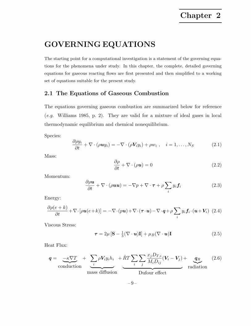
2.1 The Equations of Gaseous Combustion

The equations governing gaseous combustion are summarized below for reference

(e.g. Williams 1985, p. 2). They are valid for a mixture of ideal gases in local

thermodynamic equilibrium and chemical nonequilibrium.

Species:∂ρyi∂t

+∇ · (ρuyi) = −∇ · (ρViyi) + ρwi , i = 1, . . . , NS (2.1)

Mass:∂ρ

∂t+∇ · (ρu) = 0 (2.2)

Momentum:∂ρu

∂t+∇ · (ρuu) = −∇p+∇ · τ + ρ

∑

i

yifi (2.3)

Energy:

∂ρ(e+ k)

∂t+∇· [ρu(e+k)] = −∇·(pu)+∇·(τ ·u)−∇·q+ρ

∑

i

yifi ·(u+Vi) (2.4)

Viscous Stress:

τ = 2µ [S− 13(∇ · u)I] + µB(∇ · u)I (2.5)

Heat Flux:

q = −κ∇T︸ ︷︷ ︸conduction

+∑

i

ρViyihi

︸ ︷︷ ︸mass diffusion

+ RT∑

i

∑

j

xjDT,i

MiDij(Vi − Vj)

︸ ︷︷ ︸Dufour effect

+ qR︸︷︷︸radiation

(2.6)

– 9 –

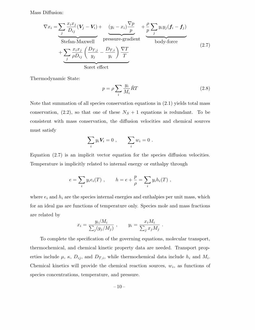
Mass Diffusion:

∇xi =∑

j

xixjDij

(Vj − Vi)

︸ ︷︷ ︸Stefan-Maxwell

+ (yi − xi)∇pp︸ ︷︷ ︸

pressure-gradient

+ρ

p

∑

j

yiyj(fi − fj)

︸ ︷︷ ︸body-force

+∑

j

xixjρDij

(DT,j

yj− DT,i

yi

) ∇TT

︸ ︷︷ ︸Soret effect

(2.7)

Thermodynamic State:

p = ρ∑

i

yiMi

RT (2.8)

Note that summation of all species conservation equations in (2.1) yields total mass

conservation, (2.2), so that one of these NS + 1 equations is redundant. To be

consistent with mass conservation, the diffusion velocities and chemical sources

must satisfy∑

i

yiVi = 0 ,∑

i

wi = 0 .

Equation (2.7) is an implicit vector equation for the species diffusion velocities.

Temperature is implicitly related to internal energy or enthalpy through

e =∑

i

yiei(T ) , h = e+p

ρ=∑

i

yihi(T ) ,

where ei and hi are the species internal energies and enthalpies per unit mass, which

for an ideal gas are functions of temperature only. Species mole and mass fractions

are related by

xi =yi/Mi∑j(yj/Mj)

, yi =xiMi∑j xjMj

.

To complete the specification of the governing equations, molecular transport,

thermochemical, and chemical kinetic property data are needed. Transport prop-

erties include µ, κ, Dij , and DT,i, while thermochemical data include hi and Mi.

Chemical kinetics will provide the chemical reaction sources, wi, as functions of

species concentrations, temperature, and pressure.

– 10 –

2.2 Simplifying Assumptions

For the large-scale simulations undertaken in this study, it is necessary to simplify

the governing equations of §2.1, although when computations of flamelet solutions

are considered in §3.3 it will be found that many of the simplifications are unnec-

essary. We adopt a standard set of assumptions that are well justified for many

combustion systems and have been used in many previous studies. Accordingly, the

following phenomena are neglected in this study:

• acoustic interactions and compressibility

• heating due to viscous dissipation

• bulk viscosity

• body forces

• diffusion due to pressure gradients

• thermal radiation

Furthermore, it will be convenient to express mass-diffusion processes in Fick’s Law

form by assigning a mixture diffusivity, αi, to each species. The species diffusion

velocities are then given by

Vi = −αi∇yiyi

. (2.9)

A simple formula for calculating approximate mixture diffusivities from the binary

diffusivity matrix (Bird et al. 1960, p. 571) is,

αi =1− xi∑

j 6=i

xjDij

. (2.10)

A problem can arise when using (2.9) in that the resulting diffusion velocities do

not necessarily satisfy∑

i yiVi = 0. A simple remedy is to subtract any residual

“Stefan flow” from the bulk flow velocity in the species transport equations,

∇ · (ρuyi) −→ ∇ · [ρ(u−∑jyjVj)yi] ,

thereby cancelling any bulk flow arising from the diffusional mass fluxes.

– 11 –

The separate assumptions that acoustics and viscous heating are negligible

are often lumped together into what is commonly called the “low Mach number

approximation”, though depending on the application, either of these phenomena

could still be important even if the flow nominally has a very low Mach number.

While these assumptions stipulate that the flow be low Mach number, the converse

is not necessarily true.

In neglecting acoustic interactions and compressibility, it is assumed that ther-

modynamic variables such as density, temperature, enthalpy, and entropy are de-

coupled from variations in pressure, δp, about some specified background pressure

field, p0. This would mean, for example, that

ρ(p0 + δp, s) ' ρ(p0, s) , or

(∂ρ

∂p

)

s

' 0 ,

which, of course, implies that the speed of sound is nearly infinite. With this

approximation, only p0 is coupled to the thermodynamic variables and enters into

the equation of state,

p0 = ρ∑

i

yiMi

RT . (2.11)

For the open systems considered in this study it is also assumed that p0 is uniform

and constant so that the material derivative of pressure in the enthalpy equation

reduces to

Dp

Dt' Dp0

Dt= 0 .

In addition to the above approximations, the “unity Lewis numbers” assump-

tion (equal diffusivities for all species and temperature) is used for large-scale trans-

port, where turbulent advection dominates. However, differential diffusion effects

can still be important at the small scales, and in such cases, differential diffusion

can be included in subgrid-scale models for turbulent combustion but can generally

be ignored when solving the transport equations for the large scales.

The above assumptions are now used to derive simplified forms of the energy

equation for reacting flows, starting with the internal energy equation (obtained by

– 12 –

subtracting kinetic energy from total energy) in enthalpy form:

∂ρh

∂t+∇ · (ρuh) = Dp

Dt+ τ : ∇u−∇ · q + ρ

∑

i

yifi · Vi . (2.12)

After neglecting acoustic interactions, viscous dissipation, and body forces, this

simplifies to:∂ρh

∂t+∇ · (ρuh) = Dp0

Dt−∇ · q . (2.13)

Then, assuming constant p0, rewriting the left-hand side in advective form, and

substituting for the heat flux vector while neglecting radiation and the Dufour

effect, one obtains:

ρDh

Dt= ∇ · (κ∇T −

∑

i

ρViyihi) . (2.14)

To generate more useful forms, the following identity is helpful:

∇h = ∇∑

i

yihi =∑

i

yi∇hi +∑

i

hi∇yi

=∑

i

yicp,i∇T +∑

i

hi∇yi

= cp∇T +∑

i

hi∇yi .

(2.15)

Using this relation and the species conservation equations, the left-hand-size of

(2.14) may be expressed as:

ρDh

Dt= ρcp

DT

Dt+∑

i

hi ρDyiDt

= ρcpDT

Dt+∑

i

hi [−∇ · (ρViyi) + ρwi] .

Substituting this into (2.14) and rearranging yields:

ρcpDT

Dt= ∇ · (κ∇T )−

∑

i

ρcp,i yiVi · ∇T −∑

i

ρhiwi . (2.16)

This is the standard form of the energy equation for reacting flows when temperature

is used as a primitive variable. It should be noted that under assumption of equal

specific heats for all species, the mass diffusion term in (2.16) is zero.

To avoid the reaction source term in (2.16), it is often desirable to work with

total enthalpy. Returning to (2.14) and substituting Fick’s Law for the diffusion

velocities, we have,

ρDh

Dt= ∇ · (κ∇T +

∑

i

ραihi∇yi) . (2.17)

– 13 –

Using the identity (2.15) to eliminate ∇T , the following form can be derived:

ρDh

Dt= ∇ · (ραT∇h) +∇ · [

∑

i

ρ(αi − αT )hi∇yi] . (2.18)

Under the assumption of unity Lewis numbers, αi = αT , this reduces to

ρDh

Dt= ∇ · (ραT∇h) . (2.19)

With this last step, the energy equation has been written as a simple advection-

diffusion equation for a conserved scalar. If, in addition, adiabatic walls are as-

sumed, then enthalpy and mixture fraction (§3.3.1) have the same boundary condi-

tions and are linearly dependent.

2.3 Working Equation Set

With the assumptions and simplifications of §2.2, the governing equations used for

this study may be written as follows:

Continuity:∂ρ

∂t+∇ · (ρu) = 0 (2.20)

Momentum:

∂ρu

∂t+∇ · (ρuu) = −∇p+∇ ·

[2µ(S− 1

3I∇ · u)

](2.21)

Scalar Transport:

∂ρφk∂t

+∇ · (ρuφk) = ∇ · (ραk∇φk) + ρwk , k = 1, 2, . . . (2.22)

State Relation:

ρ = f(φ1, φ2, . . .) (2.23)

Note that the equation of state (2.23) has been reduced from (2.11) to an expression

for density in terms of the transported scalars. In general, the set of transported

scalars carried in a simulation, φk, could include mixture fraction, total enthalpy, a

particular chemical species, or some more complicated composite quantity. In this

– 14 –

work, however, the only scalar equations considered are for mixture fraction and a

progress variable.

Chemical property data, which are needed to determine ρ, µ, αk, and wk in

terms of the φk, are provided by the chemistry models discussed in §3.3. The

chemistry model will also provide complete chemical state information — data for

all chemical species and temperature — in terms of the φk, even though only a

small number of scalars are carried in (2.22).

– 15 –

– 16 –

Chapter 3

TURBULENCE ANDCHEMISTRY MODELS

In this work, solutions to the reacting flow equations are obtained using the technique of

large eddy simulation. The large, energy-containing scales of motion are simulated nu-

merically while the small, unresolved scales and their interactions with the large scales are

modeled. In this chapter, large eddy simulation principles are first reviewed; then standard

dynamic models for subgrid stress, scalar flux, and scalar variance are given, and the as-

sumed beta pdf for subgrid fluctuations of a conserved scalar is discussed. The chemistry

models used in this work are all based on mixture fraction, which plays a fundamental role

in non-premixed combustion. Traditional mixture-fraction based modeling approaches are

discussed, and a new flamelet approach incorporating a progress variable is presented.

3.1 Filtering and the LES Equations

In large eddy simulation (les), all of the field variables are decomposed into re-

solved and subgrid-scale parts. The resolved, large-scale fields are related to the

instantaneous full-scale fields through a grid-filtering operation (indicated by an

overbar symbol) that removes scales too small to be resolved by the simulation.

Note that in the present study, filtering is implicitly defined by the computational

grid used for the large-scale equations and that explicit filtering (Ghosal and Moin

1995; Vasilyev et al. 1998) is not used. Quantities per unit volume are treated using

a Reynolds decomposition,

ρ = ρ+ ρ′ ,

while quantities per unit mass are best described by a Favre (density-weighted)

decomposition,

u = u+ u′′ ,

where

u = ρu / ρ .

– 17 –

Note that with the Favre decomposition, filtered variables represent “mixed-mean”

averages over subgrid volumes. This ensures that the filtering process does not alter

the form of the conservation laws.

The les equations for the resolved fields are formally derived by substituting

the above decompositions into the governing equations, and then subjecting the

equations to the grid filter. The instantaneous small-scale fluctuations are removed

by the filter, but their statistical effects remain in unclosed residual terms repre-

senting the influence of the subgrid scales on the resolved scales. Applying this

procedure to the working equations of §2.3, the les equations are written (now

using subscript notation) as:

Continuity:

ρ,t + (ρuj),j = 0 (3.1)

Momentum:

(ρui),t + (ρuiuj),j = −p,i + (2µSij),j + tij,j (3.2)

Sij =12(ui,j + uj,i)− 1

3δij uk,k

Scalar Transport:

(ρφi),t + (ρuj φi),j = (ραiφi,k),k + ρwi + qik,k (3.3)

State Relation:

ρ = f(φ1, φ2, . . .) (3.4)

All unclosed transport terms in the momentum and scalar equations are grouped

into the residual stress, tij , and residual scalar flux, qik. These terms as well as the

filtered chemical source terms, wi, and the state relation require closure modeling.

3.2 Subgrid-Scale Models

Subgrid closure models for (3.1–3.4) are presented below. The dynamic procedure is

first summarized in §3.2.1 because it is used whenever applicable to evaluate model

coefficients. Closures for the filtered chemical source terms and the state relation,

which are related to the chemical model, are discussed in §3.3.

– 18 –

3.2.1 The Dynamic Procedure

Since many of the subgrid closures considered utilize the dynamic modeling concept

(Germano et al. 1991), it is briefly reviewed here in general form. The dynamic

procedure is a method for calculating dimensionless scaling coefficients in subgrid-

scale models for filtered nonlinear terms.

Consider an arbitrary nonlinear term, t(u), which is a known function of the

field variables, u, and suppose that we wish to determine its filtered value by model-

ing the subgrid residual with an algebraic model, m(u), which depends on the field

variables but in general can also depend explicitly on space and time and on other

parameters such as the grid filter width, ∆. The value of the filtered term is then

the sum of resolved and modeled parts:

t(u) = t(u) +m(u) . (3.5)

The basic idea behind the dynamic procedure is to consider how t(u) and m(u) vary

with the filter width. In particular, an expression similar to (3.5) for the value of

the filtered term at a larger filter width, referred to as the test filter, can be written:

t(u) = t(u) +m(u) . (3.6)

In dynamic modeling, filtering to the test level is indicated by a hat symbol. The

test filter width is denoted by ∆ and is usually taken to be twice the width of the

grid filter, ∆ = 2∆.

If (3.5) is test filtered and subtracted from (3.6), an interesting identity results:

t(u)− t(u) = m(u)− m(u) . (3.7)

Remarkably, all terms in this equation are computable from the known resolved

field. It represents the “band-pass filtered” contribution to the nonlinear term in

the scale range between the grid and test filter levels. A consistent subgrid model

should contribute the same amount as the resolved field in this band. The key

to the dynamic procedure is to use this identity as a constraint for calibration of

subgrid-scale models.

– 19 –

Note that while (3.7) is an exact identity when m(u) is the exact subgrid

residual, it should only be expected to hold in a statistical sense (and should not

be applied locally and instantaneously) when m(u) is modeled. The reason for

this is the following: In filtering the governing equations, we have replaced the

instantaneous variations that occur within each subgrid volume with a statistical

description of the subgrid state. However, the band-pass filtered fields in (3.7) are

based on instantaneous data, and the test filtering process itself does not provide

sufficient averaging to produce converged statistics in the band-pass filtered scale

range. Furthermore, subgrid models are generally valid for predicting statistical

properties of the subgrid scales but usually cannot account for instantaneous subgrid

fluctuations. Requiring (3.7) to be satisfied locally forces the model to operate

beyond its range of validity, resulting in unphysical fluctuations in model behavior.

This may explain why les practitioners have found that some form of averaging is

required in order to compute stable model coefficients with the dynamic procedure.

Related discussions are given by Ghosal et al. (1995) and Carati and Eijnden (1997).

For the dynamic procedure to be applicable, the quantity to be modeled must

vary substantially between the grid and test filter scales; otherwise, the difference in

(3.7) will not be significant and cannot be used for modeling subgrid-scale quantities.

Examples of quantities that cannot be modeled dynamically are dissipation and

chemical reaction rates, because these phenomena occur almost exclusively at the

smallest scales, which are always unresolved in les.

The dynamic procedure is usually applied to situations in which the subgrid

model can be written as,

m(u) = c s(u,∆) , (3.8)

where s(u,∆) is a dimensionally consistent algebraic scaling law and c is an unknown

dimensionless coefficient, which in the dynamic procedure is allowed to vary in space

and time. Substituting this form into (3.7) we obtain,

t(u)− t(u) = c∗s(u, ∆)− c s(u,∆) , (3.9)

where c∗ is the model coefficient at the test filter level. Note that c has been left

– 20 –

inside the test filtering operator in the right most term.

At this point, the various forms of the dynamic procedure differ as to how

to use this equation to calculate the model coefficient, c. In the present study,

it is assumed that c is a statistical quantity that varies slowly in space and time

and is both scale invariant and independent of the directions in which the flow is

statistically homogeneous. We therefore set c∗ = c and allow c to pass through the

test filtering operator. To simplify notation the following substitutions are made:

L = t(u)− t(u) , M = s(u, ∆)− s(u,∆) ,

where, L is called the Leonard term and M is the model term. The equation for c

can then be written as,

L = cM . (3.10)

To obtain a single value for c in each homogeneous region of the flow, and to

determine c in cases where L and M are nonparallel vectors or tensors, (3.10) is

solved by least-squares (Lilly 1992). The final expression is:

c =〈L ·M〉〈M ·M〉 , (3.11)

where the angle brackets indicate averaging over directions of flow homogeneity.

3.2.2 Turbulent Stress and Scalar Flux

Subgrid momentum and scalar transport terms that appear in (3.2) and (3.3) are

modeled using the dynamic approach of Moin et al. (1991). The present formulation

differs from Moin et al. in the use of the deviatoric strain rate for the definition of

|S| and in the use of least-squares averaging.

The residual stresses are modeled as subgrid turbulent stresses with an eddy

viscosity assumption,

tij = −ρuiuj + ρ uiuj = 2µtSij − 13ρq2δij , (3.12)

where 12ρq2 is the subgrid kinetic energy and,

Sij =12(ui,j + uj,i)− 1

3δij uk,k .

– 21 –

The eddy viscosity is given by the Smagorinsky model,

µt = Cµρ∆2|S| , where |S| =

√SijSij , (3.13)

and the subgrid kinetic energy is modeled using,

ρq2 = Ckρ∆2|S|2 . (3.14)

Note, however, that the isotropic part of the residual stress does not need to be mod-

eled separately when pressure is decoupled from thermodynamic variables, because

it may then be lumped together with the pressure. In the present study, acoustic

interactions and compressibility are neglected, so in the interest of computational

efficiency, this term is not actually computed.

The residual scalar fluxes are modeled as subgrid turbulent scalar fluxes with

a gradient-diffusion assumption,

qik = −ρukφi + ρ ukφi = ραtφi,k , (3.15)

where the eddy diffusivity is given by,

ραt = Cαρ∆2|S| . (3.16)

Note that the eddy diffusivity model has the same algebraic form as the eddy vis-

cosity model, but the model coefficient is different. The ratio of the two coefficients

gives the subgrid turbulent Prandtl number, Prt = Cµ/Cα.

The coefficients in all of these models, Cµ, Ck, and Cα, are evaluated using the

dynamic procedure. To simplify the expressions for the coefficients, the following

notation for density-weighted test filtering is introduced:

ˇu = ρ u / ρ .

For the subgrid turbulent stress model (3.12) the dynamic procedure gives,

Cµ =〈LijMij〉

2 〈MklMkl〉, Lij = −ρ uiuj + ρ uiuj , Mij = ρ∆2| ˇS| ˇSij − ρ∆2|S|Sij .

– 22 –

For the subgrid turbulent scalar flux model (3.15) the coefficient is calculated from,

Cα =〈LiMi〉〈MjMj〉

, Li = −ρuiφ+ ρˇuiˇφ , Mi = ρ∆2| ˇS|ˇφ,i − ρ∆2|S|φ,i .

Although it is not actually used in the present study, the expression for the subgrid

kinetic energy coefficient is the following:

Ck =〈LM〉〈M2〉 , L = ρ ukuk − ρ ˇuk ˇuk , M = ρ∆2| ˇS|2 − ρ∆2|S|2 .

There is a minor defect in the dynamic procedure when applied to scalar trans-

port: In a region where the flow is turbulent but the scalar is uniform or fully

mixed, the dynamic procedure does not define an eddy diffusivity. When this sit-

uation arises in practice, the eddy diffusivity is set to zero. This normally does

not pose a problem in regions of uniform scalar because the scalar gradient, which

multiplies the eddy diffusivity, is also zero. However, since scalar transport is linear

in the scalar, the eddy diffusivity should in principle depend only on the velocity

field, should be the same for all scalars, and should be nonzero where the velocity is

turbulent. When multiple scalar transport equations are solved simultaneously, one

could compute a different eddy diffusivity for each scalar, or compute a least-squares

average diffusivity using all the scalars, or base the eddy diffusivity calculation on

a single, chosen scalar. In the present study, eddy diffusivity is computed using the

mixture fraction and then applied to all scalars.

3.2.3 Variance and Dissipation Rate of a Conserved Scalar

Subgrid scalar variance is an input parameter to the assumed pdf model of §3.2.4,while scalar dissipation rate is a parameter in flamelet models of turbulent combus-

tion (§3.3.3). Starting from assumptions of local homogeneity and local equilibrium

for the subgrid scales, Pierce and Moin (1998c) derived algebraic models for subgrid

variance and dissipation rate. The subgrid variance is modeled using,

ρ φ′′2 = Cφ ρ∆2|∇φ|2 , (3.17)

– 23 –

and the filtered dissipation rate, ρ χ = ραm|∇φ|2, is modeled by,

ρ χ = ρ(αm + αt)|∇φ|2 , (3.18)

where αm is the molecular diffusivity and αt is the turbulent diffusivity of §3.2.2.Dynamic evaluation of Cφ is summarized by the following:

Cφ =〈LM〉〈M2〉 , L = ρ φφ− ρ ˇφˇφ , M = ρ∆2|∇ˇ

φ|2 − ρ∆2|∇φ|2 .

Pierce and Moin presented (3.17) as an alternative to the scale-similarity model

of Cook and Riley (1994). An alternative derivation for (3.18) to that of Girimaji

and Zhou (1996) was presented to emphasize the local equilibrium and dynamic

modeling ideas. Note that when (3.17) is applied to mixture fraction, the dynamic

procedure does not guarantee that the predicted variance is physically realizable. In

practice, variance predictions lying outside the physically allowed range, 0 ≤ Z ′′2 ≤Z(1− Z), are clipped.

3.2.4 Assumed Beta PDF for a Conserved Scalar

While algebraic scaling laws and scale-similarity concepts can be expected to work

for quadratic nonlinearities, the only acceptable closure for arbitrary nonlineari-

ties appears to be the probability density function (pdf) approach. For example,

the state relation for density (3.4) can in general be an arbitrary nonlinear func-

tion of the scalar variables. If the joint pdf of the subgrid scalar fluctuations,

P (φ1, φ2, . . .), were known, the filtered density could be evaluated using,

ρ = f(φ1, φ2, . . .) =

∫f(φ1, φ2, . . .)P (φ1, φ2, . . .) dφ1 dφ2 . . . . (3.19)

When Favre filtering is used for the scalar variables, it is more appropriate to eval-

uate filtered quantities using the joint Favre pdf of the subgrid scalar fluctuations.

Analogous to (3.19), Favre-filtered quantities would be evaluated using,

y =

∫y(φ1, φ2, . . .)P (φ1, φ2, . . .) dφ1 dφ2 . . . , (3.20)

– 24 –

where the density-weighted Favre pdf is related to the standard pdf by,

P (φ1, φ2, . . .) =ρ(φ1, φ2, . . .)P (φ1, φ2, . . .)

ρ. (3.21)

The Reynolds-filtered density can be obtained using P by dividing (3.21) by ρ and

integrating, with the result that,

ρ =

[∫P (φ1, φ2, . . .)

ρ(φ1, φ2, . . .)dφ1 dφ2 . . .

]−1. (3.22)

In the assumed pdf method, the probability density function is modeled di-

rectly using simple analytical forms, such as the beta distribution. However, because

source terms can directly modify the pdf of a scalar, the beta distribution can be

expected to be valid only for conserved scalars. For this reason, it is applied only to

mixture fraction in this work. Assumed-pdf modeling of reacting scalars is a topic

for further research.

The two-parameter family of beta distributions on the interval, 0 ≤ x ≤ 1, is

given by,

P (x; a, b) = xa−1(1− x)b−1 Γ(a+ b)

Γ(a) Γ(b), (3.23)

where the parameters a and b are related to the distribution mean and variance

(µ, σ2) by

a =µ(µ− µ2 − σ2)

σ2, b =

(1− µ)(µ− µ2 − σ2)σ2

.

When applied to mixture fraction, x→ Z, µ→ Z, and σ2 → Z ′′2.

The beta pdf has been evaluated as a model for subgrid mixture fraction

fluctuations in large eddy simulations in several studies using a priori tests on

direct numerical simulation data. Cook and Riley (1994) tested the beta pdf in the

context of the fast chemistry model (§3.3.2) in homogeneous turbulence. Jimenez

et al. (1997) demonstrated the good performance of the beta pdf model using data

from a highly intermittent, incompressible, turbulent mixing layer. Wall and Moin

(2000) tested the beta pdf in the presence of heat release. It has also been shown

(Wall et al. 2000; Cook and Riley 1994) that accurate prediction of the subgrid

variance is the most important factor in obtaining good results with the beta pdf.

– 25 –

The state relation and other nonlinear functions are often known prior to con-

ducting a simulation, in which case the pdf integrals can be calculated and stored

into lookup tables before the simulation begins. The filtered density and other fil-

tered quantities can then be efficiently retrieved during the simulation as functions

of the known filtered scalars and variances:

ρ = F (φ1, φ2, . . . , φ′′21 , φ′′22 , φ

′′1φ

′′2 , . . .) . (3.24)

3.3 Chemistry Models

Developing effective strategies for incorporating chemistry into large eddy simula-

tions was one of the main objectives of this work. The straightforward, brute-force

approach would be to find a suitable chemical kinetic mechanism for the system

under investigation, solve scalar transport equations for all the species in the mech-

anism, and attempt to model the filtered source term in each equation.

A serious problem with this direct approach is that realistic kinetic mechanisms

can involve tens of species and hundreds of reaction steps, even for “simple” fuels

such as methane. Unless mechanism reduction methodologies can drastically reduce

the dimensionality of the chemical system, one is faced with having to solve a large

number of stiffly coupled scalar transport equations.

Another problem is that each species transport equation contains a filtered

chemical source term that must be modeled. Like the state relation (3.4), each

chemical source term is, in principle, an arbitrary nonlinear function of the scalar

variables. As discussed in §3.2.4, pdf methods are the most attractive approach for

evaluating such nonlinearities; however, when the number of independent variables

becomes large (say, more than three) joint pdf’s can become unwieldy.

Thus, the key to combustion modeling in les appears to be minimizing the

number of transported scalar variables required. For non-premixed combustion,

mixture-fraction based models appear to offer the most effective description of the

chemistry. By mapping the details of the multicomponent diffusion-reaction pro-

cesses to a small number of “tracking” scalars, complete chemical state information

can be obtained at greatly reduced computational expense.

– 26 –

3.3.1 The Role of Mixture Fraction

All of the chemistry models considered in this work are based on the concept of

mixture fraction. The role of mixture fraction in non-premixed combustion is best

described as a tracking scalar because it tracks the mixing of inflow streams, the

transport of conserved scalars, and the advection of reactive scalars.

A Mixture Tracking Scalar

At its most basic level, mixture fraction (denoted by Z in this work) is a generic

mixing variable that represents the relative amount that each inflow stream con-

tributes to the local mixture. When the the inflow streams are fuel and oxidizer,

mixture fraction can be thought of as specifying the fuel-air ratio or stoichiometry

of the local mixture.

Mixture fraction is also a conserved scalar that is representative of other con-

served scalars in the flow. Equations for conserved scalars can be formally derived

by taking linear combinations of species transport equations in such a way that

reaction source terms cancel. The resulting equation will describe a physical quan-

tity that is conserved during chemical reaction, such as total enthalpy or the mass

fraction of a particular chemical element. Except for differences due to effects of

differential diffusion and boundary conditions, every conserved scalar satisfies the

advection-diffusion equation, here written for mixture fraction:

∂ρZ

∂t+∇ · (ρuZ) = ∇ · (ραZ∇Z) . (3.25)

Because conserved scalar transport is linear, a small number of conserved scalars

forming a complete basis is sufficient to construct all other conserved scalars by

superposition. A flow system containing n inflow ports would in general require n

mixture fraction variables to form a complete basis, but because all the normalized

mixture fractions must sum to unity, only n − 1 mixture fraction variables are

needed. By convention, a mixture fraction variable is assigned the value 1 in the

flow port from which it emanates and zero in all others. Values of mixture fraction

between 0 and 1 indicate the mass fraction that a particular stream contributes to

the local mixture.

– 27 –

The standard mixture fraction used in non-premixed combustion, Z, is the fuel-

stream mixture fraction and is therefore unity in the fuel stream and zero in the

oxidizer stream. The mixture fraction for the oxidizer stream is then given by 1−Z.When there are more than two inflow ports supplying independent species composi-

tions and/or enthalpy content, an additional mixture fraction variable can be added

for each additional port. When thermal radiation or heat transfer to boundaries

is important, total enthalpy should be treated as an independent conserved scalar,

but otherwise it can be directly related to mixture fraction.

Utility with Differential Diffusion

In the absence of differential diffusion, the diffusivity in (3.25) is the same for all

scalars and mixture fraction tracks other conserved scalars exactly. However, when

differential diffusion effects are present, mixture fraction tracks other conserved

scalars only approximately. As noted in §2.2, differential diffusion can generally be

neglected in the large scale transport resolved by les, and therefore, considerations

of differential diffusion will be limited mainly to the subgrid-scale model.

With differential diffusion, the mixture fraction concept is still very useful, but

the definition of mixture fraction is not as straightforward. Pitsch and Peters (1998)

suggest that (3.25), with αZ prescribed, be taken as the definition of Z. But in the

present work, an average mixture fraction is defined by combining the conserved

elemental (atomic) mass fractions. The elemental mass fractions, aj , are given in

terms of the species mass fractions by,

aj =∑

i

yiNijAj/Mi , j = 1, . . . , NE , (3.26)

where Nij is the number of j atoms in each molecule of species i, Aj are atomic

weights, and NE is the total number of distinct chemical elements present in the sys-

tem. The average mixture fraction for a two-feed system is then given by summing

the elemental mass fractions and normalizing the result,

Z =

∑i |ai − a0i |∑j |a1j − a0j |

, (3.27)

– 28 –

where a0i and a1i are elemental mass fractions in the oxidizer and fuel streams,

respectively. Also, an average mixture-fraction diffusivity can be defined in a similar

manner by combining the elemental diffusive fluxes,

aj =∑

i

ρyiViNijAj/Mi , j = 1, . . . , NE , (3.28)

and equating the mixture fraction flux to the normalized result,

ραZ |∇Z| =∑

i |ai|∑j |a1j − a0j |

. (3.29)

Note that (3.27) and (3.29) are consistent with each other such that solving (3.25)

with αZ given by (3.29) is equivalent to using (3.27). The above definitions are used

in the present work to define mixture fraction and its diffusivity when computing

flamelet solutions in physical space (§3.3.3).

Utility in Flamelet Models

Another important property of the mixture fraction is its ability to account for tur-

bulent advection in diffusion flames. Because the velocity field transports all scalars

equally, changes in species mass fractions with respect to mixture fraction are due

only to diffusion and reaction. (In the absence of diffusion and reaction, relation-

ships between mixture fraction and other scalars would be exactly preserved.) The

implication is that turbulent combustion, when viewed relative to mixture fraction,

is simply laminar diffusion-reaction in an unsteady straining environment created by

turbulent advection. This principle is the basis of flamelet models, in which explicit

velocity dependence is removed from the scalar transport equations by relating the

scalars to the mixture fraction, which itself does depend on the velocity field.

By itself, mixture fraction does not contain any information about chemical

reactions in the mixture. Assumptions such as fast chemistry or steady flamelet

state relationships are needed to associate a chemical state with the mixture frac-

tion. Also, mixture fraction cannot account for chemical variations in directions

perpendicular to its gradient. To address these and other problems, an additional

tracking scalar in the form of a progress variable is introduced in §3.3.4.

– 29 –

3.3.2 Fast Chemistry Assumption

One of the simplest approaches for relating chemical states to mixture fraction is

to assume equilibrium chemistry , the condition that chemical kinetics are infinitely

fast relative to other processes in the flow (high Damkohler number limit), so that

the mixture is always completely reacted, or in a state of chemical equilibrium.

A similar assumption, called fast chemistry (also known as the Burke-Schumann

limit), is equilibrium chemistry combined with a one-step, global reaction or “major

products” assumption. The opposite extreme of fast chemistry is the case of pure

mixing (or frozen chemistry), the limit in which chemical reactions are negligible.

With each of these assumptions the chemical composition is a unique function

of mixture stoichiometry, total enthalpy, and pressure. For constant background

pressure, unity Lewis numbers, negligible thermal radiation, and adiabatic walls,

all chemical variables become functions of mixture fraction alone:

yi = yi(Z) , T = T (Z) , ρ = ρ(Z) . (3.30)

These functions constitute what may be called “chemical state relationships”, and

can be computed using an equilibrium chemistry code such as stanjan (Reynolds

1986). When combined with the assumed pdf of §3.2.4 for mixture fraction, this

provides complete closure for the problem, and all of the filtered combustion vari-

ables can be expressed as functions of filtered mixture fraction and mixture fraction

variance:

yi = yi(Z, Z ′′2) , T = T (Z, Z ′′2) , ρ = ρ(Z, Z ′′2) , etc. (3.31)

Note that (3.31) includes similar expressions for filtered transport properties such

as µ and αZ , which are used when solving the large-scale momentum and scalar

transport equations. The computational cost of the fast chemistry model is negli-

gible, because the functions in (3.31) can be precomputed and tabulated prior to

running a simulation.

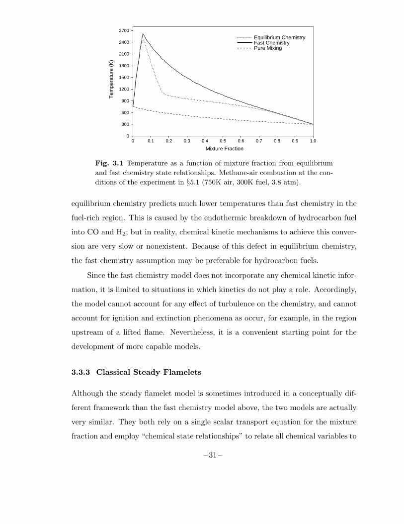
Example state relationships for temperature, T (Z), are plotted in Fig. 3.1 for

equilibrium chemistry, fast chemistry, and pure mixing assumptions. Note that

– 30 –

Mixture Fraction

Tem

pera

ture

(K

)

0 0.1 0.2 0.3 0.4 0.5 0.6 0.7 0.8 0.9 1.00

300

600

900

1200

1500

1800

2100

2400

2700

Equilibrium ChemistryFast ChemistryPure Mixing

Fig. 3.1 Temperature as a function of mixture fraction from equilibrium

and fast chemistry state relationships. Methane-air combustion at the con-

ditions of the experiment in §5.1 (750K air, 300K fuel, 3.8 atm).

equilibrium chemistry predicts much lower temperatures than fast chemistry in the

fuel-rich region. This is caused by the endothermic breakdown of hydrocarbon fuel

into CO and H2; but in reality, chemical kinetic mechanisms to achieve this conver-

sion are very slow or nonexistent. Because of this defect in equilibrium chemistry,

the fast chemistry assumption may be preferable for hydrocarbon fuels.

Since the fast chemistry model does not incorporate any chemical kinetic infor-

mation, it is limited to situations in which kinetics do not play a role. Accordingly,

the model cannot account for any effect of turbulence on the chemistry, and cannot

account for ignition and extinction phenomena as occur, for example, in the region

upstream of a lifted flame. Nevertheless, it is a convenient starting point for the

development of more capable models.

3.3.3 Classical Steady Flamelets

Although the steady flamelet model is sometimes introduced in a conceptually dif-

ferent framework than the fast chemistry model above, the two models are actually

very similar. They both rely on a single scalar transport equation for the mixture

fraction and employ “chemical state relationships” to relate all chemical variables to

– 31 –

the mixture fraction. The only difference is that the steady flamelet model replaces

equilibrium chemical states (obtained from thermochemistry alone) with solutions

to one-dimensional, steady, diffusion-reaction equations. The chemical reactions,

although finite-rate, are assumed to be at all times in balance with the rate at

which reactants diffuse into the flame, so that flame properties are directly related

to the scalar dissipation (or mixing) rate. The result is a modest improvement over

fast chemistry, allowing for more realistic chemical state relationships. Like the fast

chemistry model, steady flamelets cannot account for extinction (when reaction rate

is lower than mixing rate), ignition (when reaction rate is higher than mixing rate),

or the effects of unsteady mixing (when reaction rate lags behind changes in mixing

rate). The flamelet/progress-variable approach discussed in §3.3.4 overcomes all of

these limitations by using a (dynamic) chemical variable instead of the (kinematic)

dissipation rate to parameterize flamelet evolution.

One approach to deriving the steady flamelet model is to start with the as-

sumption that in each region of the flow, all chemical species are given by unique

functions of the mixture fraction,

yi = fi(Z) . (3.32)

Derivatives of chemical species can then be related to derivatives of mixture fraction:

yi,t = f ′iZ,t , yi,j = f ′iZ,j . (3.33)

For (3.32) to be valid locally, species mass fractions must vary slowly in directions

perpendicular to the mixture-fraction gradient and chemical reactions must be in

balance with species diffusion along the mixture-fraction gradient, so that the flame

is locally one-dimensional and steady.

Using (3.33), the species conservation equations can be “transformed” from

physical space to mixture-fraction space. For the moment, assume unity Lewis

numbers so that all species, enthalpy, and mixture fraction have a common diffusiv-

ity, α. Substituting (3.33) into the species transport equations (2.1) and rearranging

while noting that f ′i,k = f ′′i Z,k, one obtains,

f ′i [ρ(Z,t + uj Z,j)− (ραZ,k),k] = ραZ,kZ,kf′′i + ρwi .

– 32 –

The quantity in brackets on the left-hand side of this equation is identically zero,

leaving us with the steady flamelet equations,

ρχd2yidZ2

= −ρwi , (3.34)

where χ = αZ,kZ,k is the mixture-fraction dissipation rate. In order to solve (3.34),

an additional assumption is needed to prescribe the dissipation rate as a function

of mixture fraction, χ = χ(Z).

Physical-Space Formulation

In the present study, the flamelet equations are formulated and solved in physi-

cal space rather than in mixture-fraction space, and the physical-space solutions

are later remapped to mixture fraction. In physical space, it is more natural to

consider the full combustion equations of §2.1 and reduce them to the case of one-

dimensional, steady combustion. Most of the assumptions of §2.2 are maintained,

except that the full multicomponent diffusion mechanisms (including Soret and

Dufour effects) may be used. Continuity and momentum equations are not solved

because the velocity is to be imposed. The physical space (x-coordinate) flamelet

equations can then be written as:

ρuyi,x = −(ρyiVi),x + ρwi ,

ρuh,x = (κT,x −∑

iρViyihi − qD),x ,

h =∑

iyihi(T ) ,

ρ = p0/∑

i

yiMi

RT ,

(3.35)

where qD is the Dufour heat flux. Mixture fraction is defined in terms of the species

mass fractions by (3.27), but one could instead include an equation for mixture

fraction,

ρuZ,x = (ραZZ,x),x , (3.36)

in which αZ would be prescribed. Note that solving (3.36) with αZ given by (3.29)

is equivalent to using (3.27).

– 33 –

x / L

Te

mp

era

ture

(K

)

0 0.2 0.4 0.6 0.8 1.00

300

600

900

1200

1500

1800

2100

2400

x / L

Mix

ture

Fra

ctio

n

0 0.2 0.4 0.6 0.8 1.0

0

0.2

0.4

0.6

0.8

1.0

Fig. 3.2 Mixture fraction and temperature from a steady flamelet solu-

tion in physical space. Methane-air combustion at the conditions of the

experiment in §5.1 (750K air, 300K fuel, 3.8 atm). L = 0.2 cm.

Like the dissipation rate in (3.34), the velocity in the physical-space equations,

u(x), needs to be prescribed. In fact, the solution of (3.36) with an assumed form

for u(x) yields a corresponding χ(Z). The standard flamelet approach (Peters 1984;

Cook et al. 1997) usually assumes a counterflow configuration with u(x) = −Sx,where S is the strain rate. While this assumption may be supported by limited

empirical evidence, it cannot be justified physically, as it violates the continuity

equation to suppose that the entire flame surface could be subjected to local coun-

terflow; there must be a proportionate amount of flame surface experiencing local

reverse-counterflow. The counterflow configuration has also been proposed to ac-

count for self-similar thickening of the flame over time with Z,t = −(Sx)Z,x, wherein this case S is the thickening rate. However, there is little reason to expect this to

be valid in a turbulent flow, where mixing layers are constantly subjected to varying

strain rates at various Z locations. The counterflow assumption places an undue

bias on the flamelet solutions by imposing very specific u(x) and corresponding

χ(Z) profiles. In a turbulent flow, where both the velocity field and dissipation rate

fluctuate strongly, the dissipation rate is usually not correlated with mixture frac-

tion. In the absence of a stochastic description of u(x) or χ(Z), the most unbiased

assumption is, u(x) = 0 or χ(Z) ' constant.

– 34 –

With the assumption u(x) = 0, the flamelet equations can be regarded as

pure diffusion-reaction equations. The length scale of the flame is set by imposing

Dirichlet boundary conditions on species and enthalpy at the ends of a finite domain

of length L. The point x = 0 corresponds to oxidizer stream conditions, while fuel

stream conditions are enforced at x = L. The effect of strain on the flame is

introduced through contraction and expansion of the domain length. Each flamelet

solution is associated with a single, constant value of mixture-fraction diffusive flux,

which shall be denoted by ψ = ραZ |∇Z|. Solution of (3.36) yields Z,x = ψ/ραZ

and ρχ = ψ2/ραZ . An average dissipation rate for the flamelet solution can be

defined by χ0 = ψ/ρ0L, where ρ0 is a constant reference density for the flamelet.

The parameter χ0 will later be made to correspond with the actual dissipation rate

in the flow. This configuration does give rise to an inconsistency at the endpoints,

x = 0 and x = L, where physically, the fluxes must go to zero as they are absorbed

by unsteady growth of the mixing layer. But in practice, this is not expected to

cause any problems because in the endpoint fringe regions, the chemical state must

approach the fixed inflow stream conditions regardless. A typical flamelet solution

in physical space is shown in Fig. 3.2. Provided that the mixture fraction solution,

Z(x), is a monotonic function of the spatial coordinate, the inverse function x(Z)

can be obtained and used to remap all of the combustion variables to mixture

fraction.

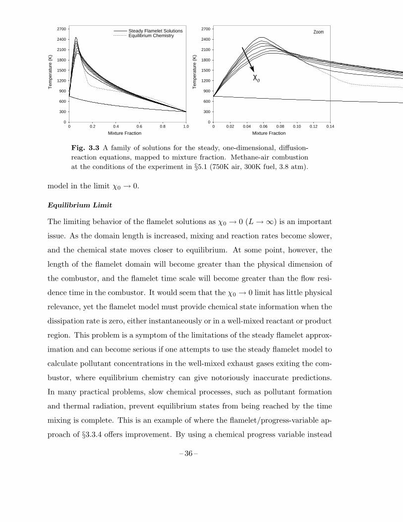
By varying the domain length, L, a one-parameter family of steady flamelet

solutions is obtained. The entire family of solutions is compiled into a flamelet

library , to yield chemical state relationships of the form,

yi = yi(Z, χ0) , T = T (Z, χ0) , ρ = ρ(Z, χ0) , (3.37)

where the solution dependence on L has been remapped to the dissipation rate

parameter, χ0, which varies monotonically with L. An example of a flamelet library

is depicted in Fig. 3.3, where T (Z, χ0) is plotted for several values of χ0. Also shown

is the equilibrium temperature curve from Fig. 3.1. It is apparent from the figure

that equilibrium chemistry can be obtained as a special case of the steady flamelet

– 35 –

Mixture Fraction

Tem

pera

ture

(K

)

0 0.2 0.4 0.6 0.8 1.00

300

600

900

1200

1500

1800

2100

2400

2700 Steady Flamelet SolutionsEquilibrium Chemistry

Mixture Fraction

Tem

pera

ture

(K

)

0 0.02 0.04 0.06 0.08 0.10 0.12 0.140

300

600

900

1200

1500

1800

2100

2400

2700Zoom

χ0

Fig. 3.3 A family of solutions for the steady, one-dimensional, diffusion-

reaction equations, mapped to mixture fraction. Methane-air combustion

at the conditions of the experiment in §5.1 (750K air, 300K fuel, 3.8 atm).

model in the limit χ0 → 0.

Equilibrium Limit

The limiting behavior of the flamelet solutions as χ0 → 0 (L→∞) is an important

issue. As the domain length is increased, mixing and reaction rates become slower,

and the chemical state moves closer to equilibrium. At some point, however, the

length of the flamelet domain will become greater than the physical dimension of

the combustor, and the flamelet time scale will become greater than the flow resi-

dence time in the combustor. It would seem that the χ0 → 0 limit has little physical

relevance, yet the flamelet model must provide chemical state information when the

dissipation rate is zero, either instantaneously or in a well-mixed reactant or product

region. This problem is a symptom of the limitations of the steady flamelet approx-

imation and can become serious if one attempts to use the steady flamelet model to

calculate pollutant concentrations in the well-mixed exhaust gases exiting the com-

bustor, where equilibrium chemistry can give notoriously inaccurate predictions.

In many practical problems, slow chemical processes, such as pollutant formation

and thermal radiation, prevent equilibrium states from being reached by the time

mixing is complete. This is an example of where the flamelet/progress-variable ap-

proach of §3.3.4 offers improvement. By using a chemical progress variable instead

– 36 –

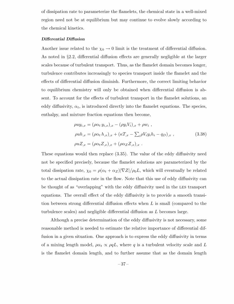
of dissipation rate to parameterize the flamelets, the chemical state in a well-mixed

region need not be at equilibrium but may continue to evolve slowly according to

the chemical kinetics.

Differential Diffusion

Another issue related to the χ0 → 0 limit is the treatment of differential diffusion.

As noted in §2.2, differential diffusion effects are generally negligible at the larger

scales because of turbulent transport. Thus, as the flamelet domain becomes longer,

turbulence contributes increasingly to species transport inside the flamelet and the

effects of differential diffusion diminish. Furthermore, the correct limiting behavior

to equilibrium chemistry will only be obtained when differential diffusion is ab-

sent. To account for the effects of turbulent transport in the flamelet solutions, an

eddy diffusivity, αt, is introduced directly into the flamelet equations. The species,

enthalpy, and mixture fraction equations then become,

ρuyi,x = (ραt yi,x),x − (ρyiVi),x + ρwi ,

ρuh,x = (ραt h,x),x + (κT,x −∑

iρViyihi − qD),x ,

ρuZ,x = (ραtZ,x),x + (ραZZ,x),x .

(3.38)

These equations would then replace (3.35). The value of the eddy diffusivity need

not be specified precisely, because the flamelet solutions are parameterized by the

total dissipation rate, χ0 = ρ(αt + αZ)|∇Z|/ρ0L, which will eventually be related

to the actual dissipation rate in the flow. Note that this use of eddy diffusivity can

be thought of as “overlapping” with the eddy diffusivity used in the les transport

equations. The overall effect of the eddy diffusivity is to provide a smooth transi-

tion between strong differential diffusion effects when L is small (compared to the

turbulence scales) and negligible differential diffusion as L becomes large.

Although a precise determination of the eddy diffusivity is not necessary, some

reasonable method is needed to estimate the relative importance of differential dif-

fusion in a given situation. One approach is to express the eddy diffusivity in terms

of a mixing length model, ραt ∝ ρqL, where q is a turbulent velocity scale and L

is the flamelet domain length, and to further assume that as the domain length

– 37 –

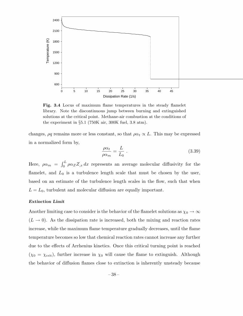
Dissipation Rate (1/s)

Tem

pera

ture

(K

)

0 5 10 15 20 25 30 35 40 45

600

900

1200

1500

1800

2100

2400

Fig. 3.4 Locus of maximum flame temperatures in the steady flamelet

library. Note the discontinuous jump between burning and extinguished

solutions at the critical point. Methane-air combustion at the conditions of

the experiment in §5.1 (750K air, 300K fuel, 3.8 atm).

changes, ρq remains more or less constant, so that ραt ∝ L. This may be expressed

in a normalized form by,ραtραm

=L

L0. (3.39)

Here, ραm =∫ L0ραZZ,x dx represents an average molecular diffusivity for the

flamelet, and L0 is a turbulence length scale that must be chosen by the user,

based on an estimate of the turbulence length scales in the flow, such that when

L = L0, turbulent and molecular diffusion are equally important.

Extinction Limit

Another limiting case to consider is the behavior of the flamelet solutions as χ0 →∞(L → 0). As the dissipation rate is increased, both the mixing and reaction rates

increase, while the maximum flame temperature gradually decreases, until the flame

temperature becomes so low that chemical reaction rates cannot increase any further

due to the effects of Arrhenius kinetics. Once this critical turning point is reached

(χ0 = χcrit), further increase in χ0 will cause the flame to extinguish. Although

the behavior of diffusion flames close to extinction is inherently unsteady because

– 38 –

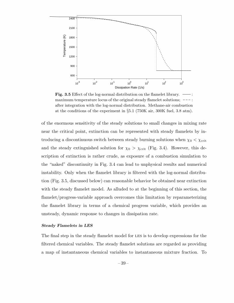
Dissipation Rate (1/s)

Tem

pera

ture

(K

)

10-3

10-2

10-1

100

101

102

103

600

900

1200

1500

1800

2100

2400

Fig. 3.5 Effect of the log-normal distribution on the flamelet library. :

maximum temperature locus of the original steady flamelet solutions; :

after integration with the log-normal distribution. Methane-air combustion

at the conditions of the experiment in §5.1 (750K air, 300K fuel, 3.8 atm).

of the enormous sensitivity of the steady solutions to small changes in mixing rate

near the critical point, extinction can be represented with steady flamelets by in-

troducing a discontinuous switch between steady burning solutions when χ0 < χcrit

and the steady extinguished solution for χ0 > χcrit (Fig. 3.4). However, this de-

scription of extinction is rather crude, as exposure of a combustion simulation to

the “naked” discontinuity in Fig. 3.4 can lead to unphysical results and numerical

instability. Only when the flamelet library is filtered with the log-normal distribu-

tion (Fig. 3.5, discussed below) can reasonable behavior be obtained near extinction

with the steady flamelet model. As alluded to at the beginning of this section, the

flamelet/progress-variable approach overcomes this limitation by reparameterizing

the flamelet library in terms of a chemical progress variable, which provides an

unsteady, dynamic response to changes in dissipation rate.

Steady Flamelets in LES

The final step in the steady flamelet model for les is to develop expressions for the

filtered chemical variables. The steady flamelet solutions are regarded as providing

a map of instantaneous chemical variables to instantaneous mixture fraction. To

– 39 –

account for subgrid fluctuations in mixture fraction and dissipation rate, filtered

combustion variables are obtained by integrating (3.37) over the joint pdf of subgrid

Z and χ0 fluctuations. For example,

yi =

∫yi(Z, χ0)P (Z, χ0) dZ dχ0 . (3.40)

The joint pdf is modeled by first assuming that Z and χ0 are independent,

P (Z, χ0) = P (Z)P (χ0) . (3.41)

Then, P (Z) is modeled using the assumed beta pdf of §3.2.4, while P (χ0) is modeled

by another type of assumed pdf, the one-parameter log-normal distribution,

P (χ0) = LogNormal(χ0; χ, 1) , (3.42)

where,

LogNormal(x; µ, σ) =1

xσ√2π

exp−[ln(x)− µ]2

2σ2. (3.43)

The distribution mean and variance are related to the parameters µ and σ by,

x = eµ+1

2σ2

, x′2 = x2(eσ2 − 1) .

The log-normal distribution has been found in numerical experiments to provide

an accurate description of gradient magnitude and dissipation rate fluctuations of

conserved scalars in fully developed turbulence (Jimenez et al. 1997), although the

most appropriate value for σ is still an open question. For the present study a

value of σ = 1 was chosen. Figure 3.5 shows the filtering effect of the log-normal

distribution on the flamelet library.

Once the flamelet library is computed and assumed pdf integrals are evaluated,

lookup tables can be generated to provide the filtered chemical variables as functions

of the quantities readily available from les (namely, Z, Z ′′2, and χ):

yi = yi(Z, Z ′′2, χ) , T = T (Z, Z ′′2, χ) , ρ = ρ(Z, Z ′′2, χ) , etc. (3.44)

Note that (3.44) includes similar expressions for filtered transport properties such as

µ and αZ , which are used in solving the large-scale momentum and scalar transport

equations. The computational cost of the steady flamelet model is very modest,

because the functions in (3.44) can be precomputed and tabulated prior to running

a simulation.

– 40 –

3.3.4 The Flamelet/Progress-Variable Approach

The philosophy underlying the chemical models developed in this work is that the

most effective description of turbulent combustion will map the details of the multi-

component diffusion-reaction processes to a minimum set of transported “tracking”

scalars. Extensive discussion of the mixture fraction’s role as a tracking scalar was

given in §3.3.1. There it was also pointed out that a model based on mixture frac-

tion alone is incomplete, because mixture fraction does not contain any intrinsic

information about chemical reactions and cannot account for chemical variations in

directions perpendicular to its gradient. At least one additional scalar is needed,

and since mixture fraction accounts for transport of conserved scalars, additional

tracking scalars must be nonconserved in order to be independent from mixture frac-

tion. A nonconserved tracking scalar is best characterized as a reaction progress

variable.

Model Derivation

In the present work, addition of a single progress variable, generically denoted by

C, is considered. The set of scalar transport equations carried in a simulation is

then given by,

∂ρZ

∂t+∇ · (ρuZ) = ∇ · (ραZ∇Z) ,

∂ρC

∂t+∇ · (ρuC) = ∇ · (ραC∇C) + ρwC .

(3.45)

Complete chemical state information is to be derived from Z and C through chem-

ical state relationships of the form,

yi = yi(Z,C) , T = T (Z,C) , ρ = ρ(Z,C) . (3.46)

In particular, the chemical source for the progress variable, which is a function of

the chemical state, will be given by wC = wC(Z,C). The remaining question is how

to determine the best chemical state relationships for a given case. A very simple

approach, developed for the present study and discussed below, is to use the steady

flamelet state relationships (3.37) of §3.3.3.

– 41 –

Consider a computational experiment, in which a reacting flow is simulated

using the steady flamelet model of §3.3.3. However, suppose that in addition to

mixture fraction, a transport equation is solved for one of the chemical species,

with the reaction source term for the species calculated from the chemical states

predicted by the steady flamelet model. This situation leads naturally to the follow-

ing questions: Would the species concentrations obtained by solving the additional

transport equation be any different from those predicted by the steady flamelet

model alone? And if the transport equation solution were more accurate than the

steady flamelet prediction, could it not be used to constrain or parameterize the

steady flamelet model? To be more specific, suppose that the transported species

in question is actually the previously introduced progress variable. Then, the set of

transport equations being solved is given in (3.45), while the steady flamelet model

(3.37) predicts,

C = C(Z, χ0) , (3.47)

giving us two independent equations for the progress variable. If (3.47) is to be

consistent with (3.45), χ0 can no longer be coupled directly to the local dissipation

rate in the flow, but instead must be constrained by (3.47). Provided that the

progress variable varies monotonically with χ0, (3.47) can be inverted to obtain,

χ0 = χ0(Z,C) . (3.48)

Substituting this into (3.37) yields (3.46).

Unsteady Flamelet Interpretation

The flamelet/progress-variable approach can alternatively be derived by interpreting

it as a type of unsteady flamelet model. Since the dissipation rate parameter, χ0,

is determined in (3.48) by the value of the progress variable and does not have

any direct relationship to the actual dissipation rate in the flow, it should not be

regarded as representing a real dissipation rate but rather a ficticious one, which we

denote by χ′. Thus, the flamelet equations used in the flamelet/progress-variable

approach are given by

ρχ′d2yidZ2

= −ρwi , (3.49)

– 42 –

where χ′ = χ′(Z,C) and in general, χ′ 6= χ. If we now add and subtract the term

χ(d2yi/dZ2) in (3.49), it can be written in the form,

ρ(χ− χ′)d2yidZ2

= ρχd2yidZ2

+ ρwi . (3.50)

Meanwhile, the unsteady flamelet equations (Peters 1984) are given by:

ρ∂yi∂t

= ρχ∂2yi∂Z2

+ ρwi . (3.51)

Comparing (3.50) with (3.51), it is apparent that the left-hand side of (3.50) can

be interpreted as a type of unsteady term in the flamelet equations:

ρ∂yi∂t

≈ ρ(χ− χ′)d2yidZ2

, (3.52)

where the difference between the actual and ficticious dissipation rates indicates the

degree of unsteadiness. This form for the unsteady term appears as a relaxation

mechanism, evolving the flamelet solution ever closer to the steady flamelet solution

for the given dissipation rate, χ. In this sense, χ′ can be thought of as a lagging

dissipation rate containing the memory of the flame structure from an earlier time

when χ and χ′ were equal. This concept, of a ficticious dissipation rate that rep-

resents the history of the evolution of the flamelet, is similar to the “equivalent”

strain rate of Cuenot et al. (2000). It should be noted that the unsteady evolution

suggested by (3.52) is actually embedded in the progress-variable transport equa-

tion, where the reaction and dissipation rates directly affect the evolution of the

progress variable in a manner similar to (3.51).

Application to LES

So far, the derivation of the flamelet/progress-variable approach has been in terms of

fully resolved, instantaneous quantities without consideration of subgrid turbulence

modeling. This is to separate the assumptions involved in the chemistry model

from those used in the turbulence model. When written in terms of filtered les

quantities, (3.45) becomes,

∂ρZ

∂t+∇ · (ρuZ) = ∇ · [ρ(αZ + αt)∇Z] ,

∂ρC

∂t+∇ · (ρuC) = ∇ · [ρ(αC + αt)∇C] + ρwC ,

(3.53)

– 43 –

where αt is the turbulent diffusivity of §3.2.2. To account for subgrid fluctuations

in the mixture fraction and progress variable, filtered combustion variables are ob-

tained by integrating (3.46) over the joint pdf of Z and C. For example,

yi =

∫yi(Z,C)P (Z,C) dZ dC , (3.54)

and,

wC =

∫wC(Z,C)P (Z,C) dZ dC . (3.55)

The joint pdf is modeled by first writing,

P (Z,C) = P (C|Z)P (Z) , (3.56)

where P (Z) is given by the assumed beta pdf of §3.2.4. The conditional pdf,

P (C|Z), is modeled by assuming that each subgrid chemical state is represented by

a single flamelet solution. Mathematically this is described by a delta function,

P (C|Z) = δ(C − C|Z) , (3.57)

where the conditional mean, C|Z, is given by one of the steady flamelet solutions

in (3.37),

C|Z = C(Z, χ0) , (3.58)

and χ0 is chosen such that the constraint,

C =

∫C(Z, χ0)P (Z) dZ , (3.59)

analogous to (3.47), is satisfied. The flamelet/progress-variable approach could

benefit from a more sophisticated model for P (C|Z), but as noted in §3.2.4, assumed

pdf modeling of reacting scalars needs to be further researched.

The implementation of the flamelet/progress-variable approach is similar to the

steady flamelet model in that it employs chemical state relationships determined by

a flamelet library and uses assumed pdf’s to represent subgrid fluctuations. The

major difference, of course, is the parameterization by a progress variable instead

– 44 –

of dissipation rate. Once the flamelet library is computed and assumed pdf inte-

grals are evaluated, lookup tables can be generated to provide the filtered chemical

variables as functions of the quantities readily available from les (namely, Z, Z ′′2,

and C):

yi = yi(Z, Z ′′2, C) , T = T (Z, Z ′′2, C) , ρ = ρ(Z, Z ′′2, C) , etc. (3.60)

Note that (3.60) includes similar expressions for µ, αZ , αC , and wC , which are

used in solving the large-scale momentum and scalar transport equations. The

computational cost of the flamelet/progress-variable approach is only marginally

greater than the steady flamelet model, because the functions in (3.60) can be

precomputed and tabulated prior to running a simulation. The major additional

cost comes from solving the transport equation for the progress variable.

Further Discussion

One of the more conspicuous limitations of the steady flamelet model (§3.3.3) is itsinability to properly account for ignition and extinction phenomena. This is ex-

emplified most clearly by the discontinuous jump in flame states in Fig. 3.4, which

indicates that the steady flamelet library is somehow incomplete because it can-

not represent any of the “partially extinguished” intermediate states that should

fill the gap between the critical point and complete extinction. In fact, the steady

flamelet equations do provide a complete and continuous set of solutions rang-

ing from chemical equilibrium to complete extinction, but they are not in general

uniquely parameterized by the dissipation rate.

The complete locus of solutions to the steady flamelet equations is shown in

Fig. 3.6. The shape of this curve, sometimes called the “S-shaped curve” in diffu-

sion flame theory, is determined primarily by the chemical kinetics. With Arrhenius

kinetics, there are typically three solution branches: (1) the steady burning branch,

(2) the unstable branch of partially extinguished states, and (3) the complete ex-

tinction line. On the stable burning branch, maximum flame temperature decreases

with increasing dissipation rate as more rapid mixing increases reactant concen-

trations while diluting product concentrations. When the critical point is reached,

– 45 –

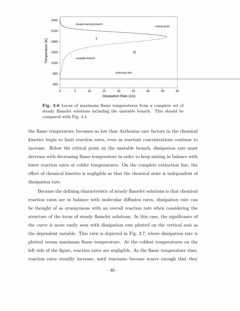
Dissipation Rate (1/s)

Tem

pera

ture

(K

)

0 5 10 15 20 25 30 35 40

600

900

1200

1500

1800

2100

2400

I

II

steady burning branch

unstable branch

extinction line

critical point

Fig. 3.6 Locus of maximum flame temperatures from a complete set of

steady flamelet solutions including the unstable branch. This should be

compared with Fig. 3.4.

the flame temperature becomes so low that Arrhenius rate factors in the chemical

kinetics begin to limit reaction rates, even as reactant concentrations continue to

increase. Below the critical point on the unstable branch, dissipation rate must

decrease with decreasing flame temperature in order to keep mixing in balance with

lower reaction rates at colder temperatures. On the complete extinction line, the

effect of chemical kinetics is negligible so that the chemical state is independent of

dissipation rate.

Because the defining characteristic of steady flamelet solutions is that chemical

reaction rates are in balance with molecular diffusion rates, dissipation rate can

be thought of as synonymous with an overall reaction rate when considering the

structure of the locus of steady flamelet solutions. In this case, the significance of

the curve is more easily seen with dissipation rate plotted on the vertical axis as

the dependent variable. This view is depicted in Fig. 3.7, where dissipation rate is

plotted versus maximum flame temperature. At the coldest temperatures on the

left side of the figure, reaction rates are negligible. As the flame temperature rises,

reaction rates steadily increase, until reactants become scarce enough that they

– 46 –

Temperature (K)

Dis

sipa

tion

Rat

e (1

/s)

600 900 1200 1500 1800 2100 24000

10

20

30

40

Fig. 3.7 Locus of maximum flame temperatures viewed as reaction rate

versus temperature.

begin to limit reaction rates. Beyond this point, reaction rates steadily decrease as

the chemical state approaches equilibrium on the right side of the figure.

The use of the unstable branch of steady flamelet solutions in the progress

variable approach has been criticized as unphysical, but as we now demonstrate,

the behavior of the model in this region is very similar to that of an unsteady

flamelet solution. For a given maximum flame temperature on the vertical axis of

Fig. 3.6, the ficticious dissipation rate, χ′, corresponds to a point on the curve,

while the actual dissipation rate, χ, will correspond to a location either in region

I or in region II, depending on whether χ < χ′ or χ > χ′, respectively. Referring

to (3.52) and noting that d2T/dZ2 is negative in the region where temperature is

maximum, we see that in region I, the unsteady term is positive,

∂T

∂t≈ (χ− χ′)d

2T

dZ2> 0 in region I ,

so that the flame state moves up to the steady burning solution branch, while in

region II, the unsteady term is negative,

∂T

∂t≈ (χ− χ′)d

2T

dZ2< 0 in region II ,

so that the flame state moves down to the steady extinguished solution branch (or

down to the steady burning branch if it is initially above it). Thus, the unstable

– 47 –

solution branch is important both physically and in the progress-variable approach

because it delineates the border between regions I and II, between ignition and

extinction of the flame.

The last issue we consider is the definition of the progress variable. For a

one-step chemical mechanism, there is only a single degree of freedom remaining

after mixture fraction is known, so that any species, be it fuel, oxidizer, or product,

uniquely determines the others and can be chosen to serve as the progress variable.

In fact, the progress-variable approach provides an exact description of one-step

chemical systems. But for a large, multistep chemical system, the selection of the

progress variable should be guided by the two following criteria: (1) the progress

variable should be an important, controlling quantity that contains the essential

features of the process it is supposed to represent, and (2) it should provide a unique

mapping of all of the chemical states in the flamelet library. The dissipation rate is

an example of a quantity that clearly does not uniquely determine chemical states

(Fig. 3.6). Similarly, intermediate species that are produced and later consumed are

not expected to be useful indicators of reaction progress. Since the final result of

chemical reactions is to transform reactants into products, a good measure of how

far the transformation has progressed is the product mass fraction. In the present

study, the progress variable defined by C = yP = yCO2+ yH2O is used for the case

of methane-air combustion. However, product mass fraction does not necessarily

satisfy the second criterion of providing a unique mapping of all the states. For

methane-air combustion, there is a significant region of nonuniqueness in fuel-rich

mixtures close to equilibrium, similar to what is seen in the temperature in Fig. 3.3.

In practice, the solution to this problem is to use a “truncated” flamelet library,

in which the nonunique, near-equilibrium states are removed. Unfortunately, this

approximation may break down in regions where hot products mix with unburned

fuel and may explain the discrepancy in the carbon monoxide prediction in Fig. 5.9.

In general, the only chemical property that is guaranteed to vary monotonically

during chemical reactions is the entropy, and so this would be a logical choice

for the progress variable. However, entropy is governed by a significantly more

– 48 –

complicated equation than (3.45) and includes source terms for both mixing and

chemical reaction. Nevertheless, future studies using a progress-variable approach

should consider using entropy as the progress variable.

– 49 –

– 50 –

Chapter 4

NUMERICAL METHODS

One of the main objectives of this work was the development of special numerics for large

eddy simulation of variable-density flows with heat release. Typical numerical methods

used in computational fluid dynamics are usually not suitable for les because they do

not consider the important issue of nonlinear stability. This chapter discusses a staggered

space-time, conservative discretization for the variable-density transport equations, as well

as an efficient, semi-implicit iterative technique for integrating those equations. Details of

the implementation in cylindrical coordinates and the specification of boundary conditions

are also considered.

4.1 Conservative Space-Time Discretization

Large eddy simulations are more vulnerable to numerical errors than most other

types of numerical computation (such as direct numerical simulations) because prac-

tical calculations are always under-resolved. While subgrid-scale models may ac-

count for the effects of unresolved physical scales, they should not be expected to

compensate for numerical errors. Consequently, practical large eddy simulations

can “blow up” when aliasing or other errors contaminate the solution. The typical

remedy is to incorporate some form of artificial dissipation (such as upwind biased

schemes or explicit filtering techniques) to damp instabilities and other numerical

errors. Unfortunately, this approach usually leads to the unwanted damping of

physical processes as well as numerical errors, especially when a broadband range

of nonlinearly interacting scales is simulated. Even if artificial dissipation is care-

fully confined to the smallest scales, larger scales will still be indirectly affected

through nonlinear interactions. Fortunately, stability can be achieved without ar-

tificial damping by designing numerical schemes to satisfy certain conservation re-

quirements.

– 51 –

4.1.1 The Role of Conservation

Consider the Eulerian transport equation for a conserved quantity η,

∂ρη

∂t+∇ · (ρuη) = 0 , (4.1)

and the continutity equation (obtained with η = 1),

∂ρ

∂t+∇ · (ρu) = 0 . (4.2)

These equations directly express the (primary) conservation of η and of mass, but

together, they also imply conservation of any function, f(η):

∂ρf(η)

∂t+∇ · [ρuf(η)] = 0 . (4.3)

In particular, the function f(η) = 12η2 or “η-energy” is also conserved. This is

refered to as secondary conservation. From the point of view of numerical methods,

secondary conservation is what guarantees nonlinear stability.

Because the continuity equation for variable-density flows contains a time

derivative term, one needs to consider both temporal and spatial discretizations

when developing conservative schemes. That is, the temporal and spatial deriva-

tives in the material convection terms must be discretized in a specific relation to

each other and to the time-dependent continuity equation. This is clear from the

steps required to derive (4.3) from (4.1) and (4.2). In the following sections, discrete

analogs of the product rule of differentiation in calculus will be used to show how

both primary and secondary conservation can be achieved in the discrete equations.

4.1.2 Index-Free Notation

Before presenting the discrete equations, we introduce a compact and convenient

notation for writing discretized equations in a form similar to the original partial

differential equations (Piacsek and Williams 1970; Morinishi et al. 1998). This

notation is also very useful for performing algebraic manipulations on the equations.

– 52 –

Second-order discretizations usually involve the primitive operations of inter-

polation and differencing in a particular coordinate direction. For any pair of coor-

dinate directions x and y having uniform grids with respective spacings ∆x and ∆y

and respective grid indices i and j, we define the interpolation operators,

ux∣∣∣i,j

=ui+1/2,j + ui−1/2,j

2, uy

∣∣∣i,j

=ui,j+1/2 + ui,j−1/2

2, (4.4)

and the differencing operators,

δx(u)∣∣∣i,j

=ui+1/2,j − ui−1/2,j

∆x, δy(u)

∣∣∣i,j

=ui,j+1/2 − ui,j−1/2

∆y. (4.5)

Note that each of the operators in (4.4) and (4.5) produces a result that is staggered

with respect to the operand in the coordinate direction indicated. For example, ux

is shifted 12∆x with respect to u in the x direction. We also define the following

nonlinear interpolation operator:

uvx= 2uxvx − uvx , (4.6)

which will be used in the expressions of secondary conservation.

There are a number of discrete identities, easily proved by substitution of the

above definitions, which will be useful later:

δx(abx) = aδx(b)

x+ b δx(a) , (4.7)

δx(ab) = axδx(b) + bxδx(a) , (4.8)

δx(ay) = δx(a)

y, (4.9)

axy= ay

x. (4.10)

Here, a and b are any two compatible quantities and x and y are any two coordinate

directions. Two quantities are compatible if the locations at which they are defined

have the proper relationship for the expression to make sense. All terms that

multiply or add in a given expression must be defined on the same set of grid

points (not staggered with respect to one another). For example, the product

– 53 –

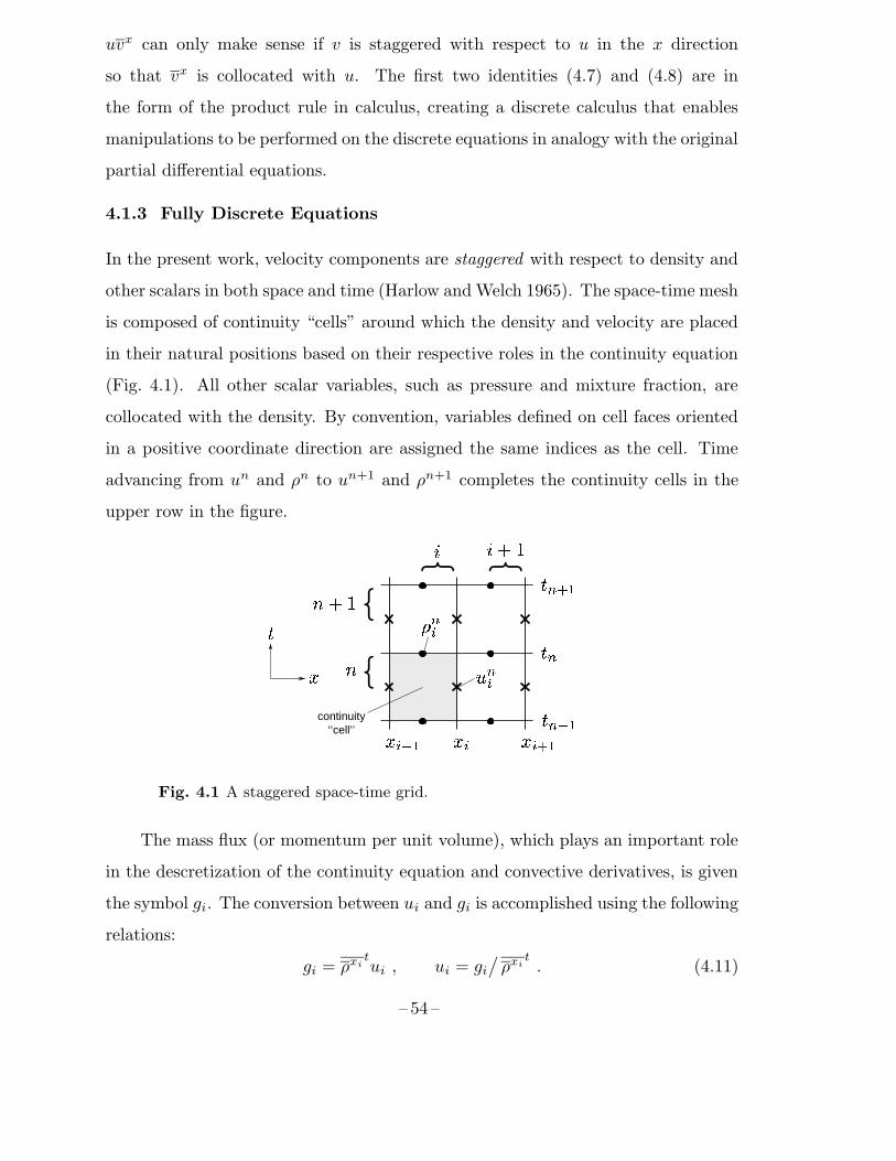
uvx can only make sense if v is staggered with respect to u in the x direction

so that vx is collocated with u. The first two identities (4.7) and (4.8) are in

the form of the product rule in calculus, creating a discrete calculus that enables

manipulations to be performed on the discrete equations in analogy with the original

partial differential equations.

4.1.3 Fully Discrete Equations

In the present work, velocity components are staggered with respect to density and

other scalars in both space and time (Harlow andWelch 1965). The space-time mesh

is composed of continuity “cells” around which the density and velocity are placed

in their natural positions based on their respective roles in the continuity equation

(Fig. 4.1). All other scalar variables, such as pressure and mixture fraction, are

collocated with the density. By convention, variables defined on cell faces oriented

in a positive coordinate direction are assigned the same indices as the cell. Time

advancing from un and ρn to un+1 and ρn+1 completes the continuity cells in the

upper row in the figure.

���

�������

���� ��� ��������������

�

�

continuity‘‘cell’’

{�! #"

$ {

%'&#({){

*,+-

.0/1

Fig. 4.1 A staggered space-time grid.

The mass flux (or momentum per unit volume), which plays an important role

in the descretization of the continuity equation and convective derivatives, is given

the symbol gi. The conversion between ui and gi is accomplished using the following

relations:

gi = ρxitui , ui = gi

/ρxi

t. (4.11)

– 54 –

In direct analogy with (2.20–2.22), we now present the fully discrete equations.

Note that interpolation operators (overbars with superscripts) do not follow the

summation convention.

Continuity:

δt(ρ) + δxj(gj) = 0 (4.12)

Momentum:

δt(gi) + δxj(gj

xituixjt) = −δxi

(p) + δxj(τij) (4.13)

τij =

{µxi

xj[δxj

(uit) + δxi

(ujt)]

i 6= j2µ[δxj

(uit)− 1

3δxk

(ukt)δij ] i = j

Scalar Transport:

δt(ρφ) + δxj(gjφ

xjt

) = δxj

[ραxj

tδxj

(φt)]+ ρtw(φ

t) . (4.14)

For clarity we have dropped the scalar index k from the scalar transport equation.

The above compact notation can be expanded into more conventional form. For

example, the continuity equation in two dimensions for the cell above the shaded

one in Fig. 4.1 would be expanded as,

ρn+1i,j − ρni,j∆t

+1

4∆x

[(ρn+1i+1,j + ρn+1i,j + ρni+1,j + ρni,j)u

n+1i,j

− (ρn+1i,j + ρn+1i−1,j + ρni,j + ρni−1,j)un+1i−1,j

]

+1

4∆y

[(ρn+1i,j+1 + ρn+1i,j + ρni,j+1 + ρni,j)v

n+1i,j

− (ρn+1i,j + ρn+1i,j−1 + ρni,j + ρni,j−1)vn+1i,j−1

]= 0 .

When the above equations are generalized for nonuniform (stretched) grids,

the interpolation and differencing operators are defined as,

ux∣∣∣i+1/2

= ciui+1 + (1− ci)ui , δx(u)∣∣∣i+1/2

=ui+1 − uixi+1 − xi

, (4.15)

where ci are linear interpolation weights. These definitions maintain formal second-

order accuracy of the interpolation operator, but they do not satisfy the discrete

product rules exactly so that secondary conservation is only approximately satisfied.

In practice, the simulations are found to be stable on sufficiently smooth grids. A

more robust, but possibly less accurate, approach would be to continue using equal

weighted interpolations.

– 55 –

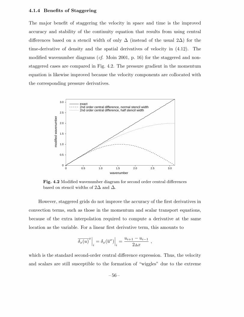
4.1.4 Benefits of Staggering

The major benefit of staggering the velocity in space and time is the improved

accuracy and stability of the continuity equation that results from using central

differences based on a stencil width of only ∆ (instead of the usual 2∆) for the

time-derivative of density and the spatial derivatives of velocity in (4.12). The

modified wavenumber diagrams (cf. Moin 2001, p. 16) for the staggered and non-

staggered cases are compared in Fig. 4.2. The pressure gradient in the momentum

equation is likewise improved because the velocity components are collocated with

the corresponding pressure derivatives.

wavenumber

mod

ified

wav

enum

ber

0 0.5 1.0 1.5 2.0 2.5 3.00

0.5

1.0

1.5

2.0

2.5

3.0exact2nd order central difference, normal stencil width2nd order central difference, half stencil width

Fig. 4.2 Modified wavenumber diagram for second order central differences

based on stencil widths of 2∆ and ∆.

However, staggered grids do not improve the accuracy of the first derivatives in

convection terms, such as those in the momentum and scalar transport equations,

because of the extra interpolation required to compute a derivative at the same

location as the variable. For a linear first derivative term, this amounts to

δx(u)x∣∣∣i= δx(u

x)∣∣∣i=ui+1 − ui−1

2∆x,

which is the standard second-order central difference expression. Thus, the velocity

and scalars are still susceptible to the formation of “wiggles” due to the extreme

– 56 –

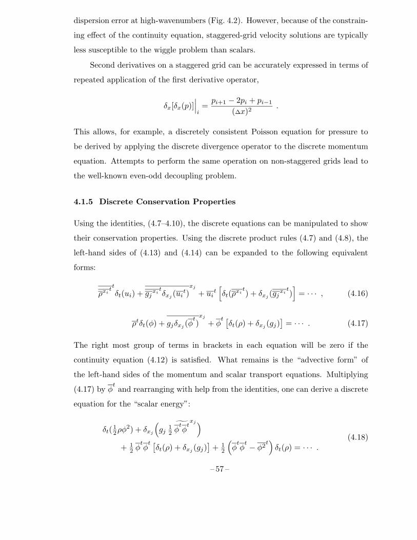
dispersion error at high-wavenumbers (Fig. 4.2). However, because of the constrain-

ing effect of the continuity equation, staggered-grid velocity solutions are typically

less susceptible to the wiggle problem than scalars.

Second derivatives on a staggered grid can be accurately expressed in terms of

repeated application of the first derivative operator,

δx[δx(p)]∣∣∣i=pi+1 − 2pi + pi−1

(∆x)2.

This allows, for example, a discretely consistent Poisson equation for pressure to

be derived by applying the discrete divergence operator to the discrete momentum

equation. Attempts to perform the same operation on non-staggered grids lead to

the well-known even-odd decoupling problem.

4.1.5 Discrete Conservation Properties

Using the identities, (4.7–4.10), the discrete equations can be manipulated to show

their conservation properties. Using the discrete product rules (4.7) and (4.8), the

left-hand sides of (4.13) and (4.14) can be expanded to the following equivalent

forms:

ρxitt

δt(ui) + gjxitδxj

(uit)xj

+ uit[δt(ρ

xit) + δxj

(gjxit)]= · · · , (4.16)

ρtδt(φ) + gjδxj(φ

t)xj

+ φt [δt(ρ) + δxj

(gj)]= · · · . (4.17)

The right most group of terms in brackets in each equation will be zero if the

continuity equation (4.12) is satisfied. What remains is the “advective form” of

the left-hand sides of the momentum and scalar transport equations. Multiplying

(4.17) by φtand rearranging with help from the identities, one can derive a discrete

equation for the “scalar energy”:

δt(12ρφ2) + δxj

(gj12φtφtxj)

+ 12φtφt [δt(ρ) + δxj

(gj)]+ 12

(φtφt − φ2t

)δt(ρ) = · · · .

(4.18)

– 57 –

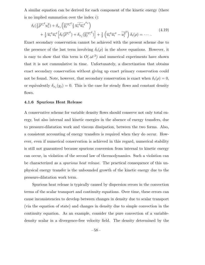
A similar equation can be derived for each component of the kinetic energy (there

is no implied summation over the index i):

δt(12ρxi

tu2i ) + δxj

(gjxit 12˜uituit

xj)

+ 12uitui

t[δt(ρ

xit) + δxj

(gjxit)]+ 12

(uitui

t − u2it)δt(ρ) = · · · .

(4.19)

Exact secondary conservation cannot be achieved with the present scheme due to

the presence of the last term involving δt(ρ) in the above equations. However, it

is easy to show that this term is O(∆t 2) and numerical experiments have shown

that it is not cummulative in time. Unfortunately, a discretization that obtains

exact secondary conservation without giving up exact primary conservation could

not be found. Note, however, that secondary conservation is exact when δt(ρ) = 0,

or equivalently δxj(gj) = 0. This is the case for steady flows and constant density

flows.

4.1.6 Spurious Heat Release

A conservative scheme for variable density flows should conserve not only total en-

ergy, but also internal and kinetic energies in the absence of energy transfers, due

to pressure-dilatation work and viscous dissipation, between the two forms. Also,

a consistent accounting of energy transfers is required when they do occur. How-

ever, even if numerical conservation is achieved in this regard, numerical stability

is still not guaranteed because spurious conversion from internal to kinetic energy

can occur, in violation of the second law of thermodynamics. Such a violation can

be characterized as a spurious heat release. The practical consequence of this un-

physical energy transfer is the unbounded growth of the kinetic energy due to the

pressure-dilatation work term.

Spurious heat release is typically caused by dispersion errors in the convection

terms of the scalar transport and continuity equations. Over time, these errors can

cause inconsistencies to develop between changes in density due to scalar transport

(via the equation of state) and changes in density due to simple convection in the

continuity equation. As an example, consider the pure convection of a variable-

density scalar in a divergence-free velocity field. The density determined by the

– 58 –

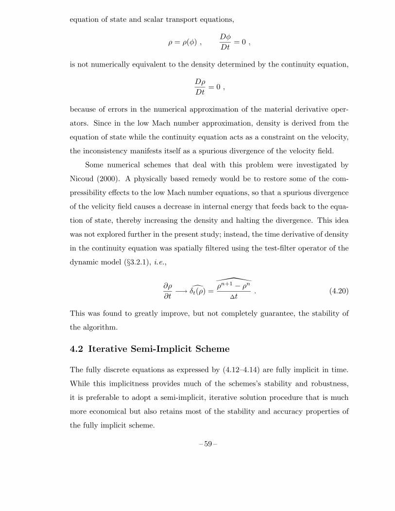
equation of state and scalar transport equations,

ρ = ρ(φ) ,Dφ

Dt= 0 ,

is not numerically equivalent to the density determined by the continuity equation,

Dρ

Dt= 0 ,

because of errors in the numerical approximation of the material derivative oper-

ators. Since in the low Mach number approximation, density is derived from the

equation of state while the continuity equation acts as a constraint on the velocity,

the inconsistency manifests itself as a spurious divergence of the velocity field.

Some numerical schemes that deal with this problem were investigated by

Nicoud (2000). A physically based remedy would be to restore some of the com-

pressibility effects to the low Mach number equations, so that a spurious divergence

of the velicity field causes a decrease in internal energy that feeds back to the equa-

tion of state, thereby increasing the density and halting the divergence. This idea

was not explored further in the present study; instead, the time derivative of density

in the continuity equation was spatially filtered using the test-filter operator of the

dynamic model (§3.2.1), i.e.,

∂ρ

∂t−→ δt(ρ) =

ρn+1 − ρn∆t

. (4.20)

This was found to greatly improve, but not completely guarantee, the stability of

the algorithm.

4.2 Iterative Semi-Implicit Scheme

The fully discrete equations as expressed by (4.12–4.14) are fully implicit in time.

While this implicitness provides much of the schemes’s stability and robustness,

it is preferable to adopt a semi-implicit, iterative solution procedure that is much

more economical but also retains most of the stability and accuracy properties of

the fully implicit scheme.

– 59 –

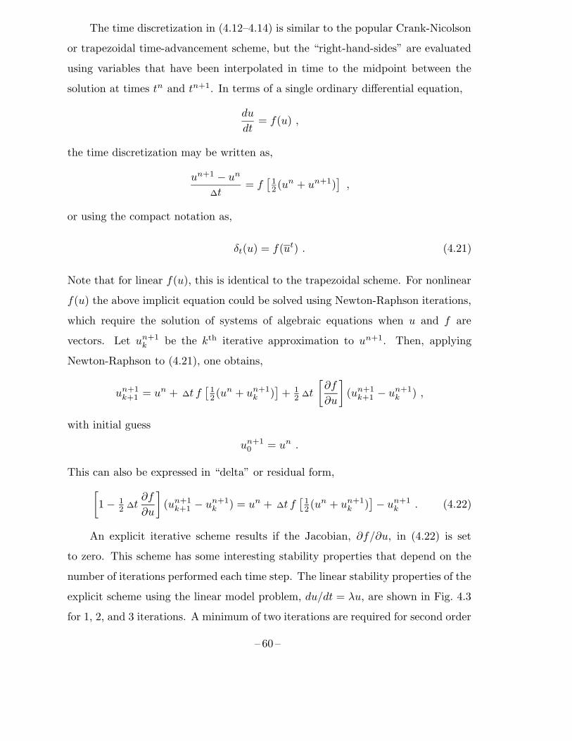
The time discretization in (4.12–4.14) is similar to the popular Crank-Nicolson

or trapezoidal time-advancement scheme, but the “right-hand-sides” are evaluated

using variables that have been interpolated in time to the midpoint between the

solution at times tn and tn+1. In terms of a single ordinary differential equation,

du

dt= f(u) ,

the time discretization may be written as,

un+1 − un∆t

= f[12(un + un+1)

],

or using the compact notation as,

δt(u) = f(ut) . (4.21)

Note that for linear f(u), this is identical to the trapezoidal scheme. For nonlinear

f(u) the above implicit equation could be solved using Newton-Raphson iterations,

which require the solution of systems of algebraic equations when u and f are

vectors. Let un+1k be the kth iterative approximation to un+1. Then, applying

Newton-Raphson to (4.21), one obtains,

un+1k+1 = un + ∆t f[12(un + un+1k )

]+ 12∆t

[∂f

∂u

](un+1k+1 − un+1k ) ,

with initial guess

un+10 = un .

This can also be expressed in “delta” or residual form,

[1− 1

2∆t

∂f

∂u

](un+1k+1 − un+1k ) = un + ∆t f

[12(un + un+1k )

]− un+1k . (4.22)

An explicit iterative scheme results if the Jacobian, ∂f/∂u, in (4.22) is set

to zero. This scheme has some interesting stability properties that depend on the

number of iterations performed each time step. The linear stability properties of the

explicit scheme using the linear model problem, du/dt = λu, are shown in Fig. 4.3

for 1, 2, and 3 iterations. A minimum of two iterations are required for second order

– 60 –

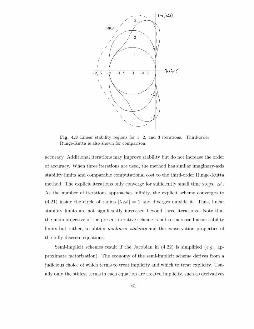
-2.5 -2 -1.5 -1 -0.5

-2

-1

1

2

-2.5 -2 -1.5 -1 -0.5

-2

-1

1

2

1

2

RK3

3

�����������

�����������

Fig. 4.3 Linear stability regions for 1, 2, and 3 iterations. Third-order

Runge-Kutta is also shown for comparison.

accuracy. Additional iterations may improve stability but do not increase the order

of accuracy. When three iterations are used, the method has similar imaginary-axis

stability limits and comparable computational cost to the third-order Runge-Kutta

method. The explicit iterations only converge for sufficiently small time steps, ∆t .

As the number of iterations approaches infinity, the explicit scheme converges to

(4.21) inside the circle of radius |λ∆t | = 2 and diverges outside it. Thus, linear

stability limits are not significantly increased beyond three iterations. Note that

the main objective of the present iterative scheme is not to increase linear stability

limits but rather, to obtain nonlinear stability and the conservation properties of

the fully discrete equations.

Semi-implicit schemes result if the Jacobian in (4.22) is simplified (e.g. ap-

proximate factorization). The economy of the semi-implicit scheme derives from a

judicious choice of which terms to treat implicity and which to treat explicity. Usu-

ally only the stiffest terms in each equation are treated implicity, such as derivatives

– 61 –

in a coordinate direction that has a much greater variation in grid spacing than the

other directions. For example, where grid refinement occurs near a wall, only deriva-

tives in the wall-normal direction would be treated implicitly. In the present study,

the following terms are treated implicitly: (1) advection and diffusion in the ra-

dial direction, (2) advection and diffusion in the azimuthal direction, and (3) the

pressure in all directions via a Poisson equation.

The iteration procedure employed in the present study is summarized below.

In the following, the superscript n refers to solution values that are known from

the previous time level, the superscript k refers to the iteration cycle between the

solutions at time step n and n + 1, the superscript 0 indicates the initial guess

for the first iteration when k = 0, and a hat placed above a symbol is used for a

provisional value of some quantity.

Step 1: Choose predictors (initial guesses) for the values of the variables at the

next time level. The simplest choice is to use the solution values at the current time

level:

u0i = uni , φ0 = φn , etc.

This choice corresponds to using explicit Euler (or first-order Runge-Kutta) for the

first iteration. Predictors are not essential to the present algorithm in that they do

not affect the final converged solution, but good predictors can speed convergence of

the iterations, and they can affect accuracy and stability when only a small number

of iterations are used. The density predictor is particularly important because it is

related to the conservation properties described in §4.1. Experience has shown that

it is best to ensure that the predictors for density and velocity satisfy the continuity

equation. That is, the predicted rate-of-change of density should correspond to the

predicted mass flux divergence. We therefore choose:

ρ0 = ρn − ∆t δxj(g0j ) .

With the predictor g0j = gnj , this is equivalent to linear extrapolation in time:

ρ0 = ρn + (ρn − ρn−1) = 2ρn − ρn−1 .

– 62 –

Step 2: We first advance the scalar equation(s) so that a better estimate for the

density can be obtained early in the iteration process. In the present work, each

scalar equation is updated separately, and semi-implicit penta-diagonal equations

(for the quick scheme discussed in §4.3) are solved for advection and diffusion in

the radial and azimuthal directions (using approximate factorization) so that grid

refinements in the radial direction near walls or in the azimuthal direction near

the centerline do not limit the time step. Any source terms are treated explicitly.

Time advancing (4.14) yields (ρφ)k+1, from which a provisonal estimate for φk+1 is

obtained using the current density predictor:

φ = (ρφ)k+1/ ρk .

Boundary conditions are enforced on φ.

Step 3: The density is updated from the equation of state, using the provisonal

scalar values:

ρk+1 = f(φ) .

Note that it may be possible in some cases to obtain ρk+1 directly as a function

of (ρφ)k+1. However, this was found to be less accurate because (ρφ)k+1 implicitly

contains ρk, which is based on information from the previous iteration.

Step 4: Re-update the scalar(s) based on the new density:

φk+1 = (ρφ)k+1/ ρk+1 .

This is required to preserve primary scalar conservation. Boundary conditions are

applied to φk+1.

Step 5: Time advance the momentum equations (4.13) to yield provisional es-

timates for the mass flux components, gi. In the present work, semi-implicit tri-

diagonal equations are solved separately for each velocity component for advection

and diffusion in the radial and azimuthal directions using approximate factoriza-

tion. The current best estimate for pressure is included on the right-hand-side.

– 63 –

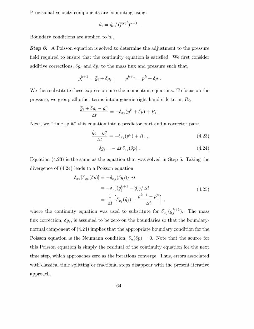
Provisional velocity components are computing using:

ui = gi / (ρxit)k+1 .

Boundary conditions are applied to ui.

Step 6: A Poisson equation is solved to determine the adjustment to the pressure

field required to ensure that the continuity equation is satisfied. We first consider

additive corrections, δgi and δp, to the mass flux and pressure such that,

gk+1i = gi + δgi , pk+1 = pk + δp .

We then substitute these expression into the momentum equations. To focus on the

pressure, we group all other terms into a generic right-hand-side term, Ri,

gi + δgi − gni∆t

= −δxi(pk + δp) +Ri .

Next, we “time split” this equation into a predictor part and a corrector part:

gi − gni∆t

= −δxi(pk) +Ri , (4.23)

δgi = −∆t δxi(δp) . (4.24)

Equation (4.23) is the same as the equation that was solved in Step 5. Taking the

divergence of (4.24) leads to a Poisson equation:

δxk[δxk

(δp)] = −δxj(δgj)/∆t

= −δxj(gk+1j − gj)/∆t

=1

∆t

[δxj

(gj) +ρk+1 − ρn

∆t

],

(4.25)

where the continuity equation was used to substitute for δxj(gk+1j ). The mass

flux correction, δgi, is assumed to be zero on the boundaries so that the boundary-

normal component of (4.24) implies that the appropriate boundary condition for the

Poisson equation is the Neumann condition, δn(δp) = 0. Note that the source for

this Poisson equation is simply the residual of the continuity equation for the next

time step, which approaches zero as the iterations converge. Thus, errors associated

with classical time splitting or fractional steps disappear with the present iterative

approach.

– 64 –

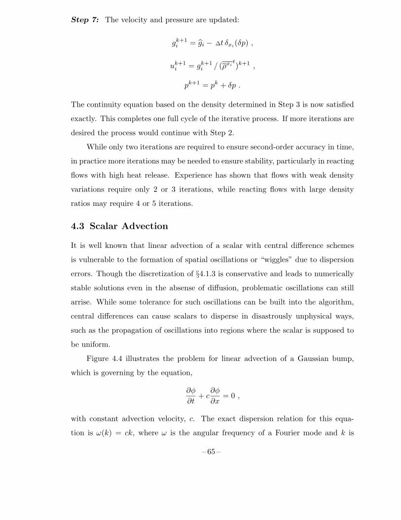
Step 7: The velocity and pressure are updated:

gk+1i = gi − ∆t δxi(δp) ,

uk+1i = gk+1i / (ρxit)k+1 ,

pk+1 = pk + δp .

The continuity equation based on the density determined in Step 3 is now satisfied

exactly. This completes one full cycle of the iterative process. If more iterations are

desired the process would continue with Step 2.

While only two iterations are required to ensure second-order accuracy in time,

in practice more iterations may be needed to ensure stability, particularly in reacting

flows with high heat release. Experience has shown that flows with weak density

variations require only 2 or 3 iterations, while reacting flows with large density

ratios may require 4 or 5 iterations.

4.3 Scalar Advection

It is well known that linear advection of a scalar with central difference schemes

is vulnerable to the formation of spatial oscillations or “wiggles” due to dispersion

errors. Though the discretization of §4.1.3 is conservative and leads to numerically

stable solutions even in the absense of diffusion, problematic oscillations can still

arrise. While some tolerance for such oscillations can be built into the algorithm,

central differences can cause scalars to disperse in disastrously unphysical ways,

such as the propagation of oscillations into regions where the scalar is supposed to

be uniform.

Figure 4.4 illustrates the problem for linear advection of a Gaussian bump,

which is governing by the equation,

∂φ

∂t+ c

∂φ

∂x= 0 ,

with constant advection velocity, c. The exact dispersion relation for this equa-

tion is ω(k) = ck, where ω is the angular frequency of a Fourier mode and k is

– 65 –

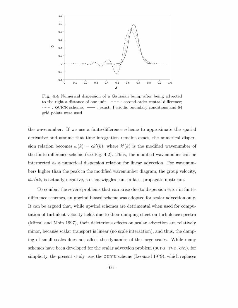
0 0.1 0.2 0.3 0.4 0.5 0.6 0.7 0.8 0.9 1.0-0.4

-0.2

0

0.2

0.4

0.6

0.8

1.0

1.2

�

�

Fig. 4.4 Numerical dispersion of a Gaussian bump after being advected

to the right a distance of one unit. : second-order central difference;

: quick scheme; : exact. Periodic boundary conditions and 64

grid points were used.

the wavenumber. If we use a finite-difference scheme to approximate the spatial

derivative and assume that time integration remains exact, the numerical disper-

sion relation becomes ω(k) = ck′(k), where k′(k) is the modified wavenumber of

the finite-difference scheme (see Fig. 4.2). Thus, the modified wavenumber can be

interpreted as a numerical dispersion relation for linear advection. For wavenum-

bers higher than the peak in the modified wavenumber diagram, the group velocity,

dω/dk, is actually negative, so that wiggles can, in fact, propagate upstream.

To combat the severe problems that can arise due to dispersion error in finite-

difference schemes, an upwind biased scheme was adopted for scalar advection only.

It can be argued that, while upwind schemes are detrimental when used for compu-

tation of turbulent velocity fields due to their damping effect on turbulence spectra

(Mittal and Moin 1997), their deleterious effects on scalar advection are relatively

minor, because scalar transport is linear (no scale interaction), and thus, the damp-

ing of small scales does not affect the dynamics of the large scales. While many

schemes have been developed for the scalar advection problem (supg, tvd, etc.), for

simplicity, the present study uses the quick scheme (Leonard 1979), which replaces

– 66 –

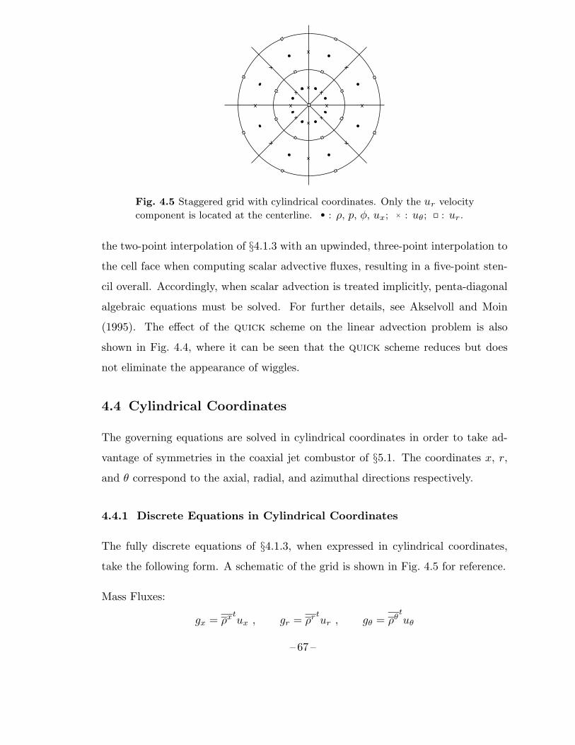
Fig. 4.5 Staggered grid with cylindrical coordinates. Only the ur velocitycomponent is located at the centerline. • : ρ, p, φ, ux; × : uθ; : ur.

the two-point interpolation of §4.1.3 with an upwinded, three-point interpolation to

the cell face when computing scalar advective fluxes, resulting in a five-point sten-

cil overall. Accordingly, when scalar advection is treated implicitly, penta-diagonal

algebraic equations must be solved. For further details, see Akselvoll and Moin

(1995). The effect of the quick scheme on the linear advection problem is also

shown in Fig. 4.4, where it can be seen that the quick scheme reduces but does

not eliminate the appearance of wiggles.

4.4 Cylindrical Coordinates

The governing equations are solved in cylindrical coordinates in order to take ad-

vantage of symmetries in the coaxial jet combustor of §5.1. The coordinates x, r,

and θ correspond to the axial, radial, and azimuthal directions respectively.

4.4.1 Discrete Equations in Cylindrical Coordinates

The fully discrete equations of §4.1.3, when expressed in cylindrical coordinates,

take the following form. A schematic of the grid is shown in Fig. 4.5 for reference.

Mass Fluxes:

gx = ρxtux , gr = ρr

tur , gθ = ρθ

tuθ

– 67 –

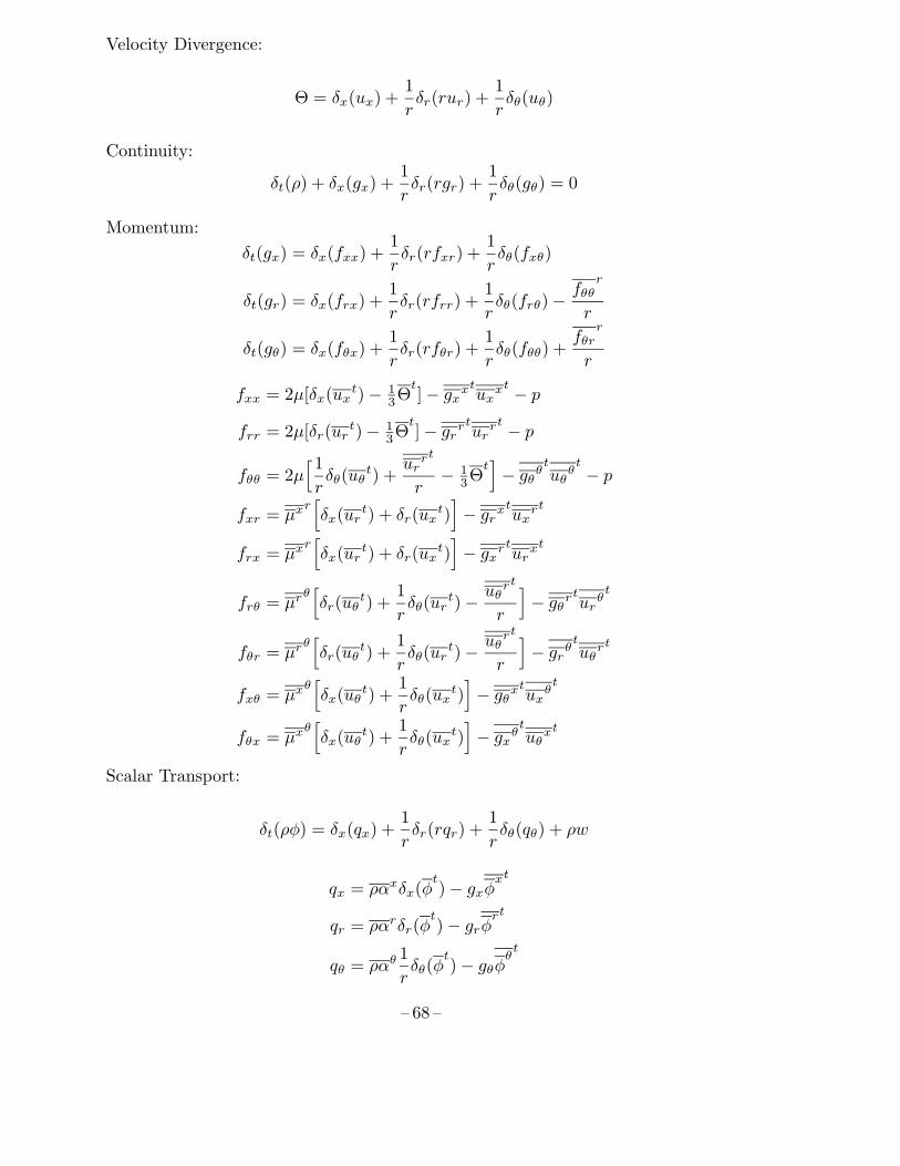
Velocity Divergence:

Θ = δx(ux) +1

rδr(rur) +

1

rδθ(uθ)

Continuity:

δt(ρ) + δx(gx) +1

rδr(rgr) +

1

rδθ(gθ) = 0

Momentum:

δt(gx) = δx(fxx) +1

rδr(rfxr) +

1

rδθ(fxθ)

δt(gr) = δx(frx) +1

rδr(rfrr) +

1

rδθ(frθ)−

fθθr

r

δt(gθ) = δx(fθx) +1

rδr(rfθr) +

1

rδθ(fθθ) +

fθrr

r

fxx = 2µ[δx(uxt)− 1

3Θt]− gxx

tux

xt − p

frr = 2µ[δr(urt)− 1

3Θt]− grr

tur

rt − p

fθθ = 2µ[1rδθ(uθ

t) +ur

rt

r− 13Θt]− gθθ

tuθ

θt− p

fxr = µxr[δx(ur

t) + δr(uxt)]− grx

tux

rt

frx = µxr[δx(ur

t) + δr(uxt)]− gxr

tur

xt

frθ = µrθ[δr(uθ

t) +1

rδθ(ur

t)− uθrt

r

]− gθr

tur

θt

fθr = µrθ[δr(uθ

t) +1

rδθ(ur

t)− uθrt

r

]− grθ

tuθ

rt

fxθ = µxθ[δx(uθ

t) +1

rδθ(ux

t)]− gθx

tux

θt

fθx = µxθ[δx(uθ

t) +1

rδθ(ux

t)]− gxθ

tuθ

xt

Scalar Transport:

δt(ρφ) = δx(qx) +1

rδr(rqr) +

1

rδθ(qθ) + ρw

qx = ραxδx(φt)− gxφ

xt

qr = ραrδr(φt)− grφ

rt

qθ = ραθ1

rδθ(φ

t)− gθφ

θt

– 68 –

Note that the pressure has been included in the momentum flux tensor, fij , rather

than written as a separate gradient term. In the radial momentum equation, pres-

sure contributes to both the radial flux and curvature terms, which combine to yield

an equivalent gradient term:

1

rδr(rp)−

pr

r= δr(p) .

4.4.2 Centerline Treatment

The centerline treatment used in this work differs considerably from that used by

Akselvoll and Moin (1995). Referring to Fig. 4.5, it is clear that all quantities

except ur are staggered in the radial direction with respect to the centerline (i.e.,

they are located at ∆r/2 from the centerline), while ur itself is collocated with the

centerline. An analysis of the discrete equations reveals that centerline conditions

are actually not needed for any of the variables, except for ur and fθr. Derivatives

of quantities that are staggered with respect to the centerline can be obtained by

differencing opposing values across the centerline, accounting for reversals in the

directions of the radial and azimuthal unit vectors through the centerline (Mohseni

and Colonius 2000). Centerline boundary conditions for ur and fθr are obtained by

averaging corresponding values across the centerline (Akselvoll and Moin 1995):

ur(r = 0, θ) = 12[ur(∆r, θ) + ur(∆r, θ + π)] . (4.26)

The approach is designed to allow radial flow communication through the centerline

without undue influence to or from points at neighboring θ locations. The angular

distribution of ur at the centerline does not necessarily conform to a single-valued

centerline velocity vector.

Grid quality was found to be important near the centerline in order to main-

tain solution stability. Although derivatives in radial direction are treated implicitly,

the scheme is in fact explicit in the radial direction at the centerline itself because

tri-diagonal equations are not coupled through the centerline. Thus, excessive re-

finement of the radial grid at the centerline can create stiffness. Also, excessive

– 69 –

grid stretching at the centerline was found to promote the formation of unstable

“wiggles” in the radial velocity component near the centerline.

4.4.3 Exact Representation of Uniform Flow

A uniform velocity field is represented in Cartesian coordinates as a vector with

constant components:

u = (U, V, W ) .

However, in cylindrical coordinates the components are not constant but vary with

θ:

u = (U, V cos θ +W sin θ, −V sin θ +W cos θ) .

When derivatives in the r and θ momentum equations are calculated using finite

differences, the discrete equations are not necessarily statisfied by the above uniform

flow solution. The discrepancies are particularly noticeable near the centerline,

where errors can be magnified by the 1/r factor.

It is usually desireable that a discrete representation of the governing equa-

tions satisfy exactly certain trivial flow situations, the case of uniform flow being

the simplest. This was achieved in the present formulation by “tweaking” cer-

tain differencing and interpolation operators in the discrete momentum equations

with multiplicative correction factors, so that a uniform flow satisfies the equations

exactly, while second-order accuracy is maintained. Specifically, derivatives and

interpolations in the θ direction are modified according to

δθ(u) −→sin(∆θ/2)

∆θ/2δθ(u) , uθ −→ cos(∆θ/2)uθ . (4.27)

The above modifications can be thought of as accounting for the finite angular

spacing of the computational grid. Note that as ∆θ → 0, the correction factors

approach unity.

4.5 Boundary Conditions

Staggered grids can be problematic when boundary conditions need to be applied,

because some of the variables may not be properly located with respect to the

– 70 –

�

�

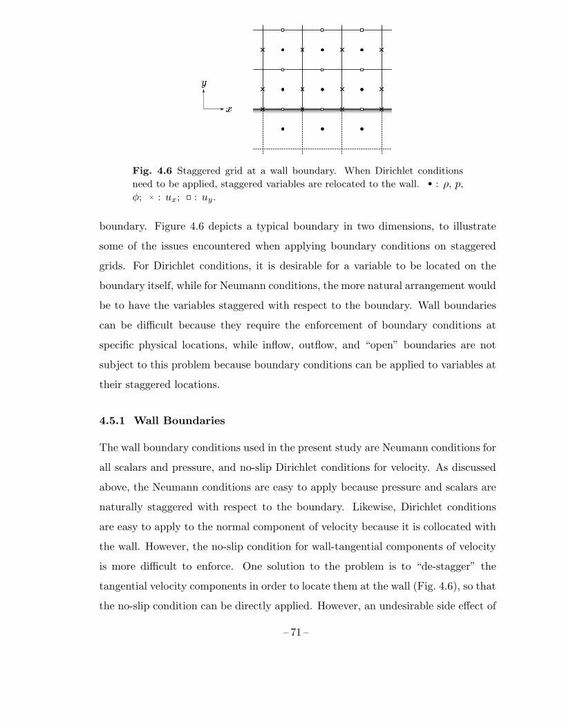
Fig. 4.6 Staggered grid at a wall boundary. When Dirichlet conditions

need to be applied, staggered variables are relocated to the wall. • : ρ, p,φ; × : ux; : uy.

boundary. Figure 4.6 depicts a typical boundary in two dimensions, to illustrate

some of the issues encountered when applying boundary conditions on staggered

grids. For Dirichlet conditions, it is desirable for a variable to be located on the

boundary itself, while for Neumann conditions, the more natural arrangement would

be to have the variables staggered with respect to the boundary. Wall boundaries

can be difficult because they require the enforcement of boundary conditions at

specific physical locations, while inflow, outflow, and “open” boundaries are not

subject to this problem because boundary conditions can be applied to variables at

their staggered locations.

4.5.1 Wall Boundaries

The wall boundary conditions used in the present study are Neumann conditions for

all scalars and pressure, and no-slip Dirichlet conditions for velocity. As discussed

above, the Neumann conditions are easy to apply because pressure and scalars are

naturally staggered with respect to the boundary. Likewise, Dirichlet conditions

are easy to apply to the normal component of velocity because it is collocated with

the wall. However, the no-slip condition for wall-tangential components of velocity

is more difficult to enforce. One solution to the problem is to “de-stagger” the

tangential velocity components in order to locate them at the wall (Fig. 4.6), so that

the no-slip condition can be directly applied. However, an undesirable side effect of

– 71 –

this grid redefinition is to create a discontinuity in the wall-normal grid spacing at

the boundary, which causes the wall-normal difference operator to become only first

order accurate. This has led other investigators (Caruso 1985; Akselvoll and Moin

1995) to consider three-point, one-sided difference operators for computing the wall

stress. However, giving special treatment to the numerical method on boundaries

was considered undesireable for code generality, and for simplicity, the wall stress

was computed using the standard two-point difference operator even though the

accuracy is degraded to first order.

4.5.2 Inflow Conditions

Turbulent inflow conditions for les must reflect the three-dimensional, unsteady

nature of turbulence. In principle, the computational domain should be extended

to include all the upstream geometry and flow conditioning devices (such as swirl

vanes) that may influence flow properties farther downstream. But because this is

usually not practical, approximate inflow conditions must be considered. In many

cases, the inflow condition is a developing turbulent duct flow that can be approxi-

mated as fully developed. The unsteady inflow conditions can then be generated by

simulating a spatially periodic section of the duct. Generalization of this approach

to generate swirling inflow conditions is discussed by Pierce and Moin (1998b).

In the present study, a separate inflow generation code was used to create

an “inflow database”. The inflow generator simulates a spatially periodic, fully

developed, parallel duct flow. Every few time steps, a cross section of velocity data

is saved to the inflow database, until sufficient inflow data have been accumulated to

provide converged turbulence statistics. In the main simulation, planes of velocity

data are read from the inflow database in succession and applied to the inflow

boundary. Linear interpolation in both space and time is performed when the

inflow database grid and time step do not exactly match the grid and time step of

the main simulation. If the end of the database is reached before the simulation

is completed, inflow sampling returns to the beginning of the database, thereby

recycling turbulent inflow conditions when necessary. This is not expected to cause

– 72 –

any problems when the database contains sufficient samples to produce converged

statistics and when the main simulation contains flow time scales longer than the

inflow recyling interval.

When the inflow conditions cannot be approximated as fully developed, their

specification becomes significantly more difficult. Usually, some specified mean ve-

locity or turbulence statistics profiles are known from an experiment or a Reynolds-

average calculation, and it is desired to have the same statistics profiles applied to

the inflow boundary of the les. However, as stated in the beginning of this section,

les requires instantaneous turbulence data, not merely their statistical properties.

Previous approaches to this problem (Le and Moin 1994; Akselvoll and Moin 1995)

involved the specification of statistically constrained random numbers at the inflow

boundary, which was followed by a development section that allowed the random

numbers to develop into realistic turbulence. Although random numbers are easy

to synthesize, they do not make a very attractive boundary condition because of

the need for a costly development section and because of the fact that initial ran-

dom numbers that are constrained to have the proper statistics do not necessarily

develop into turbulence having the desired statistics. In fact, extreme changes in

the flow are observed to occur within the first few grid points downstream of the

imposed boundary condition.

A more attractive approach is to generalize the “fully developed” approxima-

tion described above to include the larger class of parallel flows having arbitrarily

specified velocity statistics profiles. This type of flow is created by simulating a

spatially periodic, parallel duct flow and constraining it using a corrective “forc-

ing” technique. The resulting flow has the desired statistical properties, and it

provides realistic turbulence data that are in “equilibrium” with the specified mean

statistics. In the following, x is the streamwise coordinate direction, y and z are

cross-stream directions, and u(x, y, z, t) is the instantaneous streamwise velocity

component. Assume that a desired mean velocity profile, U(y, z), and fluctuation

intensity profile, U ′(y, z) are given. The forcing technique then proceeds as follows.

At each time step, the streamwise-averaged velocity, u(y, z, t), and fluctuation vari-

– 73 –

ance, u′2(y, z, t), are computed:

u(y, z, t) = 〈u(x, y, z, t)〉x ,

u′2(y, z, t) =⟨u(x, y, z, t)2

⟩x− u(y, z, t)2 .

Then, the instantaneous velocity field is rescaled and shifted so that is has the

specified mean and fluctuating velocity profiles:

u(x, y, z, t) −→ U ′(y, z)√u′2(y, z, t)

[u(x, y, z, t)− u(y, z, t)] + U(y, z) . (4.28)

This would be equivalent to adding an appropriately defined body force to the u-

component momentum equation. If only the mean velocity profile is constrained,

then (4.28) would be replaced by the simpler procedure,

u(x, y, z, t) −→ u(x, y, z, t)− u(y, z, t) + U(y, z) . (4.29)

The above approach appears to be an attractive alternative for generating real-

istic turbulent inflow conditions having specified mean statistical properties and

was considered in this study when fully developed conditions were deemed to be

inadequate.

4.5.3 Outflow Conditions

The convective condition is used for all “outflow” boundaries, which may also in-

clude “open” boundaries where the flow may actually enter the domain, as occurs

for example, when ambient fluid is entrained into a free jet. Mathematically, this

condition is written,∂φ

∂t+ c

∂φ

∂n= 0 , (4.30)

where φ is any scalar variable or velocity component, c is the convection velocity,

and n is the coordinate in the direction of the outward normal at the boundary.

In non-Cartesian coordinates, the normal component of velocity satisfies a slightly

modifed form of the convective condition to account for changes in flow area in

– 74 –

the direction normal to the boundary. Instead of ∂un/∂n, the corresponding term

from the continuity equation is used. For example, in cylindrical coordinates, the

convective condition for the radial component of velocity at a radially oriented

outflow boundary satisfies,

∂ur∂t

+ c1

r

∂rur∂r

= 0 . (4.31)

This ensures that the time-average of the ouflow mass flux is the same as the mass

flux at the first interior point away from the boundary.

Normal derivatives at the outflow boundary are evaluated using one-sided, first-

order differences, and the convection velocity is taken to be constant over the outflow

boundary. Flow structures that approach the boundary at speeds higher than c are

forced to slow and compress in a manner similar to a stagnation point, often with

the formation of unphysical “wiggles” that can propagate upstream (§4.3), whilestructures that move slower than c will be stretched and “pulled” out of the domain

without wiggle formation. If c is too large, however, the cfl restriction may limit

the time step, and in the limit c → ∞, the convective condition approaches a

Neumann condition. Based on these observations, a good choice for c will be just

large enough to prevent structures from stagnating at the boundary. Thus, c is

changed at each time step to equal the maximum outflow velocity over the outflow

boundary, c = max(un).

Global mass conservation is satisfied if the total outflow mass flux balances the

total inflow mass flux plus the net change in mass storage in the interior of the

domain. This is enforced at each time step by adding a corrective constant to the

outflow velocity (except at the walls in the boundary plane), to mimic the physical

response to a uniform pressure gradient at the outflow boundary. Thus, changes in

the inflow mass flow rate, as well as heat release fluctuations in the interior domain,

are balanced by adjustments to the outflow mass flow rate.

– 75 –

– 76 –

Chapter 5

APPLICATION TO ACOAXIAL JET COMBUSTOR

The models and numerical methods described in previous chapters were tested against ex-

perimental data for a methane fueled coaxial jet combustor. Simulations were performed

using all three chemistry models presented in §3.3 under otherwise identical conditions andwere compared with each other and with experimental data. In addition, the importance

of accounting for differential diffusion effects with the progress-variable approach was ex-

amined. The results show that only the progress-variable approach predicts a lifted flame

and gives satisfactory agreement with experimental data in the region close to the inlet. If

unity Lewis numbers are assumed and differential diffusion is neglected, the results for the

progress-variable approach are significantly worse when compared to experimental data in

the region close to the inlet, where the interaction between chemical kinetics and mixing

is important.

5.1 Experimental Configuration

The experimental study used for the validation of the simulation methodology was

the coaxial jet combustor configuration of Owen et al. (1976). This experiment

was chosen for its relatively simple geometry and boundary conditions yet complex

flow patterns resembling those in a gas turbine combustor, and for the availability of

detailed measurements that map the species, temperature, and velocity fields within

the combustor. The experimental study consisted of eight test cases conducted

under various operating conditions and geometric modifications. The particular

case used for the present validation, referred to as “Test 1” in the laboratory report

(Spadaccini et al. 1976), is depicted in Fig. 5.1.

The configuration had a relatively large diameter, low velocity central fuel

port, with higher velocity, nonswirling air in a surrounding annulus. The air was

preheated to 750K, and the combustor was pressurized to 3.8 atm. Porous-metal

discs were installed in the fuel injector and air entry section to provide uniform inlet

– 77 –

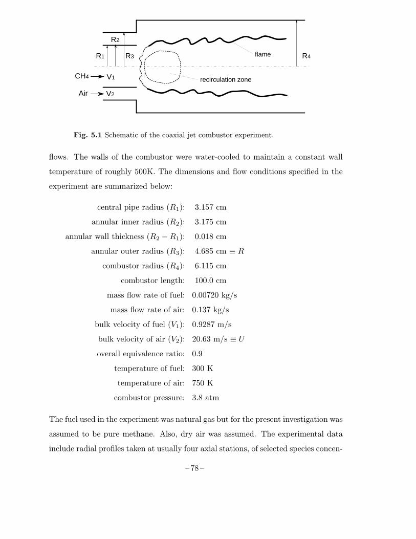
CH4

Air V2

V1

R4

recirculation zone

flameR1

R2

R3

Fig. 5.1 Schematic of the coaxial jet combustor experiment.

flows. The walls of the combustor were water-cooled to maintain a constant wall

temperature of roughly 500K. The dimensions and flow conditions specified in the

experiment are summarized below:

central pipe radius (R1): 3.157 cm

annular inner radius (R2): 3.175 cm

annular wall thickness (R2 −R1): 0.018 cm

annular outer radius (R3): 4.685 cm ≡ R

combustor radius (R4): 6.115 cm

combustor length: 100.0 cm

mass flow rate of fuel: 0.00720 kg/s

mass flow rate of air: 0.137 kg/s

bulk velocity of fuel (V1): 0.9287 m/s

bulk velocity of air (V2): 20.63 m/s ≡ U

overall equivalence ratio: 0.9

temperature of fuel: 300 K

temperature of air: 750 K

combustor pressure: 3.8 atm

The fuel used in the experiment was natural gas but for the present investigation was

assumed to be pure methane. Also, dry air was assumed. The experimental data

include radial profiles taken at usually four axial stations, of selected species concen-

– 78 –

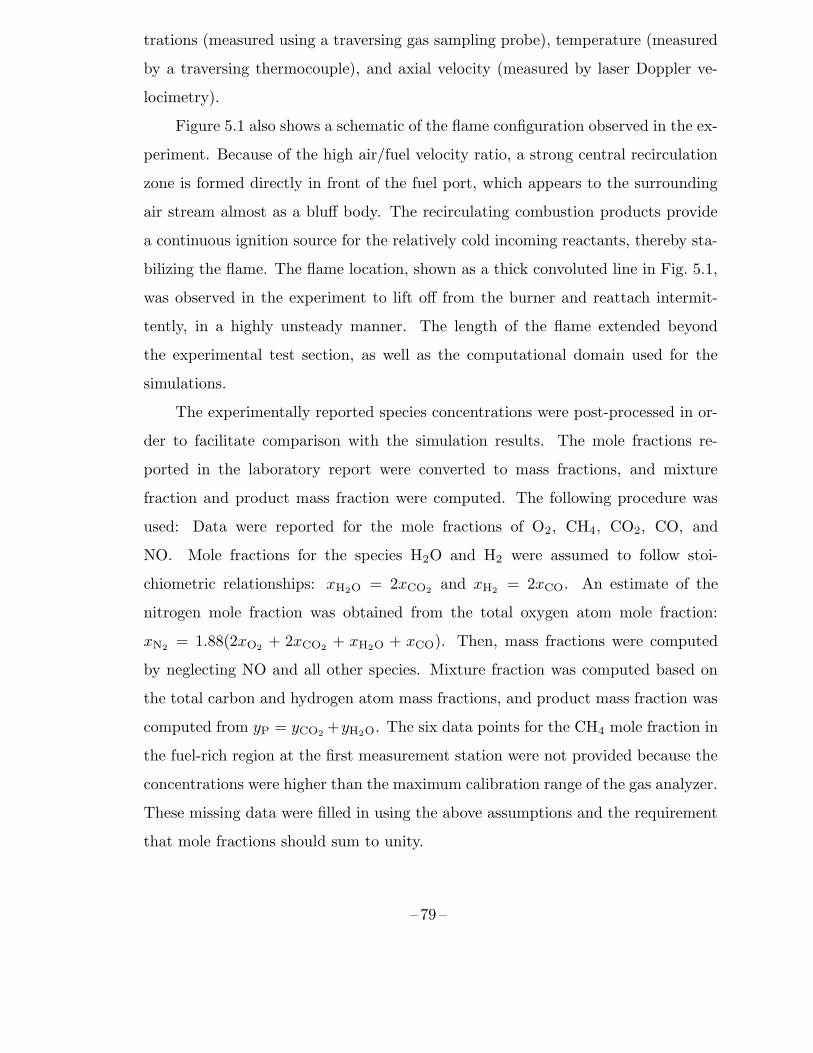
trations (measured using a traversing gas sampling probe), temperature (measured

by a traversing thermocouple), and axial velocity (measured by laser Doppler ve-

locimetry).

Figure 5.1 also shows a schematic of the flame configuration observed in the ex-

periment. Because of the high air/fuel velocity ratio, a strong central recirculation

zone is formed directly in front of the fuel port, which appears to the surrounding

air stream almost as a bluff body. The recirculating combustion products provide

a continuous ignition source for the relatively cold incoming reactants, thereby sta-

bilizing the flame. The flame location, shown as a thick convoluted line in Fig. 5.1,

was observed in the experiment to lift off from the burner and reattach intermit-

tently, in a highly unsteady manner. The length of the flame extended beyond

the experimental test section, as well as the computational domain used for the

simulations.

The experimentally reported species concentrations were post-processed in or-

der to facilitate comparison with the simulation results. The mole fractions re-

ported in the laboratory report were converted to mass fractions, and mixture

fraction and product mass fraction were computed. The following procedure was

used: Data were reported for the mole fractions of O2, CH4, CO2, CO, and

NO. Mole fractions for the species H2O and H2 were assumed to follow stoi-

chiometric relationships: xH2O = 2xCO2and xH2

= 2xCO. An estimate of the

nitrogen mole fraction was obtained from the total oxygen atom mole fraction:

xN2= 1.88(2xO2

+ 2xCO2+ xH2O + xCO). Then, mass fractions were computed

by neglecting NO and all other species. Mixture fraction was computed based on

the total carbon and hydrogen atom mass fractions, and product mass fraction was

computed from yP = yCO2+yH2O. The six data points for the CH4 mole fraction in

the fuel-rich region at the first measurement station were not provided because the

concentrations were higher than the maximum calibration range of the gas analyzer.

These missing data were filled in using the above assumptions and the requirement

that mole fractions should sum to unity.

– 79 –

5.2 Computational Setup

A picture of the grid used for all of the simulations is shown in Fig. 5.2. The

distribution of grid points was not determined by any systematic rules, but rather

by experience and trial-and-error, although general requirements are that the grid be

smooth and be refined near solid boundaries and in particular in the axial direction

at the jet orifice. The thinness of the annular wall separating fuel and air required

that especially fine radial resolution be used there. The size of the grid was 256×150× 64 points in the axial, radial, and azimuthal directions, respectively, and was

determined by cost considerations as the largest grid on which the simulations could

be completed in a reasonable amount of time.

Fig. 5.2 Schematic of the grid used for the simulations. Only half of the

points in the axial and radial directions are shown for clarity.

The simulations were computed using length (R), velocity (U), and time (R/U)

scales normalized by the injector radius (R ≡ R3) and the inlet bulk velocity of the

air (U ≡ V2). All simulation results are presented and compared with the experi-

mental data using these units. The computational domain started at a distance of

1R upstream of the combustor, where fully developed turbulent inflow conditions

were specified using the method of §4.5.2, even though the experimental inflow

conditions were probably not fully developed. The computational domain contin-

ued until a combustor length of 8R was reached, at which point convective outflow

boundary conditions (§4.5.3) were specified. All of the solid boundaries were as-

sumed to be adiabatic and impermeable, including the annular splitter plate, even

though the combustor walls in the experiment were isothermal.

– 80 –

To initialize a new simulation, the velocity and scalar fields are initially set

to zero everywhere. Pressure impulsively starts the flow as inlet conditions are

applied, initially producing a potential flow. The Reynolds number is temporarily

reduced for the first few time steps to avoid problems with initial sharp gradients.

A starting vortex forms at the jet orifice, convects downstream, and eventually

leaves the domain. Turbulence from the inlet gradually fills the domain, eventually

becoming fully developed. All future simulations of the same configuration, for

example after adjusting the grid or changing the chemistry model, are initialized

by interpolating previous fully-developed solutions. Fully developed incompressible

velocity and mixing fields are obtained before the chemistry model is turned on.

For the progress-variable approach (§3.3.4), the initial progress scalar field is set

to its maximum allowed value determined from fast chemistry, so that initially the

flame is fully ignited.

Solutions to the flamelet equations (3.35) were computed using gri-mech 3.0

and multicomponent mass diffusion, including Soret and Dufour effects for com-

pleteness. The parameter L0 in (3.39) was chosen to be 2 cm. Additional flamelet

libraries were computed using other mass diffusion models for the results of §5.3.2.For the progress-variable approach, product mass fraction (yP = yCO2

+ yH2O) was

chosen to serve as the progress variable. The log-normal distribution for dissipation

rate was used with the steady flamelet model. When the steady flamelet model

was used in the simulation, a type of feedback instability was observed: A sudden

increase in the dissipation rate can cause a sudden increase in density, which dur-

ing the following time step can cause the dissipation rate to increase even further.

Likewise, a sudden decrease in dissipation rate can cause the density to decrease,

further decreasing the dissipation rate at the next time level. In order to avoid the

instability, a time filtering was applied, in which the computed dissipation rate, χ,

was averaged with the dissipation rate computed at the previous time step (not the

previous average) before it was used to determine a new density field.

– 81 –

The computational time step was was selected by computing a generalized cfl

number,

CFL =u∆t

∆x+ν ∆t

∆x2, (5.1)

based only on axial convection and diffusion. Radial and azimuthal convection

and diffusion are not included in the cfl estimate because these terms are treated

implicitly. A time step of 0.005 R/U was used for all of the simulations and cor-

responded to a cfl number that varied within a range of about 0.5 – 1.0. For

the progress-variable approach, the maximum progress-variable reaction rate in the

flamelet library was sufficiently small that no stiffness was caused by the chemical

source term.

All of the statistical results obtained from the simulations are based on simple

averages of the resolved fields in time and in the azimuthal direction. No attempt

was made to account for subgrid contributions to the statistics or to account for

any effects due to the implicit Favre filtering described in §3.1. Because of the long

time scales present in the combustor, a large number of time steps was required to

integrate the flow long enough to obtain reasonably converged statistics. The total

time needed for initial flow development as well as statistical sampling was about

500 R/U time units or 100,000 time steps for each simulation. The simulations

were run on the ASCI Red platform (Sandia National Laboratory, Albuquerque,

New Mexico) using 512 processors, yielding a sustained aggregate performance of

10 Gflops, or about 3.7 seconds per time step. Thus, about 50,000 processor-hours

were used per simulation.

5.3 Results

A total of four large eddy simulations of the coaxial jet combustor described in §5.1were performed, each configured with exactly the same computational parameters,

but using a different chemistry model: (1) fast chemistry, (2) steady flamelets, (3)

progress-variable approach, and (4) progress-variable approach with unity Lewis

numbers. The first three simulations are compared in §5.3.1, where it is found that

both the fast chemistry and steady flamelet models fail to account for extinction

– 82 –

and flame lift-off close to the burner, while the progress-variable approach predicts

a lifted flame and obtains favorable agreement with the experimental data. The

third and fourth simulations are compared in §5.3.2 to demonstrate that inclusion

of differential diffusion effects is necessary to obtain good agreement with the ex-

perimental data.

5.3.1 Chemistry Model Comparison

In this section, results for the three chemistry models described in §3.3 are examined

and compared to each other and to experimental data. The most important ques-

tion to be answered is whether the simulation methodology is capable of accurately

capturing the gross characteristics and behavior of the flame, such as the rate of

product formation and heat release, flame lift-off, ignition, and extinction. Char-

acteristics that depend on the details of the combustion process, such as pollutant

formation, are not a target of the present effort. The primary quantities that are

used to examine the characteristics of each simulation are the mixture fraction (Z)

and product mass fraction (yP = yCO2+ yH2O).

Figure 5.3 compares instantaneous, planar snapshots of mixture fraction for

each of the chemistry models: (a) fast chemistry, (b) steady flamelet, and (c)

progress variable approach. Since the three simulations are configured identically

except for the chemistry model, and since mixture fraction is a conserved scalar,

which does not participate in chemical reactions, one might expect the mixture frac-

tion results for the three cases to be very similar. But scalar mixing can be strongly

influenced by heat release, which depends directly on the chemistry model. This is

because heat release causes flow dilatation to occur within the thin mixing layers

between fuel and oxidizer, thereby pushing apart fuel and oxidizer when they try to

mix. In general, the rate of mixing is found to decrease with higher rates of chemical

heat release, so that mixture fraction can be used as an indicator of whether the

location and rate of chemical reactions are accurately predicted by the chemistry

model. The effect of heat release on mixing is clearly visible when comparing the

mixing characteristics in the initial thin mixing layers just after the annular splitter

– 83 –

plate in Fig. 5.3(a,b), where mixing appears weak, and in Fig. 5.3(c), where small

rollers are visible. The general conclusion to be drawn from Fig. 5.3 is that, of

the three chemistry models tested, the fast chemistry model has the lowest rate

of mixing, the progress-variable approach has the highest, and the rate of mixing

with the steady flamelet model lies somewhere between the other two, all due to

the resulting heat release rate.

Corresponding pictures of product mass fraction are shown in Fig. 5.4. Flame

location is identified by the regions of highest product concentration, typically ap-

pearing as thin corrugated white lines. Both the fast chemistry and steady flamelet

models clearly have attached flames, while the progress variable approach shows a

much more complicated and asymmetric pattern: At the particular instant shown,

the flame is lifted on the upper side of the injector and is intermittently attached on

the lower side. This behavior is highly unsteady and must be viewed as an anima-

tion to be fully appreciated. Because of the extinction occurring on the upper side,

unburned reactants are able to penetrate into the interior of the flame as indicated

by the darker areas in the center of Fig. 5.4(c). The small amounts of product

visible in the inlet region of the fuel port are due to occasional recirculation of hot

products inside the inlet. In Fig. 5.4(a), the fast chemistry model always predicts

the theoretical maximum product mass fraction for the given mixture fraction. The

highest product mass fraction possible is approximately yP = 0.275 and occurs at

the stoichiometric mixture fraction, Zst = 0.0552, when all fuel and oxidizer have

been converted into product. In Fig. 5.4(b), the steady flamelet model predicts sig-

nificantly lower product mass fractions than the theoretical maximum. This is due

to the “quenching” effect that scalar dissipation rate has on diffusion flame struc-

ture. The steady flamelet model also shows numerous small-scale, wavy structures

throughout the central region. These variations should be considered unphysical

and a defect of the steady flamelet model, because they are due solely to local fluc-

tuations in dissipation rate in a region where there is mixing between product and

fuel but little or no reaction. In flamelet theory, it is the dissipation rate occurring

at the flame surface (the “stoichiometric” dissipation rate) that controls the flame

– 84 –

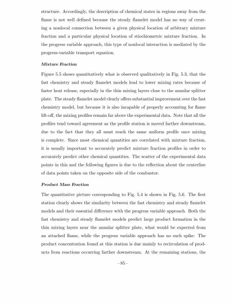
structure. Accordingly, the description of chemical states in regions away from the

flame is not well defined because the steady flamelet model has no way of creat-

ing a nonlocal connection between a given physical location of arbitrary mixture

fraction and a particular physical location of stiochiometric mixture fraction. In

the progress variable approach, this type of nonlocal interaction is mediated by the

progress-variable transport equation.

Mixture Fraction

Figure 5.5 shows quantitatively what is observed qualitatively in Fig. 5.3, that the

fast chemistry and steady flamelet models lead to lower mixing rates because of

faster heat release, especially in the thin mixing layers close to the annular splitter

plate. The steady flamelet model clearly offers substantial improvement over the fast

chemistry model, but because it is also incapable of properly accounting for flame

lift-off, the mixing profiles remain far above the experimental data. Note that all the

profiles tend toward agreement as the profile station is moved farther downstream,

due to the fact that they all must reach the same uniform profile once mixing

is complete. Since most chemical quantities are correlated with mixture fraction,

it is usually important to accurately predict mixture fraction profiles in order to

accurately predict other chemical quantities. The scatter of the experimental data

points in this and the following figures is due to the reflection about the centerline

of data points taken on the opposite side of the combustor.

Product Mass Fraction

The quantitative picture corresponding to Fig. 5.4 is shown in Fig. 5.6. The first

station clearly shows the similarity between the fast chemistry and steady flamelet

models and their essential difference with the progress variable approach. Both the

fast chemistry and steady flamelet models predict large product formation in the

thin mixing layers near the annular splitter plate, what would be expected from

an attached flame, while the progress variable approach has no such spike: The

product concentration found at this station is due mainly to recirculation of prod-

ucts from reactions occurring farther downstream. At the remaining stations, the

– 85 –

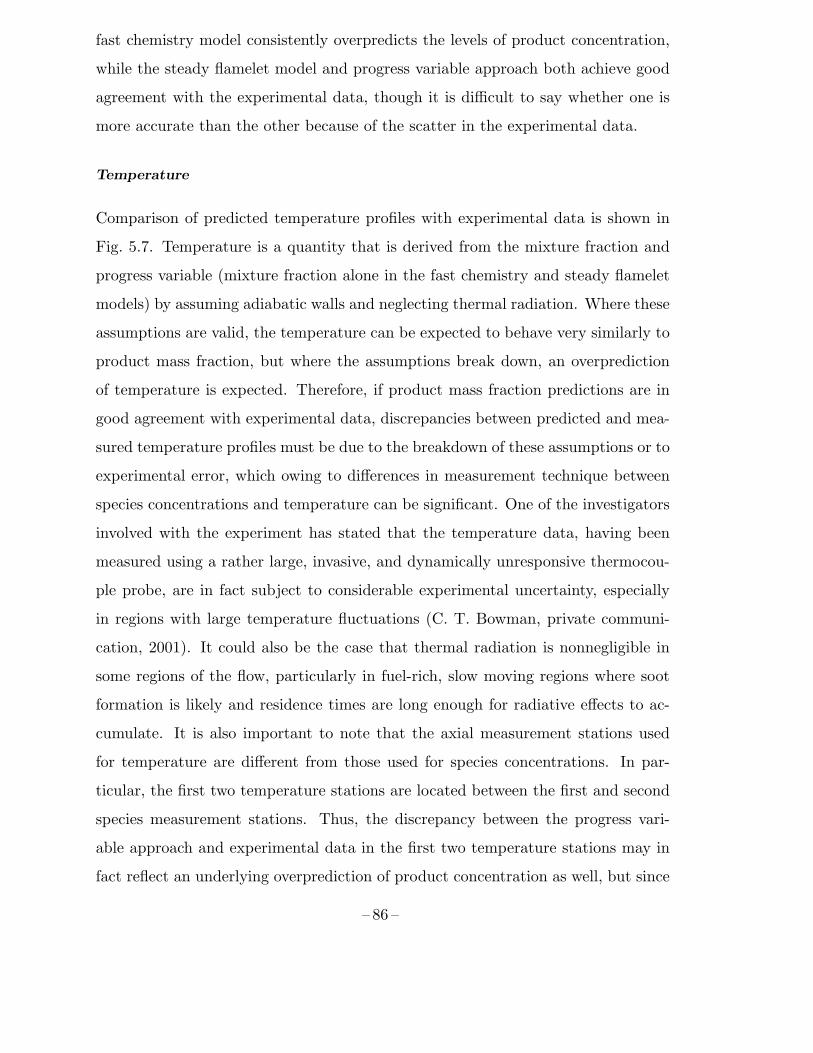
fast chemistry model consistently overpredicts the levels of product concentration,

while the steady flamelet model and progress variable approach both achieve good

agreement with the experimental data, though it is difficult to say whether one is

more accurate than the other because of the scatter in the experimental data.

Temperature

Comparison of predicted temperature profiles with experimental data is shown in

Fig. 5.7. Temperature is a quantity that is derived from the mixture fraction and

progress variable (mixture fraction alone in the fast chemistry and steady flamelet

models) by assuming adiabatic walls and neglecting thermal radiation. Where these

assumptions are valid, the temperature can be expected to behave very similarly to

product mass fraction, but where the assumptions break down, an overprediction

of temperature is expected. Therefore, if product mass fraction predictions are in

good agreement with experimental data, discrepancies between predicted and mea-

sured temperature profiles must be due to the breakdown of these assumptions or to

experimental error, which owing to differences in measurement technique between

species concentrations and temperature can be significant. One of the investigators

involved with the experiment has stated that the temperature data, having been

measured using a rather large, invasive, and dynamically unresponsive thermocou-

ple probe, are in fact subject to considerable experimental uncertainty, especially

in regions with large temperature fluctuations (C. T. Bowman, private communi-

cation, 2001). It could also be the case that thermal radiation is nonnegligible in

some regions of the flow, particularly in fuel-rich, slow moving regions where soot

formation is likely and residence times are long enough for radiative effects to ac-

cumulate. It is also important to note that the axial measurement stations used

for temperature are different from those used for species concentrations. In par-

ticular, the first two temperature stations are located between the first and second

species measurement stations. Thus, the discrepancy between the progress vari-

able approach and experimental data in the first two temperature stations may in

fact reflect an underlying overprediction of product concentration as well, but since

– 86 –

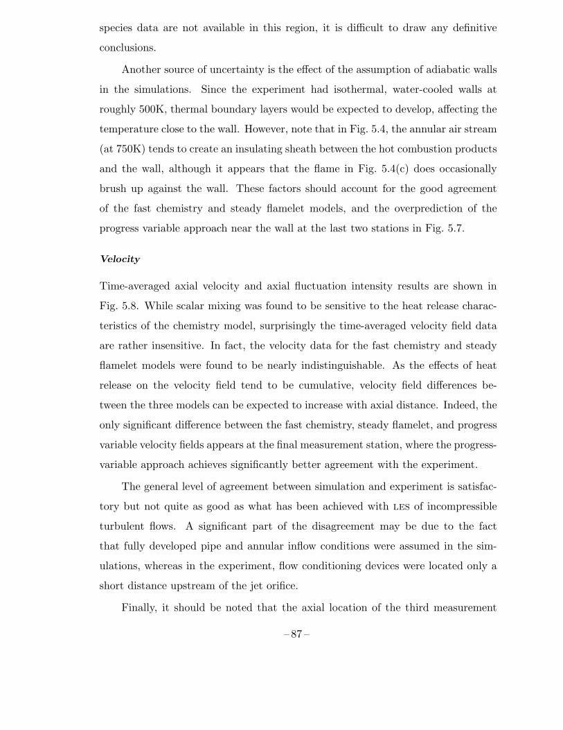
species data are not available in this region, it is difficult to draw any definitive

conclusions.

Another source of uncertainty is the effect of the assumption of adiabatic walls

in the simulations. Since the experiment had isothermal, water-cooled walls at

roughly 500K, thermal boundary layers would be expected to develop, affecting the

temperature close to the wall. However, note that in Fig. 5.4, the annular air stream

(at 750K) tends to create an insulating sheath between the hot combustion products

and the wall, although it appears that the flame in Fig. 5.4(c) does occasionally

brush up against the wall. These factors should account for the good agreement

of the fast chemistry and steady flamelet models, and the overprediction of the

progress variable approach near the wall at the last two stations in Fig. 5.7.

Velocity

Time-averaged axial velocity and axial fluctuation intensity results are shown in

Fig. 5.8. While scalar mixing was found to be sensitive to the heat release charac-

teristics of the chemistry model, surprisingly the time-averaged velocity field data

are rather insensitive. In fact, the velocity data for the fast chemistry and steady

flamelet models were found to be nearly indistinguishable. As the effects of heat

release on the velocity field tend to be cumulative, velocity field differences be-

tween the three models can be expected to increase with axial distance. Indeed, the

only significant difference between the fast chemistry, steady flamelet, and progress

variable velocity fields appears at the final measurement station, where the progress-

variable approach achieves significantly better agreement with the experiment.

The general level of agreement between simulation and experiment is satisfac-

tory but not quite as good as what has been achieved with les of incompressible

turbulent flows. A significant part of the disagreement may be due to the fact

that fully developed pipe and annular inflow conditions were assumed in the sim-

ulations, whereas in the experiment, flow conditioning devices were located only a

short distance upstream of the jet orifice.

Finally, it should be noted that the axial location of the third measurement

– 87 –

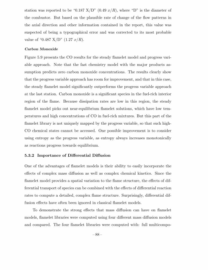
station was reported to be “0.187 X/D” (0.49 x/R), where “D” is the diameter of

the combustor. But based on the plausible rate of change of the flow patterns in

the axial direction and other information contained in the report, this value was

suspected of being a typographical error and was corrected to its most probable

value of “0.487 X/D” (1.27 x/R).

Carbon Monoxide

Figure 5.9 presents the CO results for the steady flamelet model and progress vari-

able approach. Note that the fast chemistry model with the major products as-

sumption predicts zero carbon monoxide concentrations. The results clearly show

that the progress variable approach has room for improvement, and that in this case,

the steady flamelet model significantly outperforms the progress variable approach

at the last station. Carbon monoxide is a significant species in the fuel-rich interior

region of the flame. Because dissipation rates are low in this region, the steady

flamelet model picks out near-equilibrium flamelet solutions, which have low tem-

peratures and high concentrations of CO in fuel-rich mixtures. But this part of the

flamelet library is not uniquely mapped by the progress variable, so that such high-

CO chemical states cannot be accessed. One possible improvement is to consider

using entropy as the progress variable, as entropy always increases monotonically

as reactions progress towards equilibrium.

5.3.2 Importance of Differential Diffusion

One of the advantages of flamelet models is their ability to easily incorporate the

effects of complex mass diffusion as well as complex chemical kinetics. Since the

flamelet model provides a spatial variation to the flame structure, the effects of dif-

ferential transport of species can be combined with the effects of differential reaction

rates to compute a detailed, complex flame structure. Surprisingly, differential dif-

fusion effects have often been ignored in classical flamelet models.

To demonstrate the strong effects that mass diffusion can have on flamelet

models, flamelet libraries were computed using four different mass diffusion models

and compared. The four flamelet libraries were computed with: full multicompo-

– 88 –

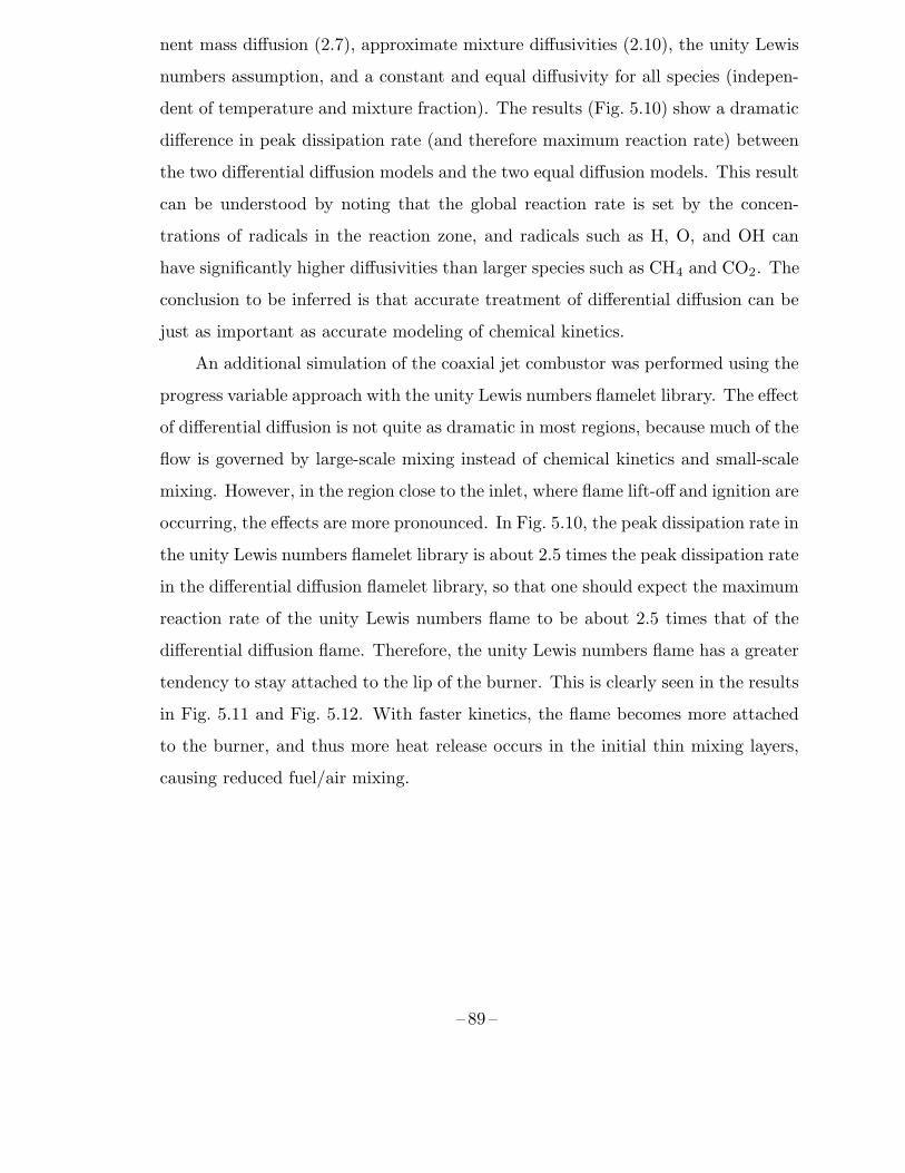
nent mass diffusion (2.7), approximate mixture diffusivities (2.10), the unity Lewis

numbers assumption, and a constant and equal diffusivity for all species (indepen-

dent of temperature and mixture fraction). The results (Fig. 5.10) show a dramatic

difference in peak dissipation rate (and therefore maximum reaction rate) between

the two differential diffusion models and the two equal diffusion models. This result

can be understood by noting that the global reaction rate is set by the concen-

trations of radicals in the reaction zone, and radicals such as H, O, and OH can

have significantly higher diffusivities than larger species such as CH4 and CO2. The

conclusion to be inferred is that accurate treatment of differential diffusion can be

just as important as accurate modeling of chemical kinetics.

An additional simulation of the coaxial jet combustor was performed using the

progress variable approach with the unity Lewis numbers flamelet library. The effect

of differential diffusion is not quite as dramatic in most regions, because much of the

flow is governed by large-scale mixing instead of chemical kinetics and small-scale

mixing. However, in the region close to the inlet, where flame lift-off and ignition are

occurring, the effects are more pronounced. In Fig. 5.10, the peak dissipation rate in

the unity Lewis numbers flamelet library is about 2.5 times the peak dissipation rate

in the differential diffusion flamelet library, so that one should expect the maximum

reaction rate of the unity Lewis numbers flame to be about 2.5 times that of the

differential diffusion flame. Therefore, the unity Lewis numbers flame has a greater

tendency to stay attached to the lip of the burner. This is clearly seen in the results

in Fig. 5.11 and Fig. 5.12. With faster kinetics, the flame becomes more attached

to the burner, and thus more heat release occurs in the initial thin mixing layers,

causing reduced fuel/air mixing.

– 89 –

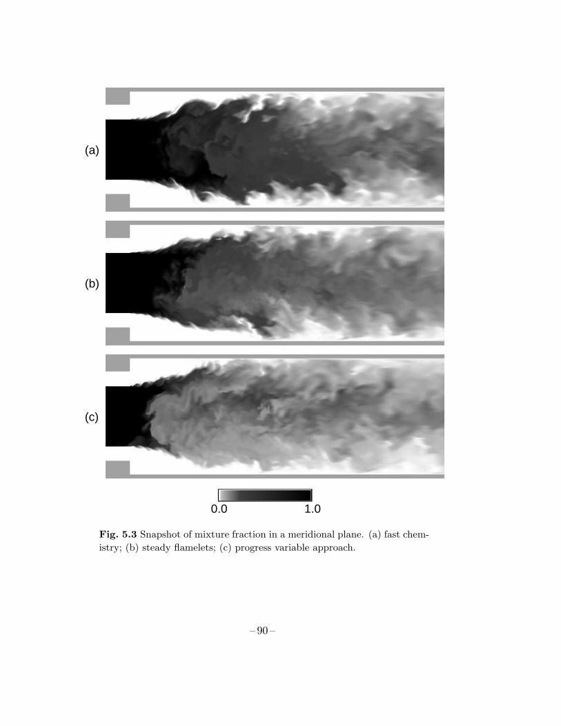
(a)

(b)

(c)

0.0 1.0

Fig. 5.3 Snapshot of mixture fraction in a meridional plane. (a) fast chem-

istry; (b) steady flamelets; (c) progress variable approach.

– 90 –

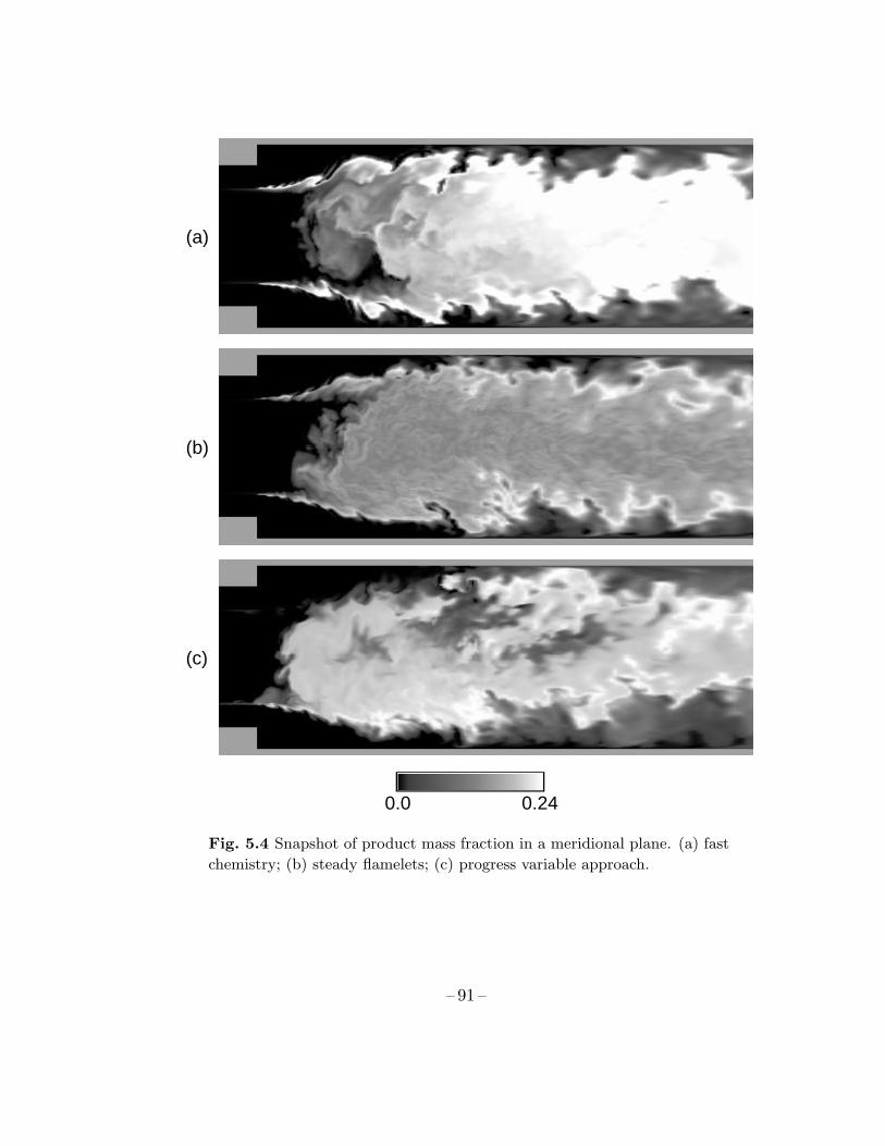
(a)

(b)

(c)

0.0 0.24

Fig. 5.4 Snapshot of product mass fraction in a meridional plane. (a) fast

chemistry; (b) steady flamelets; (c) progress variable approach.

– 91 –

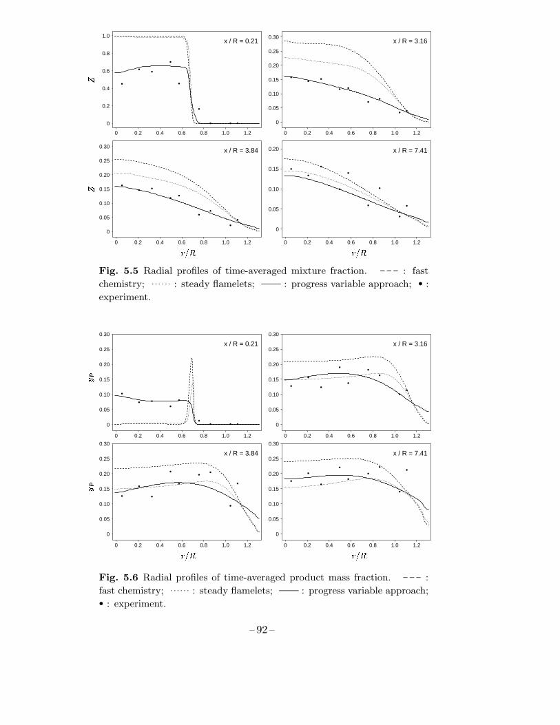
0 0.2 0.4 0.6 0.8 1.0 1.2

0

0.2

0.4

0.6

0.8

1.0

0 0.2 0.4 0.6 0.8 1.0 1.2

0

0.05

0.10

0.15

0.20

0.25

0.30

0 0.2 0.4 0.6 0.8 1.0 1.2

0

0.05

0.10

0.15

0.20

0.25

0.30

0 0.2 0.4 0.6 0.8 1.0 1.2

0

0.05

0.10

0.15

0.20

x / R = 0.21

����� �����

x / R = 3.16

x / R = 3.84 x / R = 7.41

�

Fig. 5.5 Radial profiles of time-averaged mixture fraction. : fast

chemistry; : steady flamelets; : progress variable approach; • :

experiment.

0 0.2 0.4 0.6 0.8 1.0 1.2

0

0.05

0.10

0.15

0.20

0.25

0.30

0 0.2 0.4 0.6 0.8 1.0 1.2

0

0.05

0.10

0.15

0.20

0.25

0.30

0 0.2 0.4 0.6 0.8 1.0 1.2

0

0.05

0.10

0.15

0.20

0.25

0.30

0 0.2 0.4 0.6 0.8 1.0 1.2

0

0.05

0.10

0.15

0.20

0.25

0.30

x / R = 0.21

���� ����

x / R = 3.16

x / R = 3.84 x / R = 7.41

� �

� �

Fig. 5.6 Radial profiles of time-averaged product mass fraction. :

fast chemistry; : steady flamelets; : progress variable approach;• : experiment.

– 92 –

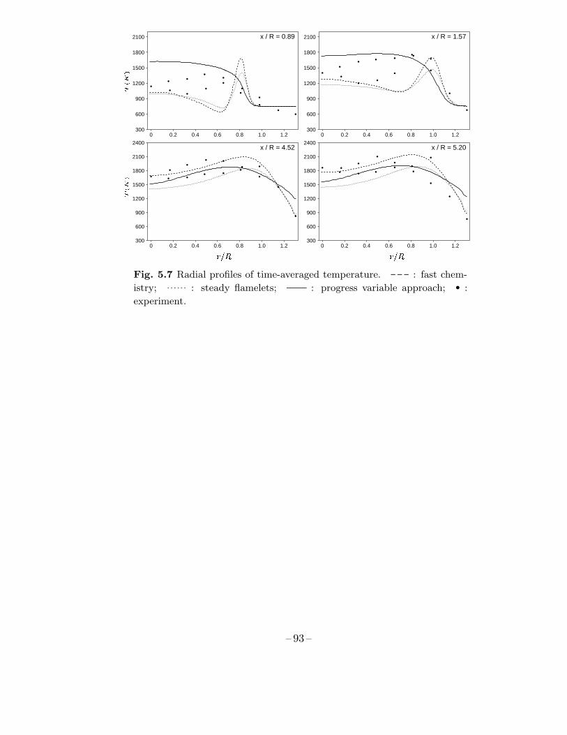
0 0.2 0.4 0.6 0.8 1.0 1.2 300

600

900

1200

1500

1800

2100

0 0.2 0.4 0.6 0.8 1.0 1.2 300

600

900

1200

1500

1800

2100

0 0.2 0.4 0.6 0.8 1.0 1.2 300

600

900

1200

1500

1800

2100

2400

0 0.2 0.4 0.6 0.8 1.0 1.2 300

600

900

1200

1500

1800

2100

2400

x / R = 0.89

����� �����

x / R = 1.57

x / R = 4.52 x / R = 5.20

� �

� ��

Fig. 5.7 Radial profiles of time-averaged temperature. : fast chem-

istry; : steady flamelets; : progress variable approach; • :

experiment.

– 93 –

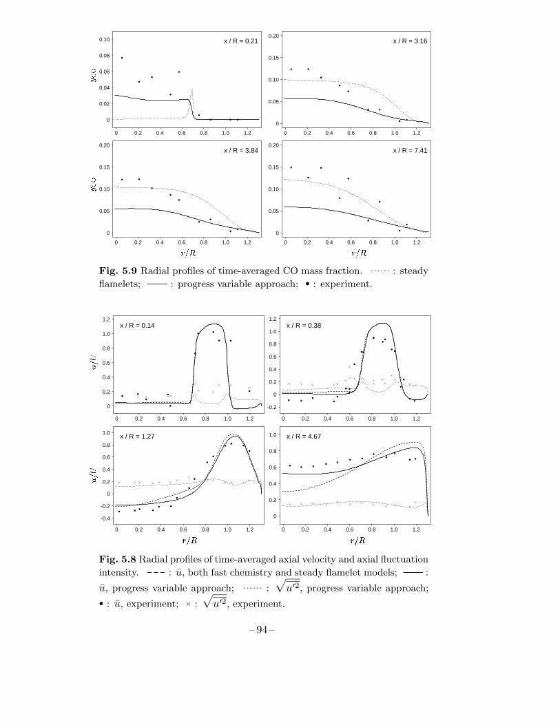
0 0.2 0.4 0.6 0.8 1.0 1.2

0

0.02

0.04

0.06

0.08

0.10

0 0.2 0.4 0.6 0.8 1.0 1.2

0

0.05

0.10

0.15

0.20

0 0.2 0.4 0.6 0.8 1.0 1.2

0

0.05

0.10

0.15

0.20

0 0.2 0.4 0.6 0.8 1.0 1.2

0

0.05

0.10

0.15

0.20

x / R = 0.21

����� �����

x / R = 3.16

x / R = 3.84 x / R = 7.41

�

� �

Fig. 5.9 Radial profiles of time-averaged CO mass fraction. : steady

flamelets; : progress variable approach; • : experiment.

0 0.2 0.4 0.6 0.8 1.0 1.2

0

0.2

0.4

0.6

0.8

1.0

1.2

0 0.2 0.4 0.6 0.8 1.0 1.2

-0.2

0

0.2

0.4

0.6

0.8

1.0

1.2

0 0.2 0.4 0.6 0.8 1.0 1.2

-0.4

-0.2

0

0.2

0.4

0.6

0.8

1.0

0 0.2 0.4 0.6 0.8 1.0 1.2

0

0.2

0.4

0.6

0.8

1.0

x / R = 0.14

����� �����

x / R = 0.38

x / R = 1.27 x / R = 4.67

�� �

�� �

Fig. 5.8 Radial profiles of time-averaged axial velocity and axial fluctuation

intensity. : u, both fast chemistry and steady flamelet models; :

u, progress variable approach; :√u′2, progress variable approach;

• : u, experiment; × :√u′2, experiment.

– 94 –

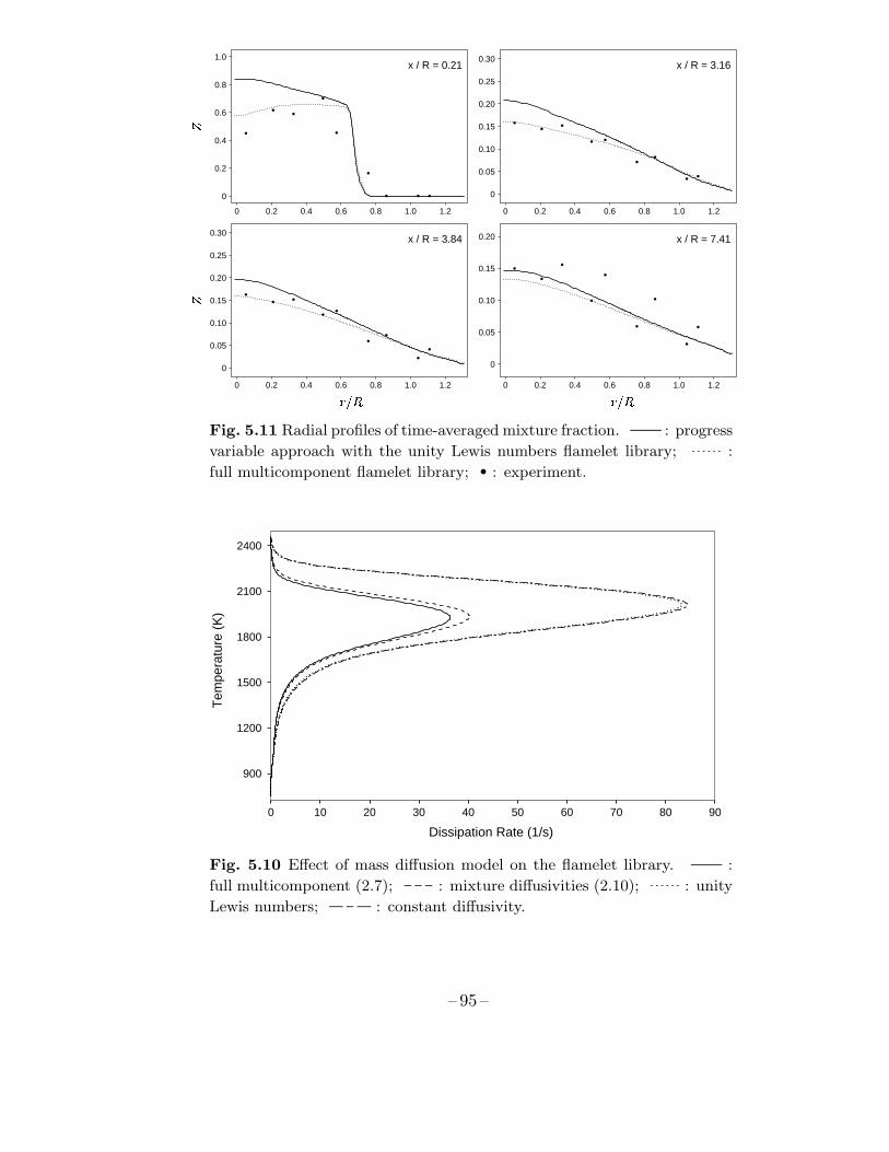
0 0.2 0.4 0.6 0.8 1.0 1.2

0

0.2

0.4

0.6

0.8

1.0

0 0.2 0.4 0.6 0.8 1.0 1.2

0

0.05

0.10

0.15

0.20

0.25

0.30

0 0.2 0.4 0.6 0.8 1.0 1.2

0

0.05

0.10

0.15

0.20

0.25

0.30

0 0.2 0.4 0.6 0.8 1.0 1.2

0

0.05

0.10

0.15

0.20

x / R = 0.21

����� �����

x / R = 3.16

x / R = 3.84 x / R = 7.41

�

Fig. 5.11 Radial profiles of time-averaged mixture fraction. : progress

variable approach with the unity Lewis numbers flamelet library; :

full multicomponent flamelet library; • : experiment.

Dissipation Rate (1/s)

Tem

pera

ture

(K

)

0 10 20 30 40 50 60 70 80 90

900

1200

1500

1800

2100

2400

Fig. 5.10 Effect of mass diffusion model on the flamelet library. :

full multicomponent (2.7); : mixture diffusivities (2.10); : unity

Lewis numbers; : constant diffusivity.

– 95 –

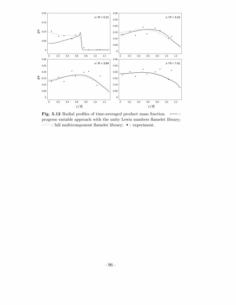
0 0.2 0.4 0.6 0.8 1.0 1.2

0

0.05

0.10

0.15

0.20

0 0.2 0.4 0.6 0.8 1.0 1.2

0

0.05

0.10

0.15

0.20

0.25

0.30

0 0.2 0.4 0.6 0.8 1.0 1.2

0

0.05

0.10

0.15

0.20

0.25

0.30

0 0.2 0.4 0.6 0.8 1.0 1.2

0

0.05

0.10

0.15

0.20

0.25

0.30

x / R = 0.21

����� �����

x / R = 3.16

x / R = 3.84 x / R = 7.41

�

�

Fig. 5.12 Radial profiles of time-averaged product mass fraction. :

progress variable approach with the unity Lewis numbers flamelet library;

: full multicomponent flamelet library; • : experiment.

– 96 –

Chapter 6

CONCLUSIONS ANDFUTURE DIRECTIONS

6.1 Conclusions

Large eddy simulation was shown to be a promising technique for prediction of com-

plex turbulent reacting flows. In the present work, a new algorithm was developed

for large eddy simulation of variable density reacting flows in simple combustor con-

figurations. Particular attention was given to both the primary conservation (mass,

momentum, scalar) and secondary conservation (kinetic energy, scalar “energy”)

properties of the method. The algorithm uses the primitive variables, which are

staggered in both space and time.

Motivated by the inability of existing chemistry models to predict lifted diffu-

sion flames, such as those occurring in gas turbine combustors, a new two-scalar

approach involving mixture fraction and a reaction progress variable was developed.

This is combined with a steady flamelet model that incorporates detailed chemical

kinetics and multicomponent mass diffusion.

The calculations were compared with detailed experimental data from the

United Technologies Research Center. Excellent agreement was obtained between

computations and the experiment in both the mean and fluctuating velocity profiles,

mean mixture fraction profiles, and mean product concentration. This agreement is

particularly significant because no adjustable parameters were available for tuning,

owing to the use of the dynamic procedure in the parameterization of turbulence.

Three chemistry models were tested in the present study: fast chemistry, steady

flamelet, and the progress-variable approach. The results show that the progress-

variable approach significantly outperforms both the fast chemistry and steady

– 97 –

flamelet models with only a marginal increase in computational cost. The progress-

variable approach appears to be an effective method for capturing basic realistic

flame behavior such as flame lift-off. However, the present formulation cannot ac-

curately predict details of the combustion process such as pollutant formation and

thermal radiation, and thus, future improvements will be necessary.

The present study has also shown that the inclusion of differential diffusion

effects is crucial, at least at the subgrid-scale level, for the prediction of the dynamics

of the near-field, where chemical kinetics and transport of radicals, which have a

broad range of diffusivities, are important.

6.2 Recommendations for Future Work

While the progress-variable approach presented in this study adds much capabil-

ity to the steady flamelet model, it is by no means a complete combustion model,

but rather a first step towards a more general approach. In its present form, the

progress-variable approach cannot account for convective heat transfer to bound-

aries, effects of radiation, premixed flame fronts, slow chemical processes such as

those involved in pollutant formation, and instabilities due to acoustic interactions.

The progress-variable approach can be extended to account for heat transfer to

boundaries by solving an additional transport equation for the total enthalpy, along

with the mixture fraction and progress variable. Total enthalpy would then become

an additional parameter in the flamelet chemistry tables. In this way, the effects

of the isothermal wall boundary conditions that were present in the experiment of

Owen et al. could be accounted for. A first step to account for radiation and soot

formation is to incorporate them directly into the calculation of the flamelet library.

A radiative loss term could also be added to the enthalpy transport equation.

An improvement in the choice of progress variable should also be considered.

The best candidate would be the entropy, because it is guaranteed to vary mono-

tonically with reaction progress and it should provide a better parameterization of

slowly evolving, near-equilibrium chemical states. However, entropy is governed by

a significantly more complicated equation than product mass fraction and includes

– 98 –

source terms for both mixing and chemical reaction.

To better model the formation of pollutants, the addition of secondary progress

variables, having significantly slower time scales than the primary progress variable,

should be considered. This may require further development of the chemical tab-

ulation procedures for the efficient calculation, storage, and retrieval of chemical

states.

The assumed pdf for the progress variable used in the present study does

not account for the effects of subgrid fluctuations is scalar dissipation rate or for

reaction front propagation in premixed and partially premixed combustion. Future

improvements to the this model should include both the effects of dissipation rate

and the chemical source term on the assumed shape of the pdf.

The numerical scheme for variable-density flows presented here can be extended

to include compressibility effects to account for low Mach number acoustics using a

Helmholtz equation for pressure. The special feature of this extension is that acous-

tic waves relevant to combustion instabilities can be accounted for at a considerable

savings in computer resources.

– 99 –

– 100 –

REFERENCES

Akselvoll, K. & Moin, P. (1995) “Large-eddy simulation of turbulent confined

coannular jets and turbulent flow over a backward facing step” Mech. Eng.

Dept. Report TF-63, Stanford University.

Akselvoll, K. & Moin, P. (1996) “Large-eddy simulation of turbulent confined

coannular jets” J. Fluid Mech. 315, 387–411.

Bird, R. B., Stewart, W. E., & Lightfoot, E. N (1960) Transport Phenom-

ena, John Wiley and Sons, New York.

Bushe, W. K. & Steiner, H. (1999) “Conditional moment closure for large eddy

simulation of nonpremixed turbulent reacting flows” Phys. Fluids 11, 1896–

1906.

Calhoon, W. H. & Menon, S. (1996) “Subgrid Modeling for Reacting Large

Eddy Simulations” AIAA Paper 96-0516.

Carati, D. & Eijnden, E. V. (1997) “On the self-similarity assumption in dy-

namic models for large eddy simulations” Phys. Fluids 9, 2165–2167.

Caruso, S. C. (1985) “Adaptive grid techniques for elliptic fluid-flow problems”

Ph.D. Thesis, Mech. Eng. Dept., Stanford University.

Colucci, P. J., Jaberi, F. A., Givi, P. & Pope, S. B. (1998) “Filtered density

function for large eddy simulation of turbulent reacting flows” Phys. Fluids 10,

499–515.

Cook, A. W. (1997) “Determination of the constant coefficient in scale similarity

models of turbulence” Phys. Fluids 9, 1485–1487.

Cook, A. W. & Riley, J. J. (1994) “A subgrid model for equilibrium chemistry

in turbulent flows” Phys. Fluids 6, 2868–2870.

Cook, A. W., Riley, J. J. & Kosaly, G. (1997) “A Laminar Flamelet Approach

to Subgrid-Scale Chemistry in Turbulent Flows” Combust. Flame 109, 332–

341.

Cuenot, B., Egolfopoulos, F. N. & Poinsot, T. (2000) “An unsteady laminar

flamelet model for non-premixed combustion” Combust. Theory Modelling 4,

– 101 –

77–97.

DesJardin, P. E. & Frankel, S. H. (1998) “Large eddy simulation of a tur-

bulent nonpremixed reacting jet: Application and assessment of subgrid-scale

combustion models” Phys. Fluids 10, 2298–2314.

Frankel, S. H., Adumitroaie, V., Madnia, C. K. & Givi, P. (1993) “Large

eddy simulation of turbulent reacting flows by assumed PDF methods” in En-

gineering Applications of Large Eddy Simulations, S. A. Ragab & U. Piomelli

(eds.), 81–101, ASME.

Gao, F. & O’Brien, E. E. (1993) “A large-eddy simulation scheme for turbulent

reacting flows” Phys. Fluids A 5, 1282–1284.

Germano, M., Piomelli, U., Moin, P. & Cabot, W. H. (1991) “A dynamic

subgrid-scale eddy viscosity model” Phys. Fluids A 3, 1760–1765.

Ghosal, S., Lund, T. S., Moin, P. & Akselvoll, K. (1995) “A dynamic lo-

calization model for large-eddy simulation of turbulent flows” J. Fluid Mech.

286, 229–255.

Ghosal, S. & Moin, P. (1995) “The Basic Equations for the Large Eddy Simula-

tion of Turbulent Flows in Complex Geometry” J. Comput. Phys. 118, 24–37.

Girimaji, S. S. & Zhou Y. (1996) “Analysis and modeling of subgrid scalar mixing

using numerical data” Phys. Fluids 8, 1224–1236.

Harlow, F. H. & Welch, J. E. (1965) “Numerial Calculation of Time-Dependent

Viscous Incompressible Flow of Fluid with Free Surface” Phys. Fluids 8, 2182–

2189.

Jaberi, F. A. & James, S. (1998) “A dynamic similarity model for large eddy

simulation of turbulent combustion” Phys. Fluids 10, 1775–1777.

Jaberi, F. A., Colucci, P. J., James, S., Givi, P. & Pope, S. B. (1999)

“Filtered mass density function for large-eddy simulation of turbulent reacting

flows” J. Fluid Mech. 401, 85–121.

Jimenez, J., Linan, A., Rogers, M. M. & Higuera, F. J. (1997) “A priori

testing of subgrid models for chemically reacting non-premixed turbulent shear

flows” J. Fluid Mech. 349, 149–171.

– 102 –

Johnson, B. V. & Bennett, J. C. (1981) “Mass and Momentum Turbulent

Transport Experiments with Confined Coaxial Jets” NASA CR-165574.

Johnson, B. V. and Bennett J. C. (1984) “Statistical Characteristics of Ve-

locity, Concentration, Mass Transport, and Momentum Transport for Coaxial

Jet Mixing in a Confined Duct” J. of Eng. for Gas Turbines and Power 106,

121–127.

Kerstein, A. R. (1992a) “Linear-eddy modeling of turbulent transport. Part 4.

Structure of diffusion flames” Combust. Sci. Tech. 81, 75–96.

Kerstein, A. R. (1992b) “Linear-eddy modeling of turbulent transport. Part 7.

Finite-rate chemistry and multi-stream mixing” J. Fluid Mech. 240, 289–313.

Klimenko, A. Y. & Bilger, R. W. (1999) “Conditional moment closure for

turbulent combustion” Prog. Energy Combust. Sci. 25, 595.

Le, H. & Moin, P. (1994) “Direct numerical simulation of turbulent flow over a

backward-facing step” Mech. Eng. Dept. Report TF-58, Stanford University.

Legier, J. P., Poinsot, T. & Veynante, D. (2000) “Dynamically thickened

flame LES model for premixed and non-premixed turbulent combustion” Pro-

ceedings of the 2000 CTR Summer Program, 157–168, Center for Turbulence

Research, NASA-Ames/Stanford University.

Leonard, B. P. (1979) “A stable and accurate convective modelling procedure

based on quadratic upstream interpolation” Comput. Meth. in Applied Mech.

and Eng. 19, 59–98.

Lesieur, M. & Metais, O. (1996) “New trends in large-eddy simulations of tur-

bulence” Ann. Rev. Fluid Mech. 28, 45–82.

Lilly, D. K. (1992) “A proposed modification of the Germano subgrid-scale closure

method” Phys. Fluids A 4, 633–635.

McMurtry, P. A., Menon, S. & Kerstein, A. R. (1993) “Linear eddy modeling

of turbulent combustion” Energy Fuels 7, 817–826.

Mittal, R. & Moin, P. (1997) “Suitability of upwind-biased finite difference

schemes for large-eddy simulation of turbulent flows” AIAA J. 35, 1415–1417.

Moin, P., Squires, K., Cabot, W. & Lee, S. (1991) “A dynamic subgrid-scale

– 103 –

model for compressible turbulence and scalar transport” Phys. Fluids A 3,

2746–2757.

Moin, P. (1997) “Progress in Large Eddy Simulation of Turbulent Flows” AIAA

Paper 97-0749.

Moin, P. (2001) Fundamentals of Engineering Numerical Analysis, Cambridge Uni-

versity Press.

Morinishi, Y., Lund, T. S., Vasilyev, O. V. & Moin, P. (1998) “Fully Con-

servative Higher Order Finite Difference Schemes for Incompressible Flow” J.

Comput. Phys. 143, 90–124.

Mohseni, K. & Colonius, T. (2000) “Numerical treatment of polar coordinate

singularities” J. Comput. Phys. 157, 787–795.

Muller, C. M., Breitbach, H. & Peters, N. (1994) “Partially premixed tur-

bulent flame propagation in jet flames” Proc. Combust. Inst. 25, 1099–1106.

Nicoud, F. (2000) “Conservative high-order finite-difference schemes for low-Mach

number flows” J. Comput. Phys. 158, 71–97.

Owen, F. K., Spadaccini, L. J. & Bowman, C. T. (1976) “Pollutant formation

and energy release in confined turbulent diffusion flames” Proc. Combust. Inst.

16, 105–117.

Peters, N. (1983) “Local Quenching Due to Flame Stretch and Non-Premixed

Turbulent Combustion” Combust. Sci. Tech. 30, 1–17.

Peters, N. (1984) “Laminar diffusion flamelet models in non-premixed turbulent

combustion” Prog. Energy Combust. Sci. 10, 319–339.

Peters, N. (1986) “Laminar flamelet concepts in turbulent combustion” Proc.

Combust. Inst. 21, 1231–1250.

Peters, N. (2000) Turbulent Combustion, Cambridge University Press.

Piacsek, S. A. & Williams, G. P. (1970) “Conservation Properties of Convection

Difference Schemes” J. Comput. Phys. 6, 392–405.

Pierce, C. D. & Moin, P. (1998a) “Large Eddy Simulation of a Confined Coaxial

Jet with Swirl and Heat Release” AIAA Paper 98-2892.

Pierce, C. D. & Moin, P. (1998b) “Method for Generating Equilibrium Swirling

– 104 –

Inflow Conditions” AIAA J. 36, 1325–1327.

Pierce, C. D. & Moin, P. (1998c) “A dynamic model for subgrid-scale variance

and dissipation rate of a conserved scalar” Phys. Fluids 10, 3041–3044.

Pitsch, H. & Peters, N. (1998) “A Consistent Flamelet Formulation for Non-

Premixed Combustion Considering Differential Diffusion Effects” Combust.

Flame 114, 26–40.

Pitsch, H. (2000) “Unsteady Flamelet Modeling of Differential Diffusion in Tur-

bulent Jet Diffusion Flames” Combust. Flame 123, 358–374.

Pitsch, H. & Steiner, H. (2000) “Large-eddy simulation of a turbulent piloted

methane/air diffusion flame (Sandia flame D)” Phys. Fluids 12, 2541–2554.

Pope, S. B. (1985) “PDF Methods for Turbulent Reactive Flows” Prog. Energy

Combust. Sci. 11, 119–192.

Pope, S. B. (1990) “Computations of turbulent combustion: Progress and chal-

lenges” Proc. Combust. Inst. 23, 591–612.

Reveillon, J. & Vervisch, L. (1998) “Subgrid-Scale Turbulent Micromixing:

Dynamic Approach” AIAA J. 36, 336–341.

Reynolds, W. C. (1986) “The element potential method for chemical equilibrium

analysis: implementation in the interactive program STANJAN” Mech. Eng.

Dept. Report, Stanford University.

Roback, R. & Johnson, B. V. (1983) “Mass and Momentum Turbulent Trans-

port Experiments with Confined Swirling Coaxial Jets” NASA CR-168252.

Sipperley, C. M., Huh, J. Y., Edwards, C. F. & Bowman, C. T. (1999)

“Experimental validation studies for large-eddy simulation of a gas turbine

main burner” CTR Annual Research Briefs, Center for Turbulence Research,

NASA Ames/Stanford University.

Spadaccini, L. J., Owen, F. K. & Bowman, C. T. (1976) “Influence of Aero-

dynamic Phenomena on Pollutant Formation in Combustion (Phase I. Gaseous

Fuels)” U.S. Environmental Protection Agency Report EPA-600/2-76-247a.

Steiner, H. & Bushe, W. K. (2001) “Large eddy simulation of a turbulent re-

acting jet with conditional source-term estimation” Phys. Fluids 13, 754–769.

– 105 –

Vasilyev, O. V., Lund, T. S. & Moin, P. (1998) “A General Class of Commu-

tative Filters for LES in Complex Geometries” J. Comput. Phys. 146, 82–104.

Vervisch, L. & Trouve, A. (1998) “LES modeling for lifted turbulent jet flames”

Proceedings of the 2000 CTR Summer Program, 83–100, Center for Turbulence

Research, NASA-Ames/Stanford University.

Wall, C., Boersma, B. J. & Moin, P. (2000) “An evaluation of the assumed beta

probability density function subgrid-scale model for large eddy simulation of

nonpremixed, turbulent combustion with heat release” Phys. Fluids 12, 2522–

2529.

Williams, F. A. (1985) Combustion Theory, 2nd ed., Addison-Wesley.

– 106 –