Dissertation

Essays on Choice under Uncertainty

zur Erlangung des akademischen Grades

doctor rerum politicarum

(Doktor der Wirtschaftswissenschaft)

eingereicht an der Wirtschaftswissenschaftlichen Fakultät

der Humboldt-Universität zu Berlin

von

Tobias Schmidt

Präsident der Humboldt-Universitätzu Berlin:

Dekan der Wirtschaftswissenschaftli-chen Fakultät:

Prof. Dr. Jan-Hendrik Olbertz Prof. Dr. Christian D. Schade

Gutachter:Prof. Georg Weizsäcker, Ph.D. PD Dr. Yves Breitmoser

Tag des Kolloqiums:30.06.2016

Essays on Choice under Uncertainty

Tobias Schmidt

21. April 2016

Acknowledgements

I am deeply indebted to a number of people and institutions for helping to makethis dissertation what it is.

First among them is my supervisor and co-author Georg Weizsäcker. Georg notonly gave me the freedom to pursue whatever ideas struck my fancy but also helpedme in every way imaginable to pursue them. He was there with advice when thoseideas developed in ways I had not anticipated or when I ran into problems. Hedissuaded me from pursuing some of my weaker ideas but did not hesitate to throwhis weight even behind ideas he must have known were risky or unpopular. He wasa source of guidance throughout the years, in matters of behavioral economics, thedesign of laboratory experiments and academic research more generally.

I have also had the great fortune of getting to collaborate with a number ofexceptional people on joint research projects, two of which have turned into Chap-ters 2 and 3 of this dissertation: Steffen Huck, with whom Georg and I collaboratedon the series of experiments that make up Chapter 2 and whose wide-ranging in-terests have been a constant source of inspiration. Charlie Sprenger, whom I metafter a seminar talk in Berlin and who invited me to spend two months at Stanford,a time during which parts of Chapter 3, in collaboration with James Andreoni,were written.

Then there is the wider group of people who provided the intellectual fermentfrom which this thesis draws.

Paul Viefers has been a long-time colleague and close friend. Paul was willingto listen to my ideas at a stage when calling them half-baked would have beencomplimentary, is one of the most able econometricians I know and a man with ataste and view of the world most similar to mine.

Yves Breitmoser taught me to take the task of confronting theory with data

iii

iv

seriously and often challenged me to look at issues through a different lens.I wrote this dissertation while a member of DIW Berlin’s Graduate Center, a

graduate program that was in its infancy when I arrived at DIW and which hassince developed nicely under the leadership of Georg Meran, Georg Weizsäckerand, most recently, Helmut Lütkepohl. It was the Graduate Center where I metmany of the people that have become good friends: Alexandra Avdeenko, JulianBaumann, Lilli Bügelmayer, Ludwig Ensthaler, Nils Saniter, Christoph GrosseSteffen, Jan Marcus, Sören Radde and Lilo Wagner.

For much of my tenure at DIW I was part of the Competition and Consumersdepartment. Special thanks go to the department head Pio Baake.

I owe a debt of gratitude to the Berlin Behavioral Economics community. Thisgroup, too, was in its infancy when I arrived in Berlin but has since become one ofthe largest groups of behavioral and experimental economists in Europe, if not theworld. Through its members and the regular series of seminars and workshops Iwas exposed to cutting-edge research on a staggering variety of topics. I would liketo thank Jana Friedrichsen, Paul Heidhues, Tobias Königs and Dorothea Kübler inparticular for the many discussions, and for guidance and support over the years.

I thank the European Research Council (Starting Grant 263412) for financialsupport.

Lastly, I am grateful for my family and my closest friends, Sebastian Königs andChico Blasques, who have stood by me over the years and, in a very real way, havemade me who I am.

Introduction

Mathematical theories of choice under risk and uncertainty are the bedrock onwhich modern economics is built. Almost all matters that economists concernthemselves with involve some element of uncertainty: The value of a good is seldomknown at the time of purchase and the consequences of activities as diverse asbuying stocks, going to college, choosing an occupation, getting married, havingchildren, smoking or exercising, taking out a life insurance policy or saving forretirement are either not known or unknowable when the decision is made. Atthe heart of any model of these subjects is a model of how people behave underuncertainty; how they perceive it, what their attitude towards it is and how thetwo jointly determine decisions.

Von Neumann and Morgenstern (1947) introduced expected utility theory, thefirst fully formalized theory of choice under risk, in their Theory of Games andEconomic Behavior.1 According to expected utility people make decisions as ifassigning values — “utilities” — to outcomes, weighting each utility by the ob-jectively given probability with which the outcome will occur and then choosingwhichever option gives them the highest weighted, expected utility. Von Neumannand Morgenstern thought of objectively given probabilities that were common toeveryone as a crutch and less than a decade later Savage (1954) demonstrated thatthis crutch was unnecessary. Von Neumann and Morgenstern’s theory could begeneralized so that every person was free to hold their own, subjective belief and,importantly, that under certain assumptions both people’s subjective beliefs andthe utilities they attach to different consequences can be inferred from the choicesthey make.

1 Though this was the first complete formal treatment of expected utility, precursors can befound in Daniel Bernoulli’s analysis of the St. Petersburg paradox in 1738 (Bernoulli, 1954).

v

vi

Expected utility — in both its objective and subjective version — quickly be-came the workhorse model of human decision making in modern economics andstill holds that status today. But almost immediately after its introduction it cameunder scrutiny for behavioral assumptions that were obviously at variance with theway people actually behaved. In the seven decades since the publication of TheTheory of Games and Economic Behavior expected utility has gone through sev-eral iterations and restatements and has been generalized in many directions inresponse to these critiques.

In expected utility the likelihoods with which consequences will materialize areeither objectively given or subjective judgments of the decision maker but are thenconsistently applied to evaluate all options. Some of the generalizations of expectedutility break with this consistency requirement. In (cumulative) prospect theory(Kahneman & Tversky, 1979; Tversky & Kahneman, 1992), for example, decisionmakers may distort the probability of an outcome depending on the rank of theconsequence in the gamble and even depending on whether the consequences isseen as a gain or loss relative to a reference point. The salience theory of Bordalo,Gennaioli, and Shleifer (2012) instead posits that some consequences “jump out” atdecision makers and therefore carry outsized weight in their decision-making pro-cess. Lastly, theories of ambiguity aversion like those of Schmeidler (1989), Gilboaand Schmeidler (1989) or Klibanoff, Marinacci, and Mukerji (2005) posit that thereis a fundamental difference between making decisions in situations in which prob-abilities are known and those in which they are not and that this gives rise toextremely cautious behavior that (subjective) expected utility cannot accommo-date. Other theories of choice under risk and uncertainty retain the evaluation ofoptions using a consistent probability measure but instead evaluate consequencesdifferently. In Loomes and Sugden’s (1982) regret theory, for examples the con-sequences of a gamble are evaluated not in isolation but relative to the otherconsequences that could have materialized: Gaining $100 may not be quite ashappy an occasion if an alternative option would have yielded even more.

While few of the stones from which expected utility is built have been leftunturned, almost all mathematical theories of choice under risk and uncertaintyhave retained one of expected utility’s core ideas: In all theories, options areevaluated by a functional that has expected utility form, however unusual either

vii

the utility function or the probability measure may sometimes appear to be. Peoplechoose among the alternatives by enumerating the possible consequences, makingjudgments about the likelihoods with which the consequences will occur, assigningto each consequence a subjective value and then assigning to the overall optiona value that is a sum of the value of the consequences, each weighted by somefunction of its likelihood. Common to all theories is therefore a separation of thetotal value of an option that drives choice into the utilities of its constituent partsand decision weights tied to beliefs about the likelihood with which those partswill materialize.

The three chapters of this dissertation shine a spotlight on models of choice underuncertainty in this tradition from three different directions. All three chapters areempirical, designed to either study how the theoretical constructs of utility andbeliefs can be measured, which of the many theories describes choices best andwhat explanatory power the theories hold.

Risk Aversion

Chapter 1 takes beliefs as a given and concerns itself with measuring and estimatingthe curvature of the utility function, which drives aversion to risk in expectedutility. The chapter is a re-analysis of Harrison, List, and Towe’s (2007) “NaturallyOccurring Preferences and Exogenous Laboratory Experiments: A Case Study ofRisk Aversion,” a paper that investigates the sensitivity of experimental proceduresfor eliciting people’s risk preferences to a number of auxiliary assumptions.

In risk preference elicitations it is commonly assumed that subjects will behavethe same in the elicitation task — a task that is fashioned to be a close empiricalanalogue to a theoretical construct, potentially at the cost of artifice — as theywould in the real-life situations that are of primary interest to economists. More-over, it is assumed that both wealth held outside the lab and risks faced outsideof the lab (“background risk”) play no role in determining the choices made insidethe lab. Both assumptions had always seemed questionable on theoretical grounds(see Gollier & Pratt, 1996; Rabin, 2000; Safra & Segal, 2008). Harrison et al. usean artefactual field experiment (Harrisson & List, 2004) to test these assumptionsempirically.

viii

The authors recruit numismatists to participate in one of three different elicita-tion tasks: All three tasks are multiple price list tasks à la Holt and Laury (2002),in which participants face a series of lottery choices. The three tasks differ in thenature of the prizes of the lotteries. The first task is an original Holt and Laurytask in which all prizes are monetary. In the second task the monetary prizes arereplaced by antique coins in different, known conditions. The authors view theselotteries over coins with which numismatists are intimately familiar as less artifi-cial and abstract than the lotteries over different amounts of money. In the thirdtask, finally, the prizes are the same coins as in the second but with the certificatesattesting to the coins’ condition removed. In this treatment subjects therefore hadto rely on their own expertise to assess the coins’ quality and must have felt atleast some uncertainty about the true value of the prizes, an additional risk thatwould remain even after the lottery had played out and which is mathematicallyequivalent to adding background risk.

Harrison et al. find that varying the artificiality of the experimental task has nostatistically significant effect on measured risk preferences nor do subjects behaveas if they integrated any of the wealth they hold outside of the lab. Exogenouslyvarying the amount of background risk, however, appears to have an enormousinfluence on measured risk aversion: Being exposed to an additional risk makessubjects much more risk averse.

At the heart of Harrison et al. and at the heart of the re-analysis in Chapter 1is a measurement issue. The textbook image of choice under risk is a neat one:every person has a utility function, uses this utility function to assign values toprizes and then integrates these values using the given probability measure. He orshe does this without fault and whatever option yields the highest expected utilityis chosen consistently. Experimental data do not, unfortunately, always conformto this textbook picture. Instead, when asked to make multiple choices, it is oftenimpossible to reconcile all choices with a single utility function. In the analysisof choice data one therefore frequently resorts to stochastic choice models, whichallow for non-systematic, random deviations from the “structural” drivers of choice(for an excellent survey of such models, see Wilcox, 2008).2

2 Some have argued that some classic behavioral “anomalies” could be the result of stochasticchoice, i.e. while they may appear to be systematic deviations from rationality they may, in

ix

The re-analysis shows that the conclusion that subjects become more risk aversein the face of higher background risk is not robust. It is instead the result of choicedata that, for many subjects, could not have been generated by deterministic utilitymaximization and an econometric model that takes the way in which choices departfrom deterministic utility maximization to be evidence of extreme risk aversion.Moreover, the sign, magnitude and statistical significance of the estimated effectof exposing subjects to less artificial prizes is highly dependent on the way onecontrols for individual heterogeneity in preferences.

Choices in Harrison et al.’s experiment are extremely noisy. One of the choicesthat subjects in all treatments are presented with, for example, is a “sanity check”,a choice between $200 and $350, both paid with certainty. For any subject whovalues money this should be an easy choice. Yet, 47% of the subjects who facethis choice choose the lower $200. Overall, a full 65% of subjects make choicesthat violate first-order stochastic dominance and are therefore inconsistent withmaximizing expected utility deterministically whatever their utility function. Inthe treatment that identifies the effect of exposing subjects to background risk,choices are particularly noisy. In this treatments subjects appear to be choosingbetween any pair of options put before them entirely at random.

On this data Harrison et al. estimate a “Fechner” stochastic choice model3 totest whether their experimental treatments have any effect on the amount of riskaversion subjects display. As the Chapter shows, this stochastic choice model isproblematic given the extent to which experimental responses depart from deter-ministic expected utility maximization. Perhaps surprisingly, there are two waysin which the Fechner model can accommodate choices that are completely unsys-tematic. The first and obvious way is by choosing a choice error so large thatany systematic preference is completely drowned out by noise. The second is by

fact, be entirely unsystematic (see e.g. Butler & Loomes, 2007; Collins & James, 2015; Hey& Orme, 1994). Because it creates choices that violate classical postulates like transitivityor monotonicity stochasticity is usually regarded as a mistake. More recently, however, someauthors have argued either that there is a higher form of rationality to stochastic choice —choice being stochastic mainly when consequences are of very similar value and when it maynot be worth figuring out which option is truly better — or even that there are situations inwhich people have a strict preference for randomization (see e.g. Agranov & Ortoleva, 2015;Dwenger, Kübler, & Weizsäcker, 2014)

3 So named because its origins are widely attributed to early work in psychophysics (Fechner,Adler, Howes, & Boring, 1966)

x

assuming extremely large risk aversion. As is by now well known (Wilcox, 2011),in the Fechner model higher risk aversion is mechanically linked to noisier choices.Asymptotically, both choice errors and high risk aversion imply completely ran-dom choice and identical distributions for the data, at which point the model isno longer identified. Chapter 1 shows that depending on the exact specificationthe data in the background risk treatment are either close to or squarely in thisasymptotic case, the reason for the noise being reflected in a high coefficient ofrelative risk aversion rather than in choice errors being that Harrison et al. do notallow the choice error to differ between treatments.

The extremely noisy data also makes HLT’s models numerically unstable andother results highly dependent on model specification. The effect of manipulatingthe artificiality of the task, negative and not statistically significantly differentfrom zero in the original paper, is statistically significantly positive in other spec-ifications.

Subjective Beliefs

While Chapter 1 takes the utility function as its main object of interest, Chapter 2,based on work with Georg Weizsäcker and Steffen Huck, puts its emphasis onthe second component of the expected utility functional: beliefs. The chapterexplores the role of subjective beliefs about stock market returns for stock marketinvestment behavior in a representative sample of the German population.

Taking its cue from Savage (1954) most of economics takes data on choices asits empirical primitive. The beliefs that underly these choices, in contrast, areimposed by assumption. Following a seminal paper by Muth (1961) agents areoften assumed to hold “rational expectations”, beliefs that are objectively correct,at least on average. The reasons for assuming that beliefs are objectively correctare less than compelling and making the assumption regardless may lead to biasedtests of other aspects of the theory. As an example, a person assumed to holdrational expectations about stock market returns may appear to be extremely,implausibly risk averse, this being the classical equity premium puzzle result ofMehra and Prescott (1985). But the equity premium would be less of a puzzle ifpeople thought equity returns to be lower or to be more variable than asset pricing

xi

models show them to be.4 As pointed out by Manski (2004), rational expectationsare an identifying assumption without which central parameters of interest are notidentified. Following Manski a rapidly growing literature has pursued a differentstrategy to achieve identification: by not only gathering data about people’s choicesbut also asking them for their subjective beliefs.

One way to read Chapter 2 is as probing the properties of the subjective beliefspeople report when asked. In particular, the Chapter asks what relationship thesereported beliefs bear to the subjective beliefs of SEU. The latter are not beliefsin the common sense meaning of that word but are instead beliefs derived fromchoice, indeed the beliefs that rationalize choice. Though it may be tempting totake it as a given that the two beliefs are identical, the chapter actually tests thisempirically. This test goes further than existing literature, which has found thatreported beliefs are predictive of behavior — people who expect the stock marketto do better than others tend to hold more stock (see e.g. Dominitz & Manski,2011; Hurd et al., 2011; Kézdi & Willis, 2009) — but has also uncovered limits tothe consistency between beliefs and behavior (see e.g. Merkle & Weber, 2014) and,importantly, has largely neglected issues of causality, i.e. whether people wouldhold more stock if they believed stock market returns to be more favorable.

The standard portfolio choice problem, a decision task in which a fixed sum ofmoney is to be distributed over two investment vehicles, a risk-free asset that paysa certain rate of return and a risky asset whose return is stochastic, serves as theframework for a series of experiments that explore the determinants of real-worldinvestment behavior. In the main experiment subjects in Germany are given e 25and confronted with the choice between a German government bond and an assetwhose return is tied to historic returns on Germany’s blue chip stock market indexDAX. An exogenous shifter whose sign and magnitude is known to subjects at thetime of investment is added to a return randomly chosen from the year-on-yearreturns on the DAX over the last 60 years.

The experiment then asks subjects to split the e 25 with which they are en-

4 The empirical evidence on whether beliefs are biased in ways that could explain the equitypremium is mixed. Some surveys (Dominitz & Manski, 2011; Hurd, van Rooij, & Winter,2011; Kézdi & Willis, 2009) find return expectations which are downward biased, others findbias in the opposite direction (Dominitz & Manski, 2011). The survey used in Chapter 2 findsbeliefs to be a fairly accurate reflection of the historical distribution of returns.

xii

dowed between these two assets and elicits the beliefs that should, under expectedutility and more general models, be major determinants of the investment decision.Subjects are asked for their subjective beliefs about the returns on the risky assetthey have before them. Using a question format due to Delavande and Rohwedder(2008) and further developed by Delavande, Giné, and McKenzie (2011) we elicitthe entire subjective belief distribution.

It’s the degree to which beliefs explain investments that is one of the mainquestions the experiment seeks to answer. Moreover, the study probes the extentto which subjects’ beliefs and their investment choices respond to the return shifter.Do subjects offered an investment in a risky asset whose returns are more favorablealso expect it to be more favorable? Do they invest more? Lastly, do subjects actsimilarly in the lab experiment as they do in real life?

The experiment was run with two groups of people: A representative sampleof about 700 German households which answered the 2012 survey of the Innova-tion Sample of the German Socioeconomic Panel, and a group of 198 students atTechnical University Berlin.

There are both similarities and differences between these two samples: In bothsamples return expectations are positively correlated with the amount of moneyallocated to the risky asset. In the SOEP sample, where information about partic-ipants’ real-life investments are known, there is also a strong relationship betweenchoices in the portfolio choice experiment and stock market participation: Thelarger the share of his or her endowment invested in the risky asset, the morelikely a participant is to own stocks. Indeed, this “equity share” appears to be anextremely potent predictor of stock holding even after controlling for a numberof other determinants that can be found in the literature — gender, age, educa-tion, household size, employment status, financial literacy, wealth and income —while, surprisingly, both beliefs and a measure of risk aversion do little to explainparticipation.

What is particularly interesting, however, are the responses to being treatedwith different return shifters. In the SOEP sample neither beliefs nor investmentsrespond in any way to the treatment: No matter whether the risky asset pays apast DAX return, a past DAX return minus ten percentage points or a past DAXreturn plus ten percentage points, on average participants have identical beliefs

xiii

about returns and allocate the same share of their endowment to the risky asset.Not so in the student sample. Here, too, beliefs do not respond to treatment.Investments, however, do change in the expected direction.

As an explanation for this surprising finding the paper offers a behavioral ex-planation that departs from subjective expected utility’s assumption that optionswhich are payoff-equivalent must be treated identically. In subjective expectedutility all that is decision-relevant are the distributions over final outcomes of theavailable options. The paper shows that while changes to the excess return of anasset should lead to the same change in investments no matter whether the changecomes about because the expected return on the safe asset changes or whether theexpected return on the risky asset changes, this may not, in fact, be true.

What the Chapter posits instead is that people find it easier to mentally processchanges to an object that is relatively simple rather than one that is complex, assuggested by previous lab and field evidence (see e.g Abeler & Jäger, 2015; Chetty,Looney, & Kroft, 2009; Huck & Weizsäcker, 1999; Wilcox, 1993). In a portfoliochoice setting, they may find it easier to process changes to an asset that is fullydescribed by a deterministic return rather than one whose return is stochastic.A separate experiment demonstrates that this is indeed the case. In a portfoliochoice problem, student subjects respond more strongly to changes to the risklessasset than they do to payoff-equivalent changes in the risky asset.

Beyond Subjective Expected Utility — Ambiguity

Aversion

Chapter 3 departs from expected utility and considers more general models ofchoice under uncertainty. Both the objective expected utility model of von Neu-mann and Morgenstern (1947) and the subjective expected utility model of Sav-age (1954) came under attack soon after their formulation. The von Neumann-Morgenstern model was famously challenged by Allais (1953) for assuming thatprobabilities enter the expected utility functional linearly, an assumption that isviolated at certainty and motivates the invention of alternative theories to thisday.

xiv

The charge leveled against Savage’s subjective expected utility was of a differentnature: In a series of thought experiments Daniel Ellsberg (1961) demonstratedthat people treat situations in which the probabilities of events are not objectivelygiven — genuine uncertainty — differently from situations in which they are —mere risk — in ways that are inconsistent with expected utility. Even LeonardSavage himself showed an aversion to exposing himself to uncertainty that couldnot be accommodated by a concave utility function. Instead the choice patternsEllsberg proposed and Savage followed violated one of subjective expected utility’saxioms and precluded the existence of a single probability measure that would ra-tionalize all choices. This phenomenon, which has been confirmed in countlesslaboratory experiments (see Camerer & Weber, 1992, for an overview) has becomeknown as ambiguity aversion and lead to the development of generalizations ofsubjective expected utility. The earliest such theories — the Choquet expectedutility (CEU) model of Schmeidler (1989), the multiple priors or max-min (MEU)model of Gilboa and Schmeidler (1989) and its generalization, α-max-min (Ghi-rardato, Maccheroni, & Marinacci, 2004) were later followed by the smooth modelof Klibanoff et al. (2005, KMM for short) and a number of other models (see Gilboa& Marinacci, 2013, for an excellent survey).

Interestingly, the choice-theoretic literatures on choice under risk and on choiceunder uncertainty have seen little cross-pollination. The former built on von Neu-mann and Morgenstern (1947) to accommodate e.g. the Allais paradoxes, eitherby ascribing to people an anomalous preference for certainty, pessimism or dis-tortions of the objectively given probabilities. The latter departed from Savageto accommodate the Ellsberg paradoxes. The dearth of interaction between theseliteratures is surprising given that both sets of paradoxes were accommodated byrelaxing axioms that bear some similarity.

To understand this, it is useful to look at subjective expected utility throughan alternative axiomatic characterization due to Anscombe and Aumann (1963).5

The objects central to von Neumann and Morgenstern (1947) are “lotteries”, ob-jective probability distributions over outcomes. The objects central to Savage are“acts”, mappings from states of the world into outcomes. Anscombe and Aumann

5 Most modern theories on choice under uncertainty are formulated in this Anscombe-Aumannsetup.

xv

combine the two into a setup in which payoffs are determined by a two-stage pro-cedure: The first stage is a “horse race”, a chance experiment in which outcomesare contingent on the realization of the state of the world for which no probabilitiesare given. The second stage is a “roulette wheel”, a situation in which outcomesare contingent on the outcome of a chance experiment in which — in contrast tothe “horse races” above — there are objectively given probabilities. Anscombe-Aumann model decision makers with preferences over mappings from horse racesinto roulette wheels, which they dub “acts”.6 Every outcome is therefore contin-gent on an upper level of uncertainty and a lower level of risk. Anscombe andAumann show that like the Savage axioms imposed on the set of Savage acts, aset of axioms imposed on Anscombe-Aumann acts can be shown to be equivalentto subjective expected utility. Chief among these axioms is “Independence”, whichstates that for any three acts a, b, c ∈ F and any α ∈ (0, 1)

a ≿ b ⇐⇒ αa+ (1− α)c ≿ αb+ (1− α)c. (0.1)

where F is the set of Anscombe-Aumann acts.

Like vonNeumann-Morgenstern’s famous Independence axiom, this axiom im-poses on preferences an invariance to probabilistic mixing but does so on a muchricher domain. Note that the axiom holds for preferences between any pair of actsand for mixing these acts with any other act, no matter whether in this act theoutcome depends on a “horse race” (i.e. the state of the world), a “roulette wheel”(i.e. the outcome of the objective lottery) or some combination of the two.

All models of ambiguity aversion relax this axiom. However, they do so indifferent ways. Gilboa and Schmeidler (1989), for example, show that the Ellsbergparadoxes can be accommodated if one relaxes the Independence axiom to anaxiom they call Certainty Independence under which preferences are invariantonly to mixing with acts that do not depend on the state of the world (these actsare known as constant acts because they yield the same roulette-wheel in everystate of the world). Indeed, a broad class of models of ambiguity aversion — theclass of invariant biseparable preferences (Ghirardato et al., 2004) which includes

6 The term “Anscombe-Aumann acts” is often used to distinguish these acts from the “Savageacts” described above, which map states of the world directly into outcomes

xvi

(α)-MEU and CEU — all relax Independence in the same way. Other models ofambiguity aversion, most importantly KMM’s smooth model, in contrast, relaxthis axiom further. In KMM, Independence still holds for any triplet of “roulettewheels” but under KMM mixing two “horse races” with a “roulette wheel” does notnecessarily preserve preferences.

As shown by Epstein (2010) and Epstein and Schneider (2010) the theories differfundamentally in the way they conceptualize the “hedging”-value of constant acts.In the class of invariant biseparable preferences mixing an acts with its certaintyequivalent is not valued by the decision maker (this is a direct consequence ofCertainty Independence, the certainty equivalent being a constant act) becausethese mixtures do not insure the decision maker against the state of the world butonly reduce his exposure to it. KMM, in contrast, conceptualizes a decision makeras being averse to dispersion in state expected utilities. Since mixing with anact’s certainty equivalent reduces this dispersion the decision maker values it overand above the reduction in exposure. Epstein and Schneider shows that CertaintyIndependence is central to this difference: Imposing Certainty Independence ontop of KMM yields subjective expected utility.

Probabilistic mixtures of “horse races” with “roulette wheels” are therefore a do-main on which theories of ambiguity aversion make differential predictions. Chap-ter 3, based on work with James Andreoni and Charles Sprenger, provides a directexperimental test of the Certainty Independence axiom by studying the valuationsthat experimental subjects have for particular probabilistic mixtures.

In the experiment subjects are confronted with a source of uncertainty, an 2-color Ellsberg urn. They are then presented with a series of urns designed to beempirical analogues to probabilistic mixtures involving the Ellsberg urn: Each urncontains a combination of balls that lead to an immediate monetary payoff andballs that trigger a draw from the Ellsberg urn to determine the payoff. Varying theshare of balls that trigger a draw from the Ellsberg urn varies subjects’ exposure touncertainty. For the particular kinds of valuations the experiment elicits — lotteryequivalents as first introduced by Roth and Malouf (1979) — the class of invariantbiseparable preference theories predict that valuations be a linear function of theproportion balls in the urn that trigger a draw from the Ellsberg urn. For KMM,valuations ought to be non-linear functions but functional forms that are popular

xvii

in applications of the theory also imply particular kinds of non-linearity.The study finds average valuations that are inconsistent with invariant bisepara-

ble preferences. Valuations are also at variance with the predictions KMM makesunder common assumptions on functional form. Since none of the most populartheories of ambiguity aversion can rationalize the experimental data, the chaptercloses with suggestions for properties that might prove useful in coming up with asatisfactory theoretical framework that can.

xviii

References

Abeler, J. & Jäger, S. (2015). Complex tax incentives. American Economic Jour-nal: Economic Policy, 7 (3), 1–28.

Agranov, M. & Ortoleva, P. (2015). Stochastic choice and preferences for random-ization.

Allais, M. (1953). Le comportement de l’homme rationnel devant le risque: critiquedes postulats et axiomes de l’ecole americaine. Econometrica, 21 (4), 503–546.

Anscombe, F. & Aumann, R. (1963). A definition of subjective probability. TheAnnals of Mathematical Statistics, 34 (1), 199–205.

Bernoulli, D. (1954). Exposition of a new theory on the measurement of risk.Econometrica, 22 (1), 23–36.

Bordalo, P., Gennaioli, N., & Shleifer, A. (2012). Salience theory of choice underrisk. The Quarterly Journal of Economics, 127 (3), 1243–1285.

Butler, D. J. & Loomes, G. C. (2007). Imprecision as an account of the preferencereversal phenomenon. American Economic Review, 97 (1), 277–297.

Camerer, C. & Weber, M. (1992). Recent developments in modeling preferences:uncertainty and ambiguity. Journal of Risk and Uncertainty, 5 (4), 325–370.

Chetty, R., Looney, A., & Kroft, K. (2009). Salience and taxation: theory andevidence. American Economic Review, 99 (4), 1145–1177.

Collins, S. M. & James, D. (2015). Response mode and stochastic choice togetherexplain preference reversals. Quantitative Economics, 6 (3), 825–856.

Delavande, A., Giné, X., & McKenzie, D. (2011). Eliciting probabilistic expecta-tions with visual aids in developing countries: how sensitive are answers tovariations in elicitation design? Journal of Applied Econometrics, 497 (3),479–497.

Delavande, A. & Rohwedder, S. (2008). Eliciting subjective probabilities in internetsurveys. Public Opinion Quarterly, 72 (5), 866–891.

Dominitz, J. & Manski, C. F. (2011). Measuring and interpreting expectations ofequity returns. Journal of Applied Econometrics, 26, 352–370.

Dwenger, N., Kübler, D., & Weizsäcker, G. (2014). Flipping a coin: theory andevidence. CESifo Working Papers, 4740.

xix

Ellsberg, D. (1961). Risk, ambiguity, and the savage axioms. The Quarterly Journalof Economics, 75 (4), 643.

Epstein, L. G. (2010). A paradox for the ”smooth ambiguity” model of preference.Econometrica, 78 (6), 2085–2099.

Epstein, L. G. & Schneider, M. (2010). Ambiguity and asset markets. AnnualReview of Financial Economics, 2 (1), 315–346.

Fechner, G. T., Adler, H. E., Howes, D. H., & Boring, E. G. (1966). Elementsof psychophysics. A Henry Holt Edition in Psychology. Holt, Rinehart andWinston.

Ghirardato, P., Maccheroni, F., & Marinacci, M. (2004). Differentiating ambiguityand ambiguity attitude. Journal of Economic Theory, 118 (2), 133–173.

Gilboa, I. & Marinacci, M. (2013). Ambiguity and the bayesian paradigm. In D.Acemoglu, M. Arellano, & E. Dekel (Eds.), Advances in economics and econo-metrics: theory and applications, tenth world congress of the econometricsociety (Vol. 1, pp. 179–242). New York: Cambridge University Press.

Gilboa, I. & Schmeidler, D. (1989). Maxmin expected utility with non-unique prior.Journal of Mathematical Economics, 18, 141–153.

Gollier, C. & Pratt, J. (1996). Risk vulnerability and the tempering effect of back-ground risk. Econometrica, 64 (5), 1109–1123.

Harrison, G. W., List, J. A., & Towe, C. (2007). Naturally occurring preferencesand exogenous laboratory experiments: a case study of risk aversion. Econo-metrica, 75 (2), 433–458.

Harrisson, G. W. & List, J. A. (2004). Field experiments. Journal of EconomicLiterature, 42 (December), 1009–1055.

Hey, J. & Orme, C. (1994). Investigating generalizations of expected utility theoryusing experimental data. Econometrica, 62 (6), 1291–1326.

Holt, C. & Laury, S. (2002). Risk aversion and incentive effects. American Eco-nomic Review, 92 (5), 1644–1655.

Huck, S. & Weizsäcker, G. (1999). Risk, complexity, and deviations from expected-value maximization: results of a lottery choice experiment. Journal of Eco-nomic Psychology, 20, 699–715.

Hurd, M. D., van Rooij, M., & Winter, J. (2011). Stock market expectations ofdutch households. Journal of Applied Econometrics, 26, 416–436.

xx

Kahneman, D. & Tversky, A. (1979). Prospect theory: an analysis of decision underrisk. Econometrica, 47 (2), 263–291.

Kézdi, G. & Willis, R. J. (2009). Stock market expectations and portfolio choice ofamerican households.

Klibanoff, P., Marinacci, M., & Mukerji, S. (2005). A smooth model of decisionmaking under ambiguity. Econometrica, 73 (6), 1849–1892.

Loomes, G. & Sugden, R. (1982). Regret theory an alternative theory of rationalchoice under uncertainty. The Economic Journal, 92 (368), 805–824.

Manski, C. C. F. (2004). Measuring expectations. Econometrica, 72 (5), 1329–1376.Mehra, R. & Prescott, E. C. (1985). The equity premium: a puzzle. Journal of

Monetary Economics, 15 (2), 145–161.Merkle, C. & Weber, M. (2014). Do investors put their money where their mouth

is? stock market expectations and investing behavior. Journal of Banking &Finance, 46, 372–386.

Muth, J. F. (1961). Rational expectations and the theory of price movements.Econometrica, 29 (3), 315–335.

Rabin, M. (2000). Risk aversion and expected-utility theory: a calibration theorem.Econometrica, 68 (5), 1281–1292.

Roth, A. E. & Malouf, M. W. (1979). Game-theoretic models and the role ofinformation in bargaining. Psychological Review, 86 (6), 574–594.

Safra, Z. & Segal, U. (2008). Calibration results for non-expected utility theories.Econometrica, 76 (5), 1143–1166.

Savage, L. J. (1954). The foundations of statistics. New York: John Wiley andSons.

Schmeidler, D. (1989). Probability and expected utility without additivity. Econo-metrica, 57 (3), 571–587.

Tversky, A. & Kahneman, D. (1992). Advances in prospect theory: cumulativerepresentation of uncertainty. Journal of Risk and Uncertainty, 5 (4), 297–323.

von Neumann, J. & Morgenstern, O. (1947). The theory of games and economicbehavior. Princeton: Princeton University Press.

Wilcox, N. T. (1993). Lottery choice: incentives, complexity and decision time.Economic Journal, 103 (421), 1397–1417.

xxi

Wilcox, N. T. (2008). Stochastic models for binary discrete choice under risk: acritical primer and econometric comparison. In J. C. Cox & G. W. Harrison(Eds.), Risk aversion in experiments, research in experimental economics(Vol. 12, pp. 197–292). Research in Experimental Economics. Emerald GroupPublishing Limited.

Wilcox, N. T. (2011). ‘stochastically more risk averse:’ a contextual theory ofstochastic discrete choice under risk. Journal of Econometrics, 162 (1), 89–104.

Contents

Introduction v

1 Comment on “Naturally Occurring Preferences and ExogenousLaboratory Experiments: A Case Study of Risk Aversion” 11.1 Summary . . . . . . . . . . . . . . . . . . . . . . . . . . . . . . . . 21.2 Reanalysis . . . . . . . . . . . . . . . . . . . . . . . . . . . . . . . . 41.3 Discussion and Conclusion . . . . . . . . . . . . . . . . . . . . . . . 161.4 References . . . . . . . . . . . . . . . . . . . . . . . . . . . . . . . . 181.5 Appendices . . . . . . . . . . . . . . . . . . . . . . . . . . . . . . . 21

2 The Standard Portfolio Choice Problem in Germany 512.1 Experimental Design and Procedures . . . . . . . . . . . . . . . . . 562.2 Experimental Data . . . . . . . . . . . . . . . . . . . . . . . . . . . 612.3 External validity: Stock market participation . . . . . . . . . . . . . 652.4 Treatment effects . . . . . . . . . . . . . . . . . . . . . . . . . . . . 692.5 Asset Complexity and Reactions to Changes in Incentives . . . . . . 702.6 Conclusion . . . . . . . . . . . . . . . . . . . . . . . . . . . . . . . . 752.7 References . . . . . . . . . . . . . . . . . . . . . . . . . . . . . . . . 772.8 Appendices . . . . . . . . . . . . . . . . . . . . . . . . . . . . . . . 82

3 Measuring Ambiguity Aversion: Experimental Tests of Subjec-tive Expected Utility 1033.1 Introduction . . . . . . . . . . . . . . . . . . . . . . . . . . . . . . . 1033.2 Conceptual Framework . . . . . . . . . . . . . . . . . . . . . . . . . 1073.3 Experimental Design and Procedures . . . . . . . . . . . . . . . . . 1173.4 Results . . . . . . . . . . . . . . . . . . . . . . . . . . . . . . . . . . 125

xxiii

xxiv

3.5 Discussion and Conclusion . . . . . . . . . . . . . . . . . . . . . . . 1353.6 References . . . . . . . . . . . . . . . . . . . . . . . . . . . . . . . . 1393.7 Appendices . . . . . . . . . . . . . . . . . . . . . . . . . . . . . . . 142

Supplementary Material 165S.2 The Standard Portfolio Choice Problem in Germany . . . . . . . . . 166S.3 Measuring Ambiguity Aversion: Experimental Tests of Subjective

Expected Utility . . . . . . . . . . . . . . . . . . . . . . . . . . . . 220

List of Figures 253

List of Tables 255

Ehrenwörtliche Erklärung 257

1 Comment on “Naturally Occurring Preferences

and Exogenous Laboratory Experiments: A Case

Study of Risk Aversion”

The experimental elicitation of risk preferences has received an increasing amountof attention over the past 20 years. The literature has explored many issues, fromexperimental procedures and stakes (Andersen, Harrison, Lau, & Rutström, 2006;Holt & Laury, 2002) to the econometric methods with which the choice data fromsuch experiments are analyzed (Hey & Orme, 1994; Wilcox, 2008). Harrison,List, and Towe (2007, HLT henceforth) contribute to this literature an artefactualfield experiment that investigates the sensitivity of elicited risk preferences to thepresence of background risk and to the artificiality of standard elicitation tasks.

Background risk is usually unobserved by the experimenter and econometri-cian but may influence risk taking in the laboratory in an unknown direction.Expected utility maximizers with decreasing absolute risk aversion, for example,demand higher risk premia after being endowed with an unfavorable independentrisk (“risk vulnerability”, see Gollier & Pratt, 1996). Not controlling for this riskleads to overestimation of risk aversion. Some psychological theories like dimin-ishing sensitivity, in contrast, predict the opposite effect. Exogenously varyingsubjects’ background risk affords HLT an opportunity to determine both the di-rection and size of this potential bias. They find that adding background riskmakes subjects much more risk averse.

Whether an experiment, in which tasks are often highly stylized, manages tocapture the way subjects behave in their daily lives, in the situations that ofprimary interest to economists is the second question HLT to which devote them-selves. By variously using objects with which subjects are more or less familiar

1

2

HLT investigate whether the artificiality of standard laboratory procedures has aninfluence on measured risk preferences and answer the question in the negative.

This comment questions HLT’s statistical inference and interpretation. A moredetailed look at the experimental data and econometric model shows that theconclusion that exposure to background risk increases risk aversion rests on anexperimental treatment in which experimental responses are indistinguishable fromhaving been made entirely at random and an econometric model that identifiesthis noise as extreme risk aversion. Though the estimated model may seem to be“expected utility plus noise” HLT’s parameter estimates imply that the structuralcomponent of the model — expected utility — plays no role in fitting a largeshare of the data. The conclusions that the artificiality of the elicitation task doesnot measurably influence risk aversion, though based on more informative data,depends on how individual heterogeneity in preferences is modeled.

1.1 Summary

HLT elicit the risk preferences of 113 numismatists at a coin convention usinga multiple price list design à la Holt and Laury (2002). In a multiple price listsubjects are asked to consider a series of binary choices between a “safe” binarylottery A and a comparatively “risky” binary lottery B, whose prizes are a spreadover those in A. In the first row of the list both lotteries pay their low prizewith very high probability and their high prize with the small complementaryprobability. Since lottery A’s low prize is higher than B’s only the most risk-lovingsubjects choose B. As one moves down the list the probability of receiving the highprize — always identical for both lotteries — increases steadily. In the last rowsubjects face the choice between the two high prizes with certainty, a choice inwhich every expected utility maximizer, no matter his risk attitude, should chooselottery B.1

What makes this method appealing and has undoubtedly contributed to itswidespread use is that under certain assumptions it allows for a direct mappingfrom experimental responses to preference parameters. For any (deterministic) ex-

1 In fact, this holds not just for expected utility but for all preferences that satisfy monotonicity.

3

pected utility maximizer with strictly increasing utility function there is a uniquerow in the list at which the subject switches from the safe to the risky lottery.Under additional assumptions on functional form, say that subjects have constantrelative risk aversion, the observed switching point identifies the CRRA param-eter up to an interval. Tables thus associating switching points with preferenceparameters abound in the literature.

HLT use three variations of this design. In the money treatment all lottery prizesare monetary, the safe lottery A yielding either $125 or $200 and the risky lotteryB yielding either $40 or $350. In the graded coins treatment the lottery prizes are1879-S Morgan silver dollars of different but known quality grades whose retailvalue was identical to the monetary prizes in the money treatment. The ungradedcoins treatment, finally, features the same prizes as the graded coins treatmentbut with the grading information withheld, the aim being to add uncertainty tothe value of each prize. Mathematically this is equivalent to endowing the subjectwith background risk.

Instead of directly inferring subjects’ risk preference parameters from experi-mental responses HLT use more sophisticated methods (Harrison & Rutström,2008; Hey & Orme, 1994). They estimate a stochastic choice model according towhich each pair of gambles in the list is evaluated using a CRRA utility functionbut choice is perturbed by i.i.d. normal (“Fechner”) errors:

Pr(choice = A) = Φ

⎛⎜⎜⎝E

(m

1−riA

1−ri

)− E

(m

1−riB

1−ri

)σi

⎞⎟⎟⎠ (1.1)

where mj, j = A,B are the prizes of lotteries A and B, ri is the CRRA coefficient

of subject i, E(

m1−rij

1−ri

)are the expected utilities, σi is the standard deviation of

the choice error and Φ(·) is the CDF of the standard normal distribution. ri isallowed to vary between subjects according to treatment and various individualcharacteristics. The variance of the error differs only by subjects’ gender.

HLT estimate substantial risk aversion in the money and graded coins treatmentsand a difference between the two that is not statistically different from zero (See

4

Parameter Variable Estimate Std. Error p-Value 95% Confidence Interval

r Constant 0.951 0.444 0.032 0.080 1.822Coins As Final Outcomes -0.160 0.610 0.793 -1.355 1.036Ungraded Coins As Final Outcomes 3.974 0.744 0.000 2.517 5.431Frame to skew RA lower 0.756 0.399 0.058 -0.026 1.538Frame to skew RA higher 0.142 0.299 0.634 -0.443 0.728Female -1.259 0.711 0.077 -2.653 0.135College education or higher 0.044 0.209 0.832 -0.366 0.455Single and never married 0.838 0.379 0.027 0.094 1.581Ever owned Morgan Silver dollars 0.032 0.573 0.956 -1.091 1.155Coin dealer -0.984 0.596 0.099 -2.151 0.184Dealer X coins 0.394 0.472 0.405 -0.532 1.319Affiliated with a grading company -0.124 0.283 0.661 -0.680 0.431

σ Constant 0.408 0.734 0.578 -1.030 1.847Female 12.537 38.277 0.743 -62.485 87.559

Table 1.1: Results for the main model (reproduced from Table II in HLT)

Table 1.1). Using monetary instead of “natural” prizes, in other words, has nodiscernible effect on estimated risk preferences. Presenting subjects with ungradedcoins instead of graded coins, however, has a sizable effect on the estimated CRRAparameter. The estimate on the ungraded coins treatment dummy is 3.974 andhighly statistically significant. While subjects in the other two treatments areestimated to have average CRRA parameters of 0.88 and 0.77 respectively, theaverage in the ungraded coins treatment is 4.78. HLT interpret this as a drasticincrease in risk aversion and as strong evidence of risk-vulnerability.

1.2 Reanalysis

A reanalysis of the data, however, reveals several problems with the original analy-sis, some related to its econometric particulars, others of a more conceptual nature.

1.2.1 Signal vs. Noise

First, relative to the scale of the utility function assumed throughout the paper2

the estimated standard deviations of the choice error, σConstant and σFemale, are100 times larger than those reported in Table II of the paper. This is because inthe specification that HLT estimate and whose parameters they report the utility

2 The scale implied by HLT’s equations (1)–(5)

5

function is scaled down by a factor of 100.3 This reduces the estimated error stan-dard deviations one to one. While the scaling of the utility function is arbitrary,the size of the choice error relative to whatever scaling is chosen is an importantmetric for evaluating the fit of the model. And while the stochastic component ofthe model seems to play only a minor role under the reported parameters its roleis, in fact, major. For more than 3/4 of all subjects nothing but the stochasticcomponent of the model plays any role in fitting the data.

Second, the coefficient for the treatment indicator of the ungraded coins treat-ment does not maximize the likelihood function and, best as can be told giventhe limits of numerical precision, the likelihood may not have a maximum at all.Figure 1.1 shows slices of the log-likelihood function for all 14 parameters andindicates that while none of the other parameters can be changed to improve thelog-likelihood at the reported maximum, the log-likelihood has a positive albeitsmall slope at the reported ungraded coins parameter.

What produces the estimate of 3.974 given this relatively flat likelihood is thetolerance level at which the Newton-Raphson maximization algorithm declaresconvergence. Lowering the tolerance on the scaled gradient (the main convergencecriterion in Stata 12) from its default of 10−5 to 10−8 changes the parameter to316.638.45

3 In other words, the σs reported in Table II are the maximum likelihood estimates for the model

Pr(choice = A) = Φ

⎛⎝ 1

100·E(

m1−rA

1−r

)− E

(m1−r

B

1−r

)σ

⎞⎠and not for the model in Equation 1.1. For the corresponding Stata code, taken from HLT’ssupplementary material, see Listing 1.1 in Appendix 1.A1

4 Other factors also play a role in producing this precise estimate. Using a different coding forthe treatment indicators – an indicator for the graded coins treatment plus an indicator forthe ungraded coins treatment instead of an indicator for both treatments involving coins andan indicator for ungraded coins – produces an ungraded coins coefficient of 257.354 even at theoriginal tolerance setting. Moreover, for reasons detailed in Appendix 1.A5 even the sortingof the data set can significantly change the reported maximum.

5 Interestingly, the near-complete flatness of the likelihood at the reported estimate is not re-flected in the coefficient’s standard error because standard errors are clustered on the subjectlevel. Such clustering, which usually results in larger standard errors, can shrink standarderrors if the contributions of individual observations to the score offset each other within acluster. That this happens here is due to a sizable number of subjects whose responses arehighly erratic (See Appendix 1.A2 for details). The non-robust standard error is 513.23.

6

Constant Coins As Final Outcomes

Ungraded Coins As Final Outcomes Frame to skew RA lower

Frame to skew RA higher Female

College education or higher Single and never married

Ever owned Morgan Silver dollars Coin dealer

Dealer X coins Affiliated with a grading company

Noise: Constant Noise: Female

-1500

-1495

-1490

-1486.38-1486.35-1486.32-1486.29

-1486.2850782-1486.2850780-1486.2850777-1486.2850775

-1486.6-1486.5-1486.4-1486.3

-1486.34

-1486.32

-1486.30

-1494-1492-1490-1488-1486

-1486.295-1486.293-1486.290-1486.288-1486.285

-1487.0-1486.8-1486.6-1486.4

-1486.295-1486.293-1486.290-1486.288-1486.285

-1495

-1490

-1486.8-1486.6-1486.4

-1486.34

-1486.32

-1486.30

-1486.5

-1486.4

-1486.3

-1486.38-1486.36-1486.34-1486.32-1486.30

0.85 0.90 0.95 1.00 1.05 -0.17 -0.16 -0.15

3.6 3.8 4.0 4.2 4.4 0.68 0.72 0.76 0.80

0.13 0.14 0.15 -1.3 -1.2

0.0400 0.0425 0.0450 0.0475 0.75 0.80 0.85 0.90

0.030 0.032 0.034 -1.05 -1.00 -0.95 -0.90

0.36 0.38 0.40 0.42 -0.13 -0.12

0.38 0.40 0.42 0.44 12 13parameter value

log-lik

elihoo

d

Each sub-plot shows the log-likelihood for values of the respective parameter that are between 0.9 and 1.1 times the value shownin Table 1.1 while all other parameters are held fixed. The HLT estimate for each parameter is shown as a vertical dotted line.

Figure 1.1: Log-likelihood function in the neighborhood of the HLT parameter vector.

7

Perhaps surprisingly a treatment effect that is orders of magnitude or even in-finitely larger than the one reported changes the model in no way that matters. Allother coefficients are unaffected by the mis-estimated coefficient on the ungradedcoins treatment dummy6 and increasing the coefficient does not materially changethe in-sample predictions of the model. The higher parameter values do, how-ever, throw into sharp relief just what those predictions are even at the reportedestimates.

Consider the final row in the symmetric multiple price list. In this row subjectsface the choice between a prize worth $200 and a prize worth $350, both paidwith certainty. For any subject who values money this should be an easy choice.Indeed, the row is usually included in the list as a “sanity check” by which subjectswho fail it can be excluded from subsequent analysis, if only as a robustness check.

Yet, assuming a CRRA coefficient of 4.78, the mean estimated CRRA coefficientin the ungraded coins treatment, the $200 prize has an associated expected utilityof 1 · 2001−4.78

1−4.78= −5.304138× 10−10 and the $350 prize has an associated expected

utility of 1 · 3501−4.78

1−4.78= −6.3963319 × 10−11. Though the expected utility of the

$350 coin is higher the difference between these two numbers is so small evenrelative to the reported error standard deviation of 0.408 as to render this decisiona virtual toss-up in which subjects randomize over the two options with roughlyequal probability.

Under the correctly scaled error standard deviation the logic above holds evenfor subjects with substantially lower CRRA parameters. For the mean CRRAparameter in the money treatment of 0.88 the utility difference is 1.09 and for themean CRRA parameter in the graded coins treatment of 0.76 the utility differenceis 2.14. Both are small relative to an error standard deviation of 40.84 and sothese subjects, too, randomize almost uniformly between $350 and $200.

Correspondingly, as Figure 1.2 shows, the number of subjects for which themodel predicts toss-ups not just in the final decision but for all decisions in thelist is substantial. For almost 75% of subjects in the money treatment and almost60% of subjects in the graded coins treatment predicted choice probabilities for6 The other parameters are unchanged when the model is estimated with a lower tolerance.They are also unchanged when the model is estimated on the data from the money and gradedcoins treatments only. The data from the ungraded coins treatment, in other words, doesnothing to identify any of these parameters

8

Money Graded Ungraded

0.00

0.25

0.50

0.75

1.00

0.25 0.50 0.75 1.00 0.25 0.50 0.75 1.00 0.25 0.50 0.75 1.00probability of high prize

Pred

icte

dpr

obab

ility

ofch

oosin

gA

Points are semi-translucent to reduce overplotting.

Figure 1.2: Choice probabilities for lottery A under the estimated model for all listitems and treatments

the two lotteries never differ by more than 5 percentage points from 50:50 and foronly a handful of subjects are predicted choice probabilities ever close to zero orone.

This is most extreme in the treatment that identifies the effect of backgroundrisk. In the ungraded coins treatment, the model predicts a toss-up for all decisionsand all subjects. The estimated treatment effect on the CRRA parameter for theungraded coins treatment is so high, in other words, that the structural componentof the model – expected utility – has virtually no explanatory power for the data.7

A higher coefficient for the ungraded coins treatment dummy would only reducethe explanatory power further.

These conclusions naturally raise the question how the estimates come to be,

7 The value of the parameter is also so high that none of the multiple price lists subjects werepresented with could have identified it had choice been deterministic. Three different multipleprice lists were used in the experiment, one in which the probability on the high prize variedfrom 0.05 to 1 in step sizes of 0.05, and two in which the lists were skewed towards low and highprobabilities to test for an anchoring effect or centrality bias. As shown in HLT’s Figure 3 theidentification regions for these three lists – the lowest and highest CRRA parameters whichwould produce a switching point in the list – were [-2.03,2.61], [-1.85,1.10] and [-0.23,2.78]respectively.

9

Money Graded Ungraded Holt & Laury

0.00

0.25

0.50

0.75

1.00

0.00

0.25

0.50

0.75

1.00

0.00

0.25

0.50

0.75

1.00

0.00

0.25

0.50

0.75

1.00

0.00

0.25

0.50

0.75

1.00

probability of high prize

prop

ortio

nof

safe

(A)

choi

ces

The plotted Holt&Laury data are (from left to right) from the 1x, 20x (N = 93), 50x (N = 19) and 90x (N = 18) real moneytreatments. The most closely comparable 90x treatment in black, treatments with weaker incentives in light gray.

Figure 1.3: Proportion of A choices by treatment

a question that is best answered by looking at the raw data. Figure 1.3 showsthe proportion of subjects who choose the safe lottery A as the probability p ofreceiving the lotteries’ high prize varies from 0.05 to 1. For comparison the plotalso shows the proportion of safe choices from the incentivized treatments in Holtand Laury (2002) with the most closely comparable treatment in black and thetreatments with lower stakes in gray8. If the multiple price list works as designedthis probability should (if subjects are not extremely risk loving) be one for p =

0.05 and then monotonically decline to zero for p = 1, i.e. when subjects facethe choice between certain $200 and $350. Yet, across all three main treatmentsthe proportion of A choices is never above 0.8 and never below 0.09. Moreover,the proportion does not fall monotonically as in Holt and Laury but oscillates,the consequence of a large number of subjects who switch between options A andB not once but repeatedly. A look at the individual data — shown in full inAppendix 1.A2 — also suggests that these switches may not be as unsystematic

8 Prizes in the most closely comparable, Holt and Laury’s 90x, real stakes treatment, were $100and $80 for the safe lottery, and $192.50 and $5 for the risky lottery. As is clearly visiblein Figure 1.3, in treatments with lower stakes as well (as those with hypothetical choices),subjects choose the safe option less often in almost all decisions. However, in all treatmentsthe number of safe choices is close to 100% for the lowest probability on the high prize andclose to 0% for the highest probability on the high prize.

10

as the model assumes. Instead, the responses of a substantial number of subjectslook patterned, with subjects alternating between A and B or repeating othersequences.

Importantly, while the proportion of A choices decreases in p for the money andgraded coins treatments, it is essentially flat (up to ‘error’) for the ungraded coinstreatment. Changing the difference in expected values between the risky and thesafe lottery from $−73.25 to $150 has no systematic effect on the frequencies withwhich the two lotteries are chosen!

The key to understanding how these data turn into the reported estimates liesin the mechanics of the stochastic choice model. When holding the standarddeviation of the choice error σ fixed increasing the CRRA parameter has morethan one effect: First, as one would expect, the utility function becomes moreconcave, which moves the point at which the difference in utilities between lotteryA and B turns negative further down the list. Second, the absolute scale of utilitiesdecreases, which makes choices more random.

The only way the model as it is specified can fit the complete absence of aresponse to such large changes in the expected values of the gambles is to makethe CRRA coefficient so large as to make the absolute scale of the utility functionminuscule. Given this scale the structural part of the model becomes completelyirrelevant for choice. The extreme risk aversion HLT report for subjects exposedto ungraded coins is a very peculiar kind of risk aversion in which expected utilitycommands subjects to choose the safe option in all but the final row, but in whichthey err so much that the choices they make are indistinguishable from being madeentirely at random.

Another way of making the same point fully within HLT’s model structure is toconsider an alternative specification in which replacing graded with ungraded coinscan have an effect not only on subjects’ CRRA parameter but also on the mag-nitude of the error standard deviation σi. Simply adding an indicator variable tothe equation determining the error standard deviation yields an effect of ungradedcoins on noise of 9862.62 and an effect on the CRRA parameter of 4.581 × 1012

(all other coefficients are essentially the same as in Table 1.1). These estimates,however, are misleading for this model does not even appear to be identified. Fig-ure 1.4 shows the likelihood contour for the model in which the treatment effects

11

HLTestimate

-2700-1497

-1486.6

-1486.3

-1486.286

-1486.28513

-1486.285082

-1486.2850779

-1486.285077677

-1486.2850776703

-1486.28507767

1e-05

1e+00

1e+05

1e+10

1e+15

1e+20

-3 0 3 6rUngraded Coins as Final Outcomes

σU

ngra

ded

Coi

nsas

Fina

lOut

com

es

All parameters not shown in the graph are held at the values they obtain after an indicator for ungraded coins is addedto HLT’s specification and the model is estimated to a tolerance on the scaled gradient of 1e-9 (see Table 1.A1 in Ap-pendix 1.A3). Log-likelihoods are computed on a grid with rUngraded Coins as Final Outcomes ∈ {−3,−2.9, . . . , 7.9, 8} andσUngraded Coins as Final Outcomes ∈ {10−5, 10−4.5, . . . , 1019.5, 1020} and then interpolated. Notches on highest contour lineare artifacts of interpolation. Point shows original HLT estimate.

Figure 1.4: Likelihood contour for treatment effects of ungraded coins onboth CRRA coefficient rUngraded Coins as Final Outcomes and error standard deviationσUngraded Coins as Final Outcomes

of ungraded coins on both CRRA and noise standard deviation are varied whileall other parameters are held fixed at HLT’s estimates. The figure shows that thetwo parameters can be traded off against each other, seemingly at will. HLT’soriginal estimate for the treatment effect on the CRRA coefficient is shown in thelower right but the identical likelihood is reached with a null effect on the CRRAcoefficient and a suitably large effect on the noise parameter. Identification of thetreatment effect on the CRRA parameter in HLT therefore depends crucially onthe assumption of no treatment effect on the magnitude of the choice error pa-rameter. Such a lack of a treatment effect on the magnitude of the choice errorparameter seems hard to justify both because of the link between risk aversionand noisiness that is baked into the model and the fact that the ungraded coins

12

treatment may very well have been more difficult for subjects to understand orrequired more effort on their part.9

1.2.2 Variable Selection

As was shown in the last section, HLT’s enormous treatment effect for UngradedCoins as Final Outcomes is the result of experimental data in which there is nobehavioral response to changes in stimuli and a stochastic choice model that, inthe absence of a possibility to attribute it to choice errors, takes this absence tobe evidence of extreme risk aversion. Results for the other treatment effects, whileidentified by data from treatments in which subjects do, however noisily, respondto incentives, are dependent on model specification and, in particular, on the setof controls for individual characteristics included in the model.

Figure 1.5 shows point estimates and 95% confidence intervals for the four treat-ment effects and the effects of three of the seven individual characteristics includedin HLT’s original specification —– Female, Coin dealer and Single and never mar-ried. It does so for specifications that contain the four treatment indicators andany possible combination of the three individual characteristics, for a total ofseven specifications. For comparison, the Figure also shows estimates from HLT’soriginal specification.

Note that in what one might consider a minimal specification, one that containsonly the four treatment indicators, all estimated effects are small and none arestatistically significantly different from zero. In fact, for this model an omnibusF-test cannot reject the null (χ2(4) = 2.79, p = 0.59).

Only after the addition of controls for demographic characteristics does thischange. It is, of course, entirely correct to control for individual characteristics.This not being a linear model, the estimated treatment effects would otherwisesuffer from omitted variable bias despite being orthogonal by design. Which con-trols to include, however, is not an innocuous choice. Even within the small subset

9 In the money treatment subjects were told the monetary value of the four prizes. In the gradedcoins treatment subjects were presented with four coins as prizes, all of which had an attachedcertificate attesting to the coin’s condition. In the ungraded coins treatment the same fourcoins were used. The certificates, however, had been removed by the experimenters. The coinswould therefore have looked identical unless examined.

13

Con

stan

t

Coi

nsA

sFi

nalO

utco

mes

Ung

rade

dC

oins

As

Fina

lOut

com

es

Fram

eto

skew

RA

lowe

r

Fram

eto

skew

RA

high

er

Fem

ale

Sing

lean

dne

ver

mar

ried

Coi

nde

aler

0.10

-0.04

0.10

0.20

0.12

0.21

1.05

0.95**

0.19

0.09

0.19

0.21

0.19

0.22

0.24

-0.16

**

**

**

0.85

2.02

0.79

0.99

1.21

0.96

11.42

3.97

**

**

-0.15

-0.20

-0.15

0.07

0.04

0.09

0.90

0.76

**

-0.10

-0.19

-0.11

0.07

-0.00

0.08

0.17

0.14

-0.20

-0.13

-0.75

-1.26

**

-0.03

0.02

0.83

0.84

**

**

-0.38

-0.32

-0.39

-1.23

-0.98full model(HLT estimates)

treatments + female+ single + dealer

treatments+ single + dealer

treatments+ female + dealer

treatments+ dealer

treatments+ single

treatments+ female

treatmentsonly

-2 0 2 4 -2 0 2 4 -2 0 2 4 -2 0 2 4 -2 0 2 4 -2 0 2 4 -2 0 2 4 -2 0 2 4Estimate

Confidence intervals based on clustered standard errors. Noise: Constant not shown for all models. College education or higher,Ever owned Morgan Silver dollars, Dealer × coins, Affiliated with a grading company, Noise: Constant and Noise: Femalenot shown for full model. “treatments + female + single” now shown because the specification shows the pathology described inSection 1.2.2**: p < 0.05

Figure 1.5: Point estimates and 95% confidence intervals for models involving treatmentindicators and the three individual characteristics Female, Single and never married andCoin dealer

of possible specifications shown in Figure 1.5, the statistical significance, magni-tude and even sign of all coefficient except for the one on Ungraded Coins as FinalOutcomes is dependent on the specification.

Including all three individual characteristics in the model ––– call this the re-duced specification — yields estimates that are broadly similar to those in HLT’soriginal specification and a log-likelihood that is only 4.10 points lower10. Esti-

10 It is unclear how these two models ought to be formally compared. A Wald test for a jointrestriction on HLT’s original specification at HLT’s parameter vector cannot reject the null(χ2(5) = 2.31, p = 0.80). However, this test assumes that HLT’s parameter vector is likelihoodmaximal, which it is not, see below.

14

mated parameters for the individual characteristics that remain in the model arevery similar to those in the original specification. The picture for the treatmenteffects, however, looks very different. Relative to the original estimates, the treat-ment effect of Coins as Final Outcomes reverses sign and becomes statisticallysignificantly different from zero (point estimate: 0.24, p = 0.02). Under this speci-fication, in other words, using “natural” instead of artificial prizes has a statisticallysignificant influence on elicited risk preferences. The estimated treatment effectof Ungraded Coins as Final Outcomes is qualitatively similar to that in the orig-inal specification, that is, it continues to suffer from the issue detailed in the lastsection. Lastly, in HLT’s original specification the cross-treatment in which prob-abilities in the multiple price lists are skewed towards values that would producelower measured risk aversion if subjects had a tendency to switch in the middle ofthe list is estimated to raise the CRRA coefficient by 0.756 but is not statisticallysignificantly different from zero at the 5% level. In the reduced specification, thetreatment effect is estimated to be 0.90 and is now highly statistically significant(p = 0.002).

What about specifications with other sets of demographic controls? It is at thispoint that one must confront the unfortunate reality that the model is not identifiedfor most of the specifications that contain more than three individual characteris-tics. Table 1.A2 in the Appendix shows the results of numerical maximization forspecifications involving all possible combinations of the seven individual character-istics included in HLT’s original specification.11 For many of the specifications themodel shows groups of parameters moving towards infinity in opposite directions.

This phenomenon is similar to the (quasi-)complete separation which is some-times encountered in standard binary choice models when a combination of vari-ables allows the model to predict the dependent variable perfectly for a subsetof observations. In such cases the likelihood does not have a maximum becausepredicted choice probabilities under the model can be driven ever closer to zero11 HLT’s original specification does not use all variables available in the dataset. The dataset

also contains a number of other variables: An experimenter effect, information about theyears of experience in the coin and paper money market, the number of shows attended andthe number of coins graded in a year, age, more fine-grained educational attainment, incomelevel, the marital status, size of the household, information about whether and how much asubject smokes, which day of the 3-day show the experiment was conducted on, and whethera participant only deals in graded or ungraded coins.

15

or one by choosing more extreme parameter values. Similarly, adding individualcharacteristics to HLT’s model sometimes gives it enough flexibility to drive thecoefficient of risk aversion of a group of subjects who are identical on the includedvariables either towards positive infinity, which drives choice probabilities underthe model towards 0.5, or towards negative infinity, which drives choice proba-bilities for the riskier option B to one. In both case no likelihood maximum canexist because choices can always be moved closer to 0.5 by increasing the CRRAcoefficient or closer to 1 by decreasing it.

HLT’s data contain observations of subjects who choose the risky option Bthroughout and subjects who choose very unsystematically. For the former groupthe model can gain likelihood by assigning to the group a negative CRRA coef-ficient while for the latter group it can gain likelihood by assigning the group avery large, positive CRRA coefficient. As long as the specification is relativelysparse each cell in the partition is unlikely to contain only subjects who makesuch “extreme” choices and estimated coefficients and CRRA parameters will be“reasonable”. Adding controls for individual characteristics, however, allows themodels to partition subjects ever more finely and on HLT’s data the partitionsoon becomes fine enough to isolate extreme subjects. Once this happens, themodel can drive the coefficient of one of the individual characteristics shared bythese subjects towards infinity in either direction. The coefficients on some ofthe other characteristics, meanwhile, move in the opposite direction so the CRRAcoefficient of subjects who share some but not all the characteristic does not alsomove.

On HLT’s data such estimates are common and the model is easily pushed to-wards them. Starting from the minimal specification that contains only treatmentindicators and in which the choice error does not differ by gender adding just onedemographic variable can already produce extreme results. By the time the modelcontains four individual characteristics only 5 of the 35 specification still havewell-defined likelihood maxima. By five individual characteristics, these resultsare universal (for details, see Appendix Section 1.A4).

The same problem ails HLT’s original specification: HLT use a Newton-Raphsonalgorithm to find the estimates reported in the paper, at a log-likelihood of −1486.285.All other maximization algorithms offered by Stata do not converge on a likeli-

16

hood maximum. For the BHHH algorithm, however, intermediate solution can-didates achieve log-likelihoods above −1460. Generalized simulated annealing,which explores the parameter space randomly and therefore does not rely on theproblem being globally concave finds a solution that is better still (log-likelihood:−1438.880). This draws into question the original estimates and inference basedupon them in their entirety.

Luckily, the reduced specification that contains only three of the individualcharacteristics does not suffer from this pathology. For it, the likelihood maximumseems to be well-defined aside from the issue with the Ungraded Coins as FinalOutcomes coefficient discussed in Section 1.2.1.12

All in all, the positive treatment effect of using Coins as Final Outcomes in thereduced specification is not anomalous. In fact, it’s HLT’s estimate of a negativetreatment effect that is. It is positive and of roughly equal magnitude for all spec-ifications shown in Figure 1.5 and of the 64 specifications in which estimates donot show signs of the pathology described above, none feature a negative pointestimate for Coins as Final Outcomes. Its statistical significance, however, doesdepend on which set of individual characteristics the model contains. The sameis true for the effect of the treatment designed to lower measured risk aversion byskewing the multiple price list. This effect was already sizable in HLT’s specifica-tion but not statistically different from zero. In the reduced specification the effectis similarly large and statistically significant, but this is the only one of the modelsshown in Figure 1.5 for which either are true. In most the effect is of variable sign,small and not statistically significant.

1.3 Discussion and Conclusion

Harrison, List, and Towe raise important methodological questions and use an ele-gant experimental design to attempt to answer them. Unfortunately, when probedthe experimental responses simply do not appear to be up to the task of providing

12 While the reduced specification has a well-defined maximum on this sample, the same isnot always true for the model estimated on resamples of the data, e.g. for the purposes ofbootstrapping standard errors. Indeed, not even the minimal specification that contains onlytreatment indicators seems to reliably possess a likelihood maximum under re-sampling

17

answers. A majority of subjects makes choices that deviate from expected utilitymaximization, which must mean that the results of any econometric analysis willstrongly depend on whether such “errant” observations are retained in the sample,on the exact form deviations from rationality are assumed to take if they are andon the modelling of individual heterogeneity. Wilcox (2011) has forcefully madethis point theoretically while Andersson, Holm, Tyran, and Wengström (2013)have recently provided another empirical illustration: the oft-reported negativerelationship between risk aversion and cognitive ability may also be a statisticalartifact in which a higher error rate among subjects with low cognitive ability is(mis-)identified by the econometric model as higher risk aversion.

The search for appropriate stochastic identifying assumptions will likely continuefor some time. In the absence of widely agreed-upon methods it is important toassess the sensitivity of model estimates to alternative identifying assumptions andto handle the interpretation of estimates from models which imperfectly separatestructure from noise with great care.

18

1.4 References

Andersen, S., Harrison, G. W., Lau, M. I., & Rutström, E. E. (2006). ElicitationUsing Multiple Price List Formats. Experimental Economics, 9 (4), 383–405.

Andersson, O., Holm, H. J., Tyran, J.-R., & Wengström, E. (2013). Risk AversionRelates to Cognitive Ability: Fact or Fiction? IFN Working Paper, 964.

Charness, G. & Viceisza, A. (2012). Comprehension and Risk Elicitation in theField: Evidence from Rural Senegal.

Filippin, A. & Crosetto, P. (2016). A Reconsideration of Gender Differences inRisk Attitudes. Management Science, forthcomin.

Firth, D. (1993). Bias Reduction of Maximum Likelihood Estimates. Biometrika,80 (1), 27–38.

Gollier, C. & Pratt, J. (1996). Risk vulnerability and the tempering effect of back-ground risk. Econometrica, 64 (5), 1109–1123.

Harrison, G. W., List, J. A., & Towe, C. (2007). Naturally occurring preferencesand exogenous laboratory experiments: a case study of risk aversion. Econo-metrica, 75 (2), 433–458.

Harrison, G. W. & Rutström, E. E. (2008). Risk Aversion in the Laboratory. InJ. C. Cox & G. W. Harrison (Eds.), Risk aversion in experiments, research inexperimental economics (Vol. 12, pp. 41–196). Risk Aversion in Experiments.Emerald Group Publishing.

Hey, J. & Orme, C. (1994). Investigating generalizations of expected utility theoryusing experimental data. Econometrica, 62 (6), 1291–1326.

Holt, C. & Laury, S. (2002). Risk aversion and incentive effects. American Eco-nomic Review, 92 (5), 1644–1655.

Kirkpatrick, S., Gelatt, C. D., P., V. M., & Vecchi, M. (1983). Optimization bySimulated Annealing. Science, 220 (4598), 671–680.

Lévy-Garboua, L., Maafi, H., Masclet, D., & Terracol, A. (2011). Risk Aversionand Framing Effects. Experimental Economics, 15 (1), 128–144.

Nash, J. C. & Varadhan, R. (2011). Unifying Optimization Algorithms to AidSoftware System Users: optimx for R. Journal of Statistical Software, 43 (9),1–14.

19

Wilcox, N. T. (2008). Stochastic models for binary discrete choice under risk: acritical primer and econometric comparison. In J. C. Cox & G. W. Harrison(Eds.), Risk aversion in experiments, research in experimental economics(Vol. 12, pp. 197–292). Research in Experimental Economics. Emerald GroupPublishing Limited.

Wilcox, N. T. (2011). ‘stochastically more risk averse:’ a contextual theory ofstochastic discrete choice under risk. Journal of Econometrics, 162 (1), 89–104.

Yang Xiang, Gubian, S., Suomela, B., & Hoeng, J. (2013). Generalized SimulatedAnnealing for Efficient Global Optimization: the GenSA Package for R. TheR Journal, 5 (1), 13–28.

20

21

1.5 Appendices

1.A1 Original Code

* code up an EUT likelihood function for CRRA with Fechner errors

program define MLcrra_f

args lnf r noise

tempvar prob1l prob2l prob1r prob2r y1l y2l y1r y2r euL euR euDiff scale

quietly {

generate double `prob1l' = $ML_y2

generate double `prob2l' = $ML_y3

generate double `prob1r' = $ML_y4

generate double `prob2r' = $ML_y5

generate double ‘scale’ = 1/100

generate double `y1l' = `scale'*((($ML_y10+$ML_y6)^(1-`r'))/(1-`r'))

generate double `y2l' = `scale'*((($ML_y10+$ML_y7)^(1-`r'))/(1-`r'))

generate double `y1r' = `scale'*((($ML_y10+$ML_y8)^(1-`r'))/(1-`r'))

generate double `y2r' = `scale'*((($ML_y10+$ML_y9)^(1-`r'))/(1-`r'))

generate double `euL' = (`prob1l'*`y1l')+(`prob2l'*`y2l')

generate double `euR' = (`prob1r'*`y1r')+(`prob2r'*`y2r')

generate double `euDiff' = (`euR'-`euL')/`noise'

replace `lnf' = ln($cdf( `euDiff')) if $ML_y1==1

replace `lnf' = ln($cdf(-`euDiff')) if $ML_y1==0

}

end

Listing 1.1: Code defining the stochastic choice model, taken from HLT’s supplementarymaterial. Excerpt from coins_ml_code.do, lines 63 – 94. Line that scales down the utilitydifference by a factor of 1

100 highlighted in yellow.

22

1.A2 Individual experimental responses

BA

BA

BA

BA

BA

BA

BA

BA

BA

BA

BA

0 1 0 1 0 1 0 1p

Money

BA

BA

BA

BA

BA

BA

BA

BA

BA

BA

BA

0 1 0 1 0 1 0 1p

Graded

BA

BA

BA

BA

BA

BA

BA

BA

BA

BA

BA

0 1 0 1 0 1 0 1p

Ungraded

Inconsistent subjects shaded in grey

Figure 1.A1: Individual responses to the multiple price list

Figure 1.A1 plots the individual choice data. What is remarkable about thesedata is that the share of subjects who switch multiple times is extremely high.56% of subjects switch between A and B repeatedly and often do so in a patternedfashion.

Two of the three alternative multiple price lists that were used also contain asecond “sanity check”. In the last item of the list subjects face the choice betweenthe high prize of lottery A and the high prize of lottery B with certainty. Becausethis high prize is higher in lottery B than in lottery A every subject with anincreasing utility function must choose B. Yet, of the 72 subjects who face sucha choice 47% choose lottery A, a lottery that is dominated not just stochasticallybut deterministically.

All in all, of the 113 subjects a full 65% make choices that violate first-orderstochastic dominance. Compared with other studies that use Holt and Laury-style

23

lists this is extremely high. Holt and Laury (2002) report inconsistent responses for20% of subjects in their low-stakes condition and 13% in the high-stakes condition.All treatments in Holt and Laury use smaller monetary prizes than HLT. In asurvey of all published papers which use such lists Filippin and Crosetto (2016)find that the percentage of inconsistent subject is 13.9% across all studies. Theincidence of inconsistencies varies predictably with several aspects of the list (seee.g. Lévy-Garboua, Maafi, Masclet, & Terracol, 2011) and with the subject poolused, with university subjects displaying fewer inconsistencies and subjects outsideof the lab producing rates of inconsistency that are often above 50% (see Charness& Viceisza, 2012, and references therein).

While the proportion of inconsistent subjects if often so small that estimatingthe model with or without them makes very little difference for the results, this isnot the case for HLT’s sample. Estimating the main model only on those subjectswho satisfy strict rationality drastically shrinks the treatment effect of ungradedcoins and makes all treatment effects statistically insignificant (see Table 1.A1).13

13 Note, however, that eliminating responses that are inconsistent with strict rationality is nota neutral criterion in the presence of subjects who choose naively. A subject who naivelychooses A throughout would be eliminated from the sample for choosing the dominated optionin the last row, while a subject who chooses B throughout would be retained and interpretedas extremely risk loving, a fact that may explain the negative estimate for the constant in themodel.

24

1.A3 Alternative Estimation Results

Parameter OriginalModel

LowerTolerance

Withoutungraded

coinstreatment

Original +σUngraded Coins

ReducedSpecification

NoInconsistent

Subjects

r Constant 0.951 0.951 0.951 0.951 1.050 -0.394(0.444) (0.444) (0.445) (0.444) (1.306) (1.687)

Coins As Final Outcomes -0.160 -0.160 -0.160 -0.160 0.240 -0.124(0.610) (0.610) (0.611) (0.610) (0.104) (0.238)

Ungraded Coins As Final Outcomes 3.974 316.638 >1000 11.423 0.169(0.744) . . . (0.133)

Frame to skew RA lower 0.756 0.756 0.756 0.756 0.897 0.294(0.399) (0.399) (0.400) (0.399) (0.294) (0.527)

Frame to skew RA higher 0.142 0.142 0.142 0.142 0.174 0.074(0.299) (0.299) (0.299) (0.299) (0.172) (0.396)

Female -1.259 -1.259 -1.259 -1.259 -0.753 -0.999(0.714) (0.712) (0.710) (0.711) (0.235) (3.575)

College education or higher 0.044 0.044 0.044 0.044 0.141(0.209) (0.209) (0.210) (0.209) (0.335)

Single and never married 0.838 0.838 0.838 0.838 0.829 -0.107(0.380) (0.379) (0.380) (0.379) (0.294) (0.233)

Ever owned Morgan Silver dollars 0.032 0.032 0.032 0.032 0.092(0.573) (0.573) (0.574) (0.573) (0.335)

Coin dealer -0.984 -0.984 -0.984 -0.984 -1.227 -0.226(0.596) (0.596) (0.597) (0.596) (1.217) (0.145)

Dealer X coins 0.394 0.394 0.394 0.394 0.363(0.472) (0.472) (0.473) (0.472) (0.387)

Affiliated with a grading company -0.124 -0.124 -0.124 -0.124 0.051(0.283) (0.283) (0.284) (0.283) (0.416)

σ Constant 0.408 0.408 0.408 0.408 0.979 1.868(0.734) (0.734) (0.735) (0.734) (1.385) (10.940)

Female 12.540 12.543 12.542 12.539 304.166(38.505) (38.335) (38.055) (38.291) (7234.324)

Ungraded Coins As Final Outcomes >1000.

LL -1486.2850779

-1486.2850777

-1028.8079385

-1486.2850777 -1490.387084 -387.476626

N 112 112 79 112 112 39

Clustered standard errors in parentheses. “.” = standard errors not reported by Stata.For comparability all coefficients for σ reported on the same scale as in HLT.“Original Model” refers to the estimates reported in HLT. “Lower Tolerance” refers to the same specification but estimated toa tolerance of 10−8 on the scaled gradient (Stata option nrtolerance(1e-8)). “Without ungraded coins treatment” refers to theOriginal Model estimated on a sample without subjects in the ungraded coins treatment. “Original + σUngraded Coins” refers toa specification that contains not only a treatment effect of ungraded coins on the CRRA parameter but also one on the noiseparameter σ. “Reduced specification” refers to a specification in which College education or higher, Ever owned Morgan Silverdollars, Dealer × coins, Affiliated with a grading company and the gender effect on the noise parameter have been removedfrom the model. “No Inconsistent Subjects” refers to “Original Model” estimated on a reduced data set that contains only subjectswho switch at most once in the multiple price list and choose $350 over $200 in the final row of the list.

Table 1.A1: Alternative estimation results

1.A4 Point estimates for all specifications

Table 1.A2 contains the results of numerical maximization for all model specifica-tions in which the CRRA parameter r is determined by a constant, the four treat-ment indicators Coins As Final Outcomes, Ungraded Coins As Final Outcomes,

25

Frame to skew RA lower and Frame to skew RA higher, any possible combinationof the seven individual characteristics contained in HLT’s original model, and thenoise parameter σ is either identical across all subjects or varies by gender. Thisyields a total of 256 specifications.

I use the term “results of numerical maximization” rather than “maximum like-lihood estimates” advisedly as the likelihood functions for many of these specifica-tions, including HLT’s original specification, can be extremely rugged, with severallocal maxima in which standard hill-climbing algorithms can easily get stuck. Evenmaximization methods which do not rely on the likelihood being globally concaveand explore the parameter space randomly do not reliably find the likelihood max-imum and it is nigh impossible to know whether the parameter vectors found inextensive numerical searches and displayed in Table 1.A2 really do represent theglobal maxima if they exist. Even specifications that include far fewer variablesthan HLT’s original specification, however, very often do considerably better thanHLT’s original estimates.

I use the term “results of numerical maximization” also because for many spec-ifications the log-likelihood does not appear to possess a maximum at all for thereason discussed in Section 1.2.2.

As an example of the model driving predictions to extremes after the additionof an individual characteristic, start with the minimal specification that containsonly treatment indicators and no individual characteristics. This is a model that iswell-behaved on HLT’s dataset: Essentially all maximization algorithms reliablyfind the same likelihood maximizer, which produces the distribution of CRRAcoefficients shown in the top panel of Figure 1.A2.

Adding only Affiliated with a grading company to this model, however, changesthe parameter vector found via numerical maximization significantly: All coeffi-cients but the one associated with Ungraded Coins as Final Outcomes are eithersharply negative or sharply positive for a distribution of CRRA coefficients thatlooks like the one shown in the second panel of Figure 1.A2.

The third panel of Figure 1.A2 shows the distribution of CRRA coefficients inthe reduced specification that contains treatment indicators, Female, Single andnever married and Coin Dealer. In this specification subjects in the ungradedcoins treatment have very high CRRA coefficients while subjects in the two other

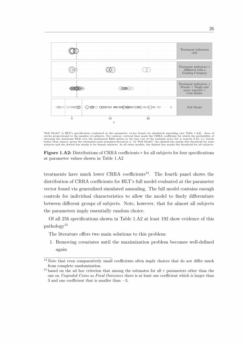
26

Treatment indicatorsonly

Treatment indicators +Affiliated with aGrading Company

Treatment indicators +Female + Single andnever married +Coin Dealer

Full Model

0 10 20r

“Full Model” is HLT’s specification evaluated at the parameter vector found via simulated annealing (see Table 1.A2). Area ofcircles proportional to the number of subjects. For context, vertical lines mark the CRRA coefficient for which the probability ofchoosing the dominant $350 over the dominated $200 option in the last row of the multiple price list is exactly 0.55, i.e. barelybetter than chance, given the estimated noise standard deviation σ. In “Full Model”, the dashed line marks this threshold for malesubjects and the dotted line marks it for female subjects. In all other models, the dashed line marks the threshold for all subjects.

Figure 1.A2: Distributions of CRRA coefficients r for all subjects for four specificationsat parameter values shown in Table 1.A2

treatments have much lower CRRA coefficients14. The fourth panel shows thedistribution of CRRA coefficients for HLT’s full model evaluated at the parametervector found via generalized simulated annealing. The full model contains enoughcontrols for individual characteristics to allow the model to finely differentiatebetween different groups of subjects. Note, however, that for almost all subjectsthe parameters imply essentially random choice.

Of all 256 specifications shown in Table 1.A2 at least 192 show evidence of thispathology15

The literature offers two main solutions to this problem:

1. Removing covariates until the maximization problem becomes well-definedagain

14 Note that even comparatively small coefficients often imply choices that do not differ muchfrom complete randomization.

15 based on the ad hoc criterion that among the estimates for all r parameters other than theone on Ungraded Coins as Final Outcomes there is at least one coefficient which is larger than3 and one coefficient that is smaller than −3.

27

2. Penalized likelihood estimation (Firth, 1993), a procedure in which a termthat penalizes extreme parameter values is added to the log-likelihood. Thisensures that the entire maximization problem is guaranteed to have a globalmaximum even if the likelihood function does not.

Neither of these solutions is ideal. In as far as covariates help predict the de-pendent variable their removal may restore identification but introduce bias at thesame time. Penalized likelihood estimation, on the other hand, will ensure the ex-istence of a maximum but do so by essentially imposing specific values on groupsof parameters (how far the parameters are allowed to move away from each otherwill depend on how high the penalty for large parameter values is), some of whichare the treatment indicators which are of main inferential interest.

Likelihood maximization — Methodology

The estimates displayed in Table 1.A2 are the results of extensive efforts to maxi-mize the log-likelihood functions associated with all 256 specifications. Numericalmaximization was performed using a number of different approaches that differ inthe maximization algorithm used and in the way the algorithms are initialized.

First, I use a variety of maximization algorithms that break down into twoclasses:

• hill-climbing methods: These include simplex methods like Nelder-Mead,gradient ascent methods like BFGS, CG (conjugate gradient), nlminb (a gra-dient ascent method using PORT routines), spg (spectral projected gradient)and ucminf, and derivative-free methods using trust regions like newuoa,bobyqa, and using other techniques like the Hooke-Jeeves algorithm forderivative-free optimization. All methods are provided by R’s optimx pack-age (Nash & Varadhan, 2011). These algorithms are generally fast to con-verge to an optimum but may get stuck in local optima if the likelihoodfunction is not globally concave, in which case the value at which the pa-rameter vector is initialized may matter.16

• generalized simulated annealing as implemented by R’s GenSA package(Yang Xiang, Gubian, Suomela, & Hoeng, 2013). Simulated annealing (Kirk-

16 Implementation details: All algorithms were run for a maximum of 2500 iterations with defaultcriteria and threshold for convergence.

28

patrick, Gelatt, P., & Vecchi, 1983) is a method that takes random jumpsthrough the parameter space in search of higher values of the objective func-tion and in which the size of these jumps is reduced over time. This methodis generally more robust to getting stuck in local optima but is very slow.17

Second, to further reduce the likelihood of getting stuck in local optima or to missoptima, each of the above maximization algorithms were initialized in two differentways:

• independent: All parameters in the r equation were set to 0 and all pa-rameters in the noise equation were set to 2.72 (e).18

• iterative: For each specification, the results from all nested specificationswere gathered and from this set the result with the highest log-likelihood wasselected. The maximization algorithm was then initialized at this parametervector while setting the parameters not contained in the nested model tozero.

For each of the 256 specifications, Table 1.A2 shows the parameter vector whichachieves the highest log-likelihood among all maximization algorithm and amongall initialization procedures, no matter whether the algorithm in question success-fully converged.

17 Implementation details: the algorithm searched for optima in a hypercube, with all r-parameters in the interval [−15, 15] and all σ-parameters in the interval [exp(−20), exp(20)].The algorithm was run for a maximum of 100, 000 iterations and would stop if no improvementhad occurred for 5, 000 steps.

18 where, again, noise parameters are on the same scale as reported in HLT for comparability

29r-variables included (inaddition to treatmentindicators)

σ-variablesincluded

r σ

constant coins ungraded skewLO skewHI female college single ms dealer dcoins grcomp constant female LL N

Full Model (original estimates) female 0.95 -0.16 3.75 0.76 0.14 -1.26 0.04 0.84 0.03 -0.98 0.39 -0.12 0.41 12.54 -1486.29 2259

TI only 0.10 0.19 0.85 -0.15 -0.10 2.05 -1534.74 2259

female -0.04 0.09 2.02 -0.20 -0.19 -0.20 11.19 -1514.48 2239

college 0.04 0.19 1.06 -0.17 -0.12 0.04 2.68 -1534.46 2259

single 0.10 0.19 0.79 -0.15 -0.11 -0.03 2.06 -1534.68 2259

ms 0.09 0.19 0.86 -0.15 -0.10 0.01 2.05 -1534.74 2259

dealer 0.20 0.21 0.99 0.07 0.07 -0.38 1.38 -1511.45 2259

dealer.coins 0.10 0.55 0.86 -0.09 -0.02 -0.56 1.49 -1527.30 2259

grcomp 9.41 10.61 -0.88 -9.41 -9.37 -9.48 1.54 -1530.47 2259

female, college 14.96 -3.48 4.28 -5.69 -7.13 -4.59 -3.06 0.01 -1506.29 2239

female, single 14.73-13.38

1.06 6.00 14.41 13.18 -7.05 0.00 -1501.25 2239

female, ms 1.47 0.48 2.12 -0.17 -0.99 -1.07 -0.94 38.60 -1503.15 2239

female, dealer 0.12 0.19 1.21 0.04 -0.00 -0.13 -0.32 2.45 -1496.08 2239

female, dealer.coins -0.06 0.30 1.20 -0.14 -0.07 -0.16 -0.37 6.80 -1508.36 2239

female, grcomp 15.00 -2.87 4.42 -2.30 -5.38 -9.56 -5.59 0.91 -1502.84 2239

college, single 14.83 -9.59 -0.13 3.63 6.63 11.43 -8.61 0.00 -1519.59 2259

college, ms 15.00 -3.41 -5.16 -8.28 7.38 6.22 1.93 0.00 -1533.77 2259

college, dealer 0.21 0.19 1.04 0.08 0.08 0.03 -0.40 1.38 -1511.37 2259

30

r-variables included (inaddition to treatmentindicators)

σ-variablesincluded

r σ

constant coins ungraded skewLO skewHI female college single ms dealer dcoins grcomp constant female LL N

Full Model (original estimates) female 0.95 -0.16 3.75 0.76 0.14 -1.26 0.04 0.84 0.03 -0.98 0.39 -0.12 0.41 12.54 -1486.29 2259

college, dealer.coins -0.08 0.76 1.08 -0.12 -0.04 0.13 -0.82 3.66 -1524.12 2259

college, grcomp 9.16 -3.02 5.53 0.03 5.65 -3.60 -5.60 0.00 -1502.54 2259

single, ms 15.00 3.68 -9.65 2.16 5.21 -8.01 -3.19 0.00 -1513.55 2259

single, dealer 0.21 0.22 0.96 0.09 0.08 0.02 -0.39 1.35 -1511.41 2259

single, dealer.coins 14.82 -3.00 2.38 -2.88 5.89 -8.61 -9.10 0.00 -1516.32 2259

single, grcomp 15.00 -7.13 4.27 -3.77 2.27 -3.83 -7.26 0.00 -1522.61 2259

ms, dealer 0.09 0.22 1.05 0.07 0.04 0.14 -0.41 1.46 -1510.84 2259

ms, dealer.coins 0.11 0.54 0.85 -0.09 -0.01 -0.02 -0.56 1.48 -1527.27 2259

ms, grcomp 9.02 10.28 -0.91 -9.05 -9.05 0.08 -9.17 1.47 -1529.49 2259

dealer, dealer.coins 0.15 0.61 0.95 0.06 0.06 -0.33 -0.41 1.54 -1510.60 2259

dealer, grcomp 0.20 0.21 1.00 0.08 0.07 -0.38 0.01 1.39 -1511.45 2259

dealer.coins, grcomp 0.10 0.54 0.89 -0.10 -0.03 -0.56 0.02 1.48 -1527.28 2259

female, college, single123.69

-101.18

22.45 50.89220.58 753.41 -13.37 -73.12

0.00 -1490.90 2239

female, college, ms 15.00 2.41 3.81 1.88 -5.16 -7.14 -2.56 -5.34 0.00 -1478.10 2239

female, college, dealer 0.10 0.18 1.26 0.03 0.00 -0.13 0.02 -0.32 2.59 -1496.02 2239

female, college, dealer.coins 15.00 -2.71 5.25 -5.51 0.25 -4.79 -2.85 -7.98 0.00 -1499.91 2239

female, college, grcomp 13.89 -4.44 8.77 0.03 8.87 -0.00 -5.09 -8.84 0.00 -1486.83 2239

31r-variables included (inaddition to treatmentindicators)

σ-variablesincluded

r σ

constant coins ungraded skewLO skewHI female college single ms dealer dcoins grcomp constant female LL N

Full Model (original estimates) female 0.95 -0.16 3.75 0.76 0.14 -1.26 0.04 0.84 0.03 -0.98 0.39 -0.12 0.41 12.54 -1486.29 2259

female, single, ms 15.00 -3.71 -3.27 3.05 6.02 7.29 -7.82 -3.25 0.00 -1492.03 2239

female, single, dealer 1.05 0.24 12.77 0.90 0.17 -0.75 0.83 -1.23 0.98 -1490.39 2239

female, single, dealer.coins 14.98 -5.07 4.19 -5.04 0.09 -2.51 -4.55 -7.72 0.00 -1493.60 2239

female, single, grcomp 13.87-11.98

1.67 5.66 14.73 14.35 -7.29 -1.31 0.00 -1491.28 2239

female, ms, dealer 0.06 0.20 1.22 0.05 0.00 -0.11 0.07 -0.35 2.44 -1495.80 2239

female, ms, dealer.coins 2.79 1.05 2.01 -0.17 -1.61 -1.69 -1.56 -0.94 24.32 -1501.80 2239

female, ms, grcomp 14.98 4.64 2.70 -3.25 -9.12 -6.12 -5.99 -3.33 6.08 -1491.62 2239

female, dealer, dealer.coins 0.08 0.47 1.08 0.04 0.01 -0.11 -0.30 -0.29 2.60 -1495.46 2239

female, dealer, grcomp 0.13 0.18 1.35 0.07 0.00 -0.14 -0.35 0.05 2.45 -1495.72 2239

female, dealer.coins, grcomp 14.99 -2.92 4.48 -2.34 -5.48 -9.45 0.37 -5.69 0.91 -1502.84 2239

college, single, ms 15.28 3.55-10.01

2.38 5.35 -0.11 -7.91 -3.18 0.00 -1511.74 2259

college, single, dealer 15.00 -6.57 3.71 -4.20 0.27 -1.99 -3.90 -4.69 0.00 -1510.86 2259

college, single, dealer.coins 14.90 -4.98 -0.21 -4.73 3.24 3.41 -4.87 -5.15 0.00 -1510.67 2259

college, single, grcomp 9.13 -3.03 5.57 0.10 5.67 -3.62 2.07 -5.56 0.00 -1499.78 2259

college, ms, dealer 15.00 -3.92 -4.50 -9.27 -2.03 6.74 2.82 -4.12 0.00 -1507.90 2259

college, ms, dealer.coins 15.00 6.82-14.89

-9.05 -2.04 6.47 2.25 -3.67 0.00 -1507.65 2259

college, ms, grcomp 9.63 -3.21 5.72 0.05 5.84 -3.75 -0.16 -5.76 0.00 -1502.17 2259

32

r-variables included (inaddition to treatmentindicators)

σ-variablesincluded

r σ

constant coins ungraded skewLO skewHI female college single ms dealer dcoins grcomp constant female LL N

Full Model (original estimates) female 0.95 -0.16 3.75 0.76 0.14 -1.26 0.04 0.84 0.03 -0.98 0.39 -0.12 0.41 12.54 -1486.29 2259

college, dealer, dealer.coins 0.13 0.63 0.97 0.06 0.07 0.03 -0.33 -0.46 1.62 -1510.41 2259

college, dealer, grcomp 11.46 -3.62 7.17 0.03 7.28 -4.26 0.00 -7.23 0.00 -1500.75 2259

college, dealer.coins, grcomp 12.95 0.10 11.66 -4.97 7.35 -6.02 -5.55 -6.97 0.00 -1487.78 2259

single, ms, dealer 15.00 3.23 -9.63 2.27 5.50 -7.76 -3.11 -0.41 0.00 -1509.29 2259

single, ms, dealer.coins 14.93 2.99 -9.77 2.08 5.69 -7.00 -3.22 -0.67 0.00 -1508.98 2259

single, ms, grcomp 13.91 -2.88 -0.32 -3.46 -1.13 -4.85 -2.40 -3.65 0.00 -1502.44 2259

single, dealer, dealer.coins 0.15 0.62 0.91 0.07 0.07 0.02 -0.34 -0.42 1.52 -1510.56 2259

single, dealer, grcomp 0.21 0.22 0.94 0.09 0.08 0.03 -0.39 -0.01 1.34 -1511.41 2259

single, dealer.coins, grcomp 14.49 -3.11 4.58 -3.78 2.27 -7.28 -8.45 -2.33 0.00 -1507.77 2259

ms, dealer, dealer.coins 0.05 0.70 0.97 0.06 0.04 0.13 -0.37 -0.49 1.60 -1509.84 2259

ms, dealer, grcomp 0.09 0.22 1.07 0.07 0.04 0.14 -0.41 0.01 1.46 -1510.83 2259

ms, dealer.coins, grcomp 0.11 0.54 0.87 -0.09 -0.02 -0.01 -0.56 0.01 1.48 -1527.26 2259

dealer, dealer.coins, grcomp 0.15 0.61 0.96 0.06 0.06 -0.33 -0.41 0.01 1.55 -1510.59 2259

female, college, single, ms 19.10 2.92 4.99 2.28 -6.65 -9.01 -3.26 1.70 -7.06 0.00 -1477.37 2239

female, college, single, dealer 15.00 1.20-10.27 -10.01

-6.15 13.36 8.31 4.22 -1.03 0.00 -1485.39 2239

female, college, single,dealer.coins

14.98 2.82-11.35 -10.95

-6.68 13.60 9.12 4.62 -1.26 0.00 -1481.91 2239

33r-variables included (inaddition to treatmentindicators)

σ-variablesincluded

r σ

constant coins ungraded skewLO skewHI female college single ms dealer dcoins grcomp constant female LL N

Full Model (original estimates) female 0.95 -0.16 3.75 0.76 0.14 -1.26 0.04 0.84 0.03 -0.98 0.39 -0.12 0.41 12.54 -1486.29 2259

female, college, single, grcomp 9.56-14.23

8.90 11.24 7.33 12.48 7.08 -6.26 5.13 0.00 -1465.28 2239

female, college, ms, dealer 18.50 2.60 5.29 0.76 -6.84 -8.94 -2.59 -7.02 1.46 0.00 -1468.45 2239

female, college, ms,dealer.coins

15.00 3.50 1.97 2.10 -4.40 -6.60 -3.86 -4.58 -3.61 0.00 -1474.32 2239

female, college, ms, grcomp 33.70 4.55 6.52 -0.72-14.48 -13.82

-5.17-10.20

-4.58 0.00 -1476.05 2239

female, college, dealer,dealer.coins

0.02 0.53 1.12 0.01 0.02 -0.11 0.04 -0.28 -0.39 3.26 -1495.09 2239

female, college, dealer, grcomp 13.89 -4.44 8.77 0.03 8.88 -0.00 -5.09 -0.00 -8.84 0.00 -1486.82 2239

female, college, dealer.coins,grcomp

6.35 6.30 4.74 -1.45 3.95 -0.35 -2.65 -8.50 -3.58 0.00 -1474.82 2239

female, single, ms, dealer 14.54-11.58

-0.28 6.47 12.12 13.09 -7.77 -1.37 13.55 0.00 -1488.27 2239

female, single, ms, dealer.coins 15.00 -2.06 -8.06 2.34 -2.63 7.55 -4.75 -2.48 7.03 0.00 -1484.56 2239

female, single, ms, grcomp 15.00 -4.81 -0.33 2.05 4.44 14.20 -9.31 -2.61 -4.37 0.00 -1483.94 2239

female, single, dealer,dealer.coins

8.80 -8.00 0.20 3.33 4.93 4.25 -4.16 -8.74 8.24 0.28 -1481.24 2239

female, single, dealer, grcomp 4.16 0.26 5.52 4.03 0.23 -3.90 4.11 -4.26 -0.15 0.70 -1488.98 2239

female, single, dealer.coins, gr-comp

12.98 -9.64 3.27 5.57 14.73 14.35 -8.64 0.28 -3.04 0.00 -1487.87 2239

female, ms, dealer, dealer.coins 0.01 0.58 1.06 0.04 0.01 -0.09 0.09 -0.33 -0.40 2.66 -1495.07 2239

female, ms, dealer, grcomp 14.97 4.61 2.72 -3.27 -9.12 -6.12 -5.99 0.06 -3.38 6.20 -1491.35 2239

34

r-variables included (inaddition to treatmentindicators)

σ-variablesincluded

r σ

constant coins ungraded skewLO skewHI female college single ms dealer dcoins grcomp constant female LL N

Full Model (original estimates) female 0.95 -0.16 3.75 0.76 0.14 -1.26 0.04 0.84 0.03 -0.98 0.39 -0.12 0.41 12.54 -1486.29 2259

female, ms, dealer.coins, gr-comp

14.96 4.47 2.80 -3.36 -9.17 -6.05 -5.93 0.38 -3.45 6.07 -1491.62 2239

female, dealer, dealer.coins, gr-comp

0.08 0.45 1.17 0.06 0.01 -0.12 -0.32 -0.27 0.04 2.63 -1495.21 2239

college, single, ms, dealer 14.74 -3.49 -4.48 -8.63 -1.24 6.97 -0.70 2.54 -3.73 0.00 -1505.17 2259

college, single, ms, dealer.coins 16.66 6.30-14.17 -10.64

-1.85 6.77 -0.20 2.05 -4.91 0.00 -1506.62 2259

college, single, ms, grcomp 9.23 -3.01 5.57 0.16 5.66 -3.52 2.07 -0.25 -5.50 0.00 -1498.60 2259

college, single, dealer,dealer.coins

0.13 0.65 0.92 0.07 0.08 0.04 0.03 -0.34 -0.47 1.59 -1510.35 2259

college, single, dealer, grcomp 9.71 -3.05 6.21 0.11 6.31 -3.55 2.08 0.00 -6.20 0.00 -1498.01 2259

college, single, dealer.coins, gr-comp

5.33 0.14 4.07 -1.20 3.51 -2.24 9.30 -1.77 -3.13 0.00 -1486.53 2259

college, ms, dealer, dealer.coins 15.81 5.17-13.43

-9.59 -2.08 7.06 2.09 2.56 -6.09 0.00 -1507.28 2259

college, ms, dealer, grcomp 13.84-13.04

4.32 -6.98 3.14 3.04 8.14-11.04

2.59 0.01 -1493.92 2259

college, ms, dealer.coins, gr-comp

12.74 0.06 11.57 -4.89 7.33 -5.96 0.13 -5.48 -6.96 0.00 -1487.43 2259

college, dealer, dealer.coins, gr-comp

6.60 0.16 5.42 -1.78 4.29 -2.92 0.35 -2.71 -3.91 0.00 -1484.79 2259

single, ms, dealer, dealer.coins 13.85 -2.99 -0.33 -4.07 0.10 -3.78 -2.68 7.68 -9.42 0.00 -1496.71 2259

single, ms, dealer, grcomp 14.32 -2.91 -0.33 -3.71 -0.92 -4.91 -2.47 -0.55 -3.22 0.00 -1497.42 2259

single, ms, dealer.coins, gr-comp

13.83 -2.95 -0.33 -3.36 -0.72 -4.82 -2.38 -0.48 -3.19 0.00 -1498.02 2259

35r-variables included (inaddition to treatmentindicators)

σ-variablesincluded

r σ

constant coins ungraded skewLO skewHI female college single ms dealer dcoins grcomp constant female LL N

Full Model (original estimates) female 0.95 -0.16 3.75 0.76 0.14 -1.26 0.04 0.84 0.03 -0.98 0.39 -0.12 0.41 12.54 -1486.29 2259

single, dealer, dealer.coins, gr-comp

15.90 -4.14 4.14 -3.65 3.18 -7.78 0.34 -8.24 -3.24 0.00 -1506.20 2259

ms, dealer, dealer.coins, gr-comp

0.05 0.70 0.99 0.07 0.04 0.14 -0.37 -0.50 0.01 1.62 -1509.82 2259

female, college, single, ms,dealer

112.4436.39 15.16 0.87

-50.26 -54.73-7.16 50.69

-50.746.54 0.00 -1467.32 2239

female, college, single, ms,dealer.coins

23.07 6.22 1.20 3.87 -6.35-10.26

-6.16 -1.53 -6.75 -6.23 0.00 -1470.11 2239

female, college, single, ms, gr-comp

9.70-14.10

8.83 11.12 7.55 13.95 7.20 -6.06 -0.39 5.35 0.00 -1459.81 2239

female, college, single, dealer,dealer.coins

6.56 -5.85 0.17 2.80 4.38 3.67 0.07 -3.56 -6.54 6.09 0.29 -1480.51 2239

female, college, single, dealer,grcomp

10.29-14.69

8.50 10.79 7.65 16.15 7.44 -6.13 0.06 4.82 0.00 -1464.67 2239

female, college, single,dealer.coins, grcomp

10.29-14.69

8.50 10.79 7.65 16.15 7.44 -6.13 0.06 4.82 0.00 -1464.67 2239

female, college, ms, dealer,dealer.coins

21.73 6.28 1.20 0.82 -6.41 -9.22 -5.80 -6.81 2.31 -8.65 0.00 -1464.57 2239

female, college, ms, dealer, gr-comp

22.01 1.55 6.53 -1.23 -9.03 -9.52 -3.30 -7.21 1.96 -2.03 0.00 -1467.39 2239

female, college, ms,dealer.coins, grcomp

6.89 -6.08 5.23 -7.89 12.89 13.06 3.29 9.10-11.93

2.52 0.00 -1470.58 2239

female, college, dealer,dealer.coins, grcomp

5.90 6.38 4.45 -1.31 3.80 -0.21 -2.49 0.14 -8.43 -3.42 0.00 -1474.40 2239

female, single, ms, dealer,dealer.coins

9.03 -7.97 0.04 3.45 4.94 4.19 -4.10 -0.46 -8.49 8.30 0.25 -1474.32 2239

female, single, ms, dealer, gr-comp

15.00 -5.92 -0.27 2.49 5.64 13.03 -8.49 -2.82 -0.59 -2.33 0.00 -1481.85 2239

36

r-variables included (inaddition to treatmentindicators)

σ-variablesincluded

r σ

constant coins ungraded skewLO skewHI female college single ms dealer dcoins grcomp constant female LL N

Full Model (original estimates) female 0.95 -0.16 3.75 0.76 0.14 -1.26 0.04 0.84 0.03 -0.98 0.39 -0.12 0.41 12.54 -1486.29 2259

female, single, ms, dealer.coins,grcomp

15.00 -4.81 -0.32 2.02 4.46 14.20 -9.29 -2.60 -0.07 -4.37 0.00 -1483.60 2239

female, single, dealer,dealer.coins, grcomp

9.06 -8.23 0.26 3.21 4.58 4.30 -4.01 -8.80 8.45 -0.27 0.14 -1476.01 2239

female, ms, dealer,dealer.coins, grcomp

14.95 4.48 2.80 -3.35 -9.15 -6.07 -5.94 0.06 0.32 -3.46 6.20 -1491.35 2239

college, single, ms, dealer,dealer.coins

56.86 -8.17 -0.32-18.58

5.13 -0.00-22.75

-7.06 0.07-17.03

0.00 -1492.74 2259

college, single, ms, dealer, gr-comp

14.35-13.22

4.18 -7.16 3.42 3.40 -0.82 7.19-10.99

3.02 0.02 -1488.15 2259

college, single, ms,dealer.coins, grcomp

11.89 -7.42 -0.29 -6.03 -0.86 7.40 -3.22 5.08 -3.13 -5.92 0.00 -1485.74 2259

college, single, dealer,dealer.coins, grcomp

5.50 0.22 4.31 -1.27 3.69 -2.42 3.05 0.35 -2.20 -3.31 0.00 -1482.72 2259

college, ms, dealer,dealer.coins, grcomp

5.52 0.13 4.27 -1.20 3.73 -2.44 0.05 0.35 -2.12 -3.35 0.00 -1484.69 2259

single, ms, dealer, dealer.coins,grcomp

13.87 -3.00 -0.30 -4.06 0.10 -3.81 -2.71 7.68 -9.42 -0.00 0.00 -1496.70 2259

female, college, single, ms,dealer, dealer.coins

21.56 5.87 1.19 0.66 -6.05 -9.29 -5.92 -1.46 -6.39 2.95 -8.88 0.00 -1460.23 2239

female, college, single, ms,dealer, grcomp

9.83-14.23

8.85 11.14 7.60 13.95 7.30 -5.99 -0.48 0.22 5.27 0.00 -1454.46 2239

female, college, single, ms,dealer.coins, grcomp

9.89-14.15

8.84 11.13 7.53 13.95 7.25 -6.01 -0.60 0.24 5.23 0.00 -1454.28 2239

female, college, single, dealer,dealer.coins, grcomp

10.62-14.89

8.64 10.95 7.56 16.28 7.36 -6.39 0.08 -0.02 4.82 0.00 -1464.56 2239

female, college, ms, dealer,dealer.coins, grcomp

22.44 7.27 1.25 0.87 -7.27 -9.60 -5.40 -7.68 1.68 -9.17 0.19 0.00 -1464.22 2239

37r-variables included (inaddition to treatmentindicators)

σ-variablesincluded

r σ

constant coins ungraded skewLO skewHI female college single ms dealer dcoins grcomp constant female LL N

Full Model (original estimates) female 0.95 -0.16 3.75 0.76 0.14 -1.26 0.04 0.84 0.03 -0.98 0.39 -0.12 0.41 12.54 -1486.29 2259

female, single, ms, dealer,dealer.coins, grcomp

9.08 -7.99 0.08 3.43 4.77 4.38 -4.09 -0.43 -8.40 8.31 -0.26 0.15 -1469.88 2239

college, single, ms, dealer,dealer.coins, grcomp

5.55 0.25 4.34 -1.30 3.68 -2.42 3.05 -0.07 0.35 -2.23 -3.30 0.00 -1482.58 2259

female, college, single, ms,dealer, dealer.coins, grcomp

9.98-14.20

8.82 11.22 7.66 13.91 7.32 -5.97 -0.70 0.14 0.21 5.04 0.00 -1453.13 2239

TI only female -0.02 0.20 0.90 -0.18 -0.10 3.91 0.00 -1519.34 2239

female female 0.60 0.07 0.74 -0.13 -0.16 -1.96 0.21 >100 -1506.54 2239

college female -0.06 0.20 1.05 -0.19 -0.11 0.03 4.78 0.00 -1519.11 2239

single female 11.64-10.35

0.99 3.31 12.63 -4.31 0.00 >100 -1501.33 2239

ms female -0.06 0.19 0.99 -0.21 -0.14 0.06 4.66 0.00 -1518.77 2239

dealer female 0.17 0.22 1.01 0.07 0.07 -0.38 1.63 0.00 -1498.06 2239

dealer.coins female -0.01 0.56 0.93 -0.12 -0.02 -0.57 2.82 0.00 -1512.32 2239

grcomp female 6.99 8.44 -0.87 -7.15 -7.08 -7.19 3.17 0.00 -1515.45 2239

female, college female 0.45 0.11 0.81 -0.15 -0.14 -2.54 0.05 0.34 >100 -1506.06 2239

female, single female 14.67-13.32

1.06 6.51 14.38 9.09 -7.57 0.00 >100 -1501.25 2239

female, ms female 1.44 0.16 1.36 -0.14 -0.43 -2.01 -0.38 0.06 >100 -1500.20 2239

female, dealer female 0.43 0.14 0.85 0.01 -0.03 -1.11 -0.26 0.39 95.54 -1491.27 2239

female, dealer.coins female 14.79 10.99 -0.48 -9.47 -9.36 -6.73-11.41

0.00 >100 -1494.75 2239

38

r-variables included (inaddition to treatmentindicators)

σ-variablesincluded

r σ

constant coins ungraded skewLO skewHI female college single ms dealer dcoins grcomp constant female LL N

Full Model (original estimates) female 0.95 -0.16 3.75 0.76 0.14 -1.26 0.04 0.84 0.03 -0.98 0.39 -0.12 0.41 12.54 -1486.29 2259

female, grcomp female 15.00 -2.12 3.68 -1.57 -3.90-11.04

-4.12 0.00 0.92 -1501.13 2239

college, single female 30.41-22.25

8.05 12.42 22.23 -3.50-20.25

0.00 >100 -1490.91 2239

college, ms female 1.51 8.27 -7.94 -4.87 -4.92 3.48 3.64 0.29 >100 -1503.48 2239

college, dealer female 0.21 0.18 1.07 0.09 0.09 0.04 -0.42 1.54 0.00 -1497.96 2239

college, dealer.coins female 0.01 2.68 -3.29 -0.23 -0.64 1.01 2.50 40.83 >100 -1508.64 2239

college, grcomp female 7.20 -2.15 4.65 0.25 4.69 -2.75 -4.49 0.00 0.04 -1479.88 2239

single, ms female 12.25 -7.41 -0.27 3.00 4.96 -5.47 -2.12 0.00 >100 -1485.93 2239

single, dealer female 14.48 -3.86 2.65 -3.21 4.05 -7.09 -7.62 0.00 2.01 -1495.98 2239

single, dealer.coins female 11.81-10.80

0.44 3.67 4.72 -4.44 -0.27 0.02 >100 -1499.47 2239

single, grcomp female 11.62 -9.73 1.67 4.32 12.63 -5.95 -1.31 0.00 >100 -1491.28 2239

ms, dealer female 0.01 0.23 1.09 0.05 0.03 0.16 -0.39 2.07 0.00 -1497.24 2239

ms, dealer.coins female -0.06 0.58 0.95 -0.13 -0.04 0.04 -0.59 3.15 0.00 -1512.10 2239

ms, grcomp female 12.45 14.10 -0.89-12.74 -12.68

0.12-12.82

4.41 0.00 -1513.09 2239

dealer, dealer.coins female 0.10 0.64 0.97 0.05 0.06 -0.32 -0.44 1.94 0.00 -1497.12 2239

dealer, grcomp female 0.17 0.22 1.03 0.07 0.07 -0.38 0.01 1.64 0.00 -1498.05 2239

dealer.coins, grcomp female -0.01 0.55 0.95 -0.12 -0.03 -0.57 0.01 2.81 0.00 -1512.31 2239

female, college, single female 14.99 8.46-11.41 -13.90

-1.10 -4.96 3.44 1.91 0.01 >100 -1485.36 2239

39r-variables included (inaddition to treatmentindicators)

σ-variablesincluded

r σ

constant coins ungraded skewLO skewHI female college single ms dealer dcoins grcomp constant female LL N

Full Model (original estimates) female 0.95 -0.16 3.75 0.76 0.14 -1.26 0.04 0.84 0.03 -0.98 0.39 -0.12 0.41 12.54 -1486.29 2259

female, college, ms female 29.90 4.87 7.05 2.19-10.85 -13.13

-5.79-11.02

0.00 0.00 -1477.19 2239

female, college, dealer female 0.37 0.12 0.94 -0.02 -0.02 -1.34 0.06 -0.25 0.46 >100 -1490.42 2239

female, college, dealer.coins female 21.51 9.72 -1.27 -6.10 -3.12-27.56

0.86-12.78

0.00 >100 -1483.17 2239

female, college, grcomp female 11.32 -3.58 7.34 0.27 7.37 -0.33 -4.04 -7.15 0.00 0.02 -1478.25 2239

female, single, ms female 14.94 -8.63 -0.33 2.72 5.29 -3.32 -5.85 -2.85 0.00 >100 -1483.16 2239

female, single, dealer female 13.28 -4.99 2.86 -4.02 0.75 -4.09 -4.01 -5.30 0.00 1.27 -1482.38 2239

female, single, dealer.coins female 67.76-23.44

18.45-24.92

0.17-11.60 -19.07 -33.13

0.00 0.00 -1489.97 2239

female, single, grcomp female 13.87-11.98

1.67 5.66 15.73 15.35 -7.29 -1.31 0.00 0.00 -1491.28 2239

female, ms, dealer female 0.39 0.15 0.85 0.01 -0.02 -1.09 0.02 -0.27 0.41 99.71 -1491.22 2239

female, ms, dealer.coins female 0.89 0.20 0.56 -0.08 -0.09 -2.21 -0.10 -0.34 0.07 >100 -1494.32 2239

female, ms, grcomp female 14.76 3.89 3.32 -2.91 -8.64 -6.41 -5.84 -3.00 0.53 6.50 -1491.40 2239

female, dealer, dealer.coins female 0.38 0.30 0.77 -0.01 -0.01 -1.20 -0.22 -0.19 0.42 >100 -1490.40 2239

female, dealer, grcomp female 0.43 0.14 0.94 0.03 -0.03 -1.17 -0.28 0.04 0.39 >100 -1491.00 2239

female, dealer.coins, grcomp female 5.46 0.53 2.10 -1.40 1.52 -4.72 -3.88 -1.51 0.00 38.88 -1483.18 2239

college, single, ms female 12.50 -7.16 -0.13 2.64 4.99 -0.21 -5.21 -2.51 0.00 >100 -1479.76 2239

college, single, dealer female 14.82 5.85-14.99

-9.84 -5.97 8.30 4.28 -1.13 0.00 >100 -1485.52 2239

college, single, dealer.coins female 14.60 2.42-10.94 -11.09

-6.95 9.31 5.14 -1.51 0.00 >100 -1482.77 2239

40

r-variables included (inaddition to treatmentindicators)

σ-variablesincluded

r σ

constant coins ungraded skewLO skewHI female college single ms dealer dcoins grcomp constant female LL N

Full Model (original estimates) female 0.95 -0.16 3.75 0.76 0.14 -1.26 0.04 0.84 0.03 -0.98 0.39 -0.12 0.41 12.54 -1486.29 2259

college, single, grcomp female 9.44-12.17

4.41 6.73 4.13 3.93 -3.71 3.24 0.00 >100 -1476.36 2239

college, ms, dealer female 12.07 0.46 -7.19 -7.24 -1.69 5.81 2.03 -2.41 0.00 >100 -1487.74 2239

college, ms, dealer.coins female 13.17 8.97-13.78 -14.84

-3.28 11.16 6.61 -7.76 0.00 >100 -1479.51 2239

college, ms, grcomp female 9.40 -2.83 6.01 0.47 5.89 -3.47 -0.38 -5.58 0.00 0.04 -1474.55 2239

college, dealer, dealer.coins female 0.09 0.66 1.00 0.06 0.06 0.03 -0.32 -0.49 2.01 0.00 -1496.94 2239

college, dealer, grcomp female 16.25 -5.22 10.63 0.28 10.64 -5.86 0.00-10.43

0.00 0.00 -1478.13 2239

college, dealer.coins, grcomp female 6.65 11.47 5.29 -1.72 4.24 -2.83-13.79

-3.86 0.00 0.00 -1477.37 2239

single, ms, dealer female 15.48 -7.88 -0.29 2.02 5.29 -6.50 -2.84 -0.69 0.00 >100 -1482.13 2239

single, ms, dealer.coins female 15.48 -7.88 -0.29 2.02 5.29 -6.50 -2.84 -0.69 0.00 >100 -1482.13 2239

single, ms, grcomp female 12.98 -7.61 -0.33 2.88 5.02 -5.63 -2.30 -0.07 0.00 >100 -1484.77 2239

single, dealer, dealer.coins female 10.40 -0.58 -9.70 2.04 0.15 -2.15-10.48

13.61 0.59 >100 -1490.50 2239

single, dealer, grcomp female 14.92 -6.09 3.54 -1.39 3.18 -7.18 -4.97 -3.25 0.00 8.67 -1482.03 2239

single, dealer.coins, grcomp female 11.71 -9.65 1.94 4.24 12.63 -6.02 0.20 -1.66 0.00 >100 -1489.34 2239

ms, dealer, dealer.coins female -0.04 0.77 1.01 0.04 0.03 0.15 -0.35 -0.56 2.39 0.00 -1496.03 2239

ms, dealer, grcomp female 0.01 0.23 1.10 0.05 0.03 0.16 -0.39 0.00 2.07 0.00 -1497.23 2239

ms, dealer.coins, grcomp female 14.20 -9.28 4.93 2.03 5.37 -0.96 0.96 -4.47 0.00 >100 -1508.16 2239

dealer, dealer.coins, grcomp female 0.10 0.65 0.99 0.06 0.06 -0.32 -0.45 0.01 1.95 0.00 -1497.11 2239

41r-variables included (inaddition to treatmentindicators)

σ-variablesincluded

r σ

constant coins ungraded skewLO skewHI female college single ms dealer dcoins grcomp constant female LL N

Full Model (original estimates) female 0.95 -0.16 3.75 0.76 0.14 -1.26 0.04 0.84 0.03 -0.98 0.39 -0.12 0.41 12.54 -1486.29 2259

female, college, single, ms female 29.90 4.87 7.05 2.19-10.85 -13.13

-5.79 0.00-11.02

0.00 0.00 -1477.19 2239

female, college, single, dealer female 22.36 -7.70 6.49 -7.15 0.27 -7.40 -0.05 -7.18 -7.99 0.00 2.40 -1480.24 2239

female, college, single,dealer.coins

female 15.00 1.91 -7.67-11.87

-4.55 -6.27 9.28 2.76 -4.98 0.00 >100 -1463.01 2239

female, college, single, grcomp female 12.40-17.37

9.11 11.41 8.14 10.92 7.89 -6.16 5.45 0.00 0.00 -1464.90 2239

female, college, ms, dealer female 34.78 8.20 7.02 0.78-14.12 -16.64

-3.75-14.44

2.00 0.00 0.00 -1467.39 2239

female, college, ms,dealer.coins

female 15.76 4.32 1.25 2.12 -4.49 -6.71 -4.43 -4.68 -4.43 0.00 0.00 -1474.28 2239

female, college, ms, grcomp female 9.39 -2.83 6.01 0.47 5.89 -0.09 -3.46 -0.38 -5.59 0.00 0.03 -1473.86 2239

female, college, dealer,dealer.coins

female651.54

7.74 -1.17 -616.62

-600.16 -72.52

0.82 0.31-24.56

0.00 >100 -1482.87 2239

female, college, dealer, grcomp female 16.24 -5.24 10.58 0.21 10.63 -0.09 -5.80 -0.06-10.40

0.00 0.00 -1477.96 2239

female, college, dealer.coins,grcomp

female 5.82 5.11 12.05 -4.46 4.39 -5.01 4.27-14.18

3.76 0.00 >100 -1466.97 2239

female, single, ms, dealer female 13.59 -5.24 3.01 -4.17 0.76 -4.34 -4.19 0.33 -5.56 0.00 1.58 -1480.62 2239

female, single, ms, dealer.coins female 15.48 -7.88 -0.29 2.02 5.29 -0.00 -6.50 -2.84 -0.69 0.00 >100 -1482.13 2239

female, single, ms, grcomp female 15.00 -2.00 -0.33 -4.06 -2.29 -0.92 -6.69 -1.93 -5.45 0.00 0.55 -1483.04 2239

female, single, dealer,dealer.coins

female 11.63-10.82

0.21 4.28 5.81 4.71 -5.09-11.51

11.05 0.22 2.25 -1480.35 2239

female, single, dealer, grcomp female 15.15 -6.13 3.57 -1.47 3.26 0.33 -7.28 -5.13 -3.33 0.00 2.50 -1481.91 2239

42

r-variables included (inaddition to treatmentindicators)

σ-variablesincluded

r σ

constant coins ungraded skewLO skewHI female college single ms dealer dcoins grcomp constant female LL N

Full Model (original estimates) female 0.95 -0.16 3.75 0.76 0.14 -1.26 0.04 0.84 0.03 -0.98 0.39 -0.12 0.41 12.54 -1486.29 2259

female, single, dealer.coins, gr-comp

female 5.42 0.52 2.06 -1.36 1.53 -4.70 0.12 -3.83 -1.52 0.00 30.46 -1482.06 2239

female, ms, dealer, dealer.coins female 0.34 0.32 0.78 -0.01 -0.01 -1.19 0.02 -0.23 -0.20 0.45 >100 -1490.35 2239

female, ms, dealer, grcomp female 0.41 0.14 0.94 0.03 -0.02 -1.15 0.02 -0.28 0.04 0.41 >100 -1490.97 2239

female, ms, dealer.coins, gr-comp

female 14.75 6.52 -2.89 -2.50 -4.64-10.40

-2.26 -6.92 -2.59 0.00 7.03 -1482.04 2239

female, dealer, dealer.coins, gr-comp

female 5.44 0.54 2.07 -1.37 1.53 -4.74 0.08 -3.94 -1.52 0.00 37.78 -1482.70 2239

college, single, ms, dealer female 12.33 -7.28 -0.13 2.66 5.11 -0.21 -4.98 -2.48 0.34 0.00 >100 -1477.15 2239

college, single, ms, dealer.coins female 13.32 4.76-11.00 -15.48

-2.71 13.73 0.58 7.87 -8.25 0.00 >100 -1472.31 2239

college, single, ms, grcomp female 8.98-12.19

14.26 8.39 6.44 6.10 -4.46 -0.40 4.18 0.00 >100 -1473.59 2239

college, single, dealer,dealer.coins

female 15.25 3.81-12.68 -11.08

-6.62 9.55 4.82 2.00 -3.22 0.00 >100 -1480.30 2239

college, single, dealer, grcomp female 10.93-13.66

7.39 9.69 7.68 6.12 -6.69 -0.02 3.23 0.00 >100 -1466.93 2239

college, single, dealer.coins, gr-comp

female 21.36-24.16

7.38 9.66 7.44 6.07 -6.60 -0.02 3.29 0.00 >100 -1466.87 2239

college, ms, dealer, dealer.coins female 13.32 4.49 -9.88-16.68

-2.23 14.03 8.77 0.46-10.50

0.00 >100 -1477.36 2239

college, ms, dealer, grcomp female 22.96 -7.56 18.26 0.91 14.73 -8.04 -0.68 0.36-14.47

0.00 0.00 -1468.64 2239

college, ms, dealer.coins, gr-comp

female 6.03 -5.11 4.69 -7.47 8.02 3.52 9.20-12.15

2.50 0.00 >100 -1464.79 2239

college, dealer, dealer.coins, gr-comp

female 5.79 11.58 4.41 -1.22 3.85 -2.54 0.35-13.68

-3.48 0.00 0.00 -1475.15 2239

43r-variables included (inaddition to treatmentindicators)

σ-variablesincluded

r σ

constant coins ungraded skewLO skewHI female college single ms dealer dcoins grcomp constant female LL N

Full Model (original estimates) female 0.95 -0.16 3.75 0.76 0.14 -1.26 0.04 0.84 0.03 -0.98 0.39 -0.12 0.41 12.54 -1486.29 2259

single, ms, dealer, dealer.coins female 5.29 2.92 -7.51 1.88 0.11 -2.21 -0.53 -4.75 7.92 0.38 >100 -1479.67 2239

single, ms, dealer, grcomp female 15.43 -6.41 3.60 -1.60 3.23 -7.28 0.17 -5.29 -3.29 0.00 2.41 -1481.33 2239

single, ms, dealer.coins, gr-comp

female 15.48 -7.88 -0.29 2.02 5.29 -6.50 -2.84 -0.69 0.00 0.00 >100 -1482.13 2239

single, dealer, dealer.coins, gr-comp

female 14.92 -6.18 3.50 -1.39 3.14 -7.09 -4.89 -0.03 -3.21 0.00 2.63 -1481.94 2239

ms, dealer, dealer.coins, gr-comp

female -0.04 0.77 1.02 0.04 0.03 0.15 -0.36 -0.56 0.01 2.40 0.00 -1496.02 2239

female, college, single, ms,dealer

female112.37

36.50 15.12 0.81-50.47 -55.02

-6.67 50.62-50.72

6.47 0.00 0.00 -1467.32 2239

female, college, single, ms,dealer.coins

female 18.48 1.23 -8.93-13.95

-4.74 -8.37 9.14 2.42 0.74 -5.07 0.00 >100 -1458.51 2239

female, college, single, ms, gr-comp

female 9.86-14.27

8.78 11.07 7.55 14.03 7.20 -5.98 -0.42 5.43 0.00 0.00 -1459.78 2239

female, college, single, dealer,dealer.coins

female 17.14 2.01 -8.58-12.44

-3.67 -8.21 8.95 1.87 3.68 -8.62 0.00 >100 -1458.92 2239

female, college, single, dealer,grcomp

female 11.94 1.88 -0.40 -2.94 -2.23-10.96

5.49 10.60 -5.04 -8.17 0.00 >100 -1462.91 2239

female, college, single,dealer.coins, grcomp

female 10.80 2.11 6.43 -8.83 3.32 -4.90 3.10 1.95-14.95

2.50 0.00 >100 -1446.61 2239

female, college, ms, dealer,dealer.coins

female 21.63 6.45 1.24 0.82 -6.61 -9.00 -5.80 -6.90 1.82 -8.36 0.00 0.00 -1464.55 2239

female, college, ms, dealer, gr-comp

female 34.60 7.66 7.31 0.61-14.05 -16.58

-3.84-14.04

2.16 -0.38 0.00 0.00 -1467.33 2239

female, college, ms,dealer.coins, grcomp

female 8.22 3.03 3.82 -6.40 3.33 -5.34 3.12 -0.36-12.92

2.52 0.00 >100 -1451.50 2239

44

r-variables included (inaddition to treatmentindicators)

σ-variablesincluded

r σ

constant coins ungraded skewLO skewHI female college single ms dealer dcoins grcomp constant female LL N

Full Model (original estimates) female 0.95 -0.16 3.75 0.76 0.14 -1.26 0.04 0.84 0.03 -0.98 0.39 -0.12 0.41 12.54 -1486.29 2259

female, college, dealer,dealer.coins, grcomp

female 3.47 6.07 12.05 -2.18 4.51 -110.61

4.40 0.31-13.21

3.88 0.00 >100 -1465.89 2239

female, single, ms, dealer,dealer.coins

female 9.03 -7.97 0.04 3.45 4.94 4.19 -4.10 -0.46 -8.49 8.30 0.25 0.00 -1474.32 2239

female, single, ms, dealer, gr-comp

female 18.12 -6.49 5.02 -5.91 0.18 -5.91 -5.72 0.34 -6.73 -0.25 0.00 1.39 -1477.59 2239

female, single, ms, dealer.coins,grcomp

female 8.95 0.51 2.09 -1.39 1.54 -8.09 0.11 -0.08 -7.27 -1.53 0.00 21.41 -1481.69 2239

female, single, dealer,dealer.coins, grcomp

female 11.45-10.59

0.28 6.26 7.54 6.74 -7.04-11.11

10.79 -0.30 0.10 2.32 -1474.36 2239

female, ms, dealer,dealer.coins, grcomp

female 39.48 6.42 -3.50 -3.04 -4.46-35.30

-1.57 0.12 -9.43 -3.17 0.00 6.71 -1481.02 2239

college, single, ms, dealer,dealer.coins

female 14.24 7.74-13.62 -19.31

-3.19 16.25 0.48 10.61 0.46-12.20

0.00 >100 -1470.32 2239

college, single, ms, dealer, gr-comp

female 12.69-14.88

8.00 10.29 7.73 7.19 -6.00 -1.82 0.47 4.10 0.00 >100 -1451.83 2239

college, single, ms,dealer.coins, grcomp

female165.67

-164.68 142.55

-276.42 152.44 134.57

0.51296.25

-430.20 133.52

0.00 >100 -1456.96 2239

college, single, dealer,dealer.coins, grcomp

female 21.35-24.16

7.39 9.67 7.44 6.07 -6.60 -0.01 -0.02 3.29 0.00 >100 -1466.87 2239

college, ms, dealer,dealer.coins, grcomp

female 81.51-80.52

72.42-96.28

28.82 24.63121.96 -66.92 -79.07

23.51 0.00 >100 -1463.74 2239

single, ms, dealer, dealer.coins,grcomp

female 9.31 -2.82 -5.64 1.97 -0.06 -2.35 -0.53 -8.45 11.80 -0.40 0.17 >100 -1475.61 2239

female, college, single, ms,dealer, dealer.coins

female 19.01 1.48 -9.16-15.19

-4.56 -8.49 9.66 2.27 1.73 0.56 -6.72 0.00 >100 -1453.88 2239

female, college, single, ms,dealer, grcomp

female 12.87-14.92

8.01 10.29 7.55 2.21 7.03 -6.11 -1.87 0.56 3.82 0.00 >100 -1450.11 2239

45r-variables included (inaddition to treatmentindicators)

σ-variablesincluded

r σ

constant coins ungraded skewLO skewHI female college single ms dealer dcoins grcomp constant female LL N

Full Model (original estimates) female 0.95 -0.16 3.75 0.76 0.14 -1.26 0.04 0.84 0.03 -0.98 0.39 -0.12 0.41 12.54 -1486.29 2259

female, college, single, ms,dealer.coins, grcomp

female 10.32 2.42 6.18 -8.96 3.93 -5.07 3.46 1.10 0.50-15.27

2.54 0.00 >100 -1439.93 2239

female, college, single, dealer,dealer.coins, grcomp

female 11.44 1.55 6.93 -9.70 3.88 -4.75 3.47 4.87 0.36-15.39

2.53 0.00 >100 -1440.04 2239

female, college, ms, dealer,dealer.coins, grcomp

female 11.42 2.62 6.66 -9.43 3.83-49.29

3.45 -0.27 0.36-16.17

2.55 0.00 >100 -1447.77 2239

female, single, ms, dealer,dealer.coins, grcomp

female 9.08 -7.99 0.08 3.43 4.77 4.38 -4.09 -0.43 -8.40 8.31 -0.26 0.15 0.00 -1469.88 2239

college, single, ms, dealer,dealer.coins, grcomp

female 12.65-14.82

8.02 10.30 7.65 7.13 -6.02 -1.85 0.50 0.04 4.09 0.00 >100 -1450.49 2239

Full Model (best estimates) 10.18 2.31 6.04 -8.98 3.94 -5.11 3.56 1.11 0.52 0.37-15.52

2.71 0.00 >100 -1438.88 2239

Each row shows the parameter vector with the highest log-likelihood amongst those found using the methods described in Section 1.A4. Cells with parameters determining r shaded gray if parameter is larger than3 in absolute value.

Table 1.A2: Results of numerical maximization for all possible specifications using the set of covariates used by HLT

46

1.A5 Additional issues

The econometric analysis of HLT contains a few additional issues not mentionedin the main body of this Comment. They are listed below.

Prospect Theory

In addition to the CRRA expected utility + Fechner error model that is the sub-ject of the main text of this Comment HLT also estimate a classical (i.e. non-cumulative) prospect theory model on their data. HLT report (emphasis in theoriginal):

The prospect theory specification mitigates the quantitative effects ofthe treatments, but does not change the main qualitative conclusions.For parsimony, we only summarize the results here. The probabilityweighting parameter γ is estimated to be 0.83, which is significantlyless than 1 and consistent with previous estimates from laboratory ex-periments. The effect of the graded coins treatment on risk aversion isagain statistically insignificant, after controlling for the same character-istics used in Table II. The CRRA parameter α increases by 0.65 withgraded coins, but has p-value of 0.86. On the other hand, α increasesby 0.59 with ungraded coins, and has a standard error of only 0.18and a p-value of 0.001. The 95% confidence interval on this effect frombackground risk is between +0.24 and +0.94, so the treatment effectmagnitude is much smaller than under EUT, but we find qualitativelysimilar insights.

None of these results are to be found in the log file in the paper’s supportingmaterial (see Listing 1.2 for the relevant excerpt. Note that the log-likelihoodof this model, a model in which HLT’s baseline specification is nested, is lowerthan that of HLT’s baseline specification) nor have I been able to reproduce them.Indeed, attempts to try to reproduce them yield slightly higher likelihoods thanthe baseline model but point estimates for γ which are larger than one (albeit notstatistically significantly differently so), for a probability weighting function thatis s-shaped rather than inverse s-shaped.

47

Number of obs = 2239

Wald chi2(6) = .

Log pseudolikelihood = -1510.9798 Prob > chi2 = .

(Std. Err. adjusted for 112 clusters in id)

------------------------------------------------------------------------------

| Robust

| Coef. Std. Err. z P>|z| [95% Conf. Interval]

-------------+----------------------------------------------------------------

crra |

coins | .9284791 .1856117 5.00 0.000 .5646869 1.292271

ungraded | 1.203079 .7054548 1.71 0.088 -.1795867 2.585745

skewLO | 9.316468 . . . . .

skewHI | .2497722 . . . . .

female | .3728553 . . . . .

college | .212427 .3683002 0.58 0.564 -.5094282 .9342822

single | -.1756582 .1483901 -1.18 0.237 -.4664976 .1151811

ms | 1.302932 4.758075 0.27 0.784 -8.022724 10.62859

dealer | -3.63777 .3345559 -10.87 0.000 -4.293488 -2.982053

d_coins | -.7240507 . . . . .

grcomp | -.2091023 . . . . .

_cons | 2.366453 4.944522 0.48 0.632 -7.324633 12.05754

-------------+----------------------------------------------------------------

gamma |

_cons | 1.251066 .4030218 3.10 0.002 .4611582 2.040975

-------------+----------------------------------------------------------------

noise |

female | 6.967949 29.98527 0.23 0.816 -51.80211 65.738

_cons | 46.31619 . . . . .

------------------------------------------------------------------------------

Listing 1.2: Estimation results for the Prospect Theory model. Excerpt fromcoins.log, lines 1961 – 1990

Numerical instability

The do-files in Harrison et al.’s supplementary material do not allow for exact repli-cation for many of the results given in the paper (even the numbers in the original

48

log-file that is part of the paper’s supplementary material often do not exactlymatch those reported in the paper) though results are often similar. Strangely, insome cases this seems to be caused by a numerical instability that is due to someinteraction between the weak identification of some parameters and the sorting ofthe data set.

In coins_ml.do, line 16 the data set is sorted on a variable that codes for theskewness frame and the index for the decisions in the multiple price list:

sort frame decision

This combination of variables does not uniquely determine the sorting of thedata set since multiple participants got to see the same skewness frame. SinceStata’s sorting algorithm is a random sort, all ties are resolved randomly. Andsince the state of the random number generator which governs this sort will differin successive runs so will the sorting of the data set. How exactly the data is sortedthen influences the precise numerical value the log-likelihood function, which isjust a sum of individual likelihoods, returns since in floating point arithmetic theresults of addition may be different depending on the order of the summands, asthe following Stata code example demonstrates:

. di %25.0g 0.3+0.6+0.1

.999999999999999889

. di %25.0g 0.3+0.1+0.6

1

These differences in the calculated log-likelihood are often minuscule but becausethe log-likelihood is so flat around the estimated coefficient for the Ungraded coinsas Final Outcomes treatment dummy these small differences can be mirrored insome fairly sizable differences in the Ungraded coins as Final Outcomes coefficient.The instability is likely what is behind the difference between the parameter valuereported in the paper and the value in the log-file included in the supplementarymaterial.

Making the sort unique by replacing the line above with

sort frame decision id

49

eliminates the difference between successive runs as does fixing the seed thatgoverns the sort via set sortseed or executing the script on a fresh Stata session(since the random number generator is always initialized with the same sortseed

of 1001). It does not, however, eliminate the root cause of the issue, the weakidentification of one of the parameters to be estimated.

A miscoded observation

The coding of the indicator variable which codes for whether or not a subject is“single” leads to an observation (id = 60) whose marital status (“marital”) ismissing in the raw data set to be coded as not single. From coins_data.do, lines227–228:

gen single=0

replace single=1 if marital==1

This miscoding does not much matter if the set of variables included in themodel is sufficiently small. HLT’s original model estimates, however, are sensitiveto the coding of this single observation. Changing the variable to missing (whichremoves it from the subsequent analysis) or, alternatively, changing it to 1 leadsto the pathology described in Section 1.2.2: The constant is estimated to be morethan 5, the treatment effect of using coins instead of monetary prizes is sharplynegative and the treatment effect of using ungraded instead of graded coins growseven larger than in the original specification. A closer look reveals that this isdriven almost entirely by a single subject (ID = 64) who chooses the comparativelyrisky option B throughout, whose CRRA parameter is therefore unbounded belowand who gets separated after the recoding. Reducing the set of covariates to theones in the reduced specification remove this instability.

2 The Standard Portfolio Choice Problem in Ger-

many

based on work with Steffen Huck & Georg Weizsäcker

We report on an artefactual field experiment that examines investment behav-ior in a representative sample of the German population. The experiment useshouseholds from the Socio-Economic Panel’s “Innovation Sample” (SOEP-IS) asrespondents. They act as investors who face a standard portfolio choice problem,allocating a fixed budget between a safe and a risky asset. No other investmentsare possible and the investment horizon is fixed. Despite its drastic simplification,the standard portfolio choice problem is widely viewed as capturing one of themain tradeoff in financial decision making. We regard its relevance as an empiricalquestion and examine both its internal consistency and external validity for theGerman general population. Regarding external validity, behavior in our artefac-tual investment task is robustly correlated with actual stock market participation,even after controlling for many of the correlates of participation that the existingliterature has identified. The average stock market participation rate is 18% in ourrepresentative sample of households; and a one-standard-deviation increase in theexperiment’s investment in the risky asset is associated with an increase in stockmarket participation by 6 percentage points. Regarding internal consistency, wefind that investments in the risky asset are correlated with measures of beliefsabout the asset’s return, lending further credibility to the story that the standardportfolio choice model sets out to tell. However, the data also shows how severelyrespondents’ cognitive limitations and financial skills affect decisions. We exoge-nously vary the returns of the risky asset across treatment groups, by paying somegroups a fixed percentage over and above the stock market return and some groups

51

52

a fixed percentage below the stock market return, and find that only a subsampleof relatively well-educated respondents reacts to such changes in incentives. Forall other respondents, the opportunity to earn additional money is lost.

Alongside the artefactual field experiment, we also present a laboratory studyin which we use the same protocol on a convenience sample of university students.The results are largely congruent between the two settings, with one notable differ-ence: unlike the general population, university students do react to the variationin incentives.1

The above evidence points at an important role of task complexity for financialdecision making. It is plausible that university students understand the incentivestructure better and that this induces them, but not the typical German house-hold, to react to the incentive change. That is, the perceived complexity of theincentive change may be higher for some people than for others. We also examineanother channel. The two assets in the standard portfolio choice problem differ innature, one being characterized by just a single number, the other by a (subjec-tive) probability distribution. An investor may find it easier to appreciate a shiftin the single number than in the probability distribution.

We test this new hypothesis in an additional laboratory experiment where eco-nomically equivalent incentive shifts come in two guises—once as a shift in thereturn of the risky asset and once as a shift in the safe return. The experimen-tal design ensures that both incentive variations are equally easy to understand2

and each participant faces both kinds of manipulations. The experimental re-sults confirm that the reaction to changes in the safe asset is indeed significantlystronger than the reaction to changes in the risky asset. This pattern has notyet been observed in the literature, to our knowledge, and cannot be explainedby standard theories of decision-making under uncertainty.3 It has, potentially,important consequences for the optimal design of tax incentives for investments

1 Notice, however, that the students, just as the SOEP participants, exhibit too mild a changein beliefs in response to incentive changes.

2 The experiments involve incentive shifts for both assets, presented in the same format. Acontrolled variation of the shift sizes and a simultaneous variation of an illiquid asset generatesthe isomorphy within pairs of incentive shifts.

3 One possible way of rationalizing the pattern is to posit that the manipulation of the as-sets affects the perceived source of uncertainty (in the sense of Fox and Tversky (1995), andAbdellaoui, Baillon, Placido, and Wakker (2010)).

53

and other regulatory measures.

Relation to existing literature. Our experimental design builds on the sizable liter-atures on stock market participation, belief elicitation and experiments on choiceunder uncertainty. Our results are mostly, but not in all cases, consistent withthese literatures and we emphasize some of the relevant comparisons.

The observation that stock market participation is puzzlingly low is widely cred-ited to Haliassos and Bertaut (1995) who find that not only do relatively fewmembers of the middle class invest in stocks, but even amongst the rich, whereclassical rationales for non-participation are unlikely to hold, participation is farfrom universal. Germany is a strong case for this puzzle, with its low percent-age of stockholders. “Behavioral” explanations of the puzzle are common in theliterature4 and observational or experimental findings on financial literacy andsubjective expectations abound (for survey evidence on financial literacy and itscorrelates in the German population, see Bucher-Koenen & Lusardi, 2011).

A growing literature measures the subjective beliefs of the general public aboutstock returns. The earliest survey questions asked for a measure of central ten-dency only (Vissing-Jorgensen, 2004). Questions to elicit entire distributions havemore recently been added to many surveys.5 These questions ask for statementsabout the probabilities of the market returns lying above given thresholds.6 Thebroad picture emerging from this literature is that expectations are extremely het-erogeneous, often lie far away from actual returns (Hurd et al., 2011)7 and show

4 Frequently mentioned explanations are education, cognitive skills (Grinblatt, Keloharju, &Linnainmaa, 2011) and financial literacy (van Rooij, Lusardi, & Alessie, 2007), transactioncost and availability of information, and ambiguity aversion (Dimmock, Kouwenberg, Mitchell,& Peijnenburg, 2013).

5 See the Survey of Economic Expectations (Dominitz & Manski, 2011), the Michigan Survey ofConsumers (Dominitz & Manski, 2011), the American Life Panel (Hurd & Rohwedder, 2012),the French ‘Mode de vie des Français’ panel (Arrondel, Calvo-Pardo, & Tas, 2012) and theDutch CentER panel (Hurd, van Rooij, & Winter, 2011).

6 In the Health and Retirement Survey respondents are asked for the “chance that mutual fundshares invested in blue chip stocks like those in the Dow Jones Industrial Average will beworth more than they are today” and the “chance they will have grown by 10 percent or more”(Dominitz & Manski, 2007). Assuming no measurement error these two questions yield twopoints on the CDF and, if one is willing to make distributional assumptions, allow fitting anentire distribution for every individual.

7 For example, Kézdi and Willis (2009) find that in 2002 the average subjective probability ofa stock market gain was just 49% compared to a historical frequency of 73%. Dominitz andManski (2011) report that from 2002 to 2004, the average subjective probability of a gain was

54

positive predictive power for stock market investments.

One drawback of these methods is that responses are often internally inconsistent(Binswanger & Salm, 2013).8 Instead of asking for probabilities of a return lyingabove a threshold, we use a histogram elicitation method pioneered by Delavandeand Rohwedder (2008) in which respondents are asked to distribute a fixed numberof items that jointly represent a probability mass of 1 into a number of bins. Themethod allows using all available data instead of focusing on consistent sets ofresponses. The method also has the advantage of being easy to understand; it hasbeen successfully used even with respondents with little formal education and lownumerical and statistical skills (Delavande, Giné, & McKenzie, 2011).9

In contrast to previous findings, the respondent in our sample report beliefsthat accurately capture the historical market return distribution, at least in theaggregate. This is detailed in Appendix 2.A1. A further notable difference isthat while experimental investments have high external validity in our sample,the elicited beliefs have much less predictive power for stock market participation.This may in part be due to our comparatively small sample size as well as to thedifferent parts of the sample which enter into the econometric analysis (previousstudies often discard the sizeable numbers of respondents who report internallycontradictory beliefs). But there is further evidence suggestive of a systematicdifference between the German sample and others: the subjective probability ofthe relevant stock market index making a gain varies significantly less betweenstockholders and non-stockholders in our data than it does in the other studies.10

While there is a large literature on how people make risky choices11 and on the

46.4%.8 In the Health and Retirement Survey 41% of respondents give the same answer to both thequestion about the likelihood of a positive return and the question about a return above 10%,and a further 15 % violate monotonicity outright.

9 We additionally ask respondents for a simple numerical expectation, which yields very similarresults in most parts of the analysis.

10 In each of Hurd et al. (2011), Dominitz and Manski (2011) and Arrondel et al. (2012), thestockholders assign about ten percentage points more probability mass to the event that therelevant index makes a gain. In our data, this probability differs between stockholder andnon-stockholders only by 2.3 percentage points.

11 For evidence on choice patterns in representative samples, see, e.g. Andersen, Harrison, Lau,and Rutström (2008), Rabin and Weizsäcker (2009), von Gaudecker, van Soest, and Wengström(2011), Huck and Müller (2012) or Choi, Kariv, Müller, and Silverman (2014).

55

relevant correlates12, there are no existing studies that we know of that examinewhether risky choices in simple lab-style portfolio problems help to predict stockholdings. But while our finding of a strong correlation between an experimentalinvestment and real-life stock market participation is new, the idea is not. In theworking paper version of Dohmen et al. (2011) the authors report on an investmentexperiment that was also done in a German household survey but is simpler thanours. Dohmen et al. make the important observation that domain-specific riskattitudes are better predictors of real-world behavior than general risk attitudes.This is consistent with our finding that a choice framed in the context of financialmarkets is a better predictor for real-life stock holdings than, for example, therespondents’ general risk tolerance.

There is also a growing literature on how the complexity of the choice environ-ment can produce suboptimal choices and muted reactions to changes in incentives.Wilcox (1993) and Huck and Weizsäcker (1999) present laboratory experimentsshowing that complexity of simple lotteries affects lottery choices. Chetty, Looney,and Kroft (2009) show that consumers react to the inclusion of sales taxes on pricetags even when the after-tax price of goods does not change and react more weaklyto changes in taxes that are applied at the register instead of being posted on theprice tag. Abeler and Jäger (2015) find much the same thing in a laboratoryreal-effort task in which earnings are taxed either according to a straightforwardschedule or a more complex schedule, which is described by 30 rules. Though bothschedules yield the same optimal work effort in theory, subjects who face the com-plex schedule are further away from the optimal solution. Moreover, and similarto our findings, participants with comparatively low cognitive abilities react lessstrongly to the imposition of new tax rules under the complex schedule.13

The remainder of the paper is organized as follows. In Section 2.1 we describe

12 For example, Guiso, Sapienza, and Zingales (2008) show with Dutch household panel data howgeneral trust correlates with stock holdings.

13 We note that given the lack of response to stark variations in incentives that we observe in ourstudy, it is perhaps not surprising that, elsewhere, investors are found to react to extraneousinformation such as advertisements for standard financial assets (like individual stocks) orphotos of financial advisors (Bertrand, Karlan, Mullainathan, Shafir, & Zinman, 2010). Thisis also consistent with the findings of Binswanger and Salm (2013) who argue that largesubsamples of the population may not think probabilistically about stock market returns atall.

56

the experimental design and procedures for both the household panel and thelaboratory. In Section 2.2 we focus on the experimental data and study the relationbetween beliefs about returns and investments in the experiment. In Section 2.3 weturn to the validity questions that relate the experimental data to socioeconomicdata from the household panel, and in Section 2.4 we examine the treatment effects.Section 2.5 presents the additional experiment comparing the return manipulationbetween safe and risky assets, and Section 2.6 concludes.

2.1 Experimental Design and Procedures

2.1.1 Survey module

Our experimental module was part of the 2012 wave of the German SocioeconomicPanel’s Innovation Sample (SOEP-IS). The SOEP is a nationally representativesample of the German population and the SOEP-IS is its sister survey which is usedto trial new questions and modules (see Richter & Schupp, 2012, for details). Itssampling of households follows the same procedure as the SOEP does and rendersthe SOEP-IS representative of the German population. The module was presentedto 1146 respondents in 700 households, all of which were added to the SOEP-ISsample in 2012. All households completed the SOEP baseline questionnaire on thesame day as our experimental module. Trained interviewers collected responses viacomputer-aided personal interviewing (CAPI) at the respondents’ homes. In thedata analysis, we will only use the responses from the “head of household”, whomwe take to be the household member who responds to the household questionnairein addition to the personal questionnaire that every household member answers.

Our module contains a regular survey component that we use to elicit severalaspects of respondents’ asset portfolio (liquid assets, debt, retirement savings)as well as financial literacy and attitudes towards savings and risk. The corecomponent of the module is the interactive experiment modeled on the standardportfolio choice problem that we describe in the following.1415

14 To minimize interviewer influence, the CAPI-notebooks are placed in front of the respondentsand they themselves get to enter their responses. Interviewers are instructed to intervene onlyif respondents show visible difficulties with the task or explicitly ask for help.

15 A complete set of instructions is available in the Supplementary Material.

57

The first screen of our experiment shows respondents a summary description ofthe investment decision. They are asked to imagine owning e50,000 that they willinvest for the duration of one year. The two available assets are a safe asset thatpays 4% and is framed as a German government bond, and a risky asset, referredto as the “fund”. The fund is based on the DAX, Germany’s prime blue chip stockmarket index. Respondents receive a one-sentence description of the DAX andlearn that, depending on the treatment, the fund pays a return equal to a DAXreturn drawn from the historical distribution plus a percentage point shifter. Thereare five treatments that differ in the value of the shifter, with possible values in theset {−10,−5, 0, 5, 10}. Respondents are randomly allocated to treatments. If theirshifter value is 0, then the shifter is not mentioned (for simplicity). Otherwise thefirst screen indicates the absolute size of the shifter but not its sign. For example, arespondent would learn that the fund pays either 5 percentage points less than theDAX or 5 percentage points more than the DAX and that she will subsequentlylearn which of the two values applies. The respondents also learn that they willbe paid in cash on a smaller scale at the end of the survey.

On the second screen, respondents receive more detailed explanations aboutthe determination of payments including (in bold letters) the information of theshifter’s sign that “the computer has determined through a random draw”. Weuse this two-step revelation of the shifter’s random draw in order to maximizethe respondent’s appreciation that the shifter is random with zero mean, carryingno information about the underlying DAX return. Since each respondent is onlyconfronted with one realized shifter value in their choice problem, showing themirrored value makes it salient that the shifter carries no information. The proce-dure also ensures that the instructions of the laboratory replication are identicaldespite the fact that only two shifter values are possible there (see Section 2.1.2below).

The text on the second screen also gives some numerical examples and specifiesthat the fund’s return depends on a draw from historical DAX returns from 1951to 2010 and that actual payments are scaled down by a factor of 2000.16

16 For all years since the DAX’s origination in 1988 we use the actual yearly returns on the index.For all previous years we make use of the yearly return series from Stehle, Huber, and Maier(1996) and Stehle, Wulff, and Richter (1999), who impute the index going back all the wayto 1948. All returns are nominal. In contrast to e.g. the S&P 500 the DAX is a performance

58

Upon reading these short instructions the respondents make their investmentdecision on the third screen. Respondents who invest their entire endowment inthe riskless asset would receive a certain payment of e26. Investing the entirety inthe risky asset could yield a payment anywhere from e11.52 to e56.52 dependingon the treatment and the randomly drawn year. No information on historicalreturns is made available to the respondents during the experiment. Under theassumptions of rational expectations, EU-CRRA and usual degrees of risk aversion,one can generate the approximate prediction that in treatments with non-negativeshifters, all respondents with degree of relative risk aversion below 3 should investtheir entire endowment in the risky asset; those with a shifter of -10 should investvery little whereas those with -5 should invest intermediate amounts.17

On the fourth screen we elicit respondents’ beliefs about the return of the fund,using the histogram elicitation method pioneered by Delavande and Rohwedder(2008) and refined by Delavande et al. (2011) and Rothschild (2012).18 A screen-shot of the interface can be found in Appendix 2.A4. Respondents have to place20 “bricks”, each representing a probability mass of 5%, into seven bins of possi-ble percentage returns. The set of available bins is {(-90%,-60%),(-60%,-30%),(-

index, which means that dividend payments are included in the return calculations.17 These statements hold in a classic two-period two-asset portfolio choice model with log-normal

asset returns and CRRA utility over wealth in the second period (i.e. a simplified version ofMerton (1969) and Samuelson (1969); see also Campbell and Viceira (2002)). In this modelthe optimal stock investment share α can be approximated by

α =µr − rf + σ2

r/2

ρ · σ2r

,

where µr is the expected log return, σ2r is the variance of returns, rf is the natural logarithm

of the risk-free rate and ρ is the coefficient of relative risk aversion. Over the payoff-relevantperiod 1951-2010 the log-normality assumption was approximately correct for year-on-yearreturns on the DAX (Shapiro test p-value: 0.6), the mean log-return was 0.11 and the varianceof returns was 0.1. The riskless asset in the experiment paid 4%. The predictions madein the main text readily result under rational expectations. For respondents with log-utility(ρ ≈ 1) the optimal stock investment share in Treatment 0 is 1, in Treatment -5 it is 0.74 andin Treatment -10 it is 0.22. Under the same assumptions positive shifters have no effect onstock investment, which remains at the corner solution. However, given that stock investmentsobserved in reality are often much lower than those predicted by the model and that most ofthe finance literature estimates risk aversion to be substantially higher we decided to alsoinclude positive shifters.

18 For an overview of studies which have used this or similar methods see Goldstein and Rothschild(2014) and references therein.

59

30%,0%),(0%,30%), (30%,60%),(60%,90%),(90%,120%)}. The bins are, hence,wide enough to allow responses over the entire historical support of DAX returns19

and, more generally, allow for a large set of possible subjective beliefs. In addi-tion, on the fifth screen, respondents enter the “average return [they] expect forthe fund”. For both the histogram elicitation of beliefs and for the stated beliefs, itis straightforward to formulate the rational prediction of treatment differences: nomatter the distribution of beliefs in the population, the shifter should move beliefsone-to-one. For example, between the -10 shifter and the +10 shifter treatmentsreported beliefs should differ by 20 percentage points.

Like all previous surveys on beliefs about stock market returns we decided not toincentivize either of these belief measures. Properly incentivizing subjects wouldhave required a payment mechanism whose explanation would have strained theattention span of our respondents (see Allen, 1987, for an example of such a mech-anism) and taken up valuable survey time for very little gain.20

On the sixth and seventh screens, respondents report how confident they are oftheir belief statements, on a scale from 0 (“not at all”) to 10 (“very sure”), andanswer a few understanding questions. The eighth screen elicits the respondents’beliefs about next year’s DAX return using the same histogram interface that wasused before. Finally, on the ninth and last screen of the experimental modulerespondents were told which of the years between 1951 and 2010 had been drawnand received a detailed calculation for their payment. Respondents were paid incash, with amounts rounded up to the nearest euro, at the end of the entire surveyinterview. On average respondents received e27.16 (min: e17, s.d.: e3.43, max:e48).

Before respondents are presented with the experimental module and its instruc-tions, they have a choice whether or not to participate. The participation rate is

19 The lowest return on the DAX in the payoff-relevant period was -43.9% in 2002. The highestreturn was 116.1% in 1951. The lowest bin was included for reasons of rough symmetry andto keep subjects from anchoring their reports on the lowest possible return displayed in theinterface.

20 Both Armantier and Treich (2013) and Trautmann and van de Kuilen (2015) show that thewrong scoring rule can induce bias in the responses. In contrast, not incentivizing the elicitationof beliefs does not yield biased answers in these studies but merely noisier answers. A furtherconcern with incentives is the introduction of possible motives for attempted hedging betweentasks (see e.g. Karni & Safra, 1995).

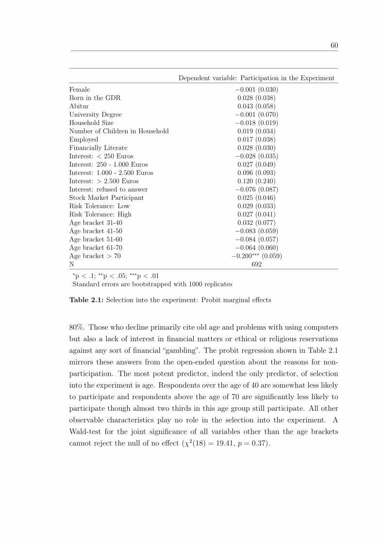
60

Dependent variable: Participation in the Experiment

Female −0.001 (0.030)Born in the GDR 0.028 (0.038)Abitur 0.043 (0.058)University Degree −0.001 (0.070)Household Size −0.018 (0.019)Number of Children in Household 0.019 (0.034)Employed 0.017 (0.038)Financially Literate 0.028 (0.030)Interest: < 250 Euros −0.028 (0.035)Interest: 250 - 1.000 Euros 0.027 (0.049)Interest: 1.000 - 2.500 Euros 0.096 (0.093)Interest: > 2.500 Euros 0.120 (0.240)Interest: refused to answer −0.076 (0.087)Stock Market Participant 0.025 (0.046)Risk Tolerance: Low 0.029 (0.033)Risk Tolerance: High 0.027 (0.041)Age bracket 31-40 0.032 (0.077)Age bracket 41-50 −0.083 (0.059)Age bracket 51-60 −0.084 (0.057)Age bracket 61-70 −0.064 (0.060)Age bracket > 70 −0.200∗∗∗ (0.059)N 692∗p < .1; ∗∗p < .05; ∗∗∗p < .01Standard errors are bootstrapped with 1000 replicates

Table 2.1: Selection into the experiment: Probit marginal effects

80%. Those who decline primarily cite old age and problems with using computersbut also a lack of interest in financial matters or ethical or religious reservationsagainst any sort of financial “gambling”. The probit regression shown in Table 2.1mirrors these answers from the open-ended question about the reasons for non-participation. The most potent predictor, indeed the only predictor, of selectioninto the experiment is age. Respondents over the age of 40 are somewhat less likelyto participate and respondents above the age of 70 are significantly less likely toparticipate though almost two thirds in this age group still participate. All otherobservable characteristics play no role in the selection into the experiment. AWald-test for the joint significance of all variables other than the age bracketscannot reject the null of no effect (χ2(18) = 19.41, p = 0.37).

61

2.1.2 Laboratory Experiment

Upon completion of the field data collection in the SOEP-IS, we used the iden-tical experimental module for a set of 198 university students in the WZB-TUBerlin decision laboratory. Recruitment into the laboratory sample followed stan-dard procedures.21 The instructions and sequence of informational displays onthe computer screens in the laboratory were as close to the CAPI environment aswe could produce them, so that the potential practical difficulties with the formatwould affect both populations. The experimental participants’ payments were alsoscaled by the same factor as payments to SOEP participants. The only relevantdifference in experimental design and procedures are that (i) the experimental par-ticipants do not have to fill out the long SOEP questionnaire, and (ii) we conductedonly two treatments with return shifters -10 and 10, in the laboratory, focusing onthe strongest treatment difference in incentives. Since the SOEP respondents whohappened to be in either of these two treatments were only informed about the ex-istence of these two treatments, we could leave the instructions entirely unchangedbetween survey and lab environments.

2.2 Experimental Data

2.2.1 Beliefs and Investments

We start with a summary description of investments and elicited beliefs. We willcall the share of wealth a respondent invests in the fund “equity share” hereafter.In both samples the distributions of equity shares have relatively wide supportsand few people invest all or nothing. Summing over all treatments, the means(and standard deviations in parentheses) of the equity share are 0.37 (0.25) inthe SOEP sample and 0.46 (0.31) in the laboratory sample. The proportions ofrespondents investing all, exactly half, or nothing in the risky asset are 0.03, 0.2and 0.18 in the SOEP sample and 0.12, 0.05 and 0.09 in the laboratory sample.

A description of the beliefs about the fund’s return is more involved, since eachbelief report consists of an entire histogram. A clear difference between the SOEP

21 The decision laboratory uses ORSEE (Greiner, 2015).

62

Equity ShareImputed

Expectationof Belief

Imputed S.D.of Belief

StatedExpectation

of BeliefMean S.D Mean S.D Mean S.D Mean S.D N

Overall 0.37 (0.25) 12.53 (20.59) 23.96 (16.54) 8.27 (17.84) 562

Age Bracket<30 0.41 (0.27) 12.16 (16.06) 30.25 (16.07) 8.74 (16.64) 8231-40 0.39 (0.22) 13.85 (15.73) 25.60 (17.13) 12.02 (16.54) 7641-50 0.40 (0.23) 12.57 (24.70) 26.36 (16.75) 7.12 (18.65) 10751-60 0.37 (0.26) 13.24 (21.86) 22.72 (16.46) 8.43 (19.41) 10761-70 0.34 (0.26) 10.02 (19.63) 20.46 (15.88) 6.22 (17.27) 111>70 0.32 (0.28) 14.13 (22.49) 19.19 (14.77) 8.36 (17.63) 79

Genderfemale 0.35 (0.24) 9.72 (22.29) 25.60 (17.20) 7.86 (21.59) 271male 0.39 (0.26) 15.14 (18.52) 22.43 (15.78) 8.65 (13.46) 291

Born inWest Germany 0.37 (0.26) 12.11 (20.97) 23.34 (15.60) 7.40 (17.38) 379East Germany 0.34 (0.23) 12.87 (21.96) 22.47 (17.46) 7.75 (17.69) 116abroad 0.42 (0.28) 14.95 (15.44) 29.74 (19.10) 14.66 (17.35) 54

Abituryes 0.37 (0.28) 10.74 (19.51) 26.70 (14.83) 6.40 (13.47) 122no 0.37 (0.25) 13.02 (20.87) 23.20 (16.93) 8.78 (18.85) 440

University Educationyes 0.35 (0.28) 11.54 (21.78) 26.95 (15.40) 5.55 (16.46) 72no 0.37 (0.25) 12.67 (20.42) 23.52 (16.67) 8.67 (18.01) 490

Employedyes 0.39 (0.25) 13.64 (20.70) 24.38 (16.13) 8.98 (16.13) 297no 0.35 (0.26) 11.27 (20.42) 23.49 (17.01) 7.47 (19.58) 265

Financially Literateyes 0.36 (0.25) 14.13 (20.80) 24.02 (15.98) 8.08 (17.68) 283no 0.38 (0.26) 11.05 (20.27) 24.00 (17.14) 8.47 (18.09) 277

Stock Owneryes 0.45 (0.29) 12.79 (18.20) 22.66 (14.55) 8.95 (13.82) 107no 0.35 (0.24) 12.50 (21.13) 24.29 (16.99) 8.11 (18.69) 454

“Financially Literate” is an indicator variable which is 1 whenever the respondent states that he/she is either “good” or “very good”with financial matters. For details on this and the other variables, see Appendix 2.A8.

Table 2.2: Experimental Responses in the SOEP by subgroup

63

and the lab is that the laboratory participants use more bins than the representa-tive respondents.22 The median number of bins that contain at least one brick is6 in the laboratory while it is only 3 in the SOEP where 28% of respondents useonly a single bin and a further 14% only use two bins.23

In the analysis below we repeatedly use summary statistics that we computefrom the reported histograms. To compute statistics like the expectation or thestandard deviation of returns from the underlying belief distribution we take the8 points on the CDF, interpolate between them using a cubic spline and thencalculate the statistics numerically.24 Using these imputed distributions, we findthat the average of the SOEP respondents’ mean expected return of the fundis 12.5% and the average standard deviation of the fund’s return distribution is24.0%. For the laboratory sample, the average mean belief about the fund’s returnis 11.6% and the average standard deviation is 35.6%.

As described in the previous section, we also elicited scalar belief reports byasking for the “expected” fund return. In the SOEP sample, this variable has amean of 8.3% and a standard deviation of 17.8%. In the laboratory sample, themean is 11.0% and the standard deviation is 19.1%. Stated expectations are highlycorrelated with expectations inferred from belief distributions (Pearson correlationcoefficient: 0.5 for the SOEP and 0.31 for the lab sample). Table 2.2 collects keydescriptives for the main experimental variables for different subgroups of theSOEP sample (a similar table for the lab sample is omitted because the studentpopulation is very demographically homogeneous).

We now investigate the extent to which equity share and beliefs are correlated.Figure 2.1 contains a scatter plot of equity shares and the belief measures for boththe SOEP and the lab sample. The figure shows pronounced positive relationshipsbetween belief and investment overall. At the mean of the data an increase in theexpected return by one percentage point is associated with a one third percentagepoint increase in the equity share (see Table 2.A3 in the Appendix for OLS re-

22 Appendix 2.A6 contains examples of the raw data of elicited histograms from both samples.23 Relative to comparable studies that use similar methods, the mentioned frequencies are on

the low side. Delavande and Rohwedder (2008) report that 73% of their subjects used two orfewer bins.

24 This method is due to Bellemare, Bissonnette, and Kröger (2012). A more detailed descriptionof the interpolation procedure can be found in Appendix 2.A7.

64

gressions). This relationship holds for both our belief measures and is roughly thesame in the laboratory. This evidence of a positive association between beliefs andinvestments is consistent with many studies in the belief elicitation literature (see,for example, Naef and Schupp (2009) and Costa-Gomes, Huck, and Weizsäcker(2014) in the context of trust games).

SOEPLab

SOEP Lab

0.00

0.25

0.50

0.75

1.00

-90 -60 -30 0 30 60 90 120Imputed Expectation

Equ

itySh

are

0.00

0.25

0.50

0.75

1.00

-90 -60 -30 0 30 60 90 120Imputed Expectation

Equ

itySh

are

0.00

0.25

0.50

0.75

1.00

-90 -60 -30 0 30 60 90 120Stated Expectation

Equ

itySh

are

0.00

0.25

0.50

0.75

1.00

-90 -60 -30 0 30 60 90 120Stated Expectation

Equ

itySh

are

Overlapping observations are aggregated, with the dot’s size being proportional to the number of observations thus aggregated.Model fit comes from a polynomial regression in which investments are a cubic function of expected return (Models 2, 5, 8 and 10in Table 2.A3 in the Appendix, which also contains alternative specification that e.g. control for personal characteristics but allshow results that are qualitatively and quantitatively similar.). 95% confidence interval in light gray.

Figure 2.1: Equity Share and Beliefs

Notice that the data also show patterns that are hard to square with the predic-tions of the standard model. As in Merkle and Weber (2014) there is a substantialfraction of participants who expect a negative excess return for the experimentalasset and yet invest positive amounts. But altogether, the statistical connectionbetween belief data and investment decisions can be regarded as supporting thebasic implication of the standard portfolio choice model: higher expected returnsoccur together with larger investments.

65

Stock-market partici-pation rate by...

Decile

1st 2nd 3th 4th 5th 6th 7th 8th 9th 10th

Household Income 7% 7% 3% 21% 14% 17% 20% 19% 26% 46%Liquid Wealth 0% 2% 2% 2% 5% 13% 11% 39% 43% 56%

Table 2.3: Stock-market participation rate by income and wealth deciles

2.3 External validity: Stock market participation

We now turn to the important question whether our response variables are in-dicative of real-life investments. Specifically, we test the external validity of ourdata by comparing elicited behavior in the experiment with survey responses to thequestion “Do you own any stock market mutual funds, stocks or reverse convertiblebonds (“Aktienanleihen”)?”

18% of all households answered this question in the affirmative, which is inline with other evidence on the German stock market participation.25 Splittingthe participation rate by deciles of both household income and a proxy for liquidwealth26 Table 2.3 also shows that stock market participation increases in bothvariables but stays well below 100%.

Figure 2.2 displays a correlogram, a visualization of the correlation matrix forseveral survey and experimental variables. Starting from the vertical, positivecorrelations are displayed as wedges that are shaded clockwise while negative cor-relations are shaded counter-clockwise. The higher the correlation, the larger thewedge and the darker the shade of the wedge.

The correlogram shows that only a handful of variables are reliable predictors ofstock market participation. Most of the significant correlations have been observedin the previous literature. For example, household size is known to be a significant

25 Most other surveys provide numbers only for the percentage of individuals who hold stocks.In our data this percentage stands at 15.4% (S.E.: 1.1%) while a 2012 survey by DeutschesAktieninstitut (2012) puts it at 13.7%.

26 The SOEP question about interest earned on investments over the previous year is answeredby far more people than more detailed questions about the amounts of wealth held in the formof various assets. We therefore use this variable as a proxy for liquid wealth. The alternativemeasure, the sum over all asset classes, yields broadly similar results. For details on thesevariables, see Appendix 2.A8.

66

StockOwner

HHIncome

EquityShare

Female

Age

Abitur

HHSize

RiskTolerance

E(DAX)

SD(DAX)

P(DAX>0)

The correlogram above visualizes the pairwise (Pearson) correlation coefficients of the variables.E(DAX) is the imputed expected return on the DAX going forward while SD(DAX) is the imputed standard deviation of thereported return distribution. P(DAX>0) is the reported probability that the DAX will make a gain over the next year.

Figure 2.2: Correlogram

correlate of stock market holdings. Likewise, household income and Abitur—thehighest form of secondary education in Germany and the only form that grantsaccess to the university system—are well-known and entirely unsurprising predic-tors of stock ownership. Notice that equity share is the only experimental variablethat has predictive power for stock holdings (correlation: 0.14, p-value: < 0.001).

Of course, the correlograms only show bivariate relations. In order to gaina broader picture we investigate whether the correlations change if we controlfor other variables.27 We find that equity share has explanatory power over and

27 This is similar to the approach taken by Guiso et al. (2008) who study the co-variation of stock

67

above the other variables, see Table 2.4. Even after including all relevant controls,which drives up the R2 to around 30%, the coefficient for equity share remainsboth economically important and statistically significant and is robust to differ-ent specifications. Back-of-the-envelope calculations yield the result mentioned inthe introduction, that an increase in equity share by one standard deviation isassociated with an increase in stock market participation of six percentage points.

The fact that equity share helps to explain stock holdings even if we control for allother variables that are known to be good predictors of stock market participationis important for two reasons. First, it establishes external validity. Investmentbehavior in the experiment is strongly related to investment behavior outside of theexperiment. Second, the result gives hope that the simple experimental portfoliochoice problem can be used as a wind tunnel: it allows the controlled manipulationof a behavioral variable that has a close connection to stock market particpation,both in terms of economic theory and in terms of empirical correlation. Hence,there is hope that interventions, for example, to encourage stock ownership, couldbe pre-tested in laboratory or artefactual field experiments such as ours.

market participation with generalized trust and other variables.

68

Dependent variable: Stock Market Participant

(1) (2) (3)

Equity Share 0.220∗∗∗ 0.240∗∗∗ 0.200∗∗∗(0.072) (0.068) (0.064)

Female −0.043 −0.029(0.032) (0.030)

Born in East Germany −0.058∗ −0.044(0.034) (0.033)

Age 0.006 0.004(0.005) (0.006)

Age2 −0.0001 −0.0001(0.0001) (0.0001)

Abitur 0.200∗∗∗ 0.150∗∗(0.061) (0.058)

University Degree 0.049 −0.003(0.078) (0.072)

Household Size 0.039∗∗ −0.004(0.019) (0.022)

Risk Tolerance: Low 0.020 0.034(0.037) (0.035)

Risk Tolerance: High 0.008 0.058(0.044) (0.043)

Imputed expectation of DAX 0.001 0.0003(0.001) (0.001)

Imputed S.D. of DAX −0.003∗∗∗ −0.001(0.001) (0.001)

Gain Probability of DAX −0.003 0.039(0.088) (0.085)

Number of Children in Household −0.096∗∗∗ −0.057∗(0.030) (0.030)

Employed −0.015 −0.024(0.036) (0.037)

Financially Literate 0.140∗∗∗ 0.080∗∗∗(0.032) (0.031)

Interest: < 250 Euros 0.061∗(0.033)

Interest: 250 - 1.000 Euros 0.270∗∗∗(0.057)

Interest: 1.000 - 2.500 Euros 0.430∗∗∗(0.086)

Interest: > 2.500 Euros 0.310∗∗∗(0.110)

Interest: refused to answer 0.150(0.100)

Household Income (missing=0) 0.023(0.018)

Household Income: missing 0.210∗∗(0.084)

Constant 0.110∗∗∗ −0.130 −0.130(0.029) (0.140) (0.140)

N 561 560 560R2 0.021 0.150 0.280Adjusted R2 0.019 0.130 0.250∗p < .1; ∗∗p < .05; ∗∗∗p < .01Household income is in thousands of Euros

Household income is set to zero where missing (48 cases). Moreover, a dummy variable is added to the regression which is 1 forthe observations with missing household income.

Table 2.4: Predicting real-world stock-market participation

69

2.4 Treatment effects

Recall that we implement five exogenous treatments that shift the historical returnof the DAX. The shifts are sizable, ranging from -10 percentage points to +10percentage points. Table 2.5 documents that by and large there is, surprisingly,no effect of the return shifter on equity share in the SOEP sample. The lack ofresponse can hardly be explained by small incentives. In terms of the nominalframing of the e50,000 investment, the difference in returns between Treatments-10 and 10 amounts to a difference in returns of up to e10,000. In terms of the realmonetary value of the experimental investment, the variation in return amounts toa difference of up to e5. This difference is large enough for the typical participantin an experiment (even in representative samples) to react. The overall lack ofresponse therefore suggests that many respondents find it difficult to incorporatethe shift appropriately in their investment choice.

However, this result is not universal. Instead we notice an important differencebetween the SOEP and the laboratory sample. While SOEP participants appear toignore the shifter on average, there is a strong and statistically significant reactionof investments to the treatment in the laboratory. There, the equity share risesfrom 0.30 to 0.63 in response to improving the return of the fund by 20 percentagepoints.

Similar results hold for those parts of the SOEP sample that are plausibly morefinancially savvy, those who are more educated, those who have more liquid assets(or refuse to answer the question about how much interest they obtain from liq-uid assets) and those who answer the standard financial literacy question aboutcompound interest correctly. Hence, it appears that the main difference betweenSOEP and lab is driven by selection on educational covariates and wealth.28

The beliefs about the fund’s return, however, do not respond to the shifter inthe way they should, no matter what measure of beliefs we use and no matterwhether we consider the SOEP data or the laboratory data and no matter howwe slice the data. While there is a statistically significant effect in the laboratorysample, it is much smaller than the 20 percentage points predicted by probabilistic

28 For details of differences between subsamples, see Appendix 2.A3.

70

Setting Variable -10 -5 0 5 10 ANOVA Kruskall-Wallis

SOEP Equity Share 0.40 (0.02) 0.34 (0.02) 0.32 (0.02) 0.39 (0.02) 0.39 (0.02) 0.106 0.135Imputed Beliefs 13.14 (1.97) 10.58 (1.81) 9.38 (1.85) 14.48 (1.83) 14.45 (2.18) 0.232 0.326Stated Beliefs 8.55 (1.71) 7.68 (1.70) 6.60 (1.98) 9.28 (1.43) 8.93 (1.66) 0.810 0.990Probability of a Gain 0.68 (0.03) 0.67 (0.03) 0.67 (0.03) 0.74 (0.02) 0.69 (0.03) 0.323 0.313

Lab Equity Share 0.30 (0.03) 0.63 (0.03) 0.000 0.000Imputed Beliefs 10.05 (1.71) 13.37 (1.57) 0.156 0.016Stated Beliefs 9.87 (2.28) 12.30 (1.38) 0.374 0.004Probability of a Gain 0.59 (0.02) 0.65 (0.01) 0.029 0.009

Table 2.5: Mean levels by treatment

sophistication, and there is no effect at all in the SOEP sample. In both samplesand regardless of whether we consider imputed beliefs or stated beliefs, we canstrongly reject the rational prediction that the shifter moves the mean of beliefsone-to-one.

We tentatively conclude from this evidence that it is much harder to manipulatebeliefs than to elicit them. As we show in Appendix 2.A1 subjects’ beliefs aboutpast DAX returns are surprisingly accurate. Within each of the seven histogrambins, the population-average belief of DAX returns falling in the bin is within justfew percentage points of the historical frequency. But just like the investments,the beliefs do not react strongly enough to the experimental manipulation. Thisalso raises the question how well the respondents understand the manipulation,despite our long and intense efforts for clarity in the instructions. The next sectioninvestigates the possibility that the weak reaction to the manipuation may bedriven by factors beyond the understanding of the experimental instructions.

2.5 Asset Complexity and Reactions to Changes in

Incentives

In this section we investigate the role of complexity with an additional laboratoryexperiment. We introduce manipulations of both the risky asset and the safeasset that are economically equivalent and described in identical terms. Yet, theexperiment shows that the reaction to an increase in the risky asset’s return isweaker than the reaction to an increase in the safe asset’s return. This effect islargely consistent with the available evidence on reactions to tax incentives as,e.g., in Chetty et al. (2009) and Abeler and Jäger (2015).

71

In the additional experiment, the excess return of the risky asset is varied intwo ways: either a shift of ∆ in the risky asset’s return, or a shift of −∆ in thesafe asset’s return. To make the two shifts economically equivalent, we modifythe decision maker’s exogenous income level, as detailed in the next subsection.However, before proceeding to the details, two remarks are in order: First, wedesigned this section’s experiment after we observed the results from the exper-iments described in Section 2.1.2—hence the separate presentation. Second, thefact that we could run the complexity experiment only in a laboratory format alsomeans that we cannot investigate the present research question for the subsamplesthat show the weakest reaction to incentive shifts. We suspect, but have no proof,that these subsamples would exhibit even larger differences in their reactions todifferent shifts.

2.5.1 Experimental Design

The design follows the same format as the paper’s main experiment, implementingthe standard portfolio choice problem. In the new experiment (i) each participantmakes eight investment decisions, allowing a within-subject analysis, and (ii) eachparticipant receives a task-specific fixed income in addition to the earnings fromthe portfolio choice.

The participants are endowed with an illiquid asset that generates the fixedincome WI , and with liquid wealth WL that they can allocate among a safe assetand a risky asset. The risky asset pays a rate of return r whereas the safe assetpays a rate of return rf .

Now consider an increase in the risky return r by an amount ∆, analogous tothe exogenous return manipulation of the paper’s main experiment. Under thismanipulation, a decision maker who invests α in the risky asset earns a randompayoff given by:

π(α) = αWL(1 + r +∆) + (1− α)WL(1 + rf ) +WI

For a framing variation of this manipulation by ∆, we can alternatively inducea simultaneous shift in rf by amount −∆ and in WI by amount ∆WL, yieldingthe same payoff from investing a share α in the risky asset:

72

π(α) = αWL(1 + r) + (1− α)WL(1 + rf −∆) + (WI +∆WL)

From the fact that π(α) is identical between both treatments and for all α,we conclude that the same risks are available between the two manipulations.Consequently, expected utility theory, and any other theory that employs a stablemapping from a constant set of uncertainty states into the risky asset’s returnrate, predict an identical choice by the decision maker. The same statement istrue if both the safe and the risky assets’ returns are additionally shifted by aconstant amount ∆′. The experiment’s null hypothesis is thus that participantsreact equally between the equivalent manipulations of incentives applying to thesafe asset or the risky asset.

To ensure that the results are not driven by an asymmetry between positiveshifts and negative shifts, we formulate the entire experiment such that only pos-itive shifts occur. This is achieved by adding an appropriate return shift ∆′ toboth assets.29 The parameters for the eight choice problems are displayed in Ta-ble 2.7. The collection of equivalent variations is the following: Problems 1 and 3are economically equivalent, Problems 2 and 4 are economically equivalent, Prob-lems 5 and 7 are economically equivalent, and Problems 6 and 8 are economicallyequivalent. Problems 1 and 2 differ only in the risky asset’s return; Problems 3and 4 differ in the shifter applied to the riskless asset (and a compensatory changein the illiquid endowment), in the described way. But the difference in incentivesis the same between 1 and 2 as between 3 and 4. Thus, expected utility and mostof its generalizations predict that the difference in investments is identical. Analo-gously, the difference between 5 and 6 is predicted to be identical to the differencein investments between 7 and 8. As described above, our main hypothesis in thisexperiment is that shifts in safe return generate a stronger reaction: investments

29 We also ran three pilot sessions but do not use the data gathered in these sessions here. Inthe first pilot session subjects were presented with both “bonuses” and “fees” on the two assetsand displayed aversive reactions to any asset to which a fee was applied. Since the effect ofgain/loss framing was not the subject of this study we therefore ran two sessions with bonusesonly but found that up to 42% of subjects chose investments at the lower boundary of thebudget set. Since this much truncation presents problems both in terms of power and in termsof the distributional assumptions one is required to make to deal with it, we therefore changedthe magnitude of the bonuses to arrive at the valued reported here, values that yield muchfewer truncated responses. Note, however, that the responses in all pilots were also indicativeof stronger reactions to changes in the safe asset.

73

Treatment Bonus onRisky Asset

Bonus on Risk-less Asset

Illiquid En-dowment

Liquid Endow-ment

1 9.00 5.90 16000 500002 2.65 5.90 16000 500003 5.90 2.80 17550 500004 5.90 9.15 14375 500005 9.10 6.05 14275 500006 3.10 6.05 17275 500007 6.05 3.00 15800 500008 6.05 9.00 15800 50000

Table 2.7: Treatment parameters

may differ more between 3 and 4 than between 1 and 2, and more between 7 and8 than between 5 and 6.

76 participants were recruited into 4 experimental sessions at WZB-TU Berlinlaboratory in the spring of 2014, using identical procedures as in the study de-scribed in Section 2.1.2. Similar to the first lab study we take a fixed-interestGerman government bond (here, yielding 2 % per annum) as the safe asset andthe return on the DAX in a year randomly drawn from 1951 to 2010 as the riskyasset. Treatments were presented in random order so as to avoid confounds fromlearning or contrast effects. One of the eight tasks was randomly selected and paidout at the end of the experiment, ensuring incentive compatibility for each task.

2.5.2 Results

Figure 2.3 displays the differences in average equity shares (the percentage of theliquid endowment invested in the risky asset) for each of the four treatment pairs.A weaker reaction to changes in the risky asset return is immediately visible.Treatments 1 and 2 vary the risky asset return by 6.35 percentage points whileholding the riskless asset return constant. This causes a change in mean equityshare from 0.28 when the bonus on the risky asset is 2.65 percentage points to 0.62when the bonus on the risky asset is 9 percentage points for a difference of 0.34.A change of equal magnitude in the return of the riskless asset causes a larger

74

0.25

0.30

0.35

0.40

0.45

1 – 2Change in

Risky Asset Shifter

3 – 4Change in

Riskless Asset Shifter

5 – 6Change in

Risky Asset Shifter

7 – 8Change in

Riskless Asset Shifter

Diff

eren

cein

Equ

itySh

ares

Error bars show 95% confidence intervals.

Figure 2.3: Investments in the risky asset by treatment

change in the equity share. While the mean equity share in treatment 3 is 0.61,almost identical to that in treatment 1, the mean equity share in treatment 4 is0.21, lower than that in treatment 2. This yields a difference of 0.4. The samepattern of responses hold analogously for treatments 5 to 8.30

Given the comparatively small sample size, each of these mean responses is sub-ject to considerable sampling error. In order to formally test our main hypothesiswe therefore pool the data from all treatments. We compute the difference indifferences for treatments 1 to 4 and add to this the difference in differences fortreatments 5 to 8. Under the null of rational, equal-sized responses to changes ineither the risky and riskless asset returns this sum should be zero. Instead, we findit to be 0.10, positive and statistically significantly so (two-sided Wilcoxon ranksum test p-value = 0.03, two-sided t-test p-value = 0.09).31

30 A graph of the raw responses is available in Appendix 2.A10.31 Over all treatments about 11% of responses are truncated below at zero. The percentage of

75

2.6 Conclusion

The paper at hand describes a simple portfolio choice problem with one safe andone risky asset, implemented in an artefactual field experiment for a representa-tive population sample in Germany. The data from this experiment exhibit highdegrees of external validity as shown through direct comparison of behavior insideand outside the experiment. This may be viewed as a success for the standardportfolio choice model. Despite its extreme reductionism it captures importantreal-life tradeoffs in financial markets.

The analysis also shows that the degree of external validity varies between dif-ferent subgroups. External validity is stronger for skilled and savvy subjects. Wealso observe that only these savvier subgroups of subjects respond in a meaningfulway to changes in incentives, highlighting, once again, the important role of cogni-tive ability for even the simplest financial decision problems (Benjamin, Brown, &Shapiro, 2013). In our setting less educated subjects forgo substantial additionalearnings by not responding to exogenous shifts in investment incentives. Relatedto previous studies on financial literacy (e.g. Lusardi and Mitchell (2011) on re-tirement savings, Gerardi, Goette, and Meier (2013) on mortgage foreclosure andvon Gaudecker (2015) on portfolio diversification), this difference addresses thepossibility of distributional effects that arise from cognitive differences. Similarinterventions to foster investments in real life (such as tax subsidies for equityholdings) could have similar undesired effects.

In a separate experiment, we also find evidence that asset complexity is a fac-tor in this under-reaction to incentives. Even university students, who comparefavorably with the general population on proxies for cognitive ability, react morestrongly to shifts in the return of an asset with a constant return than to shifts inan asset with a stochastic return when both shifts are economically equivalent. Toour knowledge, this is a phenomenon that has not yet been documented in the liter-ature on financial literacy, with the exception of the related effects in Chetty et al.(2009) and Abeler and Jäger (2015). This phenomenon—performance in addition

truncated responses is higher in treatments 4 and 8 than it is in treatments 2 and 6. Thetruncation therefore potentially obscures larger differences between treatments 3 and 4, and 7and 8, and biases the differences the test statistic towards zero.

76

can be depend on the nature of the variable to which a number is added—raisesquestions for the psychology of arithmetic (Ashcraft, 1992) and has potentially nu-merous applications in the realm of economic decision making under uncertainty.

For future research, our study may inform the design of further wind tunnelsfor interventions regarding financial investment of households. In particular, inthe light of the current underfunding of many pension systems (both pay as yougo and capital funded), greater stock market participation by the middle classappears desirable to many economists and policy makers. Testing interventions inartefactual field experiments such as ours might avoid costly mistakes.

77

2.7 References

Abdellaoui, M., Baillon, A., Placido, L. L., & Wakker, P. P. (2010). The rich do-main of uncertainty: source functions and their experimental implementation.The American Economic Review, 101 (April), 695–723.

Abeler, J. & Jäger, S. (2015). Complex tax incentives. American Economic Jour-nal: Economic Policy, 7 (3), 1–28.

Allen, F. (1987). Discovering personal probabilities when utility functions are un-known. Management Science, 33 (4), 542–544.

Andersen, S., Harrison, G., Lau, M., & Rutström, E. (2008). Eliciting Risk andTime Preferences. Econometrica, 76 (3), 583–618.

Armantier, O. & Treich, N. (2013). Eliciting Beliefs: Proper Scoring Rules, Incen-tives, Stakes and Hedging. European Economic Review, 62, 17–40.

Arrondel, L., Calvo-Pardo, H., & Tas, D. (2012). Subjective Return Expectations,Information and Stock Market Participation: Evidence from France.

Ashcraft, M. H. (1992). Cognitive arithmetic: A review of data and theory. Cog-nition, 44 (1-2), 75–106.

Bellemare, C., Bissonnette, L., & Kröger, S. (2012). Flexible Approximation ofSubjective Expectations Using Probability Questions. Journal of Business& Economic Statistics, 30 (1), 125–131.

Benjamin, D. J., Brown, S. A., & Shapiro, J. M. (2013). Who is ‘Behavioral’?Cognitive Ability and Anomalous Preferences. Journal of the European Eco-nomic Association, 11 (6), 1231–1255.

Bertrand, M., Karlan, D., Mullainathan, S., Shafir, E., & Zinman, J. (2010).What’s Advertising Content Worth? Evidence from a Consumer Credit Mar-keting Field Experiment. Quarterly Journal of Economics, 125 (1), 263–306.

Binswanger, J. & Salm, M. (2013). Does Everyone Use Probabilities? Intuitive andRational Decisions about Stockholding (IZA Discussion Papers No. 7265).Institute for the Study of Labor (IZA).

Bucher-Koenen, T. & Lusardi, A. (2011). Financial Literacy and Retirement Plan-ning in Germany (Working Paper No. 17110). National Bureau of EconomicResearch.

78

Campbell, J. Y. & Viceira, L. M. (2002). Strategic Asset Allocation: PortfolioChoice for Long-term Investors. New York: Oxford University Press.

Chetty, R., Looney, A., & Kroft, K. (2009). Salience and taxation: theory andevidence. American Economic Review, 99 (4), 1145–1177.

Choi, S., Kariv, S., Müller, W., & Silverman, D. (2014). Who Is (More) Rational?American Economic Review, 104 (6), 1518–1550.

Costa-Gomes, M., Huck, S., & Weizsäcker, G. (2014). Beliefs and actions in thetrust game: Creating instrumental variables to estimate the causal effect.Games and Economic Behavior, 88, 298–309.

Delavande, A., Giné, X., & McKenzie, D. (2011). Eliciting probabilistic expecta-tions with visual aids in developing countries: how sensitive are answers tovariations in elicitation design? Journal of Applied Econometrics, 497 (3),479–497.

Delavande, A. & Rohwedder, S. (2008). Eliciting subjective probabilities in internetsurveys. Public Opinion Quarterly, 72 (5), 866–891.

Deutsches Aktieninstitut. (2012). Zahl der Aktienbesitzer geht wieder zurück. DeutschesAktieninstitut. Frankfurt am Main.

Dimmock, S. G., Kouwenberg, R., Mitchell, O. S., & Peijnenburg, K. (2013). Ambi-guity Aversion and Household Portfolio Choice: Empirical Evidence. NBERWorking Paper, (18743).

Dohmen, T., Falk, A., Huffman, D., Sunde, U., Schupp, J., & Wagner, G. G.(2011). Individual risk attitudes : measurement, determinants and behavioralconsequences. Journal of the European Economic Association, 9 (3), 522–550.

Dominitz, J. & Manski, C. F. (2011). Measuring and interpreting expectations ofequity returns. Journal of Applied Econometrics, 26, 352–370.

Dominitz, J. & Manski, C. F. (2007). Expected Equity Returns and PortfolioChoice: Evidence from the Health and Retirement Study. Journal of theEuropean Economic Association, 5 (2-3), 369–379.

Forsythe, G. E., Malcolm, M. A., & Moler, C. B. (1977). Computer Methods forMathematical Computations. Englewood Cliffs, NJ: Prentice-Hall.

Fox, C. R. & Tversky, A. (1995). Ambiguity Aversion and Comparative Ignorance.Quarterly Journal of Economics, 45 (1), 97–113.

79

Gerardi, K., Goette, L., & Meier, S. (2013). Numerical ability predicts mortgagedefault. Proceedings of the National Academy of Sciences of the United Statesof America, 110 (28), 11267–71.

Goldstein, D. G. & Rothschild, D. (2014). Lay Understanding of Probability Dis-tributions. Judgment and Decision Making, 9 (1), 1–14.

Greiner, B. (2015). Subject pool recruitment procedures: organizing experimentswith ORSEE. Journal of the Economic Science Association, 1 (1), 114–125.

Grinblatt, M., Keloharju, M., & Linnainmaa, J. (2011). IQ and Stock MarketParticipation. Journal of Finance, 66 (6), 2121–2164.

Guiso, L., Sapienza, P., & Zingales, L. (2008). Trusting the stock market. Journalof Finance, 63 (6), 2557–2600.

Haliassos, M. & Bertaut, C. C. (1995). Why Do So Few Hold Stocks. EconomicJournal, 105 (September), 1110–1129.

Huck, S. & Müller, W. (2012). Allais for all: Revisiting the Paradox in a LargeRepresentative Sample. Journal of Risk and Uncertainty, 44 (3), 261–293.

Huck, S. & Weizsäcker, G. (1999). Risk, complexity, and deviations from expected-value maximization: results of a lottery choice experiment. Journal of Eco-nomic Psychology, 20, 699–715.

Hurd, M. D. & Rohwedder, S. (2012). Stock Price Expectations and Stock Trading.NBER Working Paper, (17973).

Hurd, M. D., van Rooij, M., & Winter, J. (2011). Stock market expectations ofdutch households. Journal of Applied Econometrics, 26, 416–436.

Hyman, J. (1983). Accurate Monotonicity Preserving Cubic Interpolation. SIAMJournal on Scientific and Statistical Computing, 4 (4), 645–654.

Karni, E. & Safra, Z. (1995). The Impossibility of Experimental Elicitation ofSubjective Probabilities. Theory and Decision, 38, 313–320.

Kézdi, G. & Willis, R. J. (2009). Stock market expectations and portfolio choice ofamerican households.

Lusardi, A. & Mitchell, O. S. (2011). Financial Literacy and Planning: Implicationsfor Retirement Wellbeing (Working Paper No. 17078). National Bureau ofEconomic Research.

80

Merkle, C. & Weber, M. (2014). Do investors put their money where their mouthis? stock market expectations and investing behavior. Journal of Banking &Finance, 46, 372–386.

Merton, R. (1969). Lifetime Portfolio Selection under Uncertainty: The Continuous-Time Case. Review of Economics and Statistics, 51 (3), 247–257.

Naef, M. & Schupp, J. (2009). Measuring Trust: Experiments and Surveys in Con-trast and Combination (IZA Discussion Papers No. 4087). Institute for theStudy of Labor (IZA).

Rabin, M. & Weizsäcker, G. (2009). Narrow Bracketing and Dominated Choices.American Economic Review, 99 (4), 1508–1543.

Richter, D. & Schupp, J. (2012). SOEP Innovation Sample (SOEP-IS) — Descrip-tion and Structure of the SOEP Innovation Sample. SOEPpapers, (463).

Rothschild, D. (2012). Expectations: Point-Estimates, Probability Distributions,Confidence, and Forecasts.

Samuelson, P. (1969). Lifetime Portfolio Selection by Dynamic Stochastic Pro-gramming. Review of Economics and Statistics, 51 (3), 239–246.

Stehle, R., Huber, R., & Maier, J. (1996). Rückberechnung des DAX für die Jahre1955 bis 1987.

Stehle, R., Wulff, C., & Richter, Y. (1999). Die Rendite deutscher Aktien in derNachkriegszeit - DAX-Rückberechnung für die Jahre 1948 bis 1955.

Trautmann, S. T. & van de Kuilen, G. (2015). Belief Elicitation: A Horse Raceamong Truth Serums. Economic Journal, 125 (589), 2116–2135.

van Rooij, M., Lusardi, A., & Alessie, R. (2007). Financial Literacy and Stock Mar-ket Participation (Working Paper No. 13565). National Bureau of EconomicResearch.

Vissing-Jorgensen, A. (2004). Perspectives on Behavioral Finance: Does "Irra-tionality"Disappear with Wealth? Evidence from Expectations and Actions.NBER Macroeconomics Annual 2003, 18.

von Gaudecker, H. M., van Soest, A., & Wengström, E. (2011). Heterogeneity inRisky Choice Behavior in a Broad Population. American Economic Review,101, 664–694.

81

von Gaudecker, H.-M. (2015). How Does Household Portfolio Diversification Varywith Financial Literacy and Financial Advice? Journal of Finance, 70 (2),489–507.

Wilcox, N. T. (1993). Lottery choice: incentives, complexity and decision time.Economic Journal, 103 (421), 1397–1417.

82

2.8 Appendices

2.A1 Calibration

SOEPLab

SOEP Lab

-----

-

----

-

---

-

-

----

-

----

----------

0.0

0.1

0.2

0.3

0.4

0.5

(-90%

,-60%

]

(-60%

,-30%

]

(-30%

,0%]

(0%,30

%]

(30%,60

%]

(60%,90

%]

(90%,12

0%]

Return Bin

Pro

babi

lity

- -

-

-

-

-

-

-

-

-

- - --

0.0

0.1

0.2

0.3

0.4

0.5

(-90%

,-60%

]

(-60%

,-30%

]

(-30%

,0%]

(0%,30

%]

(30%,60

%]

(60%,90

%]

(90%,12

0%]

Return Bin

Pro

babi

lity

Shifter-10

-5

0

5

10

Historical benchmark for each treatment indicated by black horizontal lines.

Figure 2.A1: Historical distribution of returns vs. the average distributions in Lab andSOEP

Figure 2.A1 compares the respondents’ beliefs about the fund’s return with thetrue historical distribution of DAX returns. The figure shows, in different shades ofgray and ordered from left to right within each bin, the five different distributionsof beliefs for the five different treatments. The figure also compares these distri-butions with five corresponding true distributions, indicated by black horizontallines for each bin and treatment, that result from the true historical distributionplus the five shifters (in the same order, that is, from -10 to the very left to +10to the very right, within each bin). The figure shows that SOEP respondents areremarkably well calibrated. In none of the seven bins are respondents off by more

83

than 5 percentage points when data are pooled across treatments. The largest twodeviations are that the frequency of small losses between 0 and 30% is slightlyunderestimated and the frequency of larger losses is slightly overestimated. Thegood calibration can also be seen in other metrics. While the mean return on theDAX from 1951 to 2010 was 15.5%, both the imputed and the stated expected re-turn on the experimental asset of 12.5% and 8.3% respectively—while lower—areat least similar in magnitude to the historical mean. Moreover, while the relativefrequency of a positive return over these six decades was 70.0%, SOEP respondentsthought the DAX had seen a gain 69.3% of the time.32 In contrast, the averagedistribution of our student subjects in the lab (also shown in Figure 2.A1) differssignificantly from the historical benchmark in that too much probability mass isassumed to be in the tails of the distribution.

Underneath the excellent calibration of the average SOEP respondent’s belieflies, however, substantial heterogeneity in beliefs and miscalibration at the indi-vidual level. Very few of the distributions provided by individual respondents areclose to the historical benchmark, and what produces the excellent calibration inthe aggregate is a mixture of respondents who put the entire probability mass intoa single bin and respondents who report diffuse distributions.

That the return expectations we elicit show such remarkable calibration standsin contrast to evidence from other countries, where substantial miscalibration iscommonly observed. For the US Kézdi and Willis (2009) report that HRS re-spondents expected a stock market gain with roughly 50% probability in the 2002,2004 and 2006 waves while the historical frequency of a gain on the Dow Joneswas 68%. Similarly, the probability of a gain larger than 10% was estimated at39% but the corresponding frequency was 49%. Dominitz and Manski (2011) findsimilar numbers in the monthly surveys of the Michigan Survey of Consumers frommid-2002 to mid-2004. In the Netherlands, Hurd et al. (2011) find that in 2004the median expected rate of return on the Dutch stock market index was a mere

32 In order to predict whether subjects invest in the risky asset, a relevant question—underexpected utility, the only relevant question—is whether respondents expect a strictly positiveexcess return, i.e. a mean return that exceeds 4%. Based on reported beliefs, the proportionof respondents who expect a strictly positive excess return is 69.2% when using stated beliefs,and 72.6% when using imputed beliefs. The historical frequency of the DAX returning strictlymore than 4% is 68.3%.

84

Expectations of fund’s past performanceSOEP Lab

0.0

0.2

0.4

0.6P

roba

bilit

y

Expectations of DAX’s next-year performanceSOEP Lab

0.0

0.2

0.4

0.6

(-90%

,-60%

]

(-60%

,-30%

]

(-30%

,0%]

(0%,30

%]

(30%,60

%]

(60%,90

%]

(90%,12

0%]

(-90%

,-60%

]

(-60%

,-30%

]

(-30%

,0%]

(0%,30

%]

(30%,60

%]

(60%,90

%]

(90%,12

0%]

Pro

babi

lity

Error bars are 95% confidence interval.

Figure 2.A2: Average distributions of past and future returns

0.3%, a severe underestimate of the historical median return of 14%. A downwardbias in expectations is by no means a universal finding, however. Respondents inthe 1999, 2000 and 2001 waves of the Survey of Economic Expectations reportedexpectations for the S&P500 that were substantially above the historical average,but also held the S&P500 to be more volatile than has been the case historically(Dominitz & Manski, 2011).

What explains these differences with the existing literature? One possible expla-nation is that the papers quoted above compare respondents’ expectations aboutthe future with returns realized in the past. A test for correct calibration in thissetting then amounts to a joint test of whether subjects hold the historical distri-bution of returns to be identical to the distribution of returns in the future and,if so, whether they have an accurate picture of the historical distribution. In con-trast, we elicit beliefs about the distribution of returns over a well-defined periodof time in the past and can test for calibration without auxiliary assumptions.

85

The beliefs that we elicit about the next 12 months look, however, fairly similar, ifsomewhat more pessimistic – see Figure 2.A2. This may not be entirely surprisingas the survey period was just after the economic crises in parts of Europe hadreached their peak intensity. In contrast to expectations about the past, whereSOEP respondents and students differed substantially (with the former being morerealistic), we find virtually identical expectations about the future between the twosamples. The mean imputed return is 12.5% while the probability of a gain on theDAX is thought to be 58.8% on average. 51.8% of subjects state that they expecta return that is higher than 4%.

86

2.A2 Equity Share and Beliefs – Regressions

Dependent Variable: Equity ShareSOEP: Stated Beliefs SOEP: Imputed Beliefs Lab: Stated Beliefs Lab: Imputed Beliefs

(1) (2) (3) (4) (5) (6) (7) (8) (9) (10)

Imputed Expected Return 0.003∗∗∗ 0.005∗∗∗ 0.005∗∗∗ 0.003∗∗ 0.007∗∗∗

(0.0005) (0.001) (0.001) (0.001) (0.003)Imputed Expected Return2 −0.00002∗∗∗ −0.00001 −0.0001

(0.00001) (0.00001) (0.0001)Imputed Expected Return3 −0.00000∗∗ −0.00000∗∗∗ −0.00000

(0.00000) (0.00000) (0.00000)Imputed S.D. of Return 0.001

(0.001)Probability of a Gain −0.010

(0.037)Stated Expected Return 0.004∗∗∗ 0.005∗∗∗ 0.005∗∗∗ 0.002 0.006

(0.0005) (0.001) (0.001) (0.002) (0.005)Stated Expected Return2 −0.00001 −0.00001 −0.0001

(0.00001) (0.00001) (0.0002)Stated Expected Return3 −0.00000 −0.00000 0.00000

(0.00000) (0.00000) (0.00000)Constant 0.330∗∗∗ 0.330∗∗∗ 0.370∗∗∗ 0.340∗∗∗ 0.330∗∗∗ 0.400∗∗∗ 0.420∗∗∗ 0.410∗∗∗ 0.440∗∗∗ 0.420∗∗∗

(0.012) (0.013) (0.110) (0.011) (0.013) (0.110) (0.028) (0.035) (0.030) (0.037)Personal Controls No No No No No No No No No NoN 562 562 560 562 562 560 198 198 198 198R2 0.074 0.093 0.160 0.081 0.090 0.140 0.031 0.063 0.016 0.038Adjusted R2 0.072 0.088 0.120 0.080 0.085 0.100 0.026 0.048 0.011 0.023

∗p < .1; ∗∗p < .05; ∗∗∗p < .01Personal controls include dummy variables for gender, being born in the former GDR, having Abitur, having a university education, being employed,having a high self-assessed financial literacy, owning stocks and for each level of our wealth proxy. They also include age and age2, household size,the number of children in the household and household incomeAll standard errors are Huber-White heteroskedasticity-robust

Figure 2.A3: Equity Share and Beliefs

87

2.A3 Different results for different people

In this section we exploit the rich data set on the SOEP respondents in orderto study the role of socioeconomic background variables and direct measures orplausible correlates of savviness. As described in Section 2.4, we find strong differ-ences between the SOEP sample and the university student sample regarding theextent to which they react to incentives. This raises the question of whether thereis other evidence that “smart”, financially savvy respondents react more stronglyto variations in incentives. The following analysis confirms the existence of suchdifferences.

We caution that our examination of heterogeneity in the SOEP sample is a “fish-ing exercise”. However, its results are largely in line with what other studies havedocumented before, namely the fundamental role of cognitive ability for financialdecisions making.

Table 2.A2 documents treatment effects on choices and beliefs for different sub-groups. It shows that there are small subsamples of the population that do reactto incentives. For respondents with a university degree, the coefficients indicate anincrease in equity share of one percentage point per one percentage point increasein return. Moving from the worst shifter of -10 to the best shifter of +10, theequity share is predicted to increase by 20 percentage points. This is similar tothe effect we observe in the laboratory study with university students where theequity share increases by 33 percentage points. Hence, it appears that the maindifference between SOEP and lab is driven by selection on educational covariates.

The results for respondents with different wealth levels are somewhat mixed. Forreasons one can only speculate about, the strongest treatment effect is observed forthose who withhold information on income from interest. There is also a notablecomposition effect between the two largest categories: respondents with low butpositive levels of income from interest are predicted to increase their equity shareby 14 percentage points when we move from the worst to the best shifter. Thosewithout any interest earnings are estimated to exhibit a negative treatment effect.

Among the financial literacy questions we find a heterogeneous treatment effectonly for the compound interest question. The other variables that might capturefinancial literacy do not show significant interactions with the experimental treat-

88

ment. While the results on financial literacy and wealth are a bit patchy, overalla picture emerges that is familiar from the literature. Even relatively simple in-vestment tasks as the one we have implemented here appear to be cognitively socomplex that sensible responses to variations in parameters are shown only byskilled and sophisticated subjects.

An inspection of the two right-hand columns of Table 2.A2 reveals that whenit comes to belief manipulation no systematic patterns emerge. Only one of theinteractions is statistically significantly different from zero, but only marginally so.

Given that we can identify some subgroups that react better to incentives, it isnot far-fetched to presume that we might also be able to detect a stronger externalvalidity of investment levels for these groups. With less noise in behavior insideand presumably outside the laboratory, the measured correlations between theexperimental equity share and stock market participation may increase. Table 2.A1shows the regression-based conditional correlates of stock market participation,separately for different subgroups. Indeed it is the case that “smarter” subsamplesshow stronger external validity.

89

Stock Market ParticipantAll Abitur University Degree Financially Literate

Equity Share 0.200∗∗∗ 0.370∗∗ 0.480 0.230∗∗(0.064) (0.180) (0.300) (0.110)

Female −0.029 −0.120 −0.230 −0.049(0.030) (0.110) (0.150) (0.052)

Born in East Germany −0.044 −0.021 −0.160 −0.083(0.033) (0.120) (0.190) (0.061)

Age 0.004 −0.028 −0.062 0.002(0.006) (0.023) (0.044) (0.011)

Age2 −0.0001 0.0003 0.001 −0.00004(0.0001) (0.0002) (0.0005) (0.0001)

Abitur 0.150∗∗ 0.240∗∗(0.058) (0.100)

University Degree −0.003 −0.002 −0.041(0.072) (0.097) (0.120)

Household Size −0.004 0.036 0.045 −0.020(0.022) (0.087) (0.110) (0.035)

Risk Tolerance: Low 0.034 −0.015 −0.0003 0.048(0.035) (0.110) (0.140) (0.059)

Risk Tolerance: High 0.058 −0.002 0.098 0.058(0.043) (0.160) (0.240) (0.064)

Imputed expectation of DAX 0.0003 0.002 0.001 0.001(0.001) (0.007) (0.010) (0.003)

S.D. of DAX −0.001 −0.002 0.002 −0.001(0.001) (0.004) (0.005) (0.002)

Gain Probability of DAX 0.039 −0.051 −0.330 0.062(0.085) (0.310) (0.480) (0.160)

Number of Children in Household −0.057∗ −0.110 −0.180 −0.062(0.030) (0.110) (0.150) (0.049)

Employed −0.024 0.033 0.022 −0.007(0.037) (0.120) (0.210) (0.067)

Financially Literate 0.080∗∗∗ 0.170∗ 0.200(0.031) (0.100) (0.150)

Interest: < 250 Euros 0.061∗ 0.047 −0.033 0.086(0.033) (0.110) (0.170) (0.054)

Interest: 250 - 1.000 Euros 0.270∗∗∗ 0.330∗∗ 0.270 0.320∗∗∗(0.057) (0.140) (0.220) (0.084)

Interest: 1.000 - 2.500 Euros 0.430∗∗∗ 0.560∗∗∗ 0.560∗∗ 0.440∗∗∗(0.086) (0.180) (0.240) (0.110)

Interest: > 2.500 Euros 0.310∗∗∗ 0.150 0.013 0.560∗∗∗(0.110) (0.170) (0.300) (0.170)

Interest: refused to answer 0.150 0.350 0.046 0.260(0.100) (0.250) (0.360) (0.170)

Household Income (missing=0) 0.023 0.039 0.029 0.010(0.018) (0.040) (0.059) (0.029)

Household Income: missing 0.210∗∗ 0.150 0.520 0.140(0.084) (0.330) (0.560) (0.130)

Constant −0.130 0.580 1.400 −0.007(0.140) (0.490) (0.910) (0.260)

N 560 122 72 283R2 0.280 0.360 0.480 0.320Adjusted R2 0.250 0.220 0.260 0.260∗p < .1; ∗∗p < .05; ∗∗∗p < .01

Standard errors are Huber-White heteroskedasticity-robust. Household income is set to zero where missing (48 cases). Moreover, adummy variable is added to the regression which is 1 for the observations with missing household income. “Financially Literate” isan indicator variable which is 1 whenever the respondent states that he/she is either “good” or “very good” with financial matters.For details on this and the other variables, see Appendix 2.A8.

Table 2.A1: Stock market participation by subgroups

90

Equity Share Imputed Expectation ofFund

Stated Expectation of Fund

Mean Treatment Effect Mean Treatment Effect Mean Treatment Effect

Education< University Degree 0.373 (0.011) 0.000 (0.002) 12.646 (0.922) 0.107 (0.139) 8.649 (0.815) 0.076 (0.113)University Degree 0.349 (0.033) 0.010∗∗ (0.004) 11.426 (2.619) 0.325 (0.353) 5.586 (2.039) -0.115 (0.300)

Interest from Wealth0 0.368 (0.017) -0.005∗∗ (0.002) 13.265 (1.572) 0.110 (0.224) 9.012 (1.597) 0.086 (0.214)< 250 Euros 0.360 (0.019) 0.007∗∗∗ (0.003) 10.576 (1.344) 0.320 (0.207) 7.759 (1.113) 0.076 (0.163)250 - 1.000 Euros 0.344 (0.027) 0.001 (0.004) 18.231 (1.758) -0.123 (0.297) 9.618 (1.569) -0.247 (0.301)1.000 - 2.500 Euros 0.422 (0.048) -0.005 (0.007) 13.582 (3.266) 0.501 (0.518) 7.783 (1.846) 0.011 (0.204)> 2.500 Euros 0.382 (0.054) 0.004 (0.007) 7.830 (8.722) -0.653 (1.246) 5.481 (3.307) 0.206 (0.246)refused to answer 0.339 (0.073) 0.015∗∗ (0.007) 1.971 (8.978) 0.558 (1.030) 3.353 (3.572) 0.543 (0.351)

Financial Literacy: self-assessed’good’ or ’very good’ 0.360 (0.015) 0.002 (0.002) 14.064 (1.231) 0.287 (0.180) 8.047 (1.059) 0.153 (0.153)’a little’ or ’not at all’ 0.381 (0.016) -0.001 (0.002) 11.052 (1.227) -0.001 (0.183) 8.479 (1.091) -0.056 (0.147)

Financial Literacy: compound interestcorrect 0.384 (0.014) 0.004∗ (0.002) 13.066 (1.157) 0.177 (0.178) 8.741 (0.865) 0.080 (0.117)incorrect 0.349 (0.018) -0.003 (0.003) 11.381 (1.415) 0.119 (0.190) 7.701 (1.431) 0.004 (0.213)don’t know 0.365 (0.059) -0.003 (0.006) 15.608 (3.751) -0.161 (0.547) 8.560 (4.725) 0.005 (0.533)

Financial Literacy: volatilitycorrect 0.400 (0.047) -0.005 (0.007) 21.056 (4.591) -0.415 (0.664) 14.726 (4.607) -0.763 (0.640)incorrect 0.372 (0.012) 0.001 (0.002) 11.938 (0.906) 0.161 (0.134) 7.911 (0.755) 0.084 (0.102)don’t know 0.301 (0.041) 0.003 (0.006) 11.234 (3.342) 0.556 (0.439) 4.944 (3.744) 0.980∗ (0.561)

Stock Owneryes 0.448 (0.028) -0.002 (0.004) 12.828 (1.756) -0.054 (0.308) 9.280 (1.417) -0.439∗ (0.237)no 0.353 (0.011) 0.002 (0.002) 12.483 (0.992) 0.185 (0.142) 8.099 (0.878) 0.157 (0.118)

The table shows the results of multivariate regressions in which, for each set of rows, the outcome variables in the columns are regressed on indicator variables for the different levelsof the row variables and a variable for the size of the shifter interacted with the different levels of the row variables. “Mean” and “Treatment Effect” therefore correspond to theconstants and slope coefficients in bivariate regressions of the column variables on each of the different levels of the row variables. Standard errors for OLS regressions are Huber-Whiteheteroskedasticity-robust.

Table 2.A2: Treatment effect by subgroups

91

2.A4 Histogram Belief Elicitation Screen

Figure 2.A4: Belief elicitation screen

92

2.A5 Descriptive Statistics

Statistic N Mean St. Dev. Min Max

Female 700 0.480 0.500 0 1Age 700 53.000 17.000 16 94Born in Germany 700 0.860 0.350 0 1Born in the GDR 700 0.200 0.400 0 1Abitur 700 0.200 0.400 0 1University degree 700 0.120 0.330 0 1Employed 700 0.500 0.500 0 1Household Size 700 2.300 1.200 1 8Number of Children in Household 700 0.360 0.780 0 6Monthly Household Income (in 1000s of Euros) 652 2.500 1.500 0.100 12.000Risk Tolerance 700 4.900 2.500 0 10Financial Literacy (self-assessed: ’good’ or ’very good’) 697 0.500 0.500 0 1Financial Literacy (compound interest question correct) 690 0.580 0.490 0 1Financial Literacy (volatility question correct) 690 0.840 0.370 0 1Equity share (in experiment) 562 0.370 0.260 0.000 1.000Imputed expectation of fund 562 13.000 21.000 −80.000 110.000Stated expectation of fund 562 8.300 18.000 −80.000 95.000Gain Probability of Fund 562 0.690 0.280 0.000 1.000Imputed expectation of DAX 562 5.500 18.000 −60.000 90.000Gain Probability of DAX 562 0.590 0.330 0.000 1.000Total Liquid Assets 515 19.000 44.000 0.000 446.000Stock Market Participation 693 0.180 0.390 0 1Stocks (amount) 671 1,780.000 7,874.000 0 110,000Stocks / Total Liquid Assets 452 0.066 0.190 0.000 1.000Total Debt 666 17,174.000 54,514.000 0 800,000

N is the number of non-missing observations

Table 2.A3: Descriptive statistics for the 700 heads of household in SOEP sample

93

2.A6 Some Individual Belief Distributions

SOEPLab

SOEP Lab

0.000.250.500.751.00

0.000.250.500.751.00

0.000.250.500.751.00

0.000.250.500.751.00

0.000.250.500.751.00

0.000.250.500.751.00

0.000.250.500.751.00

0.000.250.500.751.00

(-90%

,-60%

](-6

0%,-3

0%]

(-30%

,0%

](0

%,3

0%]

(30%

,60%

](6

0%,9

0%]

(90%

,120

%]

(-90%

,-60%

](-6

0%,-3

0%]

(-30%

,0%

](0

%,3

0%]

(30%

,60%

](6

0%,9

0%]

(90%

,120

%]

(-90%

,-60%

](-6

0%,-3

0%]

(-30%

,0%

](0

%,3

0%]

(30%

,60%

](6

0%,9

0%]

(90%

,120

%]

Return Bin

Pro

babi

lity

0.000.250.500.751.00

0.000.250.500.751.00

0.000.250.500.751.00

0.000.250.500.751.00

0.000.250.500.751.00

0.000.250.500.751.00

0.000.250.500.751.00

0.000.250.500.751.00

(-90%

,-60%

](-6

0%,-3

0%]

(-30%

,0%

](0

%,3

0%]

(30%

,60%

](6

0%,9

0%]

(90%

,120

%]

(-90%

,-60%

](-6

0%,-3

0%]

(-30%

,0%

](0

%,3

0%]

(30%

,60%

](6

0%,9

0%]

(90%

,120

%]

(-90%

,-60%

](-6

0%,-3

0%]

(-30%

,0%

](0

%,3

0%]

(30%

,60%

](6

0%,9

0%]

(90%

,120

%]

Return Bin

Pro

babi

lity

Figure 2.A5: 24 randomly chosen belief distributions from both the SOEP and the labsample.

94

2.A7 Imputation of Moments

To derive various summary statistics from the elicited belief distributions we fitcontinuous distributions to the raw data and calculate the statistics from thesedistributions.

While much of the existing literature fits parametric distributions we follow anapproach similar to Bellemare et al. (2012) and fit cubic interpolating splines usingan approach due to Forsythe, Malcolm, and Moler (1977). We first cumulate theprobabilities that respondents place within each of the seven bins. This yields8 points on the cumulative distribution function from which the responses weregenerated. We take these 8 points to be the knots of the spline (that is, we ignoreany rounding in the response and assume that the CDF at these points is known)and interpolate between them with a piecewise cubic polynomial.

Since each of the 7 pieces is defined by four polynomial coefficients this is aproblem with 28 unknowns. The condition that the spline must go through eachof the 8 points gives 14 equations (one each for the end-points and two eachfor the interior knots) and further assuming that the spline is twice continuouslydifferentiable at each of the knots yields 12 additional equations. What pins downthe spline are two boundary conditions, which are found by fitting exact cubicsthrough the four points closest to each boundary and imposing the third derivativesof these cubics at the end-points on the spline.

What is problematic about using such a spline to impute a CDF is that nothingin the procedure described above guarantees that the resulting spline is monotonic.To overcome this problem we apply a filter to the spline that is due to Hyman(1983). The filter relaxes some of the smoothness conditions enough to ensuremonotonicity.33

Figure 2.A6 demonstrates the fit for six representative respondents. Circlesshow the raw cumulative probabilities to which both the Hyman-filtered cubicsplines as well as various alternative distributions are fitted. By construction thesplines are extremely close to the data in all cases – often much closer than anyof the parametric distributions that have been fit to the data by minimizing the

33 Both the Forsythe et al. construction of the spline as well as the Hyman filter are implementedin R through the splinefun() function with methods fmm and hyman respectively

95

● ●

●

●

●

●

● ●

−90% −30% 30% 90%

0

0.25

0.5

0.75

1

● ● ● ●

● ● ● ●

−90% −30% 30% 90%

0

0.25

0.5

0.75

1

● ● ●

● ●

● ● ●

−90% −30% 30% 90%

0

0.25

0.5

0.75

1

● ●

●

●

●

● ● ●

−90% −30% 30% 90%

0

0.25

0.5

0.75

1

● ● ●

●

● ● ● ●

−90% −30% 30% 90%

0

0.25

0.5

0.75

1

● ●

●

● ●

●

● ●

−90% −30% 30% 90%

0

0.25

0.5

0.75

1

Hyman−filtered cubic spline

linear spline

log−normal distribution

gamma distribution

Figure 2.A6: CDFs derived from the belief data using both spline interpolation andparametric distributions fit via least squares

sum of squared deviations at the 8 points. The two distributions on the left aresingle-peaked and have non-zero probability in several bins and for these cases allof the methods yield roughly the same fit. The distributions in the middle havemass only in a single or in two of the bins, which is a problem for the parametricdistributions because in such cases the fit can be improved ad infinitum by reducingthe variance of the distribution and thereby reducing the sum of squared deviationsat the 8 points. In the two cases on the right the distribution is multi-modal,which naturally leads to terrible fit for the parametric distributions, all of whichare unimodal. The splines, in contrast make no such assumptions and thereforefit even these cases rather well.

Finally, we calculate both the mean and the standard deviation from thesedistributions numerically using adaptive Gauss-Kronrod quadrature.

96

2.A8 Variable Description and Coding

The full data set contains 1146 respondents in 700 households. Since asset allo-cation is commonly seen in the literature as the result of joint optimization of allhousehold members we narrow the sample to the 700 heads of household, whichwe identify as the respondents who filled out the SOEP household questionnaire.All demographics whose coding is detailed below are the demographics of thishousehold head.

Abitur

Germany has a multi-track educational system in which only students who gradu-ate from high school with an “Abitur” diploma are automatically allowed to enrollat university. In the SOEP respondents are asked directly for the highest sec-ondary school degree they have obtained and our Abitur variable is coded mainlyaccording to the answer to this question. There is one special case, however, thatrequires special attention. 59 respondents obtained their secondary education out-side of Germany and a separate question gives too little information to be able tomap the secondary education they obtained into the German educational systemprecisely. Of these subjects, 11 have university degrees, however; education forwhich, had it been obtained in Germany, the Abitur would almost always be aprerequisite. Since we are interested in the Abitur as a proxy for higher abilityand higher education and foreign respondents with university degrees plausiblyposses the same higher ability and higher education we recode these subjects ashaving Abitur.

Born in East Germany

This indicator variable is 1 if the respondent was born in the German DemocraticRepublic. It is 0 for respondents born in the Federal Republic of Germany, thoseborn outside of Germany and those born in East Germany after reunification in1990 (14 cases).

97

Interest from Wealth

This variable is our main proxy for respondents’ liquid wealth holdings. Thoughour survey module included detailed questions about more specific asset classes,item non-response rates for the questions asking for the invested amounts werefairly high. The household questionnaire also included the question “How large, allin all, was your income from interest, dividend payments and capital gains in 2011”,with six answer categories.34 For the econometric analysis we generate a variablethat uses information from both questions. We create a new category for subjectswho report that their capital income was precisely zero, sort all respondents whogave exact answers into the six categories above and then merged the highest threecategories into a single category for capital incomes above e2500 to increase thecell count (counts before the merge were 20 for the e2500 to e5000 category, 5 forthe e5000 to e10000 category and 5 for the more than e10000 category). Lastly,we added a category for all subjects who refused to answer both questions.

Financial Literacy

We assess respondents’ financial literacy in two different ways. First, we ask peopleto self-assess their financial literacy with the question:

“How good, all in all, are you with financial matters?”35

• very good• good• a little• not at all

Second, we ask two questions that explicitly test respondents’ financial literacy:

“Suppose you have e100 in a savings account. You receive 20% onthis amount per year and leave the money in the account for 5 years.

34 In German: “Wie hoch waren, alles in allem, die Einnahmen aus Zinsen, Dividenden undGewinnen aus allen Ihren Wertanlagen im Jahr 2011?”. Many respondents were either unwillingor unable to provide a precise answer to this question. In a follow-up question they weretherefore asked to estimate the amount and choose between 6 categories: below e250, e250to e1000, e1000 to e2500, e2500 to e5000, e5000 to e10000, more than e10000

35 In German: “Wie gut kennen Sie sich alles in allem in finanziellen Angelegenheiten aus? Garnicht, ein bisschen, gut oder sehr gut?”

98

How much money will be in the account after these 5 years?”36.• more than e200• exactly e200• less than e200• don’t want to answer

“Which of the following types of investments has the largest fluctua-tions in returns over time?”37.

• savings accounts• fixed income securities• stocks• don’t want to answer

Liquid assets

All household members are asked about individual holdings of the following assettypes:

1. checking accounts2. savings accounts3. call deposit accounts (“Tagesgeld”)4. fixed deposits5. covered bonds, municipal bonds, bank bonds, corporate bonds or sovereign

bonds6. stock market mutual funds, stocks or reverse convertible bonds (“Aktienan-

leihen”)7. real estate funds8. bond and money market funds9. other funds

10. other securitiesFor each of these types, respondents are first asked whether they own any assets ofthat type at all and, if the question is answered affirmatively, about the size of the36 In German: “Angenommen, Sie haben 100 eGuthaben auf Ihrem Sparkonto. Dieses Guthaben

wird mit 20% pro Jahr verzinst, und Sie lassen es 5 Jahre auf diesem Konto. Wie viel Guthabenweist Ihr Sparkonto nach 5 Jahren auf?”

37 In German: “Was glauben Sie: Welche der folgenden Anlageformen zeigt im Laufe der Zeit diehöchsten Ertragsschwankungen? Sparbücher, festverzinsliche Wertpapiere oder Aktien?”

99

asset holdings. Respondents are instructed to estimate this amount should theybe unable to provide an exact figure. We code a household as participating in thestock market if the head of household answers the question about stock marketmutual funds, individual stocks and reverse convertible bonds with “yes”.

100

101

2.A9 Predicting real-world stock-market participation –

alternative wealth measures and specifications

Dependent Variable: Stock Market ParticipantOLS OLS OLS OLS OLS Probit marginal effects

(1) (2) (3) (4) (5) (6)

Equity Share 0.220∗∗∗ 0.240∗∗∗ 0.200∗∗∗ 0.210∗∗∗ 0.140∗ 0.170∗∗∗

(0.072) (0.068) (0.064) (0.066) (0.076) (0.056)Female −0.043 −0.029 −0.028 −0.028 −0.016

(0.032) (0.030) (0.030) (0.033) (0.029)Born in East Germany −0.058∗ −0.044 −0.032 −0.021 −0.079∗∗

(0.034) (0.033) (0.032) (0.036) (0.036)Age 0.006 0.004 0.002 0.006 0.003

(0.005) (0.006) (0.005) (0.006) (0.006)Age2 −0.0001 −0.0001 −0.00004 −0.0001 0.000

(0.0001) (0.0001) (0.0001) (0.0001) (0.000)Abitur 0.200∗∗∗ 0.150∗∗ 0.140∗∗ 0.120∗ 0.140∗∗∗

(0.061) (0.058) (0.058) (0.065) (0.044)University Degree 0.049 −0.003 0.013 −0.014 −0.021

(0.078) (0.072) (0.074) (0.083) (0.052)Household Size 0.039∗∗ −0.004 0.003 0.013 0.003

(0.019) (0.022) (0.023) (0.028) (0.019)Risk Tolerance: Low 0.020 0.034 0.033 0.020 0.017

(0.037) (0.035) (0.035) (0.039) (0.033)Risk Tolerance: High 0.008 0.058 0.052 0.058 0.068

(0.044) (0.043) (0.043) (0.048) (0.042)Imputed expectation of DAX 0.001 0.0003 0.0005 −0.0002 0.001

(0.001) (0.001) (0.001) (0.001) (0.002)S.D. of DAX −0.003∗∗∗ −0.001 −0.002∗∗ −0.001 −0.002∗∗

(0.001) (0.001) (0.001) (0.001) (0.001)Gain Probability of DAX −0.003 0.039 0.035 0.096 0.003

(0.088) (0.085) (0.081) (0.096) (0.083)Number of Children in Household −0.096∗∗∗ −0.057∗ −0.067∗∗ −0.072∗∗ −0.092∗∗∗

(0.030) (0.030) (0.031) (0.035) (0.031)Employed −0.015 −0.024 −0.030 −0.006 −0.015

(0.036) (0.037) (0.037) (0.042) (0.039)Financially Literate 0.140∗∗∗ 0.080∗∗∗ 0.091∗∗∗ 0.078∗∗ 0.071∗∗

(0.032) (0.031) (0.032) (0.036) (0.030)Interest: < 250 Euros 0.061∗ 0.120∗∗∗

(0.033) (0.046)Interest: 250 - 1.000 Euros 0.270∗∗∗ 0.260∗∗∗

(0.057) (0.047)Interest: 1.000 - 2.500 Euros 0.430∗∗∗ 0.330∗∗∗

(0.086) (0.058)Interest: > 2.500 Euros 0.310∗∗∗ 0.270∗∗∗

(0.110) (0.069)Interest: refused to answer 0.150 0.170∗

(0.100) (0.090)Total Liquid Assets (missing=0) 0.011∗∗∗

(0.003)Total Liquid Assets2 (missing=0) −0.0001∗∗

(0.00003)Total Liquid Assets3 (missing=0) 0.00000

(0.00000)Total Liquid Assets: missing 0.130∗∗∗

(0.040)Household Income (missing=0) 0.023 0.032∗ 0.020∗

(0.018) (0.017) (0.012)Household Income: missing 0.210∗∗ 0.230∗∗∗ 0.180∗∗∗

(0.084) (0.082) (0.069)Total Liquid Assets 0.012∗∗∗

(0.003)Total Liquid Assets2 −0.0001∗∗

(0.00003)Total Liquid Assets3 0.00000

(0.00000)Household Income 0.020

(0.019)Constant 0.110∗∗∗ −0.130 −0.130 −0.100 −0.210

(0.029) (0.140) (0.140) (0.130) (0.140)N 561 560 560 560 417 560R2 0.021 0.150 0.280 0.290 0.310

∗p < .1; ∗∗p < .05; ∗∗∗p < .01Income and Liquid assets are in thousands of Euros. Standard errors for OLS regressions are Huber-Whiteheteroskedasticity-robust. Standard errors for probit marginal effects are bootstrapped with 1000 replicates

102

2.A10 Raw Data in Complexity Experiment

0.0

0.5

1.0

1 2 3 4 5 6 7 8

Equ

itySh

are

6.059.10 6.053.109.00 2.65 5.905.90

3.006.05 9.006.055.90 5.90 9.152.80

15800.0014275.00 15800.0017275.0016000.00 16000.00 14375.0017550.00

Bonus onRisky Asset

Bonus onRiskless Asset

Illiquid Endowment

Treatment

Point size is proportional to the number of overlapping observations.

Figure 2.A7: Raw Data in Complexity Experiment

3 Measuring Ambiguity Aversion: Experimental

Tests of Subjective Expected Utility

based on work with James Andreoni & Charles Sprenger

3.1 Introduction

Many of the most important economic decisions are made in environments inwhich no appeal can be made to objective probabilities. In areas such as portfolioallocation, healthcare and insurance coverage, the likelihood of decision-relevantevents is not externally “given” but must be judged by the decision maker herself.Subjective Expected Utility (SEU) provides an elegant representation of choicein such contexts (Anscombe & Aumann, 1963; Savage, 1954). Under SEU, adecision maker acts as if she maximizes the expectation of the utility outcomesof her choice with the expectation governed by a coherent subjective probabilitymeasure.1 The Savage development and critical contributions of the Anscombeand Aumann (1963) framework have made SEU a benchmark model of choicethroughout economics.

Subjective Expected Utility came under scrutiny from its origination.2 Notably,the Ellsberg (1961) urn paradoxes drew attention sharply towards potential SEUviolations.

Ellsberg’s two color problem presents two urns,1 That is, the subjective probability of each event is in the interval [0, 1], the probability ofthe union of disjoint event is the sum of their probabilities, and the entire state space hasprobability 1

2 Interestingly, for decision-making with objective probabilities, the famous Allais (1953) para-doxes were distributed at the same conference as Savage’s presentation of the Sure-ThingPrinciple (Savage, 1953) and Samuelson’s presentation of Independence (Samuelson, 1953) inMay of 1952.

103

104

• Urn A: 100 red and black balls in unknown proportion• Urn K: 50 red balls and 50 black balls,

and requests consideration of the following four choices:

1. Bet red A or Bet black A2. Bet red K or Bet black K3. Bet red K or Bet red A4. Bet black K or Bet black A.A bet on Urn A is a bet on a subjective event, while a bet on Urn K is a bet on

an objective event. A likely choice pattern is indifference in (1) and (2), and strictpreference for bets on Urn K in (3) and (4). This violates SEU as there exists noprobability measure which can rationalize choice.3 Originally stated as a thoughtexperiment the Ellsberg two color problem, and variants thereof, have since beendemonstrated in laboratory experiments (see Camerer & Weber, 1992, for a sur-vey of the early experimental evidence). Subjective Expected Utility requires aconsistency of behavior across subjective event bets that is clearly violated in thedata.

Important theoretical contributions have sought to relax the requirement ofconsistent subjective probabilities. One clarifying development is presented byGilboa and Schmeidler (1989) who consider decision makers who, when faced withambiguity, behave as if they did not attribute a single probability measure to anevent, but rather consider a set of probabilities and maximize expected utilitywith respect to the least favorable probability measure from the set. Such a “max-min" decisionmaker can easily display the inconsistency shown in the two colorproblem. At the most extreme, the decisionmaker is permitted to entertain thepessimistic notions that all the balls in Urn A are black when choosing betweenthe bets in (3) and that all balls in Urn A are red when choosing between the betsin (4). Additional models have been developed with more nuanced objectives of3 Under SEU a decision maker strictly prefers a bet on red from Urn K to a bet on red fromUrn A iff he believes the probability of drawing a red ball from Urn K to be higher than theprobability of drawing a red ball from Urn A. He prefers a bet on black from Urn K to a beton black from Urn A iff he believes the probability of drawing a black ball from Urn K to behigher than the probability of drawing a black ball from Urn A. Since drawing a red ball anddrawing a black ball are complementary events, by additivity and unitarity their probabilitiesmust add to one and so the latter implies that the probability of drawing a red ball from UrnK must be lower than the probability of drawing a red ball from Urn A, which contradicts thebelief that rationalizes the first choice.

105

describing decisionmaking under ambiguity, chief among them the smooth modelof Klibanoff, Marinacci, and Mukerji (2005).

Our objective in the present study is to return to the consistency requirements ofthe SEU model in order to develop deeper insights into individual decisionmakingand potentially provide identification of competing non-SEU models. In additionto consistency à l’Ellsberg between two subjective events, Subjective-SubjectiveConsistency, we consider Subjective-Objective Consistency. Subjective-ObjectiveConsistency states that when considering mixtures between subjective and objec-tive bets, a decisionmaker must also behave as if a single probability measure gov-erned her choice.4 The distinction between Subjective-Subjective Consistency andSubjective-Objective Consistency is important for two reasons. First, of the twopopularized non-SEU models we discuss, both deliver Subjective-Subjective incon-sistencies while only that of Gilboa and Schmeidler (1989) maintains Subjective-Objective Consistency. Hence investigating Subjective-Objective Consistency al-lows for separation that a standard Ellsberg experiment cannot deliver. Second,though Ellsberg style experiments are frequent in the literature, questions testingSubjective-Objective Consistency have yet to be implemented experimentally.5

Particular forms of violations may lead to interesting insights on the structure ofdecision making when subjective ambiguity can be replaced with objective uncer-tainty.

We present a design predicated on testing Subjective-Subjective Consistencyand Subjective-Objective Consistency. Our design elicits precise valuations of sub-jective, objective, and mixed subjective-objective bets through a series of binarystatements. For example, subjects state whether they prefer a draw from a jar con-4 This consistency requirement is closely associated with what is known in the literature as theCertainty Independence axiom. While Anscombe-Aumann Independence requires that prefer-ences not depend on mixing the acts involved with any act, Certainty Independence requiresmerely that preferences be invariant to mixing with constant (objective) acts. Certainty In-dependence underlies a broad class of non-SEU models, most notably Gilboa and Schmeidler(1989) and Schmeidler (1989). For a full characterization of the class that shares this ax-iom, the class of invariant biseparable preferences, see Ghirardato, Maccheroni, and Marinacci(2004).

5 An early literature moved suggestively in this direction by examining situations of partialambiguity where individuals were told some portion of the distribution from which outcomeswould be drawn. These experiments have been infrequent, with some of the treatments inBecker and Brownson (1964), Curley and Yates (1985) and Hong, Bin, and Songfa (2013)being leading examples.

106

taining an ambiguous composition of 20 red and green marbles, wherein red pays$10 and green pays $30, or a draw from a jar of known composition containing 20yellow and black marbles, wherein yellow pays $0 and blacks pays $30. Variation inthe jar of known composition that induces a change in preference from the ambigu-ous jar to the known jar provides a measure of valuation. Note this is effectivelythe experimental implementation of the Schmeidler (1989) ‘risk equivalent’ and isthe natural extension to the subjective domain of eliciting a cardinal utility indexfor an objective lottery.6 Comparing valuations for two complementary subjectivebets allows identification of Subjective-Subjective Consistency à l’Ellsberg.7 Mix-tures of subjective and objective bets allow identification of Subjective-ObjectiveConsistency.8

In an experiment conducted with 133 subjects at the University of California,San Diego, we document substantial deviations for both of our consistency no-tions. 79% of subjects violate Subjective-Subjective Consistency largely in a man-ner reminiscent of Ellsberg’s two-color problem. The mean data place valuationsof an ambiguous jar 10% below that of a known 50-50 jar regardless of paymentlabels. Such behavior is rationalized in our data by estimates of beliefs indicatingsubjects believe an ambiguous jar is composed of around 70% low-paying mar-bles regardless of the color that pays the low outcome. Surprisingly, over 95% ofsubjects violate Subjective-Objective Consistency. The mean behavior indicatesa “directed pessimism," consistent with subjects believing that an ambiguous jarconsists of around 90% low-paying marbles when mixing with a known high out-come, while believing that the same ambiguous jar consists of only around 55%low-paying marbles when mixing with a known low outcome. Interestingly, thecorrelation between inconsistencies at the individual level is limited, suggestingpossible differentiation in individuals’ ambiguity attitudes and their treatment ofsituations in which subjective ambiguity is replaced with objective uncertainty.

6 A standard cardinal utility index constructed in proofs of von Neumann-Morgenstern expectedutility identifies the cardinal utility of a gamble as the mixture of the best and worst optionsin the space of outcomes that yields indifference. See, for example, Varian (1992).

7 That is, we compare the valuations of ambiguous urns with either red pays $10, green pays$30 or red pays $30, green pays $10 relative to a jar with known 50-50 composition.

8 For example, we examine the valuation of 10 ambiguous marbles and 10 red marbles with redpays $10, green pays $30 to the valuation of 10 ambiguous marbles and 10 green marbles withred pays $10, green pays $30. The operationalization is described in Section 3.3.

107

Our exploration of consistency yields several conclusions and insights for futurework. Our pattern of deviations is at odds with SEU as well as popularized non-SEU models. Our data, however, give instruction as to what modeling constructsmay prove useful in capturing behavior. Potential suggestions include mixturedependence for ambiguity attitude and explicit subjective bet considerations costs.Naturally, however, a full elaboration and foundation for such constructs is outsidethe scope of this work. Even without an articulated model, our findings mayprove useful for the investigation of other behaviors. We consider several potentialapplications related to the newer finding of Subjective-Objective inconsistency.

The paper proceeds as follows. Section 3.2 presents a conceptual frameworkfor our SEU consistency tests and briefly considers the predictions of alternativemodels. Section 3.3 describes the design and procedures. Section 3.4 presentsresults and Section 3.5 provides discussion and a conclusion.

3.2 Conceptual Framework

Our broad setting is that of Anscombe and Aumann (1963). There is a finite statespace, S, a set of consequences, X, a set of objective probability distributionsover these consequences, ∆(X), and a set of acts, F , functions which map S into∆(X).9 Individuals carry preferences, ≿, over acts in F .

If preferences over acts satisfy axioms of completeness, transitivity, monotonic-ity, independence, continuity and non-degeneracy, they can be represented by theSubjective Expected Utility (SEU) functional. For a given act, a,

USEU(a) =

∫S

p(s) u(a(s)) ds

where p(s) refers to the subjective probability associated with state s ∈ S,∫Sp(s)ds =

1 and u(a(s)) is the (von Neumann-Morgenstern) expected utility of the lotterythat act a yields in state s.9 This, rather than the original formulation by Savage (1954) in which states map directlyinto consequences, has become the canonical choice domain on which models of choice underuncertainty are formulated. Note that objective lotteries are primitives of the model allowingone to describe “roulette” lotteries with probabilities objectively given and “horse race” lotteriesfor which probabilities are wholly subjective.

108

With this foundation, we introduce an Ellsberg style jar composed of red andgreen marbles with the color of a drawn ball determining the state of the world.Hence, the state space is binary, S = {red, green}. We establish the set of conse-quences as X = {0, x, y} with 0 < x < y. We consider two simple subjective actsthat are complements:10

• f : yields y with probability 1 if s = red, yields x with probability 1 ifs = green.

• g: yields y with probability 1 if s = green, yields x with probability 1 ifs = red.

The act f represents a bet on the subjective event red, while the act g representsa bet on the subjective event green.

In order to elaborate our consistency tests it will be helpful to introduce twodegenerate objective acts:11

• h: yields y with probability 1 if s = red, yields y with probability 1 ifs = green.

• l: yields x with probability 1 if s = red, yields x with probability 1 ifs = green.

These acts yield the high prize, y, with probability 1 in both states, or the lowprize, x, with probability 1 in both states.

Our consistency implications are constructed from these four acts. The develop-ment is aided by recalling a key axiom used in the SEU construction, Independence.

Definition 1 (Independence). For any three acts a, b, c ∈ F and any α ∈ (0, 1)

a ≿ b ⇐⇒ αa+ (1− α)c ≿ αb+ (1− α)c. (3.1)

Independence states that the preference between two acts should not changewhen both acts are mixed with any other in equal proportion.12 Independencehelps ensure the SEU formulation is linear in subjective probabilities and that

10 By simple act we mean that the distribution over X, ∆(X), induced in each state is degenerate.In the literature these are also known as “Savage acts.”

11 That is, the acts are governed by objective probabilities and induce the same degeneratedistribution over X in every state.

12 Where mixtures are probabilistic mixtures which are performed state-wise. The mixture αa+(1− α)c denotes an act, which yields the lotteries αa(s) + (1− α)c(s) in every state s.

109

the probabilities indeed constitute a proper probability measure. Our consistencyimplications build closely from the requirements of a coherent probability measureand linearity in probabilities.

3.2.1 Subjective-Subjective Consistency

SEU implies the existence of coherent subjective probability measure between com-plementary subjective acts. That is, for acts f and g a single subjective probability,p̃green = 1 − p̃red, must rationalize the valuations for both f and g. Consider theacts f , g and 1

2h+ 1

2l, the acts corresponding to Ellsberg’s classic 2-color problem.

Under SEU these acts are associated with the expected utilities

USEU(f) = (1− p̃green) · u(y) + p̃green · u(x)

USEU(g) = p̃green · u(y) + (1− p̃green) · u(x)

USEU(1

2h+

1

2l) =

1

2· u(y) + 1

2· u(x)

We present Subjective-Subjective Consistency as the restriction on the valua-tions of f and g relative to the valuation of 1

2h + 1

2l. The term derives from the

restricted pattern of behavior between the subjective probabilities associated withf and g.

Subjective-Subjective Consistency: 12[USEU(f) + USEU(g)] = USEU(

12h+ 1

2l)

SEU requires that the average valuation of the subjective acts f and g be equalto the valuation of the objective act 1

2h+ 1

2l. The implication is clear from noting

that 12[USEU(f) + USEU(g)] = USEU(

12h + 1

2l) = 1

2· u(y) + 1

2· u(x). Most Ellsberg

style experiments examine and reject an implication of this consistency require-ment, namely that the valuations of f and g (weakly) lie on opposite sides of thevaluation of 1

2h+ 1

2l. The majority of such experiments rely on binary choices or on

valuing acts via their certainty equivalents (one recent example using valuationsand arriving at the standard conclusion is Halevy (2007)), not on the actual utilityvaluations, but the often obtained pattern of f ∼ g ≺ 1

2h + 1

2l makes clear the

inconsistency.

110

From this consistency test it will be helpful to develop a measure of potential in-consistencies. We define the premium placed on subjective acts over their objectivecounterpart as a Subjective Premium defined as

δS =1

2[U(f) + U(g)]− U(

1

2h+

1

2l).

The SEU model predicts δS = 0. Note δS < 0 for individuals exhibiting thestandard pattern of ambiguity aversion and δS > 0 for individuals exhibiting theopposite pattern of ambiguity seeking. In our experiment, the subjective premiumcan be measured precisely, giving a clear sense of the size of potential violations.

3.2.2 Subjective-Objective Consistency

A second notion of consistency arises when considering the evaluation of a singlesubjective act, say g, and altering the decision maker’s exposure to this act bymixing with objective acts like h and l. This notion of consistency relies tightlyon linearity in mixture proportions.

Consider the subjective act g, with

USEU(g) = p̃green · u(y) + (1− p̃green) · u(x).

Combine g with h in proportion (α, 1− α) to arrive at

USEU(αg+(1−α)h) = α·(p̃green ·u(y)+(1−p̃green)·u(x))+(1−α)·(1·u(y)+0·u(x))

Combine g with l in proportion (α, 1− α) to arrive at

USEU(αg+(1−α)l) = α·(p̃green ·u(y)+(1−p̃green)·u(x))+(1−α)·(0·u(y)+1·u(x))

This yields two facts about mixtures of a single subjective act with objective acts.First, the valuation of a mixture is linear in the mixture proportion α. Second,the distance between USEU(αg+(1−α)l) and USEU(αg+(1−α)h) is independentof the subjective probability, p̃green. That is, when mixing with high constantsor low constants an individual values the remaining subjective portion the same

111

way. Hence, differences in valuations between mixtures must be independent ofsubjective probabilities. To see this consider

USEU(αg + (1− α)h)− USEU(αg + (1− α)l) = (1− α)u(y)− (1− α)u(x)

= u(y)− (αu(y) + (1− α)u(x)),

which is identical to

USEU(αg + (1− α)h)− USEU(αg + (1− α)l) = USEU(h)− USEU(αh+ (1− α)l).

We state Subjective-Objective Consistency as the restrictions placed on the abovemixture valuations under SEU. The term derives from the fact that only a givensubjective act is considered and consistency is required for mixtures with objectiveacts.

Subjective-Objective Consistency: For a given subjective act and α-proportionmixtures with h and l, the difference in valuations is independent of subjectiveprobabilities.

USEU(αf + (1−α)h)−USEU(αf + (1−α)l) = USEU(h)−USEU(αh+ (1−α)l),and

USEU(αg + (1− α)h)−USEU(αg + (1− α)l) = USEU(h)−USEU(αh+ (1− α)l).

From this second consistency implication it will be helpful to develop anothermeasure of potential inconsistencies. We define the Mixture Distances, δM(α, f)

and δM(α, g), as the difference in the distance between the valuations of subjective-objective mixtures and the distance between corresponding purely objective mix-ture valuations. For example,

δM(α, g) = [U(αg + (1− α)h)− U(αg + (1− α)l)]− [U(h)− U(αh+ (1− α)l)].13

Note the SEU model predicts δM(α, g) = 0 and δM(α, f) = 0 for all α. Impor-tantly, a non-SEU decision maker who behaves as if a single probability governs

13 Correspondingly, δM (α, f) = [U(αf+(1−α)h)−U(αf+(1−α)l)]− [U(h)−U(αh+(1−α)l)].

112

her behavior when facing a single subjective act will also exhibit δM(α, f) = 0 andδM(α, g) = 0 for all α. Deviations from this benchmark can be delivered from non-linearity in mixture proportions with the nature of the non-linearity determiningthe direction of inconsistency. In our experiment, the mixture distance can bemeasured precisely giving a clear sense of the size of potential violations.

The requirements of Subjective-Subjective Consistency and Subjective-ObjectiveConsistency both derive largely from SEU’s Independence assumption. The twoconcepts, however, are differentiated by the observation that Subjective-ObjectiveConsistency may hold even when Subjective-Subjective Consistency fails. In thefollowing subsection we highlight the predictions of non-SEU models documentingwhere and how each model delivers inconsistencies.

3.2.3 Alternative Theories

We focus our attention on two principal generalizations of SEU: Max-min ExpectedUtility (MEU, Gilboa & Schmeidler, 1989) and the smooth ambiguity model ofKlibanoff et al. (2005, KMM). We present these formulations and describe thepotential violations of the SEU consistency requirements that each can accommo-date.

Max-min Expected Utility

MEU relaxes the Anscombe-Aumann Independence axiom for subjective acts, us-ing instead

Definition 2 (Certainty Independence). For all f, g ∈ F , all lotteries r, and forall α in [0, 1]

f ≿ g =⇒ αf + (1− α)r ≿ αg + (1− α)r. (3.2)

The MEU framework yields a representation in which the probability measure isno longer unique, and decision makers behave as if they maximized expected utilityfollowing the most pessimistic (minimal) of these measures. The MEU valuationof an act, a, is

UMEU(a) = minp(s)∈P

∫S

p(s) u(a(s)) ds

113

where P is a convex set of probability measures, minp(s)∈P selects the most pes-simistic measure in the set, and everything else is as in SEU. Under our formulation,the act f has valuation

UMEU(f) = minp̃green∈P

(1− p̃green) · u(y) + p̃green · u(x).

The act g has valuation

UMEU(g) = minp̃green∈P

p̃green · u(y) + (1− p̃green) · u(x).

This development helps to clarify which consistency implications will be violatedby MEU. First, for Subjective-Subjective Consistency, it is easy to see that δS = 0

may not hold. Instead, the valuations for the ambiguous acts, f and g, may bothlie below that of the known mixture, 1

2h + 1

2l such that δS < 0. Consider the

convex set of probability measures P = [0, 1]. The minimal measure for act f hasp̃green = 1, yielding UMEU(f) = u(x). The minimal measure for act g is p̃green = 0,yielding UMEU(g) = u(x). Hence, δS = 1

2[u(x) + u(x)]− [1

2u(x) + 1

2u(y)] < 0.14

Second, for Subjective-Objective Consistency we recall the relaxed independenceaxiom, Certainty Independence, used in the MEU formulation. Certainty Indepen-dence states that independence holds for mixing subjective acts with objective acts.While MEU allows decision makers to entertain different beliefs when consideringcomplementary subjective acts, it requires that unique beliefs be used to evaluatemixtures of a single subjective act with objective acts. For example, the MEUvaluation of αf + (1− α)h is

UMEU(αf+(1−α)h) = minp̃green∈P

[α(p̃green · u(y) + (1− p̃green) · u(x)) + (1− α)u(y)] ,

which is linear in α. Importantly, differences in valuations are, again, independentof subjective probabilities, e.g., UMEU(αf + (1 − α)h) − UMEU(αf + (1 − α)l) =

14 The pattern UMEU (f), UMEU (g) < UMEU (12h + 1

2 l) is the only violation of Subjective-Subjective Consistency MEU allows. Since minp(s)∈P ps + minp(s)∈P (1 − ps) ≤ 1 it does notallow ambiguity seeking. This was one of the reasons for the development of its generalization,α-maxmin (Ghirardato et al., 2004), in which expected utility is calculated with respect to aconvex combination of the worst-case and the best-case probability measure. The consistencyviolations implied by MEU will be shared by the more general α-MEU model.

114

1−UMEU(αh+(1−α)l). For a fixed subjective act, an MEU agent’s preferences overmixtures with objective acts will be indistinguishable from those of an SEU agent.Hence, Subjective-Objective Consistency will hold for MEU such that δM(α, f) = 0

and δM(α, g) = 0 for all α.

A model with similar consistency implications in our environment to MEU isChoquet Expected Utility (CEU, Schmeidler, 1989). Like MEU, CEU departsfrom Anscombe-Aumann by weakening the Independence axiom but does so ina slightly different way. Instead of demanding invariance to mixing with all acts(Independence) or objective acts (Certainty Independence), the theory’s centralaxiom, termed Comonotonic Independence, demands invariance to mixtures withcomonotonic acts only.15 This yields a representation of the expected utility formin which subjective probabilities over events (termed capacities) are no longer ad-ditive.16 Capacities for complementary events, like f and g, that add to less thanor more than one deliver Subjective-Subjective inconsistencies.17 For Subjective-Objective Consistency, we note that constant acts (including our simple objectiveacts) are comonotonic with all acts, hence Comonotonic Independence implies Cer-tainty Independence in the presence of the other axioms (see Gilboa & Marinacci,2011). Consequently, like MEU, CEU delivers consistency for subjective-objectivemixtures.

Klibanoff et al. (2005) Smooth Ambiguity

Klibanoff et al. (2005, KMM for short) features a decision maker who has a properprobability distribution over states but does not treat the expected utilities ob-tained in each state equally. The utility functional is of the form

UKMM(f) =

∫S

p(s) ϕ (u(a(s))) ds,

where u(a(s)) is the expected utility in state s and these expected utilities arethen aggregated over states by the utility aggregation function ϕ(·). First, for

15 Two acts a, b ∈ F are comonotonic if it is never the case that both a(s) ≻ a(s′) and b(s) ≺ b(s′)for some states of the world s and s′

16 I.e. p(A ∪B) ̸= p(A) + p(B) for mutually exclusive events A and B17 Indeed, when capacities sum to one, the SEU form is recovered.

115

Subjective-Subjective Consistency, the model generates the inconsistencies of am-biguity aversion, δS < 0, if ϕ(·) is strictly concave, the model generates the incon-sistencies of ambiguity seeking, δS > 0, if ϕ(·) is strictly convex, and the modelcollapses to SEU, δS = 0, if ϕ(·) is linear.18

For Subjective-Objective Consistency, KMM generates valuations for mixturesbetween subjective and objective acts that are not in general linear in mixtureproportion.19 Further, differences in mixture valuations will not generally be in-dependent of subjective probabilities.20 The shape of the aggregator function,ϕ(·), determines whether δM(α, f) and δM(α, g) are greater than or less than

18 To illustrate the principle with a concave ϕ(·), assume for simplicity that the decision makerbelieves with probability 1

2 that the ambiguous jar contains only green marbles and withprobability 1

2 that the urn contains only red marbles. The ambiguous acts f and g would thenbe evaluated as

UKMM (f) =1

2ϕ

(1 · u(y)

)+

1

2ϕ

(1 · u(x)

)= UKMM (g) =

1

2ϕ

(1 · u(x)

)+

1

2ϕ

(1 · u(y)

)≤ UKMM (

1

2h+

1

2l) = ϕ

(1

2· u(y) + 1

2· u(x)

)where the inequality is a straight-forward consequence of the concavity of ϕ(·).

19 For simplicity, assume that the decision maker believes with probability p̃ that the unknown jarcontains only green marbles and with probability 1− p̃ that the jar contains only red marbles.The act f would then be evaluated as

UKMM (f) = p̃ϕ

(1 · u(y)

)+ (1− p̃)ϕ

(1 · u(x)

)

Then mixtures involving f and h, for example, are

UKMM (αf + (1− α)h) = p̃ϕ (α · u(y) + (1− α)u(y)) + (1− p̃)ϕ (α · u(x) + (1− α)u(y))

This form is linear in α only if ϕ(·) is linear, i.e. if the KMM agent is SEU.20 Continuing the example where the decision maker believes with probability p̃ that the ambigu-

ous urn contains only green balls and with probability 1 − p̃ that the urn contains only redballs.

UKMM (αf + (1− α)h) = p̃ϕ (α · u(y) + (1− α)u(y)) + (1− p̃)ϕ (α · u(x) + (1− α)u(y))

and

UKMM (αf + (1− α)l) = p̃ϕ (α · u(y) + (1− α)u(x)) + (1− p̃)ϕ (α · u(x) + (1− α)u(x)) .

116

Table 3.1: Consistency Tests and Predictions

ModelConsistency Test SEU MEU KMM

ϕ(·) Concave ϕ(·) Convex

Subjective-SubjectiveConsistency:

Yes No No NoδS = 0 δS < 0 δS < 0 δS > 0

Subjective-ObjectiveConsistency:

Yes Yes No NoδM(α, f) = 0 δM(α, f) = 0 δM(α, f) > 0 δM(α, f) < 0δM(α, g) = 0 δM(α, g) = 0 δM(α, g) > 0 δM(α, g) < 0

zero. A concave (convex) ϕ(·) function yields δM(α, f), δM(α, g) greater (less)than zero.21 Note that the shape of ϕ(·) determines the nature of inconsistenciesfor both Subjective-Subjective and Subjective-Objective Consistency. If ϕ(·) isconcave, one predicts, δS < 0 and δM(α, f), δM(α, g) > 0, while if ϕ(·) is convex,one predicts, δS > 0 and δM(α, f), δM(α, g) < 0.

Table 3.1 summarizes our developments from SEU, MEU, and KMM models,providing both our definitions of consistency and evaluating the extent to whicheach is respected by each model. Note that non-SEU models are potentially sep-arable by investigating both Subjective-Subjective and Subjective-Objective Con-sistency. While both MEU and KMM can rationalize ambiguity aversion, and soSubjective-Subjective inconsistencies, MEU maintains consistency for subjectiveobjective mixtures. Epstein and Schneider (2010) provide an intuitive explanationfor this distinction between KMM and other non-SEU models. The main differencebetween MEU and KMM is the kinds of mixtures that are valued by the decisionmaker. MEU holds that only mixtures between complementary subjective acts are

Hence,

UKMM (αf + (1− α)h)− UKMM (αf + (1− α)l) =

p̃ϕ (α · u(y) + (1− α)u(y)) + (1− p̃)ϕ (α · u(x) + (1− α)u(y))−p̃ϕ (α · u(y) + (1− α)u(x)) + (1− p̃)ϕ (α · u(x) + (1− α)u(x)) .

Note that the beliefs, p̃, do not cancel unless ϕ(·) is linear.21 The proof, primarily graphical, is provided in Appendix 3.A1.

117

valuable because only such mixtures reduce the dependence of payoffs on the stateof the world.22 In contrast, in KMM mixing between a subjective act and anotheract can be valuable even if that act is objective. A KMM decision maker, in fact,even values mixing a subjective act with its certainty equivalent.

The objective of our experimental study is to develop empirical analogues forδS, δM(α, f), and δM(α, g). The next section describes our experimental environ-ment and the operationalization of our consistency tests.

3.3 Experimental Design and Procedures

We experimentally test the consistency implications of Section 3.2 using a multipleprice list style design.23 Subjects make a series of binary choices between a poten-tially subjective act, say f , yielding outcomes x and y > x, and a known objectivelottery yielding outcome y with probability q and outcome 0 with probability 1−q.In each task, the probability q is varied from 0 to 1 in steps of 0.05. Hence, wherean individual switches from preferring the given act, f , to the objective lotteryyields interval information on the indifference condition

f ∼ qf · h+ (1− qf ) · 0,

and hence the valuation of the act.24

The decisions were introduced as a choice between drawing a marble from ‘JarA’ and drawing a marble from ‘Jar B’. Subjects were told “For each decision,

22 As in the famous suggestion by Raiffa (1961) to simply flip a coin to decide which color fromthe Ellsberg urn to bet on, a strategy which reduces all subjective ambiguity to objectiveuncertainty

23 The closest designs to our own are found in decision-making under objective uncertainty andwere initially suggested in Farquhar’s (1984) survey of utility assessment methods. They wereimplemented experimentally in one study of nine subjects using hypothetical monetary rewards(McCord & de Neufville, 1986), a number of medical questionnaires (Bleichrodt, Abellan-Perinan, Pinto-Prades, & Mendez-Martinez, 2007; Magat, Viscusi, & Huber, 1996; Oliver,2005, 2007), and one incentivized experiment of decision-making under objective uncertainty.For decision-making with subjective events Baillon and Bleichrodt (2011) implements a similarmethod though with only two outcomes and refers to the task as “matching probabilities". Suchmethods also have close relations to the binary lottery procedure that is used in the literatureon belief elicitation.

24 A higher value of qf corresponds to a higher valuation.

118

your task is to decide whether you prefer to draw a marble from JAR A or draw amarble from JAR B.”25 The contents of Jar A were potentially subjective while thecontents of Jar B were always fully objective. Hence, where an individual switchedfrom preferring to draw a marble from Jar A to preferring to draw from Jar B,carries interval information on q in the indifference condition above.

Specific colors linked exclusively to the contents of each jar. Red, green andwhite linked to the potentially subjective Jar A. Black and yellow linked to theobjective Jar B, with black marbles yielding the high outcome, y, and yellowmarbles yielding 0. Throughout the experiment the values x = $10 and y = $30

were maintained and each jar contained exactly 20 marbles. Figure 3.1 provides asample task eliciting the valuation for the act 1

2g + 1

2l.

Eliciting valuations with lotteries in this manner has one key advantage overpreference rankings or certainty equivalents. Under SEU, the equivalent lotteryfor f , qf , is a linear function of the subjective expected utility of the act. That is,the equivalent lotteries preserve not just the ordinal ranking of expected utilitiesbut also its cardinal scale. Hence, when u(0) and u(y) are normalized to 0 and 1respectively, qf = USEU(f). This stands in contrast to certainty equivalents whichare non-linear functions of expected utility for any non-linear utility function.Under SEU we can directly use the elicited equivalent probabilities to calculatesubjective premia and mixture differences. We denote these empirical analoguesto our consistency measures by dS, dM(α, f) and dM(α, g).26

For MEU, under the normalization above, it is also the case that qf = UMEU(f),such that valuations translate directly to consistency measures. However, underKMM the relationship between utility and equivalent probabilities is confoundedby the shape of the utility aggregator, ϕ(·). Under the same normalization asabove UKMM(f) = ϕ(qf ) and so qf = ϕ−1(UKMM(f)). Though the implications

25 The full experimental instructions are provided in Appendix S.3.1.26 Specifically,

dS =1

2[qg + qf ]− q 1

2h+12 l,

dM (α, g) = [qαg+(1−α)h − qαg+(1−α)l]− [1− qαh+(1−α)l],

anddM (α, f) = [qαf+(1−α)h − qαf+(1−α)l]− [1− qαh+(1−α)l].

Note that this assumes qh = 1.

119

JAR A

Marbles

0 5 10 15 20

21

20

19

18

17

16

15

14

13

12

11

10

9

8

7

6

5

4

3

2

1

10 Red Marbles worth $10 each

and

0 Green Marbles worth $30 each

and

10 Unknown White Marbles

JAR B

Marbles

0 5 10 15 20

Yellow Marbles worth $0 each

and

Black Marbles worth $30 each.

Figure 3.1: Multiple price list for task 4: 12g +

12 l

for δS are maintained, since UKMM(f) is a concave function of α and ϕ−1(·) isa convex function of its argument, the full set of implications for the mixturedifferences δM(α, f) and δM(α, g) displayed in Table 3.1 do not carry through tothe empirical analogues of these measures, dM(α, f) and dM(α, g). As is shownin Appendix 3.A2, the sign of these empirical measures turns on the absoluteconcavity of the utility aggregator, −ϕ′′(·)

ϕ′(·) . Two functional forms for ϕ(·), prominent

120

in the literature on smooth ambiguity aversion are exponential, ϕ(x) = −e−θx,and power, ϕ(x) = x1−θ

1−θ. For the exponential family, −ϕ′′(·)

ϕ′(·) is constant in itsargument and mixture distances will be zero for all α. That is, in our experiment,exponential KMM and MEU are not separable. For the power family, when θ > 0

and thus dS < 0, −ϕ′′(·)ϕ′(·) is decreasing, and empirical mixture distances, dM(α, f)

and dM(α, g), will be positive. Negative mixture distances can be delivered onlyif −ϕ′′(·)

ϕ′(·) is increasing in its argument.

Another important point is that the absolute concavity of the aggregator, −ϕ′′(·)ϕ′(·) ,

is distinct from the sign of the second derivative, ϕ′′(·). As such, for KMM the em-pirical predictions with respect to the mixture distances, dM(α, f) and dM(α, g),are distinct from the predictions for dS, which turns only on the sign of ϕ′′(·).Stated otherwise, KMM is flexible enough in our environment to rationalize anypattern of behavior given choice of the aggregator. Thus, our exercise with re-spect to KMM will be reduced to analyzing the consistency of the data with thepopularized functional forms for the aggregator function: exponential and power.

3.3.1 Implementing Ambiguity

In order to identify valuations for subjective acts and mixtures of subjective andobjective acts, an experimental device was introduced to implement ambiguity.Prior to making any experimental decisions, subjects were told that the colors ofsome marbles of Jar A may be unknown to them. These marbles of unknown colorwould be represented by white marbles. This is the case, for example, with act12g+ 1

2l represented in Figure 3.1. Hence, Jar A could be described as having some

red marbles, some green marbles and some unknown white marbles that could bered or green.

Because valuations for multiple subjective acts and subjective-objective mixtureswere elicited, we found it critical to attempt to fix beliefs for the unknown whitemarbles. Hence, subjects were introduced to a third jar, Jar X. Jar X was in thefront of the laboratory at the beginning of the experiment and was not movedthroughout. Jar X was surrounded by a cylindrical piece of construction paper,obscuring its contents. Subjects were told

“There is a third jar on the table at the front of the room right now,

121

marked JAR X. JAR X contains 20 marbles. These marbles are somecombination of red and green and have already been determined. Theremay be anywhere from 0 red marbles and 20 green marbles to 20 redmarbles and 0 green marbles in JAR X, or any combination of 20 redand green marbles."27

If an unknown white marble was drawn from Jar A it would induce a draw fromJar X to determine its color and hence payment.28 Subjects were then told “Anumber of questions will refer to the unknown white marbles and so refer to JARX. You should think carefully about the possible contents of JAR X."

The experimental device for implementing ambiguity allows for the elicitationof valuations for acts f and g by varying only the labeling of payment for Jar A.That is, for act f a red marble pays $30 and a green marble pays $10, while foract g a red marble pays $10 and a green marble pays $30. For each of these purelysubjective acts, Jar A consists only of white marbles, hence one draws from theunknown Jar X with probability 1. Given that Jar X is unchanged between thetwo elicitations, beliefs are plausibly fixed and behavior should accord with SEU.29

The experimental device also allows for subjective-objective mixtures by leavingpayment labels unchanged and varying only the contents of Jar A. For example toimplement the act 3

4g+ 1

4h, Jar A would consist of 15 unknown white marbles and

5 green marbles, with green marbles yielding $30 and red marbles yielding $10.30

27 Incidentally, the contents of Jar X for each session were determined by a visiting, overqualifiedresearch assistant, expert in decision theory, DD.

28 Specifically subjects were told “If a white marble is drawn from JAR A, we will draw a marblefrom JAR X. If the marble drawn from JAR X is green you will receive the payment for agreen marble ... If the marble drawn from JAR X is red you will receive the payment for a redmarble. "

29 Offering subjects bets with both red and green as the winning color should also dispel anysuspicion amongst subjects that the composition of Jar X was somehow rigged by the experi-menters, which has been identified in several recent studies as a potential confound (Binmore,Stewart, & Alex Voorhoeve, 2013; Charness, Karni, & Levin, 2012).

30 This implementation was inspired by the concept of Certainty Independence as the subject’sexposure to the subjective act (the unknown Jar X) is reduced by the construction of Jar A.The design differs notably from that used by Hong et al. (2013) to construct “partial ambiguity”.In these experiments subjects were presented with a decks of cards with varying compositions.Subjects were told that the number of winning cards would either lie within a certain range(e.g. between 60 and 80 cards out of 100) or be one of two possibilities (e.g. either 40 out of100 or 60 out of 100). Since subjects were presented with an entirely different deck of cardsin every round beliefs about the subjective component of the bets may not have been fixed.

122

Note that with the exception of fully subjective and fully objective acts, a drawfrom Jar A induces a compound gamble. Importantly, for the theories describedin Section 3.2 all predictions are maintained as gambles are appropriately com-pounded at the stage in question.

3.3.2 Design Details

In total, subjects faced 20 experimental tasks separated into three blocks. In thefirst block, red marbles yielded $10 and green marbles yielded $30. Eight taskselicited the valuation for subjective act g, and mixtures of g with h and l. Theproportion, α, of act g in each mixture varied from 1 to 0.25. In one task, task 5,the objective portion of the mixture was not degenerate, but rather 1

2l+ 1

2h. Table

3.2, Panel A provides the tasks.The third block mirrored the first, except red marbles yielded $30 and green

marbles yielded $10. Eight tasks elicited the valuation for subjective act f , andmixtures of f with h and l. The proportion, α, of act f in each mixture variedfrom 1 to 0.25. In one task, task 17, the objective portion of the mixture was notdegenerate, but rather 1

2l + 1

2h. Table 3.2, Panel C provides the tasks.

In the second block, valuations of purely objective acts are elicited. That is,α = 0 and the proportion of valuations for the acts 1

4l+ 3

4h, 1

2l+ 1

2h, 3

4l+ 1

4h, and

11l + 0

1h were elicited. Table 3.2, Panel B provides the tasks.

Two orders of the blocks were implemented at the session level to identify po-tential order effects: Block 1, Block 2, Block 3; and Block 3, Block 2, Block 1.The objective acts of Block 2 were maintained as a buffer between the two similarsubjective act task blocks.31 Each block was distributed as a packet of decisionsheets and were collected upon completion. Once all subjects had completed ablock, the next was distributed. Within a block, subjects could work in any orderthey chose and each task had specific instructions written at the top of the tasksheet.32

Six sessions with a total of 133 subjects were conducted at the University ofCalifornia, San Diego in October of 2011. The experiment was pencil and paper

31 No order or session effects were observed.32 See Appendix S.3.1 for the full set of instructions.

123

Table 3.2: Experimental Decisions

Panel A (Block 1) Panel B (Block 2) Panel C (Block 3)

Subjective Act g Objective Acts l and h Subjective Act f(Red, Green) pays (10, 30) (Red, Green) pays (10, 30) (Red, Green) pays (30, 10)

Task Act Task Act Task ActNumber Description Number Description Number Description

1 14g +

34h 9 1

4 l +34h 13 1

4f + 34h

2 14g +

34 l 10 1

2 l +12h 14 1

4f + 34 l

3 12g +

12h 11 3

4 l +14h 15 1

2f + 12h

4 12g +

12 l 12 l 16 1

2f + 12 l

5 12g +

12 (

12h+ 1

2 l) 17 12f + 1

2 (12 l +

12h)

6 34g +

14 l 18 3

4f + 14 l

7 34g +

14h 19 3

4f + 14h

8 g 20 f

based and subjects were provided with calculators to aid them with any calcula-tions. In addition to any experimental earnings, subjects received a $5 minimumpayment. Including minimum payments, average subject earnings were $29.89 andthe experimental duration was around 90 minutes.

3.3.3 Implementing Payment

A random incentive mechanism was used to implement payment. One decisionfrom one task was chosen to be the ‘decision-that-counts’. With 21 decisions pertask and 20 tasks, each decision had a 1 in 420 chance of being the decision-that-counts. Subjects were told in advance the following order of implementation: thedecision-that-counts would be chosen, then the corresponding Jar A and Jar Bwould be constructed, then a marble would be drawn from the Jar corresponding

124

to choice.33

This mechanism is commonly used in the experimental literature on ambiguityaversion (see e.g. Abdellaoui, Klibanoff, & Placido, 2011; Binmore et al., 2013;Charness et al., 2012). Nonetheless there is some question as to whether themechanism satisfies isolation, i.e. whether choices made under the mechanism areidentical to choices that would be made if subjects were presented with only asingle choice.

Neither the theoretical nor the empirical literature on the issue have so farprovided a definitive answer to the question. The theoretical literature on choiceunder risk, dating to Holt (1986) and Karni and Safra (1987), has suggested thatrandom mechanisms need not be incentive compatible for choices between riskyprospects if either the Independence or Reduction of Compound Lotteries axiomsare violated. If ambiguity aversion is caused by violations of Independence one maytherefore suspect that random mechanisms cannot possibly elicit ambiguity aversepreferences. Indeed, Bade (2014) proves an impossibility result for the elicitationof ambiguity preferences under a random incentive mechanism. Fortunately, thingsmay not be quite as dire. Both Azriely, Chambers, and Healy (2014) and Baillon,Halevy, and Li (2014) show that the random incentive mechanism can be incentivecompatible even if subjects are offered bets on complementary acts.

The key issue in this theoretical debate is whether the random payment mech-anism affords a subject the opportunity to hedge against ambiguity. For example,consider only two tasks eliciting the valuations only for the complementary acts fand g. This presents a case in which the logic in Raiffa (1961) suggests subjectsshould perfectly hedge via the mechanism. A subject could, in principle, state thehighest possible valuation in each case, choosing the subjective act in every binarydecision. Then the random payment mechanism would give this subject either actf or act g with equal probability. Regardless of the color of the drawn marble theindividual is holding an objective 50-50 gamble, hedging completely. Two thingsare of note. First, such opportunities should make subjective acts seemingly moreattractive, leading to ambiguity seeking behavior. Hence, the extent to which33 In practice one ‘decision-that-counts’ was chosen for each session, the jars were constructed

and a ball was drawn from each to determine the payments for individuals that had preferredeach. Hence, in practice subjects did know the realization from their unchosen jar in thedecision-that-counts.

125

the data exhibit ambiguity aversion may be instructive on the prevalence of suchstrategies. Second, there is a nuance in the argument above with respect to theorder of conditioning (Azriely et al., 2014; Baillon et al., 2014). An individualis holding an objective 50-50 gamble only if the task implementing payment ischosen after the state (drawn marble color) is realized. If the task implementingpayment is chosen first, then the opportunity to hedge is plausibly reduced as for agiven task an individual exploiting the strategy above continues to hold a subjec-tive bet. Note that our order of implementation chooses the decision-that-countsfirst, then constructs the corresponding jars, and then draws marbles, potentiallylimiting such hedging opportunities. Reassuringly, in an application that is veryclose to ours, Binmore et al. (2013) find no evidence that choices are affected bythe opportunity to hedge via the mechanism.

3.4 Results

The results are presented in two sub-sections. First, we investigate aggregatedecision-making describing the extent to which average behavior adheres to therequirements outlined in Section 3.2 for Subjective-Subjective Consistency andSubjective-Objective Consistency. Second, we investigate individual consistencymeasures and explore the extent of correlation between Subjective-Subjective andSubjective-Objective inconsistencies. We also document a further deviation fromSEU in our environment: the presence of inconsistent valuations between sub-jective and objective acts with a dominance relation. In order to describe ourinconsistencies via the beliefs and utility parameters that rationalize behavior,throughout we make appeal to an exploratory appendix (Appendix 3.A4), whichestimates decision-making parameters based on the observed stylized facts.

Of 133 subjects who participated in the experiment, 22 (17%) subjects exhib-ited multiple switching points in at least one task.34 Such multiple switching isfrequently found in multiple price list experiments and normally occurs for 10-15%of subjects (Holt & Laury, 2002; Meier & Sprenger, 2010). Our analysis focuseson the 111 subjects who completed all aspects of the experiment without multiple34 Of these 22, 13 subjects failed to indicate a unique switching point exactly once. There does

not seem to be a systematic pattern to the tasks for which such multiple switches occurred.

126

switching. However, the results are virtually unchanged when including all 133subjects and removing only the errant data.

3.4.1 Aggregate Results

Figure 3.2 presents the aggregate data graphically, providing the mean valuation,q × 100, and corresponding standard error for each task. These valuations areexpressed in probability units of $30 such that one can say the mean subjectwould be indifferent between act g and a 69.8% chance of receiving $30. Each panelcorresponds to a distinct block in the experiment and each series corresponds to amixture. For example, Panel A corresponds to Block 1 of the experiment, elicitingvaluations for act g and mixtures with h and l. In act g a green marble pays $30 anda red marble pays $10. The red series links mixtures αg+(1−α)l, corresponding tomixing g with low-paying red marbles. The green series links mixtures αg+(1−α)h,corresponding to mixing g with high-paying red marbles. The mixture proportion,α, is on the horizontal axis and the corresponding valuations are on the verticalaxis. The two series come together at α = 1 corresponding to the fully subjectiveact, g. Panel C provides the same information corresponding to Block 3 of theexperiment, but with the labeling reversed to reflect that for act f red marbles pay$30 and green marbles pay $10. Panel B provides the data for Block 2 graphingλl+(1−λ)h against their valuations. The proportion of low-paying balls, λ, is onthe x-axis.

The multiple price lists we use to elicit valuations only identify the point atwhich a subject’s preference switches from Jar A to Jar B to within a 5% interval.To account for this interval censoring of the data, we estimate an interval regres-sion with indicator variables for each task (Stewart, 1983) and standard errorsclustered at the individual level to capture arbitrary correlation in errors withinindividual across tasks. The corresponding mean and standard error are calculatedfor each task, generating the point and standard error bars presented in Figure3.2.35 We use the estimates from similar interval regressions to statistically testour consistency requirements.

Several features of Figure 3.2 are worthy of attention. First, note that a coherent

35 This regression table is reproduced as Appendix Table 3.A1.

12750

6070

8090

100

Equi

vale

nt C

hanc

e of

$30

.25 .5 .75 1Degree of Ambiguity (α)

c = h c = lc = 0.5 l + 0.5 h SE

Green Pays: α g + (1 - α) c

5060

7080

9010

0Eq

uiva

lent

Cha

nce

of $

30

.25 .5 .75 1Chance of $10 (λ)

Known CompositionSE

Known Composition: λ l + (1 - λ) h

5060

7080

9010

0Eq

uiva

lent

Cha

nce

of $

30

.25 .5 .75 1Degree of Ambiguity (α)

c = h c = lc = 0.5 l + 0.5 h SE

Red Pays: α f + (1 - α) c

Figure 3.2: Estimated mean valuations and standard errors from interval regressions(Stewart, 1983) for all experimental choices. See Appendix Table 3.A3 for further detail.

pattern of mixtures appears in Panels A and C. Mixtures of a subjective act with h

yield increased valuations while mixtures with l yield decreased valuations. Second,though four points in each series are likely too few to make conclusive statements,each series is approximately linear in the object of interest, either α or λ. Thoughsuch data suggest comprehension and systematic response for each series, it is thelinks between the series that deliver our consistency tests.

Subjective-Subjective Consistency Our test for Subjective-Subjective Con-sistency compares the average valuation of f and g to the valuation of 1

2h + 1

2l.

The mean valuation of act f is qf = 69.89 (clustered s.e. = 1.70) and themean valuation of act g is qg = 69.80 (1.60). The mean valuation of 1

2h + 1

2l

is q 12h+ 1

2l = 76.37 (1.20). We construct the emprical average subjective premium,

dS = 12[qf + qg]− q 1

2h+ 1

2l = −6.53 (1.13). Under SEU this represents the subjective

expected utilities of each gamble such that dS is predicted to be zero. We rejectthe null hypothesis of zero at all conventional levels (χ2(1) = 33.4, p < 0.01).36

We find dS of around 6.5 percentage points, or around 9.4% of the average valua-tion of the subjective acts in question. Valuing the average of subjective acts lower

36 All hypotheses tests are reported in Appendix Table 3.A1.

128

than their objective counterpart is evidence of δS < 0, or ambiguity aversion. As inother Ellsberg style experiments, regardless of the labeling of the states, subjectiveacts yield lower valuations than an objective 50-50 mixture. In Appendix 3.A4 weprovide estimates of utility parameters. In our preferred specification, Table 3.A2,column (4), belief estimates indicate that act f is believed to be 69.2% (clustereds.e = 3.5%) low-paying green marbles while act g is believed to be 69.5% (3.7%)low-paying red marbles. The null hypothesis of additive beliefs under subjectiveexpected utility is rejected at all conventional levels, (χ2(1) = 41.1, p < 0.01).

Subjective-Objective Consistency We turn next to Subjective-Objective Con-sistency examining mixtures between subjective and objective acts. Consider PanelA of Figure 3.2 with α = 0.5, which presents a convenient example. The meanvaluation for 1

2g+ 1

2h is q 1

2g+ 1

2h = 76.46 (1.21) while the mean valuation of 1

2g+ 1

2l is

q 12g+ 1

2l = 68.40 (1.61). These values are interestingly compared to the mean valua-

tions of 12h+ 1

2l, q 1

2h+ 1

2l = 76.37 (1.20), and l, ql = 62.41 (1.76). Such comparisons

already demonstrate potential inconsistencies in the treatment of the subjectiveact, g, depending on whether it is mixed with a high or a low outcome.

To begin, note that the valuations of 12g + 1

2h and 1

2h+ 1

2l are almost identical.

Such similarity would occur if subjects believed that g delivered only low-payingmarbles.37 However if g delivered only low-paying marbles then the valuationsof 1

2g + 1

2l and l should be identical. Instead q 1

2g+ 1

2l lies significantly above ql,

(χ2(1) = 21.87, p < 0.01). The closest purely objective valuation to q 12g+ 1

2l is

for 14h + 3

4l, q 1

4h+ 3

4l = 68.76(1.45). Such similarity would occur if subjects be-

lieved that g delivered 50% low-paying marbles and 50% high-paying marbles.38

This initial comparison provides a compelling suggestion of Subjective-Objectiveinconsistency. Individuals appear to exhibit a “directed pessimism", exhibitingmore pessimism when mixing with a high outcome than when mixing with a lowoutcome.

To explore further, for every α we calculate the average dM(α, f) and dM(α, g)

from linear combinations of interval regression coefficients with standard errors

37 Hence, the act 12g +

12h would deliver 1

2 high-paying marbles and 12 low-paying marbles.

38 Hence, the act 12g +

12 l would deliver 1

4 high-paying marbles and 34 low-paying marbles.

129

Table 3.3: Estimated Mixture Distances

α0.25 0.5 0.75

Act f dM(α, f) -13.00*** -13.90*** -10.83***(1.10) (1.26) (1.17)

Act g dM(α, g) -14.26*** -15.56*** -10.02***(1.36) (1.16) (1.06)

Average distance measures calculated from linear combinations of regression coefficients after interval regression with standarderrors clustered at individual level. Regression table available as Appendix Table 3.A1. All values tested for H0 := 0. Level ofsignificance: *p < 0.1, **p < 0.05, ***p < 0.01.

clustered at the individual level.39 The average values and standard errors arereported in Table 3.3. Table 3.3 reveals a clear pattern of inconsistency. For everyact and every mixture, we reject the null hypothesis that the mixture distancesare zero. Depending on the act and mixture, the empirical mixture distance liesbetween 10 and 15 percentage points below the SEU prediction. As demonstratedabove, such negative distances are consistent with subjects acting as if they placea significantly lower likelihood of the subjective act yielding a high-paying marblewhen mixing with h than when mixing with l. In Appendix 3.A4 we provideestimates of utility parameters. In our preferred specification, Table 3.A2, column(4), belief estimates are supportive of a directed pessimism. When mixing with h,subjective acts are believed to consist of around 90% low-paying marbles, whilewhen mixing with l they are believed to consist of around 55% low-paying marbles.The null hypothesis of consistent mixing is rejected at all conventional levels,(χ2(6) = 109.4, p < 0.01).

The aggregate data are broadly inconsistent with SEU, but rather indicate bothSubjective-Subjective and Subjective-Objective inconsistencies. These deviationsfrom subjective expected utility are not necessarily well-accommodated by othermodels. Consider first MEU, which predicts dS < 0 and dM(α, g), dM(α, f) = 0 for

39 For example, the regression yields values for q 12 g+

12 l

, q 12 g+

12h

, and q 12h+

12 l

. The value dM (α, g)is calculated as q 1

2 g+12h

− q 12 g+

12h

+ q 12h+

12 l− 1. The corresponding regression table is available

as Appendix Table 3.A1 with all corresponding calculations.

130

all α. Though the data adhere with the first prediction, the second is not supportedas we find negative mixture distances inconsistent with MEU preferences. Next,consider KMM preferences, which can accommodate both Subjective-Subjectiveand Subjective-Objective inconsistencies. However, the presence of both dS < 0

and dM(α, g), dM(α, f) > 0 requires a concave aggregator, ϕ(·), to rationalize dS <

0, and increasing absolute concavity, −ϕ′′(·)ϕ′(·) , to rationalize dM(α, g), dM(α, f) > 0.

Neither popularized functional form for KMM delivers such behavior. Hence, theobserved effects are inconsistent with popular formulations for KMM preferences.Given the flexibility of the KMM model, however, one could view our results aspotentially disciplining future KMM applications to functional forms satisfying theproperties above.

We now turn to individual level analyses attempting to measure both the het-erogeneity in violations across individuals and the linkages between inconsistencymeasures.

3.4.2 Individual Results

We document widespread violations of our two SEU consistency requirements inthe aggregate. The present subsection analyzes individual heterogeneity in behav-ior, a topic of recent interest (see, e.g. Abdellaoui, Baillon, Placido, & Wakker,2010; Halevy, 2007). We also explore the interrelations between inconsistenciesto shed light on a potential unifying explanation for our results. Our individualresults broadly reproduce the aggregate data showing evidence of both Subjective-Subjective and Subjective-Objective inconsistencies. The two phenomena, how-ever, are largely independent. The individual analysis documents an additionalfeature of our data: the presence of inconsistent valuations between subjectiveand objective acts with a dominance relation.

Subjective-Subjective Consistency The aggregate data show an average val-uation for an ambiguous urn to be around 10% below its objective counterpart.Though this helpfully demonstrates the strength of preference in the aggregatedata, the mean behavior masks substantial heterogeneity. In order to analyzeindividual behavior, we calculate the individual level Subjective Premium dS,i =

131

12(qf,i + qg,i) − q 1

2h+ 1

2l,i, based upon the midpoint of individual responses. Figure

3.3, Panel A presents the distribution of dS,i. 23 of 111 (21%) have dS,i = 0 while20 (18%) have dS,i > 0, indicating ambiguity seeking behavior. The remaining 68subjects (61%) have dS,i < 0, indicating ambiguity aversion.40

Subjective-Objective Consistency The aggregate data show evidence of Subjective-Objective inconsistency. Subjective bets are not treated the same way when mixedwith a high versus a low outcome. In order to develop an individual measure ofsubjective-objective consistency, we calculate the average individual level distanceover the six subjective-objective mixtures based upon the midpoint of their re-sponses, dM,i.41 Figure 3.3, Panel B presents the distribution of dM,i. 105 of 111(94.6%) exhibit dM,i < 0. The average distance is -12.92, again consistent withthe aggregate behavior of a directed pessimism.

Interrelation: We document two patterns of behavior inconsistent with SEUand mutually inconsistent with popularized non-SEU theories. However, the data,at least in the aggregate appear to be systematically generated. Here we ex-amine the extent of correlation between our patterns of behavior. Figure 3.3,Panel C presents the individual level correlation between dS,i and dM,i. A neg-ative and significant correlation is observed wherein those subjects who exhibitthe patterns of ambiguity seeking, dS,i > 0 have more negative distance measures,ρ = −0.233, p < 0.05. However, this raw correlation is largely driven by outliers.Insignificant correlations are found when conducting a 1% trim of either dS,i ordM,i.42 Appendix Table 3.A1 also provides the aggregate regressions separatelyfor the groups dS,i > 0, dS,i = 0, and dS,i < 0. Negative mixture distances areobserved for all three groups though they appear somewhat more pronounced for40 Appendix Table 3.A1 also provides the aggregate regressions separately for these three groups.

Individuals with dS,i < 0 have an average strength of preference of 12.9 percentage points forthe objective jar, while individuals with dS,i > 0 have an average strength of preference of 7.5percentage points for the subjective jar.

41 That is for a given individual dM,i = 16

∑α

∑j∈g,f dM (α, j)i and dM (α, j)i = qαj+1−αh,i −

qαj+1−αl,i+qαh+1−αl,i−1. Taking the individual mean is a natural measure as a high degree ofintercorrelation is observed between the six individual mixture distances, Cronbach’s α = 0.78.

42 With a 1% trim of dS,i the correlation with 105 subjects is ρ = −0.14, p = 0.15. With a 1%trim of dM,i the correlation with 107 subjects is ρ = −0.13, p = 0.18. With a 1% trim alongboth dimensions, the correlation with 103 subjects is ρ = −0.12, p = 0.24.

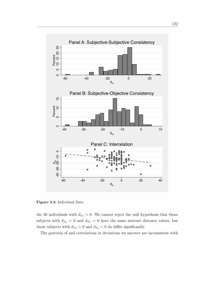
132

05

1015

2025

Perc

ent

-60 -40 -20 0 20dSi

Panel A: Subjective-Subjective Consistency

05

1015

Perc

ent

-40 -30 -20 -10 0 10dMi

Panel B: Subjective-Objective Consistency

-40

-30

-20

-10

0d M

i

-60 -40 -20 0 20 40dSi

Panel C: Interrelation

Figure 3.3: Individual Data

the 20 individuals with dS,i > 0. We cannot reject the null hypothesis that thosesubjects with dS,i < 0 and dS,i = 0 have the same mixture distance values, butthose subjects with dS,i > 0 and dS,i < 0 do differ significantly.

The patterns of and correlations in deviations we uncover are inconsistent with

133

both MEU and KMM preferences. First, MEU predicts zero Subjective-Objectiveinconsistencies which is soundly rejected in the data. Second, KMM under theexponential formulation would predict the same pattern and so is also rejectedin the data. KMM under the power formulation with θ > 0 predicts that ifdS,i < 0, then dM,i > 0, and there should exist a negative correlation between thetwo.43 Though the full data set do provide a negative correlation, the correlationis not robust and the general location of the data (dMi < 0) is not in accord withprediction. An alternative formulation of KMM featuring a concave aggregatorwith increasing absolute concavity may be able to match broad features of thedata, but the lack of correlation between dS,i < 0 and dM,i > 0 potentially suggestsa formulation where these two features are independent.

Additional Inconsistencies: Dominance In addition to Subjective-Subjectiveand Subjective-Objective inconsistencies, the individual data afford the opportu-nity to investigate other potentially interesting patterns. Chief among these aresituations in which one can compare a subjective-objective mixture with a purelyobjective act for which a dominance relation maintains. Indeed, our data havemany such situations and we were surprised to see substantial violations of domi-nance.

We investigate situations in which individuals value the subjective portion of anact, g, higher than it’s best possible outcome, h, or lower than its worst possibleoutcome, l. That is, we investigate whether the following inequalities are violated:

qαl+(1−α)h < qαg+(1−α)h < qαh+(1−α)h.

Each one of these comparisons is indirect in the sense that the valuations comefrom different tasks.

To begin, 10 of 111 subjects (9%) have lower valuations for f and g than for l,valuing an ambiguous draw lower than its worst possible outcome.44 In movingalong the series of mixtures between given acts and h and l subjects have additional

43 That is under the power formulation, the greater is θ, the lower is dS,i and the higher is dM,i.44 Such individuals have disproportionately lower values for dS,i with a mean of -20.5 (s.d.

=16.91) relative to the average of the other 101 subjects of −5.15 (10.43), (t(109) = 4.17, p <0.01). No difference in mixture distances is observed.

134

opportunities to violate dominance either by valuing the subjective portion too low(in the case of h) or valuing it too high (in the case of l). In total, subjects have 6opportunities to violate dominance when mixing with h and 6 opportunities whenmixing with l. Interestingly, different subjects violate dominance in different waysand do so on multiple occasions.

Table 3.4 presents count measures of dominance violations and the relation-ship between dominance violations and δS,i. Dominance violations are frequentthroughout the data, and are substantially more prevalent when considering mix-tures with h as oppposed to l.45 When mixing with the high-paying act h vio-lations are more prevalent among ambiguity averse, δS,i < 0, subjects (p < 0.01,two-sample Kolmogorov-Smirnov test). Indeed, among δS,i < 0 subjects only 16%never violate dominance while this is the case for more than 70% of the non-aversesubjects. For mixtures involving the low-paying act l, in contrast, ambiguity seek-ing subjects δS,i > 0 are more likely to violate dominance (p < 0.01, two-sampleKolmogorov-Smirnov test).46

An initial view of our dominance violations suggests subject errors, potentiallyindicative of subject confusion. Though this is one potential explanation, theextent of correlation with frequently observed experimental findings such as Ells-berg paradox behavior is a sign of regularity. Hence, we are hesitant to drawsuch conclusions. Instead, we recognize the inconsistency of dominance violationswith all considered models, both SEU and non-SEU, and present the violationsas evidence of an incomplete understanding of attitudes towards ambiguity whichperhaps future work can rationalize.

Our dominance violations are observed when comparing subjective to objectivebet evaluations. The majority of violations are in the direction of valuing a sub-jective act below its worst possible objective counterpart. For such observations,beliefs and risk aversion will not be sufficient to rationalize the data.47 As these

45 80% of subjects have zero or one violation of the form where the subjective act is valued higherthan its best possible outcome (mixing with l), while only 55% of subjects have zero or oneviolation of the form where the subjective act is valued lower than its worst possible outcome(mixing with h).

46 There is also a significant correlation between dominance violations when mixing with l anddM,i, (ρ = −0.504, p < 0.01). No significant correlation exists for dominance violations whenmixing with h and dM,i, (ρ = −0.034, p = 0.72).

47 Violating dominance is akin to believing a subjective act as consisting of more than 100%

135

0 1 2 3 4 5 6

Dominance Violationswhen mixing with h

δS,i > 0(N=20) 70.00 15.00 10.00 5.00 0.00 0.00 0.00δS,i = 0 (N=23) 78.26 13.04 8.70 0.00 0.00 0.00 0.00δS,i < 0 (N=68) 16.18 19.12 19.12 23.53 14.71 2.94 4.41Total (N=111) 38.74 17.12 15.32 15.32 9.01 1.80 2.70

Dominance Violationswhen mixing with l

δS,i > 0 (N=20) 10.00 25.00 25.00 20.00 10.00 5.00 5.00δS,i > 0 (N=23) 73.91 13.04 4.35 4.35 0.00 4.35 0.00δS,i < 0 (N=68) 69.12 19.12 11.76 0.00 0.00 0.00 0.00Total (N=111) 59.46 18.92 12.61 4.50 1.80 1.80 0.90

Table 3.4: Number of Individual Dominance Violations

violations are delivered through indirect comparisons, this is potentially suggestiveof explicit costs of consideration for subjective acts. In Appendix 3.A4 we provideestimates specifically accounting for such consideration costs. In our preferredspecification, Table 3.A2, column (4), consideration costs for subjective acts f andg are found to be around 4 percentage points. That is, not considering ambiguity isestimated be worth about a 4% chance of winning $30. We reject the null hypoth-esis of zero consideration costs at all conventional levels, (χ2(2) = 29.2, p < 0.01).

3.5 Discussion and Conclusion

Subjective Expected Utility (SEU) provides a representation of choice that is of-ten rejected by urn paradoxes of the form presented by Ellsberg (1961). Suchphenomena draw attention to inconsistencies between two subjective acts. In re-turning to the consistency implications of SEU, our tests also draw attention toinconsistencies for subjective-objective mixtures. Analyzing subjective-objectiveinconsistencies is critical because non-SEU models are potentially separable alongthis dimension. That is, though the popularized models of Max-min ExpectedUtility (MEU) (Gilboa & Schmeidler, 1989) and Klibanoff et al. (2005) (KMM)both deliver inconsistencies between two subjective bets, only KMM can deliverSubjective-Objective inconsistencies. Under MEU’s relaxed independence axiom,Certainty Independence, one may carry pessimistic beliefs with respect to a givenact, but that pessimism must be consistently applied to all subjective-objective

low-paying marbles.

136

mixtures. Under KMM, mixing with any act yields hedging benefits, includingmixing with objective lotteries.

We document Subjective-Subjective inconsistencies in the form of the Ellsberg(1961) two-color example by comparing the average valuation of two complemen-tary acts, f and g, to the valuation of an objective 50-50 mixture, 1

2h + 1

2l. Sub-

jective acts, on average, are valued around 9% below their objective counterpartand 60% of subjects are inconsistent in the Ellsberg sense. The average behavioris consistent with believing a fully ambiguous jar contains around 70% low-payingmarbles regardless of whether the act in question is f or g.

The novel result of our experiment is the documentation of Subjective-Objectiveinconsistencies. Our results point to a “directed pessimism" wherein subjectiveacts are treated differently depending on whether they are mixed with high or lowoutcomes. Individuals do not treat ambiguous jar portions identically when mixingwith high and low. Rather, the average behavior is consistent with believing theambiguous portion is around 90% low-paying marbles when mixing with the highoutcome, h, and only around 55% low-paying marbles when mixing with the lowoutcome, l. Further, 95% of subjects exhibit such directed pessimism and it islargely independent of standard Ellsberg-style behavior.

The collection of behavior lies outside both MEU and popularized functionalforms for KMM. However, given the flexibility of the KMM model, the broadpatterns could potentially be accommodated by alternative functional forms withspecific restrictions on the nature of the aggregator function, ϕ(·). Hence, ourresults on the collection of Subjective-Subjective and Subjective-Objective incon-sistencies may helpfully distinguish both between competing non-SEU models and,within the class of smooth models, the nature of preferences.

Our individual data allow us to investigate a further pattern of inconsistencyin comparisons between subjective and objective acts. In particular our datashow a prominence of dominance violations, particularly for mixtures with thehigh outcome, h. That is, an ambiguous jar portion is treated as potentiallybeing worse than its worst possible distribution. Such behavior lies outside of allconsidered SEU and non-SEU models. Though one might view such behavior asmistaken, it does correlate highly with standard Ellsberg-style behavior. Hence,we are hesitant to jump to conclusions. We present the violations as primarily

137

suggestive, potentially indicating some costs of consideration for ambiguous acts.Importantly, such consideration costs need not be large to generate our effects.Estimates of such cost parameters are around a 4% chance of winning $30. Thatis, subjects are willing to give up around $1.20 in expected value to not have tothink about ambiguity.

Given our results lie outside both SEU and current non-SEU models of choice,they present an important challenge for theoretical developments of decision-making under ambiguity. Articulating such a model is outside of the scope ofthis work, but our analysis points to several key elements. Mixture dependentambiguity attitudes could be a feature of such a model, deliverable either throughnon-linearities as in KMM, or through explicit statement of directed pessimism.Consideration costs could be another feature, deliverable either through changingcurvature under ambiguity or fixed costs. In Appendix 3.A4, we estimate a bench-mark of SEU and then allow explicitly for non additive beliefs of the MEU form,mixture dependence in beliefs, and fixed consideration costs. Though far from anarticulated model of choice and without even a hint of the necessary axiomaticfoundation, this suggestive first step matches well the key components of the data.

Even without a model, we believe insights can be drawn for applied work relyingon reduced form results. In particular, the intuition of directed pessimism mayshed light on a variety of phenomena in risk taking. One natural application mightbe the environment of rainfall index insurance in developing countries. Take up ofsuch products has been generally low (for discussion, see e.g., Chantarat, Mude,Barrett, & Carter, 2013). The value of index insurance can be viewed as the valu-ation of a subjective act and standard economics holds that low demand is drivenby beliefs that make the product unattractive. Now consider offering the contractwhere half the time the person receives the index insurance payout and half thetime they receive a high outcome regardless of the realized event. Under the viewof directed pessimism, this would make individuals substantially more pessimisticfor the ambiguous portion of the act and so make insurance take-up more likely.Though such a product has, to our knowledge, never been tested, it is in some waysclose in spirit to a financial innovation occurring in the life insurance industry inthe 19th century. Tontine life insurance was introduced at a moment of stagnationin the term life insurance industry (Ransom & Sutch, 1987). The product took

138

the insurance premiums paid by policy holders and, instead of paying out annualdividends, invested the surplus premiums in a tontine account. At the end of theterm, the tontine account was paid to survivors current on their policies. Demandincreased dramatically such that by 1906, before tontine insurance became illegal,an estimated two-thirds of policies were of the form (Ransom & Sutch, 1987).In effect, the innovation made the bad state worse (as no premium surplus divi-dends were received) and the good state better (as one won the survivor lottery).With objective probabilities, no dependence on others, and actuarially fair valuesthis should, in the presence of risk aversion, lead to less demand. Stylistically,the tontine policy would generate a mean preserving spread of the initial policy.Additionally, however, the tontine mixed the insurance act in question with anadditional act based upon others’ deaths and policy maintenance. For the healthyand organized this may be mixing with quite a good act, with directed pessimismleading to increased demand, and, interestingly, positive selection. Though theseare only two examples, we believe the insights from this experiment for directedpessimism, as well as those for consideration costs, may prove helpful in otherapplied settings.

139

3.6 References

Abdellaoui, M., Baillon, A., Placido, L. L., & Wakker, P. P. (2010). The rich do-main of uncertainty: source functions and their experimental implementation.The American Economic Review, 101 (April), 695–723.

Abdellaoui, M., Klibanoff, P., & Placido, L. (2011). Ambiguity and compound riskattitudes :

Allais, M. (1953). Le comportement de l’homme rationnel devant le risque: critiquedes postulats et axiomes de l’ecole americaine. Econometrica, 21 (4), 503–546.

Anscombe, F. & Aumann, R. (1963). A definition of subjective probability. TheAnnals of Mathematical Statistics, 34 (1), 199–205.

Azriely, Y., Chambers, C. P., & Healy, P. J. (2014). Incentives in experiments: atheoretical analysis.

Bade, S. (2014). Randomization devices and the elicitation of ambiguity aversepreferences.

Baillon, A., Halevy, Y., & Li, C. (2014). Experimental elicitation of ambiguityattitude.

Baillon, A. & Bleichrodt, H. (2011). Testing ambiguity models through the mea-surement of probabilities for gains and losses.

Becker, S. W. & Brownson, F. O. (1964). What price ambiguity? or the role ofambiguity in decision-making. The Journal of Political Economy, 72 (1), 62–73.

Binmore, K., Stewart, L., & Alex Voorhoeve. (2013). How much ambiguity aver-sion? - finding indifferences between ellsberg’s risky and ambiguous bets.

Bleichrodt, H., Abellan-Perinan, J. M., Pinto-Prades, J. L., & Mendez-Martinez,I. (2007). Resolving inconsistencies in utility measurment under risk: tests ofgeneralizations of expected utility. Management Science, 53 (3).

Camerer, C. & Weber, M. (1992). Recent developments in modeling preferences:uncertainty and ambiguity. Journal of Risk and Uncertainty, 5 (4), 325–370.

Chantarat, S., Mude, A. G., Barrett, C. B., & Carter, M. R. (2013). Designingindex-based livestock insurance for managing asset risk in northern kenya.Journal of Risk and Insurance, 80 (1), 205–237.

140

Charness, G., Karni, E., & Levin, D. (2012). Ambiguity attitudes : an experimentalinvestigation.

Curley, S. P. & Yates, J. F. (1985). The center and range of the probability inter-val as factors affecting ambiguity preferences. Organizational Behavior andHuman Decision Processes, 36, 273–287.

Ellsberg, D. (1961). Risk, ambiguity, and the savage axioms. The Quarterly Journalof Economics, 75 (4), 643.

Epstein, L. & Schneider, M. (2010). Ambiguity and asset markets. NBER WorkingPaper, (16181).

Farquhar, P. H. (1984). Utility assessment methods. Management Science, 30 (11),1283–1300.

Ghirardato, P., Maccheroni, F., & Marinacci, M. (2004). Differentiating ambiguityand ambiguity attitude. Journal of Economic Theory, 118 (2), 133–173.

Gilboa, I. & Marinacci, M. (2011). Ambiguity and the bayesian paradigm.Gilboa, I. & Schmeidler, D. (1989). Maxmin expected utility with non-unique prior.

Journal of Mathematical Economics, 18, 141–153.Halevy, Y. (2007). Ellsberg revisited: an experimental study. Econometrica, 75 (2),

503–536.Hardy, G. H., Littlewood, J. E., & Pólya, G. (1934). Inequalities (1991st ed.).

Cambridge Mathematical Library. Cambridge, UK: Cambridge UniversityPress.

Holt, C. (1986). Preference reversals and the independence axiom. The AmericanEconomic Review, 76 (1), 508–515.

Holt, C. A. & Laury, S. K. (2002). Risk aversion and incentive effects. The Amer-ican Economic Review, 92 (5), 1644–1655.

Hong, C. S., Bin, M., & Songfa, Z. (2013). Partial ambiguity.Karni, E. & Safra, Z. (1987). "Preference reversal"and the observability of prefer-

ences by experimental methods. Econometrica, 55 (3), 675–685.Klibanoff, P., Marinacci, M., & Mukerji, S. (2005). A smooth model of decision

making under ambiguity. Econometrica, 73 (6), 1849–1892.Magat, W. A., Viscusi, W. K., & Huber, J. (1996). A reference lottery metric for

valuing health. Management Science, 42 (8), 1118–1130.

141

McCord, M. & de Neufville, R. (1986). ‘lottery equivalents’: reduction of the cer-tainty effect problem in utility assignment. Management Science, 32 (1), 56–60.

Meier, S. & Sprenger, C. (2010). Present-biased preferences and credit card bor-rowing. American Economic Journal - Applied Economics, 2 (1), 193–210.

Oliver, A. (2005). Testing the internal consistency of the lottery equivalents methodusing health outcomes. Health Economics, 14, 149–159.

Oliver, A. (2007). A qualitative analysis of the lottery equivalents method. Eco-nomics and Philosophy, 23, 185–204.

Pratt, J. (1964). Risk aversion in the small and in the large. Econometrica, 32 (1-2),122–136.

Raiffa, H. (1961). Risk, ambiguity, and the savage axioms: comment. The QuarterlyJournal of Economics, 75 (4), 690–694.

Ransom, R. L. & Sutch, R. (1987). Tontine insurance and the armstrong inves-tigation: a case of stifled innovation 1868–1905. The Journal of EconomicHistory, 47 (2), 379–390.

Samuelson, P. A. (1953). Utilité, préfèrence et probabilité. In Colloques inter-nationaux du centre natlonal de la recherche scientifique (econometrie) 40(pp. 141–150).

Savage, L. J. (1953). Une axiomatisation de comportement raisonnable face àl’incertitude. In Colloques internationaux du centre natlonal de la recherchescientifique (econometrie) 40 (pp. 29–33).

Savage, L. J. (1954). The foundations of statistics. New York: John Wiley andSons.

Schmeidler, D. (1989). Probability and expected utility without additivity. Econo-metrica, 57 (3), 571–587.

Stewart, M. B. (1983). On least squares estimation when the dependent variableis grouped. The Review of Economic Studies, 50 (4), 737–753.

Varian, H. R. (1992). Microeconomic analysis (3rd). New York: Norton.

142

3.7 Appendices

3.A1 KMM Preferences and δM(α, f) / δM(α, g)

In this appendix section we demonstrate that for KMM preferences,

UKMM(f) =

∫S

p(s) ϕ (u(a(s))) ds,

with ϕ(·) strictly increasing and strictly concave everywhere, δM(α, f) ≥ 0 for allα.

We introduce an Ellsberg style jar composed of N red and green marbles. Thestate of the world is determined by the composition of the jar.48 Hence the statespace has N+1 elements and we can label states S = {0, .., N} by how many of themarbles in the jar are red. We establish the set of consequences as X = {0, x, y}with 0 < x < y. Under the state space as defined above our four basic acts are:

• f : in each state i: yields y with probability iN

, yields x with probability N−iN

.• g: in each state i: yields y with probability N−i

N, yields x with probability

iN

.• h: in each state i: yields y with probability 1.• l: in each state i: yields x with probability 1.

Consider the act f , which yields the KMM utility

UKMM(f) =N∑i=0

πiϕ

(i

Nu(y) +

N − i

Nu(x)

)

where πi is the subjective probability the decision maker attaches to the statewhere i marbles are red yielding y and N− i marbles are green yielding x. Rewritethis as

UKMM(f) =N∑i=0

πiϕ(Ai),

48 We use this state space rather than one in which the state is determined by the color of thedrawn marble because while the two state space formulations are equivalent under SEU, MEUand CEU (the probabilities in the compositions-as-states formulation can be reduced to yieldthe draws-as-states formulation) assuming the binary state space is not without loss underKMM

143

where Ai =iNu(y) + N−i

Nu(x). Now consider the mixture acts αf + (1− α)h and

αf + (1− α)l with α ∈ (0, 1),

UKMM(αf + (1− α)h) =N∑i=0

πiϕ(αAi + (1− α)u(y)),

UKMM(αf + (1− α)l) =N∑i=0

πiϕ(αAi + (1− α)u(x)).

Note, by the strict concavity of ϕ(·)

ϕ(αAi + (1− α)u(y)) > αϕ(Ai) + (1− α)ϕ(u(y))

ϕ(αAi + (1− α)u(x)) > αϕ(Ai) + (1− α)ϕ(u(x))

Let ϵyAi> 0 and ϵxAi

> 0 be defined such that

ϕ(αAi + (1− α)u(y)) = αϕ(Ai) + (1− α)ϕ(u(y)) + ϵyAi

ϕ(αAi + (1− α)u(x)) = αϕ(Ai) + (1− α)ϕ(u(x)) + ϵxAi

Hence UKMM(αf + (1− α)h)− UKMM(αf + (1− α)l) is

N∑i=0

πi{[αϕ(Ai) + (1− α)ϕ(u(y)) + ϵyAi]− [αϕ(Ai) + (1− α)ϕ(u(x)) + ϵxAi

]},

or

(1− α)ϕ(u(y))− (1− α)ϕ(u(x)) +N∑i=0

πi[ϵyAi− ϵxAi

].

Now consider the mixture act αh+ (1− α)l with corresponding KMM utility

UKMM(αh+ (1− α)l) = ϕ(αu(y) + (1− α)u(x)),

Note, by the strict concavity of ϕ(·)

ϕ(αy + (1− α)u(x)) > αϕ(u(y)) + (1− α)ϕ(u(x))

144

Let ϵ be defined such that

ϕ(αy + (1− α)u(x)) = αϕ(u(y)) + (1− α)ϕ(u(x)) + ϵ.

Hence,UKMM(αh+ (1− α)l) = αϕ(u(y)) + (1− α)ϕ(u(x)) + ϵ.

Now consider UKMM(αf+(1−α)h)−UKMM(αf+(1−α)l)+UKMM(αh+(1−α)l).Under SEU such a sum is equal to the utility of the highest outcome, y, or, bynormalization equal to 1. Under KMM this sum is

(1−α)ϕ(u(y))− (1−α)ϕ(u(x)) +αϕ(y) + (1−α)ϕ(u(x)) + ϵ+N∑i=0

πi[ϵyAi− ϵxAi

],

or

ϕ(u(y)) +N∑i=0

πi[ϵyAi− ϵxAi

+ ϵ],

Normalizing ϕ(u(y)) = 1 this yields

1 +N∑i=0

πi[ϵyAi− ϵxAi

+ ϵ],

We now recall the definition of δM(α, f) as

δM(α, f) = U(αf + (1− α)h)− U(αf + (1− α)l) + U(αh+ (1− α)l)− 1.

Subtracting 1 from the above we obtain only the sum of error terms,

N∑i=0

πi[ϵyAi− ϵxAi

+ ϵ].

We can now investigate the sign of ϵyAi−ϵxAi

+ϵ to recover whether δM(α, f) ≥ 0

or δM(α, f) ≤ 0. We wish to prove that if ϕ(·) is concave, ϵyAi− ϵxAi

+ ϵ ≥ 0 forevery Ai and for every α such that δM(α, f) ≥ 0 for every α.

Note that for a given u(x) < Ai < u(y), the error terms are each associated withthe distance from a chord between two points and the functions ϕ(·). The location

145

●

●

●

●

●

●

u(x) u(y)Ai

ε

εyAi

εxAi

Figure 3.A1: A Standard Case

on the chord is determined by the mixture α. Figure 3.A1 illustrates a standardcase with ϵyAi

and ϵ in red and ϵxAiin blue. We can investigate the limiting

case that maximizes ϵxAiand minimizes ϵyAi

and ϵ. This is done by replacing thefunction away from u(x) with the extended chord between Ai and u(y). This isillustrated in Figure 3.A2.

In the limiting case, ϵyAi= 0. Hence, the relevant comparison is between ϵxAi

and ϵ. Note that the slope of the extended chord in Figure 3.A2 is

ϕ(u(y))− ϕ(Ai)

u(y)− Ai

.

146

●●

●

●

●

●

u(x) u(y)Ai

ε

εyAi

εxAi

Figure 3.A2: Limiting Case

Now consider the slope between the points, (αAi + (1 − α)u(x), αϕ(Ai) + (1 −α)ϕ(u(x))) and ((αu(y) + (1− α)u(x), αϕ(u(y) + (1− α)ϕ(u(x))). This slope is

[αϕ(u(y) + (1− α)ϕ(u(x))]− [αϕ(Ai) + (1− α)ϕ(u(x))]

[αu(y) + (1− α)u(x)]− [αAi + (1− α)u(x)]=

ϕ(u(y))− ϕ(Ai)

u(y)− Ai

,

parallel to the extended chord. Hence, a parallelogram is constructed with theerror terms, ϵ and ϵxAi

and the chords connecting their endpoints. Because in aparallelogram opposite sides are of equal length, in the limiting case ϵ = ϵxAi.

As ϕ(·) is assumed strictly concave everywhere, the limiting case occurs only ifi = 0 or i = N . In all other cases ϵ is strictly bounded below by its limiting value

147

and ϵxAi is strictly bounded above by its limiting value. Hence, ϵ ≥ ϵxAi alwaysand ϵyAi − ϵxAi + ϵ ≥ 0. The same graphical technique can be applied for every Ai

and for every α. Hence, for a strictly concave and increasing ϕ(·) we conclude thatϵyAi

− ϵxAi+ ϵ ≥ 0 for every Ai and for every α. Moreover, for all 0 < i < N the

inequality is strict. For strictly concave and strictly increasing ϕ(·), δM(α, f) ≥ 0

for every α. One can easily prove the opposite for a strictly convex and strictlyincreasing ϕ(·).

148

3.A2 KMM Preferences and dM(α, f) / dM(α, g)

In this appendix section we prove results about the shape of the uncertainty equiv-alent functions and the empirical mixture differences dM(α, f) and dM(α, g) underKMM. The setting is identical to the setting assumed in the previous section.

Theorem 1. For a KMM agent with strictly increasing and four times continu-ously differentiable utility aggregator ϕ (·) uncertainty equivalents for the subjective-objective mixtures αf + (1− α)(pl + (1− p)h) with α ∈ (0, 1) and p ∈ [0, 1] are

• a concave function of the mixture probability α if ϕ′′(·) < 0 and the coefficientof absolute ambiguity tolerance −ϕ′(·)

ϕ′′(·) is convex, and• a convex function of the mixture probability α if ϕ′′(·) > 0 and the coefficient

of absolute ambiguity tolerance −ϕ′(·)ϕ′′(·) is concave.

Proof. The proof is adapted from the proof of Theorem 106 in Hardy, Littlewood,and Pólya (1934). The uncertainty equivalent q for the subjective-objective mix-ture αf + (1− α)(pl + (1− p)h) satisfies the following equality:

ϕ (qu(y) + (1− q)u (0)) =N∑i=0

πiϕ

(α

(i

Nu(y) +

(1− i

N

)u(x)

)

+ (1− α) ((1− p)u(y) + pu(x))

)

Since ϕ(·) is strictly increasing, it is invertible. Therefore we can write q explicitlyas

q =ϕ−1

(∑Ni=0 πiϕ

(α(

iNu(y) +

(1− i

N

)u(x)

)+ (1− α) ((1− p)u(y) + pu(x))

))− u(0)

u(y)− u (0)

In the following define pi ≡ iN+p−1 and Ei ≡ u(x)+(αpi + (1− p)) (u(y)− u(x)).

149

The last expression can then be written more concisely as

q =ϕ−1

(∑Ni=0 πiϕ (Ei)

)− u(0)

u(y)− u (0)

Taking partial derivatives w.r.t α twice:

∂q

∂α=u(y)− u(x)

u(y)− u (0)×(ϕ−1)′ ( N∑

i=0

πiϕ (Ei)

)[N∑i=0

πiϕ′(Ei) pi

]∂2q

∂α2=(u(y)− u(x))2

u(y)− u (0)

×[ (

ϕ−1)′′ ( N∑

i=0

πiϕ (Ei)

)[N∑i=0

πiϕ′(Ei) pi

]2

+(ϕ−1)′ ( N∑

i=0

πiϕ (Ei)

)[N∑i=0

πiϕ′′(Ei) p

2i

]]

=(u(y)− u(x))2

u(y)− u (0)×[ −ϕ

′′(ϕ−1

(∑Ni=0 πiϕ (Ei)

))[ϕ′(ϕ−1

(∑Ni=0 πiϕ (Ei)

))]3[

N∑i=0

πiϕ′(Ei) pi

]2

+1

ϕ′(ϕ−1

(∑Ni=0 πiϕ (Ei)

)) [ N∑i=0

πiϕ′′(Ei) p

2i

] ]

A necessary and sufficient condition for global concavity of q is that the secondderivative is non-positive throughout, i.e. that[

ϕ′

(ϕ−1

(N∑i=0

πiϕ (Ei)

))]2 [ N∑i=0

πiϕ′′(Ei) p

2i

]

− ϕ′′

(ϕ−1

(N∑i=0

πiϕ (Ei)

))[N∑i=0

πiϕ′(Ei) pi

]2≤ 0

150

or equivalently that[ϕ

′(ϕ−1

(∑Ni=0 πiϕ (Ei)

))]2ϕ′′(ϕ−1

(∑Ni=0 πiϕ (Ei)

)) ≤

[∑Ni=0 πiϕ

′(Ei) pi

]2∑N

i=0 πiϕ′′ (Ei) p2i

The numerator of the right-hand side expression can be bounded above by theCauchy-Schwartz inequality:

[N∑i=0

πiϕ′(Ei) pi

]2=

⎡⎣ N∑i=0

√ϕ′′ (Ei) πipi

√πi (ϕ

′ (Ei))2

ϕ′′ (Ei)

⎤⎦2

≤

[N∑i=0

ϕ′′(Ei) πip

2i

]·

[N∑i=0

πi

(ϕ

′(Ei)

)2ϕ′′ (Ei)

]

Dividing this inequality by the denominator of the original expression yields alower bound:

[ϕ

′(ϕ−1

(∑Ni=0 πiϕ (Ei)

))]2ϕ′′(ϕ−1

(∑Ni=0 πiϕ (Ei)

)) ≤

[∑Ni=0 ϕ

′′(Ei) πip

2i

]·

[∑Ni=0 πi

(ϕ′(Ei)

)2

ϕ′′ (Ei)

]∑N

i=0 πiϕ′′ (Ei) p2i

≤

[∑Ni=0 πiϕ

′(Ei) pi

]2∑N

i=0 πiϕ′′ (Ei) p2i

The first inequality is therefore a sufficient condition for the second. After can-celling common terms we are left with[

ϕ′(ϕ−1

(∑Ni=0 πiϕ (Ei)

))]2ϕ′′(ϕ−1

(∑Ni=0 πiϕ (Ei)

)) ≤N∑i=0

πi

(ϕ

′(Ei)

)2ϕ′′ (Ei)

Define Ki = ϕ(Ei) and

Φ(Ki) =(ϕ′(ϕ−1(Ki)))

2

ϕ′′(ϕ−1(Ki))

151

and rewrite the above as

Φ(∑

πiKi) ≤∑

πiΦ(Ki)

The convexity of Φ(·) is therefore sufficient for the concavity of the uncertaintyequivalents.

The first two derivatives of Φ(·) are

Φ′(K) =2ϕ′(E)ϕ′′(E) dE

dKϕ′′(E)− (ϕ′(E))2ϕ′′′(E) dE

dK

(ϕ′′(E))2

=d

dE

(ϕ′(E)

ϕ′′(E)

)ϕ′(E)

dE

dK+

ϕ′(E)(ϕ′′(E))2

ϕ′′(E))2dE

dK

=d

dE

(ϕ′(E)

ϕ′′(E)

)+ 1

Φ′′(K) =1

ϕ′(E)

d2

dE2

(ϕ′(E)

ϕ′′(E)

)

Φ(·) is convex if its second derivative is positive, i.e. if ϕ′(E)ϕ′′(E)

is convex, which

is equivalent to the coefficient of absolute risk tolerance −ϕ′(E)ϕ′′(E)

being concave.The proof for the case when ϕ′′(·) > 0 and the coefficient of absolute ambiguitytolerance −ϕ′(·)

ϕ′′(·) is convex is analogous and therefore omitted.

How restrictive is the condition that the coefficient of absolute ambiguity tol-erance −ϕ′(·)

ϕ′′(·) be concave? Not very restrictive at all. In fact the whole class ofHAAA (hyperbolic absolute ambiguity aversion) functions of the form

ϕ(x) =1− γ

γ

(αx

1− γ+ β

)γ

has coefficients of absolute ambiguity tolerance that are linear and therefore bothconvex and concave. The function above nests the popular exponential ϕ(x) =

−e−θx and power ϕ(x) = x1−θ

1−θfunctions.

We next prove a result about the sign of the empirical mixture differencesδM(α, f) and δM(α, g), which is our main object of interest. This sign will dependupon the difference between the sign of the difference between the uncertaintyequivalents of the two mixtures, which will in turn depend upon whether uncer-

152

tainty equivalents as a function of α are more or less concave when mixing withh or mixing with l (for an illustration, see Figure 3.A3). Intuitively mixing withany constant act has three effects in KMM:

1. It pulls the distribution of state expected utilities in the direction of theexpected utility of the constant act. This is the only effect that plays a rolein SEU.

2. It reduces the spread of state expected utilities. As shown in the previoustheorem, under fairly general assumptions ambiguity averse KMM agents, incontrast to SEU agents, value this reduction because state expected utilitiesare aggregated with the concave function ϕ(·). This increase in utility isreflected in an additional increase in uncertainty equivalents.

3. There may be an additional effect on the uncertainty equivalents that de-pends on the exact functional form of ϕ(·) in a way that is analogous to thebehavior of risk premia in expected utility under risk. Just as risk premiadepend on the Arrow-Pratt coefficient of absolute risk aversion (See Pratt,1964, , Theorem 2) uncertainty equivalents depend on the coefficient of ab-

α

q

1

0.25 0.5 0.75 1u(x)−u(0)u(y)−u(0)

CI

KMM

Figure 3.A3: Uncertainty equivalents q under Certainty Independence (CI) and KMMwith decreasing absolute ambiguity aversion. Mixtures displayed are those with the actsh and l

153

solute ambiguity aversion. If the coefficient of absolute ambiguity aversionϕ′′(u)ϕ′(u)

is decreasing in u, for example, this means mixing with h pulls thedistribution of state expected utilities into a region in which ϕ(·) is less con-cave, which raises the uncertainty equivalent further. Conversely, in this casemixing with l pulls the distribution of state expected utilities into a regionin which ϕ(·) is more concave, which lowers the uncertainty equivalent.

Theorem 2. Assume a KMM agent with strictly increasing and twice continuouslydifferentiable utility aggregator ϕ (·).

• dm(α, f) > 0 and dm(α, g) > 0 for all α if the coefficient of absolutel ambi-guity aversion −ϕ′′(u)

ϕ′(u)is strictly decreasing in u

• dm(α, f) = 0 and dm(α, g) = 0 for all α if the coefficient of absolutel ambi-guity aversion −ϕ′′(u)

ϕ′(u)is constant

• dm(α, f) < 0 and dm(α, g) < 0 for all α if the coefficient of absolutel ambi-guity aversion −ϕ′′(u)

ϕ′(u)is strictly increasing in u

Proof. By definition the mixture difference dm(α, f) is given by the following linearcombination of uncertainty equivalents:

dm(α, f) = qαf+(1−α)h − qαf+(1−α)l + qαh+(1−α)l − 1

Under KMM uncertainty equivalents of the mixtures αf+(1−α)c where c ∈ {l, h}denotes the two objective/constant acts can be written as

qαf+(1−α)a =ϕ−1

(∑Ni=0 πiϕ (αU(f(i)) + (1− α)U(c))

)− u(0)

u(y)− u(0)

where U(c) = u(x) for act l and U(c) = u(y) for act h are the von-Neumann-Morgenstern utilities of the objective acts and U(f(i)) = i

Nu(y) +

(1− i

N

)u(x) is

the vNM-utility of the lottery that f yields in state i. The uncertainty equivalentof αh+ (1− α)l is simply

qαh+(1−α)l =αu(y) + (1− α)u(x)− u(0)

u(y)− u(0)

154

Substituting in these uncertainty equivalents yields

dm(α, f) =ϕ−1

(∑Ni=0 πiϕ (αU(f(i)) + (1− α)u(y))

)− u(0)

u(y)− u(0)

−ϕ−1

(∑Ni=0 πiϕ (αU(f(i)) + (1− α)u(x))

)− u(0)

u(y)− u(0)

+αu(y) + (1− α)u(x)− u(0)

u(y)− u(0)− 1

or, after some rearrangement

dm(α, f) =1

u(y)− u(0)×[

ϕ−1

(N∑i=0

πiϕ (αU(f(i)) + (1− α)u(y))

)

− αϕ−1

(N∑i=0

πiϕ (U(f(i)))

)− (1− α)u(y)

− ϕ−1

(N∑i=0

πiϕ (αU(f(i)) + (1− α)u(x))

)

+ αϕ−1

(N∑i=0

πiϕ (U(f(i)))

)+ (1− α)u(x)

]

Define ∆(U(c)) as

∆(U(c)) =ϕ−1

(N∑i=0

πiϕ (αU(f(i)) + (1− α)U(c))

)

− αϕ−1

(N∑i=0

πiϕ (U(f(i)))

)− (1− α)U(c)

155

and take the partial derivative with respect to U(c):

∂∆(U(c))

∂U(c)= (1− α)

[ (ϕ−1)′( N∑

i=0

πiϕ (αU(f(i)) + (1− α)U(c))

)(

N∑i=0

πiϕ′ (αU(f(i)) + (1− α)U(c))

)− 1

]

= (1− α)

⎡⎣ ∑Ni=0 πiϕ

′ (αU(f(i)) + (1− α)U(c))

ϕ′(ϕ−1

(∑Ni=0 πiϕ (αU(f(i)) + (1− α)U(c))

)) − 1

⎤⎦∂∆(U(c))∂U(c)

> 0 if

N∑i=0

πiϕ′ (αU(f(i)) + (1− α)U(c)) > ϕ′

(ϕ−1

(N∑i=0

πiϕ (αU(f(i)) + (1− α)U(c))

))

that is, if the average marginal utility of a mixture is larger than the marginalutility at the certainty equivalent of that mixture. To see that this is true if −ϕ′′(·)

ϕ′(·)

is decreasing, consider the indifference condition for the certainty equivalent:

N∑i=0

πiϕ (αU(f(i)) + (1− α)U(c)) = ϕ

(ϕ−1

(N∑i=0

πiϕ (αU(f(i)) + (1− α)U(c))

))

Now modify both the mixture and its certainty equivalent by adding an ε > 0

to the vNM utility (not to the prize) in every state. Because the function hasdecreasing absolute ambiguity aversion adding this additional utility means shewill now prefer the modified mixture over the modified certainty equivalent49:

N∑i=0

πiϕ (αU(f(i)) + (1− α)U(c) + ε) > ϕ

(ϕ−1

(N∑i=0

πiϕ (αU(f(i)) + (1− α)U(c))

)+ ε

)

49 The proof of this claim is analogous to the proof that risk premia in choice under risk aredecreasing functions of wealth if the coefficient of absolute risk aversion is decreasing (seePratt, 1964), which implies that such a DARA agent will prefer a risky gamble to its certaintyequivalent after all prizes in the gamble and the certainty equivalent are increased by a smallamount

156

But this must mean that

N∑i=0

πiϕ′ (αU(f(i)) + (1− α)U(c)) > ϕ′

(ϕ−1

(N∑i=0

πiϕ (αU(f(i)) + (1− α)U(c))

))

as desired.

The cases for −ϕ′′(·)ϕ′(·) constant and −ϕ′′(·)

ϕ′(·) increasing are analoguous.

Note that the above result is independent of the sign of ϕ′′(·), i.e. of whetherthe agent is ambiguity averse or ambiguity seeking.

157

3.A3 Full Regression Results

Task Act Midpoints Interval Regression

mean s.e. All AmbiguitySeekingdS,i > 0

AmbiguityNeutraldS,i = 0

AmbiguityAversedS,i < 0

1 14g + 3

4h 83.90 (1.17) 83.90 (1.17) 87.00 (1.54) 88.37 (2.22) 81.47 (1.62)

2 14g + 3

4l 66.91 (1.62) 66.91 (1.61) 68.00 (2.93) 73.80 (3.87) 64.26 (2.02)

3 12g + 1

2h 76.46 (1.21) 76.46 (1.21) 78.00 (1.97) 83.59 (2.62) 73.60 (1.55)

4 12g + 1

2l 68.40 (1.62) 68.40 (1.61) 71.50 (2.85) 75.54 (3.58) 65.07 (2.07)

5 12g + 1

2(12h+ 1

2l) 73.72 (1.40) 73.72 (1.40) 76.50 (2.37) 79.46 (3.08) 70.96 (1.82)

6 34g + 1

4l 68.85 (1.76) 68.85 (1.76) 73.50 (2.79) 77.50 (3.35) 64.56 (2.35)

7 34g + 1

4h 74.12 (1.44) 74.12 (1.44) 78.00 (2.30) 82.93 (2.31) 70.00 (1.93)

8 g 69.80 (1.61) 69.80 (1.60) 76.00 (2.46) 78.80 (3.06) 64.93 (2.08)

9 14l + 3

4h 84.71 (0.84) 84.71 (0.84) 79.00 (2.30) 87.28 (1.70) 85.51 (0.95)

10 12l + 1

2h 76.37 (1.20) 76.37 (1.20) 69.25 (2.39) 78.80 (2.90) 77.65 (1.45)

11 34l + 1

4h 68.76 (1.46) 68.76 (1.45) 66.25 (2.61) 73.80 (3.73) 67.79 (1.80)

12 l 62.41 (1.77) 62.41 (1.76) 60.00 (3.34) 70.76 (4.49) 60.29 (2.13)

13 14f + 3

4h 84.39 (0.78) 84.39 (0.78) 84.50 (1.52) 89.02 (1.81) 82.79 (0.94)

14 14f + 3

4l 66.15 (1.66) 66.15 (1.66) 69.00 (2.82) 72.28 (4.02) 63.24 (2.10)

15 12f + 1

2h 77.09 (1.19) 77.09 (1.19) 80.25 (2.02) 83.59 (2.33) 73.97 (1.54)

16 12f + 1

2l 67.36 (1.73) 67.36 (1.72) 72.00 (2.79) 75.33 (3.65) 63.31 (2.24)

17 12f + 1

2(12h+ 1

2l) 73.09 (1.35) 73.09 (1.34) 76.00 (2.44) 79.46 (2.94) 70.07 (1.71)

18 34f + 1

4l 68.63 (1.69) 68.63 (1.68) 72.25 (3.13) 77.72 (3.28) 64.49 (2.17)

19 34f + 1

4h 73.09 (1.50) 73.09 (1.49) 77.25 (3.40) 81.20 (2.73) 69.12 (1.86)

20 f 69.89 (1.71) 69.89 (1.70) 77.50 (2.16) 78.80 (2.97) 64.63 (2.28)

dS -6.53 (1.14) -6.53 (1.13) 7.50 (1.48) -12.87 (1.24)

H0 : dS = 0 F = 33.10 χ2(1) = 33.39 χ2(1) = 25.85 χ2(1) = 107.00(p < 0.01) (p < 0.01) (p < 0.01) (p < 0.01)

dM(g, 14) -14.26 (1.37) -14.26 (1.36) -14.75 (2.34) -11.63 (2.22) -15.00 (1.97)

dM(g, 12) -15.56 (1.16) -15.56 (1.16) -24.25 (2.28) -13.15 (2.19) -13.82 (1.47)

dM(g, 34) -10.02 (1.06) -10.02 (1.06) -16.50 (2.70) -7.283 (1.87) -9.044 (1.31)

dM(f, 14) -13.00 (1.11) -13.00 (1.10) -18.25 (2.69) -9.457 (2.65) -12.65 (1.27)

dM(f, 12) -13.90 (1.27) -13.90 (1.26) -22.50 (2.97) -12.93 (2.25) -11.69 (1.59)

dM(f, 14) -10.83 (1.17) -10.83 (1.17) -16.00 (3.28) -9.239 (1.74) -9.853 (1.49)

H0 : dM(f, α) = dM(g, α) = 0; χ2(6) = 261.50 χ2(6) = 184.94 χ2(6) = 45.82 χ2(6) = 155.89α ∈ {1

4, 12, 34} (p < 0.01) (p < 0.01) (p < 0.01) (p < 0.01)

H0 : dM(f, α), dM(g, α) χ2(6) = 22.30identical for dS,i > 0 and dS,i < 0 (p < 0.01)

H0 : dM(f, α), dM(g, α) χ2(6) = 4.34identical for dS,i = 0 and dS,i < 0 (p = 0.63)

# Individuals 111 111 20 23 68

Interval regression. Standard errors clustered on individual level. Subjective premium and mixture distances calculated as linearcombinations of regression coefficients. Hypothesis tests across dS,i groups from regression of response on indicators for tasknumber interacted with dS,i group.

Table 3.A1: Mean uncertainty equivalents, subjective premia and mixture distances.

158

3.A4 Estimating Decisionmaking Parameters

Our data are clearly at odds with SEU as well as popular non-SEU formulationssuch as MEU and KMM. Our findings of Subjective-Subjective and Subjective-Objective inconsistency suggest two key features of decision-making: non-uniquebeliefs across subjective acts and a sensitivity of either the perception of ambiguityor subjects’ attitude towards it to mixing subjective acts with either high or lowoutcomes. In this appendix we attempt to explicitly model these two features andprovide corresponding parameter estimates. We additionally provide estimatesrelated to consideration costs for ambiguous acts that may account for the observedviolations of dominance. In the spirit of full disclosure, providing simple parametricmethods for the estimation of beliefs and risk aversion in SEU and non-SEU modelswas an original objective in experimental design. Given the non-adherence of thedata to all considered models of decision making under ambiguity, this exercisemoved from being at the fore to an exploration outside of the theory.

For a given individual who makes j = 1, 2, . . . , J decisions, let p̃green(f) be thebeliefs on the probability of a green marble induced by subjective act f , where agreen marble yields x and a red marble yields y > x. Consider binary objectiveacts, cj, with the same consequences as f , summarized by pcj and mixtures αj ∈[0, 1] representing the degree of ambiguity. Let preferences satisfy SEU such thatthe utility of the mixture αjf + (1− αj)cj is represented as

αj · [p̃green(f)u(x) + (1− p̃green(f))u(y)] + (1− αj) · [pcju(x) + (1− pcj)u(y)].

We consider the equivalent constant act qj over y and 0, summarized by qj suchthat the indifference condition

αj·[p̃green(f)u(x)+(1−p̃green(f))u(y)]+(1−αj)·[pcju(x)+(1−pcj)u(y)] = qju(y)+(1−qj)u(0)

is met. Rearranging terms one arrives at the equality

qj = 1 + αj · p̃green(f) ·[u(x)− u(y)]

[u(y)− u(0)]+ (1− αj) · pcj ·

[u(x)− u(y)]

[u(y)− u(0)].

This in turn suggests a method for simultaneously estimating and testing the

159

consistency of beliefs, p̃green(f), and risk aversion, [u(x)−u(y)]/[u(y)−u(0)]. Vari-ation in mixtures αj alone can identify a combination of beliefs and risk aversion,while for a fixed αj, variation in pcj identifies risk aversion independently.50

We assume an individual makes her J choices following

qj = 1+αj · p̃green(f) ·[u(x)− u(y)]

[u(y)− u(0)]+(1−αj) ·pcj ·

[u(x)− u(y)]

[u(y)− u(0)]+uj, j = 1, . . . , J,

(3.3)where uj is assumed to be drawn identically and independently from a mean zeronormal distribution with variance σ2

j . Define the vector xj = [1, αj, (1 − αj)pcj]

such that one can rewrite (3) as

qj = xjβ + uj (3.4)

where β = [1, β1, β2]′ = [1, p̃green(f) · [u(x)−u(y)]

[u(y)−u(0)], [u(x)−u(y)]

[u(y)−u(0)]]′

Importantly, in our experimental environment, we do not observe qj directlyas individual responses are interval coded. Maximum likelihood methods suchas those outlined in Stewart (1983) can be implemented to consistently estimatethe key parameters of interest. We observe responses in one of twenty intervals(Ak−1, Ak) = (0, 0.05), (0, 05, 0.10), . . . , (0.95, 1). We assess the probability of anobservation lying within a given interval as

Φ(Ak − xjβ

σj

)− Φ(Ak−1 − xjβ

σj

),

where Φ(·) represents the standard normal distribution. Hence the log-likelihood

50 Note that in (3) variation in mixtures αj identify a combination of beliefs, p̃green(f), and riskaversion for ambiguous outcomes, [u(x)− u(y)]/[u(y)− u(0)]. For a fixed αj , variation in pcjidentifies risk aversion independently, though for unambiguous outcomes. This implies thatwithout the assumption that risk aversion is the same across the two, one cannot separatelyidentify beliefs and risk aversion for ambiguous outcomes. Further, without this assumptionone cannot establish that the constant is equal to 1 in (3). However, even without this assump-tion, one can potentially still make progress exploring differential behavior across conditions.One can restate the comparative statics on beliefs presented in Table 3.A2 as comparativestatics on risk aversion under ambiguity, fixing some level of belief. We opt to maintain theassumption that [u(x) − u(y)]/[u(y) − u(0)] is constant over ambiguous and unambiguousoutcomes and present our analysis in terms of comparative statics on beliefs.

160

for a given individual is

J∑j=1

log[Φ(Ak − xjβ

σ)− Φ(

Ak−1 − xjβ

σ)]. (3.5)

Maximizing (5) with respect to the parameters of interest delivers estimates forβ̂ = [1, β̂1, β̂2] and σ̂ with an estimate of beliefs recovered as p̃green(f) = β̂1/β̂2

and standard error recovered via the delta method. We alter this basic frameworkin one dimension: we restrict the estimate of p̃green(f) to be in the interval [0, 1]by estimating a belief parameter, a, such that p̃green(f) = 1/(1 + exp(a)). Thischange of variables allows us to investigate when beliefs alone are insufficient torationalize key observations.

Note that this framework can be extended to multiple ambiguous acts. Beliefsinduced by act g, p̃red(g), can be estimated alongside p̃green(f) by altering (3) to

qj =1 + 1fjαj · p̃green(f) ·[u(x)− u(y)]

[u(y)− u(0)]

+ 1gjαj · p̃red(g) ·[u(x)− u(y)]

[u(y)− u(0)]+ (1− αj) · pcj ·

[u(x)− u(y)]

[u(y)− u(0)]+ uj, (3.6)

where 1fj and 1gj indicate acts f and g being under consideration in choice j,respectively. Note that for act f , p̃green(f) summarized the belief that the actwould yield the low outcome x < y, corresponding to the draw of green marble.Similarly for act g, p̃red(g) summarizes the belief that the act yields the low out-come x < y, corresponding to the draw of red marble. The likelihood function (5)can be adjusted with similar ability to recover the key parameters of interest: riskaversion, p̃green(f) , and p̃red(g). The SEU restriction of p̃green(f) + p̃red(g) = 1

can then be tested.Table 3.A2 provides maximum likelihood estimates of decision-making param-

eters building from this foundation. Column (1) presents the estimates of (6)corresponding to SEU with the restriction p̃green(f) + p̃red(g) = 1. We estimatep̃green(f) = 0.495 (0.009), p̃red(g) = 0.505 (0.009) and a risk aversion parameterof −0.466 (0.021).51 Column (2) allows for p̃green(f) and p̃red(g) to be estimated51 A risk neutral individual would have a parameter value of -0.666, lower numbers indicate risk

161

independently finding p̃green(f) = 0.888(0.031), p̃red(g) = 0.901(0.030). The beliefsthat rationalize the data are that subjective acts deliver around 90% low-payingballs and 10% high-paying balls regardless of the labeling of the states. Consistentwith our finding of subjective-subjective inconsistency, one rejects the SEU nullhypothesis of p̃green(f) + p̃red(g) = 1, (χ2(1) = 194.8, p < 0.01). Correspondingly,the beliefs for the good outcome, y, across subjective acts are substantially sub-additive, with an estimate of p̃red(f) + p̃green(g) = 0.21, (clustered s.e = 0.06).52

Column (3) of Table 3.A2 allows for the estimated beliefs p̃green(f) and p̃red(g) todepend upon whether the subjective act is mixed with h, with l, or with 1

2h+ 1

2l.53

Consistent with our aggregate findings on subjective-objective inconsistency, esti-mates show that when mixing with h individuals are substantially more pessimisticabout subjective acts than when mixing with l. Indeed, when mixing with h, theestimate of beliefs is censored at 100% low-paying balls, indicating potentially thatbeliefs alone are insufficient to rationalize the high mixture data. The null hypoth-esis of consistent beliefs across mixtures is rejected, (χ2(6) = 422.6, p < 0.01).54

Additionally, allowing for differential treatment of mixtures, the null hypothesisp̃green(f) + p̃red(g) = 1 continues to be rejected based upon the fully subjectivedata alone, (χ2(1) = 221.3, p < 0.01).

In the final column of Table 3.A2 we include the insights from the individuallevel dominance violations and allow for explicit subjective act consideration costs,Kf and Kg.55 We estimate Kf and Kg around -0.04 and reject the null hypothesis

aversion as they imply the distance between the utility of $10 and the utility of $30 to be lessthan two-thirds the distance between the utility of $0 and the utility of $30.

52 As these are the complementary probabilities of those estimated the test statistic for the nullhypothesis that p̃red(f) + p̃green(g) = 1 is again χ2(1) = 194.8, p < 0.01.

53 That is, we assume the functional form a = γ0 + γ11h + γ21l + γ31l1h. Hence, p̃green(f × l) =1/(1 + exp(γ0 + γ2)), p̃green(f × h) = 1/(1 + exp(γ0 + γ1)), and p̃green(f × [ 12h + 1

2 l]) =1/(1 + exp(γ0 + γ1 + γ2 + γ3)).

54 Due to censored belief estimates, this hypothesis test conducted prior to transformation frombelief parameter a to beliefs p̃. Null hypothesis is γ1 = γ2 = γ3 = 0 for both act f andact g. A Likelihood Ratio test of column (3) vs. column (2) yields an identical conclusion,χ2(6) = 72.03, p < 0.01.

55 The likelihood is augmented to reflect the decision cost of evaluating act f and act g, Kf andKg. We assume Kf and Kg are constant over the j questions and are independent of αj andthe constant act c. We normalize consideration costs associated with considering the constantact c such that when αj = 0, consideration costs are zero. The new estimation equation is

162

of zero consideration costs, (χ2(2) = 29.2, p < 0.01).56 The estimates indicatethat considering a subjective act costs an individual around a 4% of winning $30relative to an act with identical objective probability. Hence, not having to thinkabout ambiguity is worth around a 4% chance of $30.

This appendix demonstrates the possibility of estimating decision-making pa-rameters linked to our observed inconsistencies. We allow for three key deviationsfrom subjective expected utility: subjective-subjective inconsistency, subjective-objective inconsistency, and explicit subjective act consideration costs. Takentogether these effects are significant in the data with substantial improvements infit at each stage. To demonstrate the fit of the final model, Figure 3.A4 relatespredicted and actual values for Table 3.A2, column (4). Open circles correspond topredicted valuations and are presented for every point. The model is able to matchkey observations quite closely such as the behavior when α = 1, and the broadpatterns of behavior when mixing with high and low outcomes. Some systematicover-prediction exists for choices that are only risky potentially indicating someremaining misspecification. Broadly, however, the relationship between predictedand actual valuations is tightly grouped around the 45 degree line. The correlationbetween predicted and actual mean valuations is 0.96, though when regressing ac-tual valuations on predicted valuations, one rejects the null hypothesis that theintercept is zero and the slope is 1, F (2, 18) = 18.86, p < 0.01. This suggests someremaining elements of choice not accounted for even in the rich model of column(4).

then

qj =1 + 1fjKf + 1gjKg + 1fjαj · p̃green(f) ·[u(x)− u(y)]

[u(y)− u(0)]

+ 1gjαj · p̃red(g) ·[u(x)− u(y)]

[u(y)− u(0)]+ (1− αj) · pcj ·

[u(x)− u(y)]

[u(y)− u(0)]+ uj . (3.7)

Note that Kf is measured on the same scale as qj such that the following sentence has empiricalcontent: “Not thinking about ambiguity is worth a 5% chance of receiving $y.” This as wellcan be adjusted to multiple subjective acts f and g with corresponding decision costs Kf andKg.

56 The null hypothesis of zero consideration costs is also rejected by a likelihood ratio test betweencolumns (3) and (4), χ2(2) = 12.27, p < 0.01.

163

Table 3.A2: Estimates of Decisionmaking Parameters

(1) (2) (3) (4)

p̃green(f) 0.495 0.888 0.765 0.692(0.009) (0.031) (0.020) (0.035)

p̃red(f) = (1− p̃green(f)) 0.505 0.112 0.235 0.308(0.009) (0.031) (0.020) (0.035)

p̃green(f × h) 1 0.880(.) (0.046)

p̃green(f × l) 0.659 0.537(0.026) (0.052)

p̃green(f × [12l + 1

2h]) 0.831 0.676

(0.036) (0.064)

p̃red(g) 0.505 0.901 0.763 0.695(0.009) (0.030) (0.023) (0.037)

p̃green(g) = (1− p̃red(g)) 0.495 0.099 0.237 0.305(0.009) (0.030) (0.023) (0.037)

p̃red(g × h) 1 0.898(.) (0.052)

p̃red(g × l) 0.684 0.572(0.026) (0.047)

p̃red(g × [12l + 1

2h]) 0.863 0.719

(0.035) (0.065)u(10)−u(30)u(30)−u(0)

-0.466 -0.369 -0.395 -0.376(0.021) (0.017) (0.017) (0.017)

Kf -0.042(0.010)

Kg -0.040(0.009)

σ 0.168 0.158 0.155 0.155(0.007) (0.007) (0.007) (0.007)

# Observations 2220 2220 2220 2220# Clusters 111 111 111 111Log-Likelihood -5843.20 -5710.96 -5674.94 -5668.80

H0 : p̃green(f) + p̃red(g) = 1 χ2(1) = 194.8 χ2(1) = 221.3 χ2(1) = 41.1(p < 0.01) (p < 0.01) (p < 0.01)

H0 : p̃red(g) = p̃red(g × h) = p̃red(g × l) = p̃red(g × [12l + 1

2h]); χ2(6) = 422.6 χ2(6) = 109.4

p̃green(f) = p̃green(f × h) = p̃green(f × l) = p̃green(f × [12l + 1

2h]) (p < 0.01) (p < 0.01)

H0 : Kf = Kg = 0 χ2(2) = 29.2(p < 0.01)

Maximum Likelihood Estimates with standard errors clustered on the individual level in parentheses. Belief estimates restrictedto be in the interval [0, 1] by estimating a belief parameter a such the p̃ = 1/(1 + exp(a)). Hypothesis test of equal beliefsacross mixtures conducted prior to transformation due to censored estimate in column (3). Conducted tests before and aftertransformation yield identical statistical conclusion as do Likelihood Ratio tests between columns.

164

5060

7080

9010

0Eq

uiva

lent

Cha

nce

of $

30

.25 .5 .75 1Degree of Ambiguity (α)

c = h c = lc = 0.5 l + 0.5 h α=1Model (4) Prediction

Green Pays: α g + (1 - α) c

5060

7080

9010

0Eq

uiva

lent

Cha

nce

of $

30

.25 .5 .75 1Chance of $10 (λ)

Model (4) Prediction

Known Composition: λ l + (1 - λ) h

5060

7080

9010

0Eq

uiva

lent

Cha

nce

of $

30

.25 .5 .75 1Degree of Ambiguity (α)

c = h c = lc = 0.5 l + 0.5 h α=1Model (4) Prediction

Green Pays: α g + (1 - α) c

5060

7080

9010

0M

ean

Actu

al V

alue

50 60 70 80 90 100Model (4) Predicted Value

45 Degree Line

Predicted and Actual Values

Figure 3.A4: Estimated mean valuations and standard errors from interval regressions(Stewart, 1983) for all experimental choices. See Appendix Table 3.A3 for further detail.Model prediction from Column (4) of Table 3.A2.

Supplementary Material

S.2 The Standard Portfolio Choice Problem in Germany . . . . . . . . . 166S.2.1 Instructions – SOEP study (original German) . . . . . . . . 166S.2.2 Instructions – SOEP study (English translation) . . . . . . . 184S.2.3 Instructions – Complexity Study (original German) . . . . . 203S.2.4 Instructions – Complexity Study (English translation) . . . . 211S.2.5 Decision Screen in Complexity Experiment . . . . . . . . . . 219

S.3 Measuring Ambiguity Aversion: Experimental Tests of SubjectiveExpected Utility . . . . . . . . . . . . . . . . . . . . . . . . . . . . 220S.3.1 Experimental Instructions . . . . . . . . . . . . . . . . . . . 220

165

166

S.2 The Standard Portfolio Choice Problem in

Germany

S.2.1 Instructions – SOEP study (original German)

Einwilligung zur Teilnahme

Im Folgenden bitten wir Sie, an einem “Finanzentscheidungsexperiment” teilzu-nehmen.

Sie können auf keinen Fall Geld verlieren!

Abhängig von Ihrer Entscheidung und zufälligen Faktoren, bekommen Sie am Endeder Befragung einen Geldbetrag tatsächlich ausbezahlt.

O Finanzentscheidungsexperiment startenO Möchte nicht teilnehmen

Einwilligung zur Teilnahme – Nachfrage

Das “Finanzentscheidungsexperiment” ist Teil der Befragung, bei dem Sie zusätz-lich einen Geldbetrag ausbezahlt bekommen. Sind Sie sicher, dass Sie nicht teil-nehmen wollen?

O Finanzentscheidungsexperiment doch startenO Möchte nicht teilnehmen, weil: . . . . . . . . . . . . . . . . . . . . . . . . . . . . . . . . . . . . . . . . . . .

167

Baseline – Schirm 1

Wir bieten Ihnen eine Investitionsmöglichkeit an.

Stellen Sie sich bitte vor, 50.000 EUR aus eigenem Besitz zu investieren.

Diesen Betrag können Sie auf die folgenden beiden Geldanlagen verteilen:

1. Ein vom deutschen Staat ausgegebenes Wertpapier, das Ihnen einen Zinsvon 4% garantiert. Das Wertpapier wird im weiteren Text “Bundesanleihe”genannt.

2. Ein Bündel von Aktien, das im weiteren Text “Fonds” genannt wird. Der Ge-winn oder Verlust dieses Fonds orientiert sich am Deutschen Aktien IndexDAX, der die Entwicklung von 30 deutschen Großunternehmen zusammen-fasst.

Wir werden Sie entsprechend Ihrer Entscheidung in einem kleineren Maßstab tat-sächlich bezahlen.

Nehmen Sie sich Zeit, die Anweisungen in Ruhe durchzulesen und über Ihre Ent-scheidung nachzudenken.

168

Treatment – Schirm 1

Wir bieten Ihnen eine Investitionsmöglichkeit an.

Stellen Sie sich bitte vor, 50.000 EUR aus eigenem Besitz zu investieren.

Diesen Betrag können Sie auf die folgenden beiden Geldanlagen verteilen:

1. Ein vom deutschen Staat ausgegebenes Wertpapier, das Ihnen einen Zinsvon 4% garantiert. Das Wertpapier wird im weiteren Text “Bundesanleihe”genannt.

2. Ein Bündel von Aktien, das im weiteren Text “Fonds” genannt wird. Der Ge-winn oder Verlust dieses Fonds orientiert sich am Deutschen Aktien IndexDAX, der die Entwicklung von 30 deutschen Großunternehmen zusammen-fasst.

Der Fonds schneidet entweder 5 Prozentpunkte besser oder 5 Prozentpunkte schlech-ter ab als der DAX. Welche der beiden Möglichkeiten zutreffen wird, erfahren Siegleich.

Wir werden Sie entsprechend Ihrer Entscheidung in einem kleineren Maßstab tat-sächlich bezahlen.

Nehmen Sie sich Zeit, die Anweisungen in Ruhe durchzulesen und über Ihre Ent-scheidung nachzudenken.

169

Baseline – Schirm 2

Sie verteilen zunächst, wie oben beschrieben, die 50.000 EUR auf Bundesanleiheund Fonds. Wir berechnen dann den Ertrag, den diese Investition erzielt.

• Für Geld, das Sie in die Bundesanleihe investieren, ist diese Berechnung ein-fach: Bei einem Zins von 4% machen Sie für jede 100 EUR, die Sie investiereneinen sicheren Gewinn von 4 EUR.

• Um Gewinne und Verluste für Investitionen in den Fonds festzustellen, be-nutzen wir historische DAX-Gewinne und DAX-Verluste der Jahre 1951 bis2010. Der Computer wählt zufällig ein Jahr aus diesem Zeitraum aus und be-rechnet für dieses Jahr, was aus dem von Ihnen investierten Betrag gewordenwäre.

Hier sehen Sie zwei Beispiele, die natürlich nur willkürlich sind und nichts überdie tatsächliche Entwicklung des DAX aussagen:

Wenn der DAX in dem zufällig ausgewählten Jahr

• einen Gewinn von +15% erzielt hat, dann machen Sie für jede 100 EUR, dieSie in den Fonds investiert haben einen Gewinn von 15 EUR

• einen Verlust von -15% erzielt hat, dann verlieren Sie für jede 100 EUR, dieSie in den Fonds investiert haben, 15 EUR.

Ihr Gesamtgewinn ist dann einfach die Summe des Gewinns, den Sie durch Inves-titionen in die Bundesanleihe und den Fonds erzielen. Diesen Betrag zahlen wirIhnen in kleinerem Maßstab aus. Für je 2000 EUR bekommen Sie am Ende desExperiments 1 EUR in bar ausbezahlt.

170

Treatment (minus) – Schirm 2

Sie verteilen zunächst, wie oben beschrieben, die 50.000 EUR auf Bundesanleiheund Fonds. Wir berechnen dann den Ertrag, den diese Investition erzielt.

• Für Geld, das Sie in die Bundesanleihe investieren, ist diese Berechnung ein-fach: Bei einem Zins von 4% machen Sie für jede 100 EUR, die Sie investiereneinen sicheren Gewinn von 4 EUR.

• Um Gewinne und Verluste für Investitionen in den Fonds festzustellen, be-nutzen wir historische DAX-Gewinne und DAX-Verluste der Jahre 1951 bis2010. Der Computer wählt zufällig ein Jahr aus diesem Zeitraum aus undberechnet für dieses Jahr, was aus dem von Ihnen investierten Betrag gewor-den wäre.Zusätzlich wurde vom Computer zufällig bestimmt, dass Sie 5 Pro-zentpunkte weniger erhalten.

Hier sehen Sie drei Beispiele, die natürlich nur willkürlich sind und nichts überdie tatsächliche Entwicklung des DAX aussagen: Wenn der DAX in dem zufälligausgewählten Jahr

• einen Gewinn von +15% erzielt hat, dann macht der Fonds einen Gewinnvon 15% - 5% = 10%. Das heißt, Sie machen für jede 100 EUR, die Sie inden Fonds investiert haben einen Gewinn von 10 EUR

• einen Verlust von -15% erzielt hat, dann macht der Fonds einen Verlust von-15% - 5% = -20%. Das heißt, Sie machen für jede 100 EUR, die Sie in denFonds investiert haben einen Verlust von -20 EUR.

• Einen Gewinn von +2% gemacht hat, dann macht der Fonds einen Verlustvon 2% - 5% = -3%. Das heißt, Sie machen für jede 100 EUR, die Sie in denFonds investiert haben, einen Verlust von -3 EUR.

Ihr Gesamtgewinn ist dann einfach die Summe des Gewinns, den Sie durch Inves-titionen in die Bundesanleihe und den Fonds erzielen. Diesen Betrag zahlen wirIhnen in kleinerem Maßstab aus. Für je 2000 EUR bekommen Sie am Ende desExperiments 1 EUR in bar ausbezahlt.

171

Treatment (plus) – Schirm 2

Sie verteilen zunächst, wie oben beschrieben, die 50.000 EUR auf Bundesanleiheund Fonds. Wir berechnen dann den Ertrag, den diese Investition erzielt.

• Für Geld, das Sie in die Bundesanleihe investieren, ist diese Berechnung ein-fach: Bei einem Zins von 4% machen Sie für jede 100 EUR, die Sie investiereneinen sicheren Gewinn von 4 EUR.

• Um Gewinne und Verluste für Investitionen in den Fonds festzustellen, be-nutzen wir historische DAX-Gewinne und DAX-Verluste der Jahre 1951 bis2010. Der Computer wählt zufällig ein Jahr aus diesem Zeitraum aus undberechnet für dieses Jahr, was aus dem von Ihnen investierten Betrag gewor-den wäre.Zusätzlich wurde vom Computer zufällig bestimmt, dass Sie 5 Pro-zentpunkte mehr erhalten.

Hier sehen Sie drei Beispiele, die natürlich nur willkürlich sind und nichts über dietatsächliche Entwicklung des DAX aussagen:

Wenn der DAX in dem zufällig ausgewählten Jahr

• einen Gewinn von +15% erzielt hat, dann macht der Fonds einen Gewinnvon 15% + 5% = 20%. Das heißt, Sie machen für jede 100 EUR, die Sie inden Fonds investiert haben einen Gewinn von 20 EUR

• einen Verlust von -15% erzielt hat, dann macht der Fonds einen Verlust von-15% + 5% = -10%. Das heißt, Sie machen für jede 100 EUR, die Sie in denFonds investiert haben einen Verlust von -10 EUR.

• einen Verlust von -2% erzielt hat, dann macht der Fonds einen Gewinn von-2% + 5% = 3%. Das heißt, Sie machen für jede 100 EUR, die Sie in denFonds investiert haben, einen Gewinn von 3 EUR.

Ihr Gesamtgewinn ist dann einfach die Summe des Gewinns, den Sie durch Inves-titionen in die Bundesanleihe und den Fonds erzielen. Diesen Betrag zahlen wirIhnen in kleinerem Maßstab aus. Für jede 2000 EUR bekommen Sie am Ende desExperiments 1 EUR in bar ausbezahlt.

172

Baseline – Schirm 3

Zusammenfassend: Die Bundesanleihe wirft also in jedem Fall eine Verzinsungvon 4% ab, während der Fonds für Ihre Auszahlung jeden der DAX-Gewinne undDAX-Verluste der Jahre 1951 bis 2010 erzielen kann.

Wie viel der 50.000 EUR investieren Sie in die Bundesanleihe und wie viel in denFonds?

Bitte achten Sie darauf, dass die beiden Beträge zusammen genau 50.000 EURergeben.

In die Bundesanleihe . . . . . . . . . EuroIn den Fonds . . . . . . . . . Euro

Treatment (minus) – Schirm 3

Zusammenfassend: Die Bundesanleihe wirft also in jedem Fall eine Verzinsungvon 4% ab, während der Fonds für Ihre Auszahlung jeden der DAX-Gewinne undDAX-Verluste der Jahre 1951 bis 2010, abzüglich der 5 Prozentpunkte, erzielenkann.

Wie viel der 50.000 EUR investieren Sie in die Bundesanleihe und wie viel in denFonds?

Bitte achten Sie darauf, dass die beiden Beträge zusammen genau 50.000 EURergeben.

In die Bundesanleihe . . . . . . . . . EuroIn den Fonds . . . . . . . . . Euro

173

Treatment (plus) – Schirm 3

Zusammenfassend: Die Bundesanleihe wirft also in jedem Fall eine Verzinsungvon 4% ab, während der Fonds für Ihre Auszahlung jeden der DAX-Gewinne undDAX-Verluste der Jahre 1951 bis 2010, zuzüglich der 5 Prozentpunkte, erzielenkann.

Wie viel der 50.000 EUR investieren Sie in die Bundesanleihe und wie viel in denFonds?

Bitte achten Sie darauf, dass die beiden Beträge zusammen genau 50.000 EURergeben.

In die Bundesanleihe . . . . . . . . . EuroIn den Fonds . . . . . . . . . Euro

174

Baseline – Schirm 4

Wie Sie wissen, hängt die Entwicklung des Fonds von der Entwicklung des DAXin den Jahren 1951 bis 2010 ab.

Im Folgenden wollen wir Sie fragen, wie Sie die möglichen Zahlungen des Fondseinschätzen.

Hierfür fassen wir auf dem nächsten Bildschirm die möglichen Verluste und Ge-winne des Fonds in den folgenden sieben Bereichen zusammen:

Verlustzwischen60% und90%

Verlustzwischen30% und90%

Verlustzwischen0% und30%

Gewinnzwischen0% und30%

Gewinnzwischen30% und60%

Gewinnzwischen60% und90%

Gewinnzwischen90% und120%

Über den sieben Bereichen befinden sich auf dem nächsten Schirm je 20 Kästchen.Zeigen Sie uns für diese sieben Bereiche an, wie häufig Sie den Fonds im jeweiligenBereich vermuten, indem Sie die Kästen über den sieben Bereichen anklicken.Markieren Sie genau 20 Kästchen. Ein Kästchen steht für eine Häufigkeit von 1 zu20, also 5 Prozent.

Durch das Markieren der Kästchen zeigen Sie uns, für wie wahrscheinlich Sie eshalten, dass Ihr Fonds einen Verlust bzw. Gewinn in dem entsprechenden Bereicherzielt.

• Markieren Sie beispielsweise in einem Bereich gar keine Kästchen, so bringenSie damit zum Ausdruck, dass Sie sich sicher sind, dass der Verlust oderGewinn Ihres Fonds nicht in diesem Bereich liegt.

• Markieren Sie ein oder zwei Kästchen in einem Bereich, so halten Sie einenVerlust oder Gewinn in diesem Bereich für möglich aber nicht sehr wahr-scheinlich

• Mehr Kästchen — bis zu 20 in einem Bereich — stehen für entsprechendhöhere Wahrscheinlichkeiten.

175

Treatment (minus) – Schirm 4

Wie Sie wissen, hängt die Entwicklung des Fonds von der Entwicklung des DAX inden Jahren 1951 bis 2010 ab. Der Fonds liegt dabei immer 5 Prozentpunkte unterdem, was der DAX in einem dieser Jahre gezahlt hätte.

Im Folgenden wollen wir Sie fragen, wie Sie die möglichen Zahlungen des Fondseinschätzen.

Hierfür fassen wir auf dem nächsten Bildschirm die möglichen Verluste und Ge-winne des Fonds in den folgenden sieben Bereichen zusammen:

Verlustzwischen60% und90%

Verlustzwischen30% und90%

Verlustzwischen0% und30%

Gewinnzwischen0% und30%

Gewinnzwischen30% und60%

Gewinnzwischen60% und90%

Gewinnzwischen90% und120%

Über den sieben Bereichen befinden sich auf dem nächsten Schirm je 20 Kästchen.Zeigen Sie uns für diese sieben Bereiche an, wie häufig Sie den Fonds im jeweiligenBereich vermuten, indem Sie die Kästen über den sieben Bereichen anklicken.Markieren Sie genau 20 Kästchen. Ein Kästchen steht für eine Häufigkeit von 1 zu20, also 5 Prozent.

Durch das Markieren der Kästchen zeigen Sie uns, für wie wahrscheinlich Sie eshalten, dass Ihr Fonds einen Verlust bzw. Gewinn in dem entsprechenden Bereicherzielt.

• Markieren Sie beispielsweise in einem Bereich gar keine Kästchen, so bringenSie damit zum Ausdruck, dass Sie sich sicher sind, dass der Verlust oderGewinn Ihres Fonds nicht in diesem Bereich liegt.

• Markieren Sie ein oder zwei Kästchen in einem Bereich, so halten Sie einenVerlust oder Gewinn in diesem Bereich für möglich aber nicht sehr wahr-scheinlich

• Mehr Kästchen — bis zu 20 in einem Bereich — stehen für entsprechendhöhere Wahrscheinlichkeiten.

176

Treatment (plus) – Schirm 4

Wie Sie wissen, hängt die Entwicklung des Fonds von der Entwicklung des DAX inden Jahren 1951 bis 2010 ab. Der Fonds liegt dabei immer 5 Prozentpunkte überdem, was der DAX in einem dieser Jahre gezahlt hätte.

Im Folgenden wollen wir Sie fragen, wie Sie die möglichen Zahlungen des Fondseinschätzen.

Hierfür fassen wir auf dem nächsten Bildschirm die möglichen Verluste und Ge-winne des Fonds in den folgenden sieben Bereichen zusammen:

Verlustzwischen60% und90%

Verlustzwischen30% und90%

Verlustzwischen0% und30%

Gewinnzwischen0% und30%

Gewinnzwischen30% und60%

Gewinnzwischen60% und90%

Gewinnzwischen90% und120%

Über den sieben Bereichen befinden sich auf dem nächsten Schirm je 20 Kästchen.Zeigen Sie uns für diese sieben Bereiche an, wie häufig Sie den Fonds im jeweiligenBereich vermuten, indem Sie die Kästen über den sieben Bereichen anklicken.Markieren Sie genau 20 Kästchen. Ein Kästchen steht für eine Häufigkeit von 1 zu20, also 5 Prozent.

Durch das Markieren der Kästchen zeigen Sie uns, für wie wahrscheinlich Sie eshalten, dass Ihr Fonds einen Verlust bzw. Gewinn in dem entsprechenden Bereicherzielt.

• Markieren Sie beispielsweise in einem Bereich gar keine Kästchen, so bringenSie damit zum Ausdruck, dass Sie sich sicher sind, dass der Verlust oderGewinn Ihres Fonds nicht in diesem Bereich liegt.

• Markieren Sie ein oder zwei Kästchen in einem Bereich, so halten Sie einenVerlust oder Gewinn in diesem Bereich für möglich aber nicht sehr wahr-scheinlich

• Mehr Kästchen – bis zu 20 in einem Bereich – stehen für entsprechend höhereWahrscheinlichkeiten.

177

Baseline – Schirm 5

Markieren Sie jetzt bitte die 20 Kästchen so, dass Sie Ihre Einschätzung der Wert-veränderung des Fonds widerspiegeln. Beachten Sie dabei alle für Sie denkbarenMöglichkeiten, die sich aus der historischen DAX-Entwicklung ergeben.

Sollten Sie zu diesem Zeitpunkt Ihre Investitionsentscheidung noch einmal ändernwollen, drücken Sie bitte auf “Zurück”.

Füllen Sie die Kästchen immer, ohne Lücken, von UNTEN nach OBEN auf!

Verlustzwischen60% und90%

Verlustzwischen30% und90%

Verlustzwischen0% und30%

Gewinnzwischen0% und30%

Gewinnzwischen30% und60%

Gewinnzwischen60% und90%

Gewinnzwischen90% und120%

178

Treatment (plus & minus) – Schirm 5

Markieren Sie jetzt bitte die 20 Kästchen so, dass Sie Ihre Einschätzung der Wert-veränderung des Fonds widerspiegeln. Beachten Sie dabei alle für Sie denkbarenMöglichkeiten, die sich aus der historischen DAX-Entwicklung und dem (Auf-schlag/Abschlag) von 5 Prozentpunkten ergeben.

Sollten Sie zu diesem Zeitpunkt Ihre Investitionsentscheidung noch einmal ändernwollen, drücken Sie bitte auf “Zurück”.

Füllen Sie die Kästchen immer, ohne Lücken, von UNTEN nach OBEN auf!

Verlustzwischen60% und90%

Verlustzwischen30% und90%

Verlustzwischen0% und30%

Gewinnzwischen0% und30%

Gewinnzwischen30% und60%

Gewinnzwischen60% und90%

Gewinnzwischen90% und120%

179

Baseline & Treatment – Schirm 6

Geben Sie bitte außerdem an, welche durchschnittliche Wertveränderung (in %)Sie für den Fonds erwarten.

→ Bitte maximal auf eine Stelle nach dem Komma eingeben (z.B. xx.x)!

→ Bitte Punkt anstatt Komma eingeben

Durchschnittliche Wertsteigerung . . . . . . . . .oderDurchschnittlicher Wertverlust: . . . . . . . . .

Baseline & Treatment – Schirm 7

Wir würden Ihnen nun gern ein paar Fragen zu dem soeben absolvierten Experi-ment stellen.

Wie Sie diese Fragen beantworten wird keinen Einfluss auf Ihre Auszahlung haben.

Wie sicher sind Sie sich Ihrer Einschätzung des Fonds?

Antworten Sie bitte anhand der folgenden Skala, bei der “0” gar nicht sicher undder Wert “10” sehr sicher bedeutet.

Mit den Werten zwischen “0” und “10” können Sie Ihre Meinung abstufen.

Gar nicht sicher O O O O O O O O O O O Sehr sicher

180

Baseline & Treatment – Schirm 8

Wahr oder falsch? Wenn der DAX in dem zufällig ausgewählten Jahr einen Gewinnvon 40% gemacht hat, so wirft auch der Ihnen angebotene Fonds einen Gewinnvon 40% ab.

O wahrO falsch

Wahr oder falsch? Wenn der DAX in dem zufällig ausgewählten Jahr einen Verlustvon 4% gemacht hat, so erzielt der Ihnen angebotete Fonds einen Verlust von -1%

O wahrO falsch

181

Baseline & Treatment – Schirm 9

Nachdem es in den bisherigen Fragen um die Entwicklung eines an den DAXgekoppelten Fonds in der Vergangenheit ging wüssten wir nun gern, was Sie fürdie zukünftige Entwicklung des DAX selbst erwarten. Geben Sie auf dem nächstenBildschirm an, wo Sie den DAX in einem Jahr sehen, ausgedrückt in Gewinnoder Verlust gegenüber dem heutigen Wert. Wir fassen dazu erneut die möglichenGewinne und Verluste in die sieben größeren Bereiche zusammen.

Wir bitten Sie auch hier, alle für Sie denkbaren Entwicklungen des DAX in Be-tracht zu ziehen.

Zeigen Sie uns dann an, für wie wahrscheinlich Sie die jeweiligen Gewinne undVerluste halten.

Bitte drücken Sie dies aus, indem Sie wieder die 20 Kästchen markieren.

Ein Kästchen steht hier wieder für eine Häufigkeit von 1 zu 20, also 5 Prozent.

Durch das Markieren der Kästchen zeigen Sie uns für wie wahrscheinlich Sie dieWertveränderung des DAX, in einem Jahr, in einem der sieben Bereiche halten.

• Markieren Sie beispielsweise in einem Bereich gar keine Kästchen, so bringenSie damit zum Ausdruck, dass Sie sich sicher sind, dass die Wertveränderungdes DAX nicht in diesem Bereich liegt.

• Markieren Sie ein oder zwei Kästchen in einem Bereich, so halten Sie dieWertveränderung des DAX in diesem Bereich für möglich aber nicht sehrwahrscheinlich.

• Mehr Kästchen – bis zu 20 in einem Bereich – stehen für entsprechend höhereWahrscheinlichkeiten.

182

Baseline & Treatment – Schirm 10

Markieren Sie jetzt bitte die 20 Kästchen so, dass Sie Ihre Einschätzung der DAX-Gewinne und DAX-Verlust in den nächsten 12 Monaten, also bis zum 19.11.2013widerspiegeln.

Füllen Sie die Kästchen immer, ohne Lücken, von UNTEN nach OBEN auf!

Verlustzwischen60% und90%

Verlustzwischen30% und90%

Verlustzwischen0% und30%

Gewinnzwischen0% und30%

Gewinnzwischen30% und60%

Gewinnzwischen60% und90%

Gewinnzwischen90% und120%

183

Baseline & Treatment – Schirm 11

Außerdem interessiert uns auch hier, wie sicher Sie sich Ihrer Einschätzung desDAX sind.

Wie sicher sind Sie sich Ihrer Einschätzung des DAX?

Antworten Sie bitte anhand der folgenden Skala, bei der “0” gar nicht sicher undder Wert “10” sehr sicher bedeutet.

Mit den Werten zwischen “0” und “10” können Sie Ihre Meinung abstufen.

Gar nicht sicher O O O O O O O O O O O Sehr sicher

Baseline & Treatment – Auszahlungsübersicht

Der Computer hat per Zufall das Jahr 1975 ausgewählt.

In diesem Jahr hat der DAX einen Gewinn von 41.21%,

und der Fonds somit einen Gewinn von 36.21% gemacht.

Wir zahlen Ihnen deshalb auf Basis Ihrer Investition 31 EUR aus, die sich wie folgtberechnen:

Anlage Investition Gewinn/Verlust AuszahlungBundesanleihe 20000 EUR 4,0% 20800 EURFonds 30000 EUR 36,21% 40863 EUR

Summe 61663 EUR

Auszahlung 30,83 EURAuf den nächsten Euro gerundet 31 EUR

Das Finanzentscheidungsexperiment ist nun zu Ende

⇒ Der Auszahlungsbetrag wird am Ende des Interviews nochmal angezeigt!

184

S.2.2 Instructions – SOEP study (English translation)

Agreement to Participate

In the following we kindly ask you to take part in a “financial decision experiment”.

You cannot possibly lose any money!

Depending on the decisions you will make and some random factors you will,however, receive some actual money at the end of the survey.

O Start the financial decision experimentO I do not want to participate

Agreement to Participate – Second Take

The “financial decision experiment” is a part of this survey in which you can earnsome money. Are you sure that you do not want to participate?

O I have changed my mind: Start the financial decision experimentO I do not want to participate because: . . . . . . . . . . . . . . . . . . . . . . . . . . . . . . . . . . . . .

185

Baseline – Screen 1

We offer you an investment opportunity.

Please imagine that you would like to invest 50,000 EUR of your own savings.

You can distribute this amount between the following investments:

1. A German sovereign bond that guarantees you an interest rate of 4%. Wewill call this asset the “Bund” henceforth.

2. A bundle of stocks that will be called the “fund”. The gains and losses onthis fund will be based on the German stock market index DAX, which is asummary measure of the performance of 30 major German enterprises.

We will pay you according to your decision on a smaller scale.

Please take your time to carefully read the instructions and think about yourdecision.

186

Treatment – Screen 1

We offer you an investment opportunity.

Please imagine that you would like to invest 50,000 EUR of your own savings.

You can distribute this amount between the following investments:

1. A German sovereign bond that guarantees you an interest rate of 4%. Wewill call this asset the “Bund” henceforth.

2. A bundle of stocks that will be called the “fund”. The gains and losses onthis fund will be based on the German stock market index DAX, which is asummary measure of the performance of 30 major German enterprises.

The return of the fund will be either 5 percentage points higher or 5 percentagepoints lower than that of the DAX. You will find out which of these two possibilitiesapplies to you soon.

We will pay you according to your decision on a smaller scale.

Please take your time to carefully read the instructions and think about yourdecision.

187

Baseline – Screen 2

Please distribute the 50,000 EUR over Bund and fund as described above. We willthen calculate the total return on your investment.

• For money invested in the Bund the calculation is simple: For each 100 EURyou invest in the Bund at an interest rate of 4% you will make sure profit of4 EUR.

• Gains and losses on investments in the fund will be based on historical DAXgains and losses from 1951 to 2010. The computer will randomly choose ayear in this time period and calculate for this exact year how your investmentwould have fared.

The following two examples are arbitrary and do not say anything about the actualperformance of the DAX:

If the DAX in the randomly chosen year had made

• a gain of +15%, you would have earned 15 EUR for each 100 EUR investedin fund.

• a loss of -15%, you would have lost 15 EUR for each 100 EUR invested infund.

Your total profit will be the sum of the profits of your investments in both Bundand fund. We will actually pay you this amount on a smaller scale. At the end ofthe experiment you will receive 1 EUR in cash for each 2000 EUR.

188

Treatment (minus) – Screen 2

Please distribute the 50,000 EUR over Bund and fund as described above. We willthen calculate the total return on your investment.

• For money invested in the Bund the calculation is simple: For each 100 EURyou invest in the Bund at an interest rate of 4% you will make sure profit of4 EUR.

• Gains and losses on investments in the fund will be based on historical DAXgains and losses from 1951 to 2010. The computer will randomly choose ayear in this time period and calculate for this exact year how your investmentwould have fared.Additionally the computer has determined through a random drawthat you will receive 5 percentage points less.

The following two examples are arbitrary and do not say anything about the actualperformance of the DAX:

If the DAX in the randomly chosen year had made

• a gain of +15%, the fund would make a gain of 15%-5%=10%. This meansthat for each 100 EUR invested in fund you would earn 10 EUR.

• a loss of -15%, the fund would make a loss of -15%-5%=-20%. This meansthat for each 100 EUR invested in fund you would lose 20 EUR.

• a gain of +2%, then the fund would make a loss of 2%-5%=-3%. This meansthat for each 100 EUR invested in fund you would lose 3 EUR.

Your total profit will be the sum of the profits of your investments in both Bundand fund. We will actually pay you this amount on a smaller scale. At the end ofthe experiment you will receive 1 EUR in cash for each 2000 EUR.

189

Treatment (plus) – Screen 2

Please distribute the 50,000 EUR over Bund and fund as described above. We willthen calculate the total return on your investment.

• For money invested in the Bund the calculation is simple: For each 100 EURyou invest in the Bund at an interest rate of 4% you will make sure profit of4 EUR.

• Gains and losses on investments in the fund will be based on historical DAXgains and losses from 1951 to 2010. The computer will randomly choose ayear in this time period and calculate for this exact year how your investmentwould have fared.Additionally the computer has determined through a random drawthat you will receive 5 percentage points more.

The following two examples are arbitrary and do not say anything about the actualperformance of the DAX:

If the DAX of the randomly chosen year had made

• a gain of +15%, the fund would make a gain of 15%+5%=20%. This meansthat for each 100 EUR invested in fund you would earn 20 EUR.

• a loss of -15%, the fund would make a loss of -15%+5%=-10%. This meansthat for each 100 EUR invested in fund you would lose 10 EUR.

• a loss of -2%, the fund would make a gain of -2%+5%=3%. This means thatfor each 100 EUR invested in fund you would earn 3 EUR.

Your total profit will be the sum of the profits of your investments in both Bundand fund. We will actually pay you this amount on a smaller scale. At the end ofthe experiment you will receive 1 EUR in cash for each 2000 EUR.

190

Baseline – Screen 3

To sum up: The Bund guarantees you an interest of 4% while the fund can produceany of the DAX-gain or DAX-losses from the years 1951 to 2010.

How much of the 50,000 EUR do you want to invest in the Bund and how muchdo you want to invest in the fund?

Please make sure that the two amounts sum up to exactly 50,000.

Bund . . . . . . . . . Eurofund . . . . . . . . . Euro

Treatment (minus) – Screen 3

To sum up: The Bund guarantees you an interest of 4% while the fund can produceany of the DAX-gain or DAX-losses from the years 1951 to 2010, minus the 5percentage points.

How much of the 50,000 EUR do you want to invest in the Bund and how muchdo you want to invest in the fund?

Please make sure that the two amounts sum up to exactly 50,000.

Bund . . . . . . . . . Eurofund . . . . . . . . . Euro

191

Treatment (plus) – Screen 3

To sum up: The Bund guarantees you an interest of 4% while the fund can pro-duce any of the DAX-gain or DAX-losses from the years 1951 to 2010, plus the 5percentage points.

How much of the 50,000 EUR do you want to invest in the Bund and how muchdo you want to invest in the fund?

Please make sure that the two amounts sum up to exactly 50,000.

Bund . . . . . . . . . Eurofund . . . . . . . . . Euro

192

Baseline – Screen 4

As you know, the development of the fund depends on the development of theDAX from 1951 to 2010.

In the following we would like to ask you for your expectations of the fund’s possiblepayoffs.

For this purpose we will group the possible gains and losses of the fund into sevenranges on the next screen.

Loss of60% to90%

Loss of30% to90%

Loss of 0%to 30%

Gain of 0%to 30%

Gain of30% to60%

Gain of60% to90%

Gain of90% to120%

On the next screen 20 boxes will be placed above each of the seven ranges. Pleaseindicate for all seven ranges how often you expect the fund to be in each rangeby clicking on the mentioned boxes. Please mark exactly twenty boxes. One boxstands for a frequency of 1 in 20, i.e. for 5 percent.

By marking the boxes you will show us how likely you believe it is that your fundwill produce a gain or loss in the given range.

• If, for instance, you don’t mark any of the boxes in a particular range, thiswill mean that you are sure that the gain or loss will never lie in this range.

• If you mark one or two boxes in a particular range, you believe a loss or gainin this range to be possible, but not very likely.

• More boxes -– up to 20 in one range – imply correspondingly higher proba-bilities.

193

Treatment (minus) – Screen 4

As you know, the development of the fund depends on the development of theDAX from 1951 to 2010. The fund will always be 5 percentage points below theoutcome that the DAX would have payed in one of these years.

In the following we would like to ask you for your expectations of the fund’s possiblepayoffs.

For this purpose we will group the possible gains and losses of the fund into sevenranges on the next screen.

Loss of60% to90%

Loss of30% to90%

Loss of 0%to 30%

Gain of 0%to 30%

Gain of30% to60%

Gain of60% to90%

Gain of90% to120%

On the next screen 20 boxes will be placed above each of the seven ranges. Pleaseindicate for all seven ranges how often you expect the fund to be in each rangeby clicking on the mentioned boxes. Please mark exactly twenty boxes. One boxstands for a frequency of 1 in 20, i.e. for 5 percent.

By marking the boxes you will show us how likely you believe it is that your fundwill produce a gain or loss in the given range.

• If, for instance, you don’t mark any of the boxes in a particular range, thiswill mean that you are sure that the gain or loss will never lie in this range.

• If you mark one or two boxes in a particular range, you believe a loss or gainin this range to be possible, but not very likely.

• More boxes -– up to 20 in one range – imply correspondingly higher proba-bilities.

194

Treatment (plus) – Screen 4

As you know, the development of the fund depends on the development of theDAX from 1951 to 2010. The fund will always be 5 percentage points above theoutcome that the DAX would have payed in one of these years.

In the following we would like to ask you for your expectations of the fund’s possiblepayoffs.

For this purpose we will group the possible gains and losses of the fund into sevenranges on the next screen.

Loss of60% to90%

Loss of30% to90%

Loss of 0%to 30%

Gain of 0%to 30%

Gain of30% to60%

Gain of60% to90%

Gain of90% to120%

On the next screen 20 boxes will be placed above each of the seven ranges. Pleaseindicate for all seven ranges how often you expect the fund to be in each rangeby clicking on the mentioned boxes. Please mark exactly twenty boxes. One boxstands for a frequency of 1 in 20, i.e. for 5 percent.

By marking the boxes you will show us how likely you believe it is that your fundwill produce a gain or loss in the given range.

• If, for instance, you don’t mark any of the boxes in a particular range, thiswill mean that you are sure that the gain or loss will never lie in this range.

• If you mark one or two boxes in a particular range, you believe a loss or gainin this range to be possible, but not very likely.

• More boxes -– up to 20 in one range – imply correspondingly higher proba-bilities.

195

Baseline – Screen 5

Please mark the 20 boxes such that they reflect your assessment of the developmentof the fund. Please consider every — in your opinion — possible historical DAXdevelopment.

If you would like to reconsider and change your investment decision, please clickthe button “Back”.

Mark the boxes, avoiding gaps from BOTTOM to TOP!

Loss of60% to90%

Loss of30% to90%

Loss of 0%to 30%

Gain of 0%to 30%

Gain of30% to60%

Gain of60% to90%

Gain of90% to120%

196

Treatment (plus & minus) – Screen 5

Please mark the 20 boxes such that they reflect your assessment of the developmentof the fund. Please consider every — in your opinion — possible combination of thehistorical DAX development and the (addition/deduction) of 5 percentage points.

If you would like to reconsider and change your investment decision, please clickthe button “Back”.

Mark the boxes, avoiding gaps from BOTTOM to TOP!

Loss of60% to90%

Loss of30% to90%

Loss of 0%to 30%

Gain of 0%to 30%

Gain of30% to60%

Gain of60% to90%

Gain of90% to120%

197

Baseline & Treatment – Screen 6

Please also let us know what average return (lit : “change in value”) (in %) youexpect for the fund.

→ Please use a maximum of one decimal! (e.g. xx.x)

→ Please use a decimal point instead of a comma

Average increase in value . . . . . . . . .orAverage decrease in value: . . . . . . . . .

Baseline & Treatment – Screen 7

We would like to ask you some questions about the experiment which you havejust completed.

Your answers to these questions will not influence your payment.

How confident are you in your assessment of the fund?

Please answer according to the following scale, in which “0” means “not at allconfident” and the value “10” means “very confident”.

With the values between “0” and “10” you can grade your opinion.

Not at all confident O O O O O O O O O O O Very confident

198

Baseline & Treatment – Screen 8

True or false? If the DAX made a gain of 40% in the randomly chosen year, thefund you have been offered would also make a gain of 40%.

O trueO false

True or false? If the DAX made a loss of 4% in the randomly chosen year, thefund you have been offered would make a loss of -1%.

O trueO false

199

Baseline & Treatment – Screen 9

The questions so far all concerned the development of a fund whose returns weretied to the development of the DAX in the past. We would now like to ask yousome questions concerning your expectations for the future development of theDAX itself. On the next screen, please let us know where you see the DAX in oneyear, expressed as a gain or loss relative to its current value. We will again groupthe possible gains and losses into seven larger ranges.

Again we ask you to consider all of the developments of the DAX that you believeare possible. Please indicate how likely you think the different profits and lossesto be. Please express this by again marking 20 boxes. As before, one box standsfor a frequency of 1 out of 20, i.e. 5 percent.

By marking the boxes you will show us how likely you consider the change in valueof the DAX in one year to lie in each of the 7 ranges

• If, for instance, you don’t mark any of the boxes in a particular range, thiswill mean that you are sure that the gain or loss will not lie in this range.

• If you mark one or two boxes in a particular range, you believe a loss or gainin this range to be possible, but not very likely.

• More boxes -— up to 20 in one range — imply correspondingly higher prob-abilities.

200

Baseline & Treatment – Screen 10

Please mark the 20 boxes according to your assessment of the development of theDAX-profits and DAX-losses in the next 12 months, i.e. until 19.11.2013.

Mark the boxes, avoiding gaps from BOTTOM to TOP!

Loss of60% to90%

Loss of30% to90%

Loss of 0%to 30%

Gain of 0%to 30%

Gain of30% to60%

Gain of60% to90%

Gain of90% to120%

201

Baseline & Treatment – Screen 11

Morevoer, we are interested in how sure you are about your assessment of theDAX.

How confident are you in your assessment of the DAX?

Please answer according to the following scale, in which “0” means “not at allconfident” and the value “10” means “very confident”.

With the values between “0” and “10” you can grade your opinion.

Not at all confident O O O O O O O O O O O Very confident

202

Baseline & Treatment – Payout Overview

The Computer randomly chose the year 1975.

In this year the DAX incurred a profit of 41.21%

which means that fund incurred a profit of 36.21%

As a result, we will pay you 31 EUR based on your investment, according to thefollowing calculation:

Asset Invested Amount Gain/Loss PaymentBundesanleihe 20.000 EUR 4.0% 20.800 EURFonds 30.000 EUR 36.21% 40.863 EUR

Sum 61.663 EUR

Payment 30.83 EURRounded up to the next Euro 31 EUR

This concludes the financial decision experiment.

⇒ The amount of payment will reappear on the screen at the end of the interview.

203

S.2.3 Instructions – Complexity Study (original German)

Willkommens-Schirm

Willkommen!

Im Folgenden bitten wir Sie, an einem Finanzentscheidungsexperiment teilzuneh-men.

Abhängig von Ihrer Entscheidung und zufälligen Faktoren, bekommen Sie am En-de der Befragung einen Geldbetrag tatsächlich ausbezahlt. Sie können dabei aufkeinen Fall Geld verlieren.

Es ist wichtig, dass Sie während des Experiments still bleiben und nicht mit an-deren Teilnehmern kommunizieren. Sollten Sie Fragen haben oder Hilfe brauchen,dann heben Sie bitte die Hand, und ein Experimentator wird zu Ihnen kommen.Sollten Sie sich nicht an diese Anweisung halten, so müssen wir Sie vom Experi-ment ausschließen. Vielen Dank.

204

Schirm 1

Im Folgenden müssen Sie in 8 Runden jeweils eine Investitionsentscheidung fäl-len. Alle Runden sind gleich aufgebaut. Eine der 8 Runden wird am Ende desExperiments zufällig ausgewählt und Ihnen tatsächlich ausbezahlt. Wie genau daspassiert, dazu gleich gleich mehr.

Sie haben in jeder Runde jeweils eine Summe Geld zur Verfügung, die Sie zwischenzwei Geldanlagen aufteilen müssen. Außerdem bekommen Sie jeweils einen zusätz-lichen festen Geldbetrag, unabhängig von Ihrer Entscheidung in dieser Runde.

Eine der beiden Geldanlagen hat einen festen Zinssatz. Die andere Geldanlagehat einen Zinssatz, der von der Entwicklung am Aktienmarkt abhängt. Darüberhinaus gibt es pro Runde auf jede der beiden Geldanlagen einen Bonus (das heißtder Zinssatz wird um einen festen Betrag erhöht).

Die Geldanlage mit dem festen Zinssatz zahlt in jeder Runde 2% Zinsertrag zuzüg-lich des Bonus. Diese Geldanlage wird im weiteren Text “Bundesanleihe” genannt.Die andere Geldanlage orientiert sich am Deutschen Aktien Index DAX, der dieEntwicklung von 30 deutschen Großunternehmen zusammenfasst. Um die Verzin-sung dieser Geldanlage festzustellen, benutzen wir historische DAX-Gewinne undDAX-Verluste der Jahre 1951 bis 2010, und addieren den entsprechenden Bonushinzu. Der Computer wählt zufällig ein Jahr aus diesem Zeitraum aus und berech-net für dieses Jahr, was aus dem von Ihnen investierten Betrag geworden wäre.Diese Geldanlage wird im weiteren Text “Fonds” genannt.

Schirm 2

Ein Beispiel könnte wie folgt aussehen. Sie haben 50.000 Euro, die Sie auf Bundes-anleihe und Fonds aufteilen müssen und eine Auszahlung von 14.000 Euro, die Sieunabhängig von Ihrer Entscheidung bekommen. Auf den Zins der Bundesanleiheerhalten Sie einen Bonus von 3 Prozentpunkten, auf den Zins des Fonds erhalten

205

Sie ebenfalls einen Bonus von 3 Prozentpunkten.

Konkret bedeutet das in diesem Beispiel, dass Sie für den Betrag, den Sie in dieBundesanleihe investieren, einen Zins von 5% erhalten: die stets gleichen 2% zu-züglich des in dieser Runde relevanten Bonus von 3%. Sie machen also für jede100 Euro, die Sie in die Bundesanleihe investiert haben, einen Gewinn von 5 Euro,und bekommen am Ende 105 Euro ausgezahlt. Die Verzinsung des in den Fondsinvestierten Betrags wird in diesem Beispiel wie folgt bestimmt: Sie ist die reali-sierte Kursentwicklung des DAX in einem zufällig gezogenen Jahr (aus 1951 bis2010) plus der Bonus von 3

• Hat also der DAX zum Beispiel in dem zufällig gezogenen Jahr einen Ge-winn von 3,5% gemacht, erhalten Sie auf den Betrag, den Sie in den Fondsinvestiert haben, eine Verzinsung von 6,5%. Sie machen also für jede 100Euro, die Sie in den Fonds investiert haben, einen Gewinn von 6,50 Euro,und bekommen am Ende 106,50 Euro ausgezahlt.

• Hat der DAX dagegen im zufällig gezogenen Jahr einen Gewinn von 12%gemacht, erhalten Sie auf Ihren investierten Betrag eine Verzinsung von 15%(mit 115 Euro Auszahlung pro 100 Euro Investition).

• Hat der DAX im zufällig gezogenen Jahr einen Verlust von 12% gemacht,so erhalten Sie eine negative Verzinsung, die aber wegen dem Bonus um 3%geringer ist, also ein Verlust von 9%. In diesem Fall würden Sie für jede 100Euro Investition eine Auszahlung von 91 Euro bekommen.

Ihre Gesamtauszahlung ergibt sich in diesem Beispiel als 14.000 Euro (die festeAuszahlung) plus die verzinste Investition in die Bundesanleihe plus die verzinsteInvestition in den Fonds.

Bitte beachten Sie, dass der Bonus auf die Bundesanleihe sich später vom Bonusauf den Fonds unterscheiden wird. Sie sind nur in diesem Beispiel gleich hochgewählt.

(Das Beispiel ist natürlich willkürlich und sagt nichts über die tatsächliche Ent-wicklung des DAX oder über andere unbekannten Größen aus.)

206

Schirm 3

Die Gesamtauszahlung zahlen wir Ihnen für eine der 8 Runden im kleineren Maß-stab aus. Das heißt, der Computer wählt am Ende des Experiments zufällig eine der8 Runden aus. Dabei hat jede Runde die gleiche Wahrscheinlichkeit, ausgewähltzu werden. Diese Runde wird Ihnen in bar ausbezahlt.

Zusätzlich zieht der Computer ebenso zufällig und mit gleicher Wahrscheinlichkeitein Jahr aus dem Zeitraum 1951 bis 2010. Der Gewinn oder Verlust des DAX indiesem Jahr wird dann herangezogen, um Ihre Auszahlung zu bestimmen.

Für je 5000 Euro, die Sie in der Runde als Gesamtauszahlung bekommen, erhaltenSie 1 Euro in bar.

Zusammenfassend: Die Bundesanleihe wirft also eine Verzinsung von 2% zuzüglichdes entsprechenden Bonus ab, während der Fonds für Ihre Auszahlung jeden derDAX-Gewinne und DAX-Verluste der Jahre 1951 bis 2010 zuzüglich des entspre-chenden Bonus erzielen kann.

207

Investitions-Schirm

Runde 1

Sie haben 50.000 Euro, die Sie zwischen der Bundesanleihe und dem Fonds auf-teilen müssen. Unabhängig von Ihrer Entscheidung erhalten Sie zusätzlich einenBetrag von 17.550 Euro.

Für die Bundesanleihe gibt es einen Bonus von 2,80 Prozentpunkten.

Für den Fonds gibt es einen Bonus von 5,90 Prozentpunkten.

Bonus aufdie Bundes-

anleihe

Bonus aufden Fonds

Investitions-summe

zusätzlicheZahlung

2,80 5,90 50.000 17.550

Prozentpunkte Prozentpunkte Euro Euro

Wie viel der 50.000 EUR investieren Sie in die Bundesanleihe und wie viel in denFonds?

Bitte achten Sie darauf, dass beide Beträge ganze Zahlen sind und zusammen genau50.000 EUR ergeben.

In die Bundesanleihe . . . . . . . . . EuroIn den Fonds . . . . . . . . . Euro

208

Schirm 4

Wie Sie wissen, hängt die Verzinsung des Fonds von der Entwicklung des DAXin den Jahren 1951 bis 2010 ab. Im Folgenden wollen wir Sie fragen, wie Sie dieGewinne und Verluste des DAX in diesem Zeitraum einschätzen.

Hierfür fassen wir auf dem nächsten Bildschirm die möglichen Gewinne und Ver-luste in den folgenden sieben Bereichen zusammen:

Verlustzwischen60% und90%

Verlustzwischen30% und90%

Verlustzwischen0% und30%

Gewinnzwischen0% und30%

Gewinnzwischen30% und60%

Gewinnzwischen60% und90%

Gewinnzwischen90% und120%

Über den sieben Bereichen befinden sich auf dem nächsten Schirm je 20 Kästchen.Zeigen Sie uns für diese sieben Bereiche an, wie häufig Sie den DAX im jeweiligenBereich vermuten, indem Sie die Kästchen über den sieben Bereichen anklicken.

Markieren Sie genau 20 Kästchen. Ein Kästchen steht für eine Häufigkeit von 1 zu20, also 5 Prozent.

Durch das Markieren der Kästchen zeigen Sie uns Einschätzung darüber, wie häufigder DAX in den Jahren 1951-2010 einen Verlust bzw. Gewinn in dem entsprechen-den Bereich erzielt, an.

• Markieren Sie beispielsweise in einem Bereich gar kein Kästchen, so bringenSie damit zum Ausdruck, dass Sie sich sicher sind, dass der Verlust oderGewinn des DAX nie in diesem Bereich lag.

• Markieren Sie ein oder zwei Kästchen in einem Bereich, so halten Sie einenVerlust oder Gewinn in diesem Bereich für möglich aber nicht sehr wahr-scheinlich.

• Mehr Kästchen - bis zu 20 in einem Bereich - stehen für entsprechend höhereWahrscheinlichkeiten.

209

Schirm 5

Markieren Sie jetzt bitte die 20 Kästchen so, dass Sie Ihre Einschätzung der Wert-veränderung des DAX im Zeitraum 1951 bis 2010 widerspiegeln.

Füllen Sie die Kästchen immer, ohne Lücken, von UNTEN nach OBEN auf!

Verlustzwischen60% und90%

Verlustzwischen30% und90%

Verlustzwischen0% und30%

Gewinnzwischen0% und30%

Gewinnzwischen30% und60%

Gewinnzwischen60% und90%

Gewinnzwischen90% und120%

210

Auszahlungsübersicht

Das war’s. Vielen Dank für Ihre Teilnahme!

Der Computer hat per Zufall bestimmt, dass Ihnen ihre Investition aus Runde 6ausbezahlt wird. In dieser Runde haben Sie 25.000 EUR in die Bundesanleihe und25.000 EUR in den DAX investiert. Der Bonus auf den Zins der Bundesanleihebetrug in dieser Runde 3,00 Prozentpunkte, der Bonus auf den DAX betrug 6,05Prozentpunkte.

Der Computer hat außerdem per Zufall das Jahr 1992 ausgewählt. In diesem Jahrhat der DAX einen Verlust von 0,66% gemacht.

Wir zahlen Ihnen deshalb auf Basis ihrer Investition 14 EUR aus, die sich wie folgtberechnen:

Anlage investierterBetrag

Gewinn /Verlust

Bonus/Malus Gewinn/ Verlustinsgesamt

Auszahlung

Bundesanleihe 25.000 EUR 2 % 3,00 % 5,00 % 26.250 EURFonds 25.000 EUR -0,66 % 6,05 % 5,39 % 26.348 EUR

ZusätzlicheZahlung

15.800 EUR

Summe 68.398 EUR

Summe /5000

13,68 EUR

(auf dennächstenEUR gerun-det)

14 EUR

Bitte bleiben Sie noch einen Moment sitzen. Sobald die große Mehrzahl der Teilneh-mer das Experiment abgeschlossen hat, werden wir mit der Auszahlung beginnen.

211

S.2.4 Instructions – Complexity Study (English translation)

Welcome Screen

Welcome!

In the following, we kindly ask you to take part in a financial decision experiment.

Depending on your decision and some random factors, you will receive an amountof money for real at the end of the experiment. You cannot possibly lose anymoney.

It is important that you remain silent throughout the experiment and that you donot communicate with other participants. Should you have any questions or needany help, please raise your hand and an experimenter will come to you. If youdo not follow these instructions, we will have to exclude you from the experiment.Thank you very much.

212

Screen 1

In the following you have to make one investment decision in each of 8 rounds.All rounds are constructed in the same way. At the end of the experiment one ofthe 8 rounds will be randomly selected and the money earned in this round willbe your payment. We will tell you more about the exact way this works shortly.

In each round you will have a certain amount of money, which you must distributeamong two financial assets. Furthermore, in each round you will receive an ad-ditional fixed amount of money that you will receive independent of what yourinvestment decision is.

One of the two financial assets offers a fixed rate of interest. The other asset has aninterest rate which depends on the development of the stock market. In additionthere will be a bonus applied to both assets (i.e. the interest rate will be increasedby a fixed amount).

The investment possibility with the fixed interest rate pays 2% plus the bonusin each round. We will call this asset the “Bund” in the following text. Theother financial asset will be based on the German stock market index DAX, whichis a summary measure of the performance of 30 major German enterprises. Todetermine the return on this investment, we use historical DAX-profits and DAX-losses from the years 1951 to 2010 and then add the bonus. The computer randomlychooses a year in this period and calculates for this exact year how your investedsum would have fared. We will call this financial asset the “fund”.

Screen 2

An example could be as follows. Imagine that you have 50,000 Euros, which youmust distribute over Bund and fund, as well as a payment of 14,000 Euros thatyou receive independent of your investment decision. You receive a 3 percentagepoints bonus on the interest of the Bund, and a 3 percentage points bonus on the

213

interest of the fund.

Concretely for this example, that means that you would receive an interest of 5%for the amount invested in the Bund: the usual 2% plus the relevant bonus of 3%for this round. For each 100 Euros invested in the Bund, you earn 5 Euros, andare paid 105 euros at the end. The interest of the amount invested in the fund iscalculated as follows: It will be the realized return of the DAX in one randomlychosen year (from 1951 to 2010) plus the bonus of 3%.

• If the DAX made a profit of 3.5% in the randomly chosen year, you wouldwould get an interest rate of 6.5 % on the amount invested in the fund. Thismeans that you earn 6.50 Euros for each 100 Euros invested in the fund andare paid 106.50 Euros at the end of the experiment.

• If, in contrast, the DAX made a gain of 12% in the randomly chosen year,you would receive an interest rate of 15% on your investment (with 115 Eurosearned for each 100 Euros of your investment).

• If, in the randomly chosen year, the DAX made a loss of 12%, you wouldreceive a negative interest rate, which however would be lower due to thebonus of 3%, i.e. a loss of 9%. In this case you would earn 91 Euros for each100 euros invested.

In this example your complete payment would be made up of 14.000 Euros (thefixed payment) plus the result of the investment in the Bund plus the result of theinvestment in the fund.

Please note that the bonus on the Bund later may differ from the bonus on thefund. They are merely equally high in this example.

(The example is of course arbitrary and does not contain information on the actualdevelopment of the DAX.)

214

Screen 3

You will receive the total payment of one of the 8 rounds on a smaller scale. Atthe end of the experiment the computer will choose one of the 8 rounds at random.Every round has the same probability of being chosen. This round will be paidout in cash.

Moreover, the computer randomly chooses a year from 1951 to 2010, also with equalprobability. The gain or loss on the DAX in this year will be used to determineyour payment.

For every 5000 Euro that you obtain in this round you will receive 1 Euro in cash.

To sum up: The Bund yields an interest of 2% plus the corresponding bonus whilethe fund can yield every DAX-profit or DAX-loss of the years 1951 to 2010 plusthe corresponding bonus.

215

Investment Screen

Round 1

You have 50,000 Euros which you have to distribute over the Bund and the fund.In addition, you will receive 17,550 Euros independent of your choice.

For the Bund, the bonus is 2.80 percentage points.

For the fund, the bonus is 5.90 percentage points.

Bonus onthe Bund

Bonus onthe fund

Endowment Additionalpayment

2.80 5.90 50,000 17,550

percentagepoints

percentagepoints

Euro Euro

How much of the 50,000 EUR do you want to invest in the Bund and how muchdo you want to invest in the fund?

Please make sure that both amounts are integers and sum up to exactly 50,000EUR.

Bund . . . . . . . . . Eurofund . . . . . . . . . Euro

216

Screen 4

As you know, the return on the fund depends on the development of the DAX inthe years from 1951 to 2010. In the following, we want to ask you what you thinkthe DAX’s gains and losses were during this period of time.

Therefore we will group the possible gains and losses of the fund in seven rangeson the next screen.:

Loss of60% to90%

Loss of30% to90%

Loss of 0%to 30%

Gain of 0%to 30%

Gain of30% to60%

Gain of60% to90%

Gain of90% to120%

On the next screen there are 20 boxes above each of these seven ranges. Pleaseshow us for the seven ranges how often you expect the DAX to have been in eachrange by clicking the mentioned boxes.

Please mark exactly twenty boxes. One box stands for a frequency of 1 in 20,i.e. for 5 percent.

By marking the boxes you will show us how likely you believe it is that your fundwill produce a gain or loss in the given range.

• If, for instance, you don’t mark any of the boxes in a particular range, thiswill mean that you are sure that the gain or loss will never lie in this range.

• If you mark one or two boxes in a particular range, you believe a loss or gainin this range to be possible, but not very likely.

• More boxes –– up to 20 in one range — imply correspondingly higher prob-abilities.

217

Screen 5

Please mark the 20 boxes according to your assessment of the development of theDAX in the years from 1951 to 2010.

Mark the boxes, avoiding gaps from BOTTOM to TOP!

Loss of60% to90%

Loss of30% to90%

Loss of 0%to 30%

Gain of 0%to 30%

Gain of30% to60%

Gain of60% to90%

Gain of90% to120%

218

Overview of Payoffs

That’s it. Thank you for participating!

The computer has determined by random draw that you will receive your invest-ment of round 6. In this round you invested 25,000 EUR in the Bund and 25,000EUR in the DAX. In this round the bonus on the interest rate of the Bund was3.00 percentage points, and the bonus on the DAX was 6.05 percentage points.

Moreover, the computer has randomly chosen the year 1992. In this year the DAXmade a loss of 0.66%.

As a result, we will pay you 14 EUR based on your investment, which are computedas follows:

Asset Investedamount

Gain / Loss Bonus OverallGain/ Loss

Payoff

Bund 25,000 EUR 2 % 3.00 % 5.00 % 26,250 EURFund 25,000 EUR -0.66 % 6.05 % 5.39 % 26,348 EUR

AdditionalPayment

15,800 EUR

Total 68,398 EUR

Total / 5000 13.68 EUR(Rounded upto the near-est Euro)

14 EUR

Please remain seated for a little while. We will start the payment as soon as thevast majority of participants has completed the experiment.

219

S.2.5 Decision Screen in Complexity Experiment

Figure S.5: Decision Screen

220

S.3 Measuring Ambiguity Aversion: Experimental

Tests of Subjective Expected Utility

S.3.1 Experimental Instructions

Hello and Welcome.

ELIGIBILITY FOR THIS STUDY:

This study is totally anonymous. You must be willing to receive your payment for this study by cash

at the end of the experiment today.

EARNING MONEY:

To begin, you will be given a $5 minimum payment. Whatever you earn from the study today will be

added to this minimum payment.

In this study, you will make a series of choices between two jars, each containing 20 marbles. The first

jar will always be called JAR A. JAR A will contain green marbles worth either $10 or $30 and red marbles

worth either $10 or $30.

The second jar will always be called JAR B. JAR B will contain yellow marbles worth $0 and black

marbles worth $30. Yellow marbles will always be worth $0 and black marbles will always be worth $30.

For each decision, your task is to decide whether you prefer to draw a marble from

JAR A or draw a marble from JAR B.

Once all of your decisions have been made, we will randomly select one decision as the decision-that-

counts. If you preferred JAR A, then we will draw a ball from JAR A to determine your earnings while if

you preferred JAR B we will draw a ball from JAR B instead.

JAR A, JAR B or both will involve risk. That is, there may be some green marbles and some red

marbles in JAR A. And, there may be some black marbles and some yellow marbles in JAR B.

For example, JAR A might contain 4 green marbles worth $30 and 16 red marbles worth $10. JAR B

might contain 12 black marbles worth $30 and 8 yellow marbles worth $0. Imagine for a second which jar

you would rather draw a marble from. You have been provided with a calculator to help you in making

your decisions.

Additionally, some of the contents of JAR A may be unknown to you. That is, you will know that

there is a mix of red and green marbles, but you will not know the exact proportions. For example, JAR A

might contain 4 green marbles worth $30, 6 red marbles worth $10 and 10 unknown marbles, which could

be red marbles, green marbles, or some mixture of the two. These unknown marbles will be represented

221

as white marbles, such that the contents of JAR A would be described as containing 4 green marbles, 6

red marbles and 10 unknown, white marbles.

JAR B will never be unknown. You will always know the contents of JAR B.

Once we know which is the decision-that-counts, and whether you prefer JAR A or JAR B, we will

then determine the value of your payments.

Let’s take the example of the partially unknown JAR A just described containing 4 green marbles

worth $30, 6 red marbles worth $10, and 10 unknown white marbles either $30 green marbles or $10 red

marbles. Suppose this is compared to the JAR B previously described, containing 12 black marbles worth

$30 and 8 yellow marbles worth $0.

If this was chosen as the decision-that-counts, we would prepare JAR A and JAR B.

You will watch as we place 12 green marbles and 8 yellow marbles in JAR B on the table at the front

of the room.

If you preferred JAR B, we will draw a marble from JAR B. If the drawn marble is black you will

receive $30 (+5 minimum payment) = $35. If the drawn marble is yellow you will receive $0 (+5 minimum

payment) = $5.

You will also watch as we place 4 green marbles, 6 red marbles, and 10 white marbles in JAR A on the

table at the front of the room.

If you preferred JAR A, we will draw a marble from JAR A. If the drawn marble is green you will

receive $30 (+5 minimum payment) = $35. If the drawn marble is red you will receive $10 (+5 minimum

payment) = $15.

If the marble drawn from JAR A is one of the white unknown marbles, however, the following procedure

will determine whether the marble is green or red. There is a third jar on the table at the front of the

room right now, marked JAR X. JAR X contains 20 marbles. These marbles are some combination of red

and green and have already been determined. There may be anywhere from 0 red marbles and 20 green

marbles to 20 red marbles and 0 green marbles in JAR X, or any combination of 20 red and green marbles.

If a white marble is drawn from JAR A, we will draw a marble from JAR X. If the marble drawn from

JAR X is green you will receive the payment for a green marble (here it is $30 (+5 minimum payment) =

$35). If the marble drawn from JAR X is red you will receive the payment for a red marble (here it is $10

(+5 minimum payment) = $15). A number of questions will refer to the unknown white marbles and so

refer to JAR X. You should think carefully about the possible contents of JAR X.

222

THINGS TO REMEMBER:

1. You will receive a $5 minimum payment just for participating today.

2. You will complete 20 decision tasks

3. In each decision you will be asked whether you prefer to draw a marble from JAR A or JAR B. Your

task is decide whether you prefer JAR A or JAR B.

4. JAR B will contain Yellow marbles worth $0 and Black marbles worth $30.

5. JAR A will contain Red and Green marbles worth either $30 or $10. Some of the contents of JAR

A may be unknown to you. These unknown marbles will be described as white marbles.

6. White marbles will entail a draw from JAR X. The contents of JAR X are unknown to you. They

could be any combination of red and green marbles.

7. At the end of the study one decision will be chosen as the decision-that-counts.

8. Because each decision is equally likely, you should make each decision as if it is the one that determines

your payments.

9. Once we know the decision that counts, we will construct JAR A and JAR B. If you preferred JAR

B in the decision-that-counts, we would draw a marble from JAR B and pay you accordingly. If

you preferred JAR A in the decision-that-counts, we would draw a marble from JAR A and pay you

accordingly. If the marble drawn from JAR A is a white marble, a marble will be drawn from JAR

X to determine your payments.

In a moment, we will proceed to the tasks. You have been given a subject ID number. Please write it

on the top of your task packet.

223

2 First Task Block: Green Pays

224

DECISION BLOCK 1

Participant Number:

225

TASKS 1-8On the following pages you will complete 8 tasks. In each task you are asked to make a series of

decisions between two jars: JAR A and JAR B

JAR A will contain Red Marbles, Green Marbles and Unknown White Marbles which could be

either Red, Green or some mixture between the two. Red Marbles in the following 8 tasks

will be worth $10. Green Marbles in the following 8 tasks will be worth $30. JAR B

will contain Yellow Marbles worth $0 and Black Marbles worth $30.

In each task, JAR A will be fixed, while JAR B will vary. For example, in Task 1 JAR A will

contain 0 $10 Red Marbles, 15 $30 Green Marbles and 5 unknown White Marbles, which could be

red, green or some mixture of the two. This will remain the same for all decisions in the task.

JAR B will vary across decisions. Initially JAR B will contain 20 $0 Yellow Marbles and 0 $30

Black Marbles. As you proceed, the contents of JAR B will change. The number of Black $30

marbles will increase while the number of Yellow $0 marbles will decrease. In each subsequent row,

one Yellow $0 marble will be removed and one Black $30 marble will be added.

For each row, your task is to decide whether you prefer to draw a marble from JAR A or JAR

B. Indicate your preference by checking the corresponding box.

The first several decisions from Task 1 are reproduced as an example.

EXAMPLEJAR A

5

4

3

2

1

0 Red Marbles worth $10 each

and

15 Green Marbles worth $30 each

and

5 Unknown White Marbles

JAR B

Yellow Marbles worth $0 each

and

Black Marbles worth $30 each.

In the first decision you are asked to decide between a draw from JAR A which contains 0 $10 Red

Marbles, 15 $30 Green Marbles and 5 unknown White Marbles, and a draw from JAR B which contains

20 $0 Yellow Marbles and 0 $30 Black Marbles. If you prefer a draw from JAR A, check the left-hand box

under JAR A. If your prefer a draw from JAR B, check the right-hand box under JAR B.

Each decision could be the decision-that-counts. So, it is in your interest to

treat each decision as if it could be the one that determines your payments.

226

TASK 1On this page you will make a series of decisions between two jars. JAR A will contain 0 Red marbles worth $10

each, 15 Green marbles worth $30 each, and 5 Unknown White marbles, which could be Red, Green or some

mixture of the two. JAR B will contain Yellow marbles worth $0 each and Black marbles worth $30 each. For each

row, decide whether you prefer to draw a marble from JAR A or from JAR B. Indicate your choice by checking

the corresponding box. The contents of JAR A will remain the same in each row. JAR B will initially contain 20

Yellow $0 Marbles and 0 Black $30 marbles. The contents of JAR B will change. When you move down one row,

one Yellow $0 marble will be removed and replaced with one Black $30 marble.

JAR A

Marbles

0 5 10 15 20

21

20

19

18

17

16

15

14

13

12

11

10

9

8

7

6

5

4

3

2

1

0 Red Marbles worth $10 each

and

15 Green Marbles worth $30 each

and

5 Unknown White Marbles

JAR B

Marbles

0 5 10 15 20

Yellow Marbles worth $0 each

and

Black Marbles worth $30 each.

227

TASK 2On this page you will make a series of decisions between two jars. JAR A will contain 15 Red marbles worth $10

each, 0 Green marbles worth $30 each, and 5 Unknown White marbles, which could be Red, Green or some mixture

of the two. JAR B will contain Yellow marbles worth $0 each and Black marbles worth $30 each. For each row,

decide whether you prefer to draw a marble from JAR A or from JAR B. Indicate your choice by checking the

corresponding box. The contents of JAR A will remain the same in each row. JAR B will initially contain 20 Yellow

$0 Marbles and 0 Black $30 marbles. The contents of JAR B will change. When you move down one row, one

Yellow $0 marble will be removed and replaced with one Black $30 marble.

JAR A

Marbles

0 5 10 15 20

21

20

19

18

17

16

15

14

13

12

11

10

9

8

7

6

5

4

3

2

1

15 Red Marbles worth $10 each

and

0 Green Marbles worth $30 each

and

5 Unknown White Marbles

JAR B

Marbles

0 5 10 15 20

Yellow Marbles worth $0 each

and

Black Marbles worth $30 each.

228

TASK 3On this page you will make a series of decisions between two jars. JAR A will contain 0 Red marbles worth $10

each, 10 Green marbles worth $30 each, and 10 Unknown White marbles, which could be Red, Green or some

mixture of the two. JAR B will contain Yellow marbles worth $0 each and Black marbles worth $30 each. For each

row, decide whether you prefer to draw a marble from JAR A or from JAR B. Indicate your choice by checking

the corresponding box. The contents of JAR A will remain the same in each row. JAR B will initially contain 20

Yellow $0 Marbles and 0 Black $30 marbles. The contents of JAR B will change. When you move down one row,

one Yellow $0 marble will be removed and replaced with one Black $30 marble.

JAR A

Marbles

0 5 10 15 20

21

20

19

18

17

16

15

14

13

12

11

10

9

8

7

6

5

4

3

2

1

0 Red Marbles worth $10 each

and

10 Green Marbles worth $30 each

and

10 Unknown White Marbles

JAR B

Marbles

0 5 10 15 20

Yellow Marbles worth $0 each

and

Black Marbles worth $30 each.

229

TASK 4On this page you will make a series of decisions between two jars. JAR A will contain 10 Red marbles worth

$10 each, 0 Green marbles worth $30 each, and 10 Unknown White marbles, which could be Red, Green or some

mixture of the two. JAR B will contain Yellow marbles worth $0 each and Black marbles worth $30 each. For each

row, decide whether you prefer to draw a marble from JAR A or from JAR B. Indicate your choice by checking

the corresponding box. The contents of JAR A will remain the same in each row. JAR B will initially contain 20

Yellow $0 Marbles and 0 Black $30 marbles. The contents of JAR B will change. When you move down one row,

one Yellow $0 marble will be removed and replaced with one Black $30 marble.

JAR A

Marbles

0 5 10 15 20

21

20

19

18

17

16

15

14

13

12

11

10

9

8

7

6

5

4

3

2

1

10 Red Marbles worth $10 each

and

0 Green Marbles worth $30 each

and

10 Unknown White Marbles

JAR B

Marbles

0 5 10 15 20

Yellow Marbles worth $0 each

and

Black Marbles worth $30 each.

230

TASK 5On this page you will make a series of decisions between two jars. JAR A will contain 5 Red marbles worth $10

each, 5 Green marbles worth $30 each, and 10 Unknown White marbles, which could be Red, Green or some

mixture of the two. JAR B will contain Yellow marbles worth $0 each and Black marbles worth $30 each. For each

row, decide whether you prefer to draw a marble from JAR A or from JAR B. Indicate your choice by checking

the corresponding box. The contents of JAR A will remain the same in each row. JAR B will initially contain 20

Yellow $0 Marbles and 0 Black $30 marbles. The contents of JAR B will change. When you move down one row,

one Yellow $0 marble will be removed and replaced with one Black $30 marble.

JAR A

Marbles

0 5 10 15 20

21

20

19

18

17

16

15

14

13

12

11

10

9

8

7

6

5

4

3

2

1

5 Red Marbles worth $10 each

and

5 Green Marbles worth $30 each

and

10 Unknown White Marbles

JAR B

Marbles

0 5 10 15 20

Yellow Marbles worth $0 each

and

Black Marbles worth $30 each.

231

TASK 6On this page you will make a series of decisions between two jars. JAR A will contain 5 Red marbles worth $10

each, 0 Green marbles worth $30 each, and 15 Unknown White marbles, which could be Red, Green or some

mixture of the two. JAR B will contain Yellow marbles worth $0 each and Black marbles worth $30 each. For each

row, decide whether you prefer to draw a marble from JAR A or from JAR B. Indicate your choice by checking

the corresponding box. The contents of JAR A will remain the same in each row. JAR B will initially contain 20

Yellow $0 Marbles and 0 Black $30 marbles. The contents of JAR B will change. When you move down one row,

one Yellow $0 marble will be removed and replaced with one Black $30 marble.

JAR A

Marbles

0 5 10 15 20

21

20

19

18

17

16

15

14

13

12

11

10

9

8

7

6

5

4

3

2

1

5 Red Marbles worth $10 each

and

0 Green Marbles worth $30 each

and

15 Unknown White Marbles

JAR B

Marbles

0 5 10 15 20

Yellow Marbles worth $0 each

and

Black Marbles worth $30 each.

232

TASK 7On this page you will make a series of decisions between two jars. JAR A will contain 0 Red marbles worth $10

each, 5 Green marbles worth $30 each, and 15 Unknown White marbles, which could be Red, Green or some

mixture of the two. JAR B will contain Yellow marbles worth $0 each and Black marbles worth $30 each. For each

row, decide whether you prefer to draw a marble from JAR A or from JAR B. Indicate your choice by checking

the corresponding box. The contents of JAR A will remain the same in each row. JAR B will initially contain 20

Yellow $0 Marbles and 0 Black $30 marbles. The contents of JAR B will change. When you move down one row,

one Yellow $0 marble will be removed and replaced with one Black $30 marble.

JAR A

Marbles

0 5 10 15 20

21

20

19

18

17

16

15

14

13

12

11

10

9

8

7

6

5

4

3

2

1

0 Red Marbles worth $10 each

and

5 Green Marbles worth $30 each

and

15 Unknown White Marbles

JAR B

Marbles

0 5 10 15 20

Yellow Marbles worth $0 each

and

Black Marbles worth $30 each.

233

TASK 8On this page you will make a series of decisions between two jars. JAR A will contain 0 Red marbles worth $10

each, 0 Green marbles worth $30 each, and 20 Unknown White marbles, which could be Red, Green or some

mixture of the two. JAR B will contain Yellow marbles worth $0 each and Black marbles worth $30 each. For each

row, decide whether you prefer to draw a marble from JAR A or from JAR B. Indicate your choice by checking

the corresponding box. The contents of JAR A will remain the same in each row. JAR B will initially contain 20

Yellow $0 Marbles and 0 Black $30 marbles. The contents of JAR B will change. When you move down one row,

one Yellow $0 marble will be removed and replaced with one Black $30 marble.

JAR A

Marbles

0 5 10 15 20

21

20

19

18

17

16

15

14

13

12

11

10

9

8

7

6

5

4

3

2

1

0 Red Marbles worth $10 each

and

0 Green Marbles worth $30 each

and

20 Unknown White Marbles

JAR B

Marbles

0 5 10 15 20

Yellow Marbles worth $0 each

and

Black Marbles worth $30 each.

234

3 Second Task Block: No Ambiguity

235

DECISION BLOCK 2

Participant Number:

236

TASKS 9-12On the following pages you will complete 4 tasks. In each task you are asked to make a series of

decisions between two jars: JAR A and JAR B

JAR A will contain Red Marbles, Green Marbles and Unknown White Marbles which could be

either Red, Green or some mixture between the two. Red Marbles in the following 4 tasks

will be worth $10. Green Marbles in the following 4 tasks will be worth $30. JAR B

will contain Yellow Marbles worth $0 and Black Marbles worth $30.

In each task, JAR A will be fixed, while JAR B will vary. For example, in Task 9 JAR A will

contain 5 $10 Red Marbles, 15 $30 Green Marbles and 0 unknown White Marbles, which could be

red, green or some mixture of the two. This will remain the same for all decisions in the task.

JAR B will vary across decisions. Initially JAR B will contain 20 $0 Yellow Marbles and 0 $30

Black Marbles. As you proceed, the contents of JAR B will change. The number of Black $30

marbles will increase while the number of Yellow $0 marbles will decrease. In each subsequent row,

one Yellow $0 marble will be removed and one Black $30 marble will be added.

For each row, your task is to decide whether you prefer to draw a marble from JAR A or JAR

B. Indicate your preference by checking the corresponding box.

The first several decisions from Task 9 are reproduced as an example.

EXAMPLEJAR A

5

4

3

2

1

5 Red Marbles worth $10 each

and

15 Green Marbles worth $30 each

and

0 Unknown White Marbles

JAR B

Yellow Marbles worth $0 each

and

Black Marbles worth $30 each.

In the first decision you are asked to decide between a draw from JAR A which contains 5 $10 RedMarbles, 15 $30 Green Marbles and 0 unknown White Marbles, and a draw from JAR B which contains20 $0 Yellow Marbles and 0 $30 Black Marbles. If you prefer a draw from JAR A, check the left-hand boxunder JAR A. If your prefer a draw from JAR B, check the right-hand box under JAR B.

Each decision could be the decision-that-counts. So, it is in your interest to

treat each decision as if it could be the one that determines your payments.

237

TASK 9On this page you will make a series of decisions between two jars. JAR A will contain 5 Red marbles worth $10

each, 15 Green marbles worth $30 each, and 0 Unknown White marbles, which could be Red, Green or some

mixture of the two. JAR B will contain Yellow marbles worth $0 each and Black marbles worth $30 each. For each

row, decide whether you prefer to draw a marble from JAR A or from JAR B. Indicate your choice by checking

the corresponding box. The contents of JAR A will remain the same in each row. JAR B will initially contain 20

Yellow $0 Marbles and 0 Black $30 marbles. The contents of JAR B will change. When you move down one row,

one Yellow $0 marble will be removed and replaced with one Black $30 marble.

JAR A

Marbles

0 5 10 15 20

21

20

19

18

17

16

15

14

13

12

11

10

9

8

7

6

5

4

3

2

1

5 Red Marbles worth $10 each

and

15 Green Marbles worth $30 each

and

0 Unknown White Marbles

JAR B

Marbles

0 5 10 15 20

Yellow Marbles worth $0 each

and

Black Marbles worth $30 each.

238

TASK 10On this page you will make a series of decisions between two jars. JAR A will contain 10 Red marbles worth

$10 each, 10 Green marbles worth $30 each, and 0 Unknown White marbles, which could be Red, Green or some

mixture of the two. JAR B will contain Yellow marbles worth $0 each and Black marbles worth $30 each. For each

row, decide whether you prefer to draw a marble from JAR A or from JAR B. Indicate your choice by checking

the corresponding box. The contents of JAR A will remain the same in each row. JAR B will initially contain 20

Yellow $0 Marbles and 0 Black $30 marbles. The contents of JAR B will change. When you move down one row,

one Yellow $0 marble will be removed and replaced with one Black $30 marble.

JAR A

Marbles

0 5 10 15 20

21

20

19

18

17

16

15

14

13

12

11

10

9

8

7

6

5

4

3

2

1

10 Red Marbles worth $10 each

and

10 Green Marbles worth $30 each

and

0 Unknown White Marbles

JAR B

Marbles

0 5 10 15 20

Yellow Marbles worth $0 each

and

Black Marbles worth $30 each.

239

TASK 11On this page you will make a series of decisions between two jars. JAR A will contain 15 Red marbles worth $10

each, 5 Green marbles worth $30 each, and 0 Unknown White marbles, which could be Red, Green or some mixture

of the two. JAR B will contain Yellow marbles worth $0 each and Black marbles worth $30 each. For each row,

decide whether you prefer to draw a marble from JAR A or from JAR B. Indicate your choice by checking the

corresponding box. The contents of JAR A will remain the same in each row. JAR B will initially contain 20 Yellow

$0 Marbles and 0 Black $30 marbles. The contents of JAR B will change. When you move down one row, one

Yellow $0 marble will be removed and replaced with one Black $30 marble.

JAR A

Marbles

0 5 10 15 20

21

20

19

18

17

16

15

14

13

12

11

10

9

8

7

6

5

4

3

2

1

15 Red Marbles worth $10 each

and

5 Green Marbles worth $30 each

and

0 Unknown White Marbles

JAR B

Marbles

0 5 10 15 20

Yellow Marbles worth $0 each

and

Black Marbles worth $30 each.

240

TASK 12On this page you will make a series of decisions between two jars. JAR A will contain 20 Red marbles worth $10

each, 0 Green marbles worth $30 each, and 0 Unknown White marbles, which could be Red, Green or some mixture

of the two. JAR B will contain Yellow marbles worth $0 each and Black marbles worth $30 each. For each row,

decide whether you prefer to draw a marble from JAR A or from JAR B. Indicate your choice by checking the

corresponding box. The contents of JAR A will remain the same in each row. JAR B will initially contain 20 Yellow

$0 Marbles and 0 Black $30 marbles. The contents of JAR B will change. When you move down one row, one

Yellow $0 marble will be removed and replaced with one Black $30 marble.

JAR A

Marbles

0 5 10 15 20

21

20

19

18

17

16

15

14

13

12

11

10

9

8

7

6

5

4

3

2

1

20 Red Marbles worth $10 each

and

0 Green Marbles worth $30 each

and

0 Unknown White Marbles

JAR B

Marbles

0 5 10 15 20

Yellow Marbles worth $0 each

and

Black Marbles worth $30 each.

241

4 Third Task Block: Red Pays

242

DECISION BLOCK 3

Participant Number:

243

TASKS 13-20On the following pages you will complete 4 tasks. In each task you are asked to make a series of

decisions between two jars: JAR A and JAR B

JAR A will contain Red Marbles, Green Marbles and Unknown White Marbles which could be

either Red, Green or some mixture between the two. Green Marbles in the following 8 tasks

will be worth $10. Red Marbles in the following 8 tasks will be worth $30. JAR B will

contain Yellow Marbles worth $0 and Black Marbles worth $30.

In each task, JAR A will be fixed, while JAR B will vary. For example, in Task 13 JAR A will

contain 0 $10 Green Marbles, 15 $30 Red Marbles and 5 unknown White Marbles, which could be

red, green or some mixture of the two. This will remain the same for all decisions in the task.

JAR B will vary across decisions. Initially JAR B will contain 20 $0 Yellow Marbles and 0 $30

Black Marbles. As you proceed, the contents of JAR B will change. The number of Black $30

marbles will increase while the number of Yellow $0 marbles will decrease. In each subsequent row,

one Yellow $0 marble will be removed and one Black $30 marble will be added.

For each row, your task is to decide whether you prefer to draw a marble from JAR A or JAR

B. Indicate your preference by checking the corresponding box.

The first several decisions from Task 13 are reproduced as an example.

EXAMPLEJAR A

5

4

3

2

1

0 Green Marbles worth $10 each

and

15 Red Marbles worth $30 each

and

5 Unknown White Marbles

JAR B

Yellow Marbles worth $0 each

and

Black Marbles worth $30 each.

In the first decision you are asked to decide between a draw from JAR A which contains 0 $10 GreenMarbles, 15 $30 Red Marbles and 5 unknown White Marbles, and a draw from JAR B which contains 20$0 Yellow Marbles and 0 $30 Black Marbles. If you prefer a draw from JAR A, check the left-hand boxunder JAR A. If your prefer a draw from JAR B, check the right-hand box under JAR B.

Each decision could be the decision-that-counts. So, it is in your interest to

treat each decision as if it could be the one that determines your payments.

244

TASK 13On this page you will make a series of decisions between two jars. JAR A will contain 0 Green marbles worth

$10 each, 15 Red marbles worth $30 each, and 5 Unknown White marbles, which could be Red, Green or some

mixture of the two. JAR B will contain Yellow marbles worth $0 each and Black marbles worth $30 each. For each

row, decide whether you prefer to draw a marble from JAR A or from JAR B. Indicate your choice by checking

the corresponding box. The contents of JAR A will remain the same in each row. JAR B will initially contain 20

Yellow $0 Marbles and 0 Black $30 marbles. The contents of JAR B will change. When you move down one row,

one Yellow $0 marble will be removed and replaced with one Black $30 marble.

JAR A

Marbles

0 5 10 15 20

21

20

19

18

17

16

15

14

13

12

11

10

9

8

7

6

5

4

3

2

1

0 Green Marbles worth $10 each

and

15 Red Marbles worth $30 each

and

5 Unknown White Marbles

JAR B

Marbles

0 5 10 15 20

Yellow Marbles worth $0 each

and

Black Marbles worth $30 each.

245

TASK 14On this page you will make a series of decisions between two jars. JAR A will contain 15 Green marbles worth

$10 each, 0 Red marbles worth $30 each, and 5 Unknown White marbles, which could be Red, Green or some

mixture of the two. JAR B will contain Yellow marbles worth $0 each and Black marbles worth $30 each. For each

row, decide whether you prefer to draw a marble from JAR A or from JAR B. Indicate your choice by checking

the corresponding box. The contents of JAR A will remain the same in each row. JAR B will initially contain 20

Yellow $0 Marbles and 0 Black $30 marbles. The contents of JAR B will change. When you move down one row,

one Yellow $0 marble will be removed and replaced with one Black $30 marble.

JAR A

Marbles

0 5 10 15 20

21

20

19

18

17

16

15

14

13

12

11

10

9

8

7

6

5

4

3

2

1

15 Green Marbles worth $10 each

and

0 Red Marbles worth $30 each

and

5 Unknown White Marbles

JAR B

Marbles

0 5 10 15 20

Yellow Marbles worth $0 each

and

Black Marbles worth $30 each.

246

TASK 15On this page you will make a series of decisions between two jars. JAR A will contain 0 Green marbles worth

$10 each, 10 Red marbles worth $30 each, and 10 Unknown White marbles, which could be Red, Green or some

mixture of the two. JAR B will contain Yellow marbles worth $0 each and Black marbles worth $30 each. For each

row, decide whether you prefer to draw a marble from JAR A or from JAR B. Indicate your choice by checking

the corresponding box. The contents of JAR A will remain the same in each row. JAR B will initially contain 20

Yellow $0 Marbles and 0 Black $30 marbles. The contents of JAR B will change. When you move down one row,

one Yellow $0 marble will be removed and replaced with one Black $30 marble.

JAR A

Marbles

0 5 10 15 20

21

20

19

18

17

16

15

14

13

12

11

10

9

8

7

6

5

4

3

2

1

0 Green Marbles worth $10 each

and

10 Red Marbles worth $30 each

and

10 Unknown White Marbles

JAR B

Marbles

0 5 10 15 20

Yellow Marbles worth $0 each

and

Black Marbles worth $30 each.

247

TASK 16On this page you will make a series of decisions between two jars. JAR A will contain 10 Green marbles worth

$10 each, 0 Red marbles worth $30 each, and 10 Unknown White marbles, which could be Red, Green or some

mixture of the two. JAR B will contain Yellow marbles worth $0 each and Black marbles worth $30 each. For each

row, decide whether you prefer to draw a marble from JAR A or from JAR B. Indicate your choice by checking

the corresponding box. The contents of JAR A will remain the same in each row. JAR B will initially contain 20

Yellow $0 Marbles and 0 Black $30 marbles. The contents of JAR B will change. When you move down one row,

one Yellow $0 marble will be removed and replaced with one Black $30 marble.

JAR A

Marbles

0 5 10 15 20

21

20

19

18

17

16

15

14

13

12

11

10

9

8

7

6

5

4

3

2

1

10 Green Marbles worth $10 each

and

0 Red Marbles worth $30 each

and

10 Unknown White Marbles

JAR B

Marbles

0 5 10 15 20

Yellow Marbles worth $0 each

and

Black Marbles worth $30 each.

248

TASK 17On this page you will make a series of decisions between two jars. JAR A will contain 5 Green marbles worth

$10 each, 5 Red marbles worth $30 each, and 10 Unknown White marbles, which could be Red, Green or some

mixture of the two. JAR B will contain Yellow marbles worth $0 each and Black marbles worth $30 each. For each

row, decide whether you prefer to draw a marble from JAR A or from JAR B. Indicate your choice by checking

the corresponding box. The contents of JAR A will remain the same in each row. JAR B will initially contain 20

Yellow $0 Marbles and 0 Black $30 marbles. The contents of JAR B will change. When you move down one row,

one Yellow $0 marble will be removed and replaced with one Black $30 marble.

JAR A

Marbles

0 5 10 15 20

21

20

19

18

17

16

15

14

13

12

11

10

9

8

7

6

5

4

3

2

1

5 Green Marbles worth $10 each

and

5 Red Marbles worth $30 each

and

10 Unknown White Marbles

JAR B

Marbles

0 5 10 15 20

Yellow Marbles worth $0 each

and

Black Marbles worth $30 each.

249

TASK 18On this page you will make a series of decisions between two jars. JAR A will contain 5 Green marbles worth

$10 each, 0 Red marbles worth $30 each, and 15 Unknown White marbles, which could be Red, Green or some

mixture of the two. JAR B will contain Yellow marbles worth $0 each and Black marbles worth $30 each. For each

row, decide whether you prefer to draw a marble from JAR A or from JAR B. Indicate your choice by checking

the corresponding box. The contents of JAR A will remain the same in each row. JAR B will initially contain 20

Yellow $0 Marbles and 0 Black $30 marbles. The contents of JAR B will change. When you move down one row,

one Yellow $0 marble will be removed and replaced with one Black $30 marble.

JAR A

Marbles

0 5 10 15 20

21

20

19

18

17

16

15

14

13

12

11

10

9

8

7

6

5

4

3

2

1

5 Green Marbles worth $10 each

and

0 Red Marbles worth $30 each

and

15 Unknown White Marbles

JAR B

Marbles

0 5 10 15 20

Yellow Marbles worth $0 each

and

Black Marbles worth $30 each.

250

TASK 19On this page you will make a series of decisions between two jars. JAR A will contain 0 Green marbles worth

$10 each, 5 Red marbles worth $30 each, and 15 Unknown White marbles, which could be Red, Green or some

mixture of the two. JAR B will contain Yellow marbles worth $0 each and Black marbles worth $30 each. For each

row, decide whether you prefer to draw a marble from JAR A or from JAR B. Indicate your choice by checking

the corresponding box. The contents of JAR A will remain the same in each row. JAR B will initially contain 20

Yellow $0 Marbles and 0 Black $30 marbles. The contents of JAR B will change. When you move down one row,

one Yellow $0 marble will be removed and replaced with one Black $30 marble.

JAR A

Marbles

0 5 10 15 20

21

20

19

18

17

16

15

14

13

12

11

10

9

8

7

6

5

4

3

2

1

0 Green Marbles worth $10 each

and

5 Red Marbles worth $30 each

and

15 Unknown White Marbles

JAR B

Marbles

0 5 10 15 20

Yellow Marbles worth $0 each

and

Black Marbles worth $30 each.

251

TASK 20On this page you will make a series of decisions between two jars. JAR A will contain 0 Green marbles worth

$10 each, 0 Red marbles worth $30 each, and 20 Unknown White marbles, which could be Red, Green or some

mixture of the two. JAR B will contain Yellow marbles worth $0 each and Black marbles worth $30 each. For each

row, decide whether you prefer to draw a marble from JAR A or from JAR B. Indicate your choice by checking

the corresponding box. The contents of JAR A will remain the same in each row. JAR B will initially contain 20

Yellow $0 Marbles and 0 Black $30 marbles. The contents of JAR B will change. When you move down one row,

one Yellow $0 marble will be removed and replaced with one Black $30 marble.

JAR A

Marbles

0 5 10 15 20

21

20

19

18

17

16

15

14

13

12

11

10

9

8

7

6

5

4

3

2

1

0 Green Marbles worth $10 each

and

0 Red Marbles worth $30 each

and

20 Unknown White Marbles

JAR B

Marbles

0 5 10 15 20

Yellow Marbles worth $0 each

and

Black Marbles worth $30 each.

252

List of Figures

1.1 Log-likelihood function in the neighborhood of the HLT parametervector. . . . . . . . . . . . . . . . . . . . . . . . . . . . . . . . . . . 6

1.2 Choice probabilities for lottery A under the estimated model for alllist items and treatments . . . . . . . . . . . . . . . . . . . . . . . . 8

1.3 Proportion of A choices by treatment . . . . . . . . . . . . . . . . . 91.4 Likelihood contour for treatment effects of ungraded coins on both

CRRA coefficient rUngraded Coins as Final Outcomes and error standard de-viation σUngraded Coins as Final Outcomes . . . . . . . . . . . . . . . . . . 11

1.5 Point estimates and 95% confidence intervals for models involvingtreatment indicators and the three individual characteristics Fe-male, Single and never married and Coin dealer . . . . . . . . . . . 13

1.A1 Individual responses to the multiple price list . . . . . . . . . . . . . 221.A2 Distributions of CRRA coefficients r for all subjects for four speci-

fications at parameter values shown in Table 1.A2 . . . . . . . . . . 26

2.1 Equity Share and Beliefs . . . . . . . . . . . . . . . . . . . . . . . . 642.2 Correlogram . . . . . . . . . . . . . . . . . . . . . . . . . . . . . . . 662.3 Investments in the risky asset by treatment . . . . . . . . . . . . . . 742.A1 Historical distribution of returns vs. the average distributions in

Lab and SOEP . . . . . . . . . . . . . . . . . . . . . . . . . . . . . 822.A2 Average distributions of past and future returns . . . . . . . . . . . 842.A3 Equity Share and Beliefs . . . . . . . . . . . . . . . . . . . . . . . . 862.A4 Belief elicitation screen . . . . . . . . . . . . . . . . . . . . . . . . . 912.A5 24 randomly chosen belief distributions from both the SOEP and

the lab sample. . . . . . . . . . . . . . . . . . . . . . . . . . . . . . 93

253

254

2.A6 CDFs derived from the belief data using both spline interpolationand parametric distributions fit via least squares . . . . . . . . . . . 95

2.A7 Raw Data in Complexity Experiment . . . . . . . . . . . . . . . . . 102

3.1 Multiple price list for task 4: 12g + 1

2l . . . . . . . . . . . . . . . . . 119

3.2 Estimated mean valuations and standard errors from interval regres-sions (Stewart, 1983) for all experimental choices. See AppendixTable 3.A3 for further detail. . . . . . . . . . . . . . . . . . . . . . . 127

3.3 Individual Data . . . . . . . . . . . . . . . . . . . . . . . . . . . . . 1323.A1 A Standard Case . . . . . . . . . . . . . . . . . . . . . . . . . . . . 1453.A2 Limiting Case . . . . . . . . . . . . . . . . . . . . . . . . . . . . . . 1463.A3 Uncertainty equivalents q under Certainty Independence (CI) and

KMM with decreasing absolute ambiguity aversion. Mixtures dis-played are those with the acts h and l . . . . . . . . . . . . . . . . . 152

3.A4 Estimated mean valuations and standard errors from interval regres-sions (Stewart, 1983) for all experimental choices. See AppendixTable 3.A3 for further detail. Model prediction from Column (4) ofTable 3.A2. . . . . . . . . . . . . . . . . . . . . . . . . . . . . . . . 164

S.5 Decision Screen . . . . . . . . . . . . . . . . . . . . . . . . . . . . . 219

List of Tables

1.1 Results for the main model (reproduced from Table II in HLT) . . . 41.A1 Alternative estimation results . . . . . . . . . . . . . . . . . . . . . 241.A2 Results of numerical maximization for all possible specifications us-

ing the set of covariates used by HLT . . . . . . . . . . . . . . . . . 45

2.1 Selection into the experiment: Probit marginal effects . . . . . . . . 602.2 Experimental Responses in the SOEP by subgroup . . . . . . . . . 622.3 Stock-market participation rate by income and wealth deciles . . . . 652.4 Predicting real-world stock-market participation . . . . . . . . . . . 682.5 Mean levels by treatment . . . . . . . . . . . . . . . . . . . . . . . . 702.7 Treatment parameters . . . . . . . . . . . . . . . . . . . . . . . . . 732.A1 Stock market participation by subgroups . . . . . . . . . . . . . . . 892.A2 Treatment effect by subgroups . . . . . . . . . . . . . . . . . . . . . 902.A3 Descriptive statistics for the 700 heads of household in SOEP sample 92

3.1 Consistency Tests and Predictions . . . . . . . . . . . . . . . . . . . 1163.2 Experimental Decisions . . . . . . . . . . . . . . . . . . . . . . . . . 1233.3 Estimated Mixture Distances . . . . . . . . . . . . . . . . . . . . . 1293.4 Number of Individual Dominance Violations . . . . . . . . . . . . . 1353.A1 Mean uncertainty equivalents, subjective premia and mixture dis-

tances. . . . . . . . . . . . . . . . . . . . . . . . . . . . . . . . . . . 1573.A2 Estimates of Decisionmaking Parameters . . . . . . . . . . . . . . . 163

255

Ehrenwörtliche Erklärung

Das zweite Kapitel basiert auf einem gemeinsamen Projekt mit Georg Weizsäckerund Steffen Huck. Das dritte Kapitel basiert auf einem gemeinsamen Projekt mitJames Andreoni und Charles Sprenger.

Ich bezeuge durch meine Unterschrift, dass meine Angaben über die bei der Ab-fassung meiner Dissertations benutzten Hilfmittel, über die mir zuteil gewordeneHilfe sowie über frühere Begutachtungen meiner Dissertation in jeder Hinsicht derWahrheit entsprechen.

Ort, Datum Unterschrift

257