Essays on the optimal choice of exchange rate regime in emerging countries

María Lorena Marí del Cristo

ADVERTIMENT. La consulta d’aquesta tesi queda condicionada a l’acceptació de les següents condicions d'ús: La difusió d’aquesta tesi per mitjà del servei TDX (www.tdx.cat) i a través del Dipòsit Digital de la UB (diposit.ub.edu) ha estat autoritzada pels titulars dels drets de propietat intel·lectual únicament per a usos privats emmarcats en activitats d’investigació i docència. No s’autoritza la seva reproducció amb finalitats de lucre ni la seva difusió i posada a disposició des d’un lloc aliè al servei TDX ni al Dipòsit Digital de la UB. No s’autoritza la presentació del seu contingut en una finestrao marc aliè a TDX o al Dipòsit Digital de la UB (framing). Aquesta reserva de drets afecta tant al resum de presentació de la tesi com als seus continguts. En la utilització o cita de parts de la tesi és obligat indicar el nom de la persona autora.

ADVERTENCIA. La consulta de esta tesis queda condicionada a la aceptación de las siguientes condiciones de uso: La difusión de esta tesis por medio del servicio TDR (www.tdx.cat) y a través del Repositorio Digital de la UB (diposit.ub.edu) ha sido autorizada por los titulares de los derechos de propiedad intelectual únicamente para usos privados enmarcados en actividades de investigación y docencia. No se autoriza su reproducción con finalidades de lucro ni su difusión y puesta a disposición desde un sitio ajeno al servicio TDR o al Repositorio Digital de la UB. No se autoriza la presentación de su contenido en una ventana o marco ajeno a TDR o al Repositorio Digital de la UB (framing). Esta reserva de derechos afecta tanto al resumen de presentación de la tesis como a sus contenidos. En la utilización o cita de partes de la tesis es obligado indicar el nombre de la persona autora.

WARNING. On having consulted this thesis you’re accepting the following use conditions: Spreading this thesis by the TDX (www.tdx.cat) service and by the UB Digital Repository (diposit.ub.edu) has been authorized by the titular of the intellectual property rights only for private uses placed in investigation and teaching activities. Reproduction with lucrativeaims is not authorized nor its spreading and availability from a site foreign to the TDX service or to the UB Digital Repository. Introducing its content in a window or frame foreign to the TDX service or to the UB Digital Repository is not authorized (framing). Those rights affect to the presentation summary of the thesis as well as to its contents. In the using orcitation of parts of the thesis it’s obliged to indicate the name of the author.

Essays on the optimal choice of exchange rate regime in emerging countries

María Lorena Marí Del Cristo

Mar

ía L

oren

a M

arí D

el C

rist

oP

hD

in

Eco

no

mic

s

PhD in Economics

Thesis title:

Essays on the optimal choice of exchange rate regime in emerging countries

PhD student:

María Lorena Marí Del Cristo

Advisor:

Marta Gómez-PuigDate:February 2014

PhD in Economics

1

Chapter 1 Introduction

1. Background and motivation

Eichengreen (2008) reviews the main changes in monetary regimes and exchange rate regimes (ERR) from a historical perspective:

� Fixed-exchange-rate commodity-based systems – bimetallic before 1870, the gold standard thereafter – until World War I.

� The postwar reconstruction of a fixed-exchange-rate gold exchange standard, and its collapse in the 1930s, followed by managed floating exchange rates before World War II.

� The Bretton Woods system of pegged but adjustable exchange rates from 1946 to 1971.

� A variety of exchange rate arrangements have flourished since the 1970s: managed floating by large industrialized countries, efforts to establish a monetary union in Western Europe1, currency boards and nominal exchange-rate anchors in less developed countries (LDCs).

This diversity of monetary regimes, together with the implicit reversible changes in their exchange rate regimes, aside from constituting my initial motivation for undertaking this research project, has generated a rich and abundant literature in recent decades. The literature has opted to analyze these two concepts separately given their fundamental differences. Monetary policy regimes, according to Bordo and Schwartz (1997), “encompass the constraints or limits imposed by custom, institutions and nature on the ability of the monetary authorities to influence the evolution of macroeconomic aggregates” and Stone and Bhundia (2004) propose a taxonomy of monetary regimes

1 The most important is the European Monetary Union (EMU) which inception was on 1st January 1999, when Austria, Belgium, Finland, France, Germany, Ireland, Italy, Luxemburg, the Netherlands and Portugal adopted the euro as the sole currency within the European Union. The EMU underwent a subsequent enlargement: with Greece joining in 2001, Slovenia in 2007, Cyprus in 2008, Malta in 2008, Slovakia in 2009, Estonia in 2011, and Latvia in 2014. Denmark, Sweden and the United Kingdom continue to use their own national currencies.

2

based on the choice and clarity of the nominal anchor2. The basic concept of the exchange rate regime, moreover, is to be found in any textbook, where it is seen as the way in which an authority manages its currency in relation to other currencies and the foreign exchange market. The extant literature on monetary regime choices is somewhat scarce. Some of the studies that do exist seek to classify the regimes; for example, Stone and Bhundia (2004) who develop their taxonomy based on the choice of the foreign currency to which a country opts to anchor its own currency3. A further valuable classification is undertaken in the IMF’s Annual Report on Exchange Arrangements and Exchange Restrictions (AREAER) that identifies both de jure and de facto exchange rate regimes related to monetary regimes. Other studies seek to identify the determinants, and variability, of monetary regimes across countries. These include Mishkin (1999), Mishkin and Savastano (2002), Cottarelli and Giannini (1997) and Rose (2013) among others. In contrast, the literature examining exchange rate regime choices is more abundant. Thus, we find not only articles that classify these regimes, for example Calvo and Reinhart (2002) and Levy-Yeyati and Sturzenegger (2003), but also articles that concern themselves with the determinants and differences between these regimes, for example, Reinhart and Rogoff (2002). The three empirical studies presented in the chapters that follow focus on dollarization, an exchange rate regime included within Stone and Bhundia (2004)’s monetary regime category of “monetary nonautonomy”4. As its name suggests, a country opting for this type of monetary regime has neither an independent currency nor an independent monetary policy. Nonautonomy is a

2 A nominal anchor is a publicly announced nominal variable that serves as a target for monetary policy. Clarity is the degree of transparency and accountability of the commitment to the anchor. 3 The authors combine de jure (as declared by the national monetary authorities) and de facto (what the national authorities actually do) exchange rate regimes in proposing their final classification. 4 Their taxonomy of monetary regimes includes also the following choices: exchange rate peg; full- fledged inflation targeting; implicit price stability anchor; inflation targeting lite (sic); weak anchor and money anchor.

3

clear commitment to a nominal anchor that is directly or indirectly the currency of a large country5. The purpose of this thesis is to contribute to the challenging debate concerning the benefits and disadvantages of dollarization. The subject is a fascinating one, since despite the monetary restrictions that this regime entails, various countries continue to anchor their exchange rate in this way. My study offers three potential insights into the impacts that this exchange rate regime can have on a country’s macroeconomic performance. Chapters 2 and 3 turn their attention to Ecuador, a dollarized country since 2000; whilst Chapter 4 examines seven Latin American countries, five of them non-dollarized (Argentina, Brazil, Colombia, Chile and Mexico) and two dollarized (Ecuador and Panama). More specifically, in Chapter 2, Ecuador’s exchange rate pass-through is examined in the context of a change in the structure of Ecuador’s trade partners. Chapter 3 analyses the sustainability of Ecuador’s fiscal policy on the assumption that dollarization promotes fiscal discipline. Chapter 4 undertakes a comparative exercise to study the bi-directional relationship between fundamentals and/or global factors and the Emerging Market Bond Index (EMBI) in Latin American countries. The rest of this Introduction is divided in three sections. The first provides a brief overview of the exchange rate regimes that countries have used in organizing their finances and economy. The second section examines dollarization in greater depth, emphasizing its benefits and disadvantages. It includes reviews of the experiences of countries examined in this thesis that have either a dollarized or a non-dollarized regime. In the third and final section, I present three empirical studies in the debate concerning the benefits and disadvantages of dollarization.

5 The US dollar is the most frequently used anchor currency. See Meissner and Oomes (2008).

4

2. Exchange rate regimes

My investigation is concentrated on exchange rate regimes -and specifically on Dollarization regime- more than on monetary regimes. I will start with their classifications. The experience suggests that the official or de jure classifications often fail to describe actual countries’ practice, implying that the gap between de facto and de jure can be vast (Reinhart and Rogoff, 2002). This is the reason I use the de facto classifications to depict in Fig. 1 the currently of these exchange rate regimes. I use de facto classification from AREAER 2012 since this source has been updated to be in concordance with other de facto or “natural” classifications that offer authors such as Reinhart and Rogoff, (2002)6. Figure 1 displays a spectrum that goes from fixed exchange rates to more flexible ones. Table 1 describes the currently de facto classification from AREAER 20127. Fig. 1. De facto Classification of Exchange rate Arrangements, April 30, 2012.

Source: AREAER (2012). Constructed by the author. Legend: NSLT: No separate legal tender; CB: Currency Board; CoP: Conventional Peg; SA: Stabilized Arrangement; CrP: Crawling Peg; CA: Crawl-like Arrangement; PEHB: Pegged Exchange rate within Horizontal Bands; OMA: Other Managed Arrangement; F: Floating; FF: Free Floating8. 6 Also Rose (2013) uses this de facto behavior, gathered by IMF, sketching out the advantage that IMF combines in one table the exchange rate arrangements with their respective monetary regimes. 7 The Annual Report on Exchange Arrangements and Exchange Restrictions has been published by the IMF since 1950 and de facto classification has been widened since then. 8 Since AREAER 2012’s definition (Table 1) classifies countries that belong to the European Monetary Union (EMU) based on the behavior of the common currency (free floating), Fig.

5

The purpose of Fig. 1 is to illustrate the diversity of exchange rate across different regions. In general, countries have moved from fixed exchange rate regimes towards more flexible ones. There are some exceptions, though. Ecuador is one of them since it has moved from a free floating exchange rate regime to a no separate legal tender, the most rigid exchange rate regime within the scale created by me in order to construct the infographic9.

Table 1. De facto classifications of Exchange Rate Arrangements.

No separate legal tender (NSLT)

The currency of another country circulates as the sole legal tender (formal dollarization). Adopting such an arrangement implies complete surrender by the monetary authorities of control over domestic monetary policy. Exchange arrangements of countries that belong to a currency or monetary union in which the same legal tender is shared by the members of the union are classified under the arrangement governing the joint currency. This classification is based on the behavior of the common currency.

Currency board (CB)

A monetary regime based on an explicit legislative commitment to exchange domestic currency for a specified foreign currency at a fixed exchange rate.

Conventional Peg (CoP)

The country formally pegs its currency at a fixed rate to another currency or a basket of currencies. The exchange rate may fluctuate within narrow margins of less than +/- 1% around a central rate or the maximum and minimum values of the spot market exchange rate must remain within a narrow margin of 2% for at least six months.

Stabilized Arrangement

(SA)

It entails a sport market exchange rate than remains within a margin of 2% for six months or more and is not floating.

Crawling Peg (CrP)

The currency is adjusted in small amounts at a fixed rate or in response to changes in selected quantitative indicators such as differentials between the inflation target and expected inflation in major trading partners.

1 does not reflect EMU countries as having a fixed ERR, even when the same legal tender is shared by its members. 9 The scale goes from 1 to 10 –increasing by unity- and gives the lowest value to the most fixed exchange rate that is “No separate legal tender” and gives 10 to the most flexible exchange rate that is “Free Floating”.

6

Table 1. De facto classifications of Exchange Rate Arrangements.

Crawl-like Arrangement

(CA)

An arrangement is considered crawl-like with an annualized rate of change of at least 1%, provided the exchange rate appreciates or depreciates in a sufficiently monotonic and continuous manner.

Pegged exchange rate within

horizontal bands (PEHB)

The value of the currency is maintained within margins of fluctuation of at least +/- 1% around a fixed central rate, or a margin between the maximum and minimum value of the exchange rate that exceeds 2%.

Other Management Arrangement

(OMA)

This category is used when the exchange rate arrangement does not meet the criteria for any of the other categories. Arrangements characterized by frequent shifts in policy may fall into this category.

Floating (F)

It is market determined but foreign exchange market intervention may exist, either direct or indirect and serves to moderate the rate of change and prevent undue fluctuations in the exchange rate, however, a policy targeting a specific level of the exchange rate is not allowed.

Free Floating (FF)

It is market determined and intervention occurs only exceptionally and aims to address disorderly market conditions. Authorities have to provide information that intervention will be limited to at most three instances in the previous six months, each lasting no more than three business days.

Source: AREAER (2012).

2.1. Stylized facts about exchange rate regimes Fig. 1 points to a number of stylized facts about exchange rate regimes, including “the world’s smallest countries do not have floating currencies”10, or

10 Roughly, 60 small countries have either been members of currency unions, pegged their currencies to a hard one or used a large country’s money. Examples are the 15 members of the African Financial Community’s (CFA) franc zone; the eight members of the Eastern Caribbean Currency Area; the use of the US dollar by Panama, Ecuador and El Salvador and the use of the Swiss franc by Liechtenstein. Rose (2011) identifies a kink in the data where country size starts to be irrelevant: countries with more than 2.5 million inhabitants are reluctant to fix. Exceptions exist of countries with fewer inhabitants that do not fix: the Seychelles (88,000), Tonga (123,000) and Sao Tome and Principe (176,000). A further surprise is provided by China; the largest country in the world has maintained a fixed exchange rate regime for years.

7

“all large rich economies float”. While the latter may be true, there are also extremely poor countries that float and extremely rich countries that fix their exchange rates11; thus, it is more difficult than it might first appear to find an empirical link between a country’s income and its exchange rate regime. These and other stylized facts have for some time been the focus of empirical investigations, and the center of the debate in the International Finance literature, concerning the choice of an appropriate exchange rate regime for developed and developing countries. Undoubtedly, this debate has helped certain countries choose the most appropriate exchange rate regime given their specific country characteristics. Below, I outline some of these stylized facts together with their corresponding supporters:

1. There is a general consensus that there has been an increase in the use of floats throughout the post-Bretton Woods period12. However, Levy-Yeyati and Sturzenegger (2005) realize that, during the 90s, countries that behaved as fixers declared a more flexible regime to avoid speculative attacks associated with explicit commitments. They label this phenomenon as “hidden pegs”.

2. Intermediate exchange rate regimes (including conventional pegs) are vulnerable to capital flows and, thus, bound to disappear in a world with increasingly integrated capital markets. The pattern is described as the “hollowing-out hypothesis” by Eichengreen (1994), and as the “bipolar view” by Fisher (2001). Levy-Yeyati and Sturzenegger (2005) show that this does not apply to countries with limited access to capital markets.

3. Many countries that claim to float do not allow their nominal exchange rate to move freely, a pattern referred to as “fear of floating” by Calvo and Reinhart (2002).

4. Countries with high pass-through coefficients and inflation targeting are likely to prefer a stable exchange rate regime – Levy-Yeyati and Sturzenegger (2005).

5. Pegged regimes are characterized by lower inflation but more pronounced output volatility – Ghosh et al. (1997).

11Oil exporters (Qatar, United Arab Emirates) or offshore financial centers (Aruba, Bahamas), both rich regions, tend to fix; however, Sub-Saharan Africa tends to fix as well. 12 IMF (1997), Summers (2000) and Obstfeld and Rogoff (1995).

8

2.2. The choice of ERR in emerging market countries Much of the analysis of choosing an exchange rate regime has taken place using the theory of optimal exchange rate regimes – including the theory of optimal currency areas – which owes much to Mundell (1961) and Poole (1970). Models of choosing an ERR generally evaluate such regimes in terms of how effective they are in reducing inflation and domestic output volatility in an economy with sticky prices. The standard theory of exchange rate regime choice bases its analysis on the nature of shocks. Therefore, if an economy primarily faces nominal shocks, a fixed ERR is likely to be the most appropriate. A monetary shock will tend to depreciate a floating exchange rate, thus transmitting a nominal shock into a real one. In this context, a fixed ERR would provide a mechanism which to accommodate a shift in money supply or demand with less output volatility. On the other hand, if the economy faces real shocks, then a flexible ERR is more appropriate. In this case, when the economy needs to respond to a change in relative equilibrium prices (i.e. tradable prices vs. non-tradable prices), a shift in the nominal exchange rate could avoid any detrimental effects in output and employment (De Grauwe, 1997). Conversely, with a fixed ERR, the economy would only be able to absorb the excess money generated by the decrease in demand for domestic money. The result, under perfect capital mobility, would be an automatic outflow of hard currency and a rise in interest rates, which would contribute to macroeconomic imbalances. Mundell (1961) contrasts this theory by presenting the potential benefits of a fixed ERR: lower transaction costs, suitable mechanisms to reverse the real imbalances (including labor mobility between regions and compensatory fiscal transfers from the central government) and the ability to increase international trade and investment13. In short, when choosing the most appropriate ERR, economies need to take into account factors such as the shocks to which they are prone, their financial architecture, potential economic policies and their institutional design. However, some emerging economies have not had the opportunity to choose.

13 See De Grauwe (2003).

9

Their numerous episodes of currency and banking crisis, hyperinflation and recession have left them with no choice other than to peg their exchange rates to one of the two major anchor currencies: the US dollar or the euro. By choosing a peg, these emerging countries seek to protect themselves from their weak fiscal, financial and monetary institutions, liability dollarization, and their vulnerability to “sudden stops” of foreign capital inflows14.

3. Dollarization

Fixed exchange rate regimes include a peg to a (hard) foreign currency, which may or may not be permanent, currency boards15, currency unions, and dollarizations. Several Latin American countries have experienced dollarization, including Argentina, Peru and Bolivia, as has much of Central America16. However, full dollarization has been adopted by very few countries: Panama since independence in 1904, Ecuador since 2000 and El Salvador since 2001. It is

14 Irresponsible fiscal policy and a fragile banking system put pressure on the monetary authorities to monetize the debt, thus producing excess money growth, high inflation and downward pressure on the exchange rate (see Woodford, 1995 and Burnside at al., 2001). The effect is that firms and individuals can no longer take the real value of money for granted, which contributes to currency substitution for many transactions (Calvo and Végh, 1992). Such transactions promote the growth of foreign exchange deposits. The so-called liability dollarization – loans denominated in foreign currency – can lead to a run on the banks, in which real currency depreciations occur and those that have borrowed in US dollars are unable to repay (Calvo et al., 2004). Calvo and Reinhart (2000) and Calvo et al. (2004) present evidence that currency depreciations and “sudden stops” have a negative impact on income distribution, growth rates and employment. See Calvo and Mishkin (2003) for more details concerning the realities of the emerging countries and how these affect the decision whether to fix or float the exchange rate. 15 Under a currency board, governments commit to back every dollar of domestic money with a fixed fraction of foreign reserves without replacing the national currency (Palley, 2004). 16Argentina adopted a currency board linked to the US dollar in 1991 and de-dollarized in 2001, when in the middle of an economic crisis residents were obliged to convert their foreign currency deposits into pesos. Bolivia, Peru and Uruguay present a situation of financial dollarization with more than 70 per cent of foreign currency (US dollar) deposits to total deposits. East Caribbean Central Bank (ECCB) countries (Anguilla, Antigua and Barbuda, Dominica, Grenada, Montserrat, Saint Kitts and Nevis, Saint Lucia and Saint Vincent and the Grenadines) are members of a union whose currency is pegged to the dollar.

10

important to distinguish between the two processes as their implications are quite distinct. Dollarization can be defined as the holding by residents of a significant share of their assets, in the form of foreign currency denominated assets (Baliño et al., 1999). It can be classified as being either official (de jure) or unofficial (de facto). The former is also known as full dollarization, which means the foreign currency is used as legal tender by a country’s firms and households. In contrast, de facto or partial dollarization refers to instances in which the foreign currency is used in parallel with the domestic currency and then only for some of the money’s functions, i.e. for transaction or saving purposes (Levy-Yeyati, 2006)17. The term financial dollarization refers to the holding of both assets and liabilities denominated in foreign currency. It is expected that in countries with large bank deposits in foreign currencies, bank loans will also be heavily dollarized. This can generate currency mismatches18 and banking crises if standard regulations do not require banks to match the currency denomination of their assets and liabilities (Rennhack and Nozaki, 2006). Financial dollarization may be either domestic dollarization, in which financial contracts between domestic residents are made in the foreign currency, or external dollarization, which covers financial contracts in another currency between residents and non residents (Alvarez Plata and Garcia Herrero, 2007). Finally, as mentioned in the previous Section, the literature has developed the concept of liability dollarization to highlight the role that foreign currency borrowing by the private and public sectors has on the vulnerability of emerging economies to external shocks and, hence, on key aspects of macroeconomic management19.

17 Indeed, De Nicoló et al. (2005) distinguish three types of dollarization taking into account the three functions of money: payment dollarization (or currency substitution) when residents use foreign currencies for transactions purposes in cash, demand deposits, or reserves at central banks; financial dollarization (or asset substitution) referring to residents’ holdings of financial assets or liabilities in foreign currency and real dollarization which is the indexing, de jure or de facto, of local prices and wages in dollars. 18 A concept related to differences in the currencies in which assets and liabilities are denominated. 19 See Calvo (2002), Caballero and Krishnamurthy (2000) and Reinhart et al. (2003a) for a fuller discussion of classifications of economies (and the implications for them) according to the level of liability dollarization.

11

Full Dollarization takes currency boards one step further by eliminating the domestic currency. The dollar, or that currency chosen to substitute the domestic currency, becomes the national unit of account and the medium of exchange for all transactions and liabilities.

3.1. Pros and Cons of Full Dollarization The benefits and disadvantages of official dollarization are well known20. I outline them again here only briefly as they are broadly debated in the literature. Benefits for trade. A hard exchange rate peg tends to promote openness to trade and economic integration (Frankel and Rose, 2002; Rose, 2000). The point is that a fixed ERR reduces uncertainty and this helps to reduce the cost of international trade transactions. On the one hand, it is assumed that the anchor currency is more stable than that of the pegged country, and on the other, dollarization also promotes trade with the United States and other countries tied to the U.S. dollar.21 Moreover, an economy that is more open to trade may also be less susceptible to sudden stops (Calvo and Mishkin, 2003). Transition costs. In a fully dollarized economy, both government and private debt is denominated in dollars; thus, when the dollar replaces the national currency, both public and private accounts must be converted to dollars. To make the conversion, countries must set the exchange rate at which old debts, contracts and financial assets will be converted into dollars. Once the dollar has been adopted, the costs of “turning back” are high (Alesina and Barro, 2001). Elimination of an independent monetary policy. The costs incurred when forfeiting an independent monetary policy are higher the weaker the correlation between the host country’s business cycle and that of the anchor. Alesina and Barro (2001) show that there are two types of co-movement to calculate a “healthy” correlation. One involves changes in output and the other involves changes in 20 See Alesina and Barro (2001), De Nicoló et al. (2005), Berg and Borensztein (2000) and Rose (2000). 21 This can be considered a benefit in terms of lower trade costs as long as the anchor country is the host’s principal commercial partner. This subject is analyzed in Chapter 2 for the case of Ecuador.

12

relative prices. In the case of output, if the anchor country runs a countercyclical monetary policy responding to its own economic conditions, such a policy will create an undesired variability in the host’s inflation rate, provided the countries’ outputs do not co-move. As for relative price movements, the price stability of the anchor is expected to become price stability for the host, if and only if, the relative prices of the two countries do not change. Loss of Seigniorage. Seigniorage is defined as the government’s revenue from the creation of money and, hence, dollarization involves three kinds of seigniorage loss. The first is the immediate “stock” cost: as the dollar is introduced and the domestic currency is withdrawn from circulation, the monetary authorities must buy back the stock of domestic currency held by the public and banks, effectively returning to them the seigniorage that had accrued over time. Second, the monetary authorities would give up future seigniorage earnings stemming from the flow of new currency printed every year to satisfy the increase in money demand (Berg and Borensztein, 2000)22. Third, a dollarized country loses an important means for financing government expenditure. Seigniorage could be an optimal way of raising tax revenue, both for administrative cost reasons, and because the demand for money may be inelastic at low levels of inflation (Palley, 2004). Elimination of the exchange rate instrument. Under dollarization the country implicitly adopts the exchange rate of the country whose currency it has adopted. As such, the country relinquishes the exchange rate as a shock absorber that can help insulate an economy against external economic shocks such as current account imbalances. Lower interest rates and inflation levels. In developing countries, dollarization boosts financial market confidence, reducing both inflation and country risk premium, since devaluation is no longer a possibility. An immediate benefit of eliminating the possibility of devaluation is a reduction in the country risk premium on foreign borrowing, which leads to lower interest rates for the

22 Abel et al. (2011) analyze the seigniorage for a stationary economy and suggest that seignorage is limited to inflationary gains. Others such as Mishkin (2007) and Cecchetti (2008) argue that adopting a foreign currency is expensive in terms of forgone seigniorage revenue. Other authors such as Calvo (2002) suggest that a dollarized country should sign a treaty with the US to share seigniorage.

13

government and private investors. Lower interest rates and greater stability in international capital movements cut the cost of servicing the public debt, and encourage higher investment and economic growth (Berg and Borensztein, 2000). Elimination of the “original sin”23. This term refers to the difficulty developing countries have in accessing international capital markets in their own currencies. Dollarization allows these countries to have assets and liabilities denominated in US dollars. As there are only three hard currencies in the world (the euro and the yen being the other two), this generates confidence among lenders and borrowers who seek to avoid “debt intolerance”24 in their relationships. Improvement of monetary and fiscal institutions. Advocates of hard exchange rate pegs argue that they improve fiscal institutions because the government no longer has access to the money printing presses to fund its deficits (Hanke and Schuler, 1994). They are also believed to avoid “debt intolerance” . However, Calvo and Mishkin (2003) claim that hard pegs can actually make it easier for governments to borrow foreign funds and so enable them to delay the reforms needed to rectify fiscal imbalances. For example, Panama (which has been dollarized since 1904) has a poor fiscal performance with fiscal deficits rising above 7 per cent in the 1970s and averaging 5 per cent in the ‘80s; only in the ‘90s has the fiscal position improved producing a fiscal surplus averaging 1.4 per cent25. Hausmann (1999) suggests that dollarization promotes a healthier financial system because it avoids currency mismatches, making financial systems less prone to crisis. Nevertheless, there is little evidence to support this view (Eichengreen, 2002). 23 The expression, introduced by Eichengreen et al. (2003a), defines “original sin” as the inability of a country to borrow abroad in its own currency. If a country’s external debt is denominated in a foreign currency and the real exchange rate is depreciated, the purchasing power of domestic output over foreign claims declines, making it more difficult to service the debt. This may discourage rich countries from increasing their lending to emerging countries. However, there are other factors, such as development level, monetary credibility and the quality of institutions, that may also play a role and which are discussed in Eichengreen et al. (2003b) 24 Reinhart et al. (2003b) define “debt intolerance” as the inability of emerging countries to manage levels of external debts that are manageable for advanced countries. They hypothesize that countries that improve their repayment history (without defaults or inflation) can avoid this phenomenon. 25 Chapter 3 below links the question of fiscal discipline with that of fiscal sustainability for the specific case of Ecuador.

14

Elimination of the lender of last resort. Once the ability to print money ceases to exist, limits to the so-called lender-of-last-resort function appear. The government loses some ability to respond to a sudden run on bank deposits throughout the entire system. In the case of a generalized loss of confidence, the authorities would be unable to guarantee the whole payments system or to fully back bank deposits (Berg and Borensztein, 2000)26.

Elimination of a national symbol. Countries are likely to be reluctant to abandon their own currencies, symbols of their nationhood, particularly in favor of those of other nations. As a practical matter, political resistance is nearly certain, and likely to be strong (Berg and Borensztein, 2000).

3.2. Dollarized and non-Dollarized Latin American countries 3.2.1. Latin American countries that dollarize In the preceding Section, the benefits and disadvantages of dollarization, as identified in the literature, were discussed. The bottom line seems to be that dollarization allows a better control of inflation and interest rates, a stabilization of the exchange rate and lower transaction costs. However, the disadvantages are high transition costs and the loss of an independent monetary policy, of the lender-of-last-resort function and of a national symbol. As explained, there are three levels of dollarization: unofficial dollarization, semi-official dollarization (or partial dollarization), and official or full dollarization. In Latin America and the Caribbean alone, we can find examples of each level; however, this study is concerned solely with the extreme cases27. At one extreme, we find Panama, Ecuador and El Salvador, where official dollarization has been adopted. This is understood as the substitution of the national

26 However, in a financial crisis, provision for emergency loans can be made from foreign commercial banks or from a monetary authority such as the Federal Reserve Board or the European Central Bank (Corbo, 2002). 27 In the middle, Peru, Uruguay and Bolivia present a high degree of financial dollarization, a type of partial dollarization where foreign assets outstrip domestic assets, but the country retains its own currency, and Haiti where there is semi-official dollarization (foreign currency is a legal tender, but plays a secondary role compared to domestic currency in paying taxes or wages). See Corbo (2002).

15

currency with the US dollar as legal tender – an extreme form of denying the government any monetary autonomy (compare the impossible trinity) – in order to gain monetary stability. At the other extreme, we find those countries in which foreign currency deposits account for less than 20 per cent of the total: Argentina, Brazil, Colombia, Chile, and Mexico28. Below, I outline the monetary history of all the countries included in my dissertation’s analysis: Panama and Ecuador (the latter being the specific focus of Chapters 2 and 3), in the case of dollarized countries, and Argentina, Brazil, Colombia, Chile, and Mexico in the case of non-dollarized countries. Ecuador The sucre, Ecuador’s national currency, was launched in 1884 by the government of Jose Maria Placido Caamaño. It was replaced as legal tender by the US dollar in 2000, at a rate of conversion of 25,000 sucres to the dollar. During the early 1990s Ecuador introduced various structural reforms that provided a certain degree of macroeconomic stability, at least until 1995. However a number of endogenous (inefficient fiscal policy and increasing financial dollarization) and exogenous shocks (El Niño climate oscillation and the negative evolution of international oil prices) immersed the country in a period of economic stagnation with increasing macroeconomic imbalances (Jacome, 2004). At the end of the twentieth century, Ecuador experienced one of the most serious crises in the history of the Republic with monthly inflation rates of 30 per cent. The government intervened in the banks and many public deposits were frozen. Internationally, Ecuador’s standing was not good; it was in arrears with its private creditors and bondholders, while the International Monetary Fund, the World Bank and the Inter-American Development Bank withheld important loans that might have supported the Ecuadorian balance of payments.

28 These Latin American countries have managed to achieve a significant reduction in dollarization over the past 10 years, particularly countries with very high dollarization in 2001 (Cartas, 2010).

16

The situation was challenging: the country had a de facto dollarization (which contributed to the loss of confidence in the sucre as a store of value), suffered large fiscal deficits, a banking crisis, and a marked contraction in real economic activity. The country was in urgent need of radical measures that would stabilize expectations, avoid acute currency depreciation and hyperinflation, and restore economic and financial activity. At the same time, the government was in urgent need of radical measures that would allow it to escape being overthrown. At its head, President Mahuad faced the challenge of a severe social and economic crisis – real GDP fell 7.3 per cent, the unemployment rose from 11 to 15 per cent and an active indigenous movement called for political and economic reform. In an attempt to switch the focus from political issues to economic matters, he concluded that the solution lay in “the Measure”, dollarization. Following dollarization, GDP rose by 2.3 per cent in 2000, and climbed 5.4 percentage points in 2001. Inflation was stabilized, but at the same time international oil prices recovered so the immediate effects of dollarization on Ecuador’s economy were somewhat ambiguous. Today, Ecuador is a member of the Andean Community of Nations (CAN), a free trade area where most of the members have floating exchange rate regimes. As such, Ecuador is at risk of experiencing what Argentina underwent when Brazil devalued its national currency, the real, in 1999. Argentina, operating a currency board system, was unable to adjust its exchange rate parity in order to recover competitiveness (Beckerman and Solimano, 2002). Panama In 1904 the US dollar became legal tender in Panama; however, the currency had been in widespread use throughout the territory since 1855, when the Panama Railroad (used primarily to transport American miners from the Atlantic Ocean to the Pacific coast during the Californian gold rush), was inaugurated. Dollarization facilitated Panama’s financial integration as well as ensuring interest and inflation rates were kept lower than elsewhere in Latin America.

17

The low rate of inflation can be attributed to the absence of any excess money supply and to the government’s inability to monetize its deficit. Inflation in Panama only exceeded 10 per cent in 1974, due to the increase in oil price compared to the rate of growth in GDP (GDP had grown each year since the 1950s, with the exception of the 1988-1989 crisis, when the US imposed various sanctions including the freezing of all Panamanian government accounts in US banks and the cessation of payments from the US government to the Panamanian government: the Canal commission and the US military)29. Indeed, various crises had their roots in the close relationship between the US and Panama. The 1964 political conflict in the Canal Zone hit the economy hard (government expenditure, foreign deposits and local deposits fell by 7, 30 and 12%, respectively). But as the government could not print its own money, the lack of liquidity caused genuine chaos in the country, which had no other option than to borrow from the international banks. This, however, led to an increase in public debt. The years 1967-69 represented another period of political instability in which the new Canal Zone treaties negotiated with the US were rejected by the Assembly. Government expenditure stagnated and foreign liabilities rose from 38.7 million in 1968 to 74 million dollars in 1969. Moreno-Villalaz (1999; 2005) notes that these political shocks in Panama are an example of the monetary system’s ability to withstand a political crisis without suffering an economic crisis. However, the nature of Panama’s financial crises has changed over time, becoming more noxious. Since 2002, the US dollar has fallen 40 per cent against the euro. The depreciation of the US dollar is partially responsible for the inflationary shock that Panama has experienced since 2005, resulting in a rise in enterprise costs and a reduction in the standard of living of the Panamanian worker. Against this backdrop, the debate about the possibility of substituting the US dollar with a basket of the strongest currencies in the world and/or reorienting its international trade policy by signing a treaty with the European Union or Asia has once again emerged30.

29 The Federal Bulletin Board of the Superintendent of Documents, US Government Printing Office, reports some of the Panamanian transaction regulations imposed during that period http://fedbbs.access.gpo.gov/library/fae31cfr/31p565.txt 30 Goldfajn and Olivares (2001) argue that once a country is dollarized, it initially enjoys gains due to increased credibility, but after a certain threshold is reached these turn to losses. The authors also stress that the absence of a lender of last resort gives the international banks a competitive advantage over domestic banks. As for the well-known benefit of fiscal

18

3.2.2. Monetary experience in five Latin American non-dollarized economies. The choice of Colombia and Chile was dictated by the fact that they meet the three characteristics that Leon Rincon and Herault (2008) propose for the classification of a non-dollarized country: namely a country without a hyperinflationary past, one without financial dollarization, and a country with a flexible exchange rate. It is not easy to find Latin American countries that satisfy all three characteristics; but Colombia and Chile do. However, in Chapter 4 a further three non-dollarized Latin American countries (Argentina, Brazil and Mexico) are also included in the analysis; they accomplished two of the three mentioned characteristics. Argentina In 1991, to counter episodes of hyperinflation – experienced in 1989 and 1990 – the Argentine authorities opted for a particularly rigid exchange-rate based on a stabilization regime to guarantee a conversion rate of one peso to one dollar, supposedly backed by a currency-board type of monetary policy framework. The Convertibility Law established fixed peso-dollar parity and stipulated that the Central Bank must back 100 per cent of its monetary base with foreign reserves. During the ‘90s Argentina experienced periods of economic upturn characterized by low rates of inflation and reduced fiscal deficits (or even surpluses); the nominal exchange rate was fixed for more than ten years because of the currency board in place. In 2001, a currency, banking and economic crisis hit the country. Devaluation, followed by a default in the international credit market, preceded the worst depression Argentina had experienced in decades. Some authors, including Truman (2002), have attributed Argentina’s vulnerability to external shocks to the hardening of the currency board. This EER could not counter the sustained strength of the dollar, to which the peso

discipline, the authors point out that governments can fully substitute money financing with public debt increases.

19

was pegged, after 1995 and the spillover from the external financial crisis of the ’90s (Mexico in 1994, Asia in 1997, Brazil in 1999 and Russia in 1998). In 2001, more than 80 per cent of the public debt was denominated in foreign currency. Sustained “twin deficits” led to debt accumulation. A real devaluation resulted in a large increase in the country’s debt burden. Finally, in December 2001 the government implemented a deposit freeze and de facto exchange controls (the so-called corralito). The measure sought to avoid either the bankruptcy of the banks or the violation of the currency board’s monetary rule. But above all it aimed to hold back demand for foreign currency, preserve the stock of reserves, prevent default and so avoid the devaluation that would require the abandonment of the convertibility regime (Frenkel and Rapetti, 2007). Unfortunately, none of these objectives was met and Argentina officially abandoned the currency board regime and the one-to-one parity of the peso to the US dollar in 2002. Brazil Owing to periods of recurrent inflation, the authorities in Brazil instigated currency changeovers so as to recover the value of the lost currency and its monetary functions. The currencies that have been adopted since 1967 include: cruzeiro (1967-1986), cruzado (1986-1989), and novo cruzado (1989-1990). On 1st July 1994, the real (BRL) was introduced. Since 1999 there have been four episodes of stressed depreciation of the BRL against the US dollar. The first occurred in January 1999 resulting in a switch from a fixed ERR to an independently floating exchange rate regime (with minor government intervention). The second occurred during the Argentine crisis of 2001, the third before the Brazilian presidential elections in 2002, and the last during the recent global financial crisis in 2008 (Silva, 2010). In 1999, Brazil was hit by a currency crisis, as a result of the Asian (1997) and Russian (1998) crises. The situation leading up to the crisis was marked by the existence of both fiscal and balance of payment weaknesses that caused the exchange rate to fluctuate. In February, the real plummeted to a value of 2.15 to the dollar, having been at 1.20 at the beginning of the previous year. The successful policy response to the crisis entailed a combination of tighter fiscal policy, tighter monetary policy with an inflation target, and external financial support (Fraga, 2000).

20

Today, The National Monetary Council (CMN) is responsible for formulating overall foreign exchange policy. In accordance with the guidelines established by the Council, exchange controls, regulations affecting foreign capital, and the management of international reserves are under the jurisdiction of the Central Bank. Colombia In 1999, the country abandoned a crawling peg regime to adopt a free-floating exchange rate regime. The Bank of the Republic gave up this longstanding practice to intervene in the exchange rate market with a specific concern for inflation targeting. Until 2002 the national currency, the Colombian peso, had recorded a depreciating trend due to a high fiscal deficit, the speculative pressures associated with low interest rates and the impact of international crises, but this trend was reversed at the beginning of 2003. From that date on the peso began to appreciate in parallel with a positive interest rate differential, an increase in capital inflows in both portfolio and foreign direct investment and the weakness of the dollar against all currencies. In view of the fact that exchange rate changes were very marked, the Bank of the Republic opted to intervene again in order to stabilize the currency. Moreover, since 2004 (see Hernández-Monsalve and Mesa, 2006), the Bank decided to establish a controlled flotation of the exchange rate regime with three objectives: to maintain an adequate level of international reserves that might lessen the economy’s vulnerability to external shocks, to limit excessive volatility of the exchange rate in the short term, and to moderate excessive appreciation or depreciation of the nominal exchange rate that could jeopardize the achievement of inflation targets as well as the economy’s external and financial stability.31

31 These objectives can be found on the Bank of the Republic of Colombia’s webpage, where the tools for exchange rate interventions are also explained.

21

Chile The economic history of Chile is characterized by its determination to avoid dollarization. The alternative was the indexed unit of account known as the unidad de fomento (UF), created during Eduardo Frei’s Administration (1964-1970). It is calculated on a daily basis in relation to the previous month’s inflation rate. This solution was one of various introduced to overcome the banking crisis in Chile in 1982. Other political measures included the introduction of foreign exchange controls, the issuing of bonds (by the fiscal authority) to finance the rescue of the banks, restrictions on capital outflows and the implementation of two debt conversion programs supported by the government: debt buy back and debt equity swaps, which allowed public and private foreign debt to be converted into domestic debt. In addition, after 1982 the Central Bank managed its exchange rate policy as a crawling peg within the peso/USD dollar rate. Nominal devaluations took place successively until the nineties when the authorities shifted to an exchange rate regime that pegged the peso to a basket of currencies. In 1997, the reference exchange rate was de-indexed and linked to an inflation target. Although capital inflows pushed up the value of the currency, the exchange rate remained very stable in 1998 because the Central Bank intervened regularly in the foreign market using a floating band. Nevertheless, in 1999, due to the Asian crisis, Chile fell into a recession. As a consequence, the peso was allowed to float freely, without implementing any prudential restrictions on indebtedness in foreign currencies. In August 2001, the Central Bank changed its monetary policy: it fixed the nominal interest rate but let the UF rate move freely to compensate for inflation expectations. This change in monetary policy encouraged operations using the peso and, two years after, peso deposits had increased to almost 50 per cent of total deposits. Mexico Between 1989 and early 1994 favorable expectations, abundant liquidity, low interest rates and an exchange rate band led to large capital inflows into Mexico that allowed an increase in consumption and investment, particularly in the non-tradable sector. The exchange rate was used as the main nominal anchor, with income policies playing a supportive role. The exchange rate

22

regime experienced several changes during these years, shifting from a regulated float (1985-1991)32 to an exchange rate band with managed slippage (1991-1994)33. The Mexican real exchange rate appreciated around 30 per cent between 1989 and 1993. In 1994 the economy experienced a combination of external and domestic shocks: world interest rates increased (throughout 1994 US interest rates increased six times with yields on US Treasury Bills increasing from 3 per cent in January 1994 to 5.6 per cent in December 1994), the current account deficit rose to 8 per cent of GDP and an increase in political uncertainty was perceived owing to presidential elections. The outcome was a reduction in capital inflows into Mexico and increased outflows from Mexico. With reserves reaching dangerous levels, on 20 December 1994 the authorities decided to widen the exchange rate band ushering in a 15 per cent devaluation. In just one day the Central Bank of Mexico lost US$ 4 billion. At that time, the authorities had no other choice than to float the peso (Edwards, 1997). 4. Objectives of the thesis

The objective of this dissertation is to analyze the benefits and disadvantages of full dollarization, using Ecuador as our case study. Only in the final chapter, when I examine the effects of dollarization on the financial markets, I do include another dollarized country (Panama) and five non-dollarized countries, since my aim is to compare the different impact on Latin America’s dollarized and non-dollarized countries (Argentina, Brazil, Chile, Colombia, and Mexico). More specifically, my analysis focuses on the consequences of dollarization for three major economic factors: (1) the exchange rate pass-through, (2) fiscal

32 The managed “equilibrium exchange rate” was fixed at sessions between the Central Bank and the commercial banks. During these sessions, the Central Bank received bids to buy and sell from the banks at a previously announced exchange rate and subsequently it adjust it in accordance with the supply and demand mechanism (Banco de Mexico, 2009). 33 The floor of the bands was set at 3,051.20 pesos against the dollar while the ceiling was adjusted upwards by 20 cents daily from 3,086.40 pesos. On 21 October 1992, the ceiling slippage was increased to 40 cents daily (Banco de Mexico, 1991-1904 Annual Report).

23

sustainability, and (3) bond market behavior, and the main conclusions of this analysis are the following. From Chapter 2 and Chapter 3, where I study, respectively, exchange rate pass-through and fiscal sustainability, it can be concluded that two of the most frequently cited benefits of full dollarization can be called into question in the Ecuadorian economy. Chapter 2 shows that the trade benefits and low levels of inflation that should accompany dollarization are negatively affected when pass-through is analyzed; whilst Chapter 3 reveals that the improvement in fiscal institutions, which theoretically should also accompany dollarization, is a difficult task to achieve in an oil producing country in which the principal source of government revenues is its oil exports. In contrast, Chapter 4 highlights a major advantage of dollarization, which to the best of my knowledge, has been largely ignored in the literature. The results of this Chapter show that dollarization may to some extent isolate the real economy from financial shocks. 4.1. Three empirical studies in the debate concerning the advantages and disadvantages of dollarization Chapter 2: Pass-through in dollarized countries: should Ecuador abandon the US Dollar?

In this chapter, I examine the convenience of dollarization for Ecuador today. As Ecuador is strongly integrated financially and commercially with the United States, the exchange rate pass-through should be zero. However, I sustain that rising rates of imports from trading partners other than the United States, and subsequent real effective exchange rate depreciations, are causing the pass-through to move away from zero. Therefore, in the framework of a vector error correction model (VECM), I analyze the impulse response function and variance decomposition of the inflation variable. I show that the developing economy of Ecuador is importing inflation from its main trading partners, most of them emerging countries with appreciated currencies. I argue that if Ecuador recovered both its monetary and exchange rate instruments it would be able to fight against inflation. I believe such an analysis could be extended to other countries with pegged exchange rate regimes.

24

The role of the exchange rate pass-through (ERPT) is very important in attaining an internal and external balance in times of crisis. With a high ERPT, variations in the exchange rate tend to be about changes in the relative prices of tradable and non- tradable commodities, which might in turn result in a rapid trade balance adjustment. In addition, a high ERPT also encourages domestic production as a means of substituting imported products. Despite the evident benefits, the dollarization inertia that is observed across developing countries indicates that other factors also matter. It should be stressed that most developing countries are highly dependent on international trade, and typically on one international trading partner. In this respect dollarized countries are not different34, other than in one important respect: they are both price and monetary takers from the anchor-country. Many authors have shown that pass-through is decreasing in both developing and developed countries35. This can be explained by either “pricing-to-market” practices or by the predominance of certain exchange rate regimes that involve low pass-through, such as pegged exchange rate regimes and monetary unions. Latin American countries, to date, have preferred to peg their currencies rather than create a monetary union. Dollarization might not be the best exchange rate regime for achieving a high pass-through. In this context, in order to verify the existence of pass-through shocks on the inflation rate, I use the vector autoregression analysis (VAR) or the vector of error correction model (VECM) methodologies (the latter if there is some evidence of cointegration between the variables). Chapter 3: Fiscal sustainability and fiscal shocks in a dollarized and oil-exporting country: Ecuador. This chapter examines the relationship between fiscal variables and economic activity in Ecuador. I use a macro-level dataset covering twelve years of full dollarization to explore the link between government spending, oil revenues, non-oil tax revenues and the economic activity index. The cointegrated VAR approach is adopted to identify the permanent and transitory shocks that

34 The US is the main trading partner of Ecuador, El Salvador and Panama. The World Trade Organization reports the share represented by total imports and exports of these countries with the US as being: 16.5%, 36.1% and 29.1%, respectively in the case of imports; and 33.4%, 46.4% and 42.7%, respectively, in the case of exports. WTO (2011) 35 See, for example, Campa et al. (2005) and Frankel et al. (2005)

25

affect both fiscal and macroeconomic variables. I identify two forces that push the fiscal system out of equilibrium, namely, economic activity and fiscal spending. The tax revenues variable is purely adjusting, consistent with the tax smoothing theory (Barro, 1979), but jeopardizing fiscal discipline. In a dollarized country, since the possibility does not exist of benefiting from the “inflation tax” or printing new money, taxes cannot be the adjusting forces, but rather the driving forces. Therefore, my results suggest that if Ecuador recovered control of its monetary policy it might be able promote both economic and tax diversification in order to substitute the main source of government revenues that to date depends on oil exports. One of the arguments used by authors in support of dollarization is the fact that it enhances fiscal discipline. However, since the emerging economies literature provides evidence of the lack of responsible indebtedness and credit policies on the part of both governments and financial institutions36, on whom the debt constraint depends, we would expect a huge debt-to-GDP ratio in Ecuador. Surprisingly, this is not the case. In this chapter I identify the causes of this low debt level, but also the challenges that the Ecuadorian government faces in order to maintain this trend without sacrificing its social expenditure. Chapter 4: Does dollarization matter in the evolving relationship between the Emerging Markets Bond Index and fundamentals? Evidence from Latin American countries. This chapter presents empirical evidence of the interrelationship between movements in the Latin American Emerging Markets Bond Index (EMBI) and the macroeconomic variables of seven Latin American countries, two of them with full dollarized economies: Ecuador and Panama. In this chapter, I employ a cointegrated vector framework to analyze the short-run effects, for a sample data set that covers the period 2001 to 2009. The econometric results highlight two important findings. First, dollarized countries have a more stable EMBI. This would seem to indicate that the confidence of investors/lenders is higher in these countries, which in turn should benefit their capital inflows. This can be considered an

36 See, for example, Edwards (2008, 1988) and Aggarwal (1996) who analyze the history, causes, and present theoretical models of the debt crises in Latin American countries.

26

advantage of full dollarization in that it seems to ensure better access to international debt markets. Second, the EMBI influences the economic activity of non-dollarized economies. This would seem to indicate that in these countries the real economy is more strongly tied to the financial economy than is the case in dollarized countries.

References

Aggarwal, V. K. (1996) Debt Games: Strategic interaction in international debt rescheduling, Cambridge University Press. Alesina, A., and Barro, R. J. (2001) Dollarization, American Economic Review, 91, Issue 2, pp. 381-385.

Alvarez Plata, P. and García Herrero, A. (2007) To Dollarize or De-dollarize: Consequences for Monetary Policy, DIW Discussion Paper Nº 842. Annual Report on Exchange Arrangements and Exchange Restrictions (2012), International Monetary Fund, ISBN 978-1-61635-408-4. Baliño, T., Bennett, A. and Borensztein, E. (1999) Monetary Policy in Dollarized Economies, IMF Occasional Paper Nº 171. Banco de Mexico (2009) Exchange Rate Regimes in Mexico since 1954, September 2009. Barro, R. M. (1986) U.S. Deficits Since World War I. Scandinavian Journal of Economics, 88, No. 1, 195-222. Beckerman, P. and Solimano, A. (2002) Crisis and Dollarization in Ecuador. Stability, growth and social equity, Directions in Development Series, The World Bank, Washington, D.C.

27

Berg, A and Borensztein, E. (2000) The Pros and Cons of full dollarization, IMF Working Paper No. 00/50. Bordo, M. D. and Schwartz A. J. (1997) Monetary policy regimes and economic performance: the historical record, NBER Working Paper Series Nº 6201. Burnside, C., Eichenbaum, M. and Rebelo, S. (2001) Hedging and Financial Fragility in fixed exchange rate regimes, European Economic Review 45, Issue 7, pp. 1151-1193. Caballero, R. and Krishnamurthy, A. (2000) Dollarization and Liabilities: Underinsurance and Domestic Financial Underdevelopment, NBER Working Paper Series Nº 7792. Calvo, G. A. (2002) On Dollarization, The Economics of Transition, Vol. 10, Issue 2, pp. 393-403. Calvo, G. A., Izquierdo, A. and Mejía, L. F. (2004) On the Empirics of Sudden Stops: The Relevance of Balance-Sheet Effects, NBER Working Paper Series Nº 10520. Calvo, G. A. and Mishkin, F. S. (2003) The Mirage of exchange rate regimen for emerging market countries, NBER Working Paper Series Nº 9808. Calvo, G. A. and Reinhart, C. M. (2002) Fear of Floating, Quarterly Journal of Economics, Vol. 117, Issue 2, pp. 379-408. Calvo, G. A. and Reinhart, C. M. (2000) When capital inflows come to a Sudden Stop: Consequences and Policy Options, in Kenen, P. and Swoboda, A. (eds), Reforming the International Monetary and Financial System, pp. 175-201. Washington DC: International Monetary Fund. Calvo, G. A. and Végh, C. A. (1992) Currency Substitution in Developing Countries: An Introduction, Revista de Análisis Económico Vol. 7, Nº 1 (June), pp. 3-27.

28

Campa, J. M., Goldberg, L., and González-Mínguez, J. (2005) Exchange Rate Pass-Through to Import Prices in the Euro Area, NBER Working Paper No. 11632. Cartas, J. M. (2010) Dollarization declines in Latin America, Financial and Development, Vol. 47, Nº 1. Cecchetti, S. C. (2008) Money, Banking and Financial Markets, McGraw-Hill Irwin, Boston. Corbo, V. (2002) Exchange Rate Regimes in the Americas: Is Dollarization the Solution?, Monetary and Economic Studies, Vol. 20, S-1, pp. 91-111. Cottarelli, C. and Giannini, C. (1997) Credibility without Rules, IMF Occasional Paper Nº 154. De Grauwe, P. (2003) Economics of Monetary Union, 5th Ed. Oxford University Press, USA. De Grauwe, P. (1997) The Economics of Monetary Integration, 3rd Ed. Oxford University Press, England. De Nicoló, G., Honohan, P. and Ize, A. (2005) Dollarization and Bank Deposits: Causes and Consequences, Journal of Banking and Finance 29, pp. 1697-1727. Edwards, S. (2008) Globalization, growth and crises: the view from Latin America. NBER Working Paper 14034. Edwards, S. (1988) The debt crisis and economic adjustment in Latin America. UCLA Working Paper Nº 531. Edwards, S. (1997) The Mexican Peso Crisis: How much did we Know? When did we Know it?, NBER Working Paper Series Nº 6334. Eichengreen, B. (2008) Globalizing Capital: A history of the International Monetary System, Princeton University Press; 2 edition, USA.

29

Eichengreen, B. (2002) When to Dollarize, Journal of Money, Credit and Banking 34, Issue 1, pp. 1-24. Eichengreen, B. (1994) International Monetary Arrangements for the 21st Century, Brookings Institution, Washington, DC. Eichengreen, B., Hausmann, R. and Panizza, U. (2003a) The Pain of Original Sin, in Eichengreen, B., Hausmann, R. (eds), Debt Denomination and Financial Instability in Emerging Market Economies. University of Chicago Press. USA. Eichengreen, B., Hausmann, R. and Panizza, U. (2003b) The Mistery of Original Sin, in Eichengreen, B., Hausmann, R. (eds), Debt Denomination and Financial Instability in Emerging Market Economies. University of Chicago Press. USA. Fisher, S. (2001) Exchange rate regimes: Is the bipolar view correct? Distinguished lecture on economics in government, Journal of Economic Perspectives 5, Issue 2, pp. 3-24. Frankel, J. A. and Rose, A. K., (2002) An Estimate of the Effect on Common Currencies on Trade and Income, Quarterly Journal of Economics 117, Issue 2, pp. 437-466. Frankel, J. A., Parsley, D. and Wei, S. (2005) Slow Pass Through Around the World: A New Import from Developing Countries, NBER Working Paper Series Nº 11199. Frenkel, R. and Rapetti, M. (2007) Argentina’s Monetary and Exchange Rate Policies after the Convertibility Regime Collapse, Center for Economic and Policy Research (CEPR). Ghosh, A., Gulde, A. Ostry, J. and Wolf, H. (1997) Does the nominal exchange rate regime matter, NBER Working Paper Series Nº 5874. Goldfajn, I. and Olivares, G. (2001) Full Dollarization: The Case of Panama, Economia, Vol. 1, Nº 2, Spring, pp. 101-155.

30

Hanke, S. and Schuler, K. (1994) Currency board for Developing Countries: A Handbook, San Francisco: ICS Press. Hausmann, R. (1999) Should there be 5 currencies or 105?, Foreign Policy 116, pp. 65-79. Hernández-Monsalve, M. A. and Mesa, R. J. (2006) La Experiencia Colombiana bajo un Régimen de flotación controlada del tipo de cambio: el papel de las intervenciones cambiarias, Lecturas de Economía, 65 (Julio-Diciembre), pp. 37-72. Jacome, L. (2004) The late 1990s financial crisis in Ecuador: institutional weaknesses, fiscal rigidities, and financial dollarization at work, IMF Working Papers No. 04/12. IMF (1997), World Economic Outlook, October. Leon Rincon, C. E. and Herault Reveiz, A. (2008) La Dolarización financier: Experiencia International y Perspectivas para Colombia, Banco de la República de Colombia, Borradores de Economía, Nº 482. Levy-Yeyati, E. (2006) Financial Dollarization: Evaluation the consequences, Economic Policy Vol. 21, Issue 45, pp. 61-118. Levy-Yeyati, E. and Sturzenegger, F. (2005) Classifying exchange rate regimes: Deeds vs. Words, European Economic Review 49, pp. 1603-1635. Levy-Yeyati, E. and Sturzenegger, F. (2003) To Float or to Fix, American Economic Review 93, Issue 4, pp. 1173-1193. Meissner, Ch. M. and Oomes, N. (2008) Why Do Countries Peg the Way they Peg: The Determinants of Anchor Currency Choice, IMF Working Paper 08/132. Mishkin, F. S. (2007) The Economics of Money, Banking and Financial Markets, Boston: Pearson.

31

Mishkin, F. S. (1999) International experiences with different Monetary Policy Regimes, Journal of Monetary Economics, Vol. 43, Nº 3 (June), pp. 576-606. Mishkin, F.S. and Savastano, M. A. (2002) Monetary Policy Strategies for Emerging Market Countries: Lessons from Latino America, Comparative Economic Studies, Vol. 24, Nº 2-3 (Summer/Fall), pp. 45-82. Moreno-Villalaz, J. L. (2005) Financial Integration and Dollarization: The Case of Panama, Cato Journal, Vol. 25, Nº 1, Winter. Moreno-Villalaz, J.L. (1999) Lessons from the Monetary Experience of Panama: A Dollar Economy with Financial Integration, Cato Journal, Vol. 18, Nº 3, Winter. Mundell, R. (1961) A theory of Optimal Currency Areas, American Economic Review 51, pp. 657-665. Obstfeld, M. and Rogoff, K. (1995) The Mirage of fixed exchange rates, NBER Working Paper Series Nº 5191. Palley, T. I. (2004) The Economics of Exchange rates and the Dollarization Debate, Journal of Political Economy, Vol. 33, Nº 1, Spring, pp. 61-82. Poole, W. (1970) Optimal choice of Monetary Policy Instrument in a Simple Stochastic Macro Model, The Quarterly Journal of Economics Vol. 84, Nº 2 (May), pp. 197-216. Reinhart, C. M. and Rogoff K. S. (2002) The Modern History of Exchange Rate Arrangements: A Reinterpretation, NBER Working Paper Series Nº 8963. Reinhart, C. M., Rogoff K. S. and Savastano, M. A. (2003a) Addicted to dollars, NBER Working Paper Series Nº 10015. Reinhart, C. M., Rogoff K. S. and Savastano, M. A. (2003b) Debt Intolerance, NBER Working Paper Series Nº 9908.

32

Rennhack, R. and Nozaki, M. (2006) Financial Dollarization in Latin America, IMF Working Paper Series Nº 06/7. Rose, A. K. (2013) Surprising Similarities: Recent Monetary Regimes of Small Countries, Centre for Economic Policy Research, Discussion Paper Nº 9684. Rose, A. K. (2000) One Money, One Market: Estimating the Effect of Common Currencies on Trade, Economic Policy 15, pp. 7-46. Silva, A. F. (2010) Brazilian Strategy for Managing the Risk of Foreign Exchange Rate Exposure during a Crisis, Banco Central do Brasil Working Paper Series Nº 207. Stone, M. and Bhundia, A. (2004) A new Taxonomy of Monetary Regimes, IMF WP 04/191. Summers, L. (2000) International Financial Crises: Causes, prevention and cures, American Economic Review 90, Issue 2, pp. 1-16. Truman, E. (2002) Fixed Exchange Rates. The Lessons from Argentina, Interamerican Development Bank Daily Tuesday 12 March. Woodford, M. (1995) Price level Determinacy without Control of the Monetary Aggregate. Carnegie Rochester Conference Series on Public Policy Nº 43.

33

Chapter 2 Pass-through in dollarized countries: should Ecuador

abandon the U.S. Dollar?

1. Introduction

As I have explained in the first Chapter, selecting the optimal exchange rate regime for developing and emerging countries is the subject of ongoing debate in international economic forums, especially in light of the current global economic crisis that has called into question most exchange rate regimes37. Given the variety of such regimes38, the exchange rate pass-through (ERPT) literature, which examines the inflationary pressure attributable to the transmission mechanism of the exchange rates, is presented as a useful framework for exploring the economic implications of these regimes and identifying the most convenient exchange rate mechanism for a given country. In this Chapter, I focus the study on the consequences of dollarization in Ecuador, a country which is currently undergoing major political and economic changes39, for one of the major economic factors: the exchange rate-pass through. In theory, dollarized countries should have a very low pass-through as their currencies are anchored to that of their principal trade partner. In Ecuador, the appearance of inflationary pressure due to pass-through might reflect the fact it has begun to substitute its traditional trade partners. China, for example, was the leading merchandise exporter in 2010 ($1.58 trillion, or 10% of world

37Even the European Monetary Union, the benchmark for economies undertaking similar projects, has been questioned in terms of a deficient political and fiscal union (Issing, 2011). 38Reinhart and Rogoff (2004) used market-determined exchange rates (from dual/parallel markets) and found fourteen categories of exchange rate regimes, ranging from no separate legal tender or a strict peg to a dysfunctional “freely falling” or “hyperfloat”. 39Ecuador is a member of major Latin American economic organizations including UNASUR (www.uniondenacionessuramericanas.com), CAN (www.comunidadandina.org), ALBA (www.alianzabolivariana.org), which in 2007 created the Bank of the South – a credit institution similar to the World Bank, and it is soon to join MERCOSUR(MERCOSUR/CMC/DEC. Nº38/11). The aim of these organizations is to create a South American Free Trade Area, using a new currency (the Sucre), which was first used in 2010 as a virtual currency in at least two transactions between Ecuador and Venezuela. Ecuador is also diversifying its trade partners, with Asian countries being its leading exporters in 2010 (www.icex.es).

34

exports) and accounted for 7.8 per cent of Ecuador’s total imports40. Fig. A.1. in Annex A shows the appreciation of the Chinese yuan (CNY) against the US dollar (USD). When China reformed its fixed exchange rate regime to a managed floating exchange rate system in July 200541, one USD was valued at 8.2700 CNY. In January 2012 one USD was worth 6.3548 CNY, an appreciation of 23.15%. Likewise, the rates of appreciation experienced by two currencies belonging to two of Ecuador’s main trade partners, Colombia and Japan, are shown in Fig. A.2. (Annex A). In times of crisis, the ERPT plays a crucial role in achieving an internal and external balance. When the ERPT is high, variations in the exchange rate result in changes in the relative prices of tradable and non-tradable commodities generating a rapid adjustment in the trade balance. At the same time, high ERPT also encourages domestic production to substitute imported products. In general, developing countries are heavily dependent on imports. These imported products become more expensive following episodes of depreciation, thereby affecting the economic growth of these countries in terms of levels of investment and consumption. As developing countries are unlikely to renounce imported products, as the pass-through rises, the rate of inflation with which they have to contend also grows. In a currency crisis, therefore, developing countries find themselves most severely affected owing to the deterioration in the balance sheet of financial institutions as they borrow in foreign currencies from foreign institutions, but lend in the domestic currency to domestic firms. If the national currency is depreciated these liabilities are magnified, and the banks are unable to lend and investors send their profits abroad (capital flights), resulting in contractionary effects in the economy42.

40Reported by the World Trade Organization in 2011 Press Releases (PRESS/628). 41This new system replaced the USD, which had served as the sole anchor currency for approximately ten years, with a basket of currencies that was weighted to account for bilateral trade volume and bilateral investment. 42 Frankel (2005) in his article “Contractionary currency crashes in developing countries” describes how depreciations of the national currency cause contractionary effects rather than an expansion in economies highly indebted in dollars.

35

When a country is dollarized it can overcome a high ERPT coefficient and its balance-sheet problems as long as the United States continues to be its principal lender and commercial partner. Yet, what happens if this situation should change? Fig. A.3. in Annex A shows the evolution in Ecuador’s main suppliers over the period 1998 to 2010. Although United States remains the main trading country, Latin America is the leader among the regions, comprising the Latin American Integration Association (Argentina, Brazil, Chile, and Mexico) and the Andean Community (Bolivia, Colombia, Peru and Venezuela). The figure also highlights the growth recorded by Asia (comprising Japan, Taiwan, China and South Korea), which since 2004 has replaced Europe as the third largest source of imports. Thus, as the trade relations between the two “monetary linked” countries weaken, the benefits to the dollarized country of operating a pegged exchange rate regime are reduced. Bastourre et al. (2003) found that if the financial channel (FC) becomes a more important transmission mechanism than the trade channel (TC), the FC will increase the gross domestic product (GDP) volatility of the dollarized country43. In conducting my research here, I selected a Latin American country, namely Ecuador, which was dollarized in 2000 principally to avoid escalating inflationary pressures. A brief history of Ecuadorian monetary and economic history, along with the advantages and drawbacks of dollarization and their different degrees, has already been explained in Chapter 1. Therefore, in this Chapter, undertaken in the framework of a Vector Error Correction Model (VECM), I examine a period that extends from January 2000 to July 2011 (i.e., covering ten years of dollarization and part of the current global economic crisis).

Concretely, Chapter 2 is organized as follows. In the section that follows I present an overview of the pass-through literature, emphasizing the paucity of studies conducted for developing countries. In sections three and four, I describe the theoretical framework and the data and methodology adopted,

43 With business cycles negatively correlated, the FC increases real volatility and the TC reduces it. If the anchor country is hit by a positive shock, two simultaneous processes will take place: a) the anchor country will increase imports from the pegged country, positively affecting the GDP of this country through the TC, but b) since the anchor country could issue a restrictive monetary policy in order to avoid over-heating, the increase in the interest rate will negatively affect the pegged country through the FC.

36

respectively. The empirical results are reported in section five and I draw the main conclusions in section six.

2. A brief overview of the pass-through literature

The study of exchange rate pass-through began with the “law of one price” and the Purchasing Power Parity (PPP) literature. Dornbusch (1985), drawing on evidence prepared for the New Palgrave dictionary of economics, presents an excellent definition and review of this literature. Today, pass-through – the degree to which exchange rate changes are passed through to price levels – has been identified as the main mechanism providing theoretical support for deviations from PPP. Since the 1980s, various empirical studies have examined ERPT to domestic prices (including import, producer and consumer prices), yet most of the literature has focused its attention on industrialized countries.

At the micro level, Dornbusch (1987) applied industrial organization models to explain the relationship between exchange rate fluctuations and domestic price changes, in terms of market structure – import share and concentration – and the substitutability of imports for domestic products. The lower the level of product substitutability in an industry, and the greater the share of foreign exporters relative to domestic producers, the greater is the ability to maintain markups and, hence, the higher the pass-through rates rise. Campa and Goldberg (2002) analyzed twenty-five OECD countries estimating industry-specific rates of pass-through across and within countries and found a strong relationship between pass-through and the industry composition of trade. They conclude that the shift away from energy and raw materials as a high proportion of import bundles to a higher share of manufactured imports has contributed significantly to a reduction in pass-through. A number of other studies, including Obstfeld (2000), Goldberg and Knetter (1997), and Bacchetta and van Wincoop (2005), adopting Obstfeld and Rogoff’s new open economy models, examine determinants such as the invoicing decisions of producers, import competition, oligopolistic pricing dynamics (or the pricing behaviour of firms) to explain the degree and speed of pass-through. At the macro level, Froot and Kempleter (1988) associated a low pass-through rate with a higher nominal exchange rate variability, as importers became more

37

wary of changing prices and more willing to adjust profits margins so as to maintain their local market share. However, if the exchange rate shock was expected to be persistent, then they were more likely to change prices than to adjust their profit margins44. An (2006) provides evidence to show that the size of a country’s economy is inversely related to the pass-through coefficient while a country’s trade openness (i.e. a higher share of imports) is directly related. An additional macroeconomic factor, aggregate demand uncertainty, was introduced by Mann (1986): exporters will alter profit margins when aggregate demand shifts in tandem to exchange rate fluctuations in an imperfectly competitive environment, so countries with more volatile aggregate demand will have less pass-through45. A further determinant of pass-through, the inflation environment, is examined by Taylor (2000). He hypothesizes that declining rates of inflation lead to lower import price pass-through because firms in low inflation countries appear to have less pricing power than their counterparts in high inflation economies. A factor that is closely related to the inflation environment is the relative stability of monetary policy. Devereux et al. (2004) construct a model of endogenous exchange rate pass-through within an open economy macroeconomic framework. They report that when countries have differences in the volatility of money growth, firms in both countries will tend to fix their prices in the currency of the country that has more stable money growth, thereby reducing the impact of exchange rate changes on the country’s domestic prices. Table A.2. in Annex A summarizes a number of recent articles that analyse pass-through in the dollarized economies of developing countries. Reinhart et al. (2003) and Carranza et al. (2009), among others, found pass-through to be higher in dollarized countries than it was in their non-dollarized counterparts; however, Gonzalez Anaya (2000) and Akofio-Sowah (2008) reported just the opposite. This can be accounted for by the fact that the former analysed countries in which dollarization was unofficial, while the latter studies looked at countries with official dollarization. While dollarization remains unofficial, a developing country retains its own local currency and so when this suffers 44 A conclusion corroborated by Mann (1986) and Taylor (2000) 45 McCarthy (2000) provides empirical evidence in confirmation of these hypotheses associating both exchange rate and GDP volatility with a lower exchange rate pass-through to domestic inflation, although these relationships were only strong at short horizons.

38

depreciation there is a surge in “original sin”46, which explains why the balance-sheet is negatively affected by the currency mismatch with liabilities denominated in foreign currency.

3. The Model

The IS/LM framework, derived from Obstfeld et al. (1985), has been used by Shambaugh (2008) and Barhoumi (2007) so as to generate long-run restrictions. The model is based on a number of equations: simple aggregate demand, money demand, interest rate parity, price power parity (PPP) and import price setting: � � � �� �*

1dt t t t t t t ty s p p i E p p rd� � �� � � (1)

t t t tm p y i � (2)

� �*1t t t ti i E s s�� � (3)

*t t t tq s p p� � (4)

� �*t t t tpm s cx N� � (5)

where d

ty is the demand-determined output, ts is the nominal exchange rate,

tp is the domestic price level, *tp is the foreign price level, trd is the relative

world demand for home and foreign goods, tm is the money supply, ti and *ti

are the nominal interest rates of domestic and foreign countries respectively, and tq is the real exchange rate. Equation 5 relates the import price index,

tpm , with the cost of foreign exports, *tcx , and the markup on imports, tN .

All variables (except interest rates) are in natural logs. The stochastic processes determining these variables are:

1s st t ty y a� � (6)

46See Eichengreen and Hausmann, 1999.

39

1t t trd rd b� � (7)

1t t tm m c� � (8) * *

1t t tp p d� � (9) In the long run, output is supply determined and prices make all necessary adjustments to achieve equilibrium. Therefore, on the assumption that prices are flexible in the long run, � �1t tE p p� is equal to zero. Additionally, I assume that the real interest rate is constant and normalized to zero. This means the long-run interest rate is zero, and so the interest rate drops out of the output and price equations. Based on these assumptions, the following equilibrium equations can be generated for the variables:

1d s s

t t ty y y a� � � (10)

where sty is the supply-determined output.

� �1 1 /st t t t tq y a rd b � � � (11)

1 1s

t t t t tp m c y a � � (12)

*11 1 1

sst t t t

t t t t t t ty a rd bs m c y a p d

�

� �� � � � �� � � � � � � �� �

(13)

If I assume that is affected by the same shock affecting the foreign price level ((((((((( ), the import prices can be explained by the following expression:

1 1 1 1s s

mt t t t t t t t t t tp y a rd b N m c y a N � � � �� � � � � � � � * *

1 1t t t t t tp d N cx d N � � � � � � �� � � � (14)

According to these equations, s

ty is only affected by ta in the long run and the variable tq is only affected by ta and tb in the long run. Prices, tp , are only affected by both tc and ta and all these shocks, jointly with td , affect the nominal exchange rate. Import prices are likewise affected by all these shocks since they depend on the exchange rate and foreign exporter costs.

40

4. Data and empirical methodology

4.1. Data In line with most of the studies summarised in Table A.2. of Annex A, I specify a Vector Error Correction Model (VECM) in order to detect all shocks involving the variables included in the theoretical model and so as to avoid missing any information for the variables in levels. The model includes four endogenous variables: = [d1_cpi, reer, RIDL, oil]47. The first variable, inflation (d1_cpi), or first difference of the consumer price index of Ecuador, detects the inflationary pressures generated by the rest of the variables. The real effective exchange rate (reer) captures both demand and foreign costs. It measures the transmission of the real exchange rate of the domestic currency (US dollar) and the currencies of Ecuador’s main trading partners. It is trade weighted and based on the relative CPI48. This variable indicates if the pass-through is rising because of the differential between Ecuadorian inflation and that of its principal trade partners. This variable can also be used as a proxy of the cost of foreign exports, considering that inflation has a negative and persistent effect on real GDP growth49 and hence on the foreign export sector. The real exchange rates are set so that a rise in the index is equivalent to depreciation. Thus, a real depreciation is considered as lower foreign costs. Indeed, other studies, including Shambaugh (2008) and Campa and Goldberg (2005), consider the nominal exchange rate as foreign prices50. As the real effective exchange rate includes nominal exchange rates in its formula, the former also generate foreign price shocks.

47 See Table A.1 in Annex A for details of data sources. 48 The methodology for calculating the real effective exchange rate is outlined in Rodriguez (1999). The countries included are the US, Japan, Colombia, Germany, Italy, Spain, Brazil, Chile, Mexico, Venezuela, France, the UK, Peru, Belgium, Argentina, Netherlands, Panama and South Korea, which account for about 89 per cent of Ecuador’s total trade. 49 See Hwang and Wu (2009) for China, Wilson (2006) for Japan, and Ma (1998) for Colombia, three of Ecuador’s leading trade partners, and included in the calculation of Ecuador’s real effective exchange rate. 50 They assume foreign price shocks to be equivalent to nominal exchange rate shocks because when the latter changes persistently without changes to either the real exchange rate or domestic prices, the change is only recorded in foreign prices and the nominal exchange rate.

41

The freely available international reserves of the Central Bank of Ecuador (RIDL) serve as the proxy for the money supply variable. This variable includes the principal taxes and oil export revenues used in financing government spending, imports and external debt, among other concepts. The oil prices variable (oil) is set to capture supply shocks taking into consideration that this variable has been used historically to detect just such shocks and, given that Ecuador is an oil producer and exporter, these prices are liable to generate inflationary pressures through a real exchange rate appreciation (Dutch diseases)51. As a proxy for this variable, I chose the Europe Brent Spot Price Free on Board (FOB) as opposed to the West Texas Intermediate (WTI) price, the traditional benchmark in oil pricing in Ecuador, because according to the Ecuadorian Minister of Petroleum and Mines, Wilson Pastor, the country’s crude oil price is determined by Brent rather than by WTI.52 The Central Bank of Ecuador was the principal source used to collect these data but I have also drawn on the International Energy Agency to obtain oil prices. Monthly data spanning the period 2000:01-2011:07 are transformed to logarithms but not seasonally adjusted, since such an adjustment could modify the relations between the variables53. 4.2. Empirical methodology

I initially tested for stationarity. I used the unit root test with level shifts LLS proposed by Saikkonen and Lütkepohl (2002) and Lanne et al. (2002) to take into account any possible structural breaks in the data54. Both studies propose

51The higher real income resulting from a boom leads to extra spending on services, which in turn raises their price (i.e. causes a real exchange rate appreciation, defined as the relative price of non-traded to traded goods), where the boom is experienced in the extractive sector, and it is the traditional manufacturing sector that is placed under pressure (Corden and Neary, 1982). 52 See the interview in http://internacional.elpais.com/internacional/2011/02/24/ actualidad/1298502020_850215.html 53 See Lütkepohl (2004). 54In a Monte Carlo simulation study, Lanne and Lütkepohl (2002) show that LLS tests, which estimate the deterministic term by a GLS procedure under the unit root null hypothesis, enable remarkable gains in size and power properties and perform best in

42

a unit root test based on estimating the deterministic term first using a generalized least squares (GLS) procedure under the unit root null hypothesis and then subtracting this from the original series. An Augmented Dickey-Fuller (ADF) type test is then performed on the adjusted series. If the break date is unknown, Lanne et al. (2003) recommend choosing a reasonably large autoregressive (AR) order in a first step and then selecting the break date which minimizes the GLS objective function used to estimate the parameters of the deterministic part. Critical values are tabulated in Lanne et al. (2002). The ADF test was also used for the data without structural breaks.

Next I test for cointegration by using the Saikkonen and Lütkepohl (2000a,b,c) test, which involves estimating the deterministic term in a first step, subtracting it from the observations and applying a Johansen type test to the adjusted series. The parameters of the deterministic term are estimated by the GLS procedure. The critical values depend on the kind of deterministic term included. Possible options are a constant, a linear trend term, a linear trend orthogonal to the cointegration relations and seasonal dummy variables. In other words, all the options available for the Johansen trace tests are also available in this test. In addition, the critical values remain valid if a shift dummy variable is included. Critical values and p-values were generated according to Trenkler (2004).

The Johansen (1995) reduced rank regression procedure was applied to estimate the VECM, which I ran with different lags until I ensured the nonautocorrelation, homoscedasticity and the no presence of ARCH effects. Restrictions on the long-run effects of some shocks were used to identify these models (see Blanchard and Quah, 1989; Galí, 1999; and King et al., 1991). Having estimated the reduced form of VECM:

1 1 1 1 1...t y t p t t ty y y y CD u � � � �� � � �� � � � (15)

comparison to those tests which accommodate a deterministic level shift by estimating the deterministic term by OLS procedures.

43

Derived from the structural form:

* * * *1 1 1 1 1...t y t p t t t tA y y y y C D Bv � � � �� � � �� � � � (16)

where ty contains all the variables included in the model, as justified above.

tD contains all regressors associated with determinist terms; *� , *j� , (j=1...,p-

1), *C and tB are structural form parameters. Matrix A contains all the instantaneous relations between the variables, and tu is a (Kx1) structural form error term that is typically a zero mean white noise process with time- invariant covariance matrix v� The reduced form parameters then are given by the following relations:

� �1 * 1 * 1 * 11 1..., 1 , , ,ij t tA j p C A C A u A Bv � � � � � � � � � (17)

Besides, the VECM has the following moving-average (MA) representation:

� �* *0

1

t

t t ii

y u L u y�

� � � �� (18)

Where 11

'

1'

p

k ii

I� � � �

� � � ��

� �� �� � �� �� �

� �� �� and � �* *

0

jj

jL L

�

�

� � ��

is an infinite order polynomial in the lag operator with a coefficient matrix *

j�

that goes to zero as j goes to infinity. The matrix � has rank K–r if the cointegrating rank of the system is r and it represents the long-run effects of forecast error impulse responses, while *

j� represents transitory effects. The

term *0y contains all initial values. As the forecast error impulse responses

based on � and *

j� are subject to the same criticism as those for stable VAR

processes, appropriate shocks have to be identified for a meaningful impulse response analysis. If tu is replaced by 1

tA Bv , the orthogonalized short-run

impulse responses may be obtained as * 1j A B� in a way that is analogous to

44

the stationary vector autoregressive (VAR) case. Moreover, the long-run effects of tu shocks are given by 1A B� . This matrix has rank K − r because rk(� ) = K − r and A and B are non singular. Thus, the matrix (18) can have at most r columns of zeros. Hence, there can be at most r shocks with transitory effects (zero long-run impact), and at least k* = K − r shocks have permanent effects. Given the reduced rank of the matrix, each column of zeros stands for only k*independent restrictions. Thus, if there are r transitory shocks, the corresponding zeros represent k*r independent restrictions only. To identify the permanent shocks exactly I need k*(k* − 1)/2 additional restrictions. Similarly, r (r − 1)/2 additional contemporaneous restrictions identify the transitory shocks. Together these constitute a total of k*r + k*(k* − 1)/2 + r (r − 1)/2= K(K−1)/2 restrictions55. If I assume that kA I� , the matrix 1A B� becomes B� , and I have enough restrictions to identify B with the long-run restrictions

explained above.

5. Empirical results and discussion

The results of the standard ADF test and the unit root test with a level shift proposed by Saikkonen and Lütkepohl (2002) and Lanne et al. (2002) for those variables with structural breaks (presented in Tables C.1. and C.2. in Annex C) indicate that the series in level terms display a unit root and in difference terms (denoted by d1) are stationary56. The graphics show the presence of structural breaks in the following variables: inflation (d1_cpi), real effective exchange rate (reer) and oil prices (oil). Since inflation and the real effective exchange rate variables are highly correlated, both present the same break date: 2001:M2, while for oil prices the break date is 2009:M1.

55 See Breitung, J. et al. (2004). 56The econometric analysis was implemented using JmulTi 4 software (www.jmulti.de).

45

The results of the Saikkonen and Lütkepohl cointegration test (2000a)57, presented in Table C.3. in Annex C, suggest that all variables cointegrate through one cointegration relation58.

The Johansen (1995) reduced rank estimation procedure was applied in estimating the VEC model, which has five lags for variables in difference and just one lag for the cointegrated vector, ensuring the nonautocorrelation, homoscedasticity and the no presence of ARCH effects.

Even when structural breaks were absorbed in the cointegration space, two dummy variables had to be included in order to obtain the normality of residues. The first impulse dummy (dummy01) accounts for the new dollarization period that Ecuador entered in 2001, when its nominal variables seemed to be stable. This was 1 for 2001:M2 and -1 for 2001:M3, reflecting the differentiation of a permanent impulse detected in 2001:M2 by prior unit root tests. The second dummy (dummy09) takes into account the sudden decrease in oil prices, which in terms of Ecuadorian money supply took place in 2008:M12. This structural break was detected in prior unit root tests as a level shift in the oil variable. Following Juselius’ (2007) technique when using dummies in VEC models, as mentioned above, a shift dummy becomes a permanent dummy when the former is differentiated, i.e. dummy09 will be -1 in 2009:M1. By examining the significant loading coefficients � �ij� resulting from the VEC

estimation (see Table D.1. in Annex D) through their t-values (based on OLS standard errors), it can be seen that each significant � �ij� corresponds to a

normalized eigenvector � �ij� with the opposite sign. When this occurs, then

57If we had not obtained cointegration without the inclusion of dummies so as to take the structural breaks into account, then we would have included them, but it proved unnecessary because the structural breaks coincided in more than one variable. It is supposed that the cointegration relation absorbed these structural breaks. See Juselius, 2007. 21We reach the same conclusion with the Johansen Trace test (Johansen, S. et al., 2000). In the test we specified 1 lag for the variables in levels, two level shifts (2001:M2 and 2009:M1) unrestricted in the model, but seasonal dummies, intercept and trend restricted in the model. We estimate our VECM with the Johansen reduced rank, keeping this structure.

46

the cointegration relation is equilibrium correcting in the equation Here ijx� I

can see that the oil variable is the only one not adjusted with the long-run inflation relation. This result was expected since this variable does not depend on domestic variables.

In order to obtain the impulse response function and the variance decomposition of inflation variable I have to estimate a structural VEC using the long-run restrictions explained above. Since I have just one cointegration vector, I have r = 1. Hence, there can be at most one shock with transitory effects (zero long-run impact), and at least three (k* = 4 – 1) shocks should have permanent effects. Given the reduced rank of the matrix, each column of zeros stands for only k* independent restrictions. Thus, if there is one transitory shock, the corresponding zeros represent three (k*r) independent restrictions. To identify the permanent shocks exactly I need three (k*(k* − 1)/2) additional restrictions. Since r (r − 1)/2 is zero, I do not need additional contemporaneous restrictions to identify the transitory shocks. Together these constitute a total of six (K(K−1)/2) restrictions. With the vector of structural shocks given by � �, , , 'CPI reer RIDL oil

t t t t tu u u u u�� the

contemporaneous impact matrix B and the identified long run impact matrix

B� , would have the following restrictions:

******0*********

B

� � � �� � �� �

0***0***0***000*

B

� � � �� � � �� �

The cointegration analysis suggested that inflation is stationary, accordingly inflation has no long-run impact on the rest of the variables included in the model, which corresponds to four zero restrictions in the first column of the identified long-run impact matrix. To derive the rest of the restrictions I employ the theoretical model described in Section 4. If in the long run the output is supply determined, this restriction is imposed by setting the elements

4 jB� , j=1,2,3 equal to zero. I am interested in the long-run relation between

money supply and inflation, even in a country which has lost control over its

47

monetary policy; consequently, as I need one more restriction to identify the parameters in B, I decided to impose one contemporaneous restriction, that is,

23 0B � , assuming that money supply does not affect the real effective exchange rate in the short run. This is a coherent approach as I am analyzing a country with a fixed exchange rate regime in which the authorities cannot call on international reserves to control it. The bootstrapped t-values summarized in Table D.3. in Annex D, obtained using 2,000 bootstrap replications, suggest that only real effective exchange rate shocks significantly increase inflation in the long run in Ecuador. In the short run only oil price shocks significantly increase the real effective exchange rate. Both results are consistent with the assumption that the real effective exchange rate involves both demand and foreign price shocks. Money supply does not affect inflation significantly in Ecuador, which is to be expected in a country that cannot use its monetary policy to affect prices, even when this variable is adjusted to the same long-run relation as the rest of the domestic variables (d1_cpi, reer). The oil variable is only affected by its own shocks in the short run.

While a pegged exchange rate regime serves to lower inflation in Ecuador, the rest of the world is experiencing higher rates of inflation. Thus, international currencies are appreciating in the long run, and rising oil prices exacerbate the effect by pushing inflation up in oil importing countries (Ecuador’s foreign exporters). The impulse response graphs (Figure 6 in Annex C) and the variance decomposition table (Table D.4. in Annex D) illustrate these results: real effective exchange rate depreciations increased inflation for about twenty periods with a maximal response after two years. Indeed, the graphs of the variables in Annex C forecast these conclusions: the real effective exchange rate follows oil price trends, after dollarization, the real effective exchange rate fell reaching a low in 2003:M5. After that date the trend reversed, increasing until the two downturns in oil prices in 2009:M1 and 2010:M7.

48

6. Conclusions

In Chapter 2, I have examined the impact of Ecuador’s real effective exchange rate depreciations on domestic inflation rates in the period from January 2000 (when Ecuador officially adopted the US dollar as its domestic currency) to July 2011 (latest available data). I have drawn on the exchange rate pass-through literature and a structural VECM with long-run restrictions in undertaking the theoretical and empirical analyses.

Although few ERPT studies have specifically examined dollarized countries, Akofio-Sowah (2008) reports that officially dollarized countries, such as Ecuador, experience a significantly lower ERPT coefficient. However, the findings reported herein contradict this. With the estimation of the structural VECM, I obtain the impulse responses of inflation to a real effective exchange rate shock – these impulse responses can be interpreted as the trend presented by the exchange rate pass-through. As I have shown, the real effective exchange rate presents an upward trend, following the trend in oil prices. As an oil exporter, the higher Ecuadorian oil prices rise, the higher is the inflation suffered by oil importing countries. These countries are at the same time Ecuador’s trading partners and so Ecuador imports the inflation of its main trading partners through these currency appreciations.

Today, the United States remains Ecuador’s principal trading partner, but as emerging countries such as South Korea and Brazil increase their participation in Ecuadorian trade, the currencies of such countries can be expected to acquire greater importance than the US dollar in the Ecuadorian balance sheet: the higher the real effective exchange rate rises, the greater the inflationary pressures attributable to the higher pass-through in Ecuador. I believe the inflationary effect reported here would have been even more marked if I had included China in the real effective exchange rate calculations, given that China is the emerging country par excellence. However, owing to its relatively new flexible exchange rate regime, I resolved to postpone its study to a later date.

In my opinion, Ecuador needs to face its short-term economic future with caution since both banking and currency crises are harmful to the country’s real and nominal variables. In light of the results, I honestly think that Ecuador is currently missing the opportunities afforded by managing its own

49

currency and, most significantly, the opportunity of implementing its own monetary policy to manage the shocks it is experiencing. References

Akofio-Sowah, N. A. (2009) Is There a Link Between Exchange Rate Pass-Through and the Monetary Regime: Evidence from Sub-Saharan Africa and Latin America, International Advance Economic Research, 15, 296–309. Alesina, A. and Robert, J. Barro (2001) Dollarization, The American Economic Review, 92, 381-385. Alvarez, R., Jaramillo, P. and Selaive, J. (2008) Exchange rate pass-through into import prices: the case of Chile, Central Bank of Chile Working Papers No. 465. Amisano, G. and Giannini, C. (1997) Topics in structural VAR econometrics, 2nd edn, Springer, Berlin and New York. An, L. (2006) Exchange Rate Pass-Through: Evidence Based on Vector Autoregression with Sign Restrictions, Discussion Paper No. 527, MPRA. Bacchetta, P. and Eric van Wincoop. (2005) A Theory of the Currency Denomination of International Trade, Journal of International Economics, 67, 295-319. Barhoumi, K. (2005) Exchange rate pass-through into import prices in developing countries: an empirical investigation, Economics Bulletin, 3, 1-14. Barhoumi, K. (2007) Exchange rate pass-through and structural macroeconomic shocks in developing countries: an empirical investigation, Discussion Paper No. 6573, MPRA.

50

Barhoumi, K, and Jouini, J. (2008) Revisiting the Decline in the Exchange Rate Pass-Through: Further Evidence from Developing Countries, Economics Bulletin, 3, 1-10. Bastourre, Carrera, Feliz and Panigo (2003) Dollarization and real volatility, CEPREMAP Working Papers in Economics No. 311. Available at http://www.cepremap.cnrs.fr. Beckerman, P. and Solimano, A. (2002) Crisis and Dollarization in Ecuador. Stability, growth and social equity, Directions in Development Series, The World Bank, Washington, D.C. Berg. A and Borensztein, E. (2000) The Pros and Cons of full dollarization, IMF Working Paper 00/50. Bhundia, A. (2002) An empirical investigation of exchange rate pass-through in South Africa, IMF Working Paper 02/165. Blanchard, O. and Quah, D. (1989) The Dynamic Effects of Aggregate Demand and Supply Disturbances, American Economic Review, 79, 665-673. Breitung, J., Brüggemann, R. and Lütkepohl, H. (2004) Structural vector autoregressive modelling and impulse responses, in Applied Time Series Econometrics, 1st edn (eds) H. Lütkepohl and M. Krätzig, Cambridge University Press, Cambridge, pp. 159-196. Campa, J. M. and Goldberg, L. S. (2002) Exchange Rate Pass-Through into Import Prices: A Macro or Micro Phenomenon?, Federal Reserve Bank of New York, Staff Report No. 149. Campa, J. M., Goldberg, L., and González-Mínguez, J. (2005) Exchange Rate Pass-Through to Import Prices in the Euro Area, NBER Working Paper No. 11632. Carranza, L., Galdon Sanchez, E. and Gomez Biscarri, J. (2009) Exchange rate and inflation dynamics in dollarized economies, Journal of Development Economics. 89, 98-108.

51

Corden W.M. and Neary J.P., (1982) Booming Sector and De-industrialisation in a Small Open Economy, The Economic Journal, 92, 829-831.

Coulibaly, D. and Kempf, H. (2010) Does inflation targeting decrease exchange rate pass-through in emerging countries?, Banque de France Working Papers No. 303.

De Nicoló, G., Honohan, P. and Ize, A. (2005) Dollarization of bank deposits: Causes and consequences, Journal of Banking & Finance, 29, 1697–1727. Devereux, M., Engel, C. and Storgaard, P. (2004) Endogenous Exchange Rate Pass-through when nominal prices are set in advance, Journal of International Economics, 63, 263-291. Dickey, D. A. and Fuller, W. A. (1979) Estimators for autoregressive time series with a unit root, Journal of the American Statistical Association, 74, 427-431. Dornbusch, R. (1987) Exchange Rates and Prices, American Economic Review, 77, 93-106. Dornbusch, R. (1985), Purchasing Power Parity, NBER Working Papers No. 1591. Einchengreen, B. and Hausmann, R. (1999) Exchange rates and financial fragility, NBER Working Papers No. 7418.

Frankel, J. (2005) Contractionary Currency Crashes In Developing Countries, NBER Working Papers No. 11508. Froot, K. A. and Klemperer, P. (1988) Exchange rate pass-through when market share matters, NBER Working Papers No. 2542. Gali, J. (1999) Technology, employment, and the business cycle: Do technology shocks explain aggregate fluctuations?, American Economic Review, 89, 249–271.

52

Goldberg, P. and Knetter, M. (1997) Goods prices and exchange rates: what have we learned?, Journal of Economic Literature 35, 1243-1272. Goldfajn, I. and Werlang, Sergio R.C. (2000) The Pass-through from Depreciation to Inflation: A Panel Study, Banco Central Do Brasil Working Papers No. 5. Gonzalez Anaya, J. A. (2000) Exchange Rate Pass-through and Partial Dollarization: Is there a Link?, Center for Research on Economic Development and Policy Reform Working Papers No. 81. Hwang, Jen-Te; Wu, Ming-Jia (2011) Inflation and Economic Growth in China: An Empirical Analysis, China and World Economy, 19, 67-84. Issing, O. (2011) The crisis of European Monetary Union – Lessons to be drawn, Journal of Policy Modeling, 33, 737 – 749. Ito, T. and Sato, K. (2008) Exchange Rate Changes and Inflation in Post-Crisis Asian Economies: Vector Autoregression Analysis of the Exchange Rate Pass-Through, Journal of Money, Credit and Banking, 40, 1407–1438. Jacome, L. (2004) The late 1990s financial crisis in Ecuador: institutional weaknesses, fiscal rigidities, and financial dollarization at work, IMF Working Papers No. 04/12. Johansen, S., Mosconi, R. and Nielsen, B. (2000) Cointegration analysis in the presence of structural breaks in the deterministic trend, Econometrics Journal, 3, 216-249. Johansen, S. (1995) Likelihood-based Inference in Cointegrated Vector Autoregressive Models, 1st edn, Oxford University Press, Oxford. Juselius, K (2006) The Cointegrated VAR Model: Methodology and Applications, 1st edn, Oxford University Press, USA. King, G, Plosser, I, Stock, H and Watson, W. (1991) Stochastic Trends and Economic Fluctuations, American Economic Review, 81, 819-840.

53

Lanne, M., Lütkepohl, H. (2002). Unit root tests for time series with level shifts: a comparison of different proposals. Economics Letters 75(1): 109–114. Lanne, M., Lütkepohl, H. and Saikkonen, P. (2002) Comparison of unit root tests for time series with level shifts, Journal of Time Series Analysis, 23, 667-685. Lanne, M., Lütkepohl, H. and Saikkonen, P. (2003) Test procedures for unit roots in time series with level shifts at unknown time, Oxford Bulletin of Economics and Statistics, 65, 91-115. Lütkepohl, H. (2004) Univariate time series analysis in Applied Time Series Econometrics, 1st edn (Eds) H. Lütkepohl and M. Krätzig, Cambridge University Press, Cambridge, pp. 8-85. Ma, H. (1998) Inflation, uncertainty and growth in Colombia, IMF Working Papers No. 98/161. Mann, C.L. (1986) Prices, Profit Margins and Exchange Rates, Federal Reserve Bulletin, 72, 366-379. McCarthy, J. (2000) Pass-through of exchange rates and import prices to domestic inflation in some industrialized economies, Federal Reserve Bank of New York Staff Report No. 111. Obstfeld, M. (1985), Cooper, R. and Krugman, P. (1985) Floating Exchange Rates: Experience and Prospects, Brookings Papers on Economic Activity, 2, 369-464. Obstfeld, M. (2000) International Macroeconomics: Beyond the Mundell-Fleming Model, IMF Staff Papers, Vol. 47. Reinhart, C., Rogoff, K. and Savastano, M. (2003) Addicted to dollars, NBER Working Papers No. 10015. Reinhart, C and Rogoff, K. (2004) The Modern History of Exchange Rate Arrangements: A Reinterpretation, Quarterly Journal of Economics, 119, 1-48.

54

Rodriguez, F. (1999) Metodología de cálculo de los índices de tipo de cambio real del Ecuador, Cuaderno de Trabajo No. 119. Available at http://www.bce.fin.ec/frame.php?CNT=ARB0000006. Rowland, P. (2004) Exchange Rate Pass-Through to Domestic Prices: the Case of Colombia, Revista ESPE, 47, 106-125. Saikkonen, P. and Lütkepohl, H. (2000a) Testing for the cointegrating rank of a VAR process with an intercept, Econometric Theory, 16, 373-406. Saikkonen, P. and Lütkepohl, H. (2000b) Testing for the cointegrating rank of a VAR process with structural shifts, Journal of Business & Economic Statistics, 18, 451-464. Saikkonen, P. and Lütkepohl, H. (2000c) Trend adjustment prior to testing for the cointegrating rank of a vector autoregressive process, Journal of Time Series Analysis, 21, 435-456. Saikkonen, P. and Lütkepohl, H. ( 2002) Testing for a unit root in a time series with a level shift at unknown time, Econometric Theory, 18, 313-348. Shambaugh, J. (2008) A New Look at Pass-through, Journal of International Money and Finance, 27, 560-591. Taylor, J. B. (2000) Low Inflation, Pass-Through, and the Pricing Power of Firms, European Economic Review, 44, 1389-1408. Trenkler, C. (2004) Determining p-values for systems cointegration tests with a prior adjustment for deterministic terms, Center for Applied Statistics and Economics (CASE) Working Papers No. 37, Humboldt-Universitätzu Berlin.

Wilson, Bradley Kemp (2006) The Links between Inflation, Inflation Uncertainty and Output Growth: New Time Series Evidence from Japan, Journal of Macroeconomics, 28, 609-620.

55

Chapter 3 Fiscal dynamics in a dollarized, oil-exporting country:

Ecuador.

1. Introduction

When Ecuador adopted the U.S. dollar as legal tender (replacing its own currency, the Sucre, in January 2000), one of the arguments used by the country’s Central Bank59 to justify the new exchange rate regime was that dollarization enhances fiscal discipline60. Under this kind of fixed exchange rate regime, the government cannot print money to finance its fiscal deficits (i.e., the government’s ability to generate Seigniorage disappears). Without this possibility, the Ecuadorian government was obliged either to look for alternative revenue sources, such as new taxes or loans (commercial, bilateral and/or multilateral) 61 or to reduce its expenditure. But, on the one hand, tax increases entail an immediate political cost, and, on the other, indebtedness is limited by both the intertemporal budget constraint and by external constraints imposed by financial institutions. Hence, by giving up control of its money supply, a full dollarization regime encourages fiscal discipline (enhancing policy credibility) but also constrains the fiscal response in order to stabilize the economy in difficult times.

Nevertheless, since the literature on emerging economies has provided evidence of a lack of responsible indebtedness and credit policies of both governments and financial institutions62, on which debt constraint depends, one would expect Ecuador to have a huge debt-to-GDP ratio. However, 59 Available at http://www.bce.fin.ec/documentos/PublicacionesNotas/Notas/ Dolarizacion/dolarizar.html 60 Other authors state that dollarization discourages fiscal discipline. Tornell and Velasco (1998, 2000) point out that dollarization differs from flexible exchange rate regime not in preventing lax fiscal discipline but in shifting its cost to the future. Under flexible exchange rates the cost of borrowing today will be higher interest rates tomorrow, while under dollarization it entails either higher taxes or expenditure cuts. In addition, the empirical studies of Goldfajn and Olivares (2000), Vuletin (2003) and Duttagupta and Tolosa (2006) do not find evidence of fiscal discipline in countries with fixed exchange rate regimes. 61 The IMF (2002) classifies loans depending on the type of debtor-creditors: (i) bilateral (government-government); (ii) commercial (government-commercial banks) and (iii) multilateral (government-IMF, World Bank). 62 See, for example, Edwards (2008, 1988) and Aggarwal (1996) who analyze the history and causes of debt crises in Latin American countries and assess theoretical models.

56

Figure A.5. in Annex A shows that the country’s total debt-to-GDP ratio has fallen since 2000. This trend must be understood in the light of certain significant events in the country: (1) the default on its Brady bonds in the summer of 1999, (2) the debt reduction fiscal policy involving debt-buyback operations, and (3) the default on its external debt on December 200863.

Figure A.6. in the same Annex shows the new expansive pattern of fiscal policy imposed by Correa’s government64. Against this background, this Chapter applies a cointegrated VAR approach to examine how taxes, as well as other macroeconomic variables, respond to government spending shocks in a dollarized, oil-exporting country such as Ecuador.

Some of the research to date has focused on the analysis of the impact of fiscal policies on macroeconomic variables in order to provide robust stylized facts regarding the effects of fiscal policy shocks. The discrepancies that exist, it is argued, result from the different methodologies adopted to analyse these shocks (see Caldara and Kamps, 2008). However, regardless of the identification approach selected, all studies concur that positive government

63 At the peak of a devastating economic crisis, Ecuador was forced to default on its Brady bonds ($6.6 bn of the total debt) in the summer of 1999. The restructuring process, officially implemented in August 2000, resulted in a reduction of close to 40 per cent in the face value of the tendered bonds. After this, Ecuador focused its fiscal policy on debt reduction. The 2002 Fiscal Responsibility, Stabilization and Transparency Act, created the Stabilization Fund for Social and Productive Investment and Debt Reduction (FEIREP), a special trust fund managed by the Central Bank. The FEIREP funds earmarked 70 per cent for debt-buyback operations; 20 per cent to stabilize oil revenues and for emergency spending, and 10 per cent for education and health spending. The Fund was replaced in 2005 by the Special Account for the Productive and Social Reactivation, Development of Science and Technology and the Fiscal Stabilization (CEREPS). The 70 per cent earmarking to debt reduction was reduced to 35 per cent. The debt-to-GDP ratio fell from 86 per cent by end-2000 to about 34 per cent by end-2006. However, the government’s targeted debt reduction policy caused the revalorization of its international bonds, making the debt buyback even more onerous and sparking President Correa’s debt repudiation rhetoric. In December 2008 the debt-to-GDP ratio fell to around 23 per cent. The public external debt was at its lowest level for over three decades. Nevertheless, Ecuador decided to default again, emphasizing that it was “unwilling” rather than “unable” to pay”. 64 Ray and Kozameh (2012) and The World Bank (2005) offer more details about the expansive programs addressed to reduce poverty level or to rise education level.

57

spending shocks have persistent positive effects on output, inflation and short term interest rates65.

The same holds for tax shocks. Studies using either the sign-restrictions approach (Mountford and Uhlig, 2009) or the narrative approach (Romer and Romer, 2010) agree that unanticipated tax increases have strongly negative output effects. However, the results obtained using the structural VAR approach are conflicting: while Blanchard and Perotti’s (2002) findings coincide with the studies mentioned, Perotti (2002) suggests that output – as well as inflation and the short-term interest rate – is unaffected66. Recently, these models have been extended to satisfy the government budget constraint67. Since the fiscal variables of different countries react differently to macroeconomic variable shocks, analyses of this kind may shed some light on how best to harmonize fiscal policies in monetary unions or dollarized countries (recall that a dollarization can be defined as a unilateral monetary union). Favero et al. (2011) identify the existence of heterogeneities between countries due to different fiscal reaction functions, different degrees of openness, and different debt dynamics. They also highlight the importance of including feedback between fiscal and macroeconomic variables in VAR models, since it conditions the reactions of both variables to fiscal shocks. However, Bohn (1998) proposes error-correction-type policy reactions as a promising alternative for understanding debt and deficit problems, as standard unit root regressions fail to detect mean reversion in the debt income ratio. He also estimates a positive response of primary surpluses to the debt-to-GDP 65In the case of government spending, Perotti (2008) reports that both private consumption and real wages significantly and persistently increase in response to a positive spending shock, while employment does not react. Mountford and Uhlig (2009) find that the response of private consumption is close to zero and statistically insignificant, while Ramey (2011) reports a negative response to such a shock. Burnside et al. (2004) provide evidence that the real wage persistently and significantly falls while employment persistently and significantly increases. 66 It should be stressed that all these studies were undertaken using a very similar US sample period. Mountford and Uhlig (2009) and Romer and Romer (2010) simply extend the sample period first studied in Blanchard and Perotti (2002) which ran from 1947:1 to 1997:4. 67For instance, Favero and Giavazzi (2007) estimate a fiscal VAR applying two approaches: a structural and a narrative VAR approach. They include debt and the stock-flow identity linking debt and deficits, and report more sizeable effects of fiscal policy on output in the narrative approach than in the standard structural VAR.

58

ratio, suggesting the sustainability of US fiscal policy for the sample period 1916-1995. Other empirical studies include Bohn (2005, 2007) for the US; Collignon (2012) for Europe; Fincke and Greiner (2012) for selected countries in the euro area; Kia (2008) and El Anshasy and Bradley (2012) who undertake the analysis for oil-exporting countries and emphasize the procyclicality of fiscal policy in these countries68; and Martins (2010), who develops a CVAR to assess the dynamic relationships between foreign aid inflows, public expenditure, revenues and debt in Ethiopia69.

As far as I know, few studies have examined Ecuador’s fiscal policy. Cueva (2008) and Almeida et al. (2006) report that the legal framework for the distribution and earmarking of oil and tax revenues is cumbersome and creates large rigidities in fiscal management. They describe a “rigid budget characterized by inertia” which offers just eight percentage points to counteract unpredictable shocks70. Other articles examining issues of debt sustainability include Barnhill and Kopits (2003) who, in developing a Value-At-Risk approach, find that the volatility of sovereign spreads and of oil prices constitutes a major source of risk for Ecuador’s public sector; and Alvarado et al. (2004), who calculate debt threshold sensitivities for different assumptions regarding revenue volatility and expenditure adjustments. They emphasize that uncertainty in government tax revenues and the inflexibility in its non-interest expenditure leave Ecuador vulnerable to fiscal crises in the future. Mejía et al. (2006) claim that dollarization has limited the range of fiscal instruments available to governments; they warn of the dangers of dependency on oil revenues, which they define as a source of instability in a balanced budget. Nevertheless, to my knowledge, no empirical study has yet explored the reaction of tax revenues to government spending shocks in Ecuador by means

68 El Anshasy and Bradley (2012) find that, in the long run, the higher the oil prices the larger government spending, while in the short run government expenditure rises less than proportionately to the increase of oil revenues. 69Actually, I can make an analogy between oil revenues and aid inflows since both variables are affected by external shocks; the former depends on price volatility, and the latter on donors’ goodwill. 70 The composition of public expenditure is as follows: 26 per cent for wages, 10 per cent for current transfers, 8 per cent for transfers to regional governments (gobiernos seccionales), 3 per cent for investment projects, 10 per cent for interest payments and 32 per cent for amortizations, among other expenditures.

59

of a cointegrated VAR approach. Chapter 3 attempts to fill this gap and to contribute to this empirical literature by focusing on a country which not only has a dollarized exchange rate regime but is also highly dependent on its oil exports. So, with this goal in mind, the main objectives of this Chapter are, first, to determine the relationships that exists between fiscal and macroeconomic variables; second, to identify the main pushing and adjusting forces interacting in the long run equilibrium, i.e., permanent and transitory shocks; and third, to discuss the impulse responses of the variables included in the study to the already identified shocks. The remainder of the Chapter is organized as follows. Section 2 briefly describes the theoretical approach. Section 3 presents the data and methodology. Section 4 explains the empirical results. Finally, section 5 summarizes the conclusions.

2. Theoretical Framework

An increasing debt-to-GDP ratio depends on the economic environment (rt - gt)dt-1, and on the primary surplus. If the interest rate rt exceeds the growth rate gt, then the debt-to-GDP ratio dt will increase indefinitely unless there is a primary surplus which can offset the rising debt service.

The paths of public debt implied by the sequences of primary surplus st and economic environment (rt - gt) are:

10 0 1([1( ) ( )]([1 ])

nn

t n tt k t k t jk j

n

k jgrdr g sd � � � �� �

� � �

� ��� � ) (1)

Assuming the economic environment as given and constant, the accumulation of debt over several periods t=1…n:

(2)

If I divide by (1 )nr g� and arrange terms:

(3)

0( 1 ) (1 )

nn n j

t n t t jj

r g r gd d s

� ��

� � � �

1

1

( 1 ) (1 )n

t jt n jt n t

j

sd dr g r g�

� ��

� �� �

60

Assuming that the transversality condition holds71, fiscal policy will satisfy the intertemporal budget constraint (IBC) because it is on a path in which the present value of expected future primary surpluses equals the initial debt:

(4)

Equation (4) states that debt sustainability requires a variation in the primary budget surplus. A surplus is needed when the growth rate falls below the rate of return on government bonds. Thus, whether fiscal policy is sustainable or not depends on the sign of the fiscal policy reaction with respect to the target: i.e., if an increase in debt is followed by an increase in primary surpluses, debt is sustainable. In the long run, the debt-to-GDP ratio is required to converge on an equilibrium position that is determined by the nominal growth rate, target reference values, and adjustment coefficients72. In order to explain the sustainability of oil-producing countries, Kia (2008) extends Barro’s (1979, 1986) tax smoothing model by introducing energy revenues. In Barro’s approach, the base of real taxable income is a deterministic variable yt, a fixed fraction of real GDP that generally depends on the path of tax rates. Kia (2008) assumes GDP to be a function of the country’s energy income.

Let t� be the average tax rate and t ty� the real tax revenues. The total government revenues of an oil-producing country are, therefore, the sum of

ty� and tEN , the oil revenues derived from the exports of the natural resource. The government budget constraint, Equation (4), with constant real interest rate, r, and in a situation in which the country has energy income is:

71 The initial debt equals the expected present value of future primary surpluses if and only if discounted future debt converges to zero (Bohn, 2005). 72 Collignon (2012) adopting the fiscal reaction function for European countries

1 2( ) ( )t ttdefs debtz z� �� � � relates the deficit and debt ratios with the primary surplus.

Z1 and Z2 are the target reference values for the deficit and debt ratios respectively under the Stability and Growth Pact; α and β are the adjustment speed coefficients by which governments respond to the deviation from the deficit and debt ratio respectively.

0 ( 1 )t j

jtj

sd E r g�

�

�

� �� �� � �� ��

�

61

0

( ) ( )

( 1 )t j t j t j

jtj

y EN Govd E r g

��� � �

�

� �� � �� � �� ��

� (5)

where the primary surplus t js � from Equation (4) now includes energy

revenues tEN 73. If both primary balance and debt are non-stationary, according to equation (5) the two variables should cointegrate and debt would be sustainable74.

In line with Kia (2008), I have to make several assumptions for empirical purposes. First, I assume that both the real government expenditure, Govt, and the real tax base, yt, are expected to fluctuate around the current rate of the growth of the economy g. Second, the expected present value of energy income is also its current value. This means that all economic agents expect energy revenues not to change over the remaining life of the oil reserves75. Third, the oil reserves are expected to last forever. This assumption, however, is unsustainable based on OPEP’s Annual Statistical Bulletin which states that Ecuador has about 8.24 bn barrels of proven reserves and an exportable trend of 334 thousand barrels per day in 2011, that is, seventy per cent of its production.

73 Alvarado (2004) points out that increasing resource exploitation to pay the debt does not affect sustainability since it is assumed that oil reserves have the same return as the government’s other financial assets and liabilities. 74 This concept of debt sustainability is presented by Hamilton and Flavin (1986) and Trehan and Walsh (1991). However, Bohn (1998) shows the existence of cointegration between debt, primary balance and other variables non debt determinant of the primary surplus, such as the level of temporary government spending (GVAR) and a business cycle indicator (YVAR). 75 Where t=m when the country’s energy resources are exhausted, and tI the information

available at time t, including the state of the economy: 0

mrt

tt tEN EN e dtE I �� �!

62

3. Data and Econometric Methodology

3.1. Econometric approach: Identification of the long run structure in the Cointegrated VAR (CVAR) The study of the effects of fiscal policy on macroeconomic variables is usually carried out by estimating a vector autoregressive (VAR) model of the form:

1

k

t t i tii

X X e�

� ��"

Where tX includes the minimum set of variables required for the VAR analysis, i.e., government spending net of interest, net tax revenues, output, inflation and interest rate (Perotti, 2002). Here, I extend this set to include the debt level, as Bohn (1998) has shown that the feedback obtained from the debt to tax and government spending ratios is statistically significant and economically relevant. The importance of monitoring debt dynamics when analysing fiscal policy has also been stressed by Romer and Romer (2010), Favero and Giavazzi (2007) and Favero et al. (2011)76. This result has clear implications for countries with fixed exchange rate regimes, including pegged or monetary union regimes.

Following Engle and Granger (1987), Johansen and Juselius (1990, 1992) extend the VAR model by applying the concepts of cointegration and error correction to analyse long run relations among non-stationary variables. This extension is referred to the Cointegrated VAR. The methodology is extensively described in Juselius (2006). She shows how the VAR model, allowing for unit roots and, hence, cointegration, specifies economically meaningful short and long-run structures, such as steady-state relations and common trends, interaction and feedback effects. In the empirical analysis, equation (5) could be rewritten as:

76 Romer and Romer (2010) claim that the effect of a US tax shock on output depends on whether the change in taxes is motivated by the government’s desire to stabilize the debt or not. Favero and Gavazzi (2007) also find that interest rates depend on future monetary policy and the risk premium, both variables being affected by the debt dynamics. Hence, the absence of an effect of fiscal shocks on the long-term interest rates, a frequent outcome in VAR-based research that omits debt level, is due to a misspecification.

63

0

( ) ( )

( 1 )t j t j t j

tjtj

y EN Govvd E r g

��� � �

�

� �� � � �� �� ��

� (6)

where the deviation from the steady-state value, tv , measures the extent of excess expected surplus (positive or negative) in the economy at time t relative

to its long run value. I need tv to be a stationary process, implying that the economic forces should be activated when 0tv # , pulling the process back towards its long run benchmark value. This approach allows the identification of two sorts of fiscal policy shocks; on the one hand, shocks allowing variables to adjust to the long run relation; on the other, shocks which are pushing the process away from equilibrium.77

3.2. Sample and data I use monthly data obtained from the Central Bank of Ecuador covering the period 2001:01 to 2013:378. The fiscal variables are the log of government spending net of interests, g tl ov , and also including interests, g tlt ov ,; the log

of non-oil tax revenues , tlrev , and the log of oil revenues, tlorev 79 . The remaining variables are the log of Economic Activity Index (EAI) represented by tleai ; the log of the total (external and internal) debt-to-GDP ratio,

_ tldebt gdp , and the log of the active interest rate, tlair .

77Perotti (2002) describes the four approaches to identify fiscal shocks that have been used in the literature. The “narrative approach”; the Cholesky ordering; the sign restrictions on the impulse responses rather than the linear restrictions on the contemporaneous relations between reduced form innovations and structural shocks, and finally the structural VARs. See Annex II for brief explanation of the cointegrated VAR approach to identify fiscal shocks. The advantages of this method over others are clearly presented in Hoover et al. (2007) and Juselius (2009). The empirical application is carried out using CATS software. 78 I exclude data corresponding to the first year after dollarization since the different economic variables were still adjusting to the new exchange rate regime. 79 The oil sector accounts for about 50 per cent of Ecuador’s export earnings and about one-third of all tax revenues (US Energy Information Administration Report 2012).

64

The tleai variable was chosen instead of GDP because Ecuador was dollarized in 2000:1 and GDP is only reported annually or quarterly; thus, in order to use

the highest number of observations from the dollarized period I include tleai which is generated each month. I also decided to remove the inflation rate from the model since it is stationary and close to zero throughout the sample period as Fig.A.7 in Annex A shows80. The rest of variables are plotted in Fig.A.8 in Annex A. Table A.1 in Annex A shows a brief description of the variables. Hence, the CVAR model comprises the following vector of six endogenous variables: [ , lg , , , _ ]t t t t t t tX lrev lorev ov leai lair ldebt gdp� 81.

4. Empirical Results

To analyze whether the long run relation described in equation (6) exists (i.e. whether the fiscal policy of Ecuador is on a sustainable path), and to establish which different shocks may have permanent and transitory effects on the variables, I shall focus on the success of a well-specified empirical model. Once the assumptions upon which the statistical model is based are satisfied, I impose restrictions in order to discover interactions of the variables. This method, described as general-to-specific, is best explained in Hendry (1995).

Since statistical inference from the VAR model is only valid provided the parameters are constant and the residuals do not present autocorrelation or skewness82, I choose four lags (k=4) to solve the problem of autocorrelated

80 The CVAR framework does not require all series to be I(1). All that is required is that they are at most I(1). An I(0) variable in a CVAR model means a cointegrating vector on its own. Using the trace test, I reject non-stationarity for Ecuadorian inflation, but I accept it for the rest of variables included in our models. 81Unlike Favero and Giavazzi (2007), I include the debt-to-GDP ratio among the endogenous variables, in order to capture the rich dynamics of fiscal aggregates in the cointegrated VAR. As government debt results from the accumulation of budget deficits, if I include the debt-to-GDP ratio I do not include the interest payments. 82 Simulation studies have shown that valid statistical inference is sensitive to the violation of some of the assumptions, including parameter non-constancy, autocorrelated residuals and skewed residuals, while quite robust to others, such as excess kurtosis and residual heteroscedasticity. See Rahbek et al. (2003) and Cheung and Lai (1993).

65

residuals and include three dummies to eliminate the problem of skewness due to data outliers. The first outlier is associated with the moment when Ecuador restructured its external debt in June 200983. The second outlier corresponds to a permanent oil price shock which hit the world economy in 200884 and influenced Ecuadorian budget revenues in February 2008. Therefore, I introduce two permanent dummies, 0906tdum and 0802tdum whose value is 1 if t refers to that date and zero otherwise. I also include a transitory dummy ( 0609tdum ) which has the value 1 if t=2006:09, -1 if t=2006:10, and zero otherwise, in order to eliminate the third outlier corresponding to the tlorev residuals. All the statistical tests are now acceptable. See Table C.4. in Annex C. The univariate normality tests only reject normality on the residuals of _ tldebt gdp and tlair because of the presence of some kurtosis, but they show little skewness85. Thus, the model is well-specified and the empirical results are reliable. I calculate the trace test statistics (Johansen, 1996), one including both seasonal and permanent dummies, and a second without dummies as a sensitivity analysis (See Table C.5. in Annex C). Both tests determine the existence of two cointegrating relations. Thus, the IBC is fulfilled in Ecuador, since the variables involved in equation (5) cointegrate; this was expected, as Fig. A.1. depicts a downward trend for the debt-to-GDP ratio. Once the CVAR model is restricted to rank=2 and has passed a diagnostic test for parameter constancy86, I begin to impose restrictions on β and α. These are

83 The total external debt ratio was reduced from 106 per cent GDP at the end of 1999 to around 98 per cent in 2000 (Quispe-Agnoli, 2006). In June 2009 the Correa government defaulted on $3.2 billion of foreign public debt, and then completed a buyback of 91 per cent of the defaulted bonds (Sandoval, 2009). 84When both the WTI and the Europe Brent spot price FOB are above $130 per barrel. Monthly Statistics available in http://www.eia.gov/ 85 Our non-normal residuals (from tlair , _ tldebt gdp ) present positive and negative skewness less than 0.14, which is inside the range suggesting a normal population (See Doane and Seward, 2011). 86The log-likelihood test statistic is defined by:

66

tested with a likelihood ratio test procedure described in Johansen (1996), Johansen and Juselius (1990) and Juselius (2006).

I test three types of restrictions on β vectors: long-run exclusion of a specific variable, stationarity of individual variables and stationarity of linear combinations of variables. These tests allow the identification of the long-run structure of the r stationarity cointegrating relations87. As Table C.6. in Annex C illustrates, two variables can be excluded from long run relations, namely the active interest rate, tlair and _ tldebt gdp 88. So, the new model

is [ , , lg , ]t t t t tX lrev lorev ov leai� 89 . I show in Table C.7. and Table C.8. the Johansen test and exclusion test for this new model to confirm the existence of two long run relations once tlair and _ tldebt gdp have been excluded. Following Martins (2005), several hypotheses can be tested on the cointegrating vectors. Table C.9. shows some of them. On the one hand, whether Ecuador depends on oil revenues to ensure a balanced budget or whether tax revenues are not sufficient to achieve a balanced budget can be tested by hypotheses 1H and 2H , respectively. On the other, the “additionality” hypothesis ( 3H ) which implies that oil revenues produce an equivalent or higher government expenditure can also be tested, or the “tax displacement” hypothesis ( 4H ) which relates higher oil revenues to the government’s disincentive to increase taxes or improve the taxation system.

1

1

^ ^ ^ ^1 1

11 11

1 1( ) log log2 2

t T

T i i i T t Ti i

t tT TQ t l lT p t T T p

$ $� �

� � � �� � � �� � % %� � � � � � �� � � � � �� �� � . Under

the null hypothesis of constant parameters, the 95% quantile of the test is 1.36. In Fig. C.1 in Annex C the test statistic is divided by the 95% quantile so that constancy is rejected at the 5% level. The model constancy is accepted based on R-form model, this means that the model suffers from non-constant parameters in the short run structure, but not in the long run (See Juselius 2006). 87 In order to identify the long run structure I need to impose at least r(r-1) restrictions on � vectors. 88 This is to be expected since Ecuador does not control monetary policy and its total debt-to-GDP ratio seems to be unrelated to the path of the deficit. 89 The model’s specification has changed to require only three lags and the transitory dummy 0609tdum . The inclusion of interests in government expenditure ( tltgov ) does not change the main results.

67

The results (see Table C.9.) suggest that oil revenues are financing fiscal deficit, and that there exists a positive relationship between oil revenues and government expenditure ( 3H ) and a negative relationship between oil and tax revenues ( 4H ).

Testing a zero row in α is equivalent to testing whether a variable is weak exogenous for the long run relation. Accepting that variables are weak exogenous defines common driving trends (the pulling and pushing forces) in the system, since these variables do not adjust to the long run relations. They (through their own shocks) can affect, but not be affected by, the rest of variables. In contrast, testing a unit vector in α reveals which variable is purely adjusting to the long run relations, i.e., its own shocks have only transitory effects on the remaining variables in the system. From Table C.10. in Annex C I can conclude that only two variables are purely adjusting: tlrev and tlorev variables; while lg tov and tleai variables seem to be the pushing forces of the system. Finally, I decide to identify the '

i���" matrix with the structure that

imposes 3H since it gives the highest p-value. The beta vectors describe two long run relations: the first one entails oil revenues and government expenditure variables, and the other reveals the relation that exists between traditional deficit (government spending minus tax revenues) and economic activity. This structure, which is illustrated in Table D.5., complements the results presented in Table C.10. because it shows to which long run relation the two variables tlrev and tlorev are purely adjusting. Tax revenues are adjusting to the second long run relation; and oil revenues adjust to government demands. Note the borderline significance (based on the Student’s t statistic) of the adjustment coefficient corresponding to g tl ov ; this is because this variable generates both transitory and permanent shocks. I will see this afterwards when I analyze the structural moving average representation of the cointegrated VAR. In Annex B, it is shown that while alpha defines the adjustment to the equilibrium error given by the cointegration relations, alpha orthogonal in the moving average representation of the CVAR defines the common stochastic trends or the variables which are simply pushing the system. The results suggest that the latter variables are government expenditure and economic

68

activity, but I have to analyze the structural MA representation, which requires structural and uncorrelated residuals in order to interpret the empirical shocks adequately90. The impulse response functions are calculated with the following structurally identified MA model:

g

t

t

t

t

lrevlorevl ovleai

� �� �� �� �� �� �� �

=

0 0 * *0 0 * *0 0 * 00 0 * *

� � � � � � �� �

t

s1,ii tt

s2,ii tt

l1,ii tt

l 2,ii t

uuuu

�

�

�

�

� � � � � � � � �� �

����

+

* 0 * ** * * *

* * * *

* * * *

� � � � � � � � �� �

s1,t

s2,t

l1,t

l 2 ,t

uuuu

� � � � � � � �� �

+ 11C B

s1,t 1

s2,t 1

l1,t 1

2l ,t 1

uuuu

� � � � � � �� �

The exclusion restriction on the permanent shocks is defined by assuming government spending inertia. The other exclusion restriction on the transitory shocks is defined by assuming “sticky” taxes, so tax revenues do not react immediately to the second transitory shock.

The estimated matrix B normalized at the largest coefficient in each row in Table C.10, defines how the orthogonalized permanent and transitory shocks are associated with the estimated CVAR residuals. Recovering the last two rows and substituting in the equation:

t tu Be� I obtain the combinations which make up the permanent shocks91:

90 It can be derived from Annex B that if multiplying by a B matrix, then I add p*p additional parameters to the cointegrated VAR. This being the case, I need to impose exactly the same number of restrictions on the model’s parameters to achieve a just-identification scheme. Since I have four variables, the B matrix adds 16 new coefficients. The assumption that u~IN (0,I) implies ((p*(p+1)/2) = 10) ten restrictions on B (four unit coefficients on the diagonal elements and six zero restrictions on the off-diagonal elements). Four additional restrictions ((p-r)*r =4) are necessary to separate transitory from permanent shocks, and two more restrictions are required to achieve a just-identified structural MA model. These two extra restrictions are essential because there are two possible sequences of the transitory shocks and two possible sequences of the permanent shocks. A single specification can be obtained by imposing one exclusion restriction on the common trend and another on the transitory impulse response. 91 The first two rows give the combinations which make up the transitory shocks. Note that the second transitory shock is primarily given by shocks to government expenditure.

69

I obtain that the first permanent shock is primarily given by shocks to government expenditure and the second one by shocks to economic activity. The results also suggest that the influence of oil revenue shocks may have fallen, an outcome which, given the finite nature of oil reserves, can be considered as positive. This might be the result of the efforts of the current government to diversify the economy. Table D.6. and Figure D.2. in Annex C describe the dynamic impulse response functions after 21 periods for each of the system’s variables resulting from a one standard deviation shock. I am able to verify that all transitory shocks have a zero long-run impact on the four variables, whereas all permanent shocks have a non-zero impact, except for oil revenues with respect to the second shock and the identifying zero impact on government expenditure. Economic activity shocks have a transitory impact on oil revenues because this latter variable depends on volatile oil prices and government demands. It can also be seen that tax revenues are affected permanently by the two permanent shocks: economic activity and government expenditure.

5. Conclusions

This Chapter seeks to clarify whether fiscal sustainability is possible in Ecuador in view of the fact that it is a dollarized country strongly dependent on oil revenues. These revenues are particularly volatile because of price fluctuations, but have to finance increasing government expenditure.

Dollarization has enhanced fiscal discipline in the sense that it prevents the government from financing deficit, but the government has not developed a tax revenue system to substitute oil revenues. Indeed, the estimation of a cointegrated VAR finds a negative relation between these two variables. Moreover, I have identified tax revenues as an adjusting variable, which means

/,1,1 , , g , ,0.299 0.276 0.365ll t lrev t lorev t l ov t leai tu e e e e eB� � � �

/,2,2 , , g , ,0.148 0.012 0.075ll t lrev t lorev t l ov t leai tu e e e e eB� � � �

70

that the shocks in tax revenues do not have a permanent impact on the rest of the variables. This is consistent with Barro’s (1979) tax smoothing theory but may put the fiscal sustainability of a dollarized country at risk. Using graphical and statistical methods, I verify that Ecuador does not have debt problems. The debt-to-GDP ratio can be excluded from the intertemporal budget constraint, as this is a cointegrating relation. However, Ecuador is vulnerable to future debt problems. Since 2007 the gap between government spending and tax revenues has increased, and since 2012 the debt-to-GDP ratio has reversed its downward trend.

The fact that Ecuador is a dollarized country means that it has relinquished control over both its interest rates and exchange rates, the latter being fundamental to launching or encouraging sectors other than the oil sector. Dollarization also prevents the levying of the “inflation tax”. In this context, in my opinion, Ecuador should rethink its exchange rate regime, not only because dollarization may become counter-productive for its budgetary positions but also to avoid any “non-odious and legitimate” debt crises that might necessitate a restructuring of the debt.

References

Aggarwal, V. K. (1996) Debt Games: Strategic interaction in international debt rescheduling, Cambridge University Press.

Almeida, Mª D., Gallardo, V. and Tomaselli, A. (2006) Gobernabilidad fiscal en Ecuador, CEPAL Serie Nº 57. United Nations Press, ISBN: 92-1-322905-4 Alvarado, C., Izquierdo, A. and Panizza, U. (2004) Fiscal Sustainability in Emerging Market Countries with an Application to Ecuador, Inter-American Development Bank, Research Department, Working Paper #511.

71

Barnhill, T., and Kopits, G. (2003) Assessing Fiscal Sustainability under Uncertainty, IMF Working Paper 03/79, Washington, DC, United States: International Monetary Fund. Barro, R. M. (1986) U.S. Deficits Since World War I, Scandinavian Journal of Economics, 88, No. 1, 195-222. Barro, R. M., (1979) On the Determination of Public Debt, Journal of Political Economy, 87, 940–947. Bayoumi, T. and Eichengreen, B. (1995) Restraining yourself: the implications of fiscal rules for economic stabilization, International Monetary Fund Staff Papers.

Baxter, M. and King, R. (1993) Fiscal Policy in General Equilibrium, The American Economic Review, Vol. 83, No. 3 (Jun., 1993), pp. 315-334. Blanchard, O. & Perotti, R. (2002) An Empirical Characterization Of The Dynamic Effects Of Changes In Government Spending And Taxes On Output, The Quarterly Journal of Economics, MIT Press, vol. 117(4), pages 1329-1368, November.

Bohn, H. (2007) Are stationarity and cointegration restrictions really necessary for the intertemporal budget constraint?, Journal of Monetary Economics, Elsevier, vol. 54(7), pages 1837-1847, October.

Bohn, H. (2005) The sustainability of fiscal policy in the United States, CESifo Working Papers, No. 1446, http://hdl.handle.net/10419/18810

Bohn, H. (1998) The Behaviour of U.S. public debt and deficits, Quarterly Journal of Economics, 113, 949-963.

Burnside, Craig & Eichenbaum, Martin & Fisher, Jonas D. M. (2004) Fiscal shocks and their consequences, Journal of Economic Theory, Elsevier, vol. 115(1), pages 89-117, March.

Caldara, D. & Kamps, Ch. (2008) What are the effects of fiscal shocks? A VAR-based comparative analysis, Working Paper Series 877, European Central Bank.

72

Collignon, S. (2012) Fiscal Policy Rules and the sustainability of public debt in Europe, International Economic Review Volume 53, Issue 2, pages 539–567, May 2012. Correa, R. (2005) Canje de Deuda: Todo en Función de los Acreedores, LA INSIGNIA, June 20, 2005, available at http://www.lainsignia.org/2005/junio/econ_008.htm.

Cueva, S. (2008) Ecuador: Fiscal Stabilization Funds and Prospects, Inter-American Development Bank. Country Department Andean Group (CAN). Working Paper CSI-110. EC-P1059.

Cheung, Y. W. and Lai, K. S. (1993) Finite sample of Johansen’s likelihood ratio tests for cointegration, Oxford Bulletin of Economics and Statistics, 55, 3.

Das, U., Papaioannou,M. and Trebesch, Ch. (2012) Sovereign Debt Restructurings 1950–2010: Literature Survey, Data, and Stylized Facts, IMF Working Paper 12/203.

Díaz-Cassou, J., Erce-Domínguez, A. and Vázquez-Zamora, J. (2008) Recent episodes of sovereign debt restructurings. A case study approach, Documentos Ocasionales. N.º 0804. Banco de España.

Duttagupta R. and Tolosa G. (2006) Fiscal discipline and exchange rate regimen: evidence from the Caribbean, IMF Working Paper 06/119.

Edwards, S. (2008) Globalization, growth and crises: the view from Latin America, NBER Working Paper 14034.

Edwards, S. (1988) The debt crisis and economic adjustment in Latin America, UCLA Working Paper Nº 531.

Eichengreen, B. and Wyplosz, Ch. (1998) The Stability Pact: More Than a Minor Nuisance?, Economic Policy Volume 13, Issue 26, pages 65–113, April 1998. El Anshasy, A. A. and Bradley, M. D. (2012) Oil prices and the fiscal policy response in oil-exporting countries, Journal of Policy Modeling 34, pp. 605-620.

73

Eller M. (2009) Fiscal position and Size of Automatic Stabilizers in the CESEE EU member states. Implications for discretionary measures, Austrian Central Bank, Focus on European Economic Integration Q2/2009, Issue 2, pages 78-84.

Engle, R. F. and Granger, C. W. J. (1987) Cointegration and error correction: Representation, estimation, and testing, Econometrica, 55(2), 251–276.

European Commission (2004) Public Finances in EMU – 2004, European Economy No. 3. Available at: http://ec.europa.eu/economy_finance/publications/publication469_en.pdf

Favero, C., Giavazzi, F. and Perego, J. (2011) Country Heterogeneity and the International Evidence on the Effects of Fiscal Policy, IMF Economic Review, Palgrave Macmillan, vol. 59(4), pages 652-682, November.

Favero, C., Giavazzi, F. (2007) Debt and the Effects of Fiscal Policy, NBER Working Papers 12822, National Bureau of Economic Research, Inc.

Federal Deposit Insurance Corporation, Division of Research and Statistics (1997) History of the eighties: lessons for the future, Washington, DC: Federal Deposit Insurance Corporation.

Feibelman, A. (2010) Ecuador’s Sovereign Default: A Pyrrhic Victory for Odious Debt?, Journal of International Banking Law and Regulation (UK). Volume/Issue: 25-7 ( 2010), pp. 357-62.

Fincke, B. and Greiner, A. (2012) How to assess debt sustainability? Some theory and empirical evidence for selected euro area countries, Applied Economics 44 (28), pp. 3717-3724.

Girouard, N. and André, C. (2005) Measuring cyclically-adjusted budget balances for OECD countries, OECD Economics Department Working Paper No. 434.

Goldfajn, I. and Olivares G. (2000) Is Adopting Full Dollarization the Solution? A Look at the Evidence, Working Paper Nº 146. Pontifícia Universidade Católica do Rio de Janeiro.

Hamilton J. and Flavin, M. (1986) On the Limitations of Government Borrowing: A Framework for Empirical Testing, American Economic Review LXXVI (1986), 808-819.

74

Hoover, K., Johansen, S. and Juselius, K. (2007) Allowing the data to speak freely: The macroeconometrics of the cointegrated vector autoregression, American Economic Review 98, pp. 251-55.

Johansen, S. (1996) Likelihood-Based Inference in Cointegrated Vector Autoregressive Models, 2nd. edn., Advanced Texts in Econometrics, Oxford University Press: Oxford.

Johansen, S. and Juselius, K. (1992) Testing structural hypotheses in a multivariate cointegration analysis of the PPP and the UIP for UK, Journal of Econometrics 53, 211–244.

Johansen, S. and Juselius, K. (1990) Maximum likelihood estimation and inference on cointegration with application to the demand of money, Oxford Bulletin of Economics and Statistics, 52(2), 169–210.

Juselius, K. (2009) Special Issue on Using Econometrics for Assessing Economic Models-An Introduction, Economics: The Open-Access, Open-Assessment E-Journal, Vol. 3, 2009-28.

Juselius, K. (2006) The Cointegrated VAR Model: Methodology and Applications, 1st edn., Oxford University Press, USA.

Kia, A. (2008) Fiscal sustainability in emerging countries: Evidence from Iran and Turkey, Journal of Policy Modeling. Vol. 30, issue 6, pages 957-972.

López-Cálix, J. (2003) Maintaining Stability with Fiscal Discipline and Competitiveness, in: Fretes-Cibilis, V., Giugale, M. and López-Cálix, J. (Eds). Ecuador: An Economic and Social Agenda for the New Millennium. Washington, DC, United States: World Bank.

Martins, Pedro, M.G. (2010) Fiscal dynamics in Ethiopia: the cointegrated VAR model with quarterly data, Centre for Research in Economic Development and International Trade, CREDIT Research Paper Nº 10/05.

Mejía, A., Albornoz, V. and Araujo, M. (2006) The Political Economy of the Budget Process: The Case of Ecuador, Inter-American Development Bank, Regional Operations Department 3 (RE3), Country Studies Series Working Paper CS-101.

75

Moodys (2009) Sovereign default and recovery rates, 1983-2008. Moody’s global credit policy. Mountford, A. and Uhlig, H. (2009) What are the effects of fiscal policy shocks?, Journal of Applied Econometrics, John Wiley & Sons, Ltd., vol. 24(6), pages 960-992.

Palley, Th. (2004) The Economics of Exchange Rates and the Dollarization Debate, Int’l. Journal of Political Economy, vol. 33, no. 1, Spring 2003, pp. 61–82.

Perotti, R. (2008) In Search of the Transmission Mechanism of Fiscal Policy. NBER Chapters, in: NBER Macroeconomics Annual 2007, Volume 22, pages 169-226 National Bureau of Economic Research, Inc.

Perotti, R. (2002) Estimating the effects of fiscal policy in OECD countries, European Central Bank Working Papers Series Nº 168.

Quispe-Agnoli, M. and Whisler, E. (2006) Official Dollarization and the Banking System in Ecuador and El Salvador, Federal Reserve Bank of Atlanta. Economic Review. Third Quarter 2006.

Rahbek A, Hansen E, Dennis J. G. (2002) ARCH Innovations and their impact on cointegration rank testing, Working Paper No.22, Centre for Analytical Finance. University of Copenhagen.

Ramey, V. (2011) Identifying Government Spending Shocks: It's all in the Timing, The Quarterly Journal of Economics, Oxford University Press, vol. 126(1), pages 1-50.

Ray, R. and Kozameh, S. (2012) Ecuador’s Economy Since 2007, Center for Economic and policy research. (http://www.cepr.net/index.php/publications/)

Romer Ch. and Romer, D. (2010) The Macroeconomic Effects of Tax Changes: Estimates Based on a New Measure of Fiscal Shocks, American Economic Review 100, June, 763–801.

Salmon, F. (2009) Lessons from Ecuador’s Bond Default, Reuters article. May 29, 2009. Available at: http://blogs.reuters.com/felix-salmon/2009/05/29/ lessons-from-ecuadors-bond-default/.

76

Sandoval, L. and Weisbrot, M. (2009) Update on the Ecuadorian Economy, Center for Economic and policy research (http://www.cepr.net/index.php/publications/reports/)

The World Bank (2005) Creating Fiscal Space for Poverty Reduction in Ecuador. A Fiscal Management and Public Expenditure Review, The International Bank for Reconstruction and Development. World Bank Publications. ISBN-10 / ASIN: 0821362569.

Tinsley, E. (2003) Debt Administration and Sustainability, in: Fretes-Cibilis, V., Giugales, M. and López-Cálix, J. (Eds). Ecuador: An Economic and Social Agenda for the New Millennium. Washington, DC, United States: World Bank.

Tornell, A. and Velasco, A. (1998) Fiscal discipline and the choice of a nominal anchor in stabilization, Journal of International Economics, 46.

Tornell, A. and Velasco, A. (2000) Fixed versus flexible exchange rates: Which provides more fiscal discipline?, Journal of Monetary Economics, 45(2), April: 399–436.

Trehan, Bh. and Walsh, C. (1991) Testing Intertemporal Budget Constraints: Theory and Applications to U.S. Federal Budget and Current Account Deficits, Journal of Money, Credit and Banking XXIII, 210-223.

Van den Noord, P. (2000) The Size and Role of Automatic Fiscal Stabilizers in the 1990s and Beyond, OECD Economics Department Working Papers, No. 230, Paris.

Vuletin, G. J. (2003) Exchange Rate Regimes and Fiscal Performance. Do Fixed Exchange Rate regimes generate more Discipline than Flexible Ones?, Manuscript. University of Maryland.

77

Chapter 4 Does dollarization affect the relationship between the

Emerging Markets Bonds Index and the evolution of fundamentals?

Evidence from Latin American countries

1. Introduction

The global financial and economic crisis of 2008-2009 had a much smaller impact on emerging Latin American markets than on their US and European counterparts. While Latin American countries have continued to grow and do not present major macroeconomic imbalances, the advanced economies have yet to record solid recovery (Figures A.9. and A.10. jointly with Tables A.4. and A.5. in Annex A, show the evolution of GDP growth and of the government-debt-to-GDP ratio in the two groups of countries). The marginal exposure of banks in emerging markets to US subprime assets and their governments’ expansive monetary and fiscal policies to stimulate aggregate demand might explain these differences (see Aizenman et al., 2013). Other researchers have also tried to identify the reasons for these differences in performance and to establish whether exchange rate regimes have played a part92. The last Chapter of my thesis has two main objectives. The first is to empirically investigate the role of fundamentals in the reduced vulnerability to shocks observed in the bond markets of seven Latin American countries, and how this reduced vulnerability has in turn affected macroeconomic fundamentals. The second is to determine whether there are any differences between countries that can be attributed to their exchange rate regime. Specifically, I aim to compare countries with and without a fully-dollarized economy. To this end, I empirically assess the relationship between some key economic factors such as the external debt-to-exports ratio and inflation, and the Emerging Market Bond Index (EMBI)93 during the sample period of 2001-

92Recently, Rose (2013) suggests that exchange rate regimes do not matter; Krugman (2013) shows how Eurozone members have had more trouble managing their debts than countries outside the Eurozone. 93The JP Morgan Emerging Market Bond Index Global tracks total returns for traded external debt instruments in the emerging markets. The EMBI Global includes US dollar-denominated Brady bonds, loans, and Eurobonds with an outstanding face value of at least $500 million. Daily historical index levels have been reported since December 31, 1993. See JP Morgan (1999) for more details.

78

2009. In the second stage of the study, I aim to establish whether there are relevant differences in the two groups of countries (dollarized and non-dollarized economies). A review of the empirical literature shows that the first question has usually been approached through an analysis of the main determinants of country risk premium94. For instance, Edwards (1986) uses data on yields of 167 bonds floated by 13 Least Developed Countries (LDC) between 1976 and 1980 to analyse the factors that determine the country risk premium. He presents evidence that bond spreads depend positively on the countries’ level of indebtedness and negatively on the level of investment they undertake. He also analyses the behaviour of country risk premium during a debt crisis period. Based on monthly spreads of Mexican bonds in the secondary market, he demonstrates the positive (negative) relationship between the external debt-to-exports ratio (international reserves-to-imports ratio) and the country risk premium. Nogués and Grandes (2001), focusing on monthly data for Argentina between 1994 and 1998 and estimating its econometric model by OLS, conclude that endogenous factors such as the external debt-to-exports ratio, the fiscal deficit, growth expectations, contagion effects or political noise are the determinants of Argentina’s country risk. Rozada and Yeyati (2008), however, estimating panel error-correction models of emerging spreads on high-yield corporate spreads in developed markets and international rates (US Treasury bills) and using high frequency (monthly, weekly and daily) data from 33 emerging economies, find that global (exogenous) factors explain over 50 per cent of the long run volatility of emerging market spreads. To sum up, the country risk premium has generally been proxied in the literature by sovereign spreads. Specifically, the spread of JP Morgan’s EMBI Global index over US Treasuries bills in Latin America countries is the most important reference for prospective investors in this area.

The research so far on the determinants of country risk can be classified in three groups95. First, certain authors have found a significant correlation

94Country risk refers to the likelihood that a sovereign state (borrower) may be unable and/or unwilling to meet its obligations towards foreign lenders and/or investors (Krayenbuehl, 1985). 95The literature on country risk is essentially four decades old. The two pioneering articles were published by Frank and Cline (1971) and Feder and Just (1977). Since then, authors

79

between macroeconomic-political variables and the risk premium (Hoti and McAller, 2004; Baldacci et al. 2008; Aizenman et al., 2013). Authors in the second group have emphasized the effect of exogenous factors (global factors, contagion effects, capital flows or “investor’s sentiment”) on risk premium (Eichengreen and Mody, 1998; Kamin and von Kleist, 1999; Schuknecht et al., 2009, 2010).

Finally, authors in the third group relate country risk and the exchange rate regime. They consider that investors want to know two major components of country risk premium: the currency premium, which can be measured as the yield spread between non-dollar-denominated and US dollar-denominated sovereign debt of the same borrowing country, and the credit premium, measured as the yield spread between the dollar-denominated sovereign debt of the emerging country and US Treasury bills. There is a certain consensus inside the third group of authors that dollarization and hard pegs would substantially reduce the country risk of emerging countries (Domowitz et. al., 1998; Rubinstein, 1999; Schmukler, 2002). The aim of Chapter 4 is to contribute to this branch of the literature by examining the impact of macroeconomic fundamentals on risk premium and vice versa, since movements in government bond yields may have significant macroeconomic consequences. A rise in sovereign yields tends to be accompanied by a widespread increase in long-term interest rates in the rest of the economy, affecting both investment and consumption decisions. On the fiscal side, higher government bond yields imply higher debt-servicing costs and can significantly raise funding costs. This could also lead to an increase in rollover risk, as debt might have to be refinanced at unusually high cost or, in extreme cases, cannot be rolled over at all. Large increases in government funding costs can thus cause real economic losses, in addition to the purely financial effects of higher interest rates (see Caceres et al., 2010).

For this reason, in this Chapter I will apply a cointegrated VAR approach96 including proxies of macroeconomic behaviour (captured by endogenous

have attempted to establish the determinants and the econometric criteria to estimate, evaluate and forecast country risk in different economies. 96Other authors have also applied Vector Autoregressive models. Favero (2013) used a Global VAR to capture time-varying interdependence between financial variables by modeling each country's spread as a function of global spreads. In that article, the spreads of the Eurozone co-move due to fiscal fundamentals, global market appetite for risk and

80

variables) in each country and the evolution of its EMBI. Specifically, I focus on seven Latin American countries – two of them dollarized economies – in order to analyse the impact of dollarization on country risk premium (proxied by the evolution of the EMBI). The literature on determinants of EMBI in specific Latin American countries is still scarce. I have just found one paper (mainly dissertations or unpublished papers) for each country: Fracasso (2007), a good reference for Brazil (he shows that foreign investors’ appetite for risk impacts substantially on EMBI spreads)97; Nogués and Grandes (2001) for Argentina, who highlight that devaluation risk elimination may not have a statistically significant impact on country risk (other macroeconomic variables such as the external debt-to-exports ratio and growth expectations present a higher impact); Vargas et al. (2012), for Colombia, who present evidence that improvement of fiscal variables reduces the sovereign risk premium; Herrera et al. (2013) for Mexico, who find long-run relationships between domestic macroeconomic variables and Mexican EMBI; Lindao Jurado et al. (2009) for Ecuador who conclude that debt and inflation are the most important factors for explaining its country risk; Délano and Selaive (2005), who examine Chilean's EMBI behaviour and conclude that approximately 25% of the variability of the sovereign spread is due to global factors, and finally the IMF (2010) which emphasizes that achieving investment grade lowers Panamanian debt spreads by over 140 basis points.

The rest of the Chapter is organized as follows. Section 2 discusses the theoretical framework while Section 3 outlines the data and the econometric model used in the empirical analysis. Section 4 reports the main empirical results, comparing dollarized and non-dollarized countries. Finally, Section 5 presents the main conclusions.

expected exchange rate devaluations. Jang and Kim (2009) used a VAR model to examine the aggregate determinants of credit spreads and the influence of monetary policy shocks on their dynamics in Korea. 97In financial jargon, the investors' degree of risk aversion is usually called “investor appetite for risk”.

81

2. Country risk and EMBI determinants.

2.1. The equilibrium condition for a risk-neutral lender

Following Edwards (1986), in an emerging or developing country that cannot affect the world interest rate, the cost of external funds is formed by two concepts: (1) the risk-free world interest rate (i*) and (2) a country risk premium (s) related to the probability of default perceived by the lender (p). In the case of a one-period loan, where in case of default the lender loses both the principal and the interest, the equilibrium condition for a risk-neutral lender is:

(1-p)[1+i*+s] = (1+i*) (1)

From here, the country risk premium is:

s=(p/(1-p))k (2)

where k= 1+i*.

Since the probability of default depends positively on the debt-to-GDP ratio, as the seminal article by Eaton and Gersowitz (1989) demonstrated, the country then faces an upwards-sloping supply curve for foreign funds. As the probability of default approaches one, the country risk premium approaches infinity, and a credit ceiling will be reached. The country in question will have difficulty gaining access to the world’s credit market. If the variables that comprise this probability of default perceived by lenders were known, the countries might be able to improve them in order to reduce this probability to zero.

According to Edwards (1986), p has the following logistic function:

p = (exp ∑βiXi)/(1+exp∑βiXi) (3)

where Xi are the determinants of the sovereign risk premium and βi are the corresponding coefficients. Combining (2) and (3), taking logarithms and adding a random disturbance ε, the equation to be estimated is:

82

log s= log k + ∑βiXi + ε (4)

The signs of this equation change slightly if the model is described in terms of return. Transforming equation (1), I obtain:

(1-p)[1+r*-s] = (1+r*) (5)

where r* is the risk-free world return and s represents, this time, the reduction in terms of return on the bond investment, and k*=1+r*. Equation (4) then only changes the signs:

log s= log k - ∑βiXi – ε (6)

Moving terms, I obtain the emerging country return depending on the same determinants of country risk:

log k - log s = ∑βiXi + ε (7)

2.2. Determinants of each country return index

Both theoretical and empirical studies have highlighted a large number of variables that may affect the evolution of government debt returns in emerging countries98. I can split these variables into three groups: economic-financial, socio-political, and global factors.

Whereas economic and financial risk encompasses the major components of country risk, such as a sudden deterioration in the country's terms of trade, gross domestic product, current account, and so on, political and social risk emerges from the political instability generated in a country by wars, revolutions changing the current government, terrorist attacks and other internal or external conflicts99. Social events include civil unrest due to

98See Hoti and McAller (2004) and Maltritz and Molchanov (2013), which present a summary of the explanatory variables and econometric models used in previously published empirical articles. 99Shanmugam (1990) introduces external conflicts as part of the political determinants due to the spillover effects. For instance, if the borrowing country is situated geographically close to a country which is at war, it is likely that the country risk of the borrower country will be

83

ideological or religious differences, or to unequal income distribution (Hoti and McAleer, 2004). The political risk is usually captured by dummy variables. Finally, global factors are shocks that arise from changes in the conditions of international financial markets. They, basically, include the "contagion effect", to use Forbes and Rigobon's (2002) definition of contagion (a significant increase in cross-market linkages after a shock to one country)100, as well as variables that capture the market sentiment101.

Table A.6. in Annex A details some of the variables used in the empirical literature by a wide range of authors to explain the determinants of government debt returns in emerging countries, whilst Table A.7. describes the variables used in the model.

3. Data and empirical approach

3.1. Data and variables

The sample comprises seven Latin American countries, Argentina, Brazil, Colombia, Chile, Ecuador, Mexico and Panama from 2001:01 to 2009:12. These countries were selected on the basis of data availability and in view of the fact that they are categorized as emerging countries by the IMF (2012). As mentioned, Table A.7. in Annex A provides the description of the variables along with the data sources. The finishing date is chosen in order to avoid the influence of the start of the huge global economic and financial crisis on emerging economies. I honestly think that it is better to omit data corresponding to 2010 from the study because the crisis deserves independent

higher than if its neighbor were at peace. Investors from the peaceful country may identify the inflow of refugees from the country in conflict as a problem. However, commercial relations or agreements that might be damaged or interrupted are more important facts for investors and/or lenders. 100There is considerable ambiguity in the literature concerning the precise definition of contagion. Pericoli and Sbracia (2003) note five definitions, whilst The World Bank summarizes the following three layers of definitions: http://go.worldbank.org/JIBDRK3YC0 101 Market or investor sentiment is an expectation about future returns and investment risks that is not justified by facts.

84

analysis; since that date, all the countries examined implemented specific adjustment policies.

I included four endogenous variables in the econometric model. The EMBI (with its monthly average calculated from daily data, in order to eliminate its heteroscedasticity and because the rest of variables are available at this frequency), along with variables that are only reported monthly, such as the Economic Activity Index (eai). This variable was used to measure the growth perspective in the case of Argentina, Colombia and Ecuador, while the growth perspective was proxied by the Industrial Activity Index (iai) in Mexico, the Industrial Index (ii) in Brazil, the Industrial Production Index (ipi) in Chile and, finally, the revenues from taxes to cross the Canal in the case of Panama. In Panama I used this variable because all the other sectors of its economy depend on Canal activities, as do other markets such as the labour market. The other monthly variables are the external debt-to-exports ratio (debt_x), which captures the current account solvency of emerging countries, and inflation (inf). The inflation rate was recorded directly in the case of Ecuador, but in the rest of countries I used the respective Consumer Price Index which was then differentiated. The purpose of this empirical exercise is to determine the effect of certain fundamentals on the evolution of the EMBI in Latin America countries, and to assess how far the behaviour of the EMBI also affects fundamentals. This is why, as I explained above, the cointegrated VAR is the appropriate econometric approach since all variables in the model are assumed to be endogenous. The impact of global risk factors will be captured through the inclusion of dummies.

85

3.2. Econometric approach: Identification of the short run structure in the Cointegrated VAR (CVAR) Consider the Cointegrated VAR model in the so-called reduced form representation:

∆xt = Г1∆xt-1 + αβ´xt-1 + ΦDt + εt , εt ~ IN(0, Ω) (8)

The cointegration relationships (β´xt-1) are identified as r long run simultaneous relationships between p1 variables (the dimension of xt-1) which enter in the relationships with the same index. In order to identify the long run structure (αβ´xt-1) I have to impose restrictions on each of the cointegrating relations. Ri denotes a p1 x mi restriction matrix and Hi a p1 x si design matrix. Thus, there are mi restrictions and si parameters to be estimated in the ith relation. Hi = Ri┴. The cointegrating relations are assumed to satisfy the restrictions βc = {H1φ1,..., Hrφr} where φi are si x 1 matrices of unrestricted coefficients.

Pre-multiply (8) with a non singular p x p matrix A0 to obtain the so-called structural form representation:

A0∆xt = A1∆xt-1 + aβ´xt-1 + A0ΦDt + vt , vt ~ INp(0, Σ) (9)

where A1=A0Г1, a=A0α, vt=A0εt

The short run equations consist of p equations between p current variables, ∆xt, p(k-1) lagged variables, ∆xt-i, i=1….,k-1, and r lagged equilibrium errors, (βc)´xt-1. Identification of the r long run relationships requires at least r-1 restrictions on each relationship, while identification of the simultaneous short run structure of the p equations requires at least p-1 restrictions on each equation.

Keeping the properly identified cointegrating relationships fixed at their estimated values, i.e. by treating (βc)´xt-1 as predetermined stationary regressors, as in the case of ∆xt-i, it is easier to identify the simultaneous short run structure. I identify the long run relationships first, and then the short run adjustment parameters.

The unrestricted short run reduced form model is identified exactly by the p-1 zero restrictions on each row of A0=I. Further zero restrictions on Г1, α and Φ are over-identifying. Thus, the process of identification consists firstly in

86

individually testing whether all lagged variables, the long run structure and dummy variables are statistically significant in the system. The next step is to remove the non-significant variables from the system, so that the generally identified model only contains significant coefficients. The significant coefficients will identify the short run adjustment parameters and the long run relationships that affect the dependent variables of the simultaneous equations system which is estimated by maximum likelihood.

4. Results

4.1. Econometric steps

First, I estimated an unrestricted VAR for each country with the following structure: Xt=[EMBI, eai, inf, debt_x]. Previously, all the variables were transformed into logarithms except inflation; recall from section 3.1 that the variable capturing the growth expectations (eai) changes depending on the country in question.

Second, I carried out the residual analysis shown properly in Table C.11. in Annex C; only by including dummies with which I were able to obtain residuals that were uncorrelated, normal and without heteroscedasticity (ARCH effects)102. To obtain normality it was necessary to include different permanent dummies which take the value 1 for the reference date and zero otherwise. Here I detail the dummies included for each country:

Argentina: The dummy dum0111p (2001:11) takes into account the significant fall in the Global EMBI due to the currency crisis sparked by Argentina’s abandoning of the currency board, following public debt default103. Dum0202p and dum0204p variables capture the consequences of devaluation that generated inflation pressures (CEPAL, 2002). The dum0504p was included to normalize debt_x residuals since at that date external debt 102The first and second steps were performed using the software CATS. 103In April 1991 the Convertibility Plan was launched, which pegged the peso 1-to-1 to the US dollar. This plan was replaced with a dual exchange rate regime based on an official exchange rate of 1.4 pesos per dollar for public sector and tradable transactions, while other transactions were conducted at market rates. By June 2002 the exchange rate reached 4 pesos per dollar (see Kaminsky et al., 2009 and Mourelle, 2010).

87

experienced a sharp decrease when Argentina launched a debt exchange in 2005104. Brazil: dum0211p is included to normalize the debt_x residuals. After the 1999 devaluation on the public debt denominated in US dollars, Brazil’s debt increased substantially, reaching 50% of total public debt at the end of 2002105. Colombia: The objective of dum0405p is to normalize the EMBI residuals; three dummies dum0901p, dum0904p and dum0907p represent the impact of the 2008-2009 global crisis on Colombia’s economic activity (CEPAL, 2009). Chile: dum0405p which normalizes the EMBI residuals and the dum0901p which normalizes the economic activity variable (ipi) are incorporated in the analysis. Mexico: dum0405p is introduced in order to eliminate the outliers of EMBI residuals. Ecuador: Five permanent dummies need to be included. One of them, dum0906p, is explained in detail in Chapter 3106. To these variables I add dum0811p to jointly explain the debt_x and the EMBI evolution. The rest of dummies are dum0109p and dum0301p which are needed to normalize inflation residuals (in the previous Chapter it is shown that inflation only achieved a stable level in Ecuador after the first quarter of 2003). Panama: The dum0401p normalizes residuals of inflation. Prices decreased in the first quarter of 2004, but the trend reverted afterward due to the rise in oil prices and other import products (CEPAL, 2004).

The dum0810p (along with dum0811p only for Ecuador) is common to all the endogenous variables since it is related to the start of the world financial crisis (the US financial institution Lehman Brothers collapsed in September 2008 and affected the EMBI evolution of all emerging countries included in this study). Dummies such as dum0405p and dum0901p might explain contagion effects between Chile, Colombia and Mexico107. Dum0405p captures the incidence of global factors such as a fall in international interest rates, which I can proxy using the US Treasury 10-year yield108 (Fig. A.11. in Annex A shows 104See Hornbeck (2013). 105See Giambiagi and Ronci (2004). 106In June 2009 the Correa government defaulted on $3.2 billion of foreign public debt, and then completed a buyback of 91 per cent of the defaulted bonds (Sandoval, 2009). 107Several articles have presented empirical evidence of contagion effects within these countries. For instance, based on the estimation of a multivariate regression model, Mathur et al. (2002) conclude that there were spillover contagion effects from the Mexican market to the Chilean market during the 1994 peso crisis. Moreover, Kaminsky and Schmukler (2001) study whether capital controls affect the link between domestic and foreign stock market prices and interest rates, and find that equity prices are more internationally linked than interest rates. 108McGuire and Schrijvers (2003) find high correlations of common factors with S&P500, US Treasury yield curve and oil prices.

88

that Treasury bonds yields went down in 2004:05). Following Eichengreen and Mody (1998), I assume that the relationship between the US Treasury bond rates and emerging bond prices is explained in terms of demand109. On the demand side, when Treasury bonds rates go up (their prices go down), there will be a tendency among investors to substitute emerging bonds by US Treasury bonds, and so the EMBI price falls. Finally, dummy dum0901p represents the vulnerability of Colombia and Chile with respect to the other countries included in the sample during the global economic crisis of 2008-2009.

Third, I determined the rank of cointegration; Table C.12. in Annex C shows the results of Johansen’s (1996) test, which concludes that all the countries reflect the presence of just one cointegrated vector; so the rank of their long run matrix is equal to 1 (except Panama’s, which is r=2).

Fourth, I test and impose over-identifying restrictions on the long run structure (beta vectors) in order to have only significant coefficients. Table C.13. in Annex C shows the tests of exclusion for the seven countries, and Table D.8. in Annex D displays the final cointegration relationships for each of the countries. These long run relationships will be added as another predetermined variable into the simultaneous equation system and, along with dummies and lagged differenced variables, I will test whether their coefficients are significant or not.

Finally as a fifth step, I test the CVAR model as a simultaneous equation system. Its results are summarized in Tables 9a to 9g in Annex 4. I present the significance of the t-values for the different coefficients in order to highlight the differences between the countries110 – specifically, between dollarized and non-dollarized countries.

109On the supply side, when Treasury bond rates go up, the increased debt servicing cost decreases the supply of US external debt. This in turn increases the price of emerging bonds averaged by the EMBI. 110This econometric work was carried out with the software Ox Metrics.

89

4.2. Interpretation of the results As mentioned, the results of the parameter estimations that describe the short run effects over variables are presented in Tables 9a to 9g in Annex 4. Specifically, Tables 9a to 9e correspond to non-dollarized countries and Tables 9f and 9g to the dollarized ones (Ecuador and Panama). In these tables, the presence of t-values makes it easy to distinguish between significant and non-significant coefficients across the seven emerging countries in the sample.

The case of Argentina is illustrated in Table D.9a. It is shown that EMBI_arg is influenced by its own shocks and by the dummies dum0810p and dum0111p, meaning that global factors are more important than fundamentals in explaining EMBI movements. The economic activity is only affected by the EMBI lagged one period in the short run. Inflation is affected not only by its own shocks, in the short run, but in the long run as well. Finally, the variable Ldebt_x is affected by EMBI_arg, suggesting that EMBI_arg is a good indicator for investors making decisions about their sovereign bond investments. Besides, dum0504p is significant when explaining Argentina’s solvency. Furthermore, there are three events in which the movements were stronger than at other dates, as dum0204p, dum0202p and dum0504p show. Similarly, in the Brazilian case, shown in Table D.9b, the EMBI_br follows the same path as EMBI_arg: global factors captured by dummy variables dum0810p and dum0211p are more important for these two large countries than fundamentals – or at least the fundamentals included in this study. Inflation has short run impacts from its own shocks and economic activity, and it also adjusts to a long run relationship of economic cycles. Besides, both EMBI and economic cycle (the latter proxied by the industrial index variable DLii) lagged one period affect the debt of the next period. Moreover, debt is adjusting to a long run relationship lagged two periods. Table D.9c describes the results for Colombia. The EMBI_co is affected not only by global factors, captured by dum0810p and dum0405p, but also by the fundamental variable DLIMACO_1.The variable capturing the economic movements is affected by almost all the predetermined variables: DLIMACO, DLdebt_x, DLEMBI_co in the short run, and by a long run relationship based on the EMBI_co path. The dummy dum0810p also exerts an impact over inflation and, finally, the solvency of Colombia (proxied by the external debt-to-exports ratio) is only affected by its own shocks. Estimations for Chile are shown in Table D.9d. The EMBI_ch adjusts to the long run relationship -this involves the country’s

90

payment capacity (Ldebt_x), the EMBI_ch and inflation variables- and, as in the other emerging countries global factors represent a large part of its changes. Chile’s inflation co-moves along with activity, EMBI_ch and its own shocks. Finally, the significant coefficients of debt_x and inflation should be highlighted as variables which affect the country’s debt in the short run. Table D.9e. displays the results for Mexico, another important, large, emerging country. The results suggest that the EMBI_mx variable is affected by inflation and global factors (dum0810p and dum0405p) during the sample period. Both fundamental and financial factors (the economic cycle, debt, inflation and EMBI_mx) have an impact on activity (DLiai). It is noticeable that in the Mexican case, inflation is affected by practically all the variables in the long run whilst the Debt_x variable is influenced by EMBI_mx_3 in the short run and by inflation in the long run.

In the case of Ecuador (Table D.9f.), the first dollarized country in this empirical investigation, the results show that not only the global factors (dum0810p, dum0812p), but also the level of debt_x affect the evolution of the EMBI. Indeed, there is a bi-directional dependence between debt_x and EMBI, as the significant coefficient of EMBI_ec in the DLdebt_x equation shows. I also find that inflation is not affected by fundamentals except its own shocks and economic activity. Finally, the second dollarized country in this comparison of seven Latin American countries is Panama, whose results are presented in Table D.9g. EMBI_pa adjusts equally to its first long run relationship and, as in the other emerging countries, is affected by global factors (dum0810p). The revenues from taxes to cross the Canal, which proxy the economic activity cycles, are affected by inflation and by the first cointegrated vector whilst inflation adjusts to the second long run relationship and DLdebt_x_1 and EMBI_pa are the variables whose shocks have an impact on it. Lastly, Panama’s debt_x relationship adjusts to the second cointegrated vector, and is affected by inflation in the short run.

Table D.10. in Annex D presents the comparative analysis of the seven emerging countries. Looking across the columns in Tables D.9a. to D.9g. in Annex D, the following conclusions can be drawn:

1. The Emerging Bond Market Index (EMBI) is generally affected by global factors (proxied by dum0810p which captures the beginning of the financial crisis), since all the countries in the sample, except

91

Colombia, have a significant lagged DEMBI coefficient in their EMBI equations.

2. Debt_x does not seem to be relevant for explaining the EMBI behavior, unless a country has defaulted on its debt obligations (as Ecuador did).

3. Generally, investors look at the evolution of the EMBI to make their next decisions regarding sovereign bond debt investment. Colombia continues to be an exception.

4. Economic activity is affected by the EMBI, except in the dollarized countries included in the sample. This represents the first important finding of this study: except in the dollarized countries, debt-servicing costs have an important impact on the evolution of the economy.

5. Generally, the EMBI does not follow a long run relationship (with the exception of Panama), whilst Debt_x does, except for Argentina, Colombia and Ecuador.

6. Like Debt_x, inflation also follows a long run relationship. In my opinion, this is the second important finding of this research; it means that a country does not need to be dollarized to reach stable inflation levels. Inflation targeting might be behind the non-dollarized countries’ results.

7. It seems that contagion effects are present in only three countries: Colombia, Chile, and Mexico. These inter-relationships are captured by dum0405p and dum0901p variables. The former affects the EMBI in all the countries mentioned, whilst the latter affects the economic activity in just the first two countries.

5. Conclusions

The empirical literature has followed the interesting and recent economic trends taking place in various parts of the world that are still dealing with the effects of the global crisis of 2008-2009. Surprisingly, the emerging countries have performed much better than their US and European counterparts in both financial and macroeconomic sectors. One of the key questions, then, is

92

whether the relations between fundamentals and financial variables play a role in reducing vulnerability to external shocks.

Chapter 4 had two main objectives: first, to empirically investigate the role of fundamentals in the reduced vulnerability to shocks of emerging countries’ bond markets, and then in turn to assess the effect of this reduced vulnerability on macroeconomic fundamentals; and second, to determine whether there are any differences between countries depending on their exchange rate regime.

Specifically, using monthly data from seven Latin American countries for the 2001-2009 period, I conclude that the EMBI, the general reference of country risk for investors in emerging countries, has basically been determined by global factors: specifically, the impact of the beginning of the recent financial crisis. Debt is a less important determinant, unless the country in question has defaulted on its obligations. However, the evolution of the EMBI does influence investors in taking decisions regarding their next debt investments. As for contagion effects, they have not affected all the countries, in fact, they have affected only three of them, Colombia, Chile and Mexico which is consistent with the results presented by Mathur et al. (2002) and Kaminsky and Schmukler (2001), among others.

Finally, the two main findings of this Chapter are: (i) economic activity is affected by the EMBI in all the countries except the dollarized ones; and (ii) inflation follows a long run relationship for most of the sample (the exceptions being Colombia and Chile), showing that a country does not need to be dollarized to achieve a stable inflation level.

The results suggest that in Latin America countries the pricing of risk (EMBI) depends mostly on global factors. Nevertheless, its evolution affects foreign lenders’ prospective debt investments, as well as domestic economic activity, except in dollarized countries. These results may suggest the following conclusions. First, dollarization may ensure that currency mismatches will not occur during domestic economic crises; thus, the EMBI is more stable and these countries’ access to debt markets is easier due to their lower vulnerability to EMBI shocks. Second, dollarized countries are not as dependent on international reserves (they use the US dollar both to develop their economies and to pay their debts), as their non-dollarized counterparts which need international reserves to pay their debts but use national currencies to develop their economies. This comparative analysis between two dollarized and five

93

non-dollarized countries suggests that dollarization may isolate the evolution of the broadest emerging market debt benchmark, the EMBI. Therefore, these economies may in a way be isolated from short run investors’ sentiments and more exposed to fundamentals. Besides, our results also suggest that in the long run, non-dollarized countries with inflation targeting policies achieve similar levels of inflation to those obtained by their dollarized counterparts. This result is consistent with those presented by other authors [see, for instance, Bernanke and Mishkin (1997) and Bernanke (1999)]. The novelty is to reach this conclusion by means of the cointegrated VAR approach which identifies long-run relationships, including a stationary inflation variable in non-dollarized countries.

References

Aizenman, J., Jinjarak, Y. and Park, D. (2013) Fundamentals and sovereign risk of emerging markets, NBER Working Paper 18963.

Baldacci, E., Gupta, S. and Mati, A. (2008)Is it (Still) mostly fiscal? Determinants of sovereign spreads in emerging markets, IMF Working Paper 1-23.

Bernanke, B. S., Laubach, T., Mishkin, F. S. and Posen, A. S. (1999) Inflation Targeting: Lessons from International Experience, Princeton University Press., USA.

Bernanke, B. S. and Mishkin, F. S. (1997) Inflation Targeting: A New Framework for Monetary Policy?, Journal of Economic Perspectives, Vol. 11, Nº 2, Spring, pp. 97-116.

Caceres C., Guzzo, V. and Segoviano, M. (2010) Sovereign spreads: Global risk aversion, contagion or fundamentals, IMF Working paper 10/120.

CEPAL (2002) Estudio Económico de América Latina y el Caribe: Argentina, 2001-2002.

CEPAL (2004) Estudio Económico de América Latina y el Caribe: Panama, 2003-2004.

94

CEPAL (2009) Estudio Económico de América Latina y el Caribe: Colombia, 2008-2009.

Diaz Weigel, D. and Gemmill, G.. (2006) What drives credit risk in emerging markets. The role of country fundamentals and market co-movements, Journal of International Money and Finance 25, pp. 476-502.

Délano, V. and Selaive, J. (2005) Spread soberanos, una aproximación factorial, Central Bank of Chile Working Papers Nº 309.

Domowitz, I., Glen, J. Madhavan, A. (1998) Country and Currency Risk Premia in an emerging market, The Journal of Financial and Quantitative Analysis, Vol. 33, Nº 2, pp.189-216.

Eaton, J. and Gersowitz, M. (1981) Debt with potential repudiation: Theoretical and Empirical Analysis, Review of Economic Studies XLVIII, pp.289-309.

Edwards, S. (1986) The pricing of Bonds and Bank loans in International markets. An empirical analysis of developing countries’ foreign borrowing, European Economic Review, Vol. 30, No. 3, (June 1986), pp. 565-589.

Eichengreen, B. and Mody, A. (1998) What explains changing spreads on emerging market debt: Fundamentals or market sentiment?, NBER Working Paper 6408.

Favero, C. A. (2013) Modelling and forecasting government bond spread in the euro area: A GVAR model, Journal of Econometrics 177, pp.343-356.

Feder, G. and Just, R. (1977) A study of debt servicing capacity applying logit-analysis, Journal of Development Economics 4, pp. 25-38.

Forbes, K., Rigobon, R. (2002) No contagion, only interdependence: Measuring stock market comovements. Journal of Finance 57, 2223-2261.

Fracasso, A. (2007) The role of foreign and domestic factors in the evolution of the Brazilian EMBI spread and debt dynamics, HEI Working paper 22/2007.

Frank, C. and Cline, W. (1971) Measurement of debt servicing capacity: an application of discriminant analysis, Journal of International Economics 1, pp. 327-344.

95

Giambiagi, F. and Ronci, M. (2004) Fiscal policy and debt sustainability: Cardoso’s Brazil, 1995-2002, IMF Working paper 04/156.

Gómez-Puig, M. and Sosvilla-Rivero, S. (2014) EMU sovereign debt markets crisis: Fundamental-based or pure contagion?. Institut de Recerca en Economia Aplicada (IREA) Working Papers. Universitat de Barcelona. 2014/XX.

Gónzalez-Rozada, M. and Levy Yeyati, E. (2008) Global factors and emerging market spreads, The Economic Journal, 118 (November), pp. 1917-1936.

Hornbeck, J. F. (2013) Argentina’s Defaulted Sovereign Debt: Dealing with the holdouts, CRS Report for Congress, Congressional Research Service 7-5700.

Hoti, S. and McAller, m. (2004) An empirical assessment of country risk ratings and associated models, Journal of Economic Surveys, Vol. 18, Nº 4.

IMF (2010) Panama selected Issues, IMF Country Report Nº 10/315.

IMF (2012) World Economic Outlook: Growth Resuming, Dangers remain, April 2012.

Jan, I. and Kim, D. (2009) The Dynamics of the Credit Spreads and Monetary policy: Empirical evidence from Korean Bond Market, Journal of Emerging Market Finance, Vol. 8, Nº 2, pp.109-131.

Johansen, S. (1996) Likelihood-Based Inference in Cointegrated Vector Autoregressive Models, 2.edn. Advanced Texts in Econometrics, Oxford University Press: Oxford.

JP Morgan (1999) Introducing the JP Morgan Emerging Markets Bond Index Global (EMBI Global). Methodology Brief, 3 August.

Juselius, K. (2006) The Cointegrated VAR Model: Methodology and Applications, 1st ed., Oxford University Press, USA.

Kamin, S. and Von Kleist, K. (1999) The evolution and determinants of emerging markets credit spreads in the 1990s, BIS Working paper 68.

Kaminsky, G., Mati, A. And Choueiri, N. (2009) Thirty years of currency crisis in Argentina: External shocks or domestic fragility?, NBER Working Paper Series Nº 15478.

96

Kaminsky, G. and Schmukler, S. (2001) Short and Long run integration: Do Capital Controls matter, Policy Research Working Paper Nº 2660.

Kaminsky, G. and Schmukler, S. (2002) Emerging market instability: do sovereign credit ratings affect country risk and stock returns?, The World Bank Economic Review, Vol. 16(2), pp 171-95.

Krugman, P. (2013) Do currency regime matter?, The New York Times. Available at http://krugman.blogs.nytimes.com/2013/10/19/do-currency-regimes-matter/?_r=1.

Krayenbuehl, T. E. (1985) Country risk: Assessment and monitoring, Lexington Books, Toronto.

Lindao Jurado, K. E. and Erazo Blum, J. C. (2009) Riesgo país Ecuador: Principales determinantes y su incidencia, Undergraduate Thesis available in http://www.dspace.espol.edu.ec/bitstream/123456789/3886/1/6413.pdf

López Herrera, F., Venegas Martínez, F. and Gurrola Ríos, C. (2013) EMBI+ Mexico y su relación dinámica con otros factores de riesgo sistemático: 1997-2011, Estudios Económicos, Vol. 28, Nº2, Julio-Diciembre, pp. 193-216.

Maltritz, D. and Molchanov, A. (2013) Analyzing determinants of bonds yield with Bayesian Model Averaging, Journal of Banking and Finance 37, pp. 5275-5284.

Maltritz, D. (2012) Determinants of sovereign yield spreads in the Eurozone: A Bayesian approach, Journal of International Money and Finance 31, pp. 657-672.

Mathur, I., Gleason, K. C., Dibooglu, S. and Singh, M. (2002) Contagion effects from the 1994 Mexican Peso Crisis: Evidence from Chilean stocks, The Financial Review 37, pp. 17-34.

McGuire, P. and Schrijvers, M. (2003) Common factors in emerging market spreads, BIS Quarterly Review, December 2003.

Mourelle, J. (2010) Financial shocks and macroeconomic policies during the Argentine crisis of 2001-2002, Institut de Recherches Economiques et Sociales de l’Université Catholique de Louvain. Discussion paper 2010-24.

97

Nogués, J. and Grandes, M. (2001) Country risk: Economic policy, contagions effect or political noise?, Journal of Applied Economics, Vol. IV, Nº 1 (May 2001), pp: 125-162.

Pericoli, M., Sbracia, M. (2003) A primer on financial contagion, Journal of Economic Surveys 17, 571-608.

Rose, A. (2013) Surprising similarities: recent monetary regimes of small economies, Draft November 11, 2013.

Rowland, P. and Torres, J. (2004) Determinants of spreads and Credit worthiness for emerging market debt: A panel data study, Banco de la República de Colombia, Borradores de Economía Nº 295.

Rubinstein, G. (1999) Dolarización. Argentina en la Aldea Global, Grupo Editor Latinoamericano.

Schuknecht, L., Von Hagen, J. and Wolswijk, G. (2010) Government risk premium in the EU revisited - The impact of the financial crisis, ECB Working Paper Series Nº 1152.

Schuknecht, L., Von Hagen, J. and Wolswijk, G. (2009) Government risk premium in the bond market: EMU and Canada, European Journal of Political Economy 25, pp. 371- 384.

Schmukler, S. L. (2002) Pricing Currency risk under currency boards, Journal of Development Economics, Vol. 69, Issue 2, 1, pp. 367-391.

Shanmugam, B. (1990) Evaluation of political risk, in: P. Bourke and B. Shanmugam, An introduction to Bank Lending, Sydney: Addison Wesley Business Series.

Vargas, H., González, A. and Lozano, I. (2012) Macroeconomic effects of structural fiscal policy changes in Colombia, BIS Paper Nº 67.

98

Annex A

Fig. A.1. Chinese Yuan Renmimbi exchange rates against US Dollar (Monthly Average)

Source: http://fxtop.com.

Fig. A.2. Evolution of both the Colombian Peso and Yen exchange rates against US Dollar (Monthly Average).

Source: http://fxtop.com Notes: Fig. A.2. shows the appreciation of two currencies belonging to two of Ecuador’s main trading partner Colombia and Japan.

99

Fig. A.3. Ecuador imports CIF by Region ($US Millions)

Source: Based on statistics provided by the Central Bank of Ecuador.

Notes: Fig. A.3. shows the evolution in Ecuador’s main suppliers: the most important are the United States, the Latin American Integration Association (Argentina, Brazil, Chile and Mexico) and the Andean Community (Bolivia, Colombia, Peru and Venezuela). The picture also shows the growth recorded by Asia (comprising Japan, Taiwan, China and South Korea), which since 2004 has replaced Europe as the third largest source of imports. CIF: Cost, Insurance and Freight.

Fig. A.4. Graphics of the variables in logarithms

100

Fig. A.4. (Continuation) Graphics of the variables in logarithms

Fig. A.4. (Continuation) Graphics of the variables in logarithms

101

Fig. A.4. (Continuation) Graphics of the variables in logarithms

Fig.A.5. Total Debt-to-GDP ratio

102

Fig.A.6. Primary balance variables

Source: Central Bank of Ecuador and own estimates.

Fig. A.7. Ecuadorian Inflation Rate

103

Fig.A.8. EAI and Active interest Rate

Source: Central Bank of Ecuador Fig. A.9. Total Central Government Debt-to-GDP ratio (%).

104

Fig. A.10. Total Central Government Debt-to-GDP ratio (%).

Fig. A.11. US Treasury 10 year bond rate evolution (Monthly data 2001-2009).

US Treasury bonds rate

2000 2001 2002 2003 2004 2005 2006 2007 2008 2009 2010 2011 2012

2

3

4

5

6US Treasury bonds rate

105

Table A.1. Data Sources of the variables (2nd Chapter) Consumer price index

Central Bank of Ecuador. For rapid access: http://www.bce.fin.ec/docs.php?path=/home1/estadisticas/bolmensual/IEMensual.jsp

Real effective exchange rate

Freely available international reserves

Europe Brent Spot Price FOB (Dollars per Barrel)

http://www.eia.gov/

Table A.2. Pass Through’s Literature Review

Article

Data/Objective Method/Variables

involved Results

Coulibaly, D and Kempf, H. (2010)

Quarterly. 27 emerging countries, 1989:1 - 2009:1. To examine the effect of inflation targeting on the ERPT to prices.

Panel VAR. Seven seasonally adjusted variables: bilateral exchange rate vis-à-vis US dollar, output gap, log of world oil prices, log of money supply, consumer, and import and producer price indexes.

The adoption of inflation targeting helps to reduce the pass-through (PT) to all three price indexes in targeting countries. Variance decomposition shows that the contribution of exchange rate shocks to price fluctuations is more important in emerging targeters than it is in nontargeters, and the contribution of exchange rate shocks to price fluctuations in emerging targeters declines after adopting inflation targeting.

106

Table A.2. Pass Through’s Literature Review

Akofio Sowah, N. (2009)

Quarterly. 15 Sub-Saharan and 12 Latin American countries, 1980-2005. To investigate the relationship between the monetary regime and the ERPT.

Panel Data. Consumer price index, nominal and real effective exchange rates, export partners’ production cost (CPI* NEER/REER), lagged difference in the log of CPI as a measure of inflation persistence, real GDP, trade openness (M+X/GDP), and exchange rate volatility (SD of the NEER over four quarters).

ERPT is incomplete and countries that are officially dollarized experience a significantly lower ERPT coefficient. The effects of size and trade openness variables on ERPT are not significant. The effect of exchange rate volatility on PT is significantly negative in Latin American countries and significantly positive in Sub-Saharan Africa, as in the latter region ER movements are perceived as permanent while in the former region they are seen as being transitory. Thus, Latin American firms are more willing to adjust their markups.

Carranza, Galdon Sanchez and Gomez Biscarri (2009)

Quarterly. 124 countries with different levels of dollarization, 1996-2004. To provide an in-depth analysis of the pass through from exchange rate changes into inflation by taking into account the likely balance-sheet effect present in highly dollarized economies (HDE).

Panel data. A quarterly 12-month CPI inflation rate as a measure of inflation. Exchange rate depreciation rates are calculated quarterly using the nominal exchange rate expressed in units of local currency per dollar. The ratio of exports plus imports to GDP to measure the openness of a country. Real GDP growth to control the business cycle. Real Gross Fixed Capital Formation growth (GFCF). Two dummies that control for fixed and intermediate regimes.

HDEs present higher pass-through coefficients but, when the nominal depreciation is large, this relationship changes: large depreciations tend to reduce the extent of the pass-through, the effect becoming more intense the more dollarized the economy is. The exchange rate regime matters: countries with fixed exchange rates present a more marked balance-sheet effect, whereas the evidence for intermediate regimes is weaker and countries with flexible regimes do not seem to experience the balance-sheet effect at all. A contraction in investment may indeed be the mechanism that generates the reduction in inflation pass-through. Openness appears positively related to the intensity of pass-through. The inclusion of GDP growth has an interesting effect: fast growing countries show smaller inflation pass-through.

107

Table A.2. Pass Through’s Literature Review

Alvarez, Jaramillo and Selaive (2008)

Monthly 1996-2007. To estimate a pass-through into disaggregated import data in Chile.

Single equation model. Nominal effective exchange rate, but with the NEER expressed as US dollar parity they obtained similar results. As a proxy for foreign prices: external price index. Commodities price index (minus fuel) to control for changes in import prices. Monthly index of economic activity. Seasonally adjusted. Dummy variables to test if PT is asymmetric

In Chile the PT is high. The evidence of asymmetric PT for the aggregate import indexes is weak and none is found to indicate that the high PT is attributable to the concentration of Chilean imports in products with high ERPT. Yet regressions suggest heterogeneity in ERPT for individual products.

Ito, T. and Sato, K. (2008)

Monthly from 1994-2006. To examine pass-through effects of exchange rate changes on domestic prices in East Asian countries.

VAR. Five variables: CPI, producer (PPI) and import price index (IPI), log of oil prices, output gap, log of money supply, nominal effective exchange rate. All prices and industrial production index are adjusted seasonally. Another VAR including interest rates.

The pass-through effect is greatest on IPI, followed by that on PPI, and is smallest on CPI. The degree of price response to the exchange rate shock is greatest in Indonesia being most pronounced in its CPI. Only Indonesia presents positive, large and statistically significant impulse responses of its monetary base to the NEER shock and of its CPI to the monetary shock. Indonesia’s disappointing recovery after the crisis can be partly attributed to the large pass-through of exchange rate shocks to CPI, the breakdown in its domestic distribution networks, and the central bank’s monetary policy reaction to depreciation.

108

Table A.2. Pass Through’s Literature Review

Barhoumi, K. (2007)

Quarterly. 12 developing countries. 1980:1 - 2001:4. To calculate PT as the responses of ER, CPI and import prices to the supply, the relative demand, the nominal and the foreign prices shocks.

Structural VECM and the common trends approach. All five variables in logs. Proxies of GDP: industrial production, petroleum production, manufacturing production. Nominal and real effective exchange rate. Consumer price index, import unit values.

Adopts a new formulation to show that PT to both CPI and import prices are in general greater than one, indicating that developing countries face larger shocks. ERPT is higher in the higher inflation environments of developing countries, showing that inflation is an important determinant of such countries’ PT. Demand shocks raise both domestic and import prices, and depreciate nominal exchange rate. Supply shocks lower both domestic and import prices and appreciate nominal exchange rate. Nominal shocks increase all nominal variables. Foreign shocks raise both domestic and import prices. CPI rises higher than import prices.

Shambaugh, J. (2008)

Quarterly. 16 countries, developed and developing. Data from 1973-1994. To identify shocks and explore the way domestic prices, import prices and exchange rates react to these shocks.

Long-run restrictions VAR. Variables in logs: industrial production as proxy of GDP, nominal and real exchange rates series are based on relative CPI, import prices (y, q, p, s and pm).

Supply shocks lower prices, appreciate nominal rates and lower import prices. Demand shocks have a positive impact on output in the short run, depreciate the real exchange rate, raise domestic prices a small amount but raise import prices permanently. Nominal shocks have a positive impact on industrial production, depreciate the nominal exchange rate and increase all the nominal variables. Foreign shocks depreciate nominal exchange rates. However, supply and nominal shocks are much larger in developing countries, while the effect of a demand shock is somewhat weaker in industrialized countries.

Barhoumi, K. and Jouini, J. (2008)

Quarterly. Eight developing countries. 1980:2 - 2003:4. To revisit the Taylor (2000) proposition.

Structural change and cointegration tests suitable for the single equation case. Five variables in logs: Percentage change of CPI. Nominal and real effective exchange rates. Industrial price index and import unit value.

During the 1990s some developing countries experienced a significant fall in inflation induced by a shift in their monetary policy regimes that specifically targeted inflation.

109

Table A.2. Pass Through’s Literature Review

Barhoumi, K (2005)

Annual. 24 developing countries. 1980-2003. To define and estimate ERPT.

Non-stationary panel techniques. Four variables in logs: nominal effective exchange rate, wholesale price index, producer price index, GDP, import unit value in domestic currency.

The long-run exchange rate pass-through is heterogeneous, depending on local monetary policy and country size. The long-run ERPT is determined by a combination of the nominal effective exchange rate, the price of the competing domestic products, the exporter’s cost and domestic demand conditions.

Rowland, P. (2004)

Monthly. 20 years of data from 1983-2002. To study ERPT to import, producer and consumer prices in Colombia.

UVAR using the Johansen framework. Variables in logs and seasonally adjusted: nominal bilateral USD/COP rate of exchange (because the trade weighted nominal effective exchange rate residuals did not pass the test of normality. Besides, the US is by far Colombia’s largest trading partner and a large majority of exports and imports are priced in US dollars), and all prices from the distribution chain.

Import prices respond rapidly to an exchange rate shock. Producer and consumer prices respond much more sluggishly.

Carranza, Galdon Sanchez and Gomez Biscarri (2004)

Monthly. 15 countries with different degrees of dollarization. 1991-2003.

OLS to time series. As a measure of inflation 12-month CPI inflation rate, nominal exchange rate vis-à-vis the dollar and an indicator of recessionary periods (Rc).

Pass-through is significantly higher in dollarized countries. The asymmetry in the pass-through depends on the economic cycle: the PT during recessions tends to be negative (the more markedly so, the higher the degree of dollarization in the economy), because the drop in the aggregate demand prevents domestic prices rising.

110

Table A.2. Pass Through’s Literature Review

Reinhart, C., Rogoff, K. and Savastano, M. (2003)

Annual: two samples: 89 countries from 1996-2001.

Panel data. CPI, real exchange rate, GDP and proxies to control for the openness of country and other variables such as seigniorage and the level of dollarization of each country.

The exchange rate pass-through to prices was greatest in economies where the degree of dollarization was very high, suggesting a link between “fear of floating” and the degree of dollarization: countries tend to be less tolerant to large exchange rate changes out of concern for the adverse effects such changes may have on sectoral balance sheets and, ultimately, on aggregate output.

Bhundia, A. (2002)

Quarterly from 1980-2001. To analyze the ERPT, to distinguish between real and nominal shocks and to investigate their impact on the exchange rate and prices. South Africa.

VAR with long run restrictions. Six variables based on McCarthy (1999): oil prices, output gap, nominal effective exchange rate (the results using the bilateral exchange rand/US dollar are similar), import prices, producer prices and CPI. A dummy variable to control for the change in 1994 with the post apartheid government

Shocks to producer prices have a considerable impact on CPI. When real shocks are responsible for nominal exchange rate depreciation the response of inflation is much smaller.

Gonzalez Anaya, J.A.. (2000)

Monthly. Data from 1980-2000. 16 dollarized countries of Latin America

Error Correction Model and Panel Data. Nominal dollar exchange rate. CPI, US PPI, G7 PPI as international prices. M4.

There is no significant cross-country or within-country correlation between dollarization and pass-through.

Goldfajn, I and Werlang, S. (2000)

71 countries from 1980-1998.

Panel Data. GDP gap, accumulated inflation calculated as the difference between CPI index at t+12 and t, proxy for trade openness, depreciation as changes in effective nominal exchange rate, and a proxy to capture the misalignment of the real exchange rate.

The PT coefficient increase as the time horizon of the regression is expanded. American and Asian regions have a higher ERPT to prices than that of the other regions. The economically significant determinants are the degree of ER overvaluation and initial inflation.

111

Table A.3. Description of variables (3rd Chapter)

Variable Description Unit Source

Total Government spending ( tltgov ).

Government purchases of goods and services (current consumption, gross fixed capital formation, wages) + interests.

Millions of U.S. dollars.

Monthly Information Bulletin. Central Bank of Ecuador (CBE)

Government spending net interest ( lg tov )

Total Government spending – interests.

Millions of U.S. dollars.

Monthly Information Bulletin CBE.

Interests ( inttl ).

Both external and internal debt interests.

Millions of U.S. dollars.

Monthly Information Bulletin CBE.

Economic Activity Index (IDEAC, the acronym in Spanish ) ( tleai ).

Describing the variation in volume of Ecuadorian economic activity.

Index.

Monthly Information Bulletin CBE.

Total Revenues ( tltrev ).

Tax revenues + oil revenues + public enterprises surplus.

Millions of U.S. dollars.

Monthly Information Bulletin CBE.

Oil revenues ( tlorev ).

Oil revenues from exports and sale of its derivatives.

Millions of U.S. dollars.

Monthly Information Bulletin CBE.

Tax Revenues ( tlrev ).

Revenues from direct and indirect taxes.

Millions of U.S. dollars.

Monthly Information Bulletin CBE.

Inflation.

First derivative of monthly consumer price index.

Percentage.

Monthly Information Bulletin CPI (ECB).

Active interest rate ( tlair ).

Short term interest rate. Credit cost to three months.

Percentage.

CEPAL.

112

Table A.4. Annual GDP rate of growth.

Year Argentina Brazil Colombia Chile Mexico Ecuador Panama

2001 -4.45 1.31 1.71 3.35 -0.03 3.97 0.00 2002 -10.84 2.65 2.48 2.19 0.77 4.11 2.40 2003 8.76 1.15 3.91 3.92 1.39 2.82 4.68 2004 9.03 5.71 5.34 6.03 4.21 8.24 7.46 2005 9.18 3.15 4.71 5.60 3.07 5.32 6.94 2006 8.51 3.95 6.68 4.58 4.97 4.33 8.44 2007 8.65 6.09 6.90 4.53 3.22 2.07 12.57 2008 6.71 5.17 3.59 3.67 1.37 6.33 10.10 2009 0.86 -0.33 1.61 -0.99 -4.74 0.63 3.86 2010 9.16 7.53 3.97 5.73 5.20 3.59 7.44 2011 8.86 2.73 6.67 5.89 3.83 7.75 10.82 2012 1.88 1.02 4.20 5.50 3.94 5.11 10.93

Table A.5. Annual GDP rate of growth.

Year Belgium France Greece Ireland Italy Portugal United

States

2001 0.80 1.83 4.19 4.98 1.86 1.97 0.94 2002 1.35 0.92 3.43 5.41 0.45 0.76 1.77 2003 0.80 0.89 5.94 3.72 -0.04 -0.91 2.79 2004 3.27 2.54 4.36 4.19 1.73 1.56 3.79 2005 1.75 1.82 2.28 6.08 0.93 0.77 3.35 2006 2.66 2.46 5.50 5.50 2.19 1.44 2.66 2007 2.88 2.28 3.53 4.97 1.68 2.36 1.78 2008 0.98 -0.08 -0.21 -2.16 -1.15 -0.01 -0.29 2009 -2.80 -3.14 -3.13 -6.38 -5.49 -2.90 -2.80 2010 2.32 1.72 -4.94 -1.06 1.72 1.93 2.50 2011 1.76 2.02 -7.10 2.16 0.47 -1.25 1.84 2012 -0.13 0.01 -6.37 0.15 -2.53 -3.22 2.77

113

Table A.6. Variables used in the literature on sovereign returns' analysis in emerging countries

Economic and financial variables

Variable Description/Authors

Debt-to-GDP ratio.

The most important variable, since in most theoretical models of foreign borrowing it is included as an important triggering factor to borrowers to default (Eaton and Gersovitz, 1981; Edwards, 1986, 1986). It has also been included in empirical studies (Aizenman et al., 2013; Eichengreen and Mody, 1998).

International reserves to GNP

or GDP.

Measures the solvency held by a country. (See Edwards, 1986; Aizenman et al., 2013; and Rowland and Torres, 2004, to name a few).

Investment-to-GNP/GDP

ratio; GDP per capita growth;

Industrial production.

These variables capture the country’s prospects for future growth. There are other variables used in the literature, though, such as the growth rate measured by the difference between the logs of GDP in time t and t-1. (See Nogués and Grandes, 2001; Edwards 1986 or Aizenman et al., 2013)

Current account-to-GNP/GDP

ratio.

Solvency variables. (See Edwards, 1986; Nogués and Grandes, 2001; or Aizenman et al., 2013).

External debt service- to-

exports ratio; External debt- to-

GDP ratio; External debt- to-

exports.

These variables capture the intertemporal liquidity situation of a country. (Edwards, 1986; Nogués and Grandes, 2001; Aizenman et al., 2013 and Rowland and Torres, 2004).

Imports-to- GNP ratio; Trade

openness (Exports plus

Imports) % of GDP; Terms of

trade.

These variables gauge the importance of trade. (See Edwards, 1986; Aizenman et al., 2013; or Balacci et al., 2008).

Index of real effective exchange

rate.

See Edwards, 1986; or Rozada and Yeyati, 2008.

114

Table A.6. Variables used in the literature on sovereign returns' analysis in emerging countries

Economic and financial variables

Variable Description/Authors

Fiscal balance- to- GDP ratio.

This variable measures the country's fiscal sustainability. (See Nogués and Grandes, 2001; Rozada and Yeyati, 2008; or Baldacci et al. 2008).

Inflation rate See Baldacci et al., 2008; or Aizenman et al., 2013.

Social and political variables

Variable Description/Authors

Political noise

Nogués and Grandes (2001) focused on Argentina and tested the political noise associated with the resignation of the Minister Cavallo through a dummy variable that took the value 1 in the period of uncertainty that led to his resignation.

Global factors

Variable Description / Authors

External financial shocks

Nogués and Grandes (2001) capture them using the rate of the 30-year US Treasury bonds, whilst Rozada and Yeyati (2008) use the 10-year US Treasury rate.

Contagion effects

They can be captured either by dummies or by variables such as other countries' returns. For instance, Nogues and Grandes (2001) included the JP Morgan Price index of Mexican bonds to measure its relationship with the country risk of Argentina. They expected that the historical similarities (in terms of economic policy and response to external shocks) between Mexico and Argentina would result in a similar behaviour of their governments' returns, beyond fundamental-based reasons.

Market sentiment

Diaz Weigel and Gemmill (2006) analyse a sample of emerging countries using variables such as US and regional stock returns or oil prices as proxies of global factors and market sentiment.

115

Table A.7. Variables used in the comparative study.

Variable Observations Source

LEMBI_country

Monthly average has been calculated from daily reported JP Morgan EMBI.

Datastream

LEAI, LIAI, LII, LIPI,

LREV

(These variables represent

growth expectations. The

variable used depends on

data availability in each

country).

LEAI: Economic activity index in Argentina, Colombia and Ecuador. LIAI: Industrial activity index in Mexico. LII: Industrial Index in Brazil. LIPI: Industrial production index in Chile. LREV: Revenues from taxes levied in the Panama Canal.

Argentina: Statistical National Institute (www.indec.mecon.ar) Brazil: Brazilian Statistical and Geographical Institute (www.ibge.gov.br) Colombia: Central Bank of Colombia Republic (www.banrep.gov.co) Chile: National Statistical Institute (www.ine.cl) Ecuador: Central Bank (www.bce.ec) Mexico: National Statistical and Geographical Institute (www. Inegi.org.mx) Panama: National Contraloria (www.contraloria.gob.pa)

INF

Inflation statistics in the case of Ecuador, but in the rest of the countries the difference in the Consumer Prices Index is used

Ecuador: Central Bank Rest of countries: CEPAL.

LDEBT_X

External debt-to-exports ratio

Economic Commission of the Latin American and Caribbean countries (CEPAL)

116

Annex B

The Econometric Model: Cointegrated VAR Consider the p-dimensional VAR(k)

where tX is a p*1 vector of endogenous variables with t=1,2..T; i" is p*p

matrices of parameters to be estimated with i=1,2…k; tD is a vector of

deterministic terms as a constant, trend or dummy variables. Finally, te is a p*1

vector of error terms which follow a Gaussian distribution: te ~ iid with

N(0,Ω). The residual covariance matrix (Ω) is a p*p matrix containing the information about contemporaneous effects. And k is the number of lags needed to have an appropriate model with no autocorrelated errors.

This p- dimensional VAR (k) can be re-written in a Vector Error Correction Model (VECM) form:

where k

pii 1

I�

� �" " represents the long run effects and k

i jj i 1

�� �

� �" the

short run effects, with i= 1, …,k-1 and te ~ iid N(0,Ω).

I have thattX� and

t iX� are stationary because they perform first

difference processes to get rid of the one unit root that the level variables contain. Since a stationary process cannot be equal to a non-stationary process, the estimation results can only make sense if

i" defines stationary

linear combinations of the variables (Juselius, 2006). i" can be

written 'i

���" , where α and β’are p*r matrices, r ≤ p.

k

t t i t tii 1

eX X D&�

� � ��"

k 1

t t 1 i t i t ti 1

eX X X D� � � '

�

� � � ��"

117

Thus, under the I(1) hypothesis, the cointegrated VAR model is given by:

t 1 t 1 k 1 t k 1 t tt 1... ' X eX X X D��� � � � � ' �

� � � � � �

where t 1' X�

is an r*1 vector of stationary cointegration relations. Under

the hypothesis that t ~ I(1)X all stochastic components are stationary in

model (3) and the system is now logically consistent.

Cointegration exists when two or more variables share common stochastic and deterministic trends, they move together in the long run, and therefore they can be interpreted as long-run economic steady-state relations.

t 1' X�

= 0�

describes a system in equilibrium where there is no economic adjustment force to change the system to a new position. When exogenous shocks affect the system, and

t 1' X�

─0� ≠ 0, the adjustment term� , pull the process back

towards the long run equilibrium. If r=1 there is a unique stationary relation. If r>1 only the cointegration space '

i���" , and not the cointegration

parameters (α and β), is estimated consistently. I have to resolve an identification problem.

The VECM expressed as a function of the innovations of the system shows which common stochastic trends are responsible for the non-stationarity of the process.

t*

t t t 0i ti 1( ) ( )( )C e C eX D L D X' '

�

� � � � ��

where: 1/ /( )C �� �� �

� �� �� or * /C � ���

�

where: * 1/( )�� � ��

�� � ��

The idea is to determine which variables are adjusting to long run equilibrium equations with their corresponding alphas significantly different from zero. Otherwise, they may be the forces pushing the system away from equilibrium, affecting the rest of variables but not being affected by long run relations, i.e. their corresponding alphas can be excluded from the VECM.

Knowing that ' 0� �� � , a zero row in alpha corresponds to a unit vector

in�� . I say that this variable is long-run weakly exogenous implying that its

118

cumulated residuals can be considered a common stochastic trend; then j ,tx is understood as an estimation of the p - r common stochastic trends.

This does not imply that the variable itself is a common trend. For this I need the rows of the

i� matrices associated with the weakly exogenous variable to be zero. Given X ~ I(1) this is essentially the condition of strong exogeneity,

under which the equation for a strongly exogenous variable in j ,tX

becomes j ,t j ,tx e� � , in this caset

j ,t j ,ii 1

x e ���

� �� : the common stochastic

trend coincides with the variable itself, and then, j ,tx will have a unit row

vector in the C matrix.

Additional restrictions on *��

and � �are needed to constrain the likelihood

function. Similar to � and� , I can transform *��

and '�� by a non-singular

(p-r)*(p-r) matrix Q without changing the value of the likelihood function:

* 1 *c /c / cQQ ( )C � �� �

� �� �� �

Even when the unrestricted C matrix gives very useful information about the effects of the stochastic driving forces in the VECM, and the restricted cC can be used to check the robustness of the analysis, the challenge is to recover the structural shocks in order to interpret the results empirically111. This means that I have to obtain the empirical shocks from a structural MA model, i.e. the structural cC matrix112.

111 A column of insignificant coefficients means that the empirical shocks of the corresponding variable only have temporary effects on the variables of the system, while a column of significant coefficients means permanent effects. The rows in C matrix inform us of the weights with which each variable is influenced by any of the cumulated empirical shocks. 112 Juselius (2006) points out that omitted relevant variables generate correlated p residuals in VAR, a feature that is not assumed to be present in the structural VAR model, where the orthogonality of structural VAR errors is based on an assumption that the model contains all the relevant variables. This is the main reason why the labelling of empirical residuals as structural shocks is often misleading.

119

By premultiplying (2) with a non-singular p*p matrix B I obtain the VECM with simultaneous effect:

/

t 1 t 1 t 1 ttb uB X B X X B D�� � ' � � � �

where1 1B B�� , b B�� and

t tu Be� .

The B matrix defines how the structural shocks tu are associated with the

VECM residuals27.

The structural MA representation of the CVAR:

t~ *~

t 0i ti 1

C u C uX X�

� � ��

Where ~ 1C C B� and

*~ * 1( L )C C B�

27 I can find a B matrix to fulfil the following assumptions: (i) A distinction between r transitory and p − r permanent shocks is made, i.e. t s pu (u ,u )� ; (ii) The transitory shocks

have no long-run impact on the variables of the system, whereas the permanent shocks have these effects on at least one variable in the system and (iii) '

t t pE(u u ) I� , i.e. all ‘structural’

shocks are linearly independent.

120

Annex C

Fig. C.1. Recursive tests of Constancy

Table C.1. Unit root with structural break test (Saikkonen and Lütkepohl, 2002 and Lanne et al., 2002).

Variable Deterministic terms*

Lags Break date

Value of test statistic

Critical Values (Lanne, 2002) 1% 5% 10%

d1_cpi_log C + Time trend + ID + SD

1 2001M2 -2.2576 -3.55 -3.03 -2.76

d1_cpi_log_d1 ID 0 2001M2 -14.6855 -3.48 -2.88 -2.58

reer_log C + Time trend + Shift D

1 2001M2

0.1508 -3.55 -3.03 -2.76

reer_log_d1 ID 0 2001M2 -5.8671 -3.48 -2.88 -2.58

oil_log C + Time trend + Shift D

1 2008M12 -2.9592 -3.55 -3.03 -2.76

oil_log_d1 ID 0 2009M1 -10.0459 -3.48 -2.88 -2.58 *C: Constant, ID: Impulse dummy, Shift D: Shift dummy, SD: Seasonal dummy

121

Table C.2. ADF Test (Fuller, 1976, Dickey and Fuller, 1979)

Variable Deterministic terms*

Lags Value of

test statistic

Critical Values (Davidson and MacKinnon, 1993) 1% 5% 10%

RIDL_log C + Time trend + SD

0 -2.1764 -3.96 -3.41 -3.13

RIDL_log_d1 C + SD 0 -10.8122 -3.43 -2.86 -2.57 *C: Constant, SD: Seasonal Dummies

Table C.3. Cointegration test between d1_cpi, reer, RIDL and oil variables (Saikkonen & Lütkepohl, 2000).

r0 LR p value Critical Values (Trenkler, 2004)

90% 95% 99% 0 85.68 0.0000 42.05 45.32 51.45 1 25.27 0.1234 26.07 28.52 33.50 2 5.25 0.8483 13.88 15.76 19.71 3 0.15 0.9877 5.47 6.79 9.73

Notes: Deterministic terms restricted in the cointegration space: Trend, constant and seasonal dummies. Optimal Lag: 1 (Hannan-Quinn Criterion and Schwarz Criterion).

Table C.4. Residual Analysis

Tests for Autocorrelation LM(1): ChiSqr(36) = 44.074 [0.167] LM(2): ChiSqr(36) = 23.457 [0.947] Test for ARCH: LM(1): ChiSqr(441) = 484.164 [0.076] LM(2): ChiSqr(882) = 981.755 [0.011] Univariate Statistics Mean Std.Dev Skewness Kurtosis Maximum Minimum DLREV -0.000 0.090 0.102 3.367 0.267 -0.236 DLOREV -0.000 0.226 -0.328 3.765 0.651 -0.765 DLEAI -0.000 0.054 0.206 3.620 0.181 -0.129 DLGOV -0.000 0.086 0.215 3.454 0.274 -0.238 DLAIR 0.000 0.036 0.124 6.537 0.153 -0.136 DLDEBT_GDP 0.000 0.031 -0.130 8.202 0.118 -0.131

122

Table C.4. Residual Analysis

ARCH(4) Normality R-Squared DLREV 8.534 [0.074] 2.037 [0.361] 0.792 DLOREV 0.726 [0.948] 5.364 [0.068] 0.682 DLEAI 7.703 [0.103] 4.038 [0.133] 0.721 DLGOV 2.517 [0.642] 2.883 [0.237] 0.877 DLAIR 7.223 [0.125] 48.512 [0.000] 0.423 DLDEBT_GDP 10.615 [0.031] 81.829 [0.000] 0.656

Table C.5. Trace test for the 1st model: [ , ,lg , , , _ ]t t t t t t tX lrev lorev ov leai lair ldebt gdp�

r p – r Eig. Value

Trace Trace* Frac95 p-value p-value*

0 6 0.366 142.561 130.628 95.514 0.000 0.000

1 5 0.234 77.321 71.979 69.611 0.010 0.031

2 4 0.181 39.272 35.205 47.707 0.252 0.442

3 3 0.042 10.666 9.780 29.804 0.964 0.980

4 2 0.022 4.518 4.049 15.408 0.853 0.893

5 1 0.009 1.278 0.483 3.841 0.258 0.487

Notes: Trace test without seasonal or dummies variables. *Bartell correction for small samples

Table C.6. Tests of stationarity and long-run exclusion for the first model

Test 5%C.V. tlrev tlorev lg tov tleai tlair _ tldebt gdp trend

Stationarity 11.070 25.016 27.368 26.015 25.133 28.136 25.096 ---

p-value --- 0.000 0.000 0.000 0.000 0.000 0.000 ---

Exclusion 5.991 19.360 13.775 18.447 14.391 2.359 1.257 2.079

p-value --- 0.000 0.001 0.000 0.001 0.307 0.533 0.354

123

Notes: Trace test without seasonal or dummies variables. *Bartell correction for small samples.

Table C.9. Tests of hypothesis on β for the second model

Hypothesis* Test of stationarity of linear

combinations Degrees of Freedom Statistic p-

value 1H : Balanced

budget lg * (1 )*t t tov c lrev c lorev 2( (1) 0.050 0.822

2H : Balanced budget without oil revenues

lg t tov lrev 2( (2) 18.235 0.000

3H : Additionality lg *t tov c lorev 2( (1) 0.018 0.895

4H :Tax displacement

*t tlrev c lorev 2( (1) 0.963 0.326

*Hypothesis on one specific vector without imposing restrictions on the other.

Table C.7. Trace test for the second model: [ , , g , ]t t t t tX lrev lorev l ov leai�

r p – r Eig.

Value Trace Trace* Frac95 p-value p-value*

0 4 0.327 89.950 87.297 47.707 0.000 0.000

1 3 0.140 32.994 32.200 29.804 0.020 0.025

2 2 0.072 11.346 10.973 15.408 0.194 0.217

3 1 0.004 0.600 0.564 3.841 0.439 0.453

Table C.8. Tests of long-run exclusion for the second model

Test 5%C.V. tlrev tlorev g tl ov tleai

Exclusion 5.991 46.948 10.421 37.265 19.977

p-value --- 0.000 0.005 0.000 0.000

124

Table. C.11. Residual Analysis

Argentina Tests for Autocorrelation

LM(1): ChiSqr(16) = 14.977 [0.526] LM(2): ChiSqr(16) = 15.357 [0.499] Test for ARCH:

LM(1): ChiSqr(100) = 107.723 [0.281] LM(2): ChiSqr(200) = 214.580 [0.228] Univariate Statistics

Mean Std.Dev Skewness Kurtosis Maximum Minimum DLEMBI_ARG -0.000 0.052 -0.566 3.742 0.099 -0.170 DLEAI 0.000 0.014 -0.070 2.927 0.033 -0.034 DINF -0.000 0.211 0.3 3.808 0.698 -0.560 DLDEBT_X 0.000 0.064 0.103 4.942 0.190 -0.244 ARCH(2) Normality R-Squared DLEMBI_ARG 3.732 [0.155] 5.806 [0.055] 0.697 DLEAI 0.252 [0.881] 0.204 [0.903] 0.945 DINF 12.131 [0.002] 4.875 [0.087] 0.852 DLDEBT_X 1.473 [0.479] 17.219 [0.000] 0.416

Table C.10. Tests of hypothesis on α for the second model

Test 5% C.V. tlrev tlorev g tl ov tleai

Exogeneity 5.991 35.032 7.241 7.871 2.377

p-value --- 0.000 0.027 0.020 0.305

Unit Vector 5.991 4.641 4.517 8.040 11.751

p-value --- 0.098 0.105 0.018 0.003

125

Table. C.11. Residual Analysis

Brazil Tests for Autocorrelation LM(1): ChiSqr(16) = 12.508 [0.708] LM(2): ChiSqr(16) = 21.238 [0.170] Test for ARCH: LM(1): ChiSqr(100) = 117.024 [0.117] LM(2): ChiSqr(200) = 230.838 [0.067] Univariate Statistics

Mean Std.Dev Skewness Kurtosis Maximum Minimum DLEMBI_BRA 0.000 0.039 -0.665 4.135 0.088 -0.115 DLII -0.000 0.051 -0.034 2.850 0.128 -0.139 DINF 0.000 0.144 0.168 3.523 0.384 -0.417 DLDEBT_X 0.000 0.101 -0.100 3.359 0.268 -0.273 ARCH(3) Normality R-Squared DLEMBI_BRA 6.537 [0.088] 7.799 [0.020] 0.353 DLII 0.337 [0.953] 0.048 [0.976] 0.417 DINF 1.399 [0.706] 2.892 [0.236] 0.516 DLDEBT_X 5.180 [0.159] 1.851 [0.396] 0.336

Colombia Tests for Autocorrelation

LM(1): ChiSqr(16) = 17.635 [0.346] LM(2): ChiSqr(16) = 18.685 [0.285] Test for ARCH:

LM(1): ChiSqr(100) = 116.696 [0.122] LM(2): ChiSqr(200) = 228.552 [0.081] Univariate Statistics

Mean Std.Dev Skewness Kurtosis Maximum Minimum DLEMBI_CO -0.000 0.023 -0.510 3.737 0.061 -0.070 DLIMACO 0.000 0.125 0.045 4.314 0.415 -0.379 DINF -0.000 0.156 0.250 3.082 0.456 -0.400 DLDEBT_X 0.000 0.078 0.123 3.412 0.203 -0.202 ARCH(2) Normality R-Squared DLEMBI_CO 2.497 [0.287] 5.191 [0.075] 0.501 DLIMACO 1.075 [0.584] 9.972 [0.007] 0.887 DINF 0.783 [0.676] 1.328 [0.515] 0.661 DLDEBT_X 1.316 [0.518] 2.178 [0.337] 0.553

126

Table. C.11. Residual Analysis

Chile Tests for Autocorrelation

LM(1): ChiSqr(16) = 31.760 [0.011] LM(2): ChiSqr(16) = 9.406 [0.896] Test for ARCH:

LM(1): ChiSqr(100) = 113.875 [0.162] LM(2): ChiSqr(200) = 182.715 [0.804] Univariate Statistics

Mean Std.Dev Skewness Kurtosis Maximum Minimum DLEMBI_CH 0.000 0.018 -0.148 3.244 0.049 -0.057 DLIPI 0.000 0.027 -0.131 2.921 0.057 -0.073 DINF -0.000 0.264 0.202 3.485 0.768 -0.673 DLDEBT_X -0.000 0.087 0.014 2.597 0.201 -0.210 ARCH(3) Normality R-Squared DLEMBI_CH 6.776 [0.079] 1.367 [0.505] 0.632 DLIPI 1.186 [0.756] 0.389 [0.823] 0.858 DINF 0.208 [0.976] 2.704 [0.259] 0.608 DLDEBT_X 0.848 [0.838] 0.252 [0.882] 0.608

Mexico Tests for Autocorrelation

LM(1): ChiSqr(16) = 24.217 [0.085] LM(2): ChiSqr(16) = 26.980 [0.042] Test for ARCH:

LM(1): ChiSqr(100) = 135.255 [0.011] LM(2): ChiSqr(200) = 218.177 [0.180] Univariate Statistics

Mean Std.Dev Skewness Kurtosis Maximum Minimum DLEMBI_MX -0.000 0.014 -0.375 3.625 0.038 -0.043 DIAI -0.000 2.028 0.162 3.174 5.854 -5.179 DINF 0.000 0.1 -0.336 2.706 0.390 -0.540 DLDEBT_X 0.000 70 0.320 3.567 0.23 -0.146 ARCH(4) Normality R-Squared DLEMBI_MX 8.903 [0.064] 3.879 [0.144] 0.654 DIAI 16.944 [0.002] 1.125 [0.570] 0.547 DINF 11.197 [0.024] 2.921 [0.232] 0.558 DLDEBT_X 7.688 [0.104] 3.403 [0.182] 0.409

127

Table. C.11. Residual Analysis

Ecuador Tests for Autocorrelation

LM(1): ChiSqr(16) = 13.456 [0.639] LM(2): ChiSqr(16) = 12.525 [0.707] Test for ARCH:

LM(1): ChiSqr(100) = 77.364 [0.955] LM(2): ChiSqr(200) = 178.660 [0.859] Univariate Statistics

Mean Std.Dev Skewness Kurtosis Maximum Minimum DLEMBI_EC -0.000 0.046 -0.858 4.242 0.097 -0.164 DLEAI 0.000 0.063 0.002 2.843 0.166 -0.144 DINF 0.000 0.003 0.051 2.838 0.007 -0.006 DLDEBT_X 0.000 0.073 0.330 3.110 0.225 -0.175 ARCH(2) Normality R-Squared DLEMBI_EC 9.820 [0.007] 12.068 [0.002] 0.741 DLEAI 1.248 [0.536] 0.021 [0.990] 0.663 DINF 2.059 [0.357] 0.065 [0.968] 0.775 DLDEBT_X 4.122 [0.127] 2.100 [0.350] 0.469

Panama Tests for Autocorrelation

LM(1): ChiSqr(16) = 33.712 [0.006] LM(2): ChiSqr(16) = 12.591 [0.702] Test for ARCH:

LM(1): ChiSqr(100) = 133.607 [0.014] LM(2): ChiSqr(200) = 262.105 [0.002] Univariate Statistics

Mean Std.Dev Skewness Kurtosis Maximum Minim

DLEMBI_PANA 0.000 0.017 -0.444 3.452 0.031 -0.058 DLREV_C -0.000 0.036 -0.143 3.307 0.091 -0.104 DINF -0.000 0.349 0.006 2.946 0.832 -0.954 DLDEBT_X 0.000 0.131 -0.358 3.283 0.285 -0.410 ARCH(2) Normality R-Squared DLEMBI_PANA 1.942 [0.379] 3.805 [0.149] 0.614 DLREV_C 0.118 [0.943] 1.647 [0.439] 0.745 DINF 3.593 [0.166] 0.162 [0.922] 0.634 DLDEBT_X 0.335 [0.846] 2.609 [0.271] 0.617

128

Table C.12. Johansen tests

Argentina

p-r r Eig.Value Trace Trace* Frac95 p-Value p-Value*

4 0 0.253 57.195 53.353 47.707 0.004 0.013

3 1 0.124 26.531 25.002 29.804 0.117 0.166

2 2 0.106 12.589 11.831 15.408 0.131 0.167

1 3 0.007 0.781 0.714 3.841 0.377 0.398

Brazil

p-r r Eig.Value Trace Trace* Frac95 p-Value p-Value*

4 0 0.356 84.746 77.834 63.659 0.000 0.002 3 1 0.226 39.058 36.872 42.770 0.115 0.178

2 2 0.112 12.412 11.780 25.731 0.782 0.824

1 3 0.001 0.114 0.110 12.448 1.000 1.000

Colombia

p-r r Eig.Value Trace Trace* Frac95 p-Value p-Value*

4 0 0.263 51.127 49.007 47.707 0.022 0.037 3 1 0.138 19.146 18.491 29.804 0.493 0.540

2 2 0.029 3.502 3.242 15.408 0.932 0.947

1 3 0.004 0.454 0.343 3.841 0.500 0.558

Chile

p-r r Eig.Value Trace Trace* Frac95 p-Value p-Value*

4 0 0.271 52.125 49.204 47.707 0.017 0.035

3 1 0.131 19.239 18.217 29.804 0.487 0.560

2 2 0.037 4.696 4.139 15.408 0.837 0.886

1 3 0.007 0.741 0.549 3.841 0.389 0.459

Mexico

p-r r Eig.Value Trace Trace* Frac95 p-Value p-Value*

4 0 0.375 74.024 67.332 47.707 0.000 0.000 3 1 0.141 25.549 23.741 29.804 0.147 0.219

2 2 0.089 9.849 8.448 15.408 0.298 0.426

1 3 0.003 0.303 0.283 3.841 0.582 0.595

129

Table C.12. Johansen tests

Ecuador

p-r r Eig.Value Trace Trace* Frac95 p-Value p-Value*

4 0 0.289 66.145 61.757 47.707 0.000 0.001

3 1 0.195 29.970 28.117 29.804 0.048 0.078

2 2 0.064 6.956 6.563 15.408 0.589 0.634

1 3 0.000 0.001 0.001 3.841 0.970 0.972

Panama

p-r r Eig.Value Trace Trace* Frac95 p-Value p-Value*

4 0 0.323 83.576 79.508 47.707 0.000 0.000

3 1 0.235 42.641 40.886 29.804 0.001 0.001 2 2 0.128 14.546 13.868 15.408 0.068 0.086

1 3 0.001 0.104 0.099 3.841 0.747 0.754

Table C.13. Exclusion tests

Argentina r DGF 5% C.V. LEMBI_ARG LEAI INF LDEBT_X 1 1 3.841 0.177 0.160 46.649 0.148 [0.674] [0.689] [0.000] 0.701] 2 2 5.991 15.169 1.422 61.128 3.340 [0.001] [0.491] [0.000] [0.188] 3 3 7.815 21.412 8.798 64.226 11.312 [0.000] [0.032] [0.000] [0.010]

Brazil

r DGF 5% C.V. LEMBI_BRA LII INF LDEBT_X TREND 1 1 3.841 1.682 8.402 9.067 2.262 1.309 [0.195] [0.004] [0.003] [0.133] [0.253] 2 2 5.991 4.477 21.536 23.366 5.754 4.234 [0.107] [0.000] [0.000] [0.056] [0.120] 3 3 7.815 12.327 32.972 34.786 15.161 5.681 [0.006] [0.000] [0.000] [0.002] [0.128]

Notes: LR-test, Chi-Square(r), P-values in brackets.

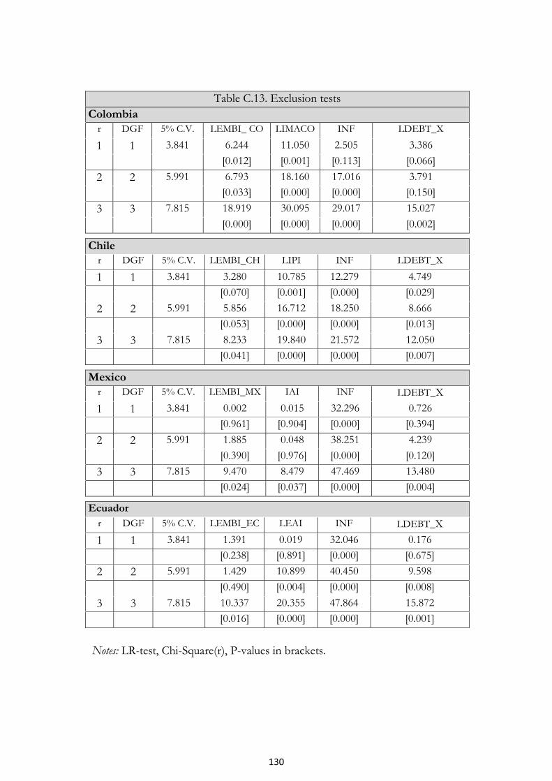
130

Table C.13. Exclusion tests

Colombia

r DGF 5% C.V. LEMBI_ CO LIMACO INF LDEBT_X 1 1 3.841 6.244 11.050 2.505 3.386 [0.012] [0.001] [0.113] [0.066] 2 2 5.991 6.793 18.160 17.016 3.791 [0.033] [0.000] [0.000] [0.150] 3 3 7.815 18.919 30.095 29.017 15.027 [0.000] [0.000] [0.000] [0.002]

Chile

r DGF 5% C.V. LEMBI_CH LIPI INF LDEBT_X 1 1 3.841 3.280 10.785 12.279 4.749 [0.070] [0.001] [0.000] [0.029] 2 2 5.991 5.856 16.712 18.250 8.666 [0.053] [0.000] [0.000] [0.013] 3 3 7.815 8.233 19.840 21.572 12.050 [0.041] [0.000] [0.000] [0.007]

Mexico

r DGF 5% C.V. LEMBI_MX IAI INF LDEBT_X 1 1 3.841 0.002 0.015 32.296 0.726 [0.961] [0.904] [0.000] [0.394] 2 2 5.991 1.885 0.048 38.251 4.239 [0.390] [0.976] [0.000] [0.120] 3 3 7.815 9.470 8.479 47.469 13.480 [0.024] [0.037] [0.000] [0.004]

Ecuador

r DGF 5% C.V. LEMBI_EC LEAI INF LDEBT_X 1 1 3.841 1.391 0.019 32.046 0.176 [0.238] [0.891] [0.000] [0.675] 2 2 5.991 1.429 10.899 40.450 9.598 [0.490] [0.004] [0.000] [0.008] 3 3 7.815 10.337 20.355 47.864 15.872 [0.016] [0.000] [0.000] [0.001]

Notes: LR-test, Chi-Square(r), P-values in brackets.

131

Table C.13. Exclusion tests

Panama r DGF 5% C.V. LEMBI_PANA LREV_C INF LDEBT_X 1 1 3.841 1.318 2.971 11.776 10.982 [0.251] [0.085] [0.001] [0.001] 2 2 5.991 11.760 13.278 20.549 15.019 [0.003] [0.001] [0.000] [0.001] 3 3 7.815 25.313 25.599 34.818 29.224 [0.000] [0.000] [0.000] [0.000]

Notes: LR-test, Chi-Square(r), P-values in brackets.

132

Annex D

Fig. D.1. Impulse responses

Legend: _____ SVEC Impulse Reponses ------- 95% Hall Percentile (B = 2000, h = 32)

133

Fig. D.2. The impulse response functions for the two permanent shocks and transitory shocks.

134

ª Standard deviations are in parentheses and t-values are in brackets.

Table D.2. Structural VEC Estimation Results. Coefficients of the B matrixª.

Variables

d(d1_cpi_log) d(reer_log) d(RIDL_log) d(oil_log)

d(d1_cpi_log)

0.0030

(0.0010)

[2.9849]

-0.0001 (0.0016) [-0.0469]

-0.0015 (0.0019) [-0.8182]

-0.0004 (0.0022) [-0.1888]

d(reer_log)

-0.0023 (0.0032) [-0.7092]

0.0072

(0.0018)

[3.9321]

0.0000 (0.0000) [0.0000]

0.0054

(0.0023)

[2.3157]

d(RIDL_log)

0.0238 (0.0308) [0.7710]

0.0175 (0.0277) [0.6324]

0.0798

(0.0256)

[3.1217]

-0.0042 (0.0152) [-0.2733]

d(oil_log)

0.0096 (0.0285) [0.3385]

-0.0210 (0.0205) [-1.0237]

0.0148 (0.0239) [0.6188]

0.0752

(0.0246)

[3.0551]

ª Bootstrap standard errors are in parentheses and bootstrap t-values are in brackets.

Table D.1. VECM Estimation Results Loading coefficientsª

d(d1_cpi_log) d(reer_log) d(RIDL_log) d(oil_log) -0.524 0.3 -4.122 -1.671 (0.049) (0.132) (1.209) (1.136)

[-10.789] [2.985] [-3.410] [-1.471] Coefficients of the cointegrating vector* (ec1(t-1))

d1_cpi_log(t-1) eer_log (t-1) d(RIDL_log) d(oil_log) 1.000 -0.089 0.001 0.009

(0.000) (0.012) (0.004) (0.004) [0.000] [-7.537] [0.242] [2.495]

135

Table D.3. Coefficients of the long run impact matrix .

Variables d(d1_cpi_log) d(reer_log) d(RIDL_log) d(oil_log)

d(d1_cpi_log)

0.0000 (0.0000) [0.0000]

0.0024

(0.0011)

[2.1669]

-0.0009 (0.0015) [-0.5539]

0.0009 (0.0041) [0.2154]

d(reer_log)

0.0000 (0.0000) [0.0000]

0.0274

(0.0126)

[2.1803]

-0.0090 (0.0171) [-0.5252]

0.0197 (0.0561) [0.3507]

d(RIDL_log)

0.0000 (0.0000) [0.0000]

0.0038 (0.0224) [0.1718]

0.0562

(0.0277)

[2.0276]

0.0495 (0.1093) [0.4526]

d(oil_log)

0.0000 (0.0000) [0.0000]

0.0000 (0.0000) [0.0000]

0.0000 (0.0239) [0.0000]

0.0876 (0.1529) [0.5728]

Notes: This is a B-model with long-run restrictions. With long-run restrictions providing five independent restrictions and one contemporaneous restriction providing one additional restriction, the Structural VAR is just identified. ML Estimation, Scoring Algorithm (see Amisano and Giannini, 1992). Convergence after 11 iterations. Log Likelihood: 1791.3097. Std-Errors are in parenthesis and t-values in brackets.

136

Table D.4. SVEC Forecast error variance decomposition of "d1_cpi_log"

Forecast Horizon d1_cpi_log reer_log RIDL_log oil_log

1 0.78 0.00 0.20 0.01

2 0.76 0.00 0.23 0.01

3 0.67 0.08 0.24 0.01

4 0.61 0.14 0.24 0.01

5 0.55 0.20 0.22 0.03

6 0.50 0.27 0.20 0.03

7 0.46 0.31 0.18 0.05

8 0.42 0.37 0.15 0.05

9 0.39 0.41 0.14 0.06

10 0.36 0.44 0.14 0.06

11 0.33 0.47 0.13 0.06

12 0.30 0.50 0.14 0.06

13 0.27 0.53 0.13 0.06

14 0.25 0.55 0.13 0.06

15 0.23 0.57 0.13 0.06

16 0.22 0.59 0.13 0.06

17 0.20 0.61 0.13 0.07

18 0.19 0.62 0.12 0.07

137

Table D.5. Just identifying restriction imposed on the 2nd beta vector and the 3H imposed on the first one.

^

1� ^

2�

tlrev 0 1

tlorev -0.881 0

[-16.317]

g tl ov 1 -0.541

[-15.866]

tleai 0 -0.636

[-6.783]

^1�

^1�

tlrev -0.006 -0.878

[-0.148] [-6.281]

tlorev 0.359 0.101

[3.466] [0.274]

g tl ov -0.102 0.290

[-2.572] [2.074

tleai -0.011 0.151

[-0.424] [1.624]

Notes: t-values in brackets.

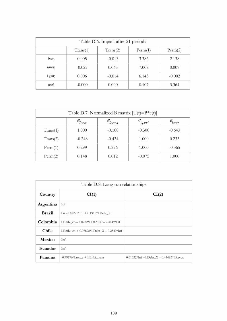
138

Table D.6. Impact after 21 periods

Trans(1) Trans(2) Perm(1) Perm(2)

tlrev 0.005 -0.013 3.386 2.138

tlorev -0.027 0.065 7.008 0.007

g tl ov 0.006 -0.014 6.143 -0.002

tleai -0.000 0.000 0.107 3.364

Table D.7. Normalized B matrix [U(t)=B*e(t)]

lrevte lorevte lgovte leaite

Trans(1) 1.000 -0.108 -0.300 -0.643

Trans(2) -0.248 -0.434 1.000 0.233

Perm(1) 0.299 0.276 1.000 -0.365

Perm(2) 0.148 0.012 -0.075 1.000

Table D.8. Long run relationships

Country CI(1) CI(2)

Argentina Inf

Brazil Lii - 0.18221*Inf + 0.1918*LDebt_X

Colombia LEmbi_co – 1.0232*LIMACO – 2.4449*Inf

Chile LEmbi_ch + 0.07898*LDebt_X – 0.2549*Inf

Mexico Inf

Ecuador Inf

Panama -0.79176*Lrev_c +LEmbi_pana 0.61532*Inf +LDebt_X – 0.44483*LRev_c

139

Table D.9a. Argentina

Equation

Variable

DLEmbi_arg DLeai Dinf DLDebt_X

DLEmbi_arg_1

0.4745

(0.0729)

[6.51]

0.055

(0.0178)

[3.11]

0.0650 (0.2797) [0.233]

-0.2536

(0.084)

[-3.02]

DLeai_1 0.2267

(0.4613) [0.492]

-0.0911 (0.1127) [-0.809]

1.5977 (1.769) [0.903]

0.386 (0.5317) [0.727]

Dinf_1

-0.00607 (0.0142) [-0.426]

-0.0024 (0.0034) [-0.697]

-0.1776

(0.054)

[-3.35]

0.0097 (0.0164) [0.593]

DLDebt_X_1

0.1185 (0.0876) [1.40]

0.0264 (0.0207) [1.28]

-0.3997 (0.3251) [-1.23]

-0.1450 (0.097) [-1.48]

CI(1)_1*

0.00036 (0.0111) [0.0329]

0.00144 (0.00272) [0.531]

-0.3642

(0.0427)

[-8.53]

-0.0088 (0.0128) [-0.69]

Dum0111p

-0.2780

(0.0689)

[-4.03]

-0.0154 (0.01683) [-0.917]

-0.1857 (0.2643) [-0.703]

-0.0372 (0.079) [-0.469]

Dum0202p

0.0959 (0.07146)

[1.34]

0.0027 (0.0174) [0.155]

1.2090

(0.2740)

[4.41]

-0.0299 (0.082) [-0.364]

Dum0204p

-0.0425 (0.0707) [-0.602]

0.022 (0.01728)

[1.30]

3.9607

(0.2713)

[14.6]

0.0106 (0.081) [0.13]

Dum0504p

-0.1002 (0.0694) [-1.44]

0.0100 (0.0169) [0.595]

-0.5195 (0.2663) [-1.95]

-0.409

(0.080)

[-5.12]

Dum0810p

-0.4681

(0.0688)

[-6.80]

0.0077 (0.01682) [0.459]

0.0541 (0.2641) [0.205]

0.073 (0.079) [0.92]

Notes: Std-Error are in parenthesis and t-values in brackets. *Argentina: CI(1) = Inf.

140

Table D.9b. Brazil

Equation

Variable DLEmbi_br DLii Dinf DLDebt__X

DLEmbi_br_1

0.2413

(0.0973)

[2.48]

-0.3561

(0.1324)

[-2.69]

-0.3595 (0.3639) [-0.988]

0.6114

(0.2551)

[2.40]

DLEmbi_br_2

-0.0300 (0.0999) [-0.301]

0.1743 (0.1359) [1.28]

-0.4834 (0.3735) [-1.29]

0.1667 (0.2618) [0.637]

DLii_1

0.0568 (0.0564) [1.01]

-0.1524

(0.0768)

[-1.98]

-0.4626

(0.2112)

[-2.19]

-0.2911

(0.148)

[-1.97]

DLii_2

0.0645 (0.0904) [0.714]

0.4152

(0.1230)

[3.37]

-0.3957 (0.3381) [-1.17]

-0.9867

(0.2371)

[-4.16]

Dinf_1

-0.0102 (0.0226) [-0.451]

-0.0114 (0.0308) [-0.372]

-0.3567

(0.0848)

[-4.21]

-0.0522 (0.0594) [-0.879]

Dinf_2

0.0392 (0.0209) [1.88]

-0.0917

(0.0284)

[-3.23]

-0.1435 (0.0781) [-1.84]

0.0879 (0.0548) [1.60]

DLDebt_X_1

0.0054 (0.0403) [0.136]

-0.0691 (0.0592) [-1.26]

0.0793 (0.1509) [0.526]

-0.3450

(0.1058)

[-3.26]

DLDebt_X_2

0.0655 (0.0447) [1.47]

0.0508 (0.0608) [0.837]

0.0320 (0.1671) [0.192]

-0.2745

(0.1171)

[-2.34]

CI (1)_1*

-0.0007 (0.0440) [-0.0172]

-0.2942

(0.0598)

[-4.91]

0.3610

(0.1646)

[2.19]

0.1442 (0.1154) [1.25]

CI (1)_2*

-0.0605 (0.0516) [-1.17]

-0.1305 (0.0702) [-1.86]

0.7434

(0.1930)

[3.85]

0.4920

(0.1353)

[3.64]

Dum0211p

0.1891

(0.0456)

[4.15]

-0.0553 (0.0620) [-0.893]

1.1154

(0.1705)

[6.54]

0.2762

(0.1196)

[2.31]

141

Table D.9b. Brazil (Continued)

Equation

Variable DLEmbi_br DLii Dinf DLDebt__X

Dum0810p

-0.1312

(0.0436)

[-3.01]

0.0228 (0.0593) [0.385]

0.0279 (0.1630) [0.171]

0.0769 (0.1143) [0.674]

Notes: Std-Errors are in parenthesis and t-values in brackets.*Brazil: CI(1) = Lii - 0.18221*Inf + 0.1918*LDebt_X.

Table D.9c. Colombia

Equation

Variable DLEmbi_co DLIMACO Dinf DLDebt_X

DLEmbi_co_1

0.1520 (0.095) [1.60]

1.1126

(0.5134)

[2.17]

-1.15585 (0.7058) [-1.64]

-0.4547 (0.3327) [-1.37]

DLIMACO_1

-0.01669

(0.008016)

[-2.08]

-0.5392

(0.0433)

[-12.5]

0.037718 (0.05953) [0.634]

-0.02614 (0.02806) [-0.932]

Dinf_1

0.01621 (0.01507)

[1.08]

0.1390 (0.06141)

[1.71]

-0.184651 (0.1119) [-1.65]

-0.03471 (0.0527) [-0.658]

DLDebt_X_1

0.01487 (0.02810) [0.501]

-0.3494

(0.1518)

[-2.30]

-0.097537 (0.2087) [-0.467]

-0.4635

(0.09839)

[-4.71]

CI(1)_1*

-0.00061 (0.00306) [-0.202]

0.1247

(0.01655)

[7.54]

0.03288 (0.02275)

[1.45]

-0.005683 (0.01072)

[-0.53]

Dum0405p

-0.1057

(0.02889)

[-3.66]

0.02470 (0.1561) [0.158]

0.16086 (0.2145) [0.75]

0.00572 (0.1011) [0.0566]

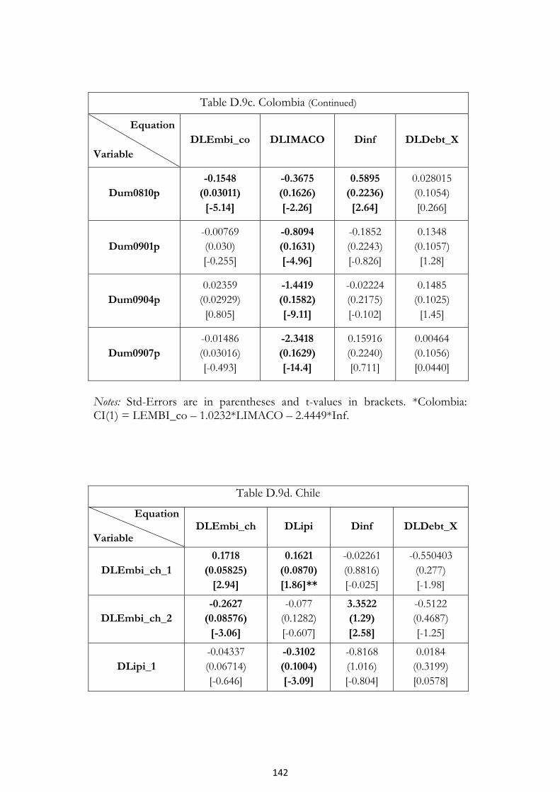
142

Table D.9c. Colombia (Continued)

Equation

Variable

DLEmbi_co DLIMACO Dinf DLDebt_X

Dum0810p

-0.1548

(0.03011)

[-5.14]

-0.3675

(0.1626)

[-2.26]

0.5895

(0.2236)

[2.64]

0.028015 (0.1054) [0.266]

Dum0901p

-0.00769 (0.030) [-0.255]

-0.8094

(0.1631)

[-4.96]

-0.1852 (0.2243) [-0.826]

0.1348 (0.1057) [1.28]

Dum0904p

0.02359 (0.02929) [0.805]

-1.4419

(0.1582)

[-9.11]

-0.02224 (0.2175) [-0.102]

0.1485 (0.1025) [1.45]

Dum0907p

-0.01486 (0.03016) [-0.493]

-2.3418

(0.1629)

[-14.4]

0.15916 (0.2240) [0.711]

0.00464 (0.1056) [0.0440]

Notes: Std-Errors are in parentheses and t-values in brackets. *Colombia: CI(1) = LEMBI_co – 1.0232*LIMACO – 2.4449*Inf.

Table D.9d. Chile

Equation

Variable DLEmbi_ch DLipi Dinf DLDebt_X

DLEmbi_ch_1

0.1718

(0.05825)

[2.94]

0.1621

(0.0870)

[1.86]**

-0.02261 (0.8816) [-0.025]

-0.550403 (0.277) [-1.98]

DLEmbi_ch_2

-0.2627

(0.08576)

[-3.06]

-0.077 (0.1282) [-0.607]

3.3522

(1.29)

[2.58]

-0.5122 (0.4687) [-1.25]

DLipi_1

-0.04337 (0.06714) [-0.646]

-0.3102

(0.1004)

[-3.09]

-0.8168 (1.016) [-0.804]

0.0184 (0.3199) [0.0578]

143

Table D.9d. Chile (Continued) Equation

Variable DLEmbi_ch DLipi Dinf DLDebt_X

DLipi_2

0.0069 (0.0639) [0.108]

-0.02408 (0.09564) [-0.252]

-2.6025

(0.9682)

[-2.69]

-0.153 (0.3049) [-0.505]

Dinf_1

0.01954 (0.022) [1.74]

0.01473 (0.0168) [0.877]

-0.2675 (0.17) [ 1.57]

-0.1225

(0.05354)

[-2.29]

Dinf_2

-0.001122 (0.0068) [-0.165]

0.00672 (0.01017) [0.661]

-0.3613

(0.1030)

[-3.51]

-0.0704

(0.03242)

[-2.17]

DLDebt_X_1

-0.0137 (0.02486) [-0.552]

-0.02618 (0.037) [-0.704]

-0.1056 (0.3762) [-0.281]

-0.6269

(0.1185)

[-5.29]

DLDebt_X_2

-0.0063 (0.02455) [-0.259]

0.03496 (0.0367) [0.953]

-0.1842 (0.3715) [-0.496]

-0.3492

(0.1170)

[-2.99]

CI(1)_1*

0.07855

(0.02832)

[2.77]

0.07911 (0.0423) [1.87]

0.0655 (0.4286) [0.153]

-0.300 (0.1349) [-2.23]

CI(1)_2*

-0.0864

(0.028)

[-3.09]

-0.07724 (0.04188)

[-1.84]

0.02834 (0.4239) [0.0669]

0.2684

(0.1335)

[2.01]

Dum0405p

-0.0995

(0.02329)

[-4.27]

-0.0123 (0.0348) [-0.355]

0.0668 (0.3524) [0.190]

-0.0393 (0.111) [-0.354]

Dum0810p

-0.1611

(0.02449)

[-6.58]

-0.01164 (0.0366) [-0.318]

0.0174 (0.3706) [0.0470]

0.1631 (0.1167) [1.40]

Dum0901p

-0.0058 (0.02581) [-0.225]

-0.2303

(0.0385)

[-5.97]

-0.5219 (0.3906) [-1.34]

0.1623 (0.1230) [1.32]

Notes: Std-Errors are in parentheses and t-values in brackets. *Chile: CI(1) = LEMBI_ch + 0.07898*LDebt_X – 0.2549*Inf . **When non-significant dummies were excluded this coefficient becomes significant.

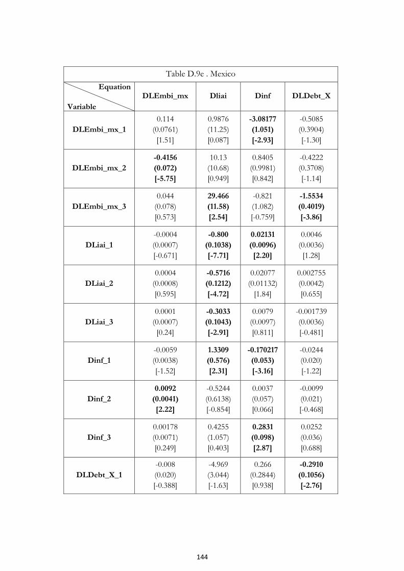
144

Table D.9e . Mexico Equation

Variable

DLEmbi_mx Dliai Dinf DLDebt_X

DLEmbi_mx_1

0.114 (0.0761) [1.51]

0.9876 (11.25) [0.087]

-3.08177

(1.051)

[-2.93]

-0.5085 (0.3904) [-1.30]

DLEmbi_mx_2

-0.4156

(0.072)

[-5.75]

10.13 (10.68) [0.949]

0.8405 (0.9981) [0.842]

-0.4222 (0.3708) [-1.14]

DLEmbi_mx_3

0.044 (0.078) [0.573]

29.466

(11.58)

[2.54]

-0.821 (1.082) [-0.759]

-1.5534

(0.4019)

[-3.86]

DLiai_1

-0.0004 (0.0007) [-0.671]

-0.800

(0.1038)

[-7.71]

0.02131

(0.0096)

[2.20]

0.0046 (0.0036) [1.28]

DLiai_2

0.0004 (0.0008) [0.595]

-0.5716

(0.1212)

[-4.72]

0.02077 (0.01132)

[1.84]

0.002755 (0.0042) [0.655]

DLiai_3

0.0001 (0.0007) [0.24]

-0.3033

(0.1043)

[-2.91]

0.0079 (0.0097) [0.811]

-0.001739 (0.0036) [-0.481]

Dinf_1

-0.0059 (0.0038) [-1.52]

1.3309

(0.576)

[2.31]

-0.170217

(0.053)

[-3.16]

-0.0244 (0.020) [-1.22]

Dinf_2

0.0092

(0.0041)

[2.22]

-0.5244 (0.6138) [-0.854]

0.0037 (0.057) [0.066]

-0.0099 (0.021) [-0.468]

Dinf_3

0.00178 (0.0071) [0.249]

0.4255 (1.057) [0.403]

0.2831

(0.098)

[2.87]

0.0252 (0.036) [0.688]

DLDebt_X_1

-0.008 (0.020) [-0.388]

-4.969 (3.044) [-1.63]

0.266 (0.2844) [0.938]

-0.2910

(0.1056)

[-2.76]

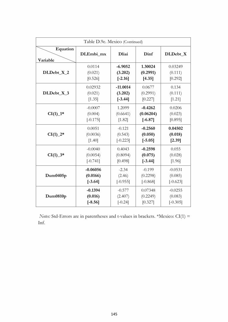
145

Table D.9e. Mexico (Continued) Equation

Variable

DLEmbi_mx Dliai Dinf DLDebt_X

DLDebt_X_2

0.0114 (0.021) [0.526]

-6.9052

(3.202)

[-2.16]

1.30024

(0.2991)

[4.35]

0.03249 (0.111) [0.292]

DLDebt_X_3

0.02932 (0.021) [1.35]

-11.0014

(3.202)

[-3.44]

0.0677 (0.2991) [0.227]

0.134 (0.111) [1.21]

CI(1)_1*

-0.0007 (0.004) [-0.175]

1.2099 (0.6641) [1.82]

-0.4262

(0.06204)

[-6.87]

0.0206 (0.023) [0.895]

CI(1)_2*

0.0051 (0.0036) [1.40]

-0.121 (0.543) [-0.223]

-0.2560

(0.050)

[-5.05]

0.04502

(0.018)

[2.39]

CI(1)_3*

-0.0040 (0.0054) [-0.741]

0.4043 (0.8094) [0.498]

-0.2598

(0.075)

[-3.44]

0.055 (0.028) [1.96]

Dum0405p

-0.06056

(0.0166)

[-3.64]

-2.34 (2.46)

[-0.955]

-0.199 (0.2298) [-0.868]

-0.0531 (0.085) [-0.623]

Dum0810p

-0.1394

(0.016)

[-8.56]

-0.577 (2.407) [-0.24]

0.07348 (0.2249) [0.327]

-0.0255 (0.083) [-0.305]

Notes: Std-Errors are in parentheses and t-values in brackets. *Mexico: CI(1) = Inf.

146

Table D.9f. Ecuador Equation

Variable DLEmbi_ec DLeai Dinf DLDebt_X

DLEmbi_ec_1

0.2528

(0.072)

[3.50]

-0.086 (0.1061) [-0.819]

-0.0027 (0.0039) [-0.700]

-0.2698

(0.1149)

[-2.35]

DLeai_1

-0.031 (0.0604) [-0.527]

-0.6107

(0.088)

[-6.88]

-0.0080

(0.0033)

[-2.42]

0.0937 (0.096) [0.0976]

Dinf_1

1.0619 (1.017) [1.04]

-0.1161 (1.493) [-0.077]

-0.1312

(0.055)

[-2.35]

-1.504 (1.616) [-0.931]

DLDebt_X_1

0.125

(0.0613)

[2.04]

-0.0820 (0.089) [-0.911]

0.0009 (0.0033) [0.273]

-0.2481

(0.097)

[-2.55]

CI(1)_1*

-0.6925 (1.073) [-0.645]

0.0627 (1.575) [0.0399]

-0.4235

(0.059)

[-7.17]

-0.7155 (1.705) [-0.42]

Dum0109p

0.0125

(0.0569)

[0.221]

0.0596 (0.083) [0.714]

0.013

(0.0031)

[4.22]

-0.089 (0.09)

[-0.987]

Dum0301p

0.083 (0.056) [1.46]

0.0077 (0.083) [0.0931]

0.017

(0.0031)

[5.43]

0.0109 (0.09) [0.121]

Dum0810p

-0.4618

(0.058)

[-7.93]

-0.1432 (0.0854) [-1.68]

-0.0047 (0.0032) [-1.49]

0.200

(0.092)

[2.16]

Dum0811p

-0.4984

(0.065)

[-7.62]

-0.0083 (0.096) [-0.08]

-0.0071 (0.0035) [-1.97]

0.0721

(0.1039)

[0.69]

Dum0906p

0.1389

(0.056)

[2.46]

-0.0377 (0.082) [-0.455]

-0.0007 (0.0031) [-0.257]

-0.410

(0.089)

[-4.92]

Notes: Std-Errors are in parentheses and t-values in brackets. *Ecuador: CI(1) = Inf_1.

147

Table D.9g. Panama

Equation

Variable

DLEmbi_pa

DLrev_c

Dinf

DLDebt_X

DLEmbi_pa_1

0.2995

(0.074)

[4.00]

0.04671 (0.1630) [0.287]

3.8661

(1.595)

[2.42]

-0.4881 (0.6171) [-0.791]

DLrev_c_1

-0.0387 (0.0456) [-0.849]

-0.1722 (0.0992) [-1.74]

0.7122 (0.9714) [0.733]

0.1170 (0.3757) [0.311]

Dinf_1

-0.0058 (0.0043) [-1.33]

-0.0228

(0.0095)

[-2.40]

-0.2284

(0.093)

[-2.45]

0.0769

(0.036)

[2.14]

DLDebt_X_1

-0.00147 (0.01302) [-0.113]

0.0337 (0.02832)

[1.19]

0.6640

(0.2772)

[2.40]

-0.0085 (0.1072) [-0.919]

CI(1)_1*

-0.0988

(0.028)

[-3.51]

0.1816

(0.0612)

[2.97]

-0.0633 (0.5992) [-0.106]

-0.1927 (0.2318) [-0.832]

CI(2)_1*

0.0067 (0.0092) [0.737]

0.00694 (0.0200) [0.346]

-0.9952

(0.1964)

[-5.07]

-0.2118

(0.0759)

[-2.79]

Dum0401p

0.02503 (0.02011)

[1.25]

-0.00535 (0.0437) [-0.122]

-1.9271

(0.4283)

[-4.50]

0.3987

(0.1656)

[2.41]

Dum0810p

-0.1819

(0.0202)

[-8.99]

0.0221 (0.044) [0.0502]

-0.4506 (0.4310) [-1.05]

0.1666 (0.1667) [1.00]

Notes: Std-Errors are in parentheses and t-values in brackets. *Panama: CI(1) = -0.79176*Lrev_c +LEmbi_pana and CI(2)=0.61532*Inf +LDebt_X – 0.44483*Lrev_c

148

Table. D.10. Comparative Analysis with only the significant coefficients

Variable Argentina Brazil Colombia Chile Mexico Ecuador Panama

Dependent Variable: DLEMBI_specific country

DLEMBI X X X X X X

DLEAI X

DINF X

DLDEBT_X X

DUM0810 X X X X X X X

DUM0405 X X X

CI() X X(CI(1))

Dependent Variable: DLEAI*

DLEMBI X X X X** X

DLEAI X X X X X

DINF X X X

DLDEBT_X X X

DUM0810 X

DUM0901 X X

CI() X X X(CI(1))

Dependent Variable: DINF

Variable Argentina Brazil Colombia Chile Mexico Ecuador Panama

DLEMBI X X X

DLEAI X X X X

DINF X X X X X X

DLDEBT_X X X

149

Table. D.10. Comparative Analysis with only the significant coefficients

Variable Argentina Brazil Colombia Chile Mexico Ecuador Panama

Dependent Variable: DINF (Continued)

DUM0810 X

CI() X X X X X(CI(2))

Dependent Variable: LDEBT_X

DLEMBI X X X

DLEAI X

DINF X X

DLDEBT_X X X X X X

DUM0810 X

CI() X X X X(CI(2))

Notes: The results shown are the ones obtained when non-significant dummies were eliminated. CI(): Specifies only the variables included in each long run relationship, which are described in Table 8. *This variable changes depending on the country. See Table 4. **When non-significant dummies were excluded this coefficient becomes significant.

150

Chapter 5 Concluding Remarks

This thesis has provided a broad analysis of three central questions associated with full dollarization, one of the fixed exchange rate regimes that has been adopted by small Latin American countries, including Ecuador, in their recent history. Specifically, it has called into doubt some of the advantages of this ERR. The analysis has centered on three specific issues: (1) the possible increase in the pass-through in Ecuador due to the change in the make-up of its trading partners other than the United States or countries pegged to the US dollar (Chapter 2); (2) the challenge faced by the fiscal policy of a dollarized, emerging country, such as Ecuador, in its attempts to achieve sustainability, given that its policymakers have a limited margin of maneuver to promote expansive policies aimed at developing the economy and improving income distribution (Chapter 3); and (3) the interdependence between fundamentals and the evolution of the Emerging Markets Bond Index (EMBI), a financial variable that serves as a barometer of the country risk premium (Chapter 4). In that chapter, I examine six Latin American countries (five of them are non-dollarized countries and one is dollarized) in addition to Ecuador, in order to identify whether exchange rate regimes play a role in the aforementioned interdependence. This concluding chapter seeks to provide a summary of the principal findings and implications of each separate study. The study of the pass-through in Ecuador shows that the trade gains under dollarization – identified in the Introduction as a potential benefit – might be finite. The emergence of a trading partner such as Brazil, a member of the association known as BRICS113, which might come to represent a large proportion of Ecuadorian imports; or the presence of new international economic organizations such as ALBA-TCP114, which excludes the United States from its commercial agreements, have the potential to bring about major changes in the make-up of Ecuador’s trading partners. Such changes might discourage trade

113 BRICS is the acronym for an association of five major emerging national economies: Brazil, Russia, India, China and South Africa. 114 The Bolivarian Alliance for the Peoples of Our America - Peoples’ Trade Treaty (ALBA-TCP) is an integration platform for the countries of Latin America and the Caribbean.

151

denominated in US dollars in periods when the exchange rate is appreciated, and consequently, they may contribute to the emergence of inflationary pressures. The empirical exercise conducted provides the following results for Ecuador: real effective exchange rate depreciations increase inflation for about twenty periods, with a maximal response after two years, while the real effective exchange rate follows oil price trends. After dollarization, the real effective exchange rate fell reaching a minimum in 2003:M5. However, after that date this trend was reversed, with oil prices increasing with the exception of 2009:M1 and 2010:M7 when oil prices experienced a downturn. Currently, as long as emerging countries such as South Korea and Brazil continue to increase their participation in Ecuadorian trade and as their currencies become more important than the US dollar in the Ecuadorian balance sheet: the higher the real effective exchange rate rise, the greater the inflationary pressures attributable to higher pass-through in Ecuador. It is my belief that the inflationary effect described in Chapter 2 would have been even stronger had I included China in the real effective exchange rate calculations, given that China is the emerging country par excellence. However, due to its relatively new flexible exchange rate regime, the decision was taken to postpone the study of this country to a later date. The outcomes obtained from this first analysis raised a number of frequently debated questions in the literature on dollarization: Should Ecuador abandon its fixed ERR? Should it have its own currency instead of the US dollar as legal tender? Are there other alternatives, such as a currency union among Latin American countries that share a common culture and language, and a similar structure of imports and exports, business cycles, and investors? These questions have been the focus of a large branch of the literature that focuses on the likelihood of Latin American countries creating a currency union similar to the European Monetary and Economic Union (see Hochreiter and Siklos, 2002). Other opinions have been made known on this issue; for instance, the Nobel laureate Joseph Stiglitz claims that Ecuador should abandon the US dollar and substitute it with an Ecuadorian dollar so as to recover the lost benefits of seignioriage. The revenues from seignioriage, according

152

to Reinhart (2003), are systematically higher in countries with a high degree of dollarization than in countries with a lower degree. Since, today, currencies are no longer guaranteed by gold but rather by what each country is able to produce (i.e., their gross domestic product), I believe Ecuador may well be ready to manage its own currency, given that it is a major oil producer and this production should be sufficient to provide the required support to uphold the value of the currency. However, appropriate fiscal and monetary policies implemented by strong economic institutions would also be necessary if Ecuador were to plan its future without the US dollar and with the country’s finite oil revenues. Chapter 3 had two objectives. First, I analyzed whether the intertemporal budget constraint had been fulfilled in Ecuador since the economy was dollarized, making its fiscal policy sustainable. Second, I studied the relationships between Ecuador’s fiscal and macroeconomic variables, in order to determine whether the country was able to face future fiscal challenges. The empirical evidence shows that, since 2007, the gap between government spending and tax revenues has increased, but that since 2012 the debt-to-GDP ratio has reversed its downward trend. This chapter seeks to fill the gap in the literature regarding the study of these kinds of issues in Ecuador, a country that, not only has a dollarized exchange rate regime, but which is also highly dependent on its volatile oil export revenues due to price fluctuations. The empirical results suggest that Ecuador’s tax revenues are not sufficient to achieve a balanced budget and the country is dependent on its oil revenues to guarantee equilibrium. Both the “additionality” and the “tax displacement” hypotheses were tested and confirmed. Thus, on the one hand, oil revenues produced equivalent or higher government expenditure, and on the other, they represented a government disincentive to increase taxes or improve the taxation system. So, the fact of being an oil producing country (which entails easier access to foreign funds via exports) has contributed to the postponement of fiscal reforms aimed at improving the tax system. As a matter of fact, oil exports today still constitute the main fiscal revenues in Ecuador for funding economic and social policies.

Consequently, one of the advantages of dollarization identified in the Introduction, namely that a fixed ERR helps improve both monetary and

153

fiscal systems, might be frustrated in an oil exporting country. This result is in line with Calvo and Mishkin (2003) who attribute weak government incentives to implement fiscal reforms (in terms of both government transparency and fiscal flexibility in order to be able to rectify fiscal imbalances) to the ease with which governments can access borrowing abroad. In relation to the second objective set in Chapter 3, one adjusting force, tax revenues, was identified, indicating that their shocks do not have a permanent impact on the fiscal and macroeconomic variables. This result is consistent with Barro’s (1979) tax smoothing theory, but does not guarantee the fiscal sustainability of a dollarized country. Since Ecuador cannot print money, it can only acquire foreign reserves from exports, taxes and remittances, which are all dependent on the impact of both the global and domestic crisis. Ii is my contention that taxes should not be the adjusting force, but rather the driving force. Ecuador needs to diversify both its economy and tax system in order to be able to levy taxes on activities other than just oil production. In addition, it is important that these new taxes are less dependent on the business cycle, so that they can bolster up the economy in periods of crisis when Ecuador needs countercyclical policies to counteract exogenous or endogenous shocks.

Finally, Chapter 4 had two aims. First, to investigate empirically the reduced impact of some of the most important macroeconomic fundamentals on the evolution of bond returns in seven Latin American countries, measured in terms of the behavior of the benchmark applied by investors: the Emerging Markets Bond Index (EMBI), and to determine how EMBI evolution has affected macroeconomic fundamentals in these seven countries (namely, Argentina, Brazil, Colombia, Chile, Ecuador, Mexico and Panama). Second, to identify whether there are any differences between these countries attributable to their respective exchange rate regimes (given that they operate different ERRs – two, Ecuador and Panama, have a full-dollarized economy while the rest have flexible ERRs). I opted to analyze the period from 2001 through 2009, the cutoff date being chosen to avoid the influence of the outbreak of the massive global economic and financial crisis in emerging economies. I deemed it best to omit from this

154

study the data corresponding to 2010 onwards, as the crisis deserves independent analysis, given that specific adjustment policies have been implemented in all the countries under review since that date. Moreover, it is likely that the variance of both financial and macroeconomic variables will have changed after 2010, giving rise to the need to analyze each period separately and to employ different econometric techniques to those used in this thesis. Undoubtedly, the extension of this analysis to the crisis period constitutes a highly relevant subject for further research. The main findings of this last Chapter can be summarized as follows. First, economic activity is only affected by the EMBI in the non-dollarized countries. This result points to another advantage of dollarization that could be added to the list in the literature. Since the empirical evidence here suggests that dollarized economies are less exposed to investors’ sentiments in the short run than they are to fundamentals, dollarization may contribute to isolate their economic activity from the broader evolution of the emerging market debt benchmark: the EMBI. Second, a country does not need to be dollarized to achieve stable levels of inflation. In the long run, non-dollarized countries with inflation targeting policies achieve similar levels of inflation to those obtained by their dollarized counterparts. This result is consistent with those presented by other authors [see, for instance, Bernanke and Mishkin (1997) and Bernanke et al. (1999)]. The novelty is to reach this conclusion by means of the cointegrated VAR approach which identifies long-run relationships, including a stationary inflation variable in non-dollarized countries.

Finally, I would like to highlight that there are a number of questions related to these three studies that have been left for further research. First, while Chapter 2 has focused on pass-through in Ecuador and shown that it increases when countries such as Brazil and South Korea are included in the analysis, it would be of particular interest to examine whether the pass-through effect increases when China is included in the real effective exchange rate calculation, since its share of world trade is increasing all the time and its exchange rate regime has become more flexible since 2005. Likewise, Chapter 3 raises some important questions regarding fiscal sustainability in other Latin American countries. For instance, the “tax displacement” hypothesis that was tested here for the Ecuadorian case might

155

also be examined for neighboring countries to identify which variable hampers the optimal development and performance of their tax systems. All developing countries face major difficulties in increasing their taxes but, given that they are necessary to rectify fiscal imbalances, it would be a very interesting subject to examine in future research.

The last – but by no means the least important – topic of interest that might be explored is related to the study conducted in Chapter 4 and the examination of the interdependence between fundamentals and financial variables in Latin American countries since the outbreak of the current global crisis. A large body of literature has studied the effects of past crises on emerging economies: including, the Russian crisis in 1998, the Brazilian crisis in 1999, and the Asian crisis in 1997. As such, it would be interesting to undertake a comparative study of dollarized and non-dollarized countries against this backdrop of crisis, in order to continue this study of the fascinating debate that examines whether the exchange rate regime really matters.

References

Bernanke, B. S., Laubach, T., Mishkin, F. S. and Posen, A. S. (1999) Inflation Targeting: Lessons from International Experience, Princeton University Press., USA.

Bernanke, B. S. and Mishkin, F. S. (1997) Inflation Targeting: A New Framework for Monetary Policy?, Journal of Economic Perspectives, Vol. 11, Nº 2, Spring, pp. 97-116.

Hochreiter, E. and Siklos, P. L. (2002) Alternative Exchange Rate Regimes: The Options for Latin America, North American Journal of Economic and Finance 13, pp. 195-211.