essar steel minnesota modifications project - draft supplemental

Source/ Characterization

Original MSI EIS/

SDS Quantity1

Proposed ESSM Quantity

Storage, Handling and Disposal

SOLID WASTES

Construction Debris

To Be Determined

To Be Determined, slightly more based on larger buildings for pellet plant, crusher and concentrator

Construction debris waste would be generated during construction and through ongoing maintenance. Efforts would be made to recycle materials on site or through available public or private recycling programs. Essar would use a licensed demolition disposal contractor to properly handle the disposal of construction debris. The construction debris would be hauled to a licensed demolition debris landfill with an approved industrial waste management plan for acceptance of construction debris.

Municipal solid waste from offices, shops and production facilities (excluding shop and industrial wastes)

Approx 1,000 tons per year


Typical municipal solid waste (MSW) would be produced from offices and non-production-related locations (lunchrooms, control stations). A comprehensive recycling program would be implemented. A licensed hauler would dispose of MSW in a permitted solid waste landfill.

Crusher baghouse dust

Approx 4,500 tons per year1


Has the same composition as the ore and would be sent to the concentrator to be reincorporated into the process.

Concentrator baghouse dust

900 tons per year 1,700 tons per year Composed of taconite ore dust that would be reincorporated into the process.

Mill scale 36,000 metric tons per year

36,000 metric tons per year (no change in steel production)

Mill scale (primarily iron oxide) is produced by descaling hot metal strips using water jets. The wet scale is collected in the scale pit, dewatered and disposed of by landfilling or by reincorporating it back into the iron-making process. Mill scale is sometimes used as a source of iron by the Portland cement industry, and Essar will explore this option as it gets closer to operation. A beneficial use determination would be required for reuse of this material.


Original MSI EIS/

SDS Quantity1



(In-house) Scrap steel

180,000 metric tons per year


Scrap steel is produced from spillage, ladle skulls and tipped steel in the melt shop, as well as from head and tail crops and cobbles in the rolling mill. All scrap would be collected and recycled into the steelmaking process or (if not suitable for reuse) sold as commercial scrap.

Steel Mill, Straight Grate and DRI Refractory

9,000 tons per year

10,800 tons per year (no change in steel production; change is in Pellet Plant straight grate refractory)

Furnace lining (brick refractory) wears out and must be replaced on a routine maintenance cycle. Refractory waste from other facilities has indicated that this material is not hazardous. A normal refractory disposal practice is to landfill but crushing and recycling as construction aggregate will also be explored.

Slag 300,000 metric tons per year


The EAF and ladle furnaces will produce slag. Slag will be tapped into a ladle and transported to the slag handling area. There it is poured, quenched and fragmented for reprocessing. The major constituents of slag are calcium oxide, silicon oxide and iron. Slag is considered non-hazardous and is commonly used as construction material. The metallic fraction of the slag stream will be recycled at the EAFs. A contractor will be hired to manage the slag and will be responsible for removing the material, disposing it or employing the material off the project site for some other appropriate beneficial reuse. A beneficial use determination would be required for reuse of this material.

SLUDGE

Sand filter filtration sludge

To Be Determined

To Be Determined; more for Pellet Plant wastewater but no change for DRI/Steel Mill wastewater

Sand filtration of recycled process water will produce a filter backwash composed of particulates. The backwash will be thickened by sedimentation and dewatered by a belt filter producing a small amount of dewatered sludge. The sludge will be disposed of by landfilling.

Wastewater Treatment

To Be Determined

Crystallized solids from evaporation and crystallization treatment, to be disposed of at a permitted solid waste landfill.


Original MSI EIS/

SDS Quantity1



Pellet plant air scrubber sludge (different rates for wet scrubber vs. dry scrubber, both evaluated)

3,900 tons per year of softening sludge (dry); 3,000 tons per year of reverse osmosis (RO) brine (dry) from waste gas and other stack blowdown; 1,600 tons per year of iron particles

If wet scrubber: 5,300 tons per year of softening sludge (dry); 4,000 tons per year of reverse osmosis (RO) brine (dry) from waste gas and other stack blowdown; 2,200 tons per year of iron particles If dry scrubber: 1,260 tons per year solid waste from the dry scrubber baghouse; 3,000 tons per year of iron particles

For wet scrubber: composition would include filtered solids such as calcium, magnesium, chloride, fluoride, nitrate, sulfate, iron and carbonate. The softening sludge would be disposed of at a permitted solid waste landfill. For dry scrubber: composition would be primarily calcium sulfate and excess lime. A small amount of residual solids from the multiclone system would also be present. The solid waste collected in the baghouse would be disposed of at a permitted solid waste landfill.

Pellet plant multiclone air scrubber solids (present for both wet and dry scrubber designs)

90,000 tons per year1

121,000 tons per year A multi-cyclone unit would remove the larger particles and reincorporate them into the process. Expected to mirror taconite pellet composition. Sludge could be recycled to concentrator for repelletizing or sent directly to tailings basin if beneficial for reducing mercury emissions.

DRI plant air scrubber sludge

515 tons per year of RO brine (dry)


Composition would be similar to the make-up water with some ammonia, sodium, and phosphorus enrichment. The dry solids that are generated by this treatment process would be disposed of at a permitted solid waste landfill.

DRI Cooling Tower Blowdown



Composition would be similar to the make-up water with sodium and phosphorus enrichment (from chemical additives). The dry solids that are generated by this treatment process would be disposed of at a permitted solid waste landfill.

Oil Separation System

To Be Determined

To Be Determined Oily sludge to be managed by licensed disposal contractor.

Steel Mill Cooling Towers – Blowdown

1,500 tons per year (dry) of RO brine

1,500 tons per year (dry) of RO brine

Composition would be similar to the make-up water with phosphorus and sodium enrichment (from chemical additives). The dry solids that are generated by this treatment process would be disposed of at a permitted solid waste landfill.


Original MSI EIS/

SDS Quantity1



Steel mill – Scale pit sludge

To Be Determined

To Be Determined (no change in steel production)

Scale pit sludge includes oil and grease from rolling mill and fine iron oxide particles mixed with water. To be sent to a licensed commercial waste-oil disposal or commercial oil-recovery facility.

HAZARDOUS AND SPECIAL WASTES

Mine/Crusher Used Oil and Lubricants

4,000 gallons per year

7,900 gallons per year Shovels and drilling equipment would produce used lubricants and hydraulic oil. Also, see truck shop, below. Used oil would be collected and disposed of by a licensed commercial waste oil disposal contractor. Solvents would be drummed and disposed of by a licensed commercial hazardous waste disposal contractor.

Electric Arc Furnace Baghouse Dust

10,000-76,000 tons per year1

10,000-76,000 tons per year (no change in steel production)

RCRA-listed KO-61 waste; Essar may pursue declassification of its baghouse dust because virgin iron units supplied to the furnaces will not have the typical heavy metal contaminants introduced by scrap metal. Essar plans to briquette baghouse dust with the intent to recharge the material to the EAFs. Alternately, Essar will use a commercial hazardous waste contractor or recycling at the start of operations. If delisted, EAF dust would be recycled into iron/steel processes or disposed of in a local landfill.

The range of quantities provided is based on the original MSI FEIS and SDS permit application. The particulate matter calculation approach yields a range of quantities, as follows:

a) Based on the emission inventory, solid waste generation rates would be 10,000 tons per year.

b) Based on stack flow rates at 1.0 gr/dscf, solid waste generation rates would be 24,000 tons per year.

c) Based on stack flow rates, a controlled emission rate of 35 tons/year and control efficiency of 99.9%, solid waste generation rates would be 70,000 tons per year.

Maintenance – waste solvents

To Be Determined

To Be Determined Waste would be drummed and disposed of by a licensed commercial hazardous waste disposal contractor.


Original MSI EIS/

SDS Quantity1



Maintenance – waste lubricants

To Be Determined

To Be Determined Waste would be drummed and disposed of by a licensed commercial hazardous waste disposal contractor.

Paint Shop Waste 4,000 lbs per year 4,000 lbs per year The paint shop would generate small amounts of paint waste, solvents and possibly sandblasting waste. A paint booth would not be operated on-site. Waste would be drummed and disposed of by a licensed commercial hazardous waste disposal contractor.

Truck Shop Waste 1,000 gallons per year1

2,100 gallons per year The truck shop would generate used oil and smaller amounts of solvents. Used oil would be collected and disposed of by a licensed commercial used oil disposal contractor. Solvents would be drummed and disposed of by a licensed commercial hazardous waste disposal contractor. Mine vehicles would be owned, operated and maintained by a qualified contractor who would be responsible for the proper handling storage and disposal of wastes associated with the mine vehicles.

Laboratory – waste solvents and materials

300 gallons per year

400 gallons per year Waste would be drummed and disposed of by a licensed commercial hazardous waste disposal contractor.

DRI Catalyst 241 tons per change out1

241 tons per change out (no change to DRI production)

Nickel-based catalyst to be recycled by catalyst vendor. Catalyst change out is expected; however, the rate at which catalyst becomes spent can vary depending upon process upsets or malfunctions.

1Most quantities provided are from the original MSI FEIS; however, some quantities were revised for the MSI NPDES /SDS Permit. Those that were updated in the MSI Permit Application are identified by this superscript.

Each of these items is briefly described in terms of relative electrical energy use reduction compared to more energy intensive alternatives. The electrical energy use is then translated into a CO2 emission factor and associated GHG emissions savings. The CO2 emission factor used to calculate indirect CO2 emissions from electricity consumption is taken from the US EPA Emissions and Generated Resource Integrated Database (eGRID), version 2.01. Based on the location of the facility, the Midwest Reliability Organization (West) (MROW) region factors from 2005 are used (Table B-1). Table B-2 summarizes the emissions savings of the proposed Essar project. Most reductions would occur off-site at the point of power production. None of the reductions are Scope 1 (direct) reductions.

Pollutant Emission Factor (g CO2 / kWh)

Emission Factor (metric ton CO2 / MWh)

CO2 826.37 0.83

CH4 0.0127 0.000013

N2O 0.0139 0.000014

Source Estimated GHG Reduction (metric tons CO2-e per year)

Dry Cobbing 10,700

Autogenous grinding 36,900

Hydraulic Trommel 7,700

Ball Mill Transport 34,100

Gravity Transport 18,600

Ceramic Filter 24,300

Hytemp Pellet Transfer 513,000

Total Savings Associated with Project 645,300

To manage and minimize haul truck energy use Essar examined fuel sources and their reported CO2 emissions, as well as fuel feasibility based on availability, cost, and operational constraints. The feasibility factors were then subjectively evaluated to make a selection of fuel type. The fuel sources were ranked according to net emissions by using a CO2 emission factor and then considering CO2 sequestration. The summary analysis is reported in the following table.

Though the biodiesel emission factor is the largest, emissions from biodiesel combustion are considered biogenic. Unlike fossil CO2, 40% of which will still be present in the atmosphere 100 years after emission (and 10% of which will still be present in the atmosphere 10,000 years after emission), due to vegetative regrowth, most or all of CO2 emitted as a result of liquid biofuels combustion is removed from the atmosphere within a year or two. For this reason, biodiesel (typically produced from soybeans) was ranked first. TCR GRP guidance requires that CO2 emissions from biodiesel combustion be kept track of and reported separately.

Biodiesel-fueled trucks would not feasible because of limited fuel availability of biodiesel and because of operational constraints with biodiesel at low temperatures. Compressed natural gas (CNG) trucks are infeasible due to their limited availability and added cost. Natural gas fired trucks would also have higher NOx emissions which would increase visibility impacts.

Essar has committed to increasing haul truck size from the original MSI plans. This would minimize GHG emissions per ton moved due to efficiency of scale.

Dry cobbing would be used to help separate non-magnetic constituents from the processed material. When using this process in the primary grinding circuit ahead of the concentrating step, many of the nonmagnetic constituents will be removed, thereby reducing grinding requirements ahead of the concentrating step. Additionally, cobber rejects would be used for road construction, eliminating the need for an aggregate plant in the area of the mine pit. Essar Engineering has calculated that due to lower energy use, autogenous grinding will reduce energy usage by 1.8 kWh/ton of crude ore.

Additionally, cobber rejects will be used for road construction, eliminating the need for an aggregate plant in the area of the mine plant. Essar engineering has calculated that this will reduce energy usage by 10.7 kWh/ton of crude ore.

Rank Fuel CO2 Emission Factor (kg CO2 / MMBtu)

Feasible? Essar Selection

1 Biodiesel1 79.97 No No

2 Compressed Natural Gas2 53.06 No No

3 Diesel3 73.15 Yes Yes

1. Based on Factor from Table 13.1 of TCR GRP, using National Biodiesel Board heating value of 118,296 Btu/gal for B100. http://www.biodiesel.org/pdf_fles/fuefactsheets/BTU_Content_Final_Oct2005.pdf)

Note that CO2 emissions from biodiesel combustion are considered “biogenic” and reported separately. 2. Factor from Table 12.1 of TCR GRP, converted using 1,029 Btu/scf from Table 12.1. 3. “Distillate Fuel Oil No. 1 and 2” Factor from Table 13.1 of TCR GRP

http://www.biodiesel.org/pdf_fles/fuefactsheets/BTU_Content_Final_Oct2005.pdf

Dry Cobbing

Estimated Reduction


Associated GHG Savings (metric ton CO2 / yr)

12,857 MWh/yr 0.83 10,700

Autogenous grinding involves the use of coarse ore particles as media. The predominant grinding mechanism in autogenous grinding is attrition. Very little grinding is by impact. Semi-autogenous grinding is used in place of autogenous grinding when the ore does not produce the necessary competent media, typically with the use of forged steel balls.

Essar engineering has test results demonstrating that an autogenous mill will consume less energy than a semi-autogenous mill. Autogenous grinding will provide low cost comminution between crushing and final grinding operations.

Autogenous Grinding

Estimated Reduction


Associated GHG Savings (ton CO2 / yr)

37,857 MWh/yr 0.83 30,730

Essar engineering has calculated that avoidance of use of steel balls in autogenous grinding will reduce energy usage by 600 kWh/ton of steel balls. This is based on a consumption rate of 0.6 kg of steel grinding balls per m.t. of crude feed.

Elimination of Need for Forged Steel Balls in Autogenous Grinding

Estimated Reduction



7,400 MWh/yr 0.83 6,150

A Hydraulic Trommel return system will be used to convey materials, reducing the need for standard recirculating system screens and conveyors. This can be accomplished by incorporating a high pressure water jet into the process to hydraulically convey oversize back to the head of the mill. This eliminates the need for a number of scalping screens and recycle conveyors.

Essar engineering has calculated that using a hydraulic trommel instead of a standard screen and conveyor system will eliminate 7728 hours per year of screen and conveyor operations at a rate of 1200 kWh.

Hydraulic Trommel

Estimated Reduction



9,300 MWh/yr 0.83 7,700

A cyclone was initially designed for material classification in the primary ball mill area. Essar evaluated the effectiveness of screening for material classification instead of a cyclone in the screening circuit.

Using the ball mill is effective and reduces power use by 25%. Essar engineering has calculated that using a ball mill instead of a cyclone for fines transport will reduce energy usage by 2.0 kWh/ton of crude ore.

Ball Mill Transport

Estimated Reduction Emission Factor

(metric ton CO2 / MWh) Associated GHG Savings

(metric ton CO2 / yr)

37,020 MWh/yr 0.83 34,100

The initial layout of the plant assumed use of pumps to transport tails and concentrate through crushing, grinding and concentrating. During initial foundation construction activities, the topography and subsurface were found to be conducive to laying out the plant so that gravity could be further used to drive transportation of a number of these process streams. A calculation was made to determine the energy avoided in each transportation step that could be replaced by gravity flow. The table below summarizes these estimates.

Gravity Transport

Process Estimated Reduction



Flotation Concentrate to Concentrate Thickener

1,200 MWh/yr 0.83 1,030

Flotation talks to Tailings thickener

430 MWh/yr 0.83 350

Concentrate Hydroseperator overflow to Tailings thickener

8,700 MWh/yr 0.83 7,200

Concentrate Thickener overflow to Tailings thickener

930 MWh/yr 0.83 770

Tailing Hydroseperator overflow to Tailings thickener

11,100 MWh/yr 0.83 9,200

Vacuum filters were initially identified as the method to develop concentrate filter cake. Essar investigated potential options to optimize this process. A ceramic filter process using significantly smaller vacuum requirements in combination with filter back wash was determined to be appropriate for use. Essar’s evaluation found power requirements to be nearly an order of magnitude lower using this approach. Essar engineering has calculated that using a ceramic filter instead of a vacuum filter will reduce energy usage by 4.5 kWh/ton of crude ore.

Ceramic Filter




39,250 MWh/yr 0.83 24,300

The Hytemp system is the pneumatic transfer of hot DRI pellets to the EAF to save electric energy. Pellets coming off the grate are hot. The same pellets will later need to be heated during steel making. Essar has identified a process that can handle the hot pellets and transfer them to the steel plant. The DRI product enters the pneumatic system at 700°C and the DRI temperature drops approximately 120°C during transport to the EAF. The hot pellets can then be used in the process, minimizing the amount of heat and energy required to bring the pellets to steel making temperatures. The calculated savings from this process step are a decrease 0.23 MWh per metric ton of steel throughput.

Hytemp DRI Pellet Transfer




621,000 MWh/yr 0.83 513,000

The furnace is designed to fire natural gas. Other fuels are evaluated below with regard to efficiency.

The fuel options can be ranked in order of GHG emission factors (kg CO2 emitted per MMBtu):

Rank Fuel Typical CO2 Emission Factor (kg CO2 / MMBtu))

1 Biomass1 79.97

2 Natural Gas2 53.06

3 Fuel Oil3 73.15

4 Coal4 93.98

1. Wood and Wood Waste Factor from table 12.2 of TCR GRP Note that CO2 emissions from biomass combustion are considered “biogenic” and reported separately. 2. “Unspecified” Natural Gas Factor from Table 12.2 of TCR GRP.

3. Distillate Fuel Oil (#1, 2, 84) Factor from Table 12.2 of TCR GRP.

Unspecified (Other Industrial) Coal Factor from Table 12.2 of TCR GRP.

Though the biomass emission factor is the second largest, emissions from biomass combustion are considered biogenic. Unlike fossil CO2, 40% of which will still be present in the atmosphere 100 years after emission (and 10% of which will still be present in the atmosphere 10,000 years after emission), due to vegetative regrowth, most or all of CO2 emitted as a result of the combustion of solid biomass is removed from the atmosphere within 50 to 70 years. For this reason, biomass was ranked first. TCR GRP guidance recommends that CO2 emissions from biomass combustion be kept track of and reported separately.

Essar is proposing to burn natural gas exclusively. Biomass cannot be handled by the furnace burners, which are designed for maximum fuel efficiency to minimize NOx generation and subsequently GHG generation. Neither of the two other options (coal or fuel oil) is being considered because they result in higher CO2 emissions. In addition, similar to biomass, coal cannot be utilized by the furnace burners. Coal also results in higher SO2 and mercury emissions.

The proposed ESMM project is expected to require 2,649,000 MWh/yr. The pellet plant, DRI unit, and steel mill are located within the municipal boundary of the City of Nashwauk. As such they are required to purchase power from the service area provider for the City of Nashwauk and are not eligible to select an electricity provider based on MN Statute 216B.40 which states:

Except as provided in sections 216B.42 and 216B.421, each electric utility shall have the exclusive right to provide electric service at retail to each and every present and future customer in its assigned service area and no electric utility shall render or extend electric service at retail within the assigned service area of another electric utility unless the electric utility consents thereto in writing; provided that any electric utility may extend its facilities through the assigned service area of another electric utility if the extension is necessary to facilitate the electric utility connecting its facilities or customers within its own assigned service area.

Based on this Statute, customers located within a municipal boundary must purchase power from the service area provider for the municipality. The service area provider for the City of Nashwauk is the Nashwauk Public Utility Commission (PUC). The Nashwauk PUC has selected Minnesota Power for electric power for the Essar facility. However, several potential power provider emission rates as well as the MROW emission factor are provided below for comparison purposes. The calculated emissions associated with electric use are based on the Midwest Reliability Organization West (MROW) emission factor provided in the EPA’s Emissions and Generated Resource Integrated (eGRID) database.

Minnesota Electrical Provider Ranking

Rank Electricity Provider CO2 Emission Factor (lb CO2 / MWh)

1 Xcel Energy1 1,317.2

2 Alliant Energy1 1,782.2

3 MROW2 1,821.8

4 Otter Tail Power1 2,099.9

5 Minnesota Power1 2,159.5

6 Great River Energy1 2,202.2

1Warner, James. 2008. Memorandum to Affected Air Permit Applicants on Completion of a Greenhouse Gas Emissions Evaluation. MPCA July 16, 2008.

2Midwest Reliability Organization (West) average applicable region factor from 2005 (EPA egrid database http://cfpub.epa.gov/egridweb/view.cfm DOA 2/10/10)

These emission factors are based on the current mix of fuels used to produce electricity at each of these utilities, as is the MROW factor. Additional renewable energy production is expected to come on-line over time and will have an effect of lowering the emissions from all of these sources, as well as the MROW factor. Minnesota Power which is ranked 5th in the table above and is the closest power provider to the proposed ESMM project is discussed as an example of how emission rates are expected to decrease in the future.

Minnesota Power has additional renewable energy coming on line which will significantly supplement Minnesota Power’s existing hydro and wind renewable resources to bring overall renewable energy supplied to Minnesota Power customers to 25% by 2025. Minnesota Power, for example, has contracted to purchase approximately 130 MW of wind energy and is expanding its wind power operations, including installation of 32.5 MW of capacity at the end of 2008. The impact of renewable hydro generation has been reducing the Minnesota Power average CO2 emission rate by 4 to 5 percent in recent years, depending on reservoir water reserves. Most new renewable energy to meet the 25% renewable portfolio standard will be from wind energy resources, so it is expected that Minnesota Power’s CO2 emission rate will decrease uniformly in coming years. Minnesota Power expects a decrease of roughly 20% of CO2 emitted per megawatt generated by 2015. Applying a 20% decrease to the Minnesota Power CO2 emission factor lowers it to 1,727.6 lbs of CO2 / MWh. This projected decrease is not directly applicable to the existing emissions rankings illustrated above because all of the power providers are subject to Minnesota’s renewable energy standards and, therefore, will also see future decreases in emissions. It is unclear how future rankings will change. Minnesota Power’s projected 20% decrease by 2015 has not been included in the GHG emission savings calculations.

http://cfpub.epa.gov/egridweb/view.cfm

If deemed effective, Essar will consider these additional measures.

Mixing by High Intensive Vertical Eirich Mixer Instead of Horizontal Mixer The use of vertical mixers may improve efficiency and reduce energy use and GHG emissions. If deemed effective, Essar will consider use of these technologies.

Running Greenball Production using a Balling Disc Instead of a Balling Drum The use of a balling disk instead of a balling drum may improve efficiency and reduce energy use and GHG emissions.

Fuel Shipping Transportation of natural gas for use in the furnace would be via pipeline. This approach eliminates the need for motorized transport of fuel as a component of GHG emissions. However, factors like methane leakage from T&D systems have not been evaluated, and could be considerable.

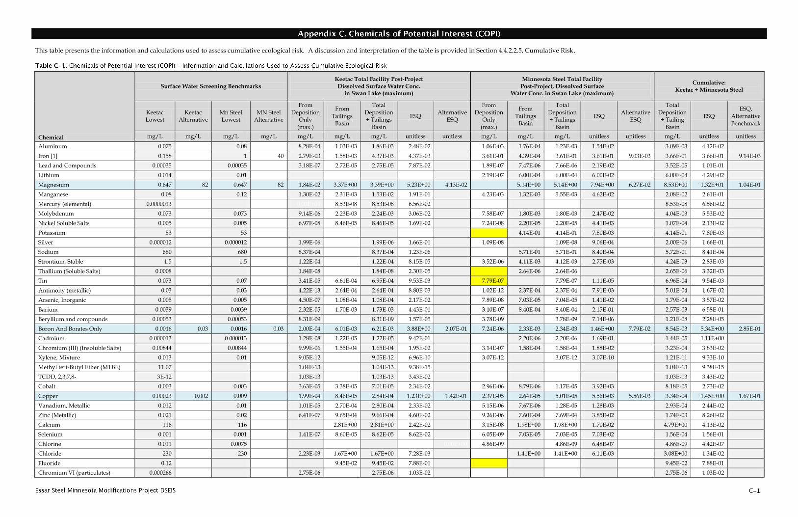
This table presents the information and calculations used to assess cumulative ecological risk. A discussion and interpretation of the table is provided in Section 4.4.2.2.5, Cumulative Risk.

Chemical

Surface Water Screening Benchmarks Keetac Total Facility Post-Project Dissolved Surface Water Conc.

in Swan Lake (maximum)

Minnesota Steel Total Facility Post-Project, Dissolved Surface

Water Conc. in Swan Lake (maximum)

Cumulative: Keetac + Minnesota Steel

Keetac Lowest

Keetac Alternative

Mn Steel Lowest

MN Steel Alternative

From Deposition

Only (max.)

From Tailings

Basin

Total Deposition + Tailings

Basin

ESQ Alternative

ESQ

From Deposition

Only (max.)

From Tailings

Basin


Basin

ESQ Alternative

ESQ

Total Deposition + Tailing

Basin

ESQ ESQ,

Alternative Benchmark

mg/L mg/L mg/L mg/L mg/L mg/L mg/L unitless unitless mg/L mg/L mg/L unitless unitless mg/L unitless unitless

Aluminum 0.075 0.08 8.28E-04 1.03E-03 1.86E-03 2.48E-02 1.06E-03 1.76E-04 1.23E-03 1.54E-02 3.09E-03 4.12E-02

Iron [1] 0.158 1 40 2.79E-03 1.58E-03 4.37E-03 4.37E-03 3.61E-01 4.39E-04 3.61E-01 3.61E-01 9.03E-03 3.66E-01 3.66E-01 9.14E-03

Lead and Compounds 0.00035 0.00035 3.18E-07 2.72E-05 2.75E-05 7.87E-02 1.89E-07 7.47E-06 7.66E-06 2.19E-02 3.52E-05 1.01E-01

Lithium 0.014 0.01 2.19E-07 6.00E-04 6.00E-04 6.00E-02 6.00E-04 4.29E-02

Magnesium 0.647 82 0.647 82 1.84E-02 3.37E+00 3.39E+00 5.23E+00 4.13E-02 5.14E+00 5.14E+00 7.94E+00 6.27E-02 8.53E+00 1.32E+01 1.04E-01

Manganese 0.08 0.12 1.30E-02 2.31E-03 1.53E-02 1.91E-01 4.23E-03 1.32E-03 5.55E-03 4.62E-02 2.08E-02 2.61E-01

Mercury (elemental) 0.0000013 0.00E+00 8.53E-08 8.53E-08 6.56E-02 0.00E+00 8.53E-08 6.56E-02

Molybdenum 0.073 0.073 9.14E-06 2.23E-03 2.24E-03 3.06E-02 7.58E-07 1.80E-03 1.80E-03 2.47E-02 4.04E-03 5.53E-02

Nickel Soluble Salts 0.005 0.005 6.97E-08 8.46E-05 8.46E-05 1.69E-02 7.24E-08 2.20E-05 2.20E-05 4.41E-03 1.07E-04 2.13E-02

Potassium 53 53 4.14E-01 4.14E-01 7.80E-03 4.14E-01 7.80E-03

Silver 0.000012 0.000012 1.99E-06 1.99E-06 1.66E-01 1.09E-08 1.09E-08 9.06E-04 2.00E-06 1.66E-01

Sodium 680 680 8.37E-04 8.37E-04 1.23E-06 5.71E-01 5.71E-01 8.40E-04 5.72E-01 8.41E-04

Strontium, Stable 1.5 1.5 1.22E-04 1.22E-04 8.15E-05 3.52E-06 4.11E-03 4.12E-03 2.75E-03 4.24E-03 2.83E-03

Thallium (Soluble Salts) 0.0008 1.84E-08 1.84E-08 2.30E-05 2.64E-06 2.64E-06 0.00E+00 2.65E-06 3.32E-03

Tin 0.073 0.07 3.41E-05 6.61E-04 6.95E-04 9.53E-03 7.79E-07 7.79E-07 1.11E-05 6.96E-04 9.54E-03

Antimony (metallic) 0.03 0.03 4.22E-13 2.64E-04 2.64E-04 8.80E-03 1.02E-12 2.37E-04 2.37E-04 7.91E-03 5.01E-04 1.67E-02

Arsenic, Inorganic 0.005 0.005 4.50E-07 1.08E-04 1.08E-04 2.17E-02 7.89E-08 7.03E-05 7.04E-05 1.41E-02 1.79E-04 3.57E-02

Barium 0.0039 0.0039 2.32E-05 1.70E-03 1.73E-03 4.43E-01 3.10E-07 8.40E-04 8.40E-04 2.15E-01 2.57E-03 6.58E-01

Beryllium and compounds 0.00053 0.00053 8.31E-09 0.00E+00 8.31E-09 1.57E-05 3.78E-09 3.78E-09 7.14E-06 1.21E-08 2.28E-05

Boron And Borates Only 0.0016 0.03 0.0016 0.03 2.00E-04 6.01E-03 6.21E-03 3.88E+00 2.07E-01 7.24E-06 2.33E-03 2.34E-03 1.46E+00 7.79E-02 8.54E-03 5.34E+00 2.85E-01

Cadmium 0.000013 0.000013 1.28E-08 1.22E-05 1.22E-05 9.42E-01 2.20E-06 2.20E-06 1.69E-01 1.44E-05 1.11E+00

Chromium (III) (Insoluble Salts) 0.00844 0.00844 9.99E-06 1.55E-04 1.65E-04 1.95E-02 3.14E-07 1.58E-04 1.58E-04 1.88E-02 3.23E-04 3.83E-02

Xylene, Mixture 0.013 0.01 9.05E-12 9.05E-12 6.96E-10 3.07E-12 3.07E-12 3.07E-10 1.21E-11 9.33E-10

Methyl tert-Butyl Ether (MTBE) 11.07 1.04E-13 1.04E-13 9.38E-15 0.00E+00 1.04E-13 9.38E-15

TCDD, 2,3,7,8- 3E-12 1.03E-13 1.03E-13 3.43E-02 0.00E+00 1.03E-13 3.43E-02

Cobalt 0.003 0.003 3.63E-05 3.38E-05 7.01E-05 2.34E-02 2.96E-06 8.79E-06 1.17E-05 3.92E-03 8.18E-05 2.73E-02

Copper 0.00023 0.002 0.009 1.99E-04 8.46E-05 2.84E-04 1.23E+00 1.42E-01 2.37E-05 2.64E-05 5.01E-05 5.56E-03 5.56E-03 3.34E-04 1.45E+00 1.67E-01

Vanadium, Metallic 0.012 0.01 1.01E-05 2.70E-04 2.80E-04 2.33E-02 5.15E-06 7.67E-06 1.28E-05 1.28E-03 2.93E-04 2.44E-02

Zinc (Metallic) 0.021 0.02 6.41E-07 9.65E-04 9.66E-04 4.60E-02 9.26E-06 7.60E-04 7.69E-04 3.85E-02 1.74E-03 8.26E-02

Calcium 116 116 2.81E+00 2.81E+00 2.42E-02 3.15E-08 1.98E+00 1.98E+00 1.70E-02 4.79E+00 4.13E-02

Selenium 0.001 0.001 1.41E-07 8.60E-05 8.62E-05 8.62E-02 6.05E-09 7.03E-05 7.03E-05 7.03E-02 1.56E-04 1.56E-01

Chlorine 0.011 0.0075 0.00E+00 4.86E-09 4.86E-09 6.48E-07 4.86E-09 4.42E-07

Chloride 230 230 2.23E-03 1.67E+00 1.67E+00 7.28E-03 1.41E+00 1.41E+00 6.11E-03 3.08E+00 1.34E-02

Fluoride 0.12 9.45E-02 9.45E-02 7.88E-01 9.45E-02 7.88E-01

Chromium VI (particulates) 0.000266 2.75E-06 2.75E-06 1.03E-02 2.75E-06 1.03E-02

Chemical






Keetac Lowest

Keetac Alternative

Mn Steel Lowest


From Deposition

Only (max.)

From Tailings

Basin


Basin

ESQ Alternative

ESQ

From Deposition

Only (max.)

From Tailings

Basin


Basin

ESQ Alternative

ESQ


Basin

ESQ ESQ,



Methyl Mercury (dissolved phase) 0.00000246 2.8E-09 4.30E-10 4.30E-10 1.75E-04 2.66E-10 2.66E-10 9.51E-02 6.96E-10 2.83E-04

Formaldehyde 0 0.0496 4.42E-06 4.42E-06 0.00E+00 0.00E+00 1.18E-05 1.18E-05 2.38E-04 1.62E-05 3.27E-04

Benzo[a]pyrene 0.000014 0.000014 8.00E-10 8.00E-10 5.71E-05 6.14E-11 6.14E-11 4.38E-06 8.61E-10 6.15E-05

Chloroform 0.0018 2.34E-13 2.34E-13 1.30E-10 2.34E-13 1.30E-10

Benzene 0.021 0.02 6.50E-11 6.50E-11 3.10E-09 6.11E-10 6.11E-10 3.05E-08 6.76E-10 3.22E-08

Trichloroethane, 1,1,1- 0.011 5.61E-14 5.61E-14 5.10E-12 5.61E-14 5.10E-12

Bromomethane 0.016 4.33E-14 4.33E-14 2.70E-12 4.33E-14 2.70E-12

Chloromethane 5.5 9.96E-14 9.96E-14 1.81E-14 9.96E-14 1.81E-14

Carbon Disulfide 0.00092 7.28E-15 7.28E-15 7.91E-12 7.28E-15 7.91E-12

Bromoform 0.149 1.01E-17 1.01E-17 6.76E-17 1.01E-17 6.76E-17

Dibenz[a,h]anthracene 0.005 0.004 1.22E-09 1.22E-09 2.44E-07 1.10E-10 1.10E-10 2.75E-08 1.33E-09 2.66E-07

Benz[a]anthracene 0.000018 0.000018 1.38E-09 1.38E-09 7.64E-05 1.30E-10 1.30E-10 7.21E-06 1.51E-09 8.36E-05

Cyanide (CN-) 0.00117 3.12E-09 3.12E-09 2.66E-06 3.12E-09 2.66E-06

Dimethylbenz(a)anthracene, 7,12- 0.000548 0.000548 1.24E-12 1.24E-12 2.26E-09 1.88E-10 0.00E+00 1.88E-10 3.44E-07 1.90E-10 3.46E-07

Isophorone 0.92 1.37E-10 1.37E-10 1.49E-10 1.37E-10 1.49E-10

Methyl Ethyl Ketone 2.2 1.16E-11 1.16E-11 5.28E-12 1.16E-11 5.28E-12

Trichloroethane, 1,1,2- 0.5 5.61E-14 5.61E-14 1.12E-13 5.61E-14 1.12E-13

Methyl Methacrylate 2.8 9.92E-14 9.92E-14 3.54E-14 9.92E-14 3.54E-14

Acenaphthene 0.0058 0.0058 5.65E-12 5.65E-12 9.74E-10 2.26E-11 0.00E+00 2.26E-11 3.90E-09 2.83E-11 4.87E-09

Phenanthrene 0.0004 0.0004 5.09E-10 5.09E-10 1.27E-06 0.00E+00 0.00E+00 0.00E+00 0.00E+00 5.09E-10 1.27E-06

Fluorene 0.003 0.003 4.50E-11 4.50E-11 1.50E-08 1.47E-10 0.00E+00 1.47E-10 4.90E-08 1.92E-10 6.40E-08

Naphthalene 0.0011 0.0011 5.83E-11 5.83E-11 5.30E-08 1.20E-09 0.00E+00 1.20E-09 1.09E-06 1.26E-09 1.15E-06

Methylnaphthalene, 2- 0.13 0.06 1.72E-15 1.72E-15 1.32E-14 9.95E-11 0.00E+00 9.95E-11 1.66E-09 9.95E-11 7.65E-10

Dichlorobenzene, 1,2- 0.0007 0.0007 2.74E-13 2.74E-13 3.91E-10 1.99E-11 0.00E+00 1.99E-11 2.84E-08 2.01E-11 2.88E-08

Toluene 0.002 0.002 1.74E-11 1.74E-11 8.70E-09 2.00E-10 0.00E+00 2.00E-10 9.99E-08 2.17E-10 1.09E-07

Chlorobenzene 0.0013 2.74E-13 2.74E-13 2.11E-10 2.74E-13 2.11E-10

Phenol 0.11 2.16E-09 2.16E-09 1.96E-08 2.16E-09 1.96E-08

Hexane, N- 0.00058 0.00058 3.03E-14 3.03E-14 5.22E-11 7.70E-13 0.00E+00 7.70E-13 1.33E-09 8.01E-13 1.38E-09

Anthracene 0.000012 1.50E-11 1.50E-11 1.25E-06 0.00E+00 0.00E+00 0.00E+00 0.00E+00 1.50E-11 1.25E-06

Cumene 0.255 7.34E-18 7.34E-18 2.88E-17 0.00E+00 0.00E+00 0.00E+00 0.00E+00 7.34E-18 2.88E-17

Ethylbenzene 0.0073 1.20E-13 1.20E-13 1.65E-11 0.00E+00 0.00E+00 0.00E+00 0.00E+00 1.20E-13 1.65E-11

Styrene 0.032 2.15E-11 2.15E-11 6.73E-10 0.00E+00 0.00E+00 0.00E+00 0.00E+00 2.15E-11 6.73E-10

Acrolein 0.00019 0.00019 1.07E-09 1.07E-09 5.61E-06 2.84E-10 0.00E+00 2.84E-10 1.50E-06 1.35E-09 7.11E-06

Vinyl Acetate 0.016 2.49E-14 2.49E-14 1.56E-12 2.49E-14 1.56E-12

Dinitrotoluene, 2,4- 0.044 1.97E-12 1.97E-12 4.47E-11 1.97E-12 4.47E-11

Tetrachloroethylene 0.045 3.99E-15 3.99E-15 8.88E-14 3.99E-15 8.88E-14

Pyrene 0.000025 0.000025 2.02E-10 2.02E-10 8.08E-06 1.87E-10 1.87E-10 7.48E-06 3.89E-10 1.56E-05

Benzo[g,h,i]perylene 0.00764 0.00764 1.05E-06 1.05E-06 1.38E-04 1.05E-06 1.38E-04

Benzo[b]fluoranthene 0.00907 0.00907 6.99E-11 6.99E-11 7.71E-09 9.37E-12 9.37E-12 1.03E-09 7.93E-11 8.74E-09

Chemical






Keetac Lowest

Keetac Alternative

Mn Steel Lowest


From Deposition

Only (max.)

From Tailings

Basin


Basin

ESQ Alternative

ESQ

From Deposition

Only (max.)

From Tailings

Basin


Basin

ESQ Alternative

ESQ


Basin

ESQ ESQ,



Fluoranthene 0.00004 0.00004 3.20E-10 3.20E-10 8.00E-06 1.61E-10 1.61E-10 4.02E-06 4.81E-10 1.20E-05

Benzo[k]fluoranthene 0 0.3 1.33E-09 1.33E-09 0.00E+00 0.00E+00 7.04E-11 7.04E-11 2.35E-10 1.40E-09 4.68E-09

Acenaphthylene 4.84 4.84 8.12E-07 8.12E-07 1.68E-07 0.00E+00 0.00E+00 0.00E+00 8.12E-07 1.68E-07

Chrysene 0.007 0.007 7.07E-10 7.07E-10 1.01E-07 7.13E-11 7.13E-11 1.02E-08 7.78E-10 1.11E-07

Anthracene 0.000012 1.52E-11 1.52E-11 1.27E-06 1.52E-11 1.27E-06

Chromium (VI) 0.01 2.25E-06 2.25E-06 2.25E-04 2.25E-06 2.25E-04

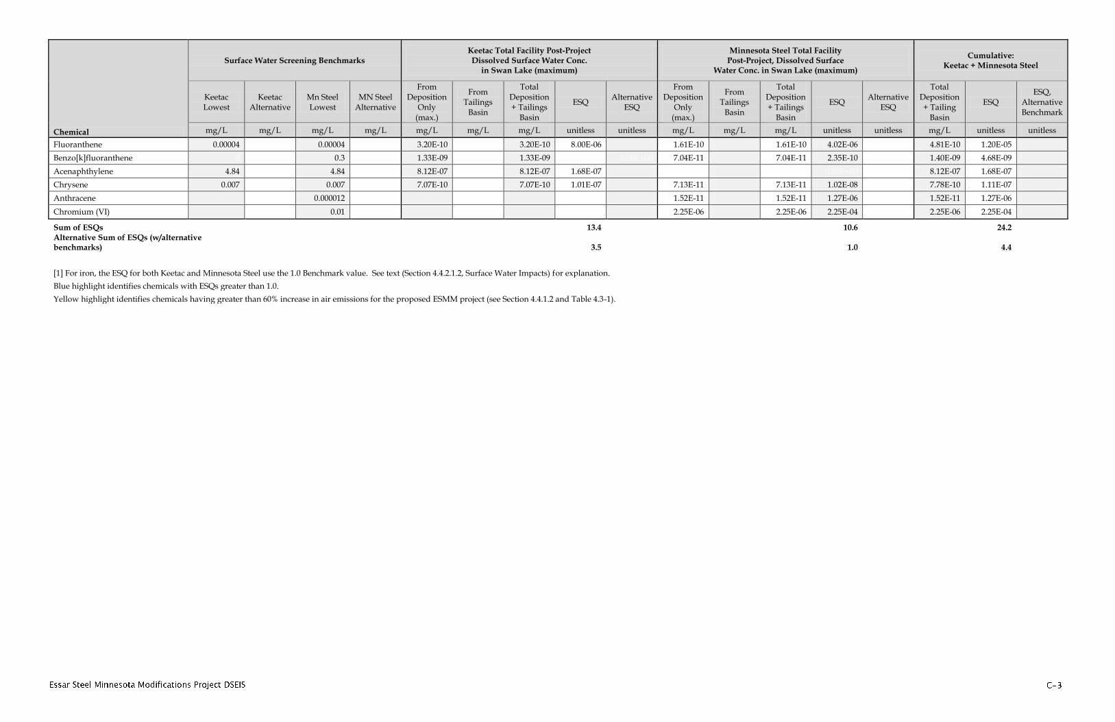
Sum of ESQs 13.4 10.6 24.2 Alternative Sum of ESQs (w/alternative benchmarks) 3.5 1.0 4.4

[1] For iron, the ESQ for both Keetac and Minnesota Steel use the 1.0 Benchmark value. See text (Section 4.4.2.1.2, Surface Water Impacts) for explanation.

Blue highlight identifies chemicals with ESQs greater than 1.0.

Yellow highlight identifies chemicals having greater than 60% increase in air emissions for the proposed ESMM project (see Section 4.4.1.2 and Table 4.3-1).

Appendix D. Supplemental Risk Assessment Information

This appendix presents assessments of a more technical nature identified by preparers of the SEIS during the review of supporting texts pertaining to the ecological risk assessment (Chapter 4.4) and cumulative mercury deposition (Chapter 5.3). The chapters contain references to this text where appropriate.

This subsection presents additional toxicological assessments that were conducted to support the screening level assessment of ecological risk in Chapter 4.4 of the SEIS. The additional assessment is focused on three specific parts of the ecological risk assessment: food web bioaccumulation, basis for alternative TRVs, and assessment of cumulative risk to Swan Lake from combined impacts from the proposed ESMM project and the Keetac project.

The TRVs for surface water, soil and sediment address toxicity to organisms that have direct contact with a chemical. Few of the standards specifically address the potential for chemicals to bioaccumulate in the food web. For example, water quality standards do not consider the extent to which mercury can accumulate in fish and subsequently be available to eagles at much higher concentrations than they might otherwise be exposed to through direct contact with surface, soil or sediment. The ingestion of terrestrial invertebrates by small birds, which have high consumption rates per body weight, also tends to be sensitive to exposure via the food web. Therefore, certain chemicals known as persistent, bioaccumulative and toxic (PBT) cannot be fully assessed using screening level TRVs (MNDNR, 2010; Ohio EPA, 2003, p. 3-7).

A list of chemicals considered to be PBT and a priority concern are listed by the EPA.1 As pertains to this site, it includes several PAHs, PCBs, cadmium, lead, and mercury. A longer list of PBT chemicals applicable to this site might be identified if TRV criteria provided by the Ohio EPA were used, which is inclusive of any chemical having a Kow (Octanol-Water partition coefficient; used to estimate the potential for a chemical to accumulate in fatty tissues) greater than or equal to 3.0 and that are not otherwise metabolized. For example, ecological risk assessment guidance provided by the State of Texas also identifies chromium, copper, nickel, selenium, thallium, zinc, and dioxin as bioaccumulative chemicals, among others not specifically identified as COPIs for this site.2

Some food web bioaccumulation concerns for select chemicals in soil are addressed by the TRVs available through The Risk Information System. The soil TRVs for cadmium and lead that are provided by the Eco-SSLs specific for birds and mammals do consider a default food ingestion pathway. In 2007, similar TRVs were published for manganese, nickel, selenium, zinc, and PAHs.3 Preparers of this SEIS reviewed these publications and determined that the new information would not result in selection of lower TRVs for this risk assessment. Work on TRVs that consider food web exposure for PCBs in soil has not been conducted.

The potential for mercury to bioaccumulate in fish tissue is assessed (Barr, 2006a); however, the risk implication of increased fish tissue concentrations to fish consuming organisms is not assessed. MPCA’s (2006) screening spreadsheet model was used to provide a conservative estimate of potential fish tissue concentration changes due to the project’s potential mercury emissions. Included in the MPCA’s screening spreadsheet

1 See http://www.scorecard.org/chemical-groups/one-list.tcl?short_list_name=pbt. 2See http://www.tceq.state.tx.us/assets/public/remediation/eco/0106eragupdate.pdf. 3 A current list of available documents is available at http://www.epa.gov/ecotox/ecossl/. Note that not all documents listed provide criteria for food web pathways.

http://www.scorecard.org/chemical-groups/one-list.tcl?short_list_name=pbt

http://www.tceq.state.tx.us/assets/public/remediation/eco/0106eragupdate.pdf

http://www.epa.gov/ecotox/ecossl/

model is a calculation that provides an estimate of the potential increase in fish tissue mercury concentration associated with an upper 95% confidence limit of the facility’s predicted mercury emissions. The results of the screening mercury deposition analysis estimate a maximum potential increase in fish mercury concentration of approximately 0.006 – 0.009 parts per million (ppm) in each of the three lakes studied. Existing upper 95% confidence limit fish tissue concentrations are 0.51 ppm for Big Sucker Lake, 0.70 ppm for Snowball Lake, and 0.42 ppm for Swan Lake.

The results of the mercury modeling suggest that there are other sources of mercury to which fish are exposed to, and that the relative contribution from the original MSI project is quite small. As described elsewhere in this SEIS, activated carbon treatment on the indurating furnace is included in the proposed ESMM project that would reduce mercury emissions from this source by 80%. This would further reduce mercury impacts on fish tissue concentration.

While water quality and fish tissue impacts are predicted to be low, the mercury assessment does not fully address risk assessment needs because neither the existing nor increased levels of mercury in fish tissue are assessed in terms of potential toxicity to organisms that would ingest the fish. Moreover, while mercury provides a good estimate of overall concern for PBT issues, the results do not exclude the potential for risks from other chemicals. For example, predicted concentrations of cadmium and lead in air, soil and water at location 7 (Figure 4.4-1) are both higher than that predicted for mercuric chloride or methyl mercury. A comprehensive assessment of bioaccumulation and food web exposure would need to consider concentrations of each PBT chemical in the environment, exposure via all environmental media (sediment, soil and surface water), bioaccumulation potential, and toxicity. The Ohio EPA (2003) provides one approach for doing so.

Iron is the principal chemical of potential concern for surface water along the southern boundary of the mine site. The lowest reported TRV in The Risk Information System is 0.01 mg/L based on an EC204 for daphnids. The possible use of the EC20 value was identified in a summary table but was not discussed as a possible TRV in the SLERA for the original MSI project (Barr, 2006). Rather, discussion focused on the applicability of the U.S. National Ambient Water Quality Criteria value of 1.0 mg/L. This nationally recommended criterion is based on a number of laboratory and field studies indicating lethal toxicity to fish and macroinvertebrates at concentrations near 1.0 mg/L. Accordingly, it is a more robust value for a TRV than the 0.01 value that is derived from a single study.

In a critique of the National Ambient Water Quality Criteria value, Barr (2006) points out that the criterion is based on 30-year old studies that lack all of the documentation needed to consider them as high quality by contemporary standards. Moreover, the solubility and bioavailability of iron in natural environments is widely influenced by many factors, often causing iron to precipitate and settle as sediment before reaching toxic levels in the water. However, the sediments formed from the precipitate can also be toxic at adequately high iron levels. Barr identifies a newer study demonstrating that iron concentrations below 40 mg/L had no severe effect on the survival of the

4 EC20 refers to a concentration at which 20 percent of the organisms exhibit a toxic effect. The effect may include reproductive effects or other adverse effects including death.

mayflies during a 30 days test exposure, and applies the 40 mg/L value as an alternate TRV.

The available data indicate that iron toxicity can range widely in natural environments. While based on older data, the U.S. National Ambient Water Quality Criteria remains a widely used value that ranks high on most hierarchies for selecting TRVs. For example, iron is currently regulated for the surface water discharge points for the mine pit maintenance dewatering from Pit 5 and Draper/Pit 6 locations to the Sullivan and Ann pits. The iron limit in the permit for these locations is 1.0 mg/L average and 2.0 mg/L maximum.

The National Ambient Water Quality Criteria for iron is based, among other considerations, on a number of observed cases where concentrations above approximately 1 mg/L have shown toxicity to fish and invertebrates in laboratory and natural settings (MNDNR, 2010). The selection of a single study using a single species as a basis for a TRV without thorough reexamination of all new information is not consistent with typical screening level risk assessment practice, particularly since the proposed TRV is 40 times greater than the National Ambient Water Quality Criteria. However, it does provide a measure of the range of uncertainty associated with interpreting risks from iron exposure.

An ESQ of 10.9 is derived when using a TRV of 1.0 mg/L, while the ESQ reduces to 0.3 when the alternative TRV of 40 mg/L proposed by Barr is used. Applying the BLM interpretive criteria to these ESQs indicates risks in the range of moderate (or borderline high) to low. The predicted concentrations are the incremental increase over existing background levels that would be due to future mining. Existing background levels of iron may increase the potential for adverse effects. Efforts to reduce uncertainty about potential iron toxicity to aquatic resources would need to further evaluate or measure the complex geochemistry of iron in areas of potential concern. Efforts would also need to consider the degree to which the aquatic ecosystem in the area is naturally adapted to the iron enriched geology of the region.

The lowest TRV for magnesium is 0.647 mg/L, which produces an ESQ of 1.3. While technically greater than the 1.0 decision criteria, estimates of risk are generally considered accurate to only one significant figure, which means that the ESQ of 1.3 is not meaningfully different from 1.0. Moreover, there is considerable uncertainty about magnesium toxicity.

The TRV is listed in The Risk Information System as an EPA Region 6 surface water screening benchmark; however, efforts by MNDNR to verify this information could not confirm this value. Barr (2006) indicates that the TRV is established by the Texas Natural Resource Conservation Commission and based on a hardness of 50 mg/L. However, a review of this information identified a chronic freshwater criterion of 3.2 mg/L that is not hardness dependent but based on wastewater permitting needs in Texas.5 Moreover, Suter and Tsao (1996) indicate that the chronic value derived from a study using daphnids is below commonly occurring ambient concentrations of this nutrient chemical; therefore, it was deemed inappropriate to establish a standard. While the document is unclear, this comment appears to be in reference to a TRV of 82 mg/L, the alternative TRV used by Barr (2006). Barr (2006) also notes that the background concentration of magnesium in Swan Lake is approximately 17.5

5 See http://www.tceq.state.tx.us/assets/public/remediation/eco/0106eragupdate.pdf, footnote b, page 18.

http://www.tceq.state.tx.us/assets/public/remediation/eco/0106eragupdate.pdf

mg/L. Presumably this is a natural background concentration and not a response to historic mining operations.

Toxicological data to support a TRV is extremely limited. When a TRV is less than naturally occurring background concentrations, background concentrations are an appropriate screening level benchmark for assessing potential risk.

Available data permits an assessment of the potential for the proposed ESMM project to increase background concentrations of magnesium. Tailings related influences on Swan Lake estimated for the original MSI project were predicted to increase magnesium concentrations by 5.14 mg/L. This amount of influence is greatly reduced for the proposed ESMM project to 0.822 mg/L due to revised groundwater flow estimates (see Section 4.4.1.2). Potential influences from air emissions were estimated based on similarity to calcium and determined to be insignificant (Barr, 2010). The proposed ESMM project is not predicted to substantially increase magnesium levels above reported background concentrations. Accordingly, risks for magnesium exposure are considered to be low.

The only TRV provided for phosphorus in The Risk Information System is a value of 0.0001 mg/L, obtained from EPA Region 6. Using this value produced an ESQ greater than 1.0. However, this TRV is only applicable to salt water (Barr, 2006).6 Accordingly, The Risk Information System is of no use, and an alternative basis for assessing phosphorus is necessary.

The State of Minnesota provides water quality standards for phosphorus for Class II waters that are intended for aquatic life and recreation uses. Phosphorus is a nutrient that can cause eutrophication and algal bloom. A value of 0.030 is identified for the Northern Lakes and Forest Ecoregion, a value only slightly higher than natural background for the area but below the current concentration in Swan Lake.

A study of nutrients in Swan Lake indicates that the current background concentration of phosphorus in Swan Lake is about 0.008 mg/L (Wenck Associates, Inc. 2006), while in 1986 Swan Lake’s phosphorus concentration was 0.022 mg/L. The median for the Northern Lakes and Forest Ecoregion was identified to be 0.023 mg/L. This information suggests that phosphorus concentrations are decreasing over time and remain below state standards. Refer to Section 4.1.1.2 for more details on background water quality and nutrient trends in Swan Lake.

Available data permit an assessment of mining related contributions to the observed increase in phosphorus concentrations. Barr (2006) estimated that contribution of phosphorus from the tailings basin discharge and seeps to Swan Lake from the original MSI project to be 0.0007 mg/L. This influence would be reduced by the reduced seepage and the elimination of the discharge for the proposed ESMM project. Air emission influences to Swan Lake were approximated by Barr (2010) based on similarities to calcium and were determined to be relatively minor. The available information indicates that the proposed ESMM project will not result in increased phosphorus concentrations that exceed state standards or degrade designated beneficial uses.

6 See also http://www.tceq.state.tx.us/assets/public/remediation/trrp/swrbelstable.pdf, p. 4.

http://www.tceq.state.tx.us/assets/public/remediation/trrp/swrbelstable.pdf

Appendix C presents the results of the cumulative risk assessment conducted by Barr (2010). No updates or revisions were made by Barr to the table to reflect increased air emissions associated with the proposed ESMM project or decreased groundwater seepage related to the tailings impoundment. The calculations were not revised because Barr considered air emissions to be not significant relative to other influences. Also, cumulative risk estimates are interpreted by Barr to be low, precluding the need for more detailed assessment.

Aluminum, iron and manganese were identified for the original MSI project to be the only chemicals derived from air emissions that contributed a notable amount to the total estimated dissolved water concentration in Swan Lake (Barr, 2006; Barr, 2010). While Appendix C was completed prior to completing the emission inventory for the proposed ESSM project, the conclusions to be derived from Appendix C are not substantially affected by the revised emission rates (Barr, 2011; Table 4.1-1). However, a small amount of uncertainty exists in this conclusion for fluoride (and hydrogen fluoride), potassium, and thallium as indicated by the yellow highlighting in Appendix C. Emissions for these chemicals are predicted to increase by more than 60% (Table 4.1-1), yet no quantitative information is provided in the cumulative assessment. Accordingly, all other predicted chemical concentrations in Swan Lake as a result of the proposed ESMM project are estimated to be 16% of those for the original MSI project. This reduction reflects a reduced groundwater seepage related impact (see Chapter 4.1 and Section 4.4.1.3).

Several chemicals were only assessed for one facility, and could therefore not be assessed for cumulative impacts. For a few chemicals, the ESQs derived for only Keetac emissions are high enough to suggest that the ESQ might exceed 1.0 if relatively higher contributions derive from the proposed ESSM project. Fluoride has an ESQ of 0.8 from Keetac emissions but is not included in the MSI part of the results. Elemental mercury has a fairly low ESQ from Keetac emissions (0.07), but high enough to potentially cause a cumulative ESQ to exceed 1.0 depending on the MSI concentration. Dioxin (which is listed in Appendix C as TCDD, 2, 3, 7, 8-) has an ESQ of 0.03. Dioxin concentrations predicted in Snowball Lake were 5.13E-11 mg/L in a prior Barr report (Barr, 2006b). Even when adjusted upward by 60% to reflect increased emissions for the proposed ESMM project, the cumulative ESQ would remain substantially below 1.0. The Keetac ESQs are far below 1.0 for all other chemicals not evaluated for the original MSI project. Moreover, for most chemicals evaluated for both facilities, the Keetac facility is predicted to contribute higher concentrations than the original MSI project. Accordingly, it is unlikely that additional assessment of MSI emissions not currently reported would lead to different conclusions about cumulative risk. Fluoride is a possible exception, due to the large increase in hydrogen fluoride and fluorine/fluoride emissions identified in the human health risk assessment.

The results of the cumulative assessment indicate varied sources of influence to Swan Lake water quality for chemicals contributing at least 0.1 to the ESQ. The total ESQ for all chemicals from both facilities ranges from 24.2 for the lowest TRV to 4.4 when using an alternative TRV. These totals suggest an overall high to moderate level of risk when applying the BLM interpretative criteria defined in Section 4.4.2.2 of the SEIS. However, risks from exposure to multiple chemicals are not likely to be additive, particularly where risk to different species or different kinds of toxic effects are represented by the chemical-specific TRVs. However, for chemicals with an ESQ greater than 1.0, a more detailed assessment

of the findings is presented to support a qualitative assessment of the uncertainty associated with the quantitative risk estimates. .

Cumulative ESQs greater than 1.0 are reported for boron, copper and magnesium. Each chemical is assessed individually. The human health risk assessment (Barr, 2011) identified a 17 percent decrease in boron emissions, a 1 percent increase in copper emissions, and a 20 decrease in magnesium emissions for the proposed ESMM project versus the original MSI project. These deviations are not applied to the quantitative risk estimates presented below. Emission deviations of this magnitude do not change the overall content or conclusions of the text for these three chemicals.

Cumulative ESQs for boron range from 5.5 to 0.29, depending on the choice of TRV. Using the lowest TRV, the ESQ is 3.9 for Keetac and 1.5 for MSI. Under conditions for the proposed ESMM project (higher air emission and lower water related emissions), influences to Swan Lake are about ten times higher for water related emissions.

For Boron in surface water, the lowest TRV is 0.0016 mg/L. This value is used by EPA Region 6 as a surface water screening benchmark. The value is derived from a widely applied reference publication by Suter and Tsao (1996). This document states that the standard is based on an EC20 value obtained from a 21-day test on Daphnia magna conducted in1984, while noting that another 21-day test of Daphnia magna by Lewis and Valentine conducted in 1981 provided the lowest daphnid chronic value. Daphnia magna is a type of aquatic invertebrate. EC20 means the highest tested concentration causing less than 20% reduction in the product of growth, fecundity (reproductive capacity), and survivorship in a chronic test with a daphnid species. These benchmarks are intended to be indices of population production. Derived in this manner, the TRV is called a Tier II Secondary Chronic Value, which means that it is recognized as being derived from a limited amount of toxicological data.

Barr (2010) references several studies based on various aquatic species that demonstrate much less toxicity, with some species tolerating up to 10 mg/L. They select Minnesota’s industrial use water quality standard of 0.5 mg/L as an alternative to the 0.0016 mg/L used by EPA Region 6. This standard is applicable for agricultural uses like livestock watering. Industrial use standards are generally higher than standards for other kinds of water uses. Accordingly, an industrial use standard is not the most desirable basis for assessing risk.

It is customary for TRVs to default to local, natural background levels when background levels exceed risk-based TRVs. Barr also indicates that the background water quality in Swan Lake is 0.002 mg/L (MNDNR, 2010), which is very nearly the same value as the 0.0016 mg/L TRV. The incremental increase above background from Keetac is predicted to be 0.006 mg/L, or about three times the background concentration.

The toxicity of Boron appears to vary widely among species and under different water quality conditions. Available data suggests that some species may be adversely affected at the concentrations predicted. On-site monitoring of biota would be necessary to reduce uncertainty.

Cumulative ESQs for copper range from 1.5 to 0.17, depending on the choice of TRV. Only 0.07% of the cumulative ESQ is associated with the proposed ESMM project when the results are adjusted to reflect reduced water related emissions.

The lowest available TRV is 0.00023 mg/L based on lowest chronic value for a test using Daphnids. This methodology tends to produce TRVs that are lower than National Ambient Water Quality Criteria, which consider a broader range of test results, natural background concentrations, and a general objective of protecting most species most of the time. Barr utilizes the Canadian Water Quality Criteria of 0.002 mg/L, which is somewhat lower than the U.S. National Ambient Water Quality Criteria of 0.009 mg/L that is provided in The Risk Information System. These criteria are hardness dependent, which means that the criteria increase with increasing levels of hardness for the specific water body that the standard is applied to. Barr (2006) indicates that MNDNR classifies Swan Lake as a “hard-water walleye lake.” This suggests that a higher TRV may be appropriate; however, a site-specific TRV based on local hardness concentration was not developed for this project.

The selection of an alternative TRV for copper applies a generally accepted hierarchy. This supports emphasis on the alternative ESQ in interpreting risk. However, National Ambient Water Quality Criteria does not ensure protection of all species all the time and available data suggests that some species may be impacted at lower levels.

A 2007 update to the National Ambient Water Quality Criteria for copper establishes the use of the Biotic Ligand Model for developing TRVs for copper. This model uses the following site-specific water quality data to calculate a freshwater copper criterion: temperature, pH, dissolved organic carbon (DOC), calcium, magnesium, sodium, potassium, sulfate, chloride, and alkalinity.7 While performing such a detailed calculation may be beyond the level of effort appropriate for a screening level assessment, it is instructive to know that this more detailed basis for assessing copper toxicity exists if future conditions warrant.

Cumulative ESQs for magnesium range from 13.2 to 0.1, depending on the choice of TRV. About 24% of the cumulative ESQ is associated with the proposed ESMM project when the results are adjusted to reflect reduced water related emissions.

The uncertainty associated with assessing toxicity from magnesium exposure is described above for Swan Lake. As previously stated, the background magnesium concentration in Swan Lake is reported to be 17.5 mg/L. Keetac is predicted to increase concentrations by about 3 mg/L (per Appendix C), while the proposed ESMM project is predicted to add about 1 mg/L (per Table 4.4-2). While limited available toxicology data suggest that this increase and the total concentration might be toxic to some populations of organisms, the potential effects to Swan Lake are uncertain but likely limited. Background concentrations of magnesium may support species with more tolerance to magnesium.

7 See http://water.epa.gov/scitech/swguidance/waterquality/standards/criteria/aqlife/pollutants/copper/fs-2007.cfm.

http://water.epa.gov/scitech/swguidance/waterquality/standards/criteria/aqlife/pollutants/copper/fs-2007.cfm

http://water.epa.gov/scitech/swguidance/waterquality/standards/criteria/aqlife/pollutants/copper/fs-2007.cfm

This subsection presents additional assessment of statistical methods used to assess mercury deposition and bioaccumulation in fish presented in Chapter 5.3 of the SEIS.

As described in Chapter 4.4, the MPCA had developed the MMREM methodology for assessing the incremental increase in mercury concentrations in fish that would result from increases in mercury concentrations in air (see Chapter 5.3). The average mercury fish tissue concentration in a lake is an important input into this assessment. The assessment uses measured background concentrations of mercury in fish tissue from a number of lakes that are routinely monitored by the MPCA. How this fish tissue data is statistically analyzed can affect the predicted outputs of the MMREM assessment. For a given ambient air concentration of mercury, a larger determination of a background fish tissue concentration will result in a larger incremental increase in fish tissue concentration and a larger incremental increase in the hazard quotient. Three issues were identified that influence the background fish tissue concentration observed for this project.

ProUCL software developed by EPA was used to test the distribution and to calculate the 95 percent UCL of the mean fish tissue concentration for each data set. Barr used an outlier test method within the ProUCL software to identify measurements that were outside the expected distribution of measurement results at a 95 percent level of confidence. This approach resulted in excluding the two highest measurements for the Nashwauk area lakes (representing 4 fish averaging 27.6 inches in one case and two fish averaging 25.5 inches in another case), one highest measurement for Oxhide Lake (representing one fish averaging 26 inches), and one highest measurement for Snowball Lake (representing four fish averaging 27.6 inches). MPCA disagrees with this approach, which has the net effect of reducing the predicted increase in mercury levels in fish tissue concentrations that are attributed to the project. Statistical outlier tests serve as an aid for identifying data that might have issues such as measurement errors. However, there is no information indicating that these data points should be discarded from the assessment. Conversely, the fact that these measurements are for larger, older fish that have a greater potential to accumulate mercury over longer period of time suggests that they should be retained in the assessment as valid. The degree to which the approach used underestimates future fish tissue concentrations is dependent upon the magnitude of the outlier, the number of fish represented by the outlier, the total number of fish data available for a lake, and the magnitude of the project-related mercury concentration in air. Accordingly, it is not possible to accurately judge the degree to which fish tissue concentrations are underestimated.

Another element of uncertainty in the approach used to statistically evaluate fish tissue concentrations concerns options for considering composited samples. The statistical methods used to determine averages assume that each data point is independent and of equal weight to other data points. When fish tissue from multiple fish are blended and used to analyze a single fish tissue concentration, the resulting data point carries more “weight” than a sample from a single fish. Barr did not assess the potential implications of this issue. This leaves some uncertainty about the reported 95th upper confidence limit of the mean concentration. The degree of uncertainty can be roughly approximated by considering the difference between the absolute mean and the 95th UCL of the mean, which provides a sense of the amount of variability in the data. The absolute mean difference was never greater than 0.1 mg/kg for any lake, while the calculated 95th UCL values ranged from 0.3 to 0.59 mg/kg across the different lakes studied.

Finally, Barr used all data available as of 1980, which is consistent with MPCA guidance (2006a) when there are a limited number of data points for a lake. However, MPCA

guidance indicates that only data collected in the past 10 years should be used where adequate data exist. 114 data points were available for the Nashwauk area lakes. The extent to which bioaccumulation rates have changed over the years was not assessed and is otherwise difficult to discern from a visual inspection of the data as presented. It is unknown to what extent current estimates of average mercury fish tissue concentrations are biased by older data.

Barr, 2011. Supplemental Human Health Screening-Level Risk Analysis, Version 1. Prepared for Minnesota Steel Industries, LLC. January, 2011.

Barr, 2006. Screening-Level Ecological Risk Assessment for Chemicals Potentially Emitted to Air and Their Estimated Deposition to Nearby Receptors. Prepared for Minnesota Steel Industries, LLC. August 2006.

Barr, 2010. Response to Ecological Data Submittal Comments Dated October 14, 2010, Technical Memorandum to Bill Johnson, MNDNR and Lisa Fay, MNDNR, November 2.

Minnesota Department of Natural Resources (MNDNR), 2010. Comments, Response to Comments, and Final Clarifications and Path Forward regarding the July 14, 2010 Technical Memorandum from Cliff Twaroski, Barr Engineering Company, regarding the Essar Steel Expansion project, October 14.

Minnesota Pollution Control Agency (MPCA), 2006. MPCA Mercury Risk Estimation Method (MMREM) for the Fish Consumption Pathway (Local Impacts Assessment), Version 1.0, http://www.pca.state.mn.us/publications/aq9-16.pdf, December 2006.

Ohio EPA, 2003. Guidance for Conducting RCRA Ecological Risk Assessments. March 2003. State of Ohio, Environmental Protection Agency, Division of Hazardous Waste Management, Columbus Ohio 43216.

Suter, G. & Tsao, C., 1996. Toxicological Benchmarks for Screening Potential Contaminants of Concern for Effects on Aquatic Biota: 1996 Revision, Prepared for the U.S. Department of Energy Office of Environmental Management, ES/ER/TM-96/R2, June.

Wenck Associates, Inc. 2006. Swan Lake Nutrient Study (31-0067), Itasca County, Minnesota. Prepared for Minnesota Department of Natural Resources in Cooperation with Minnesota Pollution Control Agency and for Minnesota Steel Industries, LLC.

essar steel minnesota modifications project - draft supplemental

Documents