error rate and statistical power of distance-based...
TRANSCRIPT
Error rate and statistical power of distance-based measures of phylogeny-trait
association.
Joe Parker1,2 and Oliver G. Pybus2
1. Kitson Consulting, Bristol, UK; Present address: School of Biological and Chemical Sciences,
Queen Mary, University of London, UK
2. Department of Zoology, University of Oxford, UK.
Running title: Performance of phylogeny-trait association statistics
Word count: xxxx 7,621
Corresponding Author:Joe ParkerKitson Consulting Limited60 Coleman RoadCamberwellLondon, SE5 7TGTel. +44 20-7703-8988Fax +44 [email protected]
1
1
2
3
4
5
6
7
8
9
10
11
121314151617181920

SUMMARY
Building on work presented previously (Parker et al., 2008), we study here a number of more
complex measures of phylogeny-trait association (, implemented in the program Befi-BaTS),
which take into account the branch lengths of a phylogenetic tree in addition to the
topographical relationship between taxa. Extensive simulation is performed to measure the
Type II error rate (statistical power) of these statistics including those introduced in Parker et al.
(2008), as well as the relationship between power and tree shape. The technique is applied to
an empirical hepatitis C virus data set presented by Sobesky et al. (2007); their original
conclusion that compartmentalization exists between viruses sampled from tumorous and non-
tumorous cirrhotic nodules and the plasma is upheld. The association index (AI), migration (PS),
phylodynamic diversity (PD) and unique fraction (UF) statistics offer the best combination of
Type I error and statistical power to investigate phylogeny-trait association in RNA virus data,
while the maximum monophyletic clade size (MC) and nearest taxon (NT) statistics suffer from
reduced power in some regions of tree space.
Keywords: BaTS, hepatitis C virus, Markov-chain Monte Carlo, Phylogeny-trait association,,
Markov-chain Monte Carlo, Phylogenetic uncertainty, simulation., hepatitis C virus, BaTS
2
1
2
3
4
5
6
7
8
9
10
11
12
13
14
15
16
17

IntroductionINTRODUCTION
Previously, we reviewed many areas of viral evolutionary biology where more accurate
estimation of the degree of association between the phylogenetic structure of a data set and the
distribution of trait values of some character of interest at the tips of that phylogeny is desirable
(Parker et al., 2008). These included viral phylogeography (Holmes, 2004; Starkman, 2003);
population structure (Carrington et al., 2005; Nakano et al., 2004); epidemiology (Leigh Brown
et al., 1997) and compartmentalization (Pillai et al., 2006; Salemi et al., 2005; Fulcher et al.,
2004) as well as T-cell escape (Bhattacharya et al., 2007; Komatsu et al., 2006; Sheridan et al,
2004).
However, we also noted that previously adopted methodologies such as AMOVA (Sullivan et al.,
2005), single tree estimation (Potter et al., 2004) or the Slatkin-Maddison test (Skatkin &
Maddison, 1989), were deficient in some respects; significantly they failed to correctly
incorporate phylogenetic error due to reliance on single-tree approaches to phylogeny-trait
correlation. As a result, these methods were unable to assign significance to observed
phylogeny-trait correlations. To address these concerns, Chapter Twoin Parker et al. (2008) we
presented a novel implementation (‘BaTS’) of three measures of phylogeny-trait association –
the Association Index (‘AI’; Wang et al, 2001); parsimony score (‘PS’; following Fitch, 1971b);
and introduced the new maximum monophyletic clade size statistic (‘MC’). BaTS calculates
these statistics in a Bayesian MCMC framework that takes into account phylogenetic uncertainty
by ‘averaging’ over the posterior distribution of trees. The Type I error rate of these statistics
was also measured through simulation and found to be correct.
In Chapter Four a large human immunodeficiency virus Type-1 (HIV-1) data set was
analyzed using BaTS to determine the evidence for genetic compartmentalization of viral
3
1
2
3
4
5
6
7
8
9
10
11
12
13
14
15
16
17
18
19
20
21
22
23
24
25
sequences (env & gag genes) in cervical tissue of 41 HIV-positive women. The
differences in the relative performance of the statistics on an empirical data set were
clear, with the AI and PS statistics appearing to be more statistically powerful than the
MC statistic. Overall, there was sufficient evidence from the BaTS phylogeny-trait
analysis to support the compartmentalization hypothesis; the single-tree approaches
employed in Chapter Four were statistically weaker.
The conclusions of Chapter TwoParker et al. (2008) form the starting point for this study. An
incorrect Type I error rate (false rejection of the null hypothesis) is generally taken to be a more
serious flaw in any statistical approach than a Type II error rate (failure to correctly reject the
null hypothesis where a significant result exists) since a definitive rejection of the null hypothesis
leads us to modify our model. However, in studies of viral evolution large amounts of sequence
data are often generated at considerable financial and scientific expense in order to investigate
a particular hypothesis (e.g., viral compartmentalization). In this light it seems clear that high
statistical power (low Type II error) is also desirable in a statistical test. Accordingly, this study
uses extensive simulations to quantify the Type II error rate of phylogeny-trait association
statistics, as implemented in a Bayesian framework.
The AI, PS and MC statistics investigated in Chapter Twopreviously depend only on tree
topology; they take into account only the branching order of taxa, not the absolute evolutionary
distance between them. However, RNA viruses are capable of very rapid evolution (Jenkins et
al., 2002; Drake et al., 1998) and their phylogenies exhibit a wide range of tree shapes, from
highly ‘comb’-like (internal nodes distributed towards the terminal taxa) in dengue virus, to stat-
like phylogenies with very long external branches (as in HIV population-level phylogenies) and
highly unbalanced trees (e.g. influenza virus A population phylogenies; Grenfell et al., 2004). It
4
1
2
3
4
5
6
7
8
9
10
11
12
13
14
15
16
17
18
19
20
21
22
23
24
25

is therefore reasonable to consider the relevance of branch length information to the estimation
of phylogeny-trait correlation.
Figure 1: Trees a) and b) have identical topologies. The association between the ‘red’ and
‘black’ traits and phylogeny, as measured by the AI statistic, is necessarily the same for both.
Figure 5.1 gives an example of two trees that differ in tree branch lengths but share a topology,
and have the same distribution of a hypothetical ‘red / blue’ trait at their terminal taxa. The AI
statistic introduced by Wang et al. (2001) here measures the strength of association between
the red or black traits’ distribution and the phylogeny (higher values reflect a stronger
association). Both the trees in Figure 5.1 would be calculated to have an AI of 0.059; this
suggests that the red / blue trait is equally correlated with phylogeny, and of equal biological
significance, in both data sets. However, the ‘red’ trait’s association with phylogeny has been
maintained through a considerable period of evolution and time in the clade containing taxa ‘e’
and ‘f’ in Figure 5.1b, while the same correlation has so far been maintained over a much
shorter period of evolution in Figure 5.1a. We might reasonably conclude that the association
pattern seen in Figure 5.1b is more significant than that seen in Figure 5.1a – yet because the
AI statistic ignores branch length information, we are unable to do so.
5
1
2
3
4
5
6
7
8
9
10
11
12
13
14
15
16
17
18

This chapter study investigates four new statistics that include branch length information as well
as taking into account the topological relationships among taxa. They are the phylogenetic
diversity (‘PD’) measure of Faith (1992); the Net Relatedness (‘NR’) and Nearest Taxa (‘NT’)
indices of Webb (2000; 2002); and the Unique Fraction (‘UniFrac’ or ‘UF’) statistic of Lozupone
& Knight (2005).
Figure 2: The trees presented in Figure 5.2; this time phylogeny-trait association is measured
by four statistics (UniFrac, Nearest Taxon (‘NT’), Net Relatedness (‘NR’) & Phylogenetic
Diversity (‘PD’)). The value of the statistic is proportional to the strength of association; higher
values are more strongly associated. Tree b) has stronger phylogeny-trait association than tree
a).
By including branch length information these statistics may be able to discriminate between the
two trees presented in Figure 5.1; Figure 5.2 shows the same phylogenies, but this time values
for the new statistics are given. This time tree b) shows a stronger phylogeny-trait association
than tree a) – the UniFrac, NT, NR and PD values are all higher.
6
1
2
3
4
5
6
7
8
9
10
11
12
13
14
15
16

This chapter study seeks to investigate, through extensive simulation, the Type I and Type II
error rates of all the statistics introduced in this chapter and those introduced in Chapter
TwoParker et al. (2008). The influence of tree shape on the Type I error rate is also
investigated: since this technique is implemented in a Bayesian framework, the observed and
null distributions of the association statistics are calculated from the posterior set of trees (PST).
This is sampled from the true posterior distribution of topologies (topologies are sampled in
proportion to their posterior probability) so power should be maintained equally well in
topologies that are traditionally problematic for evolutionary parameter estimation (e.g. star-like
trees). To illustrate the use of these statistics, weI apply them to an empirical data set of within-
patient HCV sequences, sampled from a number of different tissues by Sobesky et al. (2007).
WeI re-visit their central hypothesis of genetic compartmentalization between tumoral and non-
tumoral HCV-infected hepatocytes.
7
1
2
3
4
5
6
7
8
9
10
11
12
13

MethodsMETHODS
In this Chapter study weI add a number of new statistics to the BaTS package, first introduced
in the course of Chapter TwoParker et al. (2008). The new statistics differ from those
implemented previouslyin Chapter Two; they incorporate branch length information as well as
tree topology. Therefore it is more important in this Chapter to ensure the model of substitution
is correctly selected and estimated to obtain accurate estimates of genetic distance, in addition
to efficient sampling of the posterior distribution of tree topologies.
The Statistics:
In the foregoing descriptions, s is defined as a subset of taxa on phylogenetic tree that
only and exclusively possess a given discrete phenotypic trait value. They are not
assumed to be monophyletic.
Phylogenetic Diversity (‘PD’): The PD statistic was first proposed by Faith (1992) and is a
simple intuitive measure of the amount of ‘diversity’, or genetic distance, captured by a subset s
of taxa in a phylogeny. The PD of s here equals the sum of branch lengths (including terminal
branches) in the subtree connecting all taxa in s but excluding any branches (internal or
external) leading only to taxa that are not in s (the ‘minimum spanning path’, or MSP). To give
an estimate of the strength of phylogeny-trait association in a data set, the PDs of s is divided by
the sum of all branch lengths in the phylogeny. This measure is summed for all subsets in of
taxa present to give an estimate of the strength of association; in a completely-associated case
the MSP of each subset will be shorter (and PDs smaller) than in an interspersed case.
Nearest Taxon (NT): The NT score of s is defined as the sum, over all taxa in s, of branch
lengths between each taxon and the nearest taxon that is also in s. This definition is modified
8
1
2
3
4
5
6
7
8
9
10
11
12
13
14
15
16
17
18
19
20
21
22
23
24
25
from that proposed by Webb (2000) in two ways: Firstly, weI use branch lengths rather than
nodal distances. Secondly, and importantly, weI do not divide the sum of NT distances by the
maximum possible sum of nearest taxa distances in a tree to create an index. Instead, weI
simply measure the sum of NT distance for all taxa subsets in a tree. It is not necessary in the
context of this study to create an index as Webb (2000) originally did, since BaTS generates a
correct null distribution for the statistic through randomization of taxa trait allocations.
Furthermore, calculating the maximum possible value exactly is computationally expensive in
the current BaTS implementation, especially for large data sets.
Net Relatedness (NR): The net relatedness is defined as the sum of all pairwise distances
between all members of s. As with the NT statistic, Webb (2000) introduced the statistic using
nodal distances for calculation, and divided the NT by a maximum possible value of this statistic
for any equally-sized subset of taxa to create an index. Again, the statistic is implemented here
using estimated branch lengths in place of nodal distances and not as an index, instead
calculating the significance of the observed NR value by generating an appropriate null
distribution by simulation.
Unique Fraction (‘UniFrac’, or ‘UF’): This simple measure, introduced by Lozupone & Knight
(2005) is the proportion of internal branches on a phylogeny that connect nodes whose trait
values are unambiguously resolved following trait value reconstruction by parsimony (Fitch,
1971b). The sum of UF values for s is expressed as a ratio of the sum of internal branch lengths
of the tree.
9
1
2
3
4
5
6
7
8
9
10
11
12
13
14
15
16
17
18
19
20
21
22
23

Incorporating phylogenetic uncertainty
Phylogenetic uncertainty (statistical error in phylogenetic estimation arising from sequence data)
is taken into account using the approach developed in Chapter Two. The expanded computer
package, Befi-DIM-BaTS 0.1.1 Alpha (Distance Information Methods-Bayesian Tip-association
Significance) is available on requestfrom http://www.lonelyjoeparker.com/BaTS.
Simulation
PreviouslyIn Chapter Two, weI estimated the Type I statistical error (i.e. the probability of falsely
rejecting the null hypothesis) through simulation. If the statistic is correct then the distribution of
p-values of a set of randomly drawn phylogeny-trait associations should follow a unit uniform
distribution. Here, weI repeat that approach to investigate the Type I statistical error of the
newly-introduced PD, NT, NR & UF statistics.
In addition, weI conduct a new series of simulations to test the Type II error rate of all
phylogeny-trait association statistics. The Type II error rate is defined as the frequency at which
a method fails to reject the null hypothesis when it is false. This is also known as the ‘power’ of
a statistical method; a statistic may have a correct Type I error rate, but its applicability to
analysis will be limited if it is weak or overly conservative (of diminished power) since it may
ignore too many significant results.
High
(‘comb’)
10
1
2
3
4
5
6
7
8
9
10
11
12
13
14
15
16
17
18
19

Low
(‘star’)
Low B1
(‘symmetrical’)
High B1
(‘unbalanced’)
Figure 3: Diagram of the spread of tree shapes represented by the nine master topologies used
in simulation, ordered by their node spread ( statistic, vertical axis) and tree imbalance, (B1,
horizonal axis).
The set of test phylogenies simulated in Chapter TwoParker et al., (2008) were used to explore
the power of these statistics. Firstly, a set of test alignments were generated and analyzed in
BEAST to obtain a set of PSTs with which to test DIM-BaTSBefi-BaTS:
1. 1000 phylogenies were generated under a pure-birth process using Phylo-O-Gen
(available from http://evolve.zoo.ox.ac.uk). The tree imbalance (Colless, 1982) and node
spread (, Pybus & Harvey, 2000) statistics were calculated for each tree in the set. Nine
11
1
2
3
4
5
6
7
8
9
10
11
12

‘master’ topologies were selected that reflected all possible combinations of tree
imbalance and node spread for tree imbalance values of (0, 0.125, 0.5) and values of
(-2, 0, 2). Figure 5.3 shows a diagram of the range of tree shapes thus selected.
2. A large set (n = 1000) of alignments were simulated from each of the nine master tree
topologies by Seq-Gen (Rambaut & Grassly, 1997). Substitution model parameters
derived from typical human immunodeficiency virus Type 1 (HIV-1) data were used1.
Each alignment contained 32 taxa and was 300 nucleotides long.
3. The PST for each alignment was then estimated using BEAST v1.4 (Drummond &
Rambaut, 2007). An HKY85 + substitution model with codon-position-specific
substitution rates and the strict molecular clock enforced (rate fixed to = 0.017) under a
constant population-size demographic model.
4. The set of simulations was down-sampled (to n = 897) to reduce computation. The first
10% of each PST was removed as burn-in. The PSTs produced were used for the
shuffling procedure below.
5. Statistics that measure tree spread tree imbalance and node spread (two measures that
together, describe most aspects of tree topology) were calculated for these source trees
using code from the TreeStat program (Drummond & Rambaut, 2007. Available from:
http://tree.bio.ed.ac.uk); I developed a modified command-line interface to facilitate
batch processing (author’s work, available on request). The statistics calculated were:
B1 (Kirkpatrick & Slatkin, 1993); Tree-imbalance (Colless, 1982); Cherry count (Steel &
Mackenzie, 2001); and (Pybus & Harvey, 2000) and Fu & Li’s D (Fu & Li, 1993).
1 The substitution model parameters were derived from analysis of the env gene data set sampled
from Patient AB in BEAST analysis (Chapter Four). Transition : transversion ratio = 2.54;
Nucleotide frequencies, A=0.426, C=0.152, G=0.182; specific substitution rates for first, second
and third codon positions respectively, 1 = 0.0152, 1 = 0.0142, 1 = 0.0215 (in substitutions per
site per year).
12
1
2
3
4
5
6
7
8
9
10
11
12
13
14
15
16
17
18
19
20
21
22
1
2
3
4
5
In the second stage, the 897 PSTs generated in step 4 above were used to investigate the
power of the phylogeny-trait association statistics. In order to measure the Type II error rate it
was necessary to generate data sets with different levels of phylogeny-trait association as
follows:
1. Each taxon in each PST of the set of PSTs was initially labelled with a hypothetical
binary character trait (e.g., ‘black’ / ‘white’) using the known master topology (the
underlying ‘true’ tree) in step 1 above to ensure maximal phylogeny-trait association.
These phylogeny-trait labellings are referred to as ‘completely associated’.
2. A new set of phylogeny-trait associations were generated by selecting two taxa at
random and exchanging their trait values. This is referred to as a ‘shuffle’. Note that the
posterior set of trees remains unchanged; only the taxon-trait labelling is modified.
3. Re-arrangements were carried out to give multiple data-sets, each comprising 897 PSTs
with the same trees but varying numbers of shuffles. As the number of shuffles
increases, the tip-trait associations become more random, from the completely
associated set (0 shuffles) to a set with random taxon trait labels (10,000 shuffles). Data
sets of 1, 2, 3…33, 60, 70, 80, 90, 100, 500, 1000, 5000 & 10000 shuffles were
produced.
[4.] Each shuffled data set was analysed with DIM-BaTSBefi-BaTS (using 100 replicates to
calculate the null distribution) to determine: a) the frequency of positives in each statistic
(statistics whose observed values p ≤ 0.05) and b) the mean significance (p-value) of
each statistic. In addition, the cumulative density function (CDF) of each statistic for
every shuffled set was determined by ordering and binning the p-values obtained. These
CDFs were compared to a unit uniform distribution using the Kolmogorov-Smirnov test
(Lilliefors, 1969; Massey, 1951) to investigate the transition between the completely
associated, interspersed, and random cases of phylogeny-trait association.
13
1
2
3
4
5
6
7
8
9
10
11
12
13
14
15
16
17
18
19
20
21
22
23
24
25
26

Empirical Data
To illustrate the application of this technique to viral sequence data, weI analysed an empirical
hepatitis C virus (HCV) data set reported by Sobesky et al. (2007). The authors sought to
determine whether significant genetic compartmentalization existed between HCV virus
populations sampled from peripheral blood and from cirrhotic nodules (two normal and one
cancerous) of a post-transplant human liver. Individual hepatocytes were sampled by
microdissection whilst serum samples were taken in vivo. Data was collected from seven
patients and alignments spanned 573 nucleotides of the core gene.
To investigate the hypothesis of compartmentalization using the new methods introduced here,
a PST was calculated from the data (aligned using Se-Al; http://evolve.zoo.ox.ac.uk) using
BEAST 1.4 (Drummond & Rambaut, 2007) for two patients from the data set: P1 (n = 70
sequences) and P7 (n = 68 sequences). Substitution, clock and demographic models were
selected based on the most likely models identified for similar data (the core gene window of the
‘Anti-D’ within-patient data set in Chapter Three): a constant population-size model of
demographic growth and an HKY85 + model of nucleotide substitution with the strict
molecular clock enforced at 0.005 substitutions / site / year. Six MCMC analyses were
independently performed for 10,000,000 states each to check convergence. Taxa were labelled
with their tissue of origin, and analyzed in DIM-BaTSBefi-BaTS with 100 replicates used to
calculate the null distribution.
14
1
2
3
4
5
6
7
8
9
10
11
12
13
14
15
16
17
18
19
20
21
Results RESULTS
Type I Error rate
The number of significant results (p 0.05) obtained using each statistic when taxon trait labels
were shuffled 10,000 times is given in Table 5.1. This simulates random taxon trait allocation
(the null hypothesis), so equals the Type 1 error rate of these statistics. The CDFs of all
statistics were not significantly different from a unit uniform distribution in the 10,000 shuffles
data set.
Statistic Type I rate
AI 0.051
PS 0.046
UF 0.028
PD 0.041
NR 0.062
NT 0.041
MC 0.029
Table 1: Type I error rate of statistics implemented in the DIM-BaTS package. Error rate given
is the proportion of significant results (p 0.05) observed in a data set of 897 randomly
assigned tip trait values (binary character, 10,000 shuffles).
Type II Error rate
Figures 5.4 – 5.10 give the results for the AI, PS, PD, UF, NR, NT & MC statistics respectively.
In each figure, the top plot shows the cumulative density function (CDF) of the statistic for
15
1
2
3
4
5
6
7
8
9
10
11
12
13
14
15
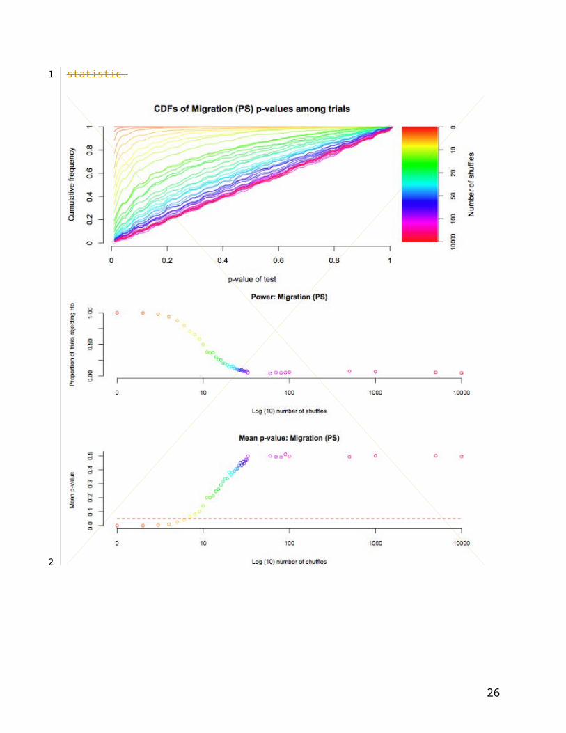
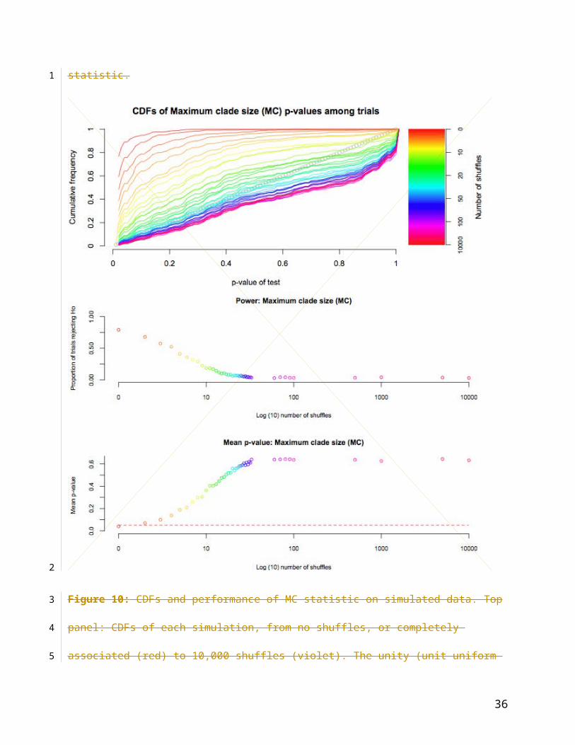
increasingly shuffled (more weak phylogeny-trait association) simulations, the centre plot shows
the proportion of rejections of H0 with increasing shuffles and the bottom plot shows the mean p-
value of the test with increasing shuffles. A red dashed line is drawn at p = 0.05.
CDF curves for most statistics show a smooth transition from maximal association (no shuffles)
to random tip-trait associations (approximately those simulations with more than 100 shuffles).
The randomly associated simulations have CDFs that are unit uniformly distributed (diagonal
grey line). However, the MC statistic CDFs quickly fall below the diagonal line, even at low
numbers of shuffles, indicating that the MC statistic is a weak measure. In contrast the NR
statistic CDF never reaches the diagonal line, suggesting the Type I error of this statistic may
not be correct at some levels of .
The Kolmogorov-Smirnov test (Lilliefors, 1969; Massey, 1951) was used to calculate the
significance of difference between p-values CDF of each simulation and a unit uniform
distribution (the expected distribution of p-values under the null hypothesis). The value of the
Kolmogorov-Smirnov statistic, D+, and significance, are given in Figure 5.11. Across the range
of shuffles used, the NR statistic showed the weakest departure from uniformity, while the NT
and PS statistics showed greatest departure from uniformity.
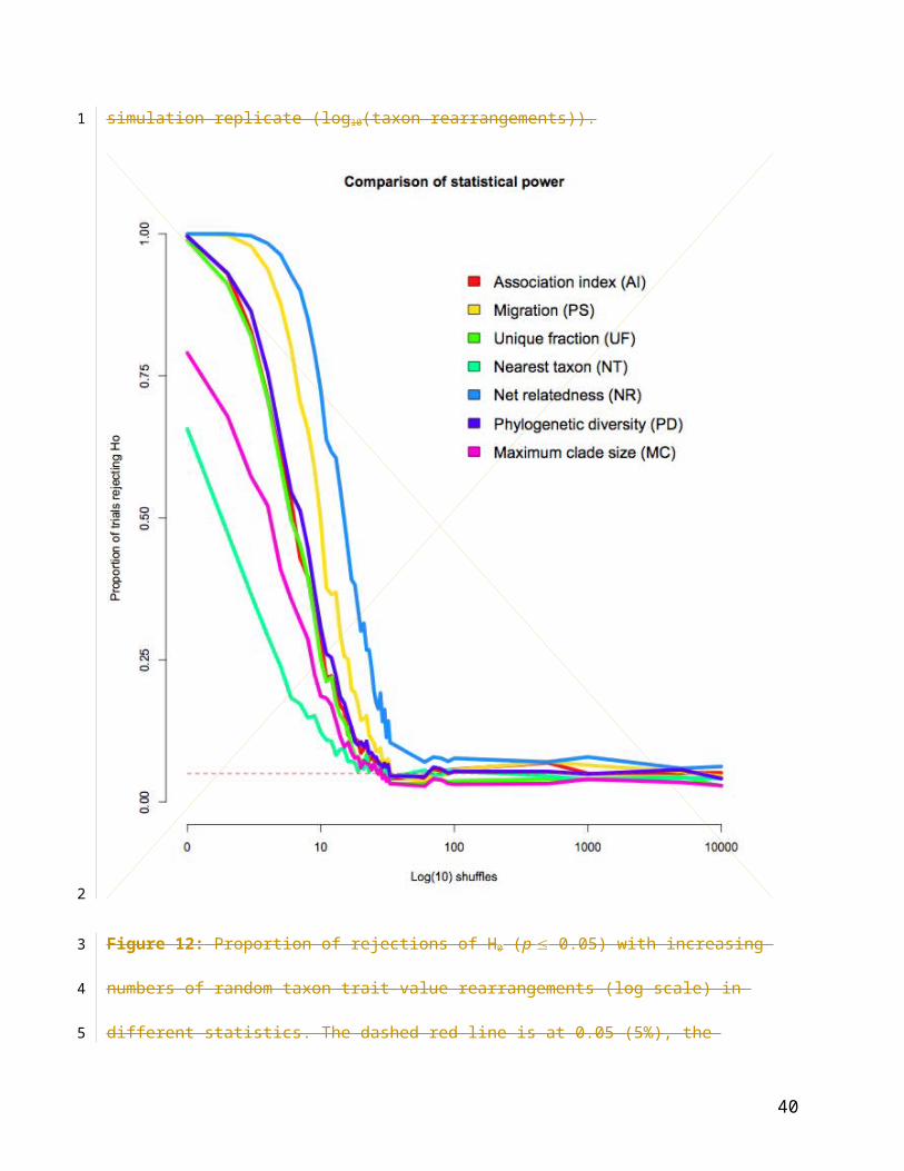
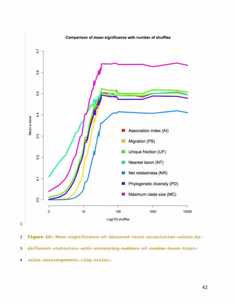
The number of significant tests and the mean significance of each test that are given in Figures
5.4 – 5.10 for each statistic are presented together for visual comparison in Figure 5.12 and
Figure 5.13. Figure 5.12 shows that the proportion of significant tests (p 0.05) obtained using
the MC and NT statistics declines more rapidly with the number of shuffles than other statistics,
indicative of weak statistical power. The PS and NR statistics, on the other hand, continue to
strongly reject H0 even in large numbers of shuffles. Equally, in Figure 5.13 the mean p-values
of the tests (probability of accepting the null hypothesis) rapidly increases with increasing
16
1
2
3
4
5
6
7
8
9
10
11
12
13
14
15
16
17
18
19
20
21
22
23
24
25
26

shuffles for the MC and NT statistics. In contrast, the PS and particularly, NR, statistics show a
lower mean significance.
17
1
2
3
4

Figure 4: CDFs and performance of AI statistic on simulated data. Top panel: CDFs of each
simulation, from no shuffles, or completely associated (red) to 10,000 shuffles (violet). The unity
(unit uniform distribution) is shown in grey. Centre panel: proportion of simulations rejecting H0
(out of 897 possible) with increasing trait re-arrangements (log10). Lower panel: mean
significance of observed AI statistic.
18
1
2
3
4
5
6
Figure 5: CDFs and performance of parsimony statistic (PS) on simulated data. Top panel:
CDFs of each simulation, from no shuffles, or completely associated (red) to 10,000 shuffles
(violet). The unity (unit uniform distribution) is shown in grey. Centre panel: proportion of
simulations rejecting H0 (out of 897 possible) with increasing trait re-arrangements (log10). Lower
panel: mean significance of observed parsimony statistic.
19
1
2
3
4
5
6

Figure 6: CDFs and performance of unique fraction (UniFrac) statistic on simulated data. Top
panel: CDFs of each simulation, from no shuffles, or completely associated (red) to 10,000
shuffles (violet). The unity (unit uniform distribution) is shown in grey. Centre panel: proportion
of simulations rejecting H0 (out of 897 possible) with increasing trait re-arrangements (log10).
Lower panel: mean significance of observed UniFrac statistic..
20
1
2
3
4
5
6

Figure 7: CDFs and performance of phylogenetic diversity (PD) statistic on simulated data. Top
panel: CDFs of each simulation, from no shuffles, or completely associated (red) to 10,000
shuffles (violet). The unity (unit uniform distribution) is shown in grey. Centre panel: proportion
of simulations rejecting H0 (out of 897 possible) with increasing trait re-arrangements (log10).
Lower panel: mean significance of observed PD statistic.
21
1
2
3
4
5

Figure 8: CDFs and performance of nearest taxon (NT) statistic on simulated data. Top panel:
CDFs of each simulation, from no shuffles, or completely associated (red) to 10,000 shuffles
(violet). The unity (unit uniform distribution) is shown in grey. Centre panel: proportion of
simulations rejecting H0 (out of 897 possible) with increasing trait re-arrangements (log10). Lower
panel: mean significance of observed NT statistic.
22
1
2
3
4
5
6

23
1
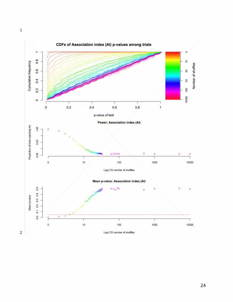
Figure 9: CDFs and performance of net relatedness (NR) statistic on simulated data. Top
panel: CDFs of each simulation, from no shuffles, or completely associated (red) to 10,000
shuffles (violet). The unity (unit uniform distribution) is shown in grey. Centre panel: proportion
of simulations rejecting H0 (out of 897 possible) with increasing trait re-arrangements (log10).
Lower panel: mean significance of observed NR statistic.
24
1
2
3
4
5
6

Figure 10: CDFs and performance of MC statistic on simulated data. Top panel: CDFs of each
simulation, from no shuffles, or completely associated (red) to 10,000 shuffles (violet). The unity
(unit uniform distribution) is shown in grey. Centre panel: proportion of simulations rejecting H0
(out of 897 possible) with increasing trait re-arrangements (log10). Lower panel: mean
significance of observed MC statistic.
25
1
2
3
4
5
26
1

Figure 11: The CDF for each statistic was compared to a unit uniform distribution under
increasing numbers of taxon rearrangements using a Kolmogorov-Smirnoff test. Shown are the
value of the difference statistic (lower plot) and p-value (upper plot) in each separate simulation
replicate (log10(taxon rearrangements)).
27
1
2
3
4
5

Figure 12: Proportion of rejections of H0 (p 0.05) with increasing numbers of random taxon
trait-value rearrangements (log scale) in different statistics. The dashed red line is at 0.05 (5%),
the proportion of trials expected to reject H0 under the null hypothesis at = 0.05 if the Type I
error rate is correct.
28
1
2
3
4

Figure 13: Mean significance of observed trait-association values by different statistics with
increasing numbers of random taxon trait-value rearrangements (log scale).
29
1
2
3

Sensitivity of phylogeny-trait association measures to tree shape
The distribution of common tree shape statistics on the set of PSTs used in each simulated data
set to test the phylogeny-trait association statistics (n = 897) is shown in Figure 5.14. The nine
topologies used to simulate the initial sequence alignments can be discerned as discrete
clusters.
Figure 14: Distribution of tree shape statistics of 897 simulated data sets used in this study.
Each alignment was simulated from one of nine master topologies picked to give a range of tree
topologies typical of human immunodeficiency virus (HIV) evolution. Simulated alignments were
analysed in BEAST version 1.4.6 (see Section 5.3.3 for details). Mean tree shape statistics
given were calculated from the posterior set of trees (PST) in each analysis using code from the
FigTree version 1.1 package (retrieved from http://beast-mcmc.googlecode.com; my
implementation is available on request).
30
1
2
3
4
5
6
7
8
9
10
11
12
13
14

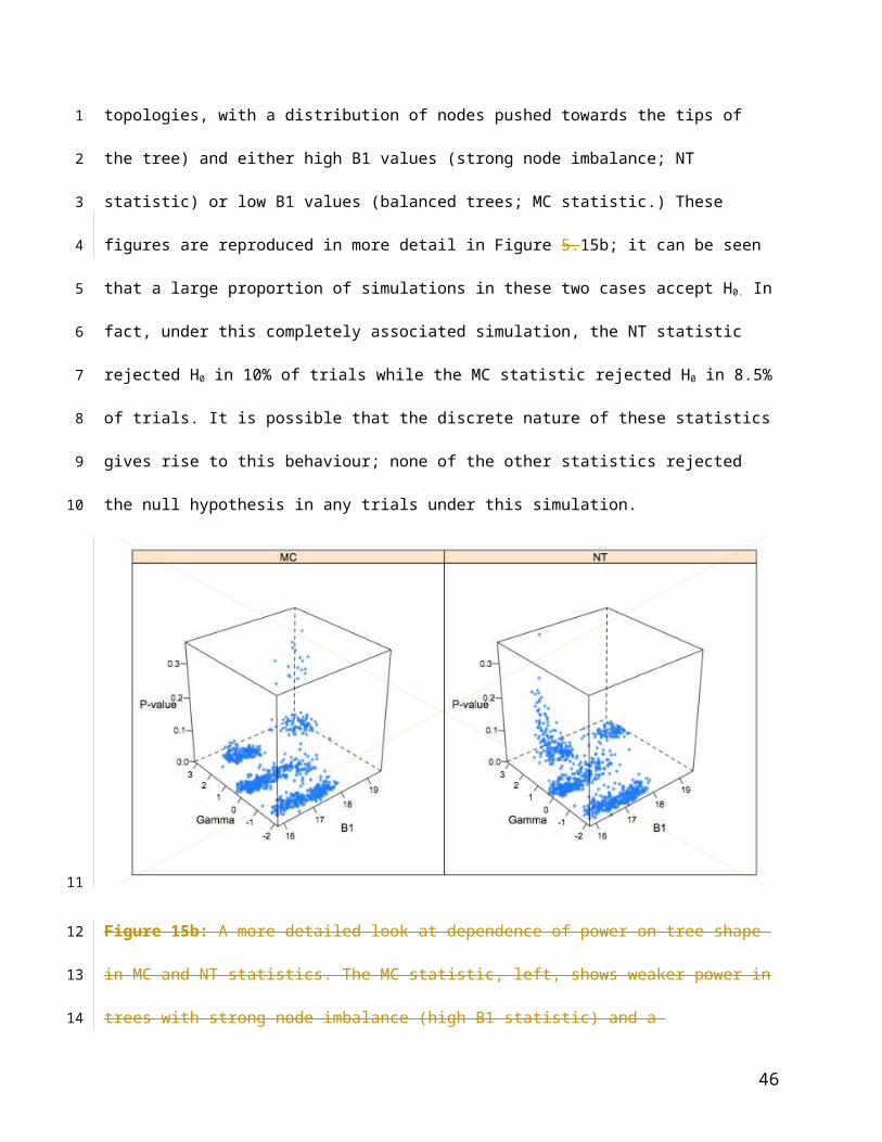
Figure 5.15a shows the distribution of p-values for each phylogeny-trait statistic when applied to
data sets with maximal phylogeny-trait association (i.e., no trait shuffles between tips). The
majority of statistics show no distinct pattern of failures to reject the null hypothesis (p > 0.05)
with tree shape, but the MC and NT statistics appear to do so at conditions of high values
(‘comb-like’ topologies, with a distribution of nodes pushed towards the tips of the tree) and
either high B1 values (strong node imbalance; NT statistic) or low B1 values (balanced trees;
MC statistic.) These figures are reproduced in more detail in Figure 5.15b; it can be seen that a
Figure 5.15a: Variation of statistical power with tree
shape for various phylogeny-trait association
statistics. Higher (Pybus & Harvey, 2000) values
indicate trees where the distribution of nodes is
skewed towards the tips of the phylogeny; Higher B1
values (Kirkpatrick & Slatkin, 1992) indicate greater
node imbalance. ‘P’, the significance of each data set
in the totally associated model.
31
1
2
3
4
5
6
7

large proportion of simulations in these two cases accept H0. In fact, under this completely
associated simulation, the NT statistic rejected H0 in 10% of trials while the MC statistic rejected
H0 in 8.5% of trials. It is possible that the discrete nature of these statistics gives rise to this
behaviour; none of the other statistics rejected the null hypothesis in any trials under this
simulation.
Figure 15b: A more detailed look at dependence of power on tree shape in MC and NT
statistics. The MC statistic, left, shows weaker power in trees with strong node imbalance (high
B1 statistic) and a distribution of nodes that is skewed towards the tips of the tree (high ). The
NT statistic, right, is also weaker in topologies with high , but in trees with evenly-balanced
nodes.
32
1
2
3
4
5
6
7
8
9
10
11
12

Compartmentalization in the liver during chronic HCV infection
Sobesky et al. (2007) studied compartmentalization between HCV viruses sampled from the
peripheral blood and two types of cirrhotic nodules (tumorous and non-tumorous) in seven
patients with chronic hepatitis C infection and hepatocellular carcinoma (HCC). 573nt
sequences were obtained from the core gene by clonal PCR; Patients P1 (n=70) and P7 (n=68)
from the original data set were re-analyzed in this study to examine the evidence for
compartmentalization with DIM-BaTSBefi-BaTS (see Section 5.3.4Methods). The DIM-
BaTSBefi-BaTS analysis identified significant compartmentalization by all methods (Table 5.2),
except in the MC measurements in Patient 1, where only clades of sequences sampled from
tumorous nodules were found to be significantly larger than expected due to chance. I also
measured the and B1 tree shape statistics in these patients with TreeStat (Table 5.2).
33
1
2
3
4
5
6
7
8
9
10
11
12

Patient 1
= -2.34, B1 = 35.5
Patient 7
= 3.20, B1 = 35.4
Statistic1
Mean
posterior
estimate
95 % HPD2
(lower,
upper) P3
Mean
posterio
r
estimate
95 % HPD2
(lower,
upper) P3
AI 2.83 2.07, 3.58 0.000 0.03 0.00, 0.09 <0.005
PS 29.72 25, 34 0.000 6.03 4, 8 <0.005
UniFrac 0.45 0.38, 0.52 0.010 0.85 0.77, 0.92 0.010
NT 442
373.16,
516.11 0.000 60.18
45.29,
76.86 <0.005
NR 17330
14185,
20894 0.090 2324 1758, 2984 <0.005
PD 1400 1193, 1631 0.000 290
226.12,
361.47 <0.005
MCN1 1.57 1, 2 0.080 9.96 10, 10 0.010
MCN2 2.09 2, 3 0.190 5.93 6, 6 0.010
MCserum 4.36 3, 6 0.270 31.33 31, 33 0.010
MCtumour 4.09 2, 7 0.010 10.85 6, 15 0.010
Table 2: Compartmentalization during hepatitis C virus (HCV) infection; data from Sobesky et
al., 2007. 1Statistics: AI, association index; PS, parsimony score; UF, unique fraction; NT,
nearest taxon; NR, net relatedness; PD, phylogenetic diversity; MC statistics, maximum
monophyletic clade sizes of: N1, first non-tumorous cirrhotic nodule; N2, second non-tumorous
cirrhotic nodule; serum, serum sample; tumour, tumorous cirrhotic nodule. 2Estimated upper and
34
1
2
3
4
5

lower 95% highest posterior densities of each statistic. 3Significance of observed mean posterior
estimate of the statistic.
35
1
2
DiscussionDISCUSSION
Empirical data: In their original report, Sobesky et al. (2007) visually compared single
neighbour-joining (NJ) trees and calculated within- and between-compartment genetic
distances. By the visual comparison method, they detected clear compartmentalization in
Patient P7 but only limited clustering in Patient P1. They also used Mantell’s test (Mantell, 1967)
to detect the significance of correlation between pairwise distances and compartment location;
again there was significant evidence for compartmentalization in P7 but only for some
compartments in P1. The BefiDIM-BaTS analysis conducted here showed significant
compartmentalization (p < 0.05, all statistics) in P7 and also in P1 (p < 0.05, all statistics except
MC). Therefore DIM-BaTSBefi-BaTS not only incorporates phylogenetic error correctly, but also
has more power to reject the null hypothesis in empirical data sets.
Performance of phylogeny-trait association statistics: This study shows the importance of
rigorous validation in phylogenetic statistics development. The Type I error rates of the MC and
NT statistics were correct; however on further inspection, they were shown to be statistically
weak; furthermore, their Type II error rate seems to be linked in some way to tree shape –
further work is needed to explore this relationship and until that time their behaviour on other
topologies may be considered too unpredictable. The NR statistic, though powerful and not
sensitive to tree shape, displayed a slightly elevated Type I error rate. It may be that, with
further refinement, this will become a valuable statistic but for now its incorrect Type I error
means it should be employed with caution. Of the remaining statistics, the AI, PD & UF statistics
have very similar Type II error rates, though differing Type I error rates (AI having a slightly high
Type I error rate, at 0.051) while the PS statistic is slightly more powerful, but does not include
branch length information as PD and UF do.
36
1
2
3
4
5
6
7
8
9
10
11
12
13
14
15
16
17
18
19
20
21
22
23
24

High
(‘comb’)
Low
(‘star’)
Low B1
(‘symmetrical’)
High B1
(‘unbalanced’)
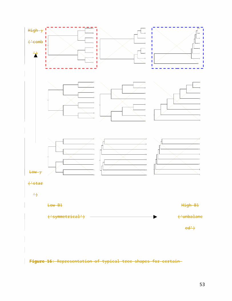
Figure 16: Representation of typical tree shapes for certain combinations of and B1. The NT
statistic exhibited weak power in symmetrical, comb-like trees (red dashed box). The MC
statistic exhibited weak power in unbalanced, comb-like trees (blue dashed box).
37
1

The statistics’ sensitivity to tree shape was also investigated; the MC and NT statistics both
appear to suffer from reduced power under certain conditions, illustrated in Figure 5.16. The MC
statistic was weak when trees were comb-like (internal nodes distributed toward the tips of the
tree) in balanced trees (such as in the top-right hand corner (blue box) of Figure 5.16). The NT
statistic was weak in unbalanced comb-like trees (such as in the top-left corner (red box) of
Figure 5.16). What both cases have in common is that in very comb-like trees, internodal
distances among the immediate ancestors are often minimal, reflecting low sequence
divergence. As a result, reconstructing phylogenetic relationships in these cases may be
problematic: single ML trees often represent these relationships as soft polytomies. In a
posterior set of trees this will manifest itself as a wider variation in tree branching orders.
However, both the MC and NT statistics are most sensitive to changes in branching order near
the tips of a phylogeny: the MC statistic because the largest clade monophyletic for a given trait
value in a phylogeny rarely extends deeply to the root, as can be verified by comparing the
observed MC size with number of tips in total; the NT statistic by implication since it calculates
the nearest taxon of the same trait value over all taxa – which will frequently traverse the tree no
deeper than the first or second ancestor node.
Where large variance exists this may result in lower observed mean MC clade sizes than in less
comb-like trees. Furthermore the observed MC clade sizes may be further lowered since in
unbalanced phylogenies monophyletic clades arise under a narrower range of possible trait
associations than in balanced phylogenies. To illustrate this point, consider two trees where
one, C (which might be similar to the tree in the top-left corner of Figure 5.116), is completely
symmetrical, and the other, U, is unbalanced (similar to the tree in the top-right corner of Figure
5.16). Now suppose we begin with no character traits assigned to any of the tips, and assign a
hypothetical ‘white’ trait to four of the tips in such a way as to maximise phylogeny-trait
association. However, the first ‘white’ trait must be assigned at random.
38
1
2
3
4
5
6
7
8
9
10
11
12
13
14
15
16
17
18
19
20
21
22
23
24
25
26

It can be seen that the position of the first trait value on C is irrelevant; a monophyletic clade of
‘white’ traits can still be created. However, any monophyletic clade in U must include the two
uppermost taxa. In other words, for any tree of more than three taxa, more phylogeny trait
associations leading to monophyletic clades of size two or larger are possible in balanced trees
than in unbalanced trees. The MC statistic therefore suffers from reduced power in unbalanced
comb-like trees because observed mean MC clade sizes tend to be smaller, increasing the
potential overlap between observed and null distributions.
The NT statistic is expected to correlate with strength of trait-phylogeny association because
phylogenetically related taxa should be separated by minimal evolutionary distance. This can
usefully be considered here as the sum of the two external branch lengths in question (which
will not depend on their phylogenetic proximity) and the internal branch distance separating
them, which will depend on their evolutionary relationship. In comb-like trees, the nearest-
neighbour distance between two taxa of the same trait value (as calculated in the observed NT
size) will be largely determined by their external branch lengths, since, as in the MC statistic,
they will rarely be separated by more than a few internal nodes. However, the expected NT
distances will vary, depending on the degree of tree imbalance. In symmetrical comb-like trees,
the nearest-neighbour distances of any randomly-chosen pair of taxa will vary little; in other
words, observed and expected NT values will be similar, since the distribution of possible NT
distances is relatively smooth. I therefore suggest that the power of the NT statistic could be
improved by considering only internal branch lengths. These results underscore the importance
of exploring the effect of likely parameter values on statistical power.
Furthermore, on reflection the distance-based statistics (UF, NT, NR and PD) may generally
suffer from another drawback. The null distribution for all these statistics is calculated by
39
1
2
3
4
5
6
7
8
9
10
11
12
13
14
15
16
17
18
19
20
21
22
23
24
25
26
random allocation of trait values on the tips of the phylogeny (see Chapter Two, specifically
Section 2.3.1Parker et al., 2008 - Methods). Effectively, this method only randomizes the
association of trait values with branching order, not branch length. The null hypothesis is that
there is no evolutionary association between taxa with identical trait values; that two taxa are as
likely to have the same trait value if they are selected at random or if they share phylogenetic
ancestry.
Where shared phylogenetic ancestry is represented by common topology (as in the AI, PS and
MC statistics introduced previouslyin Chapter Two) it is necessary and sufficient to generate the
null distribution through randomizing branch orders since power to reject the null hypothesis
arises from lower-than-expected numbers of internal nodes separating associated traits.
However, in the case of statistics that incorporate branch length information (as in the UF, PD,
NT & NR statistics introduced in this chapter) it may not be sufficient to simply randomize
branching order as in Chapter TwoParker et al. (2008) to calculate a null distribution. A more
appropriate null distribution would randomize both branch order and branch lengths in the tree –
Freckleton & Pybus (2006) followed a similar approach to test trait association. Alternatively, a
new phylogeny could be generated de novo. Pybus and Harvey (2000) used birth-death models
to usefully simulate phylogenetic trees; alternatively the coalescent (Kingman 1982a, b) might
provide a suitable null model. Clearly further work is needed to establish how the null
distribution for distance-based phylogeny-trait association statistics may be most efficiently
calculated.
WeI have developed this technique in order to take advantage of Bayesian MCMC processes
that more adequately estimate the true topology of a phylogeny, as they incorporate
phylogenetic error in the estimation process through the posterior set of trees. In Chapter
TwoParker et al. (2008) it was not important to accurately estimate the substitution model and
40
1
2
3
4
5
6
7
8
9
10
11
12
13
14
15
16
17
18
19
20
21
22
23
24
25
26

molecular clock model, since the measures of phylogeny-trait association (AI, PS, MC) were
purely topological.
However with respect to phylogeny-trait association statistics incorporating branch length
information (PD, NT & NR, UF) branch lengths must be more accurately estimated. This
presents a challenge since model selection procedures in Bayesian MCMC methods are
laborious and in the process of development. That is, although Bayesian MCMC methods
explore the parameter space of a given substitution model well, the actual choice of model used
may be subject to misspecification (Suchard et al., 2001). Since these measures depend on
accurate branch length estimation, misspecification of the substitution model may lead to
serious consequences for the accuracy of these statistics.
Accordingly, weI suggest that the best available model selection procedures should be followed
when these statistics are used to quantify phylogeny-trait association. Furthermore, work needs
to be done to quantify the sensitivity of these statistics to substitution model misspecification.
More generally, this conclusion (and the result seen in Chapter Three, where a large number
of substitution models tested disagreed in predicted substitution rates ) strongly suggests
that substantial further work is needed to put model selection in Bayesian MCMC phylogenetic
analyses on a more rigourously-tested footing, with commonly-accepted standards of model
selection.
In conclusion, this study suggests that a combination of PD, UF AI and PS statistics should be
used in studies of phylogeny-trait association. These combine correct Type I error rates,
reasonable power that is evenly spread across the range of tree shapes tested, and utilize both
branching order (topology) and length (in the case of UF and PD) information.
ACKNOWLEDGEMENTS
41
1
2
3
4
5
6
7
8
9
10
11
12
13
14
15
16
17
18
19
20
21
22
23
24
25
26
JDP was funded by the UK Natural Environment Research Council (xxx). OGP was
funded by XXXX (xxx)
42
1
2

ReferencesREFERENCES
Bhattacharya T, Daniels M, Heckerman D, Foley B, Frahm N, Kadie C, Carlson J, Yusim K, McMahon B, Gaschen B, Mallal S, Mullins JI, Nickle DC, Herbeck J, Rousseau C, Learn GH, Miura T, Brander C, Walker B, Korber B. (2007) Founder effects in the assessment of HIV polymorphisms and HLA allele associations. Science 315:1583-6.
Carrington, C.V.F., Foster, J.E., Pybus, O.G., Bennett, S.N. & Holmes, E.C. (2005). Invasion and maintenance of Dengue Virus Type 2 and Type 4 in the Americas. J. Virol. 79(23): 14680-14687.
Colless, D.H. (1982) Phylogenetics: the theory and practice of phylogenetic systematics. Part II, pp. 100–104.
Drake, J. W., Charlesworth. B., Charlesworth, D. & Crow, J. F. (1998) Rates of spontaneous mutation. Genetics 148:1667-1686.
Drummond, A. J. & Rambaut, A. (2007) BEAST: Bayesian evolutionary analysis by sampling trees. BMC Evol. Biol. 7:214-226.
Faith, D.P. (1992) Conservation evaluation and phylogenetic diversity. Biol. Cons. 61:1-10.
Fitch, W.M. (1971b). Toward defining the course of evolution: Minimal change for a specific tree topology. Syst. Zool. 20: 406-416.
Freckleton, R. P. & Harvey, P. H. (2006) Detecting non-brownian trait evolution in adaptive rasiations. PLoS Biol. 4(11):3373.
Fu, Y. X. & Li, W. H. (1993) Statistical tests of neutrality of mutations. Genetics 48:91-103.
Fulcher, J.A., Hwangbo, Y., Zioni, R., Nickle, D., Lin, X., Heath, L., Mullins, J.I., Corey, L. & Zhu, T. (2004). Compartmentalization of Human Immunodeficiency Virus Type 1 between blood monocytes and CD4(+) T cells during infection. Journal of Virology, 78(15):7883-7893.
Grenfell, B. T., Pybus, O. G., Gog, J. R., Wood, J. L. N., Daly, J. M., Mumford, J. A. & Holmes, E. C. (2004) Uniting the epidemiological and evolutionar dynamics of pathogens. Science 303:327-332.
Holmes, E.C. (2004). The phylogeography of human viruses. Molecular Ecology 13:745-756.
Jenkins, G.M., Rambaut, A., Pybus, O.G. & Holmes, E.C. (2002) Rates of molecular evolution in RNA viruses: A quantitative phylogenetic analysis. J. Mol. Evol. 54:156-165.
Kingman, J. F. C. (1982a) The coalescent. Stoch. Proc. App. 13:235-248.
Kingman, J. F. C. (1982b) On the genealogy of large populations. J. Appl. Probab. 19A:27-43.
Kirkpatrick and Slatkin (1993). M. Kirkpatrick and M. Slatkin, Searching for evolutionary patterns in the shape of a phylogenetic tree. Evolution 47 :1171–1181.
Komatsu H, Lauer G, Pybus OG, Ouchi K, Wong D, Ward S, Walker B & Klenerman P. (2006).
43
1
23456789
1011121314151617181920212223242526272829303132333435363738394041424344454647484950

Do antiviral CD8+ T cells select hepatitis C virus escape mutants? Analysis in diverse epitopes targeted by human intrahepatic CD8+ T lymphocytes. Journal of Viral Hepatitis 13:121-30.
Leigh Brown, A.J., Lobidel, D., Wade, C.M., Rebus, S., Philips, A.N., Brettle, R.P., France, A.J., Leen, C.S., McMenamin, J., McMillan, A., Maw, R.D., Mulcahy, F., Robertson, J.R., Sankar, K.N., Scott, G., Wyld, R. & Peutherer, J.F. (1997). The molecular epidemiology of human immunodeficiency virus Type 1 in six cities in Britain and Ireland. Virology 235:166-177.
Lilliefors, H. W. (1969) On the Kolmogorov-Smirnov test for Normality with mean and variance unknown. J. Am. Stat. Ass. 62(318):399-402.
Lozupone, C. & Knight, R. (2005) UniFrac: A new method for comparing microbial communities. App. & Environ. Microbiol. 71(12):8228-8235.
Massey, F. J. (1951) The Kolmogorov-Smirnov test for goodness of fit. J. Am. Stat. Ass. 46(253):68-78.
McKenzie, A., & Steel, M (2000) Distributions of cherries for two models of trees. Math. Biosci. 164: 81–92.
Nakano, T., Lu, L., Liu, P. & Pybus, O.G. (2004). Viral gene sequences reveal the variable history of hepatitis C virus infection among countries. Journal of Infectious Disease 190:1098-1108.
Parker, J. D., Rambaut, A., Pybus, O.G. (2008). Correlating viral phenotypes with phylogeny: accounting for phylogenetic uncertainty. Infect. Genet. Evol. 8(3):239-246.
Pillai, S.K., Kosakovsky Pond, S.L., Lui, Y., Good, B.M., Strain , M.C., Ellis, R.J., Letendre, S., Smith, D., Gunthard, H.F., Grant, I., Marcotte, T.D., McCutchan, J.A., Richmann, D. & Wong, K. (2006). Genetic attributes of cerebrospinal fluid-derived HIV-1 env. Brain 129: 1872-1883.
Potter, S. J. , Lemey, P., Achaz, G., Chew, C. B., Vandamme, A.-M., Dwyer, D. E. & Saksena, N. K. (2004) HIV-1 compartmentalization in diverse leukocyte populations during antiretroviral therapy. J. Leukocyte. Biol. 76:562-570.
Pybus OG & Harvey PH (2000) Testing macro-evolutionary models using incomplete molecular phylogenies. Proc Roy Soc B 267:2267-2272.
Rambaut, A. & Grassly, N.C. (1997). Seq-Gen: an application for the Monte Carlo simulation of DNA sequence evolution along phylogenetic trees. Bioinformatics 13(3):235-238.
Rambaut, A. (2001). Phyl-O-Gen. Available at http://evolve.zoo.ox.ac.uk
Salemi, M., Lamers, S.L., Yu, S., de Oliveira, T., Fitch, W.M. & McGrath, M.S. (2005). Phylodynamic analysis of Human Immunodeficiency Virus Type 1 in distinct brain compartments provides a model for the neuropathogenesis of AIDS. J. Virol 79(17): 11343-11352.
Sheridan I, Pybus OG, Holmes EC, Klenerman P. (2004). High resolution phylogenetic analysis of hepatitis C virus adaptation and its relationship to disease progression. Journal of Virology 78:3447-54.
44
123456789
101112131415161718192021222324252627282930313233343536373839404142434445464748495051

Slatkin, M., & Maddison, W.P. (1989). A cladistic measure of gene flow measured from the phylogenies of alleles. Genetics 123(3):603-613.
Sobesky, R., Feray, C., Rimlinger, F., Derian, N., Dos Santos, A., Roque-Alonso, A.-M., Samuel, D., Bréchot, C. & Thiers, V. (2007) Distinct hepatitis C virus core and F protein quasispecies in tumoral and nontumoral hepatocytes isolated via microdissection. Hepatology 46:1704-1712.
Starkman, S.E., MacDonald, D.M., Lewis, J.C.M., Holmes, E.C. & Simmonds, P. (2003). Geographic and species association of hepatitis B virus genotypes in non-human primates. Virology 314:381-393.
45
123456789
10111213
Sullivan, S.T., Mandava, U., Evans-Strickfaden, T. et al. (2005). Diversity, divergence, and evolution of cell-free Human Immunodeficiency Virus Type 1 in vaginal secretions and blood of chronically infected women: associations with immune status. Journal of Virology, 79 (15): 9799-9809.
Suchard, M.A., Weiss, R.E. & Sinsheimer, J.S. (2001) Bayesian selection of continuous-time Markov chain evolutionary models. Mol. Biol. Evol. 18:1001:1013.
Wang, T.H., Donaldson, Y.K., Brettle, R.P., Bell, J.E. & Simmonds, P. (2001). Identification of shared populations of Human immunodeficiency Virus Type 1 infecting microglia and tissue macrophages outside the central nervous system. J. Virol. 75 (23): 11686-11699.
Webb, C.O. (2000) Exploring the phylogenetic structure of ecological communities: an example for rain forest trees. Am. Nat. 156(2):145-155
Webb, C.O., Ackerly, D.D, McPeek, M.A. & Donoghue, M.J. (2002) Phylogenies and community ecology. Annu. Rev. Ecol. Syst. 33:475-505
46
123456789
101112131415161718
19
20
21

TABLES
Statistic Type I rate
AI 0.051
PS 0.046
UF 0.028
PD 0.041
NR 0.062
NT 0.041
MC 0.029
Table 1: Type I error rate of statistics implemented in the Befi-BaTS package. Error rate given is
the proportion of significant results (p 0.05) observed in a data set of 897 randomly assigned
tip trait values (binary character, 10,000 shuffles).
47
1
2
3
4
5
6
7
Patient 1
= -2.34, B1 = 35.5
Patient 7
= 3.20, B1 = 35.4
Statistic1
Mean
posterior
estimate
95 % HPD2
(lower,
upper) P3
Mean
posterio
r
estimate
95 % HPD2
(lower,
upper) P3
AI 2.83 2.07, 3.58 0.000 0.03 0.00, 0.09 <0.005
PS 29.72 25, 34 0.000 6.03 4, 8 <0.005
UniFrac 0.45 0.38, 0.52 0.010 0.85 0.77, 0.92 0.010
NT 442
373.16,
516.11 0.000 60.18
45.29,
76.86 <0.005
NR 17330
14185,
20894 0.090 2324 1758, 2984 <0.005
PD 1400 1193, 1631 0.000 290
226.12,
361.47 <0.005
MCN1 1.57 1, 2 0.080 9.96 10, 10 0.010
MCN2 2.09 2, 3 0.190 5.93 6, 6 0.010
MCserum 4.36 3, 6 0.270 31.33 31, 33 0.010
MCtumour 4.09 2, 7 0.010 10.85 6, 15 0.010
48
1

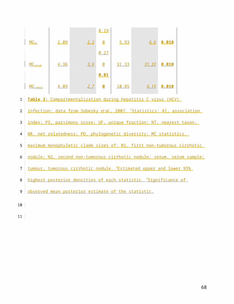
Table 3: Compartmentalization during hepatitis C virus (HCV) infection; data from Sobesky et
al., 2007. 1 Statistics: AI, association index; PS, parsimony score; UF, unique fraction; NT,
nearest taxon; NR, net relatedness; PD, phylogenetic diversity; MC statistics, maximum
monophyletic clade sizes of: N1, first non-tumorous cirrhotic nodule; N2, second non-tumorous
cirrhotic nodule; serum, serum sample; tumour, tumorous cirrhotic nodule. 2 Estimated upper and
lower 95% highest posterior densities of each statistic. 3 Significance of observed mean posterior
estimate of the statistic.
49
1
2
3
4
5
6
7
8
9

FIGURES
Figure 1: Trees a) and b) have identical topologies. The association between the ‘red’ and
‘black’ traits and phylogeny, as measured by the AI statistic, is necessarily the same for both.
50
1
2
3
4
5

Figure 2: The trees presented in Figure 2; this time phylogeny-trait association is measured by
four statistics (UniFrac, Nearest Taxon (‘NT’), Net Relatedness (‘NR’) & Phylogenetic Diversity
(‘PD’)). The value of the statistic is proportional to the strength of association; higher values are
more strongly associated. Tree b) has stronger phylogeny-trait association than tree a).
51
1
2
3
4
5
6

High
(‘comb’)
Low
(‘star’)
Low B1
(‘symmetrical’)
High B1
(‘unbalanced’)
Figure 3: Diagram of the spread of tree shapes represented by the nine master topologies used
in simulation, ordered by their node spread ( statistic, vertical axis) and tree imbalance, (B1,
horizonal axis).
52
1
2
3
4
53
1
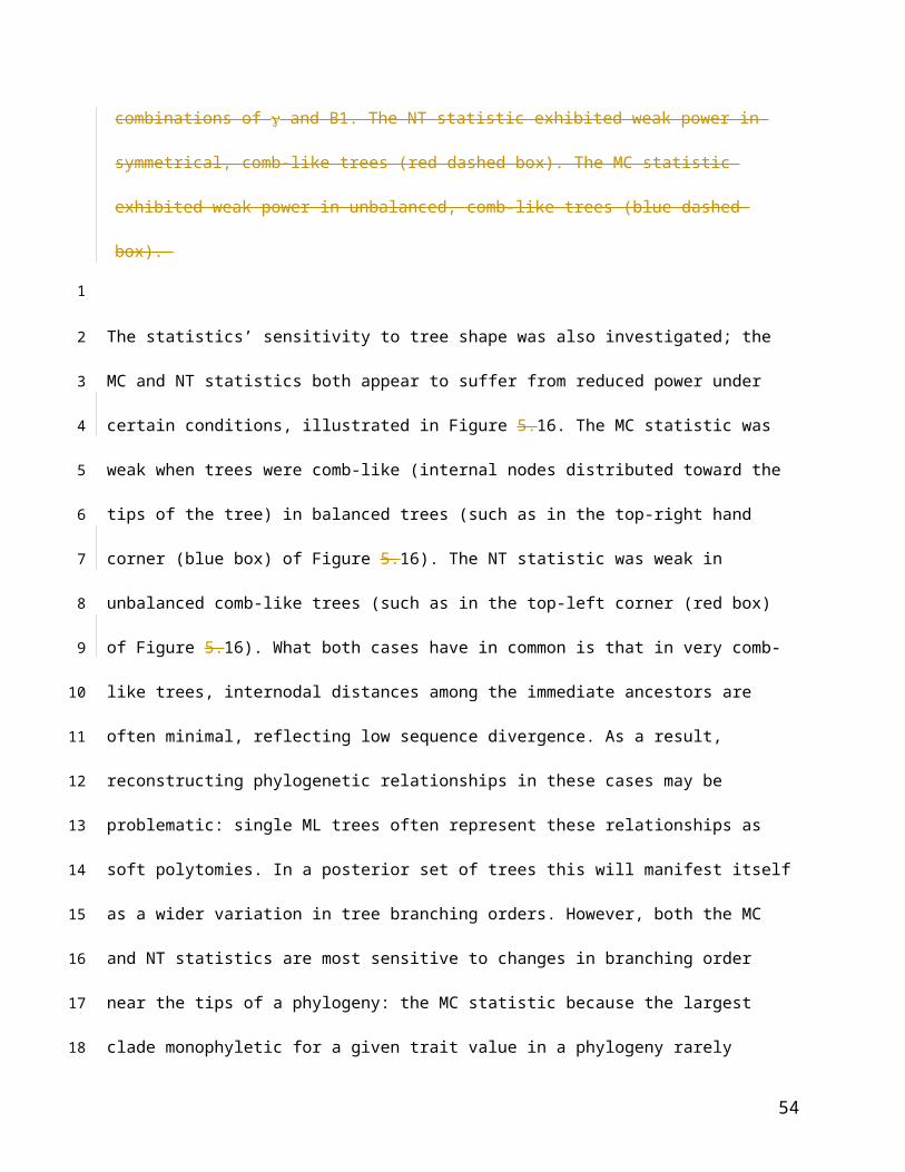
Figure 4: CDFs and performance of AI statistic on simulated data. Top panel: CDFs of each
simulation, from no shuffles, or completely associated (red) to 10,000 shuffles (violet). The unity
(unit uniform distribution) is shown in grey. Centre panel: proportion of simulations rejecting H0
(out of 897 possible) with increasing trait re-arrangements (log10). Lower panel: mean
significance of observed AI statistic.
54
1
2
3
4
5
6

Figure 5: CDFs and performance of parsimony statistic (PS) on simulated data. Top panel:
CDFs of each simulation, from no shuffles, or completely associated (red) to 10,000 shuffles
(violet). The unity (unit uniform distribution) is shown in grey. Centre panel: proportion of
simulations rejecting H0 (out of 897 possible) with increasing trait re-arrangements (log10). Lower
panel: mean significance of observed parsimony statistic.
55
1
2
3
4
5
6

Figure 6: CDFs and performance of unique fraction (UniFrac) statistic on simulated data. Top
panel: CDFs of each simulation, from no shuffles, or completely associated (red) to 10,000
shuffles (violet). The unity (unit uniform distribution) is shown in grey. Centre panel: proportion
of simulations rejecting H0 (out of 897 possible) with increasing trait re-arrangements (log10).
Lower panel: mean significance of observed UniFrac statistic..
56
1
2
3
4
5
6

Figure 7: CDFs and performance of phylogenetic diversity (PD) statistic on simulated data. Top
panel: CDFs of each simulation, from no shuffles, or completely associated (red) to 10,000
shuffles (violet). The unity (unit uniform distribution) is shown in grey. Centre panel: proportion
of simulations rejecting H0 (out of 897 possible) with increasing trait re-arrangements (log10).
Lower panel: mean significance of observed PD statistic.
57
1
2
3
4
5
6

Figure 8: CDFs and performance of nearest taxon (NT) statistic on simulated data. Top panel:
CDFs of each simulation, from no shuffles, or completely associated (red) to 10,000 shuffles
(violet). The unity (unit uniform distribution) is shown in grey. Centre panel: proportion of
simulations rejecting H0 (out of 897 possible) with increasing trait re-arrangements (log10). Lower
panel: mean significance of observed NT statistic.
58
1
2
3
4
5
6
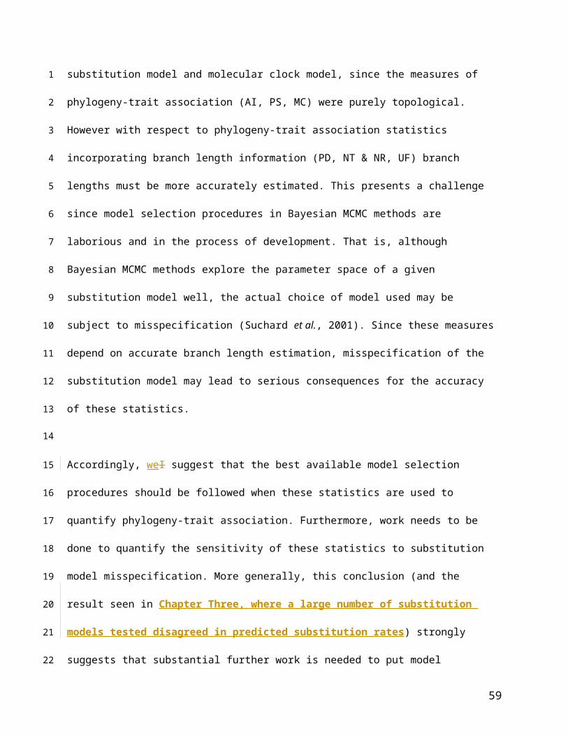
Figure 9: CDFs and performance of net relatedness (NR) statistic on simulated data. Top
panel: CDFs of each simulation, from no shuffles, or completely associated (red) to 10,000
shuffles (violet). The unity (unit uniform distribution) is shown in grey. Centre panel: proportion
of simulations rejecting H0 (out of 897 possible) with increasing trait re-arrangements (log10).
Lower panel: mean significance of observed NR statistic.
59
1
2
3
4
5
6

Figure 10: CDFs and performance of MC statistic on simulated data. Top panel: CDFs of each
simulation, from no shuffles, or completely associated (red) to 10,000 shuffles (violet). The unity
(unit uniform distribution) is shown in grey. Centre panel: proportion of simulations rejecting H0
(out of 897 possible) with increasing trait re-arrangements (log10). Lower panel: mean
significance of observed MC statistic.
60
1
2
3
4
5

61
1

Figure 11: The CDF for each statistic was compared to a unit uniform distribution under
increasing numbers of taxon rearrangements using a Kolmogorov-Smirnoff test. Shown are the
value of the difference statistic (lower plot) and p-value (upper plot) in each separate simulation
replicate (log10(taxon rearrangements)).
62
1
2
3
4
5

Figure 12: Proportion of rejections of H0 (p 0.05) with increasing numbers of random taxon
trait-value rearrangements (log scale) in different statistics. The dashed red line is at 0.05 (5%),
the proportion of trials expected to reject H0 under the null hypothesis at = 0.05 if the Type I
error rate is correct.
63
1
2
3
4

Figure 13: Mean significance of observed trait-association values by different statistics with increasing numbers of random taxon trait-value rearrangements (log scale).
64
1
23

Figure 14: Distribution of tree shape statistics of 897 simulated data sets used in this study.
Each alignment was simulated from one of nine master topologies picked to give a range of tree
topologies typical of human immunodeficiency virus (HIV) evolution. Simulated alignments were
analysed in BEAST version 1.4.6 (see Methods for details). Mean tree shape statistics given
were calculated from the posterior set of trees (PST) in each analysis using code from the
FigTree version 1.1 package (retrieved from http://beast-mcmc.googlecode.com; my
implementation is available on request).
65
1
2
3
4
5
6
7
8
910
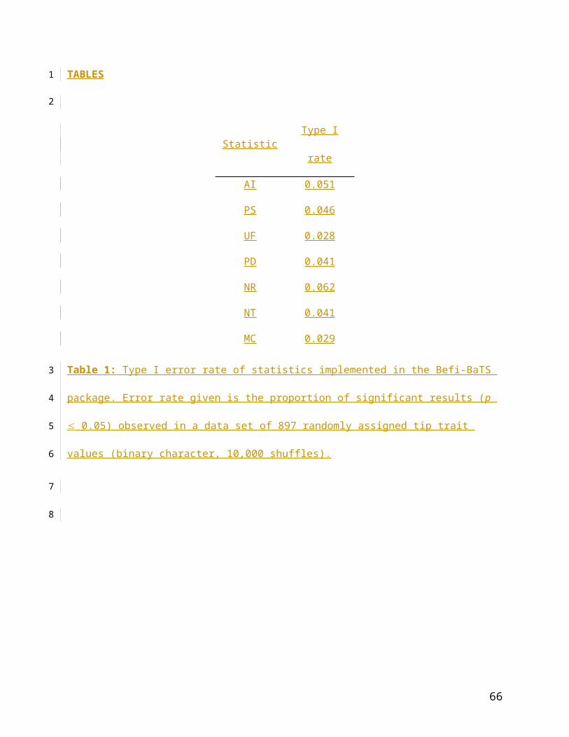
Figure 15a: Variation of statistical power with tree shape for various phylogeny-trait association
statistics. Higher (Pybus & Harvey, 2000) values indicate trees where the distribution of
nodes is skewed towards the tips of the phylogeny; Higher B1 values (Kirkpatrick & Slatkin,
1992) indicate greater node imbalance. ‘P’, the significance of each data set in the totally
associated model.
66
1
2
3
4
5
6
7
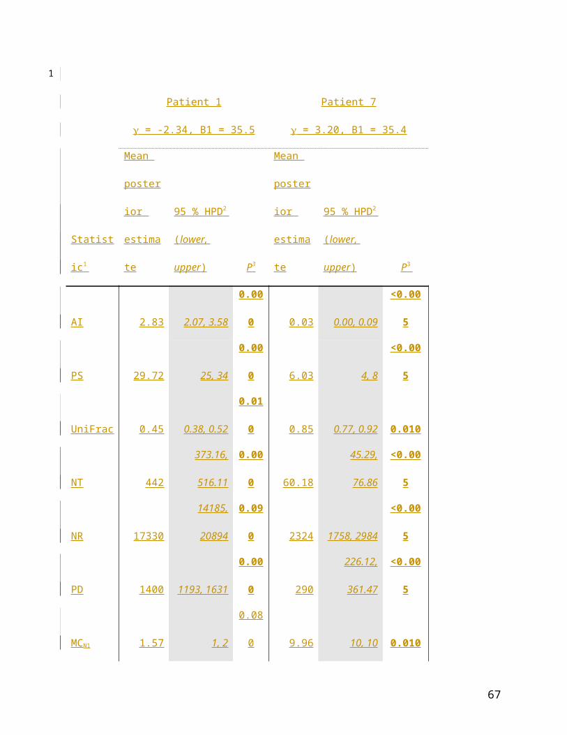
Figure 15b: A more detailed look at dependence of power on tree shape in MC and NT
statistics. The MC statistic, left, shows weaker power in trees with strong node imbalance (high
B1 statistic) and a distribution of nodes that is skewed towards the tips of the tree (high ). The
NT statistic, right, is also weaker in topologies with high , but in trees with evenly-balanced
nodes.
67
1
2
3
4
5
6
7
High
(‘comb’)
Low
(‘star’)
Low B1
(‘symmetrical’)
High B1
(‘unbalanced’)
Figure 16: Representation of typical tree shapes for certain combinations of and B1. The NT
statistic exhibited weak power in symmetrical, comb-like trees (red dashed box). The MC
statistic exhibited weak power in unbalanced, comb-like trees (blue dashed box).
68
1
2