error analysis for the in-situ fabrication of mechanisms

tur-e thatr of

mainnce ofde in

n. Inanced sto-d isherare

Sanjay Rajagopalane-mail: [email protected]

Mark Cutkoskye-mail: [email protected]

Center for Design Research,Stanford University,

Palo Alto, CA 94305-2232

Error Analysis for the In-SituFabrication of MechanismsFabrication techniques like Solid Freeform Fabrication (SFF), or Layered Manufacing, enable the manufacture of completely pre-assembled mechanisms (i.e. thosrequire no explicit component assembly after fabrication). We refer to this mannebuilding assemblies as in-situ fabrication. An interesting issue that arises in this dois the estimation of errors in the performance of such mechanisms as a consequemanufacturing variability. Assumptions of parametric independence and stack-up maconventional error analysis for mechanisms do not hold for this method of fabricatiothis paper we formulate a general technique for investigating the kinematic performof mechanisms fabricated in-situ. The technique presented admits deterministic anchastic error estimation of planar and spatial linkages with ideal joints. The methoillustrated with a planar example. Errors due to joint clearances, form errors, or oteffects like link flexibility and driver-error, are not considered in the analysis—butpart of ongoing research.@DOI: 10.1115/1.1631577#

r

iy,n

e

o

h

e

q

n

e

m

-ex-rees.

bri--atedh-atha-een

ue,

rc-ay

ng aiefit asain

d

1 IntroductionThe last decade of the millennium has seen the widesp

adoption of new ‘‘freeform’’ fabrication techniques. Called bvarious names~Rapid Prototyping, Layered Manufacturing, SolFreeform Fabrication etc.!, this technology builds a part directlfrom its digital ~CAD! representation by ‘‘slicing’’ the part modeland building it incrementally by selectively adding and removimaterial@1# @2# @3#.

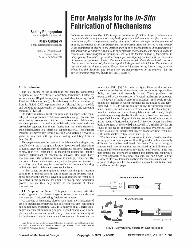
Of particular interest for the purposes of this paper is the cability of these processes to fabricate assemblies~e.g., mechanismswith mating components! in-situ. In conventional fabrication,each component of a device is individually fabricated and thassembled together. Forin-situ fabrication, the entire device isbuilt encapsulated in a sacrificial support material. This suppmaterial is removed~by etching, melting, or dissolving it away! toyield the final part with operational mating and fitting featur~see Fig. 1!.

This paper examines the manner in which manufacturing errspecifically errors in the spatial location~position and orientation!of joints, affect the performance of mechanical devices fabricain-situ. It is well established in theoretical kinematics that tprimary determinant of mechanism behavior~for rigid bodymechanisms! is the spatial location of its joints@4#. Consequently,the focus of mechanism error analysis techniques on paramvariability ~e.g. link length! is an artifact of the manufacturingtechniques used to fabricate these mechanisms.

In this paper, an assumption is made that the joint locatvariability is process-specific, and is taken as the primary exenous factor to the analysis. Given this assumption, the technipresented in this paper are not unique to any specific fabricaprocess, nor are they only limited to the analysis of plamechanisms.

1.1 Scope of the Paper. This paper is concerned with thstudy of general~i.e. planar or spatial, open-chain or multi-loop!mechanisms, fabricated using freeform techniques.

As students in kinematics classes soon learn, the fabricatioprecise mechanism prototypes can be a complex, time-consuand sometimes, frustrating task. It is believed that Charles Bbage’s mechanical computing engine, a good example of a cplex spatial mechanism, failed mainly because of the inabilityits fabricators to avoid accumulated component dimensional

Contributed by the Mechanisms and Robotics Committee for publication inJOURNAL OF MECHANICAL DESIGN. Manuscript received March 2002; reviseApril 2003. Associate Editor: J. S. Rastegar.

Copyright © 2Journal of Mechanical Design

eadyd

g

pa-

en

ort

s

rs,

tede

tric

ionog-ues

tionar

n ofing

ab-om-ofer-

rors in the 1800s@5#. The problems typically occur due to inaccuracies in mechanism dimensions, poor joints, out-of-plane flibility in links and assembly issues. These problems aexacerbated in the construction of spatial mechanism prototyp

The advent of Solid Freeform Fabrication~SFF! could revolu-tionize the manner in which mechanisms are designed and facated@6# @7# @8#. In-situ technology allows for precision components, sensors, actuators and electronics to be directly integrinto the mechanism frame during fabrication. Alternately, higprecision joints may also be directly built by freeform processesa specified location. Figure 2 shows examples of some mecnisms recently fabricated at Stanford University. Others have bbuilt at Rutgers University@9# and Laval@10#. Similar devices arefound in the realm of microelectromechanical systems~MEMS!which also use an incremental layered manufacturing techniqwith much smaller feature sizes~see Fig. 3!.

Whether at microscopic or macroscopic scales,in-situ manufac-turing practices have a process flow~Fig. 4! that is fundamentallydifferent from either traditional ‘‘craftsman’’ manufacturing oconventional mass production. As described in the following setions, the difference in process flow leads to differences in the wthat dimensional errors are generated and accumulate, requiridifferent approach to tolerance analysis. We begin with a brreview of classical tolerance analysis for mechanisms and usea point of departure for the modified approach that is the mcontribution of this paper.

the

Fig. 1 Conventional versus in -situ fabrication

003 by ASME DECEMBER 2003, Vol. 125 Õ 809

e

-

orns.

ren-a-

tber

mp-

ofons,inkit-r-

ly ifath-

iven

are

re-

heest.

ap-as-lf,.ble

nEq.f a

1.2 Introducing Mechanism Error Analysis. The modernscientific treatment of mechanism error estimation dates toearly 1960’s@11# @12#. In the several decades since, many altnative approaches to error analysis for mechanisms have bproposed—each with various simplifying assumptions and diffent levels of complexity@13# @14# @15# @16# @17#. All approaches,however, attempt to solve the same basic problem—to predict thenature and amount of performance deterioration in mechanisas a result of non-ideal synthesis, fabrication, materialscomponentry.

In this paper the focus is on kinematic performance. In othwords, we assume that we are always able to describe the detask in terms of an output equation of the form:

y5 f ~F,Q! (1)

Fig. 2 In -situ mechanism prototypes fabricated via ShapeDeposition Manufacturing †3‡: „a… a polymer insect-leg proto-type with embedded pneumatic actuator, pressure sensor andleaf-spring joint „b… a hexapedal robot with integrated sensors,actuators and electronics „c… an ‘‘inchworm’’ mechanism, withintegrated clutch components, „d… a slider-crank mechanismmade from stainless steel. Images courtesy the Stanford Cen-ter for Design Research and Rapid Prototyping Laboratories.

Fig. 3 Micromechanisms and devices built using in -situ fab-rication techniques. Images courtesy Sandia National Labora-tories, SUMMiT „tm … Technologies, www.mems.sandia.gov.Used with permission.

810 Õ Vol. 125, DECEMBER 2003

ther-een

er-

msor

ersired

wherey denotes the (m31) vector of output end-effector locations, coupler-point positions or output link angles,Q is a (k31) vector of known driving inputs, andF is a (n31) vector ofindependent mechanism variables—including deterministicrandomly distributed geometric parameters and/or dimensioThe functionf (•) is called thekinematic functionof the mecha-nism and is, in general, assumed to be a continuous and diffetiable ~i.e. smooth! non-linear mapping from the mechanism prameter space to an output space~e.g. a Cartesian workspace!. Inthe absence of higher-pairs~i.e. joints that have line and poincontact, as opposed to surface contact, between their memlinks! and multiple-contact kinematics, the smoothness assution generally holds true.

1.3 Conventional Mechanism Error Analysis. Conven-tional error analysis deals with degradation in the performancea mechanism as a result of parametric or dimensional variatiand play in joints. The parameters typically considered are llengths for planar linkages, or some form of the DenavHartenberg@18# parameters for spatial linkages. Error in the peformance of known mechanisms can be estimated analyticalcertain assumptions are made, rendering the underlying mematical treatment more tractable. For example:

• Mechanism dimensions and parameters have a known, gvariability characteristic—either deterministic, or stochastic.

• Dimensional/parametric variations and clearance valuessignificantly smaller than their nominal values.

• Individual component variations are independent, uncorlated and identically distributed.

• The output is, at most, a weak non-linear function of tmechanism parameters at the operating configuration of inter

As a result of these assumptions, it becomes possible toproximate the actual error by lower-order estimates. Othersumptions~e.g. negligible variability of the clearance value itseNormal or Uniform distribution of component parameters etc!,which either eliminate unnecessary model complexity or enaanalytical tractability, are also commonly made.

1.3.1 Sensitivity Analysis.Sensitivity analysis is based othe Taylor-series expansion of the output function. As stated in~1!, the end-effector position, coupler path or output angle omechanism can be expressed as:

y5 f ~F,Q! (2)

Fig. 4 Comparing conventional and in -situ manufacturingmethods—process flow chart. Actions that impart accuracy tothe mechanism are specifically identified.

Transactions of the ASME

y

n

t

a

.cr

n

.c

io

O

ilitynotier tod

in-ouslso

eth-w-

be

heceptb-tive

ni-iquebi-

aa-inhas

talhilebe

-uc-

tos-

on

trib-de-

ech-ade

is

ntas

whereQ[@u1 ,u2 , ¯ ,uk#T are thek known driving inputs, and

F[@f1 ,f2 , ¯ ,fn#T are then mechanism parameters~or di-mensions! subject to random, or worst-case deterministic, vaability. SinceQ is assumed static for a given mechanism configration ~i.e. the driving inputs are held perfectly to their nominvalues!, it is dropped from the equation for notational simplicitThe previous equation is re-written as:

y5 f ~F! (3)

Expanding this function in Taylor-series around the nomivalues of the mechanism parameters (Fnom

[@f1nom,f2

nom, ¯ ,fnnom#T), we get:

y5 f ~Fnom!1(i 51

n] f

]f iG

nom

~f i2f inom!1

1

2! (i 51

n]2f

]f i2G

nom

~f i

2f inom!21(

i . j

]2f

]f i]f jG

nom

~f i2f inom!~f j2f j

nom!1¯

(4)

or, using a more concise notation:

y5 f ~Fnom!1] f

]FGnom

~F2Fnom!11

2!

]2f

]F2Gnom

~F2Fnom!21¯

(5)

For small, independent variations about the nominal configution, a linear approximation can be made—thereby rewritingabove equation as:

y' f ~Fnom!1] f

]FGnom

~F2Fnom! (6)

or

Dy'] f

]FGnom

DF (7)

The quantity] f /]F] nom is known as thesensitivity Jacobianofthe mechanism, evaluated at the nominal configuration. This Jbian relates the component variability (DF) in the mechanismparameter space to the output variation (Dy) in Cartesian spaceThis is classical sensitivity analysis, where all variational effeare bundled into a simple parametric space, and all higher oeffects are neglected.

Equation~7! is used as the basis for error analysis and toleraallocation. For error analysis, the component variability (DF) andsensitivity Jacobian (] f /]F) are known for a given mechanismconfiguration. The output error (Dy) is then a simple calculationThe component variability can either be expressed as worst-values, or as stochastic variations in link parameters. Eachthese approaches is discussed in the next sections.

For tolerance allocation problems, the maximum permissoutput error (Dy

max) and sensitivity Jacobian are known. Equati~7! forms the basis for the constraint equations, and the objecis to maximize the overall variability~i.e. DF), given the con-straints. Greater allowable variability typically means lowmanufacturing and inspection costs, and thus, is preferred.simple formalization of the tolerance allocation problem isfollows:

minimize Z5(i 51

n1

DF(8)

subject to:

g~F![Dymax2

] f

]FGnom

DF<0 and

gi~F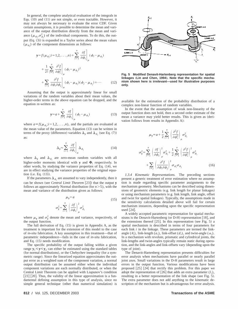![f i>0; i 51,2, . . . ,n. (9)

Journal of Mechanical Design

ri-u-al.

al

ra-he

co-

tsder

ce

aseof

blentive

erne

as

Here, an assumption is made that each component variabparameter is weighted equally in the cost function, which mayalways be true. Some manufacturing parameters may be eascontrol accurately than others~e.g. hole size can typically be helto tighter tolerances than center-distance between holes!. Addi-tionally, zero tolerance~or close-to-zero tolerance! for some pa-rameters, which is permissible for the above formalization, isfeasible for real manufacturing processes. Non-homogenemanufacturing capability within the mechanism workspace is anot considered in this system.

The optimization problem can be solved using standard mods of parametric programming—Lagrange multipliers, or Poell’s conjugate direction method~i.e. unconstrained optimizationof a penalty function! @19#. An example of these optimizationtechniques applied to mechanism tolerance allocation canfound in @20#.

1.3.2 Deterministic, Worst-Case Error Estimation.In worst-case error estimation, each parameterf i is assumed to take~ex-clusively! one of two deterministic valuesf i

min andf imax. Further-

more, it is assumed thatf imin<fi

nom<f imax;i51,2, . . . ,n, where

f inom is the nominal value of thei th parameter.The objective of this kind of error estimation is to determine t

worst case envelope of the mechanism performance error. Exfor applications where performance within specified limits is asolutely critical, the worst-case analysis results in conservaestimates of error~and thereby, over-design of components!. Sincethe worst performance can occur for any combination of mimum and maximum component parameter values, the technproceeds by exhaustive calculation of total error for each comnation of individual error values. Forn parameters, this leads tosearch space of 2n combinations for each mechanism configurtion. If the objective is to find the worst-case performance withthe entire workspace of the mechanism, then this calculationto be repeated at each incremental driver position.

An alternative approach is to use dynamic programming@21#@22# to estimate the maximum error without computing the toerror for every possible combination. The assumption made wusing this technique is that the global optimization problem canre-stated as a multi-stage optimization problem, with thenth stagesolution related to the (n21)th stage solution through a functional equation. While this technique results in significant redtion of the computational burden involved, it is not guaranteedfind the global optimum when the underlying monotonicity asumptions do not hold.

1.3.3 Stochastic Error Estimation.Statistical error estima-tion proceeds by assigning a probability distribution functi~PDF! to each variable parameterf i . The component dimensionunder consideration is assumed to be a random variable, disuted according to the characteristics of its underlying PDF,noted aspFi

(f i). The cumulative distribution function~CDF! ofthe output functions can then be estimated using standard tniques for stochastic analysis. If certain assumptions can be m~e.g. linearity, independence, identical distribution etc.!, the esti-mation of the distribution and moments of the output functionhighly simplified.

The error equation~Eq. ~7!! can be replaced by an equivaleequation for the stochastic estimation of each output CDF,follows:

PYj~yj !5E

2`

f1

. . . E2`

fn

yj .pF1 . . . Fn~f1 , . . . ,fn!df1 . . . dfn

where j 51,2, . . . ,m (10)

and for independent and uncorrelatedf i

pF1 . . . Fn~f1 , . . . ,fn!5)

i 51

n

pFi~f i ! (11)

DECEMBER 2003, Vol. 125 Õ 811

s

iv

u

a

d

a

a

n

on

e

p-en-

ion

-

r-

-

rel

e-s.

In general, the complete analytical evaluation of the integralEqs. ~10! and ~11! are not simple, or even tractable. However,may not always be necessary to evaluate the error CDF. Gcertain assumptions, it is possible to determine the mean andance of the output distribution directly from the mean and vaance (mf i

,sf i

2 ) of the individual components. To do this, the ouput ~Eq. ~3!! is expanded in a Taylor series about the mean val(mf i

) of the component dimensions as follows:

y5 f ~mf i; i 51,2, . . . ,n!1(

i 51

n] f

]f iG

m

~f i2mf i!

11

2! (i 51

n]2f

]f i2G

m

~f i2mf i!2

1(i . j

]2f

]f i]f jG

m

~f i2mf i!~f j2mf j

!1¯ (12)

Assuming that the output is approximately linear for smvariations of the random variables about their mean values,higher-order terms in the above equation can be dropped, anequation re-written as:

y'a1(i 51

n] f

]f iG

m

~f i2mf i! (13)

wherea[ f (mf i; i 51,2, . . . ,n), and the partials are evaluated

the mean value of the parameters. Equation~13! can be written interms of the proxy~difference! variablesDy andDf i

~see Eq.~7!!

as:

Dy'(i 51

n] f

]f iG

m

Df i(14)

where Dy and Df iare zero-mean random variables with a

higher-order moments identical withy and Fi respectively. Inother words, by studying the variance properties of Eq.~14!, weare in effect studying the variance properties of the original eqtion ~i.e. Eq.~13!!.

If the parametersDf iare assumed to vary independently, then

can be shown~seeCentral Limit Theorem@23#! that the outputyfollows an approximately Normal distribution~for n.5), with themean and variance of the distribution given as follows:

my5a(15)

sy25(

i 51

n S ] f

]f iD

m

2

sf i

2

wheremy andsy2 denote the mean and variance, respectively,

the output function.The full derivation of Eq.~15! is given in Appendix A, as the

treatment is important for the extension of this model to the cof in-situ fabrication. A key assumption in this treatment—thatparametric independence—fails in the case ofin-situ fabrication,and Eq.~15! needs modification.

The specific probability of the output falling within a giverangey1<y<y2 can either be estimated using the standard tab~for normal distributions!, or the Chebychev inequality~for a sym-metric range!. Since the linearized equation approximates the oput error as a weighted sum of the component variation, a noroutput distribution can be assumed either when the individcomponent variations are each normally distributed, or whenCentral Limit Theorem can be applied with Liapunov’s conditi@23# @20#. Thus, the validity of the linear approximation is a fudamental defining assumption in this type of analysis, sincesimple general technique~other than numerical simulation! is


initvenari-ri-t-es

llthethe

t

ll

ua-

it

of

seof

les

ut-malualthen-no

available for the estimation of the probability distribution of acomplex non-linear function of random variables.

In the event that the assumption of weak non-linearity of theoutput function does not hold, then a second order estimate of thmean a variance may yield better results. This is given as~deri-vation follows from results in Appendix A!:

my5a11

2 (i 51

n S ]2f

]f i2D

m

sf i

2

sy25(

i 51

n S ] f

]f iD

m

2

sf i

2 11

2 (i 51

n S ]2f

]f i2D

m

2

sf i

2

1(iÞ j

S ]2f

]f i]f jD

m

2

sf isf j

(16)

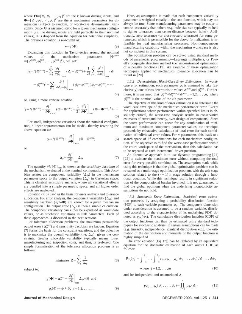
1.3.4 Kinematic Representations.The preceding sectionspresent a generic treatment of error estimation where no assumtion is made regarding specific parameter assignments to thmechanism geometry. Mechanisms can be described using dimesions of geometric elements~e.g. link length for planar linkages!or using mechanism parameters~e.g. link length, link angle, offsetand twist for spatial linkages!. Typically, the assumptions made inthe sensitivity calculations detailed above will fail for certainmechanism instances, depending upon the specific representatused@24#.

A widely accepted parametric representation for spatial mechanisms is the Denavit-Hartenberg~or D-H! representation@18#, andthe extensions thereof@25#. In this representation~see Fig. 5! aspatial mechanism is described in terms of four parameters foeach link i in the linkage. These parameters are termed the linkangle (u i), link-length (ai), link-offset (di), and twist-angle (a i).In a mechanism with revolute, prismatic and cylindrical joints, thelink-lengths and twist-angles typically remain static during operation, and the link-angles and link-offsets vary~depending upon thetype of joint!.

The Denavit-Hartenberg representation presents difficulties foerror analysis when mechanisms have parallel or nearly paralljoint axes. Small variations in the D-H parameters result in largeerrors in the output function. Various modifications have beenproposed@25# @24# that rectify this problem. For this paper weadopt the representation of@26# that adds an extra parameter (l i),resulting in a better representation of the link shape~see Fig. 5!.The extra parameter does not add anything to the kinematic dscription of the mechanism but is advantageous for error analysi

Fig. 5 Modified Denavit-Hartenberg representation for spatiallinkages „Lin and Chen, 1994 …. Note that the specific mecha-nism shown here is irrelevant—used for illustrative purposesonly.


Journal of Mechanic

Fig. 6 The effects of link length variation in an assembled 4-bar mechanism

oen

s,,

n

hi

ts

l

i

,

monisde-

bri-

ha-nd 7rios,

e

e is

the

-

n

isified

tes

e

r-

2 Worst-Case Error Analysis for In-Situ FabricationThe conventional error models presented in Sec. 1.3 canno

directly applied toin-situ fabrication since this fabrication technique differs from conventional sequential shape-and-assemfabrication techniques in some fundamental ways. Primarily,differences are:

• In-situ fabrication is blind to conventional component bounaries. Consequently, the input to the analysis is not the dimsional variability in links, but the absolute position and orientativariability in joints. As the assembly is built, joints are creatdirectly or embedded within a surrounding matrix of part asupport material. Links are formed around the joints. Paramevariability is therefore a function of joint placement accuracy.

• Tolerance stack-up due to dimensional/parametric errorcomponents is not an issue forin-situ fabrication. Instead, jointsand other features such as coupler points or end-effectorsplaced in the workspace with a known absolute accuracy.

• Gaps and clearances in joints are manifest directly ingeometry of the support structure. In conventional fabrication,gap geometry is a consequence of the interaction amocomplementary mating/fitting feature geometries.

• Conventional error analysis does not explicitly allow for tconsideration of variable accuracy within the manufacturworkspace. But when entire mechanisms are fabricatedIn-situ, thebuild configuration~or pose! can be chosen to make best usethe manufacturing error characteristics.

These differences are accounted for in the general absmodel for in-situ fabrication and the associated error analytechniques presented below.

2.1 An Abstract Model for In-Situ Fabrication. The maindifference between conventional error analysis, and error anafor in-situ fabrication lies in the form of the inputs into the modeConventional error analysis treats parametric variability~i.e. vari-ability in link-lengths etc.! as a given constant input.In-situ erroranalysis estimates parametric variability for each build configution from the location variability of the joints that make up thlinkage. The parametric variability is determined by the sensitivof each parameter to the joint positions and orientations at a gbuild pose. An important observation is that the mechanismrameters that result from such fabrication are not independent

al Design

t be-ble

the

d-en-ndd

tric

in

are

thethegst

eng

of

ractis

ysisl.

ra-eityvenpa-but

pair-wise correlated. This is because multiple~adjacent! param-eters depend upon the same independent inputs~i.e., the positionsand orientations of their shared joints!. Although several param-eters can all be adjacent to each other if they share a comjoint, their correlation is still taken pair-wise since covariancedefined on random variable pairs. The degree of correlationpends upon the configuration in which the mechanism is facated~also called thebuild pose!. The output variability, in turn, isdetermined by the sensitivity of the output function to the mecnism parameters at each operating configuration. Figures 6 aillustrate the fundamental differences between the two scenafor the simple case of a four-bar mechanism.

2.2 Frames and Notation. We assign a global workspacdatum frame (OXYZ) and local datum frames (oixiyizi) associ-ated with each feature of interest,~see Fig. 8!. Without loss ofgenerality, it can be assumed that the z-axis of the global framaligned with the process growth direction~e.g. vertical, or spindle-axis!. If the feature of interest is a joint, then it is assumed thatlocal joint z-axis (zi for the i th joint! is aligned with the joint-freedom axis~i.e. nominal pin/shaft axis for revolute joints, direction of translational motion for prismatic joints etc.!. The directionof the x-axis of thei th frame (xi) is taken as that of the commonormal between thei th and~adjacent! i 21th nominal joint axes.

Typically, the position and orientation of each feature framespecified in the global frame, and the feature geometry is specin the local frame. The nominal location of the origin in thei thlocal frame is represented as the position vectorpi in the globalframe ~or alternately, as the homogeneous coordina@xi ,yi ,zi ,1#), and the nominal orientation of thei th frame is rep-resented by the direction vectorzi ~with direction numbers@ l i ,mi ,ni #). Alternately, the z-axis of the joint frame can buniquely represented in a global frame in terms of its Plu¨cker @27#coordinates (Qi ,Q8 i), where:

Qi[@q1i ,q2i ,q3i # (17)

are the direction numbers, and:

Q8 i[pi3Qi[@q1i8 ,q2i8 ,q3i8 # (18)

is the moment vector of the line. Furthermore, we can letq1i2

1q2i2 1q3i

2 51 without any loss of generality, making these coodinates the same as thedirection cosinesof the line.

Fig. 7 The effects of joint location variation for an in -situ fabricated 4-barmechanism


a

b

ameers tople

ofed

ex-as

lityom

-

,

ethe

ion

ksi-

put

Thus, using this representation, the nominal configurat(Cnom) of a mechanism can be represented in terms of the loframe positions and orientations as:

Cnom[$~pinom,zi

nom!%; i 51,2, . . .n (19)

or alternately, in terms of the joint-axis Plu¨cker coordinates as:

Cnom[$~Qi ,Q8 i !%; i 51,2, . . .n (20)

Fabrication proceeds by constructing or embedding non-idjoints at the given nominal locations. By quantifying the extentthese errors, it is possible to predict overall performance errormechanisms fabricatedin-situ. The complete procedure is described in later sections~Secs. 2.4 and 3!.

2.3 Heterogeneous Workspace Modeling. For modelingvariable fabrication accuracy within the process workspace,assume that we have aprecision function~t! that returns the vari-ability region R of a joint in the build space, given the nominposition and orientation, and other process parameters~p!. Notethat the precision functiont is process-specific and needs toempirically determined for each process, such as SDM, FD

Fig. 8 Frames and notation for the abstract model of in -situfabrication


ioncal

ealofs in-

we

l

eM,

SLS, Stereolithography etc. The variability region is simplyworst-case or stochastic characterization of the variation in fraposition and orientation, given its nominal location and othprocess-specific parameters. While this methodology extendthe general spatial scenario, it is illustrated here with a simplanar example.

2.3.1 Planar Example. In the planar case, the orientationsthe joint axes~i.e. zi) are discarded, as all joint axes are assumparallel. Given a nominal joint locationpnom[(xnom,ynom), theprecision function returns a regionR as follows:

R5t~xnom,ynom,p! (21)

In deterministic worst-case analysis, this function returns thetremal positions of the region in which the actual joint lies,follows:

R5@worst2case,xmin,xmax,ymin,ymax# (22)

Similarly, in stochastic analysis, the function returns a probabidistribution that describes the position of the point as a randvariable, as follows:

R5@normal,mx ,sx2 ,my ,sy

2# (23)

In the most general case,R is a closed region of arbitrary geometry within which the actual joint position (x,y) lies with a knownprobability distribution. By applying the precision functiont to allthe joint and coupler points (xi

nom,yinom) in a planar mechanism

we get joint variability regionsRi as:

Ri5t~xinom,yi

nom,p! (24)

In other words, the regionsRi determine the characteristics of thinterval or random values that represent the variable nature ofjoint locations. The mechanism parametersf i are functions~e.g.distance function of the formf i5$((xi2xj )

2%1/2) of the posi-tions and orientations, and the parametric variability is a functof the joint variability regions (Ri), all at the given build configu-ration (Cb):

Df i5Df i

~R1 ,R2 , . . .Rn!; i 51,2, . . .n (25)

Error analysis involves estimating the variability in the linparametersf i using the above equation, and then applying sentivity analysis techniques to determine the error in the outfunction ~at various operating configurations! for a mechanism

Fig. 9 Actual and schematic diagrams of the planar 4-bar crank-rocker mechanism used as anexample in this paper. The parameter values are: L 1Ä15 cm, L 2Ä5 cm, L 3Ä25 cm, L 4Ä20 cm, L 5Ä7.5 cm, L 6Ä20 cm „after Mallick and Dhande, 1987 …. Stochastic simulations onthe example are performed with a positional variance sx k

2 Ä0.01 cm2. Worst case simulationsare performed with a positional variability of 0.3 cm, equivalent to the 3 s stochastic error.


Journal of Mechanical D

Fig. 10 Multiple positions of the example 4-bar mechanism, correspondingto 30 deg increments of the input angle, u

ic

e

luo

a

uild

rst-

sild2

-d a

the, fore-

ionnal

ut

ma-ild

s ine-ureonig.ld

ler

bothap-rior

that is fabricatedin-situ. In the following sections, this processdescribed, and illustrated using the specific planar 4-bar menism shown in Fig. 9. The mechanism parameter values wchosen to allow checking of results with earlier published wo@28#. However, in that case, the authors consider a clearanceof 0.05 cm in the joints, along with a 0.5 percent error in linlength. Since neither link variability or clearance are variabin our analysis, the comparison is qualitative. To aid with discsion of the results, the mechanism is also shown in variconfigurations~i.e. specific values of the driving angleu! in Fig.10. In Sec. 4, the analysis is extended to cover general spmechanisms.

Fig. 11 An example build configuration and worst-case varia-tions in joint and coupler point locations

esign

sha-ererkrrorkess-us

tial

2.4 Error Estimation. Worst case error estimation forin-situ fabrication proceeds in two stages. First, at a candidate bposeCb , all the worst case parameter values (f i

WC) are evaluatedby choosing, in sequence, all possible combinations of the wocase fabrication input values$(pi

WC ,ziWC)%.

The precision function~Eq. ~24!! returns these extremal valueof the position of each joint, given the mechanism nominal bupose. Fork fabrication input variables, this process generatesk

candidate mechanisms at each poseCb . Figure 11 shows the example of a mechanism with 3 mm square precision regions ancandidate build configuration.

In the second stage, the error in the output function~y! is evalu-ated for each one of the candidate mechanisms produced infirst stage. This calculation is repeated for all operating anglesevery build pose. Overall, ifc operating and build positions arconsidered for a mechanism withm independent degrees of freedom, andk independent fabrication variables, the determinatof worst-case error boundaries for the output has computatiocomplexity O(2kmc2). Dynamic programming approaches@22#can significantly improve upon the computational complexity, bneed to be re-stated appropriately for each specific problem.

Figure 12 illustrates the results of the worst-case error estition for the example 4-bar mechanism for a few candidate buposes. The coupler-point location is shown as a cloud of pointthe vicinity of the nominal coupler-point, with each point corrsponding to one combination of worst-case joint locations. Fig13 plots the worst-case variability of the coupler-point locati~i.e. half the perimeter of the bounding box for each cloud in F12! as a function of the build configuration. Of the four buiconfigurations evaluated, the one corresponding tou5180 deg isevidently best for minimizing the worst-case errors in coupposition.

3 Stochastic Error Analysis for In-Situ FabricationThe worst-case method presented in the previous section is

overly conservative, and computationally expensive for mostplications. By contrast, a stochastic approach results in supe


816

Fig. 12 Worst case coupler-point positional error, plotted on the coupler path

r

c

l

l

t

mbleom-nand

thelus-s

int-ou-

rac-ano-ri-

error estimates in constant-time~as opposed to exponential or linear time for worst-case methods!. However, the conventional approach to stochastic error estimation needs modification in oto be applicable toin-situ fabrication.

In this analysis, we assume that the joint coordinates~positionsand orientations! are independent random variables with knowdistributions. Given the nominal location of a jointi , the precisionfunction ~Eq. ~24!! returns the appropriate distribution for its atual location. Mechanism parameters~like link-lengths, jointangles, joint offsets and skew angles! are functions of the inde-pendent, random joint coordinates. This, in turn, makes the pareters themselves random variables which are pairwise corre~being jointly dependent on the same independent variables!. Theoutput, then, is a complex function of correlated random variab

The probability distribution~i.e. PDF! of a known function ofrandom variables can, in principle, be derived exactly from

Õ Vol. 125, DECEMBER 2003

--der

n

-

am-ated

es.

he

given, analytically specified, distributions of the original randovariables. However, in practice, the exact derivation is intractain the absence of certain simplifying assumptions, due to the cplexity of the algebra involved. For a weakly non-linear functioof independent and uncorrelated random variables, the meanvariance of the function can be approximated directly frommean and variance of the underlying random variables, as iltrated in Eqs.~15! and ~16!. When the simplifying assumption~i.e. independent and uncorrelated! do not hold, the function prop-erties need to be determined analytically by integrating the joPDF~see Eq.~28!!, by modifying the approximation techniques tinclude the effects of correlation, or by using Monte Carlo simlation techniques. In general, the analytical technique is not ttable for all but the simplest of cases. In the following section,improved approximation technique for the estimation of the mments of a weakly-nonlinear function of correlated random va

Fig. 13 Total worst-case coupler-point positional errors, plotted against operating angle for fourdifferent build configurations, corresponding to different values of the input angle. The error valuescan be compared with 3 s stochastic errors „see Fig. 17 ….


Journal of

Fig. 14 First order estimates of the link-length variance compared to the results of a Monte Carlosimulation

j

n

s

e-n

w

ah

tin

ob-yle

veryon

plepicare

thef a

ionions of

ying

a-m

he

ed

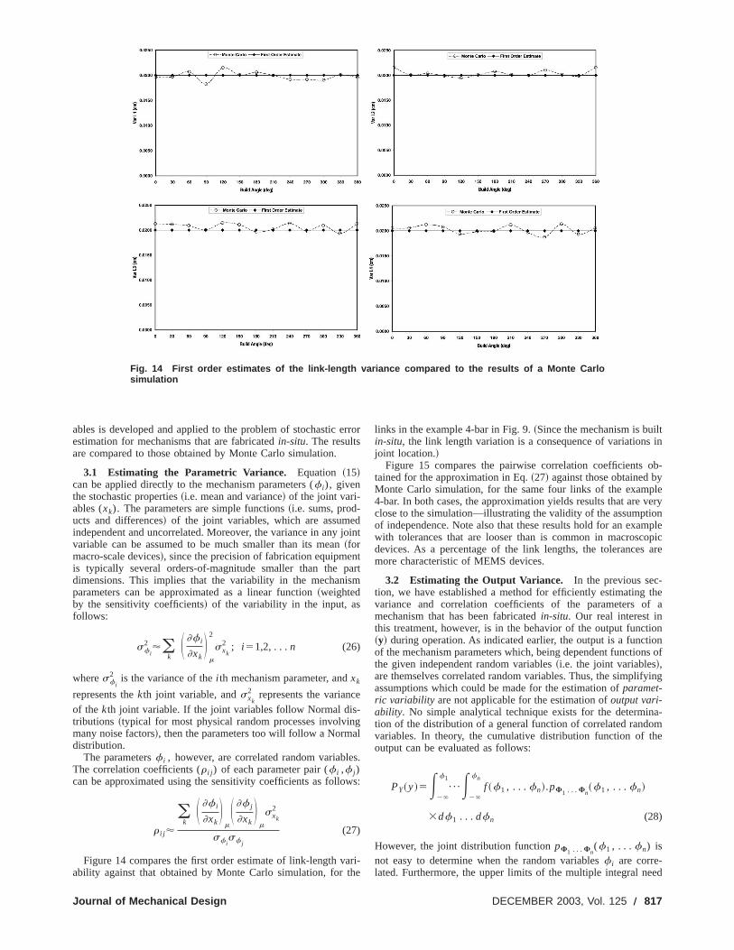
ables is developed and applied to the problem of stochastic eestimation for mechanisms that are fabricatedin-situ. The resultsare compared to those obtained by Monte Carlo simulation.

3.1 Estimating the Parametric Variance. Equation ~15!can be applied directly to the mechanism parameters (f i), giventhe stochastic properties~i.e. mean and variance! of the joint vari-ables (xk). The parameters are simple functions~i.e. sums, prod-ucts and differences! of the joint variables, which are assumeindependent and uncorrelated. Moreover, the variance in anyvariable can be assumed to be much smaller than its mean~formacro-scale devices!, since the precision of fabrication equipmeis typically several orders-of-magnitude smaller than the pdimensions. This implies that the variability in the mechaniparameters can be approximated as a linear function~weightedby the sensitivity coefficients! of the variability in the input, asfollows:

sf i

2 '(k

S ]f i

]xkD

m

2

sxk

2 ; i 51,2, . . .n (26)

wheresf i

2 is the variance of thei th mechanism parameter, andxk

represents thekth joint variable, andsxk

2 represents the variancof the kth joint variable. If the joint variables follow Normal distributions ~typical for most physical random processes involvimany noise factors!, then the parameters too will follow a Normadistribution.

The parametersf i , however, are correlated random variableThe correlation coefficients (r i j ) of each parameter pair (f i ,f j )can be approximated using the sensitivity coefficients as follo

r i j '

(k

S ]f i

]xkD

mS ]f j

]xkD

m

sxk

2

sf isf j

(27)

Figure 14 compares the first order estimate of link-length vability against that obtained by Monte Carlo simulation, for t

Mechanical Design

rror

doint

tartm

gl

s.

s:

ri-e

links in the example 4-bar in Fig. 9.~Since the mechanism is builin-situ, the link length variation is a consequence of variationsjoint location.!

Figure 15 compares the pairwise correlation coefficientstained for the approximation in Eq.~27! against those obtained bMonte Carlo simulation, for the same four links of the examp4-bar. In both cases, the approximation yields results that areclose to the simulation—illustrating the validity of the assumptiof independence. Note also that these results hold for an examwith tolerances that are looser than is common in macroscodevices. As a percentage of the link lengths, the tolerancesmore characteristic of MEMS devices.

3.2 Estimating the Output Variance. In the previous sec-tion, we have established a method for efficiently estimatingvariance and correlation coefficients of the parameters omechanism that has been fabricatedin-situ. Our real interest inthis treatment, however, is in the behavior of the output funct~y! during operation. As indicated earlier, the output is a functof the mechanism parameters which, being dependent functionthe given independent random variables~i.e. the joint variables!,are themselves correlated random variables. Thus, the simplifassumptions which could be made for the estimation ofparamet-ric variability are not applicable for the estimation ofoutput vari-ability. No simple analytical technique exists for the determintion of the distribution of a general function of correlated randovariables. In theory, the cumulative distribution function of toutput can be evaluated as follows:

PY~y!5E2`

f1

¯E2`

fn

f ~f1 , . . .fn!.pF1 . . . Fn~f1 , . . .fn!

3df1 . . . dfn (28)

However, the joint distribution functionpF1 . . . Fn(f1 , . . .fn) is

not easy to determine when the random variablesf i are corre-lated. Furthermore, the upper limits of the multiple integral ne


818 Õ Vol.

Fig. 15 Pairwise correlation coefficients of the link lengths—first-order results compared to the MonteCarlo simulation

s

-

-

t

sc

cc

ait

the

nalthe

ion.

rror

teson-adeimates-is

nifi-

thehesti-n

up-thentedcon-y de-

hes in

il-altas-een

to be expressed in terms of the output variables, which isanalytically feasible except for the simplest of cases.

The assumption that makes this problem tractable, once agis that of weak-nonlinearity in the output function. In other wordif we can assume that the second and higher-order terms inTaylor Series expansion of the output function can be discardthen it is possible to derive an expression that directly produceapproximate estimate for the output variance, given the varia(sf i

2 ) and correlation coefficients (r i j ) of the mechanism parameters. Furthermore, if the total number of parameters is large~i.e.n.5), then, according to the Central Limit Theorem, the outpfunction will follow an approximately Normal distribution, regardless of the individual parameter distributions@23#. Thus, bymaking the linear approximation, we completely side-stepevaluation of the extremely problematic multiple integral in E~28!. The derivation of the approximation equation is givenAppendix A, and the final result is summarized below:

sy2'(

i 51

n S ] f

]f iD

m

2

sf i

2 12(i

(j

] f

]f iG

m

] f

]f jG

m

r i j sf isf j

(29)

where i 51,2, . . .n and j Þ i . In the special case where onlyad-jacent parameters share a joint variable,r i j 50 for non-adjacentparameters, and the above equation needs to be evaluated onthe cases wherej 5 i 21. Note that all the sensitivity coefficientin the above equation are evaluated at the nominal operatingfiguration~m! of the mechanism. Comparison of Eq.~29! and Eq.~15! reveals that they differ only in the second term on the RHThis term, then, is the adjustment term that accounts for therelation effect that results from the co-dependence of the menism parameters on the same joint coordinates.

Summarizing, the first order approximations are the only trtable, general purpose estimates of the output function variabEquation ~29! indicates that the output error depends uponoutput function sensitivity coefficients~evaluated at the nominaoperating configuration!, the parametric variances, and the pawise correlation coefficients of the parameters. The parame

125, DECEMBER 2003

not

ain,s,theed,an

nce

ut

heq.in

ly for

on-

S.or-ha-

c-lity.helir-tric

variances and the correlation coefficients are functions ofmechanism build pose, duringin-situ fabrication. Equation~29!succinctly relates the fabrication workspace to the operatioworkspace, thereby presenting us with a method for evaluatingoptimal build pose, given an operational tolerance specificatThis issue is explored in more detail in@29#.

Figure 16 compares the first order estimated coupler-point efor the example 4-bar fabricatedin-situ against the Monte Carlosimulations of the same quantity. Also included are the estimausing the conventional approach, which does not include the csideration of correlation effects. Comparisons can also be mbetween these results, and those of the worst case error estpresented earlier~see Fig. 13!. The worst-case and stochastic etimates for a specific build angle are compared in Fig. 17. Itclear from the comparison that the worst-case method is sigcantly more conservative in its estimation of output error.

Figure 18 plots the simulated coupler-point variance againstnumber of random trials. This helps with the estimation of tminimum number of trials needed in order for the random emates to converge to a steady value~between 4000 and 10,000 ithis case!.

4 Extension to Spatial ParametersWhile the detailed treatment of spatial error analysis, with s

porting numerical results, is beyond the scope of this paper,theoretical extension of the error analysis techniques preseabove to spatial systems is straightforward once the essentialcepts have been established. Spatial systems are traditionallscribed in terms of the Denavit-Hartenberg parameters~see Sec-tion 1.3.4!, or modifications thereof. Spatial error analysis is tprocess of relating variability in the spatial parameters to errorthe output function.

For in-situ fabrication, parametric variability is not directlyavailable, but is a function of the position and orientation variabity in joint placement. Earlier sections in this paper have dewith the issue of estimating the output variance, given the stochtic characteristics of the joint variables. The approach has b


Journal of Mechan

Fig. 16 First order estimates of coupler-point variance for the an in -situ fabricatedcrank-rocker mechanism „Fig. 9 … using conventional stochastic analysis, analysismodified to for in -situ fabrication, and direct Monte Carlo simulation

csl

illustrated using a planar example, and the technique is extenhere to cover general spatial mechanisms. The basic issueremains to be addressed for the spatial case is that of expliexpressing the spatial parameters illustrated in Fig. 5 in termthe joint-frame positions illustrated in 8. This is a fairly simpproblem in the analytical geometry of three dimensions@30#.

Given the origin coordinates (pi ,pj ,pk) and the direction num-bers (zi ,zj ,zk) of the axes of threeadjacent spatially locatedjoints, the modified Denavit-Hartenberg parameters of thej thjoint can be expressed in terms of the joint Plu¨cker coordinates~see Section 2.1! of the three joint axes (Qi ,Q8 i), (Qj ,Q8 j ) and(Qk ,Q8k), and those of the two common normals (Qi j ,Q8 i j ) and(Qjk ,Q8 jk). This notation is illustrated in Fig. 19. The directiocoordinates of the common normal are given as:

Qi j [@q1i j ,q2i j ,q3i j # where

q1i j 5q2iq3 j2q3iq2 j

q2i j 5q3iq1 j2q1iq3 j

q3i j 5q2iq3 j2q3iq2 j (30)

ical Design

dedthatitlyof

e

n

and the moments of the common normal between axesi and j aregiven as follows~this can be extended toj andk by symmetry!:

Q8 i j [@q1i j8 ,q2i j8 ,q3i j8 # where

q1i j8 5Qi j •@~q2i j q3 j2q3i j q2 j !Q8 i2~q2i j q3i2q3i j q2i !Q8 j #

iQi j i2


iQi j i2


iQi j i2

(31)

The modified Denavit-Hartenberg parameters for linkj cannow be written as:


820 Õ Vol. 125, D

Fig. 17 Comparison of 3 s stochastic and worst-case „deterministic … error estimatesfor crank-rocker mechanism

frg

s

or-

a j5arcsin~ iQjki !

aj5Qj•Q8k1Qk•Q8 j

sin~a i !

dj5~pk2pj !•~Qjk3Qj !

iQjki2

l j5~pj2pk!•~Qjk3Qj !

iQjki2

u j5arcsin~ iQjki3iQi j i ! (32)

Since the mechanism parameters are now known in terms ojoint positions and orientations, it is possible to estimate the ein output function given the variability in joint location usintechniques similar to those outlined for the planar case earlier.process proceeds by writing the product of homogeneous tran

ECEMBER 2003

theror

Thefor-

mation matrices~three translations and two rotations!, that trans-form one local coordinate frame to the adjacent frame~the j thframe to thekth frame in this case!, as follows:

Akj 5T~0,0,dj !3R~zj ,u j !3T~aj ,0,0!3R~xj ,a j !3T~0,0,l j !

(33)

Next, the first-order Taylor Series approximation of the transfmation matrix is written as follows:

DAk5

]Akj

]djDdj

1]Ak

j

]u jDu j

1]Ak

j

]ajDaj

1]Ak

j

]a jDa j

1]Ak

j

] l jD l j

(34)

The parameter variabilities~i.e. Ddj,Du j

,Daj,Da j

and D l j) are

now either interval~for worst-case analysis! or random~for sto-

Fig. 18 Convergence rates of Monte Carlo simulations for different operationalangles


illits

lledrtse-

n-caleer

meiza-

ce-is-igngo-the

for

thet

n-

in-

-e

es,

re-

ll

e or

nces

chastic analysis! parameters, the variances and correlation coecients of which can be obtained using the relationships derivedEq. ~32!.

5 Conclusions and Future WorkA framework has been presented for reasoning about error

the performance of mechanisms that are slated to be built usthe increasingly popular ‘‘freeform’’ fabrication techniques. This achieved by formulating an abstract model for thein-situ fab-rication of mechanisms, and solving the problem of analyticestimation of the variance of the kinematic function, in the preence of correlated random parameters. The fundamental assutions in this treatment of error analysis are:

• The desired performance of the mechanism is specifiedterms of a kinematic output function, which is a continuous adifferentiable mapping from a parameter space to the operatioworkspace~usually a Cartesian space!. This assumption limits theapplication of the methods presented to linkages with lower paand ‘‘well-behaved’’ higher pairs only.

• The output is a weakly non-linear function of the inputs. Thenables a first-order Taylor Series approximation of the errorthe points of interest.

• In-situ fabrication is abstracted as a process of independinsertions of joints~which could have internal clearances! into afabrication workspace, with a known accuracy. The inaccuracyspecified as worst-case limits on position and orientation~for de-terministic error analysis! or variances with known distributions~for stochastic error analysis!.

Note that no assumptions of planarity or of homogeneity in wospace characteristics are made anywhere in the methodolAnalysis of parametric errors in spatial mechanisms has also bcovered in the theoretical formulation.

This paper demonstrates that differences in the manufactuprocess flow forin-situ fabrication leads to fundamental differences in how process input variability is manifested in the kinmatic output of a mechanism.

For stochastic analysis, the essential result is that we mustcount for correlations among adjacent links. In this paper we hapresented a modified stochastic analysis that accounts for therelations and shown that it compares favorably with numeriMonte Carlo simulations.

Although the need to consider correlations in the variabilitieslink parameters somewhat complicates the analysis,in-situ fabri-cation also affords some important advantages over conventiofabrication for reducing output variability, notably:

• Tolerances do not accumulate along serial chains.

Fig. 19 Notation for the derivation of modified Denavit-Hartenberg parameters from joint Plu ¨ cker coordinates.

Journal of Mechanical Design

ffi-in

s ining

is

als-mp-

inndnal

irs

isat

ent

is

rk-ogy.een

ring-e-

ac-vecor-

cal

of

nal

• There is the freedom to choose a build configuration that wminimize the output variability when the mechanism is inoperating configuration.

• Important functional gaps and clearances can be controdirectly, by controlling the dimensions of sacrificial suppomaterial between mating parts, rather than being a conquence of the mating of independently fabricated parts.

We surmise that it will be particularly important to take advatage of these characteristics in fabricating MEMS and meso-smechanisms, for which the process variability is typically a largpercentage of the feature size than for macroscopic devices.

These topics are the subject of ongoing investigation. Soresults on the treatment of clearances and on build pose optimtion are provided in@29#.

AcknowledgmentsWe gratefully acknowledge the support of the National Scien

Foundation~MIP 9617994! and the Alliance for Innovative Manufacturing ~AIM ! at Stanford. We are also grateful for the asstance provided by members of the Stanford Center for DesResearch and Rapid Prototyping Laboratories. Sanjay Rajapalan also thanks Jisha Menon for her generous support duringformulation of this work—some of which constitutes the basishis Ph.D. thesis at Stanford University.

Appendix: Estimation of Mean and VarianceHere, we are concerned with the approximate estimation of

mean and variance of an outputy, described in terms of its outpufunction f (•) and a set of n random parametersF[@f1 ,f2 , . . . ,fn# as follows:

y5 f ~F! (35)

where f (•) is, in general, a continuous and differentiable nolinear mapping, and the parametersF are random variables withno assumptions made about their distributions, correlations ordependence. It is assumed, however, that the functionf (•) is onlyweakly non-linear~i.e. high-order terms in it’s Taylor Series expansion can be neglected! and that the mean and variance of thparametersf i are known, and denoted as (mf i

,sf i

2 ).We begin by expanding the output function in its Taylor Seri

about the mean values of the parameters, as follows:

y5 f ~mf i; i 51,2, . . . ,n!1(

i 51

n] f

]f iG

m

~f i2mf i!

11

2! (i 51

n]2f

]f i2G

m

~f i2mf i!21(

i . j

]2f

]f i]f jG

m

~f i2mf i!~f j

2mf j!1¯ (36)

With a little bit of rearrangement, the above equation can bewritten in terms of proxy variablesDf i

as:

y5 f ~m i ; i 51,2, . . . ,n!1(i 51

n] f

]f iG

m

Df i

1(i

(j

]2f

]f i]f jG

m

Df iDf j

1O3 (37)

where Df i5f i2mf i

are zero-mean random variables, with ahigher order moments identical withf i . The termO3 stands forall terms in the Taylor Series expansion that are of third degremore, and are usually negligible.

We now go about the task of estimating the mean and variaof the output~the LHS term!, using the above equation. In thi


t

-

fip

ting

ss-

pen

ot-ess-

andrs,’’

-/

ontyp-

er-

s,’’

in

ical

ofbli-

ral

r-21,

h.

alm.,

g

ed

ic

ni-ch.

the

regard, we make use of the following results, which are basedelementary applications of theorems in the area of MathemaStatistics@23#:

E$ f ~F!%5 f ~mf i!

E$Df i%50

Var$y%5E$~y2my!2%

Cov$Df i,Df j

%5E$Df iDf j

%2E$Df i%E$Df j

% (38)

whereE$•% stands for the expected value, Var$•% stands for thevariance and Cov$•% stands for the covariance. For notationsimplicity, we denote the expected value, or mean, by the symm ~with the appropriate subscript!, and the variance by the symbos2. In addition, we use the covariance coefficient (r i j ), which isdefined as follows:

r i j [Cov$Df i

,Df j%

sf isf j

(39)

Note that21<r i j <1, and thatr i j 51 wheni 5 j andr i j 50 forindependent or uncorrelatedf i and f j . From the above equations, it is also apparent that:

Cov$Df i,Df j

%5E$Df iDf j

%, and E$Df iDf j

%5r i j sf isf j

(40)

Returning to the output expansion in Eq.~37!, and using the re-sults detailed above, we are able to write the expression forexpected value of the output function as follows:

E$y%[my' f ~mf i!101(

i(

j

]2f

]f i]f jG

m

E$Df iDf j

% (41)

or, using Eq.~40!:

E$y%[my' f ~mf i!1(

i(

j

]2f

]f i]f jG

m

r i j sf isf j

(42)

Equation~42! is a general expression for the approximation of tmean of a functionf (•) of random variables, which are—ingeneral—correlated.

In a manner similar to the earlier analysis, we can use Eq.~37!to write an expression for the output variance as follows:

Var$y%[sy25E$~y2my!

2%5EH S (i 51

n] f

]f iG

m

Df i

1(i

(j

]2f

]f i]f jG

m

Df iDf j D 2J

5(i

(j

] f

]f iG

m

] f

]f jG

m

E$Df iDf j

%1O3 (43)

Combining Eq.~43! with Eq. ~40!,

sy2'(

i 51

n S ] f

]f iD

m

2

sf i

2 12(i

(j

] f

]f iG

m

] f

]f jG

m

r i j sf isf j

, iÞ j

(44)

Equation ~44! is a general expression for the approximationthe variance of a function of correlated random variables. Theterm in the RHS expression is the variance assuming indedent and uncorrelated parameters. The second term applie


onical

alboll

the

he

ofrsten-s an

adjustment to the variance estimate from the first term, accounfor any correlative effects.

References@1# Beaman, J. J., 1997,Solid Freeform Fabrication: A New Direction in

Manufacturing—With Research and Applications in Thermal Laser Proceing, Kluwer Academic Publishers, Boston.

@2# Chua, C. K., and Fai, L. K., 1997,Rapid Prototyping: Principles and Appli-cations in Manufacturing, Wiley, New York, NY.

@3# Merz, R., Prinz, F. B., Ramaswami, K., Terk, M., and Weiss, L., 1994, ‘‘ShaDeposition Manufacturing,’’Proceedings of the Solid Freeform FabricatioSymposium, pages 1–8, The University of Texas at Austin, August 8–10.

@4# Bottema, O., and Roth, B., 1979,Theoretical Kinematics, Dover Publications,New York, NY.

@5# Morrison, P., and Morrison, E., 1961,Charles Babbage and His CalculatingEngines, Dover Publications, Inc., New York, NY.

@6# Cham, J., Pruitt, B. L., Cutkosky, M. R., Binnard, M., Weiss, L., and Neplnik, G., 1999, ‘‘Layered Manufacturing of Embedded Components: ProcPlanning Considerations,’’Proceedings of the 1999 ASME DETC/DFM Conference, Las Vegas, NV, September 12–15.

@7# Weiss, L. E., Prinz, F. B., Neplotnik, G., Padmanabhan, P., Schultz, L.,Mertz, R., 1996, ‘‘Shape Deposition Manufacturing of Wearable ComputeProceedings of the Solid Freeform Fabrication Symposium, University ofTexas at Austin, August 10–12.

@8# Knappe, L. F., 2000, ‘‘Building Around Inserts: Methods for Fabricating Complex Devices in Stereolithography,’’Proceedings of the 2000 ASME DETCDFM Conference, Baltimore, MD, September 10–13.

@9# Mavroidis, C., DeLaurentis, K. J., Won, J., and Alam, M., 2001, ‘‘Fabricatiof Non-assembly Mechanisms and Robotic Systems Using Rapid Protoing,’’ ASME J. Mech. Des.,123, pp. 516–519, December.

@10# Laliberte, T., Gosselin, C., and Cote, G., 2000, ‘‘Rapid Prototyping of Lowpair, Geared-pair and Cam Mechanisms,’’Proceedings of the 2000 ASMEMechanisms and Robotics Conference, Baltimore, MD, September 10–13.

@11# Tuttle, S. B., 1960, ‘‘Error Analysis,’’ Mach. Des.,32~12!.@12# Knappe, L. F., 1963, ‘‘Technique for Analyzing Mechanism Tolerance

Mach. Des., pp. 155–157, April 25.@13# Hartenberg, R. S., and Denavit, J., 1964,Kinematic Synthesis of Linkages,

McGraw Hill, New York.@14# Garrett, R. E., and Hall, A. S., 1969, ‘‘Effects of Tolerance and Clearance

Linkage Design,’’ ASME J. Eng. Ind., Series B,91, pp. 198–202.@15# Dhande, S., and Chakraborty, J., 1973, ‘‘Analysis and Synthesis of Mechan

Error in Linkages—A Stochastic Approach,’’ ASME J. Eng. Ind., Series B,95,pp. 677–680.

@16# Lakshminarayana, K., and Ramaiyan, G., 1976, ‘‘Analysis of the EffectsErrors and Clearances in Mechanisms as a Problem in Statics,’’ ASME pucation 76-DET-67,Proceedings of the ASME DETC, Montreal, Quebec,Canada, September.

@17# Tischler, C. R., and Samuel, A. E., 1999, ‘‘Prediction of Slop in GeneSpatial Linkages,’’ Int. J. Robot. Res.,18~8!, 845–858, August.

@18# Denavit, J., and Hartenberg, R. S., 1955, ‘‘A Kinematic Notation for Lowepair Mechanisms Based on Matrices,’’ ASME J. Appl. Mech., pp. 215–2June.

@19# Fox, R. L., 1971,Optimization Methods for Engineering Design, Addison-Wesley, Mass.

@20# Chakraborty, J., 1975, ‘‘Synthesis of Mechanical Error in Linkages,’’ MecMach. Theory,10, pp. 155–165.

@21# Bellman, R., 1957,Dynamic Programming, Princeton University Press,Princeton, NJ.

@22# Fenton, R. G., Cleghorn, W. L., and Fu, J., 1989, ‘‘Allocation of DimensionTolerances for Multiple Loop Planar Mechanisms,’’ ASME J. Mech., TransAutom. Des.,111, pp. 465–470, December.

@23# Feller, W., 1957,An Introduction to Probability Theory and Its Applications,Vol. 2, Wiley & Sons, New York, NY.

@24# Hayati, S., and Mirmirani, M., 1985, ‘‘Improving the Absolute PositioninAccuracy of Robot Manipulators,’’ J. Rob. Syst.,2~4!, pp. 397–413.

@25# Suh, C. H., and Radcliffe, C. W., 1978,Kinematics and Mechanism Design,Wiley and Co., New York.

@26# Lin, P. D., and Chen, J. F., 1994, ‘‘Analysis of Errors in Precision for ClosLoop Mechanisms,’’ ASME J. Mech. Des.,116, pp. 197–203, March.

@27# Stolfi, J., 1991,Oriented Projective Geometry: A Framework for GeometrComputations, Academic Press, Boston, MA.

@28# Mallik, A. K., and Dhande, S. G., 1987, ‘‘Analysis and Synthesis of Mechacal Error in Path Generating Linkages Using a Stochastic Approach,’’ MeMach. Theory,22~2!, pp. 115–123.

@29# Rajagopalan, S., 2000, ‘‘Error Analysis and Optimal Pose Selection forIn-situ Fabrication of Mechanisms,’’ Ph.D. Thesis, Stanford University.

@30# Sommerville, D. M. Y, 1959,Analytical Geometry of Three Dimensions, Cam-bridge University Press, London.


error analysis for the in-situ fabrication of mechanisms

Documents