ERDAS Imagine

OrthoBASE

Joanne Tapping Macaulay Land Use Research Institute

Contents Subject Page No.

Introduction 2

Overview of process 3

Create a new OrthoBASE project 4

Select geometric model 5

Set reference system 5

Set reference units 7

Set frame specific information 7

Adding images to the block 9

Defining the sensor 10

Interior orientation 11

Exterior orientation 13

Ground point measurement 13

Example: GCPs from Ordnance Survey LandLine data 16

Automatic tie point measurement 17

Triangulation 18

Orthoresampling 21

Appendix I. Example frame imagery 23

Appendix II Other types of imagery 25

Appendix III. Sensor specifications 27

Appendix IV. Example triangulation report 28

1

Introduction

This is a guide to the orthorectification of aerial imagery using ERDAS Imagine OrthoBASE. OrthoBASE is PC based software. The process described is for aerial frame photography, see Appendix II for details of other types of imagery. Orthorectification is the process of removing terrain distortion from imagery. Three types of data are required for the orthorectification process:

1. Digital imagery. For example scanned aerial photography or videography, to be rectified.

2. Ground control points (GCPs). GCPs can be collected from Ordnance Survey data, ground survey or from global positioning system (GPS). GCP’s are used for the referencing of the images to a map base.

3. Digital elevation model. A model of the underlying terrain is required for the removal of terrain distortion from the aerial imagery.

Sources of help and information.

• ERDAS Field Guide. The ERDAS Field Guide gives details of the theory

aspect of photogrammetry rather than details of how to do photogrammetry. The ERDAS Field Guide is available in pdf format. \IMAGINE 8.4\help\hardcopy\FieldGuide

• OrthoBASE Tour Guide. The Tour Guide leads the user through the

process using an example set of data. It is also available in pdf format. \IMAGINE 8.4\help\hardcopy\OrthoBASE_TourGuide.

• OrthoBASE Users Guide. The OrthoBASE Users Guide is also available

in pdf format. \IMAGINE 8.4\help\hardcopy\UsingOrthoBASE.

2

Overview of Process

Capture

Interior Orientation

Exterior Orientation

Ground Point Measurement

Tie Point Measurement

Triangulation

Imagery

Orthoresampling

Scanning

Figure 1. Schematic diagram of the OrthoBASE process

3

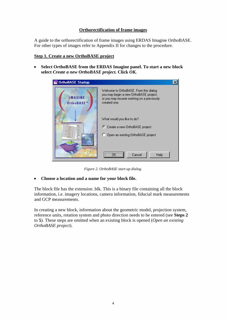
Orthorectification of frame images A guide to the orthorectification of frame images using ERDAS Imagine OrthoBASE. For other types of images refer to Appendix II for changes to the procedure. Step 1. Create a new OrthoBASE project • Select OrthoBASE from the ERDAS Imagine panel. To start a new block

select Create a new OrthoBASE project. Click OK.

Figure 2. OrthoBASE start-up dialog.

• Choose a location and a name for your block file. The block file has the extension .blk. This is a binary file containing all the block information, i.e. imagery locations, camera information, fiducial mark measurements and GCP measurements. In creating a new block, information about the geometric model, projection system, reference units, rotation system and photo direction needs to be entered (see Steps 2 to 5). These steps are omitted when an existing block is opened (Open an existing OrthoBASE project).

4

Step 2. Select Geometric Model

Figure 3. Select geometric model.

• Select Frame Camera and click OK. Step 3. Set Reference System

Figure 4. Set reference system.

• Click on the Set Projection... button.

5

Figure 5. Projection chooser. • Within the Projection Chooser dialog box select the Category required, e.g. for

the United Kingdom select United Kingdom, then for the Projection select British National Grid.

• Select the Custom tab to check or alter the details of the projection chosen.

For example, if the British National Grid projection is chosen the dialog box should be filled in as follows.

Figure 6. Defining details of the projection.

6

• Click OK to return to the Block Property Setup and then click Next to move

onto the next stage.

Figure 7. The defined reference system.

Step 4. Set Reference Units • The units for the British National Grid are meters for horizontal and vertical

units and degrees for angle units. Other projections may have different units. Check the ERDAS Field Guide for detailed descriptions of projections and units. • Click Next to move onto the next stage. Step 5. Set Frame Specific Information For most frame photography the following applies. Exception would be oblique photography, for which you would choose Y-axis for close range images.

7

Figure 8. Setting frame specific information.

• Clicking OK completes the block setup process and brings up the main

OrthoBASE dialog box. Information entered in this process can not be altered once OK has been clicked.

Add frame

Frame editor

Point measurement

Automatic tie point generation

Orthoresampling

Triangulation

Figure 9. The main OrthoBASE dialog box. Work logically through this box from left to right, i.e. Add Frame, Frame Editor, Point Measurement, Automatic Tie Point Generation, Triangulation and finally Orthoresampling.

8

Row# Left click on a row or rows within this column to select an image or

images specifically for use within OrthoBASE, e.g. computing of pyramid layers.

> Designates which image is currently active. Active X indicates which images are to be used in OrthoBASE processes such

as automatic tie point generation, triangulation and orthoresampling. Image Name Indicates the name and location of the image. Pyr. Presence (green) or absence (red) of pyramid layers. OrthoBASE

performs more efficiently if pyramid layers are present. Int. A green box indicates that the interior orientation parameters of the

images have been calculated. Ext. Green indicates that the exterior orientation parameters have been

calculated. These values are not calculated until triangulation has been run and accepted.

Online Green indicates that the images are in the correct locations. Step 6. Adding images to the block • To add images into the block select the Add images button. Select the image

required in the file list and click OK. Repeat for all images required. • To add multiple images, select the Add options tab within the file chooser.

Select the Add Selected File Plus radio button and specify a string in the Files Matching box. For example, specifying *.img adds all .img files in the folder to the block.

File types recognised include IMAGINE, TIFF, MrSID and JPEG. Refer to the Online Help documentation for a full list of supported file types.

Figure 10. Images added to the block.

In Figure 10, the images have pyramid layers associated and are in the correct location.

9

To compute pyramid layers. Select Edit and then Compute Pyramid Layers…. Choose the applicable radio button and click OK. To alter image location. Select the frame editor button. Under the Sensor tab click on Attach, reselect the location of the images and click OK. If any measurements have already been made to the images e.g. interior orientation or ground point measurement, then these will remain. Step 6. Defining the sensor. • Click on the Frame Editor button. Within the frame editor select the Sensor

tab. Information is required about the camera that obtained the images. The more information that is available the more accurate the calculations and therefore the end result will be. • Click on New… to enter the specification of the camera.

Figure 11. Specifying the sensor used to capture the imagery.

Information required: General tab Camera Name:

Description: Focal length: Principal point xo (mm): Principal point yo (mm):

Fiducials tab Required information is the number of fiducials and the

location of them on the film. Radial Lens Distortion tab Enter if information is available. For the specifications of certain cameras see Appendix III.

10

Figure 12. Entering fiducial information associated with the sensor.

• Click Save to save the camera to a .cam file that can be loaded into other

blocks. Click OK to return to the Frame Editor. Step 7. Interior Orientation This process determines the internal geometry of the camera that captured the imagery. The calculation requires principal point, focal length, fiducial marks and lens distortion.

Open viewers

Figure 13. Interior orientation.

11

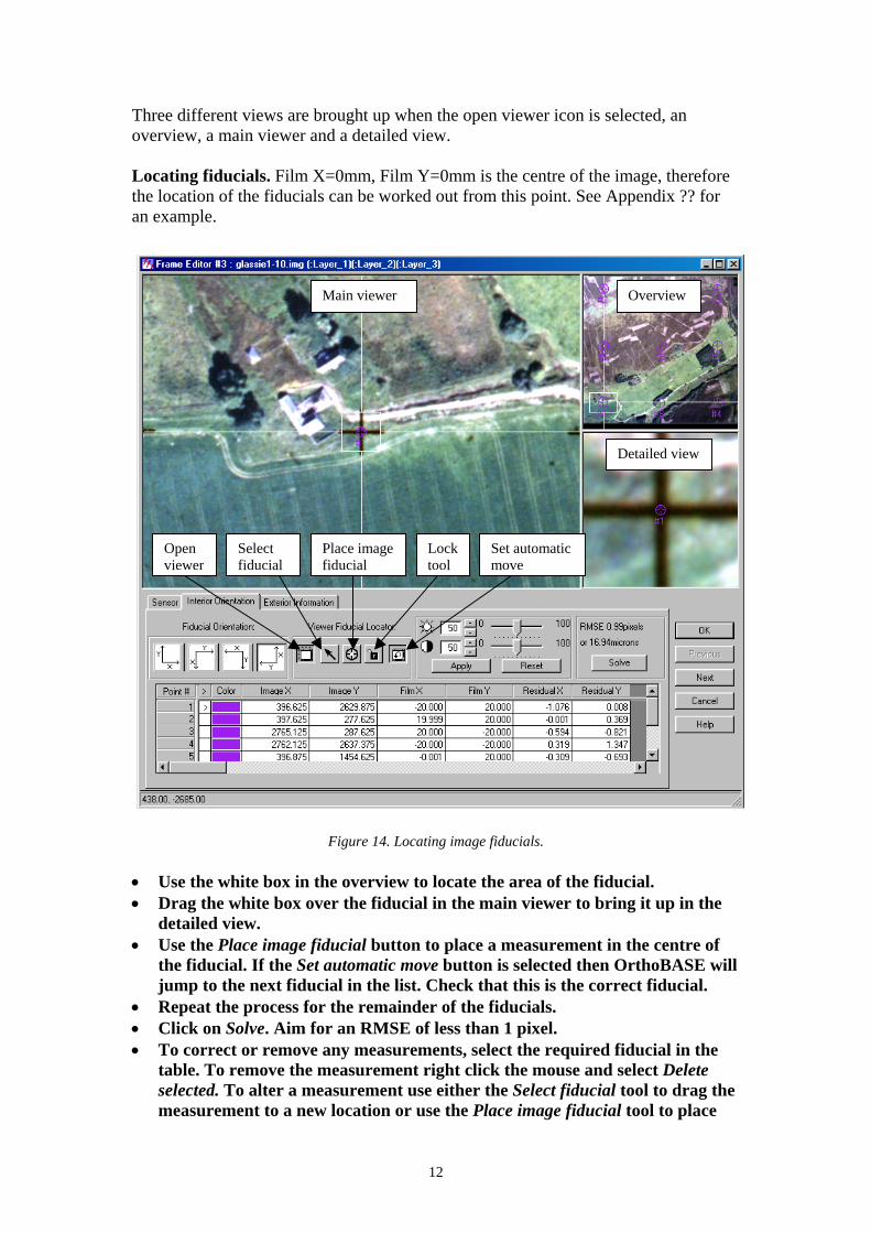
Three different views are brought up when the open viewer icon is selected, an overview, a main viewer and a detailed view. Locating fiducials. Film X=0mm, Film Y=0mm is the centre of the image, therefore the location of the fiducials can be worked out from this point. See Appendix ?? for an example.

Open viewer

Select fiducial

Place image fiducial

Lock tool

Set automatic move

Detailed view

Main viewer Overview

Figure 14. Locating image fiducials. • Use the white box in the overview to locate the area of the fiducial. • Drag the white box over the fiducial in the main viewer to bring it up in the

detailed view. • Use the Place image fiducial button to place a measurement in the centre of

the fiducial. If the Set automatic move button is selected then OrthoBASE will jump to the next fiducial in the list. Check that this is the correct fiducial.

• Repeat the process for the remainder of the fiducials. • Click on Solve. Aim for an RMSE of less than 1 pixel. • To correct or remove any measurements, select the required fiducial in the

table. To remove the measurement right click the mouse and select Delete selected. To alter a measurement use either the Select fiducial tool to drag the measurement to a new location or use the Place image fiducial tool to place

12

the measurement again. Ensure that the correct fiducial is selected in the table.

• Click Next to repeat the process for other images. • Once all images have been completed select the Exterior Information tab. Step 8. Exterior Information • Select the Exterior Orientation tab within the Frame Editor. Enter any known

information.

Figure 15. Specifying exterior orientation information.

• The quality of the information given needs to be specified in the Status row.

Fixed. If the values available are accurate select Fixed. The values will not be altered during triangulation.

Initial. If the values available are an approximation select Initial. The values will be modified during triangulation.

Unknown. If no information about the exterior orientation parameters of the camera is available then select Unknown. OrthoBASE will calculate initial approximations.

Step 9. Ground Point Measurement The purpose of this part of the process is to attach map coordinates and height information to the images by selecting points which are common to two or more images in the block. • Select the Point Measurement button in the main OrthoBASE dialog box. Ground control points can either be Full (X, Y and Z values), Horizontal (X and Y values) or Vertical (Z values only). GCPs can be obtained from theodolite survey, GPS data, planimetric and topographic maps, digital orthorectified images and digital elevation models.

13

Minimum number of GCPs. Theoretically, the minimum number of GCPs is three, two full (X, Y and Z) and one vertical (Z only). It is recommended that for a strip of images there are two GCPs for every third image. It also increases the accuracy of the triangulation if there are three GCPs at the corner edges of the strip. Overview Main view Detailed view

Figure 16. Point measurement tool. Select point. This is the default tool. Create point. Points can be placed in either the main view or the detailed view. Keep current tool. Select this to keep the tool being used, stops the tool being defaulted back to the select point tool.

Reset screen. Undo point measurement. Click to undo edits made, multiple edits can be undone.

Perform automatic tie generation.

14

Automatic tie properties. Perform triangulation. Triangulation properties. Report triangulation results. Set automatic (x, y) drive. This tool automatically moves the viewing area in the right viewer to the approximate location of the point being measured in the left viewer. For this tool to work 3 GCPs in the overlap of the two images have to have already been measured. Clicking on this tool locks it, to unlock click on it again.

Update Z values on selected points. For points selected the Z value will be updated using the vertical reference source specified, e.g. DEM.

Set automatic Z value updating. Clicking on this tool locks the Z value updating function. Therefore for every X and Y coordinates the Z value will be obtained automatically from the vertical reference source specified.

Select points which are common to both left and right viewers. Highlights points in the table which are common to both viewers. Reset horizontal reference source. Click to select the source of X and Y coordinates. Reset vertical reference source. Click to select the source of Z values.

Viewing properties. Click to change the viewing properties of the block.

Show graphic. Click to open the OrthoBASE Graphic Status Display. The OrthoBASE graphic display shows graphically the arrangement of the images, tiepoints and ground control points. It is useful in showing the distribution of tiepoints and ground control points.

15

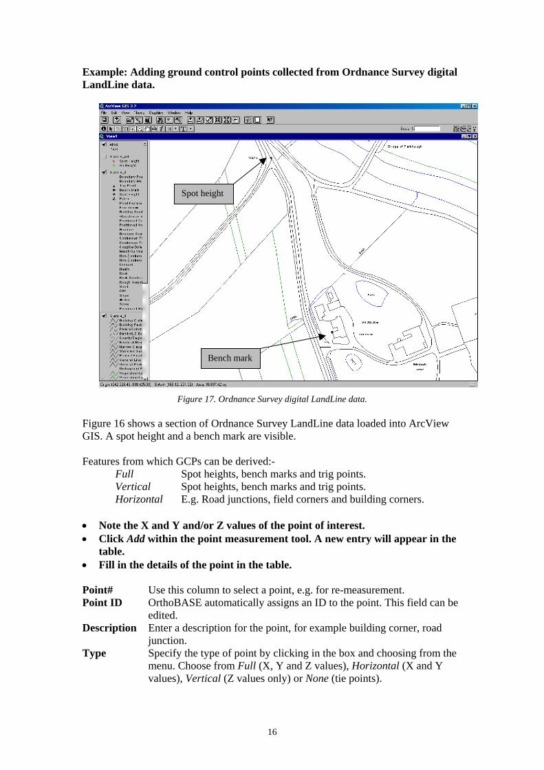
Example: Adding ground control points collected from Ordnance Survey digital LandLine data.

Spot height

Bench mark

Figure 17. Ordnance Survey digital LandLine data. Figure 16 shows a section of Ordnance Survey LandLine data loaded into ArcView GIS. A spot height and a bench mark are visible. Features from which GCPs can be derived:- Full Spot heights, bench marks and trig points. Vertical Spot heights, bench marks and trig points. Horizontal E.g. Road junctions, field corners and building corners. • Note the X and Y and/or Z values of the point of interest. • Click Add within the point measurement tool. A new entry will appear in the

table. • Fill in the details of the point in the table. Point# Use this column to select a point, e.g. for re-measurement. Point ID OrthoBASE automatically assigns an ID to the point. This field can be

edited. Description Enter a description for the point, for example building corner, road

junction. Type Specify the type of point by clicking in the box and choosing from the

menu. Choose from Full (X, Y and Z values), Horizontal (X and Y values), Vertical (Z values only) or None (tie points).

16

Usage Specify either Tie (no values associated with the point), Control (points with X, Y and/or Z values that are to be used in triangulation) or Check (points with X, Y and/or Z values that are to used as comparisons when triangulation is run).

Active X in the relevant box indicates that the point will be used e.g. in triangulation.

X Reference Input the X coordinate (in metres) of the point if it is known. Y Reference Input the Y coordinate (in metres) of the point if it is known. Z Reference Input the Z coordinate (in metres) of the point if it is known. • Select the create point tool and place the point in the two images. • Repeat for other GCPs. • To remove a point, make it inactive by removing the X from the Active

column. Removing suspicious points and running triangulation, enables the user to see what effect the point(s) has on the triangulation results.

• To alter a point, select the required point then either retake the measurement using the create point tool or move the measurement using the select point tool.

Step 10. Automatic Tie Point Measurement Tie points are points which are visible on more than one image but they do not have X, Y or Z values associated with them. Block triangulation usually requires a minimum of nine tie points in each image. The process can be run either from the main OrthoBASE dialog box or from the point measurement tool. • Specify the properties of automatic tie point measurement. From the main

OrthoBASE panel select Edit then Auto. tie point generation properties. From the point measurement tool select the Automatic tie properties button.

17

Figure 18. Automatic tie point generation properties.

• Select Active images only and Tie Points. By selecting Active images only, automatic tie point generation will be performed only on those images marked (X) as active in the main OrthoBASE panel. If there are a lot of images in the block OrthoBASE may return an error due to a lack of memory. If this occurs, perform automatic tie point generation on a few images at a time by making some images inactive in the main OrthoBASE panel. • Specify the required number of tie points per image. • Click OK. • Select the Perform Automatic Tie Generation button from either the main

OrthoBASE panel or the Point Measurement tool. Step 11. Triangulation Once all the points have been entered, triangulation can be run. • Select the Perform Triangulation button from either the main OrthoBASE

panel or the Point Measurement tool.

18

Figure 19. Triangulation summary.

During triangulation OrthoBASE estimates the exterior parameters of the images and the X, Y and Z values of the tie points. These values are then used to compute new image coordinate values. The new image coordinate values are then subtracted from the original image coordinate values. The differences are referred to as the x and y image coordinate residuals. Triangulation is an iterative process and computes new image coordinate values after each iteration. The coordinates from the latest iteration are subtracted from the coordinates from the previous iteration. If these differences are greater than the convergence value the iterations continue. • Check that Triangulation Iteration Convergence = Yes. • Check the Total Image Unit-Weight RMSE. • Check the Control Point RMSEs. Figures in brackets refer to the number of

points contributing, e.g. in the example above 39 points have X values. • For more detailed results click Report. For a more detailed description of the triangulation report see the online help. • If the Triangulation Iteration Convergence = No

or high RMSEs (greater than 5) are obtained check the following: • There are enough ground control points (Minimum – 2 full and 1 vertical per

block but more than this is usually required) and tie points (Minimum – 9 per image).

• Typing errors (X, Y and Z reference). • Points placed in the wrong area. • Within the triangulation report check the residuals of the control points. Look

for high positive or negative values. Try inactivating these points and re-running triangulation to see what effect they have on the results.

19

•

Uppo

The residuals of the control points Point ID rX rY rZ 3 1.5009 3.0214 2.1724 4 0.9184 -0.4119 -6.1148 5 -0.2294 0.0139 0.5685 6 -0.7518 -0.4529 2.3241 27 0.5421 0.3611 5.5348 29 1.5567 0.2313 0.4284 10 -1.1486 0.0405 11 -1.3804 1.8145 12 1.0760 -2.1970 13 -2.2279 -0.4136 14 -0.1003 1.8349 15 1.4946 -2.5647 16 -1.6088 -2.0725 17 0.5586 0.3197 18 -0.8044 -0.8017 19 -1.0555 0.0520 20 -1.2832 -0.1049 21 0.4822 -1.0359 22 0.1771 1.3830 24 1.0989 0.4080 25 -0.6125 2.6665 26 3.7632 1.6007 9 0.4502 -0.1863 30 -1.8242 -0.2195 158 1.3736 4.2147 279 -0.6746 2.1913 931 0.3333 1.8131

932 3.4308 1.8884

Figure 20. Control point residual section of the triangulation report.

Once acceptable triangulation results have been obtained, click Update and Accept.

date and accepting the triangulation results attributes X, Y and Z values to both tie ints and to ground control points with missing information.

20

Step 12. Orthoresampling • Select the Orthoresampling button from the main OrthoBASE panel. • Ensure that all images to be orthorectified are active in the main OrthoBASE

panel.

Figure 21. Defining orthoresampling properties.

• To orthorectify multiple files, select Multiple File Output and specify a prefix

to be added to the beginning of the original image file name. • Select DEM File and specify the DEM to be used. • For the resample method choose one of the following:-

Bilinear Interpolation. Use this method if the resolution of the DEM is greater than the resolution of the image or if the output area of the orthorectified image is covered entirely by the DEM. Nearest Neighbour. Use this method if the resolution of the DEM and the image is approximately the same or if the output orthorectified image is not covered entirely by the DEM.

21

• Enter the required output cell sizes. For example, entering 1 in the X and Y fields would produce a 1m orthorectified image.

• Click OK to begin the orthorectification process.

Figure 22. Orthoresampling process monitor.

• Click OK once the Job State is Done for all the images selected for

orthoresampling.

22

Appendix I Example Frame Imagery

LCS88 Aerial Photography Scale 1:24000 Camera. Wild RC20 (for more information see Appendix III.) Fiducials Marked by purple circles Scanned 256 level grey 400 dpi

Figure 23. LCS88 aerial photography.

23

Colour frame photography Scale. 1:5000 Camera. Rolleiflex 6006 (for more information see Appendix III.) Fiducials. Marked by purple circles Scanned. 24 bit colour 600 dpi

Figure 24. Colour frame photography.

24

Appendix II Other Types of Imagery

Videography

Figure 25. Infra red videography.

Figure 23 shows 1:5000 infra red videography. The imagery was captured using a video camera, individual frames of the imagery were then captured to be orthorectified. This type of imagery can also be orthorectified within OrthoBASE. • Follow the procedure laid out for frame photography with the following

exceptions. Step 2. Select geometric model • Select Video Camera (Videography) and click OK. Step 6. Defining the sensor The same information is required under the sensor tab as was for the frame camera. It is however advantageous to have as much information as possible as a video camera is not as accurate as a photogrammetric camera. Specification for video camera used to capture Figure 23 IR videography Focal Length (mm) 8.54 Principal Point xo (mm) 0.00 Principal Point yo (mm) 0.00

Radial Lens Distortion Radial Dist Distortion (microns) Residual (microns) 0 0 0 1.74 -17.44 0.98 2.79 -54.78 -1.85 3.50 -105.12 1.37 4.23 -169.04 -0.32

25

Step 7. Interior Orientation Video cameras are non-metric cameras, therefore they do not have fiducial marks. Instead the pixel size of the imagery must be defined. • Define the Pixel size in x direction (microns). • Define the Pixel size in y direction (microns). For example, for the imagery in Figure 23: Pixel size in x direction (microns) = 11.4583 Pixel size in y direction (microns) = 11.4583

26

Appendix III Sensor Specifications

Wild RC20 Camera Name Wild RC20 Focal Length (mm) 153.23 Principal Point xo (mm) 0.00 Principal Point yo (mm) 0.00 Fiducials

Film X (mm) Film Y (mm) 1 106.004 -106.008 2 -105.999 -105.998 3 -106.004 106.005 4 106.002 106.002 5 0.003 -109.992 6 -109.996 0.003 7 -0.004 109.997 8 109.998 -0.002

Rolleiflex 6006 Camera Name Rolleiflex 6006 Focal Length(mm) 80.11 Principal Point xo (mm) 0.1300 Principal Point yo (mm) 0.2900 Fiducials

Film X (mm) Film Y (mm) 1 -24.999 25.000 2 25.000 25.000 3 25.000 -25.000 4 -24.999 -25.000 5 0.000 24.999 6 25.001 0.001 7 -0.002 -24.999 8 -25.000 0.002 9 0.000 0.000

27

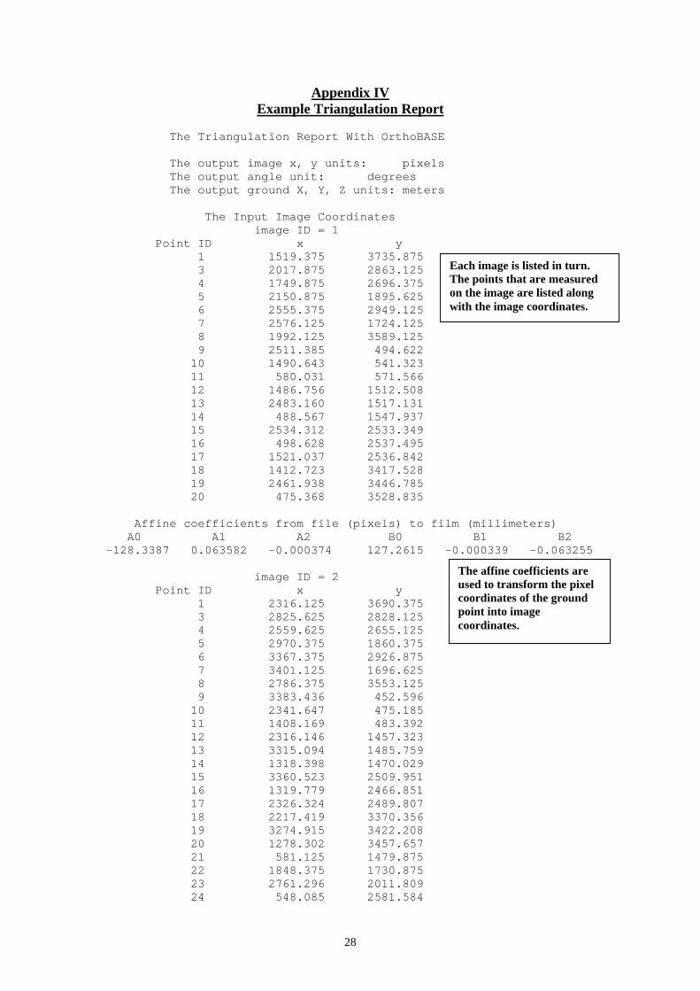
Appendix IV Example Triangulation Report

The Triangulation Report With OrthoBASE The output image x, y units: pixels The output angle unit: degrees The output ground X, Y, Z units: meters The Input Image Coordinates image ID = 1 Point ID x y 1 1519.375 3735.875

Each image is listed in turn. The points that are measured on the image are listed along with the image coordinates.

3 2017.875 2863.125 4 1749.875 2696.375 5 2150.875 1895.625 6 2555.375 2949.125 7 2576.125 1724.125 8 1992.125 3589.125 9 2511.385 494.622 10 1490.643 541.323 11 580.031 571.566 12 1486.756 1512.508 13 2483.160 1517.131 14 488.567 1547.937 15 2534.312 2533.349 16 498.628 2537.495 17 1521.037 2536.842 18 1412.723 3417.528 19 2461.938 3446.785 20 475.368 3528.835 Affine coefficients from file (pixels) to film (millimeters) A0 A1 A2 B0 B1 B2 -128.3387 0.063582 -0.000374 127.2615 -0.000339 -0.063255

The affine coefficients are used to transform the pixel coordinates of the ground point into image coordinates.

image ID = 2 Point ID x y 1 2316.125 3690.375 3 2825.625 2828.125 4 2559.625 2655.125 5 2970.375 1860.375 6 3367.375 2926.875 7 3401.125 1696.625 8 2786.375 3553.125 9 3383.436 452.596 10 2341.647 475.185 11 1408.169 483.392 12 2316.146 1457.323 13 3315.094 1485.759 14 1318.398 1470.029 15 3360.523 2509.951 16 1319.779 2466.851 17 2326.324 2489.807 18 2217.419 3370.356 19 3274.915 3422.208 20 1278.302 3457.657 21 581.125 1479.875 22 1848.375 1730.875 23 2761.296 2011.809 24 548.085 2581.584

28

25 922.335 2212.276 26 530.057 2961.144 27 1219.973 3045.746 28 402.998 369.852 29 2040.063 379.362 30 1123.948 447.625 31 2608.514 525.128 32 429.693 1163.743 33 2642.365 1207.550 34 1185.392 1216.432 35 2007.685 1235.668 36 2759.129 1961.019 37 2024.367 1995.693 38 1161.097 2001.059 39 404.770 2025.434 40 2038.031 2783.690 41 1213.844 2800.919 42 2694.310 2811.848 43 533.431 2956.053 44 554.658 3249.249 45 766.157 3253.502 46 794.266 3349.697 47 2714.570 3389.352 48 642.909 3445.632 49 771.367 3518.452 50 1987.620 3554.483 51 1147.312 3631.226 52 2727.112 2109.896 Affine coefficients from file (pixels) to film (millimeters) A0 A1 A2 B0 B1 B2 -131.1987 0.063598 -0.000203 125.0123 -0.000168 -0.063261 image ID = 3 Point ID x y 1 3487.125 3576.875 21 1688.625 1395.125 4 3710.125 2544.625 22 2969.579 1624.780 23 3895.776 1891.254 24 1687.033 2505.576 25 2049.056 2129.017 26 1674.988 2883.038 27 2382.730 2957.153 28 1479.184 262.471 29 3153.133 229.731 30 2192.395 324.876 31 3749.911 365.782 32 1529.890 1077.680 33 3778.048 1071.728 34 2300.920 1112.802 35 3138.907 1115.336 36 3894.313 1839.839 37 3152.391 1889.795 38 2290.598 1912.302 39 1531.441 1950.592 40 3179.979 2682.001 41 2371.848 2712.822 42 3849.422 2699.346 43 1677.346 2877.475 44 1718.383 3166.124

29

45 1935.166 3167.900 46 1968.528 3262.204 47 3869.313 3274.031 48 1819.690 3357.986 49 1953.303 3428.188 50 3171.006 3447.520 51 2325.657 3534.249 52 3862.596 1991.580 54 950.320 1529.529 56 1970.016 351.930 57 1198.052 381.646 58 2785.460 438.956 59 407.279 507.958 60 736.714 1015.833 61 2806.325 1239.786 62 1986.540 1251.261 63 651.009 1259.179 64 1195.727 1263.751 65 740.093 1265.549 66 695.008 1330.306 67 627.911 1515.862 68 444.699 1976.114 69 2009.817 1994.295 70 1182.185 2018.766 71 2768.181 2018.731 72 445.869 2826.782 73 2731.172 2836.017 74 1192.926 2845.641 75 2043.463 2839.681 76 740.377 3251.097 77 746.921 3296.048 78 2620.695 3566.379 79 1999.469 3598.292 80 1268.781 3639.271 81 564.934 177.723 82 878.158 292.419 83 1988.798 296.642 84 596.573 293.020 85 2621.168 301.607 86 1127.567 396.675 87 1032.307 405.548 88 487.770 517.570 89 529.253 537.197 90 461.398 545.431 91 543.933 541.369 92 434.423 591.931 93 609.415 629.481 94 467.313 692.560 95 826.853 777.163 96 2525.125 815.364 97 1932.877 818.987 98 1436.859 844.336 99 877.506 1094.035 100 1415.229 1380.453 101 2546.705 1397.535 102 2027.489 1462.111 103 862.693 1567.987 104 554.788 1699.258 105 925.670 1997.269 106 1417.955 2001.802 107 2589.251 2065.677

30

108 2585.311 2603.196 109 383.142 2601.695 110 1485.410 2618.182 111 2039.492 2617.191 112 823.248 2624.725 113 560.599 2917.842 114 2041.010 3110.576 115 2598.733 3152.113 116 1374.081 3176.414 117 923.621 3229.651 118 1052.297 3649.770 119 1413.728 3696.801 120 2006.314 3714.035 121 2496.813 3712.573 122 1400.727 2935.548 124 484.023 1110.637 125 1675.624 1313.618 126 1155.456 1262.765 Affine coefficients from file (pixels) to film (millimeters) A0 A1 A2 B0 B1 B2 -134.4256 0.063583 -0.000457 123.1679 -0.000410 -0.063259 image ID = 4 Point ID x y 21 2714.625 1447.875 24 2741.284 2570.579 25 3093.310 2178.728 26 2733.807 2953.071 27 3471.448 3009.038 54 1945.446 1605.175 56 2954.894 382.170 57 2203.456 436.012 58 3794.023 443.012 59 1367.739 591.820 60 1730.330 1093.138 61 3847.705 1255.256 62 3018.958 1291.871 63 1626.225 1343.227 64 2193.763 1328.993 65 1721.658 1345.525 66 1675.149 1412.227 67 1609.567 1601.820 68 1451.438 2072.119 69 3058.778 2044.424 70 2224.109 2092.915 71 3822.536 2047.016 72 1515.230 2929.581 73 3815.405 2877.454 74 2249.398 2930.269 75 3115.156 2899.363 76 1829.237 3350.678 77 1837.242 3396.225 78 3729.312 3620.489 79 3102.915 3668.553 80 2352.600 3729.692 81 1516.909 252.189 82 1872.681 356.663 83 2976.570 325.079 84 1566.114 367.004 85 3622.005 308.915

31

86 2132.343 453.591 87 2036.190 465.760 88 1459.187 598.057 89 1505.166 616.651 90 1429.604 627.344 91 1521.620 620.300 92 1405.434 675.389 93 1593.505 707.550 94 1444.915 776.140 95 1834.586 847.835 96 3553.498 833.349 97 2946.684 856.037 98 2451.043 896.427 99 1873.054 1167.083 100 2421.947 1440.975 101 3593.627 1422.378 102 3073.686 1503.911 103 1856.880 1646.675 104 1543.070 1789.143 105 1965.610 2078.356 106 2458.085 2069.381 107 3641.797 2099.557 108 3672.044 2645.027 109 1442.684 2704.491 110 2541.379 2690.802 111 3091.192 2674.412 112 1877.064 2717.197 113 1628.035 3018.860 114 3124.859 3173.870 115 3691.971 3200.909 116 2446.617 3260.231 117 2011.848 3324.994 118 2135.066 3745.477 119 2509.169 3784.516 120 3115.706 3785.998 121 3610.636 3772.144 122 2462.954 3014.736 124 1460.128 1198.539 125 2700.083 1365.607 126 2154.105 1328.711 Affine coefficients from file (pixels) to film (millimeters) A0 A1 A2 B0 B1 B2 -134.3869 0.063586 0.000013 127.0052 0.000045 -0.063262

32

THE OUTPUT OF SELF-CALIBRATING BUNDLE BLOCK ADJUSTMENT the no. of iteration =1 the standard error = 1.0287 the maximal correction of the object points = 176.46666 the no. of iteration =2 the standard error = 1.0174 the maximal correction of the object points = 2.03745 the no. of iteration =3 the standard error = 1.0176 the maximal correction of the object points = 0.00604 the no. of iteration =4 the standard error = 1.0176 the maximal correction of the object points = 0.00002

The calculations are redone until the maximal correction of the object points is less than 0.001 (the convergence value). In this example it has taken four iterations. The standard error is a global indicator of quality.

The exterior orientation parameters image ID Xs Ys Zs OMEGA PHI KAPPA 1 342626.1828 839279.9113 4174.6864 1.6073 1.1402 1.6777 2 341340.1026 839232.2968 4171.6558 1.2362 1.0662 2.8898 3 339632.8642 839152.6748 4166.9242 0.0168 1.4430 2.0738 4 337959.6896 839105.1744 4164.6899 -0.0100 1.7130 0.0143

Estimated exterior orientation parameters. The interior orientation parameters of photos

The interior orientation parameters (focal length and principal point) remain as inputed.

image ID f(mm) xo(mm) yo(mm) 1 152.2400 0.0000 0.0000 2 152.2400 0.0000 0.0000 3 152.2400 0.0000 0.0000 4 152.2400 0.0000 0.0000 The residuals of the control points Point ID rX rY rZ 1 2.4358 -0.6450 -0.7271 3 0.1541 0.6455 -1.6778 6 0.8140 0.8453 -0.9678 7 1.0846 1.6680 2.5452 21 3.0184 -2.3048 0.3643 23 0.6543 -0.1429 -3.3105 54 -2.0225 2.4939 -1.3090 125 1.4557 -1.4018 0.8862 126 -1.4303 0.4299 1.4235 5 -1.7202 0.2516

In the process new control coordinates are calculated. Controlpoint residuals represent the difference between the original control point coordinates and the estimated control point coordinates.

24 0.2169 4.1949 25 1.9107 -2.0056 26 4.4972 3.5971 27 -3.4050 -4.1109 8 -2.5899 3.8657 122 -1.3011 -1.9714 124 -6.6115 4.4751 4 -0.6436 -2.1176 22 -2.9674 -0.3853

33

aX aY aZ -0.3395 0.3885 -0.3081 mX mY mZ 2.5690 2.4392 1.7119

aX, aY and aZ are the average residuals for the control point coordinates. mX, mY and mZ are the root mean square errors (standard deviation).

All the control points are listed X, Y and Z values. Those values that were inputed remain the same, those that were unknown have been estimated. Tie points are also listed with estimated X, Y and Z values.

The coordinates of object points Point ID X Y Z Overlap 1 341791.2000 836594.5000 265.1200 3 3 342560.8000 837989.9000 231.4100 2 6 343435.3000 837880.2000 233.7800 2 7 343443.3000 839871.3000 184.4000 2 21 338799.6800 839997.7200 324.4000 3 23 342412.3000 839306.6000 194.8000 2 54 337570.5000 839758.0100 261.1100 2 125 338777.2000 840125.7000 329.3100 2 126 337911.2000 840199.7000 284.4200 2 5 342745.0000 839569.9000 200.6021 2 24 338848.9000 838208.0000 310.1316 3 25 339412.9000 838836.7000 285.7046 3 26 338838.2000 837591.4000 287.4224 3 27 339994.2000 837540.9000 323.1814 3 8 342549.6000 836823.9000 222.7657 2 122 338406.7100 837506.8000 319.9132 2 124 336777.3000 840423.3000 269.4953 2 4 342117.3000 838250.0000 237.0913 3 22 340888.2000 839692.4000 248.7536 2 9 343277.6484 841859.4845 314.8575 2 10 341597.8564 841772.6725 297.3594 2 11 340050.5223 841724.8943 262.4435 2 12 341631.6416 840171.3005 263.0642 2 13 343280.1413 840209.5177 209.1129 2 14 340016.4360 840062.5263 338.6576 2 15 343383.4914 838553.3286 266.9977 2 16 340111.0604 838470.4468 354.3184 2 17 341728.4186 838491.0214 217.6815 2 18 341611.0267 837100.2609 284.9889 2 19 343291.2595 837114.3803 283.7301 2 20 340121.0220 836897.8034 325.7788 2 28 338420.1955 841786.7168 360.9048 2 29 341096.2969 841911.9184 300.0207 2 30 339563.4723 841777.5236 246.1940 2 31 342034.0447 841698.9383 311.7661 2 32 338535.7842 840493.5947 346.1251 2 33 342148.5852 840609.7671 250.7049 2 34 339774.9140 840465.9633 333.8041 2 35 341111.4342 840499.8223 306.8290 2 36 342404.5171 839389.5336 196.8402 2 37 341195.1160 839273.0991 238.2453 2 38 339796.2467 839195.5580 308.0531 2 39 338576.6643 839097.6027 337.0819 2 40 341278.7432 837994.0872 231.4867 2

34

41 339961.7577 837926.5571 330.1923 2 42 342346.6528 838006.9591 233.6315 2 43 338844.8914 837601.5634 282.6550 2 44 338932.6154 837155.9872 320.6671 2 45 339284.3223 837176.7346 336.3683 2 46 339342.8378 837033.2358 344.4289 2 47 342426.3358 837070.3893 202.2192 2 48 339108.7214 836869.9336 344.6673 2 49 339326.9141 836774.1674 354.0642 2 50 341258.2682 836816.3593 329.1610 2 51 339926.2245 836615.0871 325.4701 2 52 342362.8424 839142.4001 193.7755 2 56 339201.3447 841718.8123 260.3811 2 57 337988.0975 841563.5143 400.3786 2 58 340531.7162 841599.0342 255.9053 2 59 336621.7545 841412.5567 282.7002 2 60 337227.4033 840572.1924 327.3468 2 61 340594.4874 840296.2219 288.3053 2 62 339278.0386 840234.3491 336.9249 2 63 337037.4451 840198.3334 236.6882 2 64 337973.9828 840201.2289 279.9879 2 65 337199.2632 840187.6530 253.8924 2 66 337120.4959 840081.3385 244.5887 2 67 337009.4474 839772.8627 234.5391 2 68 336764.2164 839001.1613 293.1212 2 69 339348.2960 839050.2549 316.4418 2 70 338022.3420 838972.2317 361.6277 2 71 340576.7859 839046.8388 257.4300 2 72 336908.7223 837663.7960 431.7828 2 73 340548.8524 837735.5405 283.6632 2 74 338063.9840 837637.9188 325.8858 2 75 339441.3191 837695.4615 306.5804 2 76 337405.0049 837016.3757 435.3028 2 77 337417.6049 836945.9685 435.3216 2 78 340400.9542 836573.2488 306.5536 2 79 339407.9175 836502.7540 345.5154 2 80 338228.7950 836373.5614 335.0779 2 81 336865.7424 841964.9867 275.6276 2 82 337466.0840 841700.5622 396.5903 2 83 339231.0484 841799.2354 275.3517 2 84 336960.3360 841741.1901 326.9904 2 85 340259.2249 841815.1814 259.6281 2 86 337876.4076 841536.8662 402.3644 2 87 337725.3102 841518.3718 405.9542 2 88 336783.4203 841379.0132 317.4522 2 89 336861.8626 841341.2563 329.0470 2 90 336730.8281 841340.3687 304.1703 2 91 336890.0670 841331.9834 334.1287 2 92 336693.5915 841259.3252 311.5737 2 93 337009.1286 841185.5819 343.3830 2 94 336761.8691 841090.0030 322.8795 2 95 337406.1537 840928.9058 397.3077 2 96 340120.7144 840955.1138 315.0657 2 97 339169.7680 840929.7158 320.2149 2 98 338380.0269 840855.4248 363.5971 2 99 337456.6245 840455.1218 315.1781 2 100 338342.7107 840018.6948 280.8939 2 101 340181.3691 840027.2710 318.7995 2 102 339355.2141 839895.3317 360.2644 2 103 337423.0483 839693.6117 258.9381 2 104 336901.6806 839464.1123 245.0537 2

35

105 337612.6188 838994.7290 377.3896 2 106 338394.9909 839009.7109 337.0540 2 107 340288.9055 838962.7052 264.6306 2 108 340295.9296 838113.1281 331.7469 2 109 336791.3261 838012.9249 424.6848 2 110 338529.4737 838022.2080 323.5499 2 111 339421.8823 838038.0564 257.2479 2 112 337471.1102 837984.4875 369.2134 2 113 337081.4811 837516.4875 407.2074 2 114 339450.7222 837268.3825 322.2554 2 115 340348.7171 837227.2685 296.8019 2 116 338377.9917 837121.9704 334.1617 2 117 337690.0706 837054.2787 421.3042 2 118 337881.9054 836349.5796 347.8596 2 119 338474.3308 836310.0104 358.8189 2 120 339424.6659 836325.5058 354.0198 2 121 340207.5518 836342.2192 322.5158 2 The total object points = 122 The residuals of image points The residuals of image

points represent the difference between the original image coordinates and the estimated image coordinates. High values can be a good indication of inaccurate placement of points.

Point Image Vx Vy 1 1 -1.565 0.519 1 2 -1.519 -0.361 1 3 -1.251 -0.676 Point Image Vx Vy 3 1 -0.131 0.490 3 2 0.192 0.992 Point Image Vx Vy 6 1 -0.396 0.445 6 2 -0.218 1.014 Point Image Vx Vy 7 1 -0.998 0.731 7 2 -1.529 1.664 Point Image Vx Vy 21 2 -1.709 -1.313 21 3 -1.548 -1.085 21 4 -2.085 -1.854 Point Image Vx Vy 23 2 0.149 -0.886 23 3 1.057 0.621 Point Image Vx Vy 54 3 0.752 0.886 54 4 1.171 1.915 Point Image Vx Vy 125 3 -0.753 -0.392 125 4 -1.053 -1.085 Point Image Vx Vy 126 3 1.225 -0.113 126 4 0.918 1.142 Point Image Vx Vy 5 1 1.035 0.332

36

5 2 1.044 0.048 Point Image Vx Vy 24 2 -0.412 2.729 24 3 0.033 2.118 24 4 -0.249 2.987 Point Image Vx Vy 25 2 -0.695 -1.605 25 3 -1.911 -1.688 25 4 -0.805 -0.552 Point Image Vx Vy 26 2 -3.001 2.203 26 3 -2.536 1.641 26 4 -2.947 2.558 Point Image Vx Vy 27 2 2.283 -1.512 27 3 2.109 -3.120 27 4 2.232 -2.935 Point Image Vx Vy 8 1 1.538 2.112 8 2 1.501 2.917 Point Image Vx Vy 122 3 0.831 -1.043 122 4 0.815 -1.374 Point Image Vx Vy 124 3 3.843 3.401 124 4 3.971 2.107 Point Image Vx Vy 4 1 0.634 -1.408 4 2 0.093 -1.354 4 3 0.595 -1.139 Point Image Vx Vy 22 2 1.809 -0.323 22 3 1.854 -0.021 Point Image Vx Vy 9 1 -0.008 -0.292 9 2 0.001 0.288 Point Image Vx Vy 10 1 -0.001 -0.033 10 2 0.000 0.033 Point Image Vx Vy 11 1 0.000 0.010 11 2 -0.000 -0.010 Point Image Vx Vy 12 1 -0.005 -0.283 12 2 -0.001 0.280 Point Image Vx Vy 13 1 -0.009 -0.468

37

13 2 -0.002 0.464 Point Image Vx Vy 14 1 0.005 0.273 14 2 0.002 -0.270 Point Image Vx Vy 15 1 -0.002 -0.211 15 2 -0.003 0.210 Point Image Vx Vy 16 1 0.002 0.258 16 2 0.004 -0.257 Point Image Vx Vy 17 1 0.001 0.097 17 2 0.001 -0.097 Point Image Vx Vy 18 1 -0.000 0.521 18 2 0.012 -0.521 Point Image Vx Vy 19 1 -0.001 -0.422 19 2 -0.009 0.423 Point Image Vx Vy 20 1 -0.001 -0.584 20 2 -0.012 0.584 Point Image Vx Vy 28 2 0.012 1.098 28 3 -0.037 -1.059 Point Image Vx Vy 29 2 -0.003 -0.259 29 3 0.009 0.249 Point Image Vx Vy 30 2 0.003 0.295 30 3 -0.010 -0.285 Point Image Vx Vy 31 2 -0.014 -1.044 31 3 0.037 1.003 Point Image Vx Vy 32 2 0.003 0.685 32 3 -0.018 -0.670 Point Image Vx Vy 33 2 -0.007 -0.924 33 3 0.026 0.899 Point Image Vx Vy 34 2 -0.004 -0.521 34 3 0.014 0.509 Point Image Vx Vy 35 2 -0.002 -0.280 35 3 0.007 0.273

38

Point Image Vx Vy 36 2 -0.001 -0.719 36 3 0.014 0.708 Point Image Vx Vy 37 2 0.000 -0.244 37 3 0.004 0.241 Point Image Vx Vy 38 2 -0.000 0.275 38 3 -0.005 -0.272 Point Image Vx Vy 39 2 -0.000 0.090 39 3 -0.002 -0.089 Point Image Vx Vy 40 2 0.000 -0.048 40 3 0.000 0.048 Point Image Vx Vy 41 2 -0.002 0.192 41 3 -0.002 -0.193 Point Image Vx Vy 42 2 0.001 -0.094 42 3 0.001 0.094 Point Image Vx Vy 43 2 -0.001 0.055 43 3 -0.000 -0.056 Point Image Vx Vy 44 2 0.003 -0.280 44 3 0.001 0.284 Point Image Vx Vy 45 2 -0.001 0.061 45 3 -0.000 -0.062 Point Image Vx Vy 46 2 -0.000 0.015 46 3 -0.000 -0.015 Point Image Vx Vy 47 2 -0.001 0.054 47 3 -0.000 -0.055 Point Image Vx Vy 48 2 0.004 -0.351 48 3 0.001 0.357 Point Image Vx Vy 49 2 0.002 -0.127 49 3 0.000 0.130 Point Image Vx Vy 50 2 -0.002 0.161 50 3 0.000 -0.163

39

Point Image Vx Vy 51 2 -0.002 0.107 51 3 0.000 -0.109 Point Image Vx Vy 52 2 0.000 -0.616 52 3 0.011 0.608 Point Image Vx Vy 56 3 0.000 0.007 56 4 -0.000 -0.007 Point Image Vx Vy 57 3 0.001 0.056 57 4 -0.003 -0.055 Point Image Vx Vy 58 3 -0.004 -0.242 58 4 0.011 0.238 Point Image Vx Vy 59 3 0.006 0.400 59 4 -0.018 -0.396 Point Image Vx Vy 60 3 0.001 0.054 60 4 -0.002 -0.054 Point Image Vx Vy 61 3 0.000 0.008 61 4 -0.000 -0.008 Point Image Vx Vy 62 3 -0.000 -0.060 62 4 0.002 0.059 Point Image Vx Vy 63 3 0.002 0.378 63 4 -0.013 -0.374 Point Image Vx Vy 64 3 -0.003 -0.402 64 4 0.015 0.397 Point Image Vx Vy 65 3 -0.002 -0.231 65 4 0.008 0.228 Point Image Vx Vy 66 3 -0.002 -0.329 66 4 0.012 0.325 Point Image Vx Vy 67 3 -0.001 -0.311 67 4 0.010 0.308 Point Image Vx Vy 68 3 0.000 -0.043 68 4 0.001 0.042

40

Point Image Vx Vy 69 3 -0.000 0.069 69 4 -0.002 -0.068 Point Image Vx Vy 70 3 0.000 -0.106 70 4 0.003 0.105 Point Image Vx Vy 71 3 0.000 -0.025 71 4 0.001 0.024 Point Image Vx Vy 72 3 0.004 -0.366 72 4 0.006 0.362 Point Image Vx Vy 73 3 -0.002 0.215 73 4 -0.003 -0.211 Point Image Vx Vy 74 3 -0.006 0.529 74 4 -0.008 -0.523 Point Image Vx Vy 75 3 0.002 -0.184 75 4 0.003 0.182 Point Image Vx Vy 76 3 0.002 -0.123 76 4 0.001 0.121 Point Image Vx Vy 77 3 -0.000 0.028 77 4 -0.000 -0.028 Point Image Vx Vy 78 3 0.001 -0.058 78 4 0.000 0.057 Point Image Vx Vy 79 3 0.005 -0.281 79 4 0.002 0.277 Point Image Vx Vy 80 3 -0.001 0.054 80 4 -0.000 -0.053 Point Image Vx Vy 81 3 -0.002 -0.084 81 4 0.004 0.083 Point Image Vx Vy 82 3 0.004 0.205 82 4 -0.010 -0.202 Point Image Vx Vy 83 3 -0.002 -0.119 83 4 0.006 0.117 Point Image Vx Vy

41

84 3 -0.001 -0.059 84 4 0.003 0.058 Point Image Vx Vy 85 3 -0.005 -0.301 85 4 0.015 0.296 Point Image Vx Vy 86 3 0.002 0.093 86 4 -0.004 -0.092 Point Image Vx Vy 87 3 0.002 0.145 87 4 -0.007 -0.143 Point Image Vx Vy 88 3 0.003 0.187 88 4 -0.009 -0.185 Point Image Vx Vy 89 3 0.005 0.317 89 4 -0.014 -0.314 Point Image Vx Vy 90 3 0.004 0.250 90 4 -0.011 -0.247 Point Image Vx Vy 91 3 0.004 0.304 91 4 -0.014 -0.301 Point Image Vx Vy 92 3 0.005 0.396 92 4 -0.018 -0.392 Point Image Vx Vy 93 3 0.007 0.533 93 4 -0.023 -0.527 Point Image Vx Vy 94 3 0.007 0.550 94 4 -0.023 -0.544 Point Image Vx Vy 95 3 -0.002 -0.137 95 4 0.006 0.135 Point Image Vx Vy 96 3 0.001 0.069 96 4 -0.003 -0.068 Point Image Vx Vy 97 3 0.001 0.086 97 4 -0.004 -0.085 Point Image Vx Vy 98 3 -0.003 -0.251 98 4 0.011 0.247 Point Image Vx Vy 99 3 -0.003 -0.344

42

99 4 0.013 0.340 Point Image Vx Vy 100 3 -0.000 -0.040 100 4 0.001 0.040 Point Image Vx Vy 101 3 -0.002 -0.349 101 4 0.012 0.344 Point Image Vx Vy 102 3 -0.001 -0.123 102 4 0.004 0.121 Point Image Vx Vy 103 3 -0.002 -0.544 103 4 0.018 0.538 Point Image Vx Vy 104 3 -0.001 -0.310 104 4 0.010 0.306 Point Image Vx Vy 105 3 0.000 -0.232 105 4 0.006 0.229 Point Image Vx Vy 106 3 -0.000 0.088 106 4 -0.002 -0.087 Point Image Vx Vy 107 3 0.000 -0.179 107 4 0.005 0.176 Point Image Vx Vy 108 3 -0.001 0.142 108 4 -0.003 -0.140 Point Image Vx Vy 109 3 0.001 -0.152 109 4 0.003 0.150 Point Image Vx Vy 110 3 0.001 -0.103 110 4 0.002 0.102 Point Image Vx Vy 111 3 0.001 -0.161 111 4 0.003 0.158 Point Image Vx Vy 112 3 -0.006 0.600 112 4 -0.010 -0.594 Point Image Vx Vy 113 3 0.002 -0.183 113 4 0.003 0.182 Point Image Vx Vy 114 3 0.002 -0.124 114 4 0.002 0.122

43

Point Image Vx Vy 115 3 0.002 -0.131 115 4 0.002 0.129 Point Image Vx Vy 116 3 -0.012 0.745 116 4 -0.008 -0.737 Point Image Vx Vy 117 3 -0.005 0.300 117 4 -0.003 -0.297 Point Image Vx Vy 118 3 0.003 -0.153 118 4 0.001 0.151 Point Image Vx Vy 119 3 -0.005 0.265 119 4 -0.001 -0.262 Point Image Vx Vy 120 3 0.001 -0.072 120 4 0.000 0.071 Point Image Vx Vy 121 3 -0.001 0.062 121 4 -0.000 -0.061

44