ephemeris determination using a connected … · 34th annual precise time and time interval (ptti)...

34th Annual Precise Time and Time Interval (PTTI) Meeting

295

EPHEMERIS DETERMINATION USING A CONNECTED ELEMENT INTERFEROMETER

D. Morrison

RINCON Research Corporation

S. Pogorelc Northrop Grumman TASC

T. Celano

Timing Solutions Corporation

A. Gifford National Institute of Standards and Technology

Abstract

This paper describes a connected element interferometer that has been developed and is

operating with collection elements in Tucson and Phoenix with a separation of 180 km. Coherence between the collection sites of better than 50 picoseconds is achieved through two-way time transfer over a commercial fiber optics link. The description of hardware and software implementation, as well as measurement results of several operating satellites, are presented. Consider analysis is also presented to demonstrate the projected system performance against different targets, based on the characteristics of the measurement using the existing Tucson-Phoenix link.

1. INTRODUCTION The application of a Connected Element Interferometer (CEI) for the purpose of satellite ephemeris determination was recently investigated. The method is based on the passive reception of radio frequency (RF) signals. Two interferometer tracking sites, located in Tucson and Phoenix, were connected by optical fiber that provided high-speed data transfer between the sites together with time and frequency synchronization. The resulting measurement was the Time Difference of Arrival (TDOA) of the RF modulation and the RF phase difference between the two sites. This measurement, in turn, was converted to differential range. During the course of the effort, mid- and high-altitude orbiting targets were selected and tracked. These targets included a GPS satellite and two geostationary spacecraft. When available, postprocessed “precise” ephemerides for the tracked satellites were used to assess the accuracy of the CEI approach. 2. SYSTEM ARCHITECTURE The system consists of two reception sites connected by a pair of leased, single-mode optical fibers. Time


296

transfer equipment at each site generates 155.52 Mbps OC-3 SONET signals in each direction that are used for time and frequency transfer and data transfer between the sites. Figure 1 is a map of the site geography. The sites are separated by about 180 km, and the optical fibers joining the sites are about 193 km long. The optical signals pass through three erbium-doped fiber amplifiers. The system block diagram is shown in Figure 2. At the master site a cesium-beam clock provides the frequency and time reference for all signals used throughout the system. At the slave site the timing system exchanges data with the master site so as to maintain high precision time and frequency synchronization. At each site identical time and phase calibration signal generation systems, phase-locked to the site timing system, inject a calibration signal at the antenna feed. These calibration signals are used to align the time and phase of the received signals. Figure 3 shows the RF and calibration subsystem at one of the sites as it was configured for L-band reception. 3. TIME SYNCHRONIZATION Time synchronization between nodes is a critical component of the system. Reception time-tag errors are indistinguishable from real signal time differences, and so contribute non-removable biases. Collection nodes must be time-stable to a small fraction of the period of the RF signal. In the case of S-band, the RF period is about 440 ps. Thus, the time must be known and stable to about 20 to 50 ps. 3.1 TWO-WAY TIME TRANSFER Two-way time transfer is just an extension of Einstein’s synchronization method between two clocks, Clock 1 and Clock 2. However, instead of reflecting the signal from Clock 1, a separate signal from Clock 2 is sent back to the site of Clock 1. This signal is differenced with the pulse from Clock 1 and the measurements are combined to yield the desired result. The following conditions must be satisfied for this method to work properly:

• Equal delay (or known delay offset) in both directions

• Delay variation of propagation path slower than the delay between transmission of pulses from Clock 1 and Clock 2.

3.2 TWO-WAY PHASE TRANSFER Two-way phase transfer involves maintaining a known relative phase between the 155.52 Mbps SONET signals generated at each site. The full time relationship between the two sites is then determined by resolving the time ambiguity of this measurement. This is done using two-way time data in the SONET frame and is contained in a particular byte in the OC-3c header. The communications equipment that provides the timing function is commercially available. The equipment also transfers payload SONET data between the sites. This function makes the communications channel between the two sites operate as a conventional OC-3c communications system as far as users of the payload data are concerned. Figure 4 shows a typical communications system implemented this way.


297

4. SIGNAL PROCESSING The signals from each site are digitized at 20 MS/s and transmitted as ATM payload data to the processing computer. The primary processing activity is complex cross correlation of the signals. This results in two basic pieces of information. One is the Time Difference of Arrival (TDOA) of the two signals based on the peak delay in the cross-correlation magnitude. The other is the RF phase difference between the signals. This is based on the cross-correlation phase at the correlation peak. Other features in the cross-correlations are used to perform system diagnostics and to provide bias correction information. 4.1 SIGNALS OF INTEREST The system was used to track GPS satellites, the WAAS transmission from the INMARSAT geostationary satellite AOR-W, and the S-band transmission from another geostationary satellite. In the case of the GPS and WAAS transmissions, an omni-directional antenna was used in Phoenix and a 4.5 m (15 ft) reflector antenna was used in Tucson. For the geostationary satellite signal, a 1.0 m (40 inch) dish was used at each site. GPS signals were tracked while the satellite was in view at both sites, typically over a few hours. The geostationary satellites were tracked for several days at a time. 5. ORBIT ANALYSIS Measurements generated by the CEI tracking system were processed using custom orbit analysis software. The solution strategy consisted of batch processing the observations, resulting in an estimated correction to the a priori vehicle state (position and velocity) and selected solar radiation pressure scale parameters. When RF phase data were combined with TDOA data in the orbit solution, a bias parameter for each contiguous arc of RF phase data was also estimated. Raw measurements were typically recorded at rates ranging from 1 Hz to once every 30 seconds. Due to the low relative motion between the ground stations and the GPS/GEO satellites, the data sets were thinned and processed at intervals of 30 s to 60 s. The raw data were sampled so that individual correlation measurements were statistically independent. The 1-σ measurement precision (noise) was approximately 2 m to 5 m for the TDOA data, and 5 cm for the RF phase data. The state estimator consisted of a U-D factorized covariance filter configured in a batch or “epoch-state” mode [1]. In the absence of state process noise, this implementation is mathematically equivalent to batch weighted least-squares. 5.1 DYNAMIC MODELING The satellite dynamics were modeled by numerically integrating the equations of motion, which included the following dynamical effects:

• Geopotential model: EGM96 gravity field up to degree and order 12 (including solid Earth tide potential)

• Third-body gravitational effects: gravitational tidal potentials of the Sun and Moon • Solar radiation pressure: GSPM97 model for GPS, spherical model for GEOs.


298

Solar and Lunar ephemerides were computed using the JPL DE200 planetary ephemeris, and Earth orientation parameters (i.e., UT1 − UTC and polar motion) were derived from the latest data published by the IERS. 5.2 MEASUREMENT MODELING The basic measurement type for the CEI can be described as a single differenced range ∆R between the transmitting node and the two ground stations. Mathematically, this can be expressed as

∆R = ∆ρ + ∆diono + ∆dtrop + ∆τ where the terms on the right-hand side correspond to the differences in geometric range, ionospheric delay, tropospheric delay, and the timing-instrumentation delay, respectively. Note that the representation of the differential delay ∆τ for phase-based measurements implicitly includes the differential RF phase ambiguity (or RF phase bias). Observation partial derivatives and measurement residuals were computed using the a priori position of the receiver antenna phase centers as well as the a priori satellite state. Light-time corrections to the satellite positions were performed to determine the satellite antenna phase center coordinates at the signal time of transmission. In addition, corrections for both special and general relativity and receiver displacement due to solid Earth tides were included in the observation model. 5.3 ERROR MITIGATION During the measurement processing, both TDOA and RF phase observations had to be corrected for the errors identified in the observation equation provided above. 5.3.1 Ionosphere It is well known that RF signals traveling through the ionosphere experience propagation times which differ from those in free space. This effect, whether it be the increase in the group delay or the decrease in the RF phase, tends to attain its maximum value shortly after the local noon. The ionosphere is a dispersive medium, with an index of refraction that is a function of frequency. The vertical group delay ρ (in meters) can be approximated to first order as

ρiono( f ) = 40.3×1016 ⋅ TECf 2

where TEC is the total electron content (in units of 1016 electrons/m2) and f is the frequency in Hz. For frequencies at or above L-band (1.5 GHz), refraction (signal bending) is negligible and the propagation delay can be computed directly using a linear combination of signals collected at two different frequencies. However, this approach was not applicable to CEI collection scenario, where measurements were made at a single frequency. Instead, two alternative approaches were investigated:

1. Local Ionospheric Map (LIM): a dual-frequency GPS receiver co-located at one of the ground nodes was used to collect GPS L1/L2 group delay data concurrent with the CEI data collection. These data were used to construct a time-varying grid of the vertical TEC. This could be interpolated, scaled, and mapped to provide the slant delay.


299

2. Climatological Model: the Bent ionospheric model was applied using predicted solar flux and sunspot numbers.

As a result of the CEI baseline being a small fraction of the spatial scale of the ionosphere, the computed differential delay was essentially the same regardless of whether the LIM or the Bent model was applied. Because it simplified the processing with a minimal degradation in performance, the Bent model was ultimately selected as the preferred approach. 5.3.2 Troposphere The measurement delays due to the troposphere can be broken down into two basic zenith components: the dry component ρdry and the wet component ρwet. The observed slant delay is then the sum of these two components scaled by their respective mapping functions mdry and mwet given by

)()()( αραραρ wetwetdrydrytrop mm +=

where α is the elevation angle. The dry delay constitutes roughly 90% of the total delay, which amounts to approximately 2.2 meters (7.3 ns) of zenith delay. The dry contribution of the total delay is strongly coupled to the local surface pressure and is well-defined. Conversely, the water vapor content that drives the wet delay tends to be more variable and is more difficult to model accurately using only surface meteorological data (i.e., temperature, pressure, and relative humidity). Fortunately, the wet component only constitutes about 10% of the total zenith delay, or equivalently 10 cm to 15 cm (0.3 ns to 0.5 ns). For the purposes of this analysis, the tropospheric delay was estimated using the zenith delay models and mapping functions described in IERS Conventions (1996) [2]. For discrete data collection opportunities, the zenith delay models were supplied with surface meteorological data when they were available. However, for the majority of the data collection intervals, the surface meteorological data were not easily accessible. Therefore, the meteorological conditions were determined using a seasonal meteorological model [3]. 5.3.3 Instrumentation Delays For both the GPS and GEO tracking scenarios, the 180 km baseline made biases in the CEI system unobservable. That is, errors such as timing and/or hardware delays could not be estimated in conjunction with the vehicle state parameters. This was reflected in the a posteriori covariance as well as by computing the condition number of the system when attempts were made to include bias terms in the filter state vector. However, given the extremely precise timing stability between the nodes, it was possible to calibrate the measurement system by backing out the inter-site bias by exploiting the precise ephemeris information available for the GPS. 6. RESULTS Three representative CEI measurements will be described: (1) a GPS satellite, (2) an INMARSAT geostationary satellite, and (3) another geostationary satellite with an S-band downlink.


300

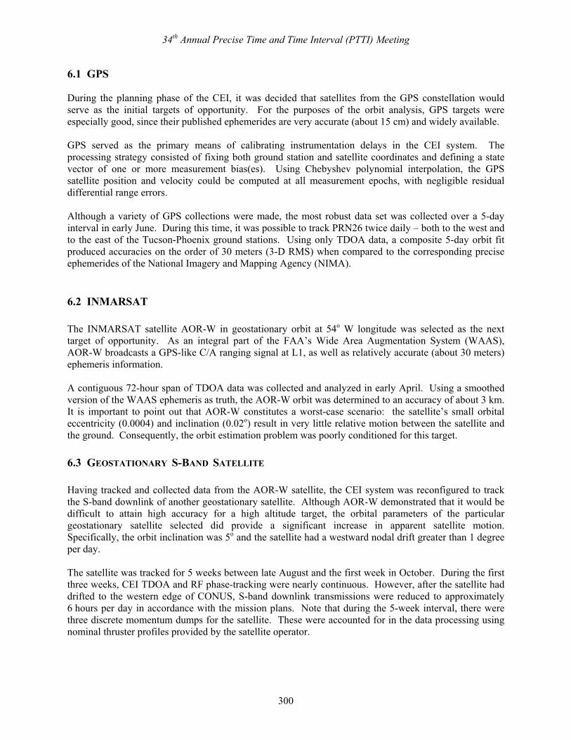
6.1 GPS During the planning phase of the CEI, it was decided that satellites from the GPS constellation would serve as the initial targets of opportunity. For the purposes of the orbit analysis, GPS targets were especially good, since their published ephemerides are very accurate (about 15 cm) and widely available. GPS served as the primary means of calibrating instrumentation delays in the CEI system. The processing strategy consisted of fixing both ground station and satellite coordinates and defining a state vector of one or more measurement bias(es). Using Chebyshev polynomial interpolation, the GPS satellite position and velocity could be computed at all measurement epochs, with negligible residual differential range errors. Although a variety of GPS collections were made, the most robust data set was collected over a 5-day interval in early June. During this time, it was possible to track PRN26 twice daily – both to the west and to the east of the Tucson-Phoenix ground stations. Using only TDOA data, a composite 5-day orbit fit produced accuracies on the order of 30 meters (3-D RMS) when compared to the corresponding precise ephemerides of the National Imagery and Mapping Agency (NIMA). 6.2 INMARSAT The INMARSAT satellite AOR-W in geostationary orbit at 54o W longitude was selected as the next target of opportunity. As an integral part of the FAA’s Wide Area Augmentation System (WAAS), AOR-W broadcasts a GPS-like C/A ranging signal at L1, as well as relatively accurate (about 30 meters) ephemeris information. A contiguous 72-hour span of TDOA data was collected and analyzed in early April. Using a smoothed version of the WAAS ephemeris as truth, the AOR-W orbit was determined to an accuracy of about 3 km. It is important to point out that AOR-W constitutes a worst-case scenario: the satellite’s small orbital eccentricity (0.0004) and inclination (0.02o) result in very little relative motion between the satellite and the ground. Consequently, the orbit estimation problem was poorly conditioned for this target. 6.3 GEOSTATIONARY S-BAND SATELLITE Having tracked and collected data from the AOR-W satellite, the CEI system was reconfigured to track the S-band downlink of another geostationary satellite. Although AOR-W demonstrated that it would be difficult to attain high accuracy for a high altitude target, the orbital parameters of the particular geostationary satellite selected did provide a significant increase in apparent satellite motion. Specifically, the orbit inclination was 5o and the satellite had a westward nodal drift greater than 1 degree per day. The satellite was tracked for 5 weeks between late August and the first week in October. During the first three weeks, CEI TDOA and RF phase-tracking were nearly continuous. However, after the satellite had drifted to the western edge of CONUS, S-band downlink transmissions were reduced to approximately 6 hours per day in accordance with the mission plans. Note that during the 5-week interval, there were three discrete momentum dumps for the satellite. These were accounted for in the data processing using nominal thruster profiles provided by the satellite operator.


301

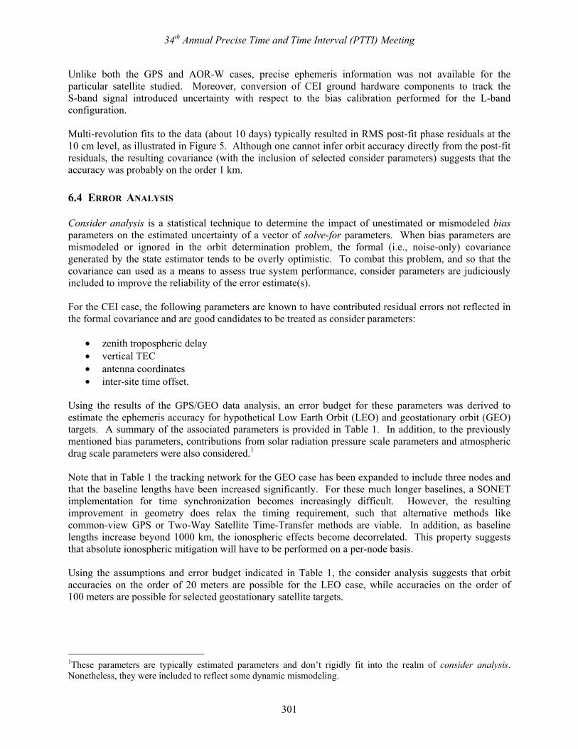
Unlike both the GPS and AOR-W cases, precise ephemeris information was not available for the particular satellite studied. Moreover, conversion of CEI ground hardware components to track the S-band signal introduced uncertainty with respect to the bias calibration performed for the L-band configuration. Multi-revolution fits to the data (about 10 days) typically resulted in RMS post-fit phase residuals at the 10 cm level, as illustrated in Figure 5. Although one cannot infer orbit accuracy directly from the post-fit residuals, the resulting covariance (with the inclusion of selected consider parameters) suggests that the accuracy was probably on the order 1 km. 6.4 ERROR ANALYSIS Consider analysis is a statistical technique to determine the impact of unestimated or mismodeled bias parameters on the estimated uncertainty of a vector of solve-for parameters. When bias parameters are mismodeled or ignored in the orbit determination problem, the formal (i.e., noise-only) covariance generated by the state estimator tends to be overly optimistic. To combat this problem, and so that the covariance can used as a means to assess true system performance, consider parameters are judiciously included to improve the reliability of the error estimate(s). For the CEI case, the following parameters are known to have contributed residual errors not reflected in the formal covariance and are good candidates to be treated as consider parameters:

• zenith tropospheric delay • vertical TEC • antenna coordinates • inter-site time offset.

Using the results of the GPS/GEO data analysis, an error budget for these parameters was derived to estimate the ephemeris accuracy for hypothetical Low Earth Orbit (LEO) and geostationary orbit (GEO) targets. A summary of the associated parameters is provided in Table 1. In addition, to the previously mentioned bias parameters, contributions from solar radiation pressure scale parameters and atmospheric drag scale parameters were also considered.1 Note that in Table 1 the tracking network for the GEO case has been expanded to include three nodes and that the baseline lengths have been increased significantly. For these much longer baselines, a SONET implementation for time synchronization becomes increasingly difficult. However, the resulting improvement in geometry does relax the timing requirement, such that alternative methods like common-view GPS or Two-Way Satellite Time-Transfer methods are viable. In addition, as baseline lengths increase beyond 1000 km, the ionospheric effects become decorrelated. This property suggests that absolute ionospheric mitigation will have to be performed on a per-node basis. Using the assumptions and error budget indicated in Table 1, the consider analysis suggests that orbit accuracies on the order of 20 meters are possible for the LEO case, while accuracies on the order of 100 meters are possible for selected geostationary satellite targets.

1These parameters are typically estimated parameters and don’t rigidly fit into the realm of consider analysis. Nonetheless, they were included to reflect some dynamic mismodeling.


302

Table 1. Consider Analysis Error Budget.

Orbit Regime LEO GEO Orbital Elements

a = 7204 km e = 0.001 i = 98.7o

a = 42164 km e = 0.0002 i = 0.001

Data Collection Tracking Nodes 2 3 Baseline Length(s) 180 km 1000 – 2000 km Tracking Rate Continuously @ 0.1 Hz1 5 minutes/hr @ 0.1 Hz Fit Interval 48 hrs 96 hrs

Consider Bias Parameters Time Synchronization 5 ns 10 ns ∆ Zenith Troposphere 10 cm 10 cm ∆ Vertical Ionosphere 80 cm 160 cm Station Coordinates 10 cm / axis 10 cm / axis

Consider Dynamic Scale Parameters Solar Radiation Pressure 5% of nominal 5% of nominal Atmospheric Drag 10% of nominal N/A

1 The satellite is tracked continuously when it is in view.

7. CONCLUSIONS A Connected Element Interferometer was successfully developed and deployed to collect both TDOA and differential RF phase data from a combination of mid- to high-altitude satellites for the purpose of satellite orbit determination. Using satellite targets of opportunity, including a GPS satellite and the INMARSAT geostationary satellite AOR-W, orbit accuracies on the order of 30 meters and 3 km, respectively, were attained based on comparisons to their corresponding published ephemerides. A more extensive data collection and processing effort was performed by sampling another geostationary satellite that has an S-band downlink. While it was not possible to assess the absolute accuracy of the ephemeris solution, the post-fit phase residuals were at the 10 cm level, demonstrating a high level of consistency between the coherent phase observations, the measurement model, and a high-fidelity dynamic model. The analysis of the data collected suggests that unmitigated atmospheric errors and residual instrumentation delays are the dominant errors sources for a tracking scenario consisting of a modest baseline (about 180 km). As a result of weak viewing geometry, system biases cannot be as part of the orbit determination process, emphasizing the importance of rigorous a priori system calibration. The anticipated performance of future CEI systems was also investigated via consider covariance analysis. Using an error budget derived from the pool of the collected data, ephemeris accuracy for hypothetical LEO and GEO targets was assessed. The covariance analysis suggests that the current Tucson/Phoenix configuration can provide LEO orbit accuracies on the order of 15 m to 20 m. By adding a third node and extending the nominal baseline lengths to 1000 km to 2000 km, orbit accuracies on the order 100 m should be possible for selected GEO targets. This augmented tracking network would likely


303

require an alternative timing mechanism such as common-view GPS or Two-Way Satellite Time Transfer. REFERENCES [1] G. Bierman, 1977, Factorization Methods for Discrete Sequential Estimation (Academic Press,

New York). [2] D. D. McCarthy (ed.), “IERS Conventions (1996),” IERS Technical Note 21 (International Earth

Rotation Service, Observatoire de Paris, July 1996). [3] P. Collins, R. Langley, and J. LaMance, 1996, “Limiting Factors in Tropospheric Propagation

Delay Error Modelling for GPS Airborne Navigation,” in Proceedings of the Institute of Navigation (ION) 52nd Annual Meeting, 21 June 1996, Cambridge, Massachusetts, USA (Institute of Navigation, Alexandria, Virginia), pp. 519-528.

Figure 1. Map of interferometer geography.


304

Figure 2. Diagram of CEI equipment at each site.


305

Figure 3. L-Band RF and calibration subsystem.


306

Figure 4. Typical time-based communications implementation.

Figure 5. Post-fit geostationary satellite phase residuals (10-day arc).

BLDG 1 BLDG 2

TSC SonetMaster

ATMSWITCH

ATMSWITCH

TSCSONET Slave

Master

Clock

OC-3 155.52 Mbs1300 nm SMF

SYNCHRONIZATION ERROR DEFINED ASTHE DIFFERENCEBETW EEN MASTER CLOCK AND SONET SLAVE SIGNALS

Slave

Clock

-5.0

-4.0

-3.0

-2.0

-1.0

0.0

1.0

2.0

3.0

4.0

5.0

0 24 48 72 96 120 144 168 192 216 240 264 288Hours Past 2002-Sep-01 00:00:00 UTC

R e s i d u a l s − m −


307

QUESTIONS AND ANSWERS TOM CLARK (Syntonics): Back in my days at Goddard, we did some very similar experiments using very long baseline interferometry systems. Bob Preston, now at JPL, and Marshall Eubanks, formerly at the USNO, both did significant studies tracking geostationary satellites at X-band using VLBI systems. And my group did some GPS tracking using VLBI systems. One comment I would make in terms of your error uncertainties, the 10-centimeter station errors seem to be, to me, rather gross. I would have thought that you would have had enough sensitivity – I calculated you had two-tenths of an arc second fringes, and you should have had a fair number of natural radio sources smaller than about a tenth of an arc second that you could have used for calibration in order to be able to solve both the atmospheric problems and the station location problems. So I would suggest that perhaps tying your measurements into the celestial reference frame would make a lot of sense here. DAN MORRISON: I think that you made some good points, Tom. The antenna locations were done by using commercial differential GPS surveying. And so, I think we were in a few- centimeter range on that, that really is not unrealistic. And I think in a system that was actually set up to be other than an experimental test bed, we would do a much higher precision job of that. KEN JOHNSTON (U.S. Naval Observatory): The thing that you have to remember, Tom, is that the signal you are looking at is like 10-26 watts per meter per hertz, so he is looking at a much stronger signal. So I don’t know if you have the capability to actually observe celestial radio sources. MORRISON: Well, first of all, the antennas that we were using, the most sensitive one was a 15-foot dish, 5-meter dish, and with a modest sensitivity LNA. So I think we would have been in trouble as far as that goes. In the case of the L-band stuff, we had a 5-meter dish combined with basically a choke-ring omni antenna. In the case of the S-band, we had two 1-meter dishes. So it was something that we thought about, and decided that it wasn’t going to buy us enough to go to the trouble to do it with this test.

ephemeris determination using a connected … · 34th annual precise time and time interval (ptti)...

Documents