eommhhhhmmhhhu mhhhhommmmu smhhmmhhmu …solid modeling is the subject of representing solid objects...
TRANSCRIPT
-A132 472 THE OCTREE ENCODING METHOD FOR EFFICIENT SOLID MODELING 1,/2
POECN LA 0JMEHE 'I(U) RENSSELAER POLYTECHNIC INST TROY NY IMAGE
UNCLASSIFIED N00014-2K 0301 F/ 9/2 N
EommhhhhmmhhhumhhhhommmmusmhhmmhhmuEommhhmmhhhhum

11-6
.4...
.;'
.4
1.8
HI"111II uI
MICROCOPY RESOLUTION TEST CHARTNATIONAL BUREAU OF STANDARDS -963-A
.11
IPL-TR-032
The Octree Encoding Method forEfficient Solid Modelipg
- Donald J. R. Meagher
August 1982
SEP 1 :983
bqU,
Appwl; •W Im P uW sg
Dbuzluaon Unft-.w
m. m.-o.r
Image Processing LaboratoryRensselaer Polytechnic Institute
STroY New York 12 18 183 09 13 038
,- ,a,,, ..,, ,.,.._ .,. .,.,. .

i2.
I PL-TR-032
The Octree Encoding Method for
Efficient Solid Modeling
Donald J. R. Meagher
August 1982
|DI
'-" L vslmbution Unutedltl _
Image Procesing LaboratoryEectrical and Systems Engineering DepartmentRensselaer Polytechnic Institute, Troy, New York 12181
!_ ,1

ABSTRACT
Solid modeling is the subject of representing solid
objects in a computer - to permit their analysis,
manipulation and display. This thesis describes the
•- development of a new solid modeling method called octree
-.. d9_ing, in which arbitrary objects are represented to a
/.specified resolution in 8-ary hierarchical trees or
: A-octrees. The number of nodes in an object's octree is
used as a measure of object complexity. This number is
shown to be on the order of the product of object surface
; area and the inverse of the square of the resolution.
A dual data-base approach is proposed. A
general-purpose solid-modeling system based on octree
encoding would interactively perform geometric, analytical
S'-and display operations in conjunction with specialized
%*::: .:: application data bases. k ---------------....
Efficient algorithms are presented for the
determination of mass properties (volume, surface area,
center of mass and moment of inertia, etc.) for the
formation of new objects via the use of set operations
(union, intersection, difference and negation), for linear
transformations (including translation, scaling and
L. rotation), for interference detection, for swept-volume
definition, and for display from any point in space (with
%ii• I "
* . . . . . . . . . . . .
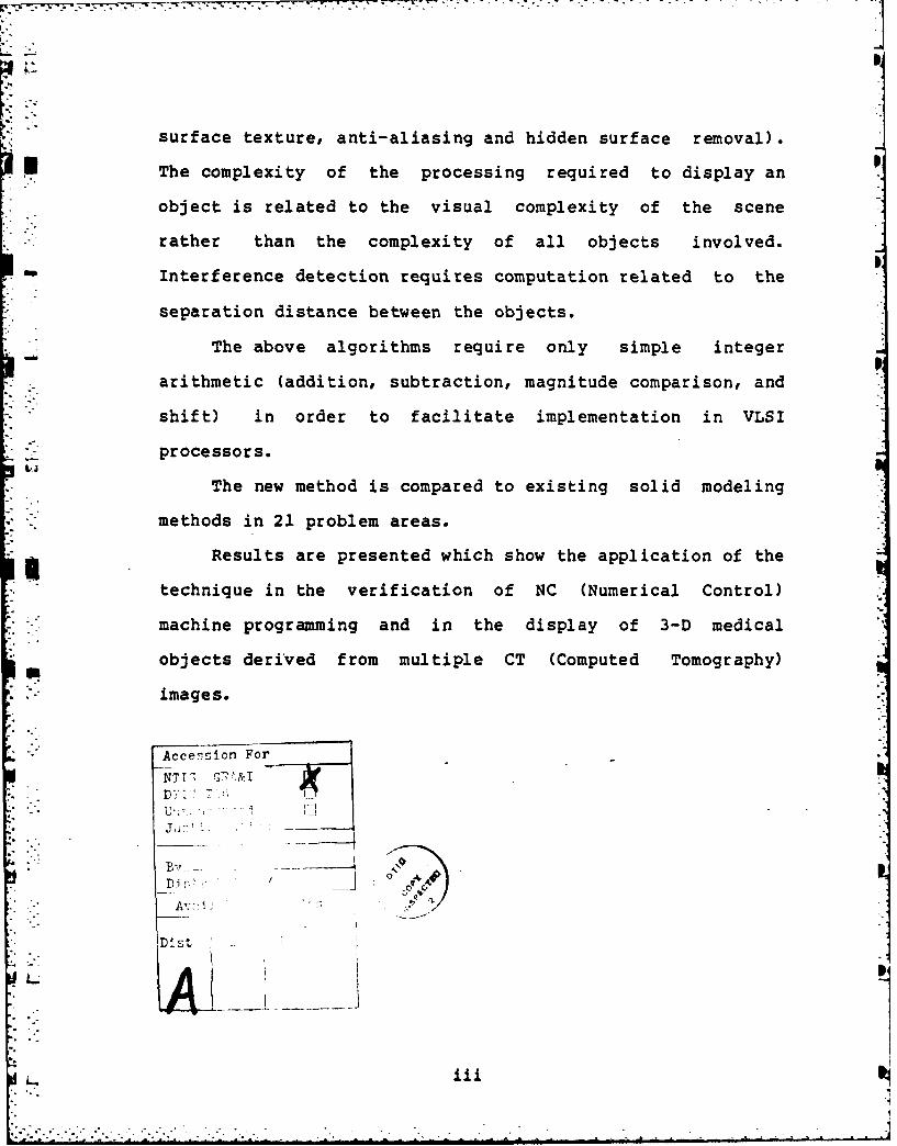
surface texture, anti-aliasing and hidden surface removal).
* i The complexity of the processing required to display an
object is related to the visual complexity of the scene
rather than the complexity of all objects involved. pInterference detection requires computation related to the
separation distance between the objects.
_ The above algorithms require only simple integer
arithmetic (addition, subtraction, magnitude comparison, and
shift) in order to facilitate implementation in VLSI
processors.
The new method is compared to existing solid modeling
methods in 21 problem areas.
a !Results are presented which show the application of the
technique in the verification of NC (Numerical Control)
machine programming and in the display of 3-D medical
objects derived from multiple CT (Computed Tomography)
images.
Accension For
NTT' G7 &T
Di,
, Dist
ii
!..

, ,..'. -. , - .-. ,, - - -' . ;-.. ..... ;,.., . 1, -. . --- 'I- . .- ,. .. ,, -.. ,. . - ,7
Table of Contents
, LIST OF FIRES.................. ...... *...*i.-- LIST OF TIGUES ........
!i~ ~ ~ LS OFi FIU ... o......................:)i CKNOWLEDGMENTo.o.... . . ...... .... ........... .. ...... ix
1. INTRODUCTION AND HISTORICAL REVIEW.......................11.1 Existing Solid Modeling Schemes. ................. 31.2 Historical Review...............................10
2 .H1.3 Approach... ....... .. .................. .. ... 14
2o THE OCTREE METHODo ... 19 ..~~~~~~.1 Definitions ................... . . . . . . . ..1
2.2 Object Representation......... .. ... o.o. 222 A Node Requirements...... ... .......... . o.o..... . 292.4 Complexity Metric 342.5 Storage Requirementso...... ................... 362.6 Expected Performance.... ....... ......... ... 38
n 3. OCTREE GENERATION....... ......................3.1 Algorithm Considerations..48 ..... . .. .o..o.48
3.2 Octree Generators......... ... .................. .503.3 Orthogonal Blocks ...... ......................... 553.4 Convex Objects.......o.... .55.... .... o.... .
4. ANALYSIS AND MANIPULATION.......o. ............. ... . 63
4.1 Object Properties...... . . . . .....o. . .... 634.1.1 Volume....................................634.1.2 Surface Area.o.... o. . ...... o. ... o . . . . ... .644.1 .3 Center of Mass. ............... ......... 644-,l.4 Moment of Inertia.........................65
a. 4.1.5 Segmentation of Disjoint Parts ............ 664.1.6 Interior Voids ............. ...... **.... .66" 4.1.7 Correlation ................ 66
4.2 Set Operations ......................... ......... 67
4.4 Geometric Operations ............................ 72• 4.4.1 Translationo ... ..... ..... ... ......... 72
4.4.2 Scaling .................................. 77:.4.4.3 Rotation.. . . . . . . . . . . . . . . . 794.4.4 Concatenated Geometric Operations ......... 84
iv
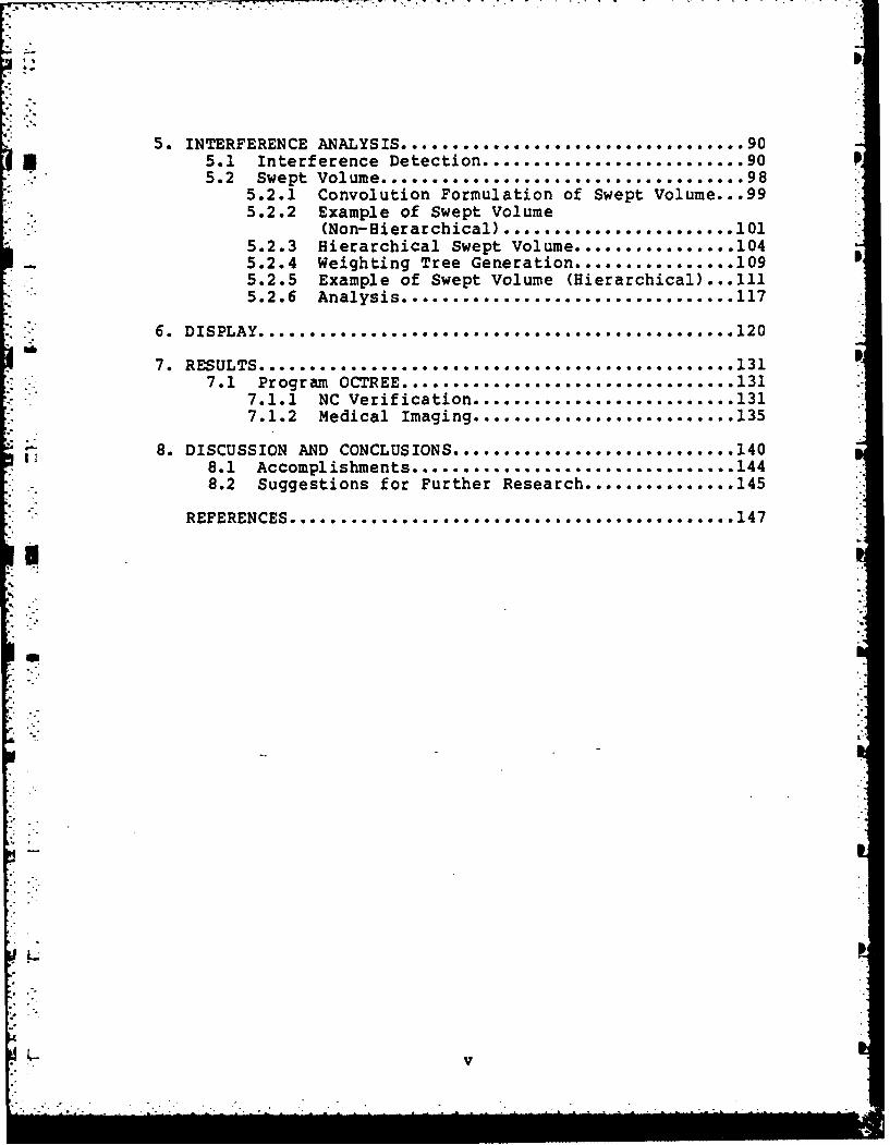
5.* INTERFERENCE ANALYSIS. . . ... .. .. .. . ... .. .. .. .. . .. *. . 90*5.1 Interference Detection .......................... 90
5.2.1 Convolution Formulation of Swept Volume ... 995.2.2 Example of Swept Volume
*(Non-Hierarchical) ...... ................. 1015.2.3 Hierarchical Swept Volume ................ 104
-5.2.4 Weighting Tree Generation ................ 1095.2.5 Example of Swept Volume (Hierarchical)...1115.2.6 Analysis .... ...... ............... 17
7.1 Program OCTREE. ... ... .. .... ...... ... ....... .... .1317.1.1 NC Verification ........ . .. .. .. .. . ... .. ... .1317.1.2 Medical Imaging ....... .. .. .. .. .. .. .. .. ... .135
8. DISCUSSION AND CONCLUSIONS.. ... ... .. . . .1408.1 Accomplishments ..... . .. . . .................... 48.2 Suggestions for Further Research ............... 145
REFERENCES ..... ............. . 4
,.1

LIST OF TABLES
Table 2.1 Tabulation of Resolution and Expected PgNode Count ** ****.......................... 42
t
vi
LIST OF FIGURES
Page
Figure 2.1 Child and Vertex Labeling .................. 25
Figure 2.2 Sample Octree .............................. 26
Figure 2.3 Minimum-Surface Representable ObjectWhich Touches 9Obels ...................... 31
Figure 2.4 Area of Object ............................. 32
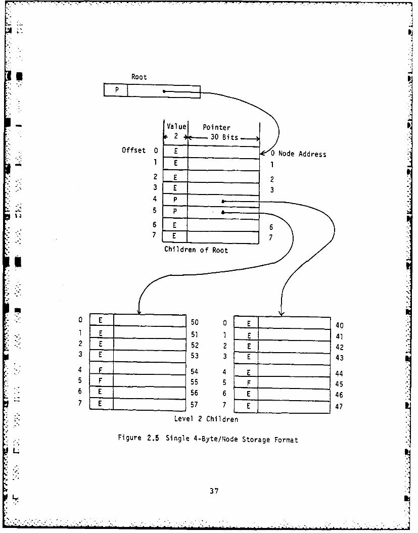
Figure 2.5 Single 4-Byte/Node Storage Format ........... 37
Figure 2.6 Edge of Object Cuts Obel and IntersectsObel Diagonal ............................... 40
Figure 3.1 Octree Generator ........................... 52
Figure 3.2 Calculation of Child Vertex CoordinatesFrom Parent Values .......................... 54
Figure 3.3 Octree Generation for 3-D OrthogonalmBlock ...................................... 56i-
Figure 3.4 Generation Terms for Child Obel fromParent Values ............................... 60
Figure 4.1 Example of Octree Set Operations ........... 68
Figure 4.2 Overlay Structure .......................... 74
Figure 4.3 Three-Dimensional Overlay .................. 75
Figure 4.4 Example of Octree Translation .............. 76
Figure 4.5 Example of Octree Scaling .................. 78
Figure 4.6 Example of Octree Rotation by 90 Degrees ... 80
Figure 4.7 Rotation Overlay........................... 81
Figure 4.8 Example of Octree Rotation by ArbitraryAngle (27.8 Degrees) ....................... 83
Figure 4.9 Target Obel for Concatenated GeometricTransformation ............................. 85
Figure 4.10 Transformed Coordinate Value ............... 87
vii
. ...
Figure 4.11 Target Obel for 3-D Concatenated GeometricTransformation . ... .. .... ... ... ...... .. ..... 88p
Figure 5.1 Interference Detection Universe Pointers ... 95
Figure 5.2 Swept Area . .... *...... .... .. . .... .... .. .... . 102KFigure 5.3 Weighting Pattern .......................... 103
Figure 5.4 Distribution of Children Input Node/Weighting*.Node Pairs for 1-D Sweep Left .............. 108
*Figure 5.5 Weighting Tree Generation .................. 112
Figure 5.6 Object tobe Swept........................ 114
Figure 5.7 Example of l-D Sweep Algorithm ............. 115
Figure 6.1 Hidden Surface Traversal Sequence .......... 121
*Figure 6.2 Octree Object Nodes (Cubes) Are WrittenInto Display Screen Quadtree ............... 123
Figure 6.3 Projection of Node (Cube) on Display Screenand Overlay Structure ............. *006.0-.. 124
* -*Figure 6.4 Octree Representation of Turbine Blade ... 128
Figure 6.5 Illumination Plane (Quadtree) ProjectsIllumination on object Node .... ............ 130
*Figure 7.1 Simulated Milling Operation ................ 134
Figure 7.2 Display of Section of Human Skull ....... 136
Figure 7.3.. Display of Sinus Passages ............... 138
viii

ACKNOWLEDGEMENTU
The author wishes to express his appreciation to
Professor Herbert Freeman of the Electrical, Computer and
Systems Engineering Department and Director of the Image
Processing Laboratory (IPL) at Rensselaer Polytechnic
* . Institute for the guidance, support and encouragement
received under his supervision.
The author would also like to thank Professor W.
Randolph Franklin, the other committee members and Dr.
Michael Potmesil for their assistance and suggestions.
* This research was funded in part by the National
Science Foundation's Automation, Bioengineering and Sensing
Program under grant ENG-79-04821 and in part by the Office
of Naval Research under Contract N00014-82-K-0301,
NR049-515. Development of the NC verification system was
funded by the Center for Manufacturing Productivity and
Technology-.Transfer (CMP/TT) at RPI. Development of the
swept volume and display algorithms was sponsored by Phoenix
Data Systems, Albany, New York.
'4
* .
aix
-p,
* . - .
CHAPTER 1
*! p
INTRODUCTION AND HISTORICAL REVIEW
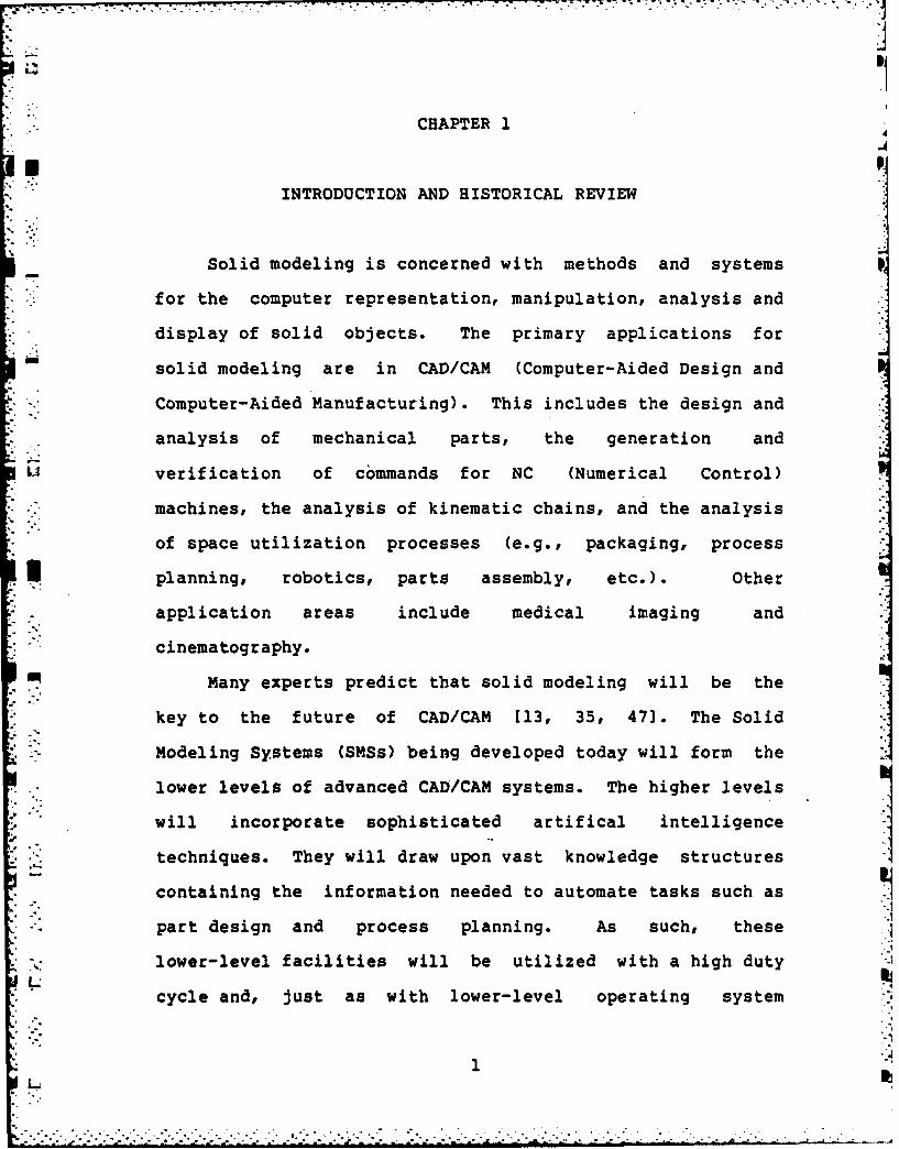
Solid modeling is concerned with methods and systems
for the computer representation, manipulation, analysis and
- display of solid objects. The primary applications for
- solid modeling are in CAD/CAM (Computer-Aided Design and
SComputer-Aided Manufacturing). This includes the design and
* analysis of mechanical parts, the generation and
u verification of commands for NC (Numerical Control)
* machines, the analysis of kinematic chains, and the analysis
of space utilization processes (e.g., packaging, process
S planning, robotics, parts assembly, etc.). Other
application areas include medical imaging and
cinematography.
Many experts predict that solid modeling will be the
key to the future of CAD/CAM [13, 35, 471. The Solid
Modeling Systems (SMSs) being developed today will form the
lower levels of advanced CAD/CAM systems. The higher levels
- will incorporate sophisticated artifical intelligence
techniques. They will draw upon vast knowledge structures
containing the information needed to automate tasks such as
part design and process planning. As such, these
lower-level facilities will be utilized with a high dutyL
cycle and, just as with lower-level operating system
°.1

procedures, must be made fast and efficient. They must be
extremely reliable and completely automatic. Human
intervention to resolve ambiguities obviously could not be
tolerated.
Although there are currently more than 20 major SMSs,
they are all limited to a greater or lesser degree because
of deficiencies in object representation and processing-
algorithms (54]. Two major shortcomings will be mentioned.
First, representation capabilities are not sufficiently
robust easily to handle the object complexities required in
a realistic environment. Second, the manipulation and
display algorithms for such functions as interference
detection (two or more objects occupying the same space) and
hidden-surface removal (necessary for realistic display)
require extremely large numbers of calculations in practical
situations. They usually exhibit polynomial growth (often
quadratic) in the number and complexity of the objects.
The goal of this research has been to devise a new
object representation scheme and associated linear growth
algorithms in which objects of abitrary complexity tan be
encoded, manipulated, analyzed and displayed interactively
_ein low-cost hardware. A solid modeling method called octree-
encoding was developed. The technique is based on a
hierarchical 8-ary tree or moctree."
This researchl was conducted over a period of almost
five years. This thesis is the seventh in a series of
2
publications documenting the work [38-431. The major
results are presented here, with the earlier reports
referenced for supporting information.
1.1 Existing Solid Modeling Schemes
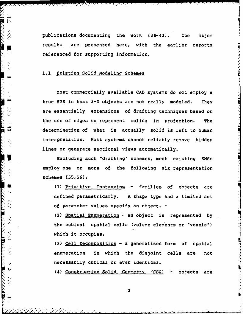
Most commercially available CAD systems do not employ a
true SMS in that 3-D objects are not really modeled. They
* [are essentially extensions of drafting techniques based on
the use of edges to represent solids in projection. The
determination of what is actually solid is left to human
. -interpretation. Most systems cannot reliably remove hidden
lines or generate sectional views automatically.
. Excluding such "drafting" schemes, most existing SMSs
employ one or more of the following six representation
*i schemes [55,561:
P (1) Primitive Instancing - families of objects are
defined parametrically. A shape type and a limited set
of parameter values specify an object. -
(2) Spatial Enumeration an object is represented by
the cubical spatial cells (volume elements or "voxels")
which it occupies.
(3) Cell Decomposition - a generalized form of spatial
enumeration in which the disjoint cells are not
necessarily cubical or even identical.
(4) Constructive Solid Geometry (CSG) - objects are
3

represented as collections of primitive solids (cuboids,-9
cylinders, etc.). A tree structure is typically used
with leaf nodes representing primitives and branch nodes
specifying set operations.
(5) Sweep Representation - a solid is defined as the
volume swept by a 2-D or 3-D shape as it is translated
along a curve.
(6) Boundary Representation (B-Rep) - objects are
represented by their enclosing surfaces (planes, quadric
surfaces, patches, etc.).
Specific advantages and disadvantages of each have been
tabulated [57] along with a classification of 21 existing
* systems. For a primary representation scheme, most use CSG
(TIPS, PADL, SynthaVision, etc.) or B-Rep (Build, CADD,
Design, Solidesign, Romulus, etc.) or a combination of the
two (EUKLID, GMSolid). Often other formats are used for
secondary functions. Some allow alternate representations,
such as swept volume, for input. Some have special features.
For example, TIPS sorts the primitives into a spatial
enumeration array to facilitate interference analysis. In a
separate study, Baer, Eastman and Henrion (3] have analyzed
and compared 11 popular systems. Much information has
recently become available on specific systems (7-9, 10, 11,
28, 36, 49, 61, 80, 82].
New methods are needed to solve or at least reduce the
4
7777--7 71*:1.
following problems which have been found to plague (to a
*greater or lesser extent) systems based on the above six
schemes (see [27, 56]).
(1) Limited domain -The currently used schemes are
characterized by a restricted domain of representable objects
because they are constructed from a limited number of
mathematically well-dfndsraeo oi primitives.
Some systems allow quadric surfaces and higher-order patches.
This can limit performance, however, because the more general
and more powerful primitives usually require substantial
* additional computations for object manipulation and display.
Adding a new primitive to a system or generalizing the use of
an existing one may necessitate extensive development of
5 mathematical tools and significant software modification.
* - -Another consideration is the potentially large labor cost
involved in what is essentially the art of fitting primitives
to a desired object.
(2) Validity - In many schemes, not all objects which
can be created are true or valid 3-D objects (also called
well-formed" objects). The 'intersection of two objects, for
example, may create *nonsense objects" such as dangling edges
or faces bounding no volume. Some systems depend upon human
intervention to eliminate such artifacts. Others contain ad
hoc algorithms to detect and eliminate invalid elements after
each operation. A few make such checking an integral part of
the manipulation algorithms. In any event, it adds overhead
5
and reduces the efficiency of a scheme. Ideally, any object
which can be legally generated should correspond to a valid
object.
(3) Completeness - A complete representation contains
all the information required to determine the interior and
exterior of an object. There should be no ambiguity. All of
the aforementioned schemes are (or can be made) complete
representations and, in fact, completeness is required for a
true SMS. It may be costly in overhead processing, however.
(4) Uniqueness - If a SMS is unique, there is only one
possible symbol structure for a given object, regardless of
position or orientation. This simplifies object matching and
identification, which may be important in some applications.
However, most existing schemes are not unique.
There are two common causes of nonuniqueness:
permutational nonuniqueness in which substructures in the
symbol structures can be permuted, and positional
nonuniqueness in which different representations correspond
to the same object but at different- positions or
orientations.
(5) Conciseness - There are two parts to conciseness.
Basically, it refers to the amount of data (bytes, for
example) required to represent an object. If an object can
be represented in a scheme with fewer words of storage, then
it is more concise. A deeper meaning takes into account the -
size of the domain of representable objects. A valid
6
comparison of conciseness can only be made between two
systems when both are configured to represent the same set of
"- possible objects to the same precision, usually a very
" difficult, if not impossible, task.
(6) Closure - A SMS has the property of closure if the
results of any object operation can be used as input for
further operations.
(7) Finiteness - It should not be possible to create
-- objects with infinite volumes.
(8) Null object - It should be easy to determine whether
an object is null (contains no volume).
- -. (9) TransDortability - Object representations should be
able to be transported to alternate computer facilities
5without inadvertant modifications resulting from a change in
word size, floating-point precision, etc. In addition,
identical operations on all machines should generate
*I identical results.
(10) Extensibilitv- The initial implementation of a
solid modeling system should be easily extended for modeling
larger, smaller or more complex objects, a larger number of
objects, sculptured surfaces, objects to a greater precision,
7 etc.
(11) -utonom The scheme should not require human
. intervention under any circumstances.
(12) Reliability - All possible objects (or at least all
SL objects which could be required) should be able to be
7
.. ..-. * . . . . . . - .. - . -. .

processed by all operators without error. In some systems,
for example, self-intersection is a fatal condition.
(13) Efficiency - The computational complexity and
resource requirements (memory, for example) of algorithms
should not grow faster than linearly in the number and
complexity of objects. In addition, it would be very
desirable if the instantenous computational load were related
to the actual complexity (in some sense) of the specific user
requested task rather than the overall number and complexity
of objects involved.
(14) Implementabilit7 - An SMS should be easily
implemented for a large range of practical tasks on existing
computers or in hardware utilizing current or near-term
technology. A scheme will be more easily implementable if
the number of calculations are small relative to the number
of objects and object complexity. Also, algorithms requiring
simple mathematical operations and those allowing extensive
paralleling or pipelining of operations will be easier to
implement in the VLSI (Very-Large-Scale Integration) environ-
ment of the future.
Many of the existing SMSs were designed when an
evaluation of the hardware requirements called for compact
data structures and algorithms that would fit into limited
memory (typically 64K bytes). Calculations were to be
handled by a single, serial processor, most often a -
general-purpose minicomputer. This stategy has resulted in
8
-. -- .:
schemes that may be very efficient in memory usage but often
require unrealistically large numbers of calculations,
usually in floating-point rather than integer arithmetic. A
more realistic appraisal of current hardware trends could
result in more powerful and easily implementable schemes.
(15) Multiple representations - For a broad-based
application, two or more representation schemes may need to
be maintained to handle all requirements. Experts in the
field seem to agree (reluctantly) that this will be
necessary, given the limitations of the six representation
schemes.
.. (16) Consistency- If multiple representation schemes
are maintained, they should be guaranteed to be consistent at
" all times. If two representations of a single object could
be contradictory, an application system would probably be
useless.
I (17) Conversion - If multiple representations are used,
a method to convert from one to another is required. The
transformation should be exact (rather than approximate) and
invertable. In general, however, this is not the case with
existing schemes.
(18) Ease of object creation and manipulation - In
. general, a system that allows a user more easily to generate
and manipulate any desired object will be more useful. A
short response time is desirable, for example.
(19) Finite-element modelinq capability - It is an
9i.mJ

advantage if a scheme can easily and automatically generate a
finite-element mesh in 3-D.
(20) Interference analysis - Many applications require
the detection of interference between two or more objects.
The generation of a hidden surface view can be thought of as
a visual interference problem. The development of linear
growth algorithms involving interference was a major
objective of the research described in this thesis.
(21) Tweakinq - It should be possible to make local
changes without involving the entire object.
1.2 Historical Review
The solid modeling method described here results from a
doctoral program undertaken by the author in September 1977.
In the spring of 1978 a literature survey of techniques for .
representing and analyzing shapes was carried out, with an
emphasis on 3-D techniques [38].
In the-.fall of 1978 the-general goals of the research
effort began to take form. A new solid modeling method would
be developed to alleviate many of the common problems
encountered with existing systems, especially when applied to
large-scale efforts in CAD/CAM. The primary consideration
was to develop a simple, powerful, efficient and fast scheme
that could be easily implemented in VLSI for future
"real-world" applications of great complexity.
10
.T'. '" ' ? . '. .. "- i . - T L • . . .L .... , .== " ' " . . - - -. = - " ° -

W W . - -
The coding of what later became the program OCTREE began
in October 1978. The outline of a new technique employing
hierarchical tree structures was defined and first
implemented in a 2-D scheme called "area encoding." By the
spring of 1979, algorithms had been developed and implemented
for the entry of 2-D chain codes, conversion to an area
encoded format, and generation of the intersection of two
objects.
At about the same time, April 1979, the first widely
distriouted paper describing a similar 2-D technique with
applications in a different area, image processing, was
published by Hunter and Steiglitz [29]. Based on Hunter's
PhD thesis (30], it made use of 2-D hierarchical tree
structures called "quadtrees" (also called "quad-trees" or
"quad trees").
Further investigation turned up a proposal by Tanimoto
* S [78] to use a "pyramid" image model as a measure of binary
image complexity. Additional quadtree publications have
appeared in.. the literature-since that time; Rosenfeld (58,
59] has pursued quadtree efforts in pattern recognition and
image processing. Samet has presented an overview of
quadtrees (with Rosenfeld) (72], and developed quadtree
0algorithms to compute the perimeter [65], convert from
boundary codes [68], to boundary codes (with Dyer and
Rosenfeld) (19], from raster format (69], to raster format
[70], from binary arrays (71], compute the medial axis
11
• ' i i . . . ._t.-i - .-" ... . .. ..- - - - - . .. .. _.' - .... , .. .: . . ...

transformation [63], compute a distance function [64], find
neighbors [671, and label connected components [66]. Shneier
has developed algorithms to calculate geometric properties of
quadtrees [74]. Ranade has employed quadtree techniques for
edge enhancement [511, and (with Shneier) for image smoothing
[50, 52]. Hunter and Steiglitz have presented an algorithm
to perform linear operations on quadtrees based on _
transforming edge segments (31]. Burt has developed the
"hierarchical discrete correlation" (HDC) for efficient image
processing [12].
The effort continued during the summer of 1979 with the
development of the "overlay" technique for efficiently
performing linear operations on objects and the basic hidden
surface display algorithms. Much of this was implemented and
verified during the fall of 1979.
In October 1979 a presentation of the technique was made
that included computer output examples of translation,
rotation (90-degree, 180-degree and arbitrary-angle), union,
intersection, difference, reflection about- an axis, 2-D
hidden-line elimination and 2-D perspective display. At
about this time the name "octree encoding" was given to the
technique (it had earlier been called "volume encoding").
In the spring of 1980, a report was written to present
the scheme. It was first submitted in July of 1980 and later
published as an IPL technical report [391. Additional
results were presented in a paper titled "Geometric Modeling
12
Using Octree Encoding.w It was submitted in December 1980
and released as an IPL technical report [40]. A slightly.'updated version was published in Computer Graphics and Image
Processing 144].
The Octree Encoding scheme was presented in the Computer
Graphics course at RPI during the Fall of 1980 and officially
proposed as a PhD thesis topic in March 1981.
The advanced display algorithm presented below was
developed during the spring and summer of 1981. It was first
described early in September 1981 and, later that month, a
paper describing the technique was presented at the IEEE
Computer Society's Tenth Workshop on Applied Imagery Pattern
Recognition (AIPR) in College Park, Maryland. The paper was
5 also released as an IPL technical report (41]. An updated
version was presented at the IEEE Computer Society's Pattern
Recognition and Image Processing (PRIP) conference in June
01 1982 [45].
The whierarchical convolution" technique and its
application..to swept volume-generation were-developed during
the Fall of 1981. The swept volume algorithm was first
presented in November 1981. The algorithm is described
below.
A major effort in late 1981 and early 1982 was devoted
to efficient object generation algorithms. These and other
results are documented in an IPL technical report [43].
" - LThe general idea of hierarchical geometric models as the
13
basis for future hidden-surface algorithms was proposed by
Clark [16]. Multidimensional binary trees and algorithms
have been studied by Bentley for use in data base
applications [4, 6]. Franklin has developed the "variable
grid" technique for hidden line and surface applications -
[21-23]. It is shown to be a linear growth algorithm at the
expense of pre-sorting. This has been extended into a
hierarchical structure in Octree Encoding and forms the basis
of the linear computational characteristics of the scheme.
Rubin and Whitted [621, Reddy and Rubin [53], Fuchs
[251, and others have presented various object space
pre-sorting techniques. The use of 8-ary hierarchical trees
to represent 3-D objects was apparently first suggested by
Hunter [30] in his PhD thesis (1978) as a possible extension
of quadtrees. It was later independently proposed by Jackins
and Tanimoto [33, 34], Moravec [46], Srihari [75, 76] for
medical imaging, Meagher [391 and perhaps others. Later
octree reports include [17, 18, 32, 861.
1.3 Approach
The ultimate goal of this effort has been the actual
construction of a full-function, real-time (about 1/30 second
response) solid modeling system to handle any number of
arbitrarily complex objects while operating on relatively -
low-cost hardware. Conventional solid modeling wisdom
14
"+ . . ,,/ + . ' . . . . . . . . .

assumed that these characteristics were mutually exclusive.
Levels of performance many orders of magnitude greater than
" - allowed by existing techniques are needed. Obviously a new
approach was required!
The remainder of this section is a summary of the four
or five years of evolving reasoning and philosophy embodied
- *in the octree encoding method. A more in-depth study is
presented in (431.
' .*The first step was to reject any preconceived ideas
about solid modeling. An entirely new method would be
designed and developed. A list of priorities was established
-..2 for guidance and direction. The highest priority throughout
the effort was high-speed operation. For the first few years
5 the actual usefulness of the method was open to question but
there was never doubt the functions could be performed at an
extremely. high throughput utilizing modest hardware.
, NThe second priority was robustness. This included both
the ability to represent arbitrary objects and a full
complement of analysis, manipulation and display functions.
The third thrust was a general drive for simplicity.
This required, for example, a single representation scheme
for all objects and very simple algorithms.
Given these general priorities, the first step was to
devise a solution to the object storage problem. Arbitrary
objects require arbitrary quantities of storage for
representation. It was decided to represent arbitrary
15
L
°-,.

objects to a variable but limited precision.
CSG schemes handle this dilemma by taking what can be
looked at as the opposite choice. Unlimited resolution (for
all practical purposes) is preserved but objects are
restricted to primitive analytic shapes or combinations-
thereof.
The next step was to address the computational
complexity issue. Most existing CAD systems have evolved
from attempts to automate 2-D drafting. Complexity has not
generally been a consideration because the typical drafting
task is linear in a small number of items. Interactive
operation is not difficult to achieve.
The progress of CAD into full 3-D applications has
changed the situation. Operations involving some form of
interference analysis have been found to require large, often -
prohibitively large, computational resources for interactive
operation. The root of the problem is a comparison task.
Naive algorithms perform an interference detection operation
by checking-. for intersection between each possibly relevant
pair of primitives. A combinatorial explosion results
because, in general, the number of pairs grows quadratically -
in the number of primitives.
The solution was to design a spatially pre-sorted
representation scheme that would never require additional
sorting or extensive searching. The octree scheme satisfies
this requirement.
16

9, S t,
The philosophical approach adopted for algorithm
development was based on the hierarchical ideas of Clark [16]ipU and the sharing of partial calculations that has been proved
so successful in the Fast-Fourier Transform (FFT). It is the
hierarchical structure into which the problem has been cast
*. that allows large numbers of low-level calculations to be
eliminated at an early stage when processing typical objects.
-mThe approach to actual implementation adopted for this
*effort was based on the current trends in VLSI technology.
It is clear that to maximize the performance-to-cost ratio,
7 full advantage should be taken of the tremendous improvementsI.
in hardware which have resulted and will no doubt continue to
result from VLSI.
Before proceeding, a popular misconception concerning
increased computing power should be dispelled. The tought
" "that increasingly powerful hardware at lower cost will allow
ON inefficient algorithms to become useful is, in general,
wrong. Other factors being equal, a performance increase
. will allow ..larger problems. to be handled,-further widening
the performance gap between an inefficient (quadratic growth,
* for example) algorithm and an efficient (linear) algorithm.
.*Thus, computational complexity issues become more, not less,
important as technology moves into the VLSI age. 0
The implementation approach was to develop algorithms
designed specifically for semi-custom or full-custom VLSI
L based operation. This decision impacted the entire design
17
*1,

1.71
philosophy. Traditional solid modeling systems tend to be
huge, ever growing, ever changing, software packages with
complex internal structures. The VLSI based system, in
contrast, must be based on a small number of very simple,
fixed, powerful and extremely reliable algorithms. They are
implemented in hardware and form the primitive lower level
functions in an applied system.
Based on the simplicity and ease of implementation
requirements, algorithms were allowed to employ only integer
numbers and only simple arithmetic (addition, subtraction,
magnitude comparison and shifts). Neither floating-point
operations, integer multiplications nor integer divisions
l were allowed.
.4
18-I
T?7
CHAPTER 2
THE OCTREE METHOD
2.1 Definitions
- A graph G(N,P) is a finite, nonempty collection N of
nodes and a set P of unordered pairs of distinct nodes called
edges. Two nodes connected by an edge are adiacent nodes.
K4 If an edge has an associated direction, it is a directed
*_-. The direction is from the tail node to the bg" node.
A graph containing only directed edges is a directed graph.
The number of edges having a particular node as their tail
node is the outdegree of that node. The number of edges
having a particular node as their head node is the i r
* ,of that node.
A 2_l is a sequence of edges connecting two nodes. For
a directed graph, the nodes visited must be -in tail-to-head
order. A graph containing no paths which originate and end
in the same node is called acyclic.
A tree is an acyclic directed graph in which all nodes
have indegree 1 except one node, the root, which has indegree
0. Any node with outdegree 0 is called a terminal node or
leaf. Nodes with outdegree greater than 0 are branch nodes.
L The level of a node is defined as the distance in edges from
19

the root. The root is at level 0.
The root is assumed to be at the top of the node
structure and all other nodes exist below the root. All
nodes reachable from a particular node are called the
descendants of that node. All nodes from which a particular -
node can be reached are the ancestors of that node.
Descendants one level below a node are the ciren of thatipnode. The ancestor adjacent to a node is the parent of that
node. Nodes having a common parent are siblings.
If a node does not actually exist in a tree but can be
inferred from an existing terminal node which would be one of
its ancestors, it is called an implied node. Loosely,
operations on a tree which use implied nodes are said to
process the implied tree rather than the actual tree.
Every branch node is a root of one or more subtrees.
The degree of a node is the number of subtrees that exist for
that node. If the outdegree of every branch node is <= m,
the tree is an m-ary tree. If the outdegree of every branch
node is m, the tree is a complete m-ary tree;
An m-ary tree is Ptionl if the children have m
distinct positions. The position is indicated by a value
from the child number set {0,l,2,...,m-l). Every node is
uniquely identified by a string over the child number set,
the node address. The root is represented by the empty
string. The node address of a child is the child number
prefixed by the address string of its parent.
20
" iA tree will be called a hierarchical tree if the
children of a node are associated with their parent in some
particular relationship.
* All objects exist within the universe. It is a finite
section of N-dimensional space defined by N orthogonal axes
and O<=x(i)<-d where x(i) is a displacement in dimension i,
(x(l), x(2),...,x(N)) is a point in the universe, d is the
length of an edQe of the universe and N is the order of the
" universe (number of dimensions). The symbol "N" will be
reserved for the order of the universe throughout this
thesis.
* .i Note that all edges of the universe have the same length
and form a square for N=2, a cube for N=3 and an
U N-dimensional hypercube for N>3. The origin of the universe
is the point of intersection of the axes. Negative
* displacements from the origin are not allowed. The space
* beyond the universe is the v No object can exist in the
void. Any part of an object moved into the void is
annihilated.- An augmented universe is one ifi which one or
. more adjacent (empty) universes are added to the P
universe. Augmented universes are used to facilitate
-".. algorithm initialization.
Before encoding, objects are called real objects. They
* may be real-world objects or a mathematical description of an
- ideal shape. An object encoded in the octree format is knownL
as the encoded object or simply the object.
21

mS
If a single encoded object is used many times to
generate new, transformed objects, the original object is the
model and the new objects are instances.
An object is always of the same order as the universe in
which it is defined and is composed of discrete units of
N-dimensional space. All objects in a third order universe
must occupy volume, for example. A 2-D object could not
exist here. The smallest object in such a universe would be
the smallest resolvable unit of space.
Other than this, there are almost no restrictions on
objects. They can be concave as well as convex, have
interior voids, and can be simply- or multiply-connected.
Each object is defined over the entire universe. It has
a property value defined at each point in the universe. For
a typical small object (relative to the universe) most of the
space in the universe has the property of being empty.
2.2 Object Representation
During the design and development of the object
representation scheme, the primary considerations were the
need for a spatially sorted format to eliminate the quadratic
growth of algorithms and the desirability of a hierarchical
structure to reduce the volume of data that would need
processing for a typical solid modeling operation. A third
consideration was the simplicity of algorithms that could
22
_7- - -I i , .-°
I" result if a regular spatial structure was used.
To facilitate spatial sorting, orthogonal planes were
used to segment object space. The need for a hierarchical
structure was satisfied by employing trees in which the
children represented the same space as the parent but to a
higher precision. To fulfill the requirement for a regular
structure, nodes at a given level represent disjoint segments
of space, are identical size, shape and orientation, and
completely fill the universe when all possible nodes are
taken together. The result was a recursive subdivision of
space with objects represented by cubes of exponentially
related size.
An octree object is represented by an 8-ary hierarchical
* tree or octree. Each node represents a cubical section of
the universe and contains a property value associated with
*-- the cube. In its simplest form, the property has one of 3
values. If the space is completely occupied by the object,
" the node has the value F (for "full"). If completely
disjoint, the value is E (for "empty"). If-neither occupied
nor disjoint (at least part of the object's surface is within
the cube) it has the value P (for "partially occupied"). The
property value is often loosely used as a node qualifier.
For example, a "P node" is a node with a property value of P.
The 8 octants of the cube represented by a node are, in
turn, represented by the node's 8 children. An octree is
L hierarchical in that the children, taken together, represent
23
exactaly the same space as the parent.
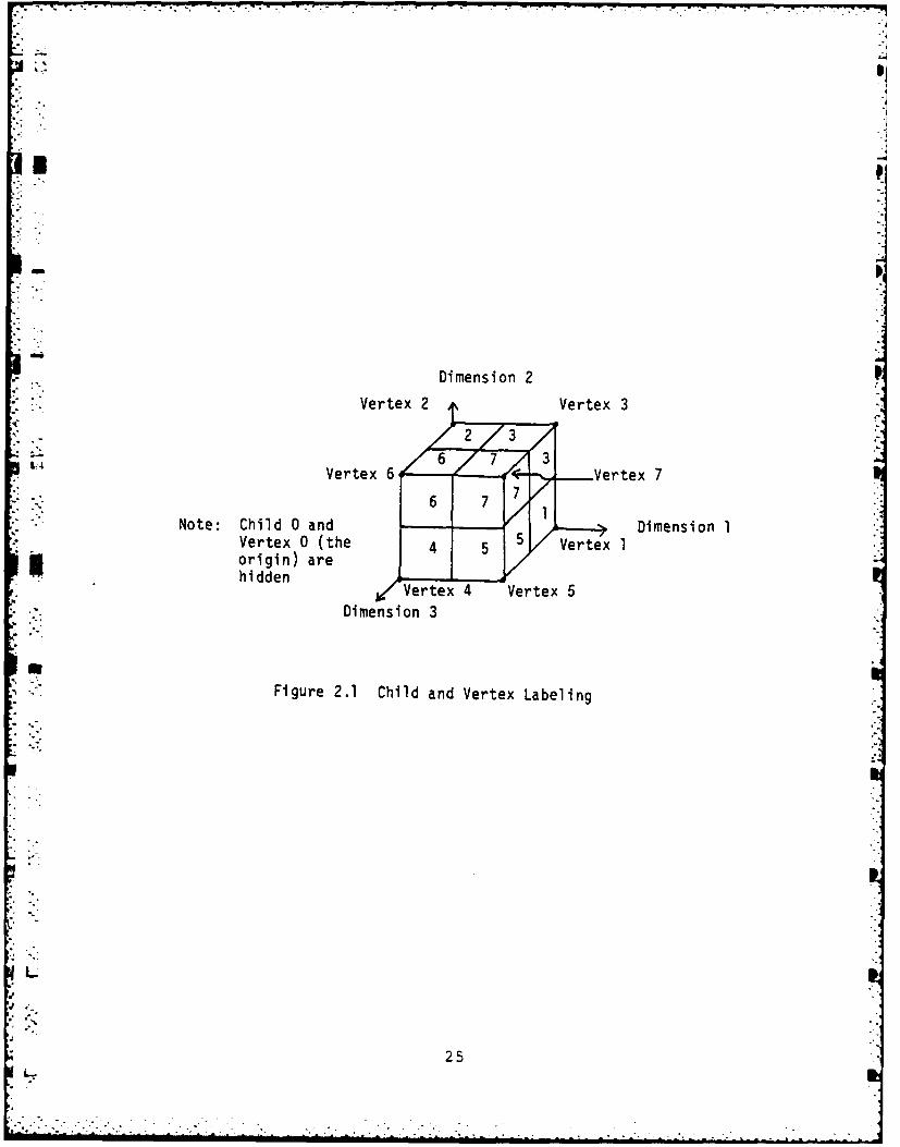
The correspondence between octant and child number is
defined in 2.1 along with the vertex labeling convention. A
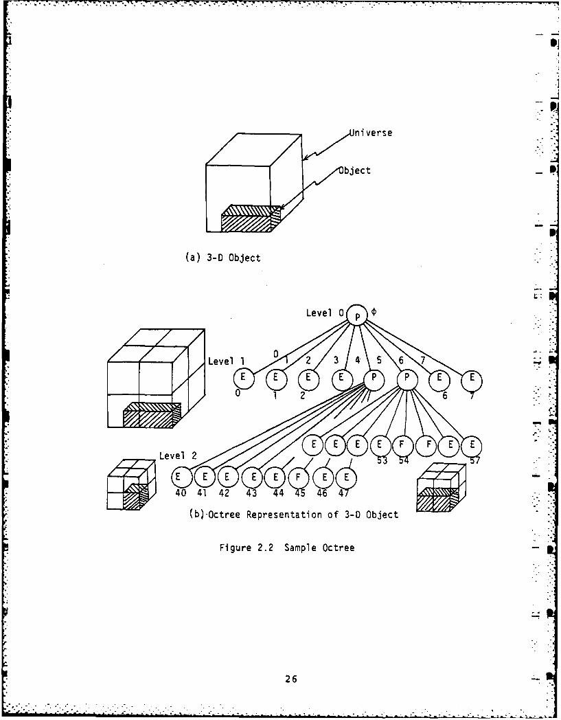
sample object and the universe are shown in 2.2(a). In
2.2(b) the corresponding octree is presented. The root node
at level 0 represents the entire universe and is given the
value P. At level 1, of the 8 octants of the universe, 6 are
empty and given E values. Two are partially occupied and are
given P values. At level 2, the three solid cubes forming
the object result in three F nodes. The node addresses are
shown below the nodes.
E and F nodes represent homogeneous sections of space.
There is no need for further subdivision and they are,
therefore, leaf nodes. The space represented by a P node is
not homogeneous. Lower level nodes are needed to resolve the
object. P nodes are thus branch nodes.
This scheme can be applied over any number of
dimensions. A 1-D hierarchical binary tree is a bitree. In
2-D, it is a ouadtree, in 3-D, an octree -and in 4-D, a
hexadecatree.
The segments of space represented by nodes are object
elmnts or obels• They are object elements even if disjoint
from the object (E nodes). Obels are distinguished from
spatial enumeration voxels because they are not uniform in
size and not necessarily three-dimensional. An obel is a
section of N-dimensional space whereas the node representing
24
2 3
.-.
j mDimension 2 Pi
V eVertex 6 Vi L: Vertex 6 7 7 ' -V r e
Note: Child 0 and - 5 Vertex 1 Dimension IVertex 0 (the 4 2 53 Vertexorigin) are 5hidden I, hidVertex 4 Vertex 5
Dimension 3
Figure 2.1 Child and Vertex Labeling
1It
25
(a) 3-D Object
Level 0
EEP
LOee Rersntto of2 3- Object 7
FiuE 2. SapE ctEe P P
0 1 26
E~.W f E -EF F

K- :! it is an element of a data structure but they are generally
considered to be synonymous.
Trees as used here should not be confused with the
non-hierarchical tree structures used in data processing to
maintain items in a sorted format. Adding to the confusion
is the fact that such structures have also been called "quad
trees" by Finkel and Bentley [201 when representing data
items with a double index.
In advanced applications additional properties such as
color or texture values, material type, function, density,
surface normals, thermal conductivity, etc. are simply
attached to F nodes and possibly P nodes.
When a real object is converted to octree format, branch
nodes at the lowest level must be given a terminal value.
This could be E or F if the obel is less than or greater than
- half occupied, respectively. If interference detection is
E involved, the worst case situation is usually assumed, in
which case they are given the value F.
If all.of the children of a branch node are terminal
with the same property value, the children are unnecessary.
They should be eliminated and the parent converted to a leaf
node containing the child property. If a tree contains no
such nodes it is a reduced or trimmed tree.
Unreduced trees are sometimes created during algorithm
operation. They are legal objects and are correctly
processed by most algorithms but cause inefficiency.
27
Versions of algorithms that generate trees in a depth-first
sequence typically eliminate unnecessary nodes during
operation. The output is a reduced tree. Otherwise a
separate reduction pass through the tree is usually
performed. -
In specific applications an additional terminal node
type, a tolerance node, is used. In a material removal
operation they represent the tolerance object. This is the
space within the tolerance of the surface of the minimum
desired object which can be optionally removed. Tolerance
nodes are handled in a special manner by processing
algorithms. They can be used as E nodes to obtain the
minimum object, as F nodes for the maximum object or locally -
converted to whichever would result in the greater node
reduction for the minimum storage object (assuming tolerance
information no longer needed).
It should be noted that the location of any obel in the
universe is known exactly. The limited precision of an
object as a~function of tree-level applies to the location of
the surface of the object within an obel.
The node address identifies a particular node and also
locates the section of space represented by the node. In a
l-D tree it is a binary string. The number of bits is equal
to the level of the node. The value is the number of the
section of the l-D universe occupied by the node, numbered
from 0 at the origin to 2n~l where n is the level. In 2-D,
28
the address will be a string of single digit quaternary
numbers and in 3-D, octal numbers. The section of a higher P
order universe can be determined by independently considering
the individual bit for each dimension in the child number
values. On occasion a node is identified by its level and
*" the decimal equivalent of the binary value of its address
.string.
A point can be determined to be interior or exterior in
log time by traversing from the root to a leaf node. The
* child containing the point is selected at each level. For
points on a face, edge or vertex of an obel, two, four or
eight leaves may need to be examined, respectively.
2.3 Node Requirements
The number of nodes required to represent an object is a
function of the size and shape of the object, its position
and orientation when digitized, the level of resolution, etc.
An upper limit is set, however, by object-surface area and
the resolution of the object. The following is similar to
the proof presented by Hunter and Steiglitz [29] showing the
number of nodes required for a 2-D quadtree object to be on
the order of the perimeter of the object.
Assertion 2.1: For a representable 3-D connected
L object, the number of nodes required for octree
representation is on the order of the product of the surface
29

area of the object and the inverse of the square of the
resolution. I
Proof: A function g(n) is defined to be on the order of
f(n), or O(f(n)), if there exists a constant c such that g(n)
<= cf(n) for all but some finite (possibly empty) set of
non-negative values of n.
Consider a 3-D universe defined to level m. Without
loss of generality, the volume of the universe is defined to
be 1. Resolution at level n will be defined as the edge
size, e, of an obel at that level or e=l/2n. The resolution
of the object, r, is the edge size at the lowest level or
r=l/2m.
A representable object is an object that can be
represented as a collection of obels. Consider the minimum
surface object which touches or intersects 8 obels at level n
and continues on tc touch a ninth as shown in Figure 2.3(a).
As noted in 2.3(b), it touches or intersects the 8 obels at
and around the common vertex at which all 8 touch and
continues along the entire-length of an edge. It will be a
linear run of minimum-level obels for a distance e and has a
surface area of 4re+2r' as shown in Figure 2.4. For an
object to actually intersect all 9, it must be larger than
this and have a larger surface area.
Let S be the surface of an object and let k be the
number of cubes at level n which could be enclosed by the
object or intersected by its surface. In a worst case
30
. . .

9th Obel
(a) Set of 8 Obels Plus Ninth
Common Vertex of 8 Obels
"IAbject Touches Face
of 9th Obel
Ue
• I /
(b) Object Touches 8 Obels at Common Vertex and 9th Obel
Figure 2.3 Minimum-Surface Representable Object which Touches9 Obels
31

e
-Area of Each
2"
r Side is r
Area of Each Front, Back, Top and Total Surface Area --
Bottom Face is re is 4(re) + 2(r2)
Figure 2.4 Area of Object
32

77-7lr 07- P'
situation, the surface area would cover a maximum-length
linear run of minimum-level obels. This sets an upper bound
on the number of enclosed or intersected obels at level n:
k < 8(S/(4re+2r 2 )+l)
The 1 accounts for (actually, more than accounts for)
the four obels which could be intersected along with obel 9
at the far end of the run. Since r2 is positive, its removal
- -from the denominator will preserve the inequality:
k < 8(S/4re+l) = 2S/re+8
The value of k is the number of F and P nodes at a
level. To place an upper limit on the total number of nodes
at level n, it will be assumed that each will have seven
E-valued siblings. An upper limit on the node count at a
..level will thus be 8k.
Let C be the total number of nodes (over all levels)
required to represent an object:
m- -- C < (8)SUM(2S/re+8)
n=0
m mC < (16S/r)SUM(2n) + 64(SUM(1)
n-0 n-0
C < (16S/r) (2m+l-l)+64(m+l) = (32S/r)2m-16S/r+64m+64
C < 32Sr-16Sr-1 +64m+64 or C is O(Sr - 2
O.E.D.
33-.o .

2.4 Complexity Metric
An important item that is generally lacking in the field
of 3-D solid modeling is a measure of object complexity. It
is difficult to study a situation analytically when
quantitative measures are not available. Intuitively, the
measure of the complexity of an object should in some sense
be related to the amount of information required to represent
the object.
The measure of object complexity used here is the number
of nodes in its octree 1401. This is an extension of the
measure proposed by Tanimoto for binary images (781-.
In the remainder of this report the symbol "C" will be
reserved to represent the node count (any type) in an
object's tree. The value of C is the sum of the number of .
branch nodes, B, and leaf nodes, L. Because each branch node
has 2 children, and each node (except the root) has a branch
node parent, the following relationships hold:
C = B--+ L = B(2N) + 1 (2-1)
B - (C-1)2 - N = L(2-NC (2-2)
L = C-(C-I)2 - = (1-2-')C+2 N - (l-2-)c1 (2-3)
A tabulation by N is:
34
1-D 2-D 3-D 4-D
* B LC/2J LC/4J Lc/8J Lc/l6J
L rC/21 r3c/41 r7C/81 r15c/161
Within the count of leaf nodes, the number of nodes with
a value of E (or F) can range from 1 to L-1.
For mathematically simple shapes, the octree C value may
be much larger than some object complexity measure which
could be defined for a CSG or B-Rep scheme. This
disadvantage may be offset by the following: (1) as object
complexity increases, the CSG or B-Rep value may approach or
exceed (in some sense) the octree C value, and (2) many
operations (set operations, for example) exhibit linear
growth using octree methods (because of spatial pre-sorting)
* but quadratic growth using CSG and B-Rep.
S.- Often the number of calculations required within an
algorithm is proportional to the C value for an input or
* .i output object. Depending on the algorithm and the situation,
such a tree (or an intermediate internal tree) may not be
reduced. The C value in such a case is the complexity of the
tree structure used and may be larger than the reduced C
value. On the other hand, because of the hierarchical nature
of the octree, many algorithms require only a subset of the
input nodes. In such situations processing is proportional
to the actual number of nodes accessed.
35li il2

,, _, ~~~~~~~. ..... , + +. . .. . .. .... . .... + .. . . , + . +. +--.•. - •' - .".
-' p
2.5 Storage Requirements
A minimum usable scheme requires two types of data items
per node, a property value and pointers to its children (if a
branch node). Additional data items which could be used are
parent pointers, multiple property values, average subtree
properties, sibling pointers, object feature pointers,
pointers into application data structures, etc.
Normally a two-bit field is used to encode the three
node values (E, F and P) requiring 2C bits or C/4 bytes for
an object. A saving of between about 20% and 44% can be
realized by allowing for a single-bit value [43].
Conceptually, each branch node of an octree has 8
storage fields for child pointers. For implementation,
however, a single location will suffice because it is a
complete tree. The children can be located in blocks of 8.
A single pointer to the block will uniquely locate each
child. The address of a particular child is simply the sum
of the pointer and its child-number (0 to 7); In Figure 2.5
a single word per node (4 bytes/word) holds both the value
field and pointer field for the object from Figure 2.2. The
pointer field for leaf nodes could be used for the storage of
additional properties.
Memory requirements can be substantially reduced if node
storage is sequentially allocated. Using a heap-like storage
format, the position of a value in a string indicates its
36
* Roo t
0 E 2_________4
3 53 334
5~ ~ F 5 5 F46 E 5666477 E 577E4
Chlden 2f ChRent
Fiur 2. Si 0l 4- 0e d StrE 40a
EL1 E4
24.5' E4
3 E 5~3 73 E4
. . . . . . .F. . . . . . . . . . . . ..44
. ...
tree address. Two bits per node (or less) is sufficient.
The allocation can be breadth-first or depth-first. The
major disadvantage is that, similar to a magnetic tape, all
earlier nodes must be read before a desired node can be
located.
Parent pointers are probably not necessary because in
any real application the number of levels is limited. With a
32-level octree, for example, objects could be represented to
a resolution of 0.001 inch in a universe enclosing 311,482.8
cubic miles. In such a situation, depth-first traversal
algorithms could keep parent pointers in a small stack.
In some applications subtrees can be shared within an
object or between objects. Pointers are simply allowed to
point to the same node (root of the shared subtree). This
may, however, complicate object modification and deletion.
2.6 Expected Performance
A preliminary analysis of the viability-of a real-time
solid modeling system based on octree encoding method will be
attempted by relating the value of C to the size of the
active workspace and by then speculating on the performance - p
of specialized hardware processors.
An important statistic when analyzing the number of
nodes required to represent an object is the average ratio of
branch children to leaf children. It would be desirable to
38

calculate an expected value for the number of the children of
a node through which the surface of an object would pass,
given that the surface passes through the parent node. This
number of children will correspond to the number of branch
nodes. Nodes not intersected by the surface of the object
n are completely interior or exterior to the object and will be
leaf nodes.
It will first be assumed that the object surfaces
cutting the obels are planar. This becomes true even for
sculptured surfaces as the obel size becomes very small
relative to surface curvature.
* . A 2-D obel is shown in Figure 2.6(a) along with an edge
of the object. Depending on the slope of the intersecting
* edge, there will be at least one diagonal (segment 1 to 2 in
this case) intersecting the edge. Figure 2.6(b) shows the
four children and their diagonal lines. Note that the length
* Iof a child diagonal is exactly one-half the length of the
parent diagonal. Since they are all parallel, if the object
S-.- edge can intersect the parent diagonal at any random
location, it is expected that any particular child will have
a 0.5 probability of intersecting the edge. The reasoning is
easily extended into 3-D with the same results. Thus, from
this analysis, half of the child nodes can be expected to be
branch nodes.
In 3-D, an average of four of the eight children of a
branch node would thus be expected to be branch nodes. The
39

2 3
(a Paet()ForCide
Figure 2.6 Edge of Object Cuts Obel dItret
Obel Diagonal
40

number of branch nodes at level i would be 4i. The total
number of nodes at a level must be twice this to account for
the leaf nodes except for i=0 which has a single branch node
(the root). The expected value of C is thus the summation ofS
-- the nodes for each level or:
C = SUM (2(4i ))-I = 2((4n+I-1)/3)-li=O
- (2 /3 )4 n+i-5 /3 = ( 2 / 3 ) 4 n+i- (2-4)
where n is the lowest level.
The growth of C by a factor of 4 with each additional
level is consistent with the above result showing C to be
related to the inverse of the square of the resolution.
It should first be noted that the above rate of node
growth is expected only within a section of the universe of
size comparable to the size of the object. For a small
object within a large universe the node count would be
expected to increase by a constant value per level until the
obels were of approximately the same size as the object or
smaller.
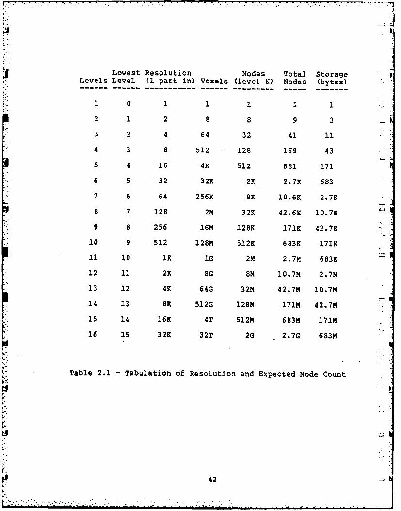
In Table 2.1 a number of items have been tabulated as a
function of the number of levels in the universe (assuming
the whole universe is the active workspace). The second
column is the level number of the lowest level. Column 3 is
* the resolution of the universe. In a universe with 111 levels, for example, the edge of the smallest obel is 1/1024
L 41
T' I, i". ,-.,i". ? :: "-: "-,"i <. i .- .,.,,.,,...,+ . ,,., ., .., ,, .,., , ,.,,.==._, . . .__ , 4
Lowest Resolution Nodes Total Storage 0Levels Level (U part in) Voxels (level N) Nodes (bytes)-------------------------------------------------
1 011111
2 1 2 8 8 9 3
3 2 4 64 32 41 11
4 3 8 512 128 169 43
5 4 16 4K 512 681 171
6 5 32 32K 2K 2.7K 683
7 6 64 256K 8K 10.6K 2.7K
8 7 128 2M 32K 42.6K 10.7K
9 8 256 16M 128K 171K 42.7K
10 9 512 128M 512K 683K 171K
11 10 1K IG 2M 2.7M 683K
12 11 2K 8G 8m 10.7M 2.7M
13 12 4K 64G 32M 42.7M 10.7M
14 13 8K 512G 128M 171M' 42.7M
15 14 16K 4T 512M 683M 171M
16 15 32K 32T 2G -2.7G 683M
Table 2.1 -Tabulation of Resolution and Expected Node Count
42

of the edge of the universe. The next column lists the
number of voxels (lowest-level obels) in the universe. This
is the number of storage locations required in a spatial
enumeration representation.
-- The fifth column lists the expected number of nodes at 5
the lowest level assuming that one-half of the children of.-." branch nodes are also branch nodes.
The sixth column is the accumulated number of nodes (C). -
It should be emphasized that this value is a rough estimate
based on simplistic assumptions. The object must be of
comparable size as the universe. In a much larger universe,
the C values can be thought of as applying to objects encoded
to a resolution relative to the object of approximately the
value given in the third column. Also, uniform resolution is
not required over the entire surface of an object. Given a
constant value of C, lower resolution over some sections will
.. allow higher resolution in other sections.
The last column is the storage requirement for the
object, sequentially allocated at 2 bits/node.
Given this information, what level of performance can be
expected from a specialized octree processor? It will be
-: assumed that a single unit could process a node in 50 nsec.
to 100 nsec., depending on the algorithm and function. If 30
- complete operations per second are required for real-time
operation, an object with a C value between 325K and 650KL
nodes could be handled by a single processor. According to
43

the table# this corresponds to an object defined over a
section of the universe of a size between 2563 and 5122.
Based on this admittedly crude analysis, for algorithms which
could be operated in parallel such as display, an 8-processor-
system would seem to be able easily to handle objects with an
average resolution of 1 part in 1024 in each dimension at
real-time rates. This assumes a single object in a-
worst-case situation Call nodes accessed). Such a system
would seem to be sufficiently powerful for most interactive
situations. More complex situations could be handled at a
slower rate.
The overall growth of C with resolution places an upper
limit on object precision in any practical situation. In
many cases performance could be enhanced if high resolution
was maintained only on surfaces where it was actually needed.
Nevertheless, many applications require much greater
precision than would be practical for a simple octree system.
To accommodate such situations, a dual data structure
approach is envisioned. -A specialized -data structure
*tailored for a specific application and its functional
requirements would be used in conjunction with a general
purpose octree-i,'..ed system. This latter section would
handle interactive geometric and geometry-related functions
such as object manipulation, analysis and display.
Items in the application data structure would be-
relatively permanent whereas the octree data could be more or
44

J6
less transient. This is somewhat analogous to the relation
Snbetween a conventional 2-D geometric data base and the frame
buffer memory of a raster graphics display. The description
of a circle in the data base may be an actual part of a
design while its representation in the frame buffer memory
would be temporary data generated to fulfill a specific need
-* such as visualization by the user.
Of course, frame buffer type data may be made part of
* the application data base. This could include the
digitization of a real-world image or perhaps a scene that
would be difficult or very time-consuming to recreate. In
like manner, octrees acquired from CT scanners or the final
results of a design session could be retained in theapplication data base in octree format.
* " The overall strategy is as follows. Objects or parts of
objects not maintained in octree format are converted from
user format beginning at the root and continuing down as
needed by the currently running processors on a demand basis.
In practice,. all items involved in a user session are kept in
octree format to some modest depth. This would typically be
the local depth at which each obel would contain only one or
very few primitives from the application data base. This
- corresponds to the locally optimal grid size in the
variable-grid technique of Franklin [21].
Sufficient information is kept with the current leaf
nodes quickly to generate the subtrees when needed. They are
L 45
soon discarded when their usefulness has passed.
What is to prevent the generation of all nodes to a low ..
level whenever a user makes a request? The answer is to
develop algorithms that require computation (request nodes)
in a quantity relate6 (in some sense) to the complexity of
the immediate situation rather than the number of and
complexity of all objects involved. In interference
detection, for example, the number of nodes examined could be
a function of the nearness of the objects. In hidden-surface
display, the computation could be related to the actual
complexity of the scene generated. The development of such
algorithms was a major part of this research.
L 46
L.

CHAPTER 3
OCTREE GENERATION
In addition to octree generation, an objective of this
chapter is to begin developing a body of "tools" to be
employed by algorithm& for performing sub-functions within
the implementation constraints (simple arithmetic, easy VLSI
implementation, etc.). This will be a "bag of tricks" from
which specific solutions will be drawn as the need arises.
These tools perform specific, not general, functions but
* .will, hopefully, be broadly useful over many algorithms.
Lower-level tools will be combined to form higher-level ones
Uto implement more sophisticated functions. At the lowest
level, tools are the simple arithmetic operators. To the
system implementor they correspond to specific hardware
* subsystems to be used in the construction of special-purpose
hardware processors.
In order to motivate the tool development, it will be
placed within the context of solutions to increasingly
difficult modeling system functions. In most cases,
solutions to the 2-D (or l-D) problem will be presented first
for clarity, followed by the extension to 3-D.
SL
47
-
• ..... . , ...- . . . .. . . . . . . . . .. . - . . ... . ° . . . . , ., . . , : - -:_
p'
3.1 Algorithm Considerations
Many factors were considered during algorithm design and
development. A few of the major ones will now be discussed.
The mathematical operations that algorithms can employ
are severely restricted because of speed, cost,
implementation and simplicity considerations. The permitted
("legal") operations are integer addition andsubtraction,
magnitude comparison, shifts, and data movements such as
LOAD, STORE, stack PUSH, stack POP, queue INSERT, and queue
DELETE. These legal operations form a set called simple
arithmetic.
Solid modeling.functions can still be performed, in
spite of these restrictions, because of the design of the
data structure. In almost all cases where a product (or
quotient) is needed, one of the factors is a power of 2. The
desired result can thus be generated by the process of
shifting.
Two phases of algorithm-operation are -defined: setup
and run. During the setup phase, a small number of
unrestricted computations are allowed for processing user
requests. During the run phase, the requested solid modeling -
function is performed over the octree objects. Only simple
arithmetic is allowed. In mass property measurement, an
isolated multiplication or division may be needed to compute
an intermediate or final property value.
48
*. . . . . . . . . . .
" . ." - . "-.." " '- --
During algorithm design, maximum advantage was taken of
I! the more or less standard techniques that have proved to
enhance performance. This includes extensive use of
parallelism and pipelining, avoidance of iteration, looping
or unbounded situations, and so on. The classical
computation-versus-memory tradeoff was generally decided in
* favor of extensive use of memory.
For most of the algorithms, two catagories of tree
traversal sequences, depth-first and breadth-first, are
possible. They correspond to two strategies for attacking
problems. A depth-first algorithm generally traverses a tree
downward from parent to child, returning to the parent when
-iall lower nodes have been processed. Breadth-first traversal
processes all nodes at one level before working the next
lower level.
Depth-firSt traversal tends to be used when local
information is required whereas breadth-first is employed
when global information is needed. Depth-first operations
typically use a stack, either directly or via reentrant code,
to maintain tree location. Breadth-first information is
passed from one level to the next in a queue.
494
,49-.a-o.

3.2 Octree Generators
It is expected that high-speed conversion from various
high-level application formats into octrees will be required.
Perhaps the most obvious method for this is the brute force
use of spatial enumeration. A full tree is first constructed
with all possible leaf nodes at the desired lowest level.
The input objects are processed with the leaf nodes
corresponding to the interior voxels marked F. As noted by
Requicha [56], conversion from any popular SMS format to
spatial enumeration is straightforward. The tree is then
simply reduced.
The obvious difficulty with this procedure is the huge -
memory requirement (O(8n ) where n is the lowest level) and
the associated processing time (all leaves must be accessed
at least once).
A variation is to generate 2-D quadtrees representing
orthogonal slices through the universe. They are converted
Fto an octree (voxels on a plane) and then ufnioned together.
All possible obels in the universe are still accessed but the
memory required may be substantially reduced. This method
was used to generate the medical octree objects from 2-D CT
images shown in Figures 7.2 and 7.3.
In some situations the bottom-up conversion methods of
Samet (68, 693 for quadtrees can be used. For the most
efficient cases, the computations can be proportional to
50

object complexity. This runs counter, however, to the
general strategy of converting from application format to
octree format in a top-down manner on a demand basis. Better
methods are needed.
-- A proposed solution is the use of specialized software
or hardware processors called octree Qenerators. As shown in
Figure 3.1 these would be preloaded with the object
parameters. The user of the data (the octree processor)
would request node values. The generator maintains the state
of the traversal in an associated stack or queue.
From a complexity viewpoint, the efficiency of an octree
generator is a function of the false rate. This is the
fraction of nodes marked P that will have a value of E or F
after reduction. This is not considered to be an error
because the obel has not been incorrectly determined. The
calculation of the final value has simply been postponed,
requiring additional work.
If the false-P rate is zero, all nodes are correctly
determined the first time -and the tree is-identical to the
reduced tree. If the obel values can be determined in
constant time, the computations grow linearly with object
complexity (C). If, for a typical user request, only parts
of a tree are needed, computations could be expected to be
linear (in some sense) in the complexity of the specific
case.
Conceptually, an unsorted input object can be converted
51
. ...

- --
Node Request/Response
Octree Octree StackProcessor Generator or
Queue
Preload(Object Parameters andTraversal Information)
Figure 3.1 Octree Generator
52
:;.. . .. . ... .. .. .. .. .. . .. . . .. .. ... .. .. ....
into a sorted octree in linear time, rather than O(n log (n))
U or worse time, because a radix-type sort over a finite
- alphabet" (the obel locations) is involved [1]. The worse
than linear growth of typical sorting operations is caused
when comparisons between elements is required. None are
required here.
The basic octree generation operation is to compare a
test obel and the real object being converted. The result is
one of the three status values, E if Obel f Object = 0, F if
* Obel n Object = Obel, or P otherwise.
The octree generation strategy is as follows. Beginning
with the root node the values of test obels in the output
octree object are determined by comparison with the input
(real) object. A node in the octree is created with this
* value. In most situations of interest this can be performed
in constant time. E and F nodes are terminal and need no
longer be considered. P nodes are subdivided with the
"* corresponding children used as later test obels.
The first algorithm tool to be- deviloped is the
calculation of child vertex coordinates from the parent
- values. As shown in Figure 3.2 for 2-D, this is easily
accomplished by means of additions and shifts (divide by 2).
*- The 3-D or N-D equivalent is obvious.
The following sections discuss the conversion of convex
L objects. Conversion of concave objects is much more
difficult and less well understood. Suggested approaches are
53

xO~xl YO-I
02 2y
OYl
Parent yo+yl
Yo0 1-2 --- V '
I 'Y)Y
xo 0l X 0 x 01 x I
(a) Parent (b) Children
Figure 3.2 Calculation of Child Vertex Coordinates from Parent Values.
54 -
7 7 7- 7 7 7- -7 7 - 7 _ .. ..
outlined in [431..p
3.3 Orthogonal Blocks
The development of object generation tools will begin
with a simple case, a 3-D block (rectangular parallelepiped)
%. with faces perpendicular to the major axes.
A typical case is illustrated in Figure 3.3. The
minimum and maximum coordinates in each dimension are noted.
Three test obels with the three status values are shown.
Because the bounding planes and axes are orthogonal, the
-.status determination can be decomposed into an independent
n comparison in each dimension. Determining of obel status is
straightforward.
The development and analysis of the orthogonal block
* generation algorithm is presented in (43]. It has a zero
false-P rate.
3.4 Convex--Obiects
The generation of octrees for convex objects is more
difficult than for blocks because the dimensions cannot, in
general, be analyzed independently. The basic low-level
operation is determining whether a particular vertex point of
a test obel is interior or exterior to the object. If the
object is a convex polyhedron, the surface is described by a
L 55

yp
Test Obel #1 (No Intersection, Status=E)-
Test Obel #2 (Intersection butNot Enclosed, Status=P)-
y max Orthogonal
#3(Enclosed,
* -- -Status=F)
I Ymin
;4 x
zmi maxa
Figure 3.3 Octree Generation for 3-D Orthogonal Block
56

set of planar faces, each of the form:
Ax + ty + Cz + D 0 3-1)
-.i -Each plane divides the universe into two half-spaces.
The half-space containing the object will be called the
positive half-space; the other is the negative half-space.
For points not on the plane, (3-1) will evaluate to a
positive or negative value depending on the half-space.
A simple substitution of the coordinates of the vertex
point determines whether the location is on the plane or in
one of the half-spaces. Note that a positive evaluation
value does not necessarily indicate the positive half-space.
Also, a point in the positive half-space is not necessarily
* within the object. The face plane is the entire plane
whereas the face is a segment of the face plane.
Since multiplications are not allowed, the components of
i I(3-1) are calculated for obel vertices by averaging from the
parent components. A set of components for each vertex point
in each dimension for each plane would need to be maintained.
In 3-D this requires 24 values per plane.
Alternately, the signed perpendicular distance from the
vertices of the universe to the plane can be calculated from:
d - (Ax+By+Cz+D)/((AI+Bt+C2 ) (1/2)) (3-2)
The distance value for a new vertex in a child obel is
the average of the two parent vbrtices defining the edge
containing the new vertex. The sign of the distance
57

indicates the half-space. The new distances are calculated
as follows:
d = (DVAL(AND(CHILD,VERT))+DVAL(OR(CHILD,VERT)))/2 (3-3) -
where CHILD is the child number of the new obel, VERT is the
number of the desired vertex of the new obel and D_VAL(n) is
the distance of parent vertex number n. The AND and OR
functions perform bit-wise Boolean operations on the child
and vertex numbers in binary format.
For each plane, 8 values are used (one for each vertex).
In practice, only one distance value need be kept. The
remaining values can be generated by adding an offset from a
pre-computed table.
For a convex polyhedron, if a point is in the positive
. .half-space of all face planes, then it is interior to the
polyhedron. If it is in the negative half-plane of any face
plane, then it is exterior to the object. Otherwise, the
point lies on the surface of the object (on one or possibly
more faces). A surface point touches the object but is not
considered to be interior to the object.
Thus, for polyhedral objects, an obel vertex point can
V be determined to be interior," exterior or on the surface
using simple arithmetic without considering the location of
the faces on the face planes or the actual intersections of
face planes.
For convex objects defined by an analytic surface the
58. . . . . . . . . . *
p.'
location of the point relative to the object can often be
determined by evaluating the defining expression for the
surface.
- In 3-D, the most general second-degree equation is:
Ax +By+Cz+Dxy+Exz+Fyz+Gx+Hy+Iz+J=O (3-4)
Note that the terms have three formats, a constant times
a coordinate, a constant times the square of a coordinate and
a constant times the product of two different coordinates.
Generating the terms of the expression .for the vertices of a
child obel using simple arithmetic on parent values can be
accomplished as illustrated in Figure 3.4. In 3.4(a) Gx is
the product of coefficient G and the coordinate value for a
" * vertex (x). The value of Gx' is the product of G and a new
pcoordinate value x'), a vertex of one of the children. The
value of Gx' is desired as a simple function of Gx from the
parent. Because the distance value between the two
[-' coordinates (x'-x) is equal td an edge of an obel at that
level (e), the needed multiplication can be performed by
shifts (e is a power of 2). It is computed as follows:
Gx' - G(x+e) Gx+Ge Gx+G(2(m-n) ) (35)
where m is the level of the lowest level in the universe
(where e-l) and n is the level of the child obel. The first
term is the parent value and the second is a shift of the
constant G. Thus, a shift by m-n followed by an add
operation will be sufficient.
59° '4

Gx Gx'
k- child -W- child -W
K- parent -
(a) Given Gx, calculate Gx'
Ax2 Ax'2
Ax Ax'I I
2*(b) Given Ax and Ax ,calculate Ax' and Ax'2
3 3~4-Kx x2Kx 2
Kx Kx'
(c) Given Kx, Kx2 and Kx3 calculate Kx', Kx'2 and Kx'3
Dy'Dx y'I
DxDy Dx'DxyDxy
x x'
(d) Given Dx, Dy and Dxy, Calculate Dx', Dy',Dx'y and Dx'y'
Figure 3.4 Generation Terms for Child Obel from Parent Values
60
-~~ ~ ~ ~ - ---
In Figure 3.4(b) the value of Ax'2 is desired from Ax
and Ax'. The value of Ax' will be needed later and is
calculated as above. The Ax'" value can be evaluated by:
Ax, = A(x+e)2 = Ax2+2eAx+Ae 2
(m-n+1))x+ (2(m-n)Ax'+(2 )Ax+A(2 (3-6)
Two shift operations and two adds are required in
addition to the shift and add to compute Ax'.
More sophisticated objects involving third-order
equations require Kx'' as shown in Figure 3.4(c). The Kx'
and Kx'' values are maintained as above with Kx'' calculated
as follows:
Kx's = K(x+e)* = Kx3+2eKx2+e2Kx+eKx'+2e2Kx+Ke3
= Kx3+(2 (m-n+l))Kx2+(22 (m-n))Kx+(2(m-n))Kx'
+(2 (rn-n)+1) )Kx+(23 (r-n))K (3-7)
Five additional shifts and adds are used for a total of
8 each.
Two cross-product terms are illustrated in Figure
* 3.4(d), Dx'y and Dx'y'. The first is tomputed from the
parent values of Dx, Dy and Dxy as follows:
Dx'y - D(x+e)y = Dxy+eDy - Dxy+(2 (mn))Dy (3-8)
A shift and an add are needed. The second is computed
by:
Dx'y' - D(x+e)(y+e) - Dxy+eDy+eDx+e'D
61
=Dxy+(2(m-n) )Dy+(2(m-n))Dx+ (22 (ln) )D (3-9)
Three shifts and adds are needed.
Based on these tools, zero false-P algorithms for the
conversion of polyhedra and restricted objects defined
mathematically have been developed [43].
62

7 7i . .7 -7. ,70 77 -7 7- T -7,. .7% . - L - ° r -. " L . .°"-.
CHAPTER 4
ANALYSIS AND MANIPULATION
4.1 Object Properties
Of the following methods for object property
determination, volume, surface area and separation of
S,.disjoint parts are 3-D extensions of published quadtree
techniques [65, 66, 74].
4.1.1 Volume
Volume is the sum over all levels of the product of the
F node count and obel volume (a power of 2) at each level.
If an error tolerance is allowed, a minimum and maximum
volume can be calculated breadth-first from the root. Only F
nodes are summed into the- minumum while-P nodes are also
summed into the maximum. When the average is within limits,
processing is terminated.
f63
. -...
4.1.2 Surface Area
Surface area is simply the sum of the areas of all
exterior obel faces (faces separating an E node and an F
node). F nodes may need to be subdivided (if a face touchesboth E and F nodes).
4.1.3 Center of Mass
If a homogeneous object is divided into n disjoint -
regions having volumes Vl, V2 , ... Vn and centers of massUXlX 1" "1 , 0.-. (xI •0 n the"-
.1 o 1 x2,1X 2 ,n ' ** XN,n
object center of mass, (xx 2, ... xN) can be calculated as
follows:
n nx. i SUM(Vjx i )/SUM(V.) (4-1)
j= 1 j=l -
For an octree object, the disjoint regions are the F
nodes. The centers are the obel centers and the volumes the
obel volumes (a power of 2).
If a tolerance is allowed, a minimum and maximum can be
computed during traversal.
64 A4
ii
4.1.4 Moment of Inertia
The moment of inertia, I, is defined as follows:
nSSUM(MiRi2) (4-2)i=1
where Mi is the mass of particle i and Ri is the1
1
-. perpendicular distance to the axis of rotation.
For a homogeneous octree, the mass of an F node is
proportional to the volume (a power of 2). The distance
- - squared value is computed using simple arithmetic as shown in
the octree generation section, if the axis of rotation is (or
* has been made through rotation) parallel to a coordinate
system axis.
. T h The above formula assumes a point mass. Errors result
* if the center of a distributed mass is used. This is
corrected by employing the parallel-axis theorem. The number
of F nodes at a level is multiplied by the moment of inertia
for an F node (at that level) about a parallel axis through
* - the node center (a precomputed constant). The sum over all
levels is added to the result of (4-2) to determine the exact
value.
L
& -65
I . . . . . .. .. . . . , ... .. , . - . .. . • , . . • . .. . , . - . . - .. . ... .:
. . . . . .. . . . . . . . . . . a. . . . .
*1.- ,A
4.1.5 Segmentation of Disjoint Parts.4
The quadtree connected component labeling algorithm of
Samet [661 is easily extended into 3-D to separate disjoint
parts of an octree into multiple octrees.
4.1.6 Interior Voids
To obtain the number of interior voids the octree is
negated (see below) and segmented into disjoint parts. The
value is generally the number of parts minus one (the
exterior).
A space filling operation is performed if one or more of
the negated interior sections is unioned back into the
original object.
4.1.7 C.rrelatio
A measure of correlation between two objects is the
fraction of the containing volume having the same status (E
or F) in both objects. The containing volume is typically
the bounding box of the union of the objects. The
correlation can be expressed as follows:
(volume((A B) n BOX) + volume (A n B) )/volume (BOX) (4-3)
66
• ,' "-r ,",' ,, '. ' "- % ",, " • .• ' "' "' "" - " " .

.- 7
where A and B are the objects and BOX is the bounding box.
4.2 Set O2erations
The set operations are the 'regularized" operators [791.
Conveniently, this is the normal result of the quadtree and
octree operations.
Algorithms to perform the set operations of union,
intersection and difference have been published for quadtrees
by Hunter and Steiglitz [291 and are directly extendable to
3-D octrees.
Computation is linear in object complexity (proportional
to the sum of the C values for the input trees). Known
algorithms for CSG and B-Rep are worse than quadratic because
of the combinatorial explosion of face comparisons to detect
new edges (see (28], for example).
The negation operation is performed by simply changing
all F nodes to E and vice versa. Objects are sectioned by
subtracting a "blanking object* (typically a half-space
defined by a plane).
Figure 4.1 is an example. The set operations of union,
intersection and difference are performed on objects A and B,
resulting in three new octree objects.
67
. .., .-
....67

(a) Object A (b) Object B
(c) AUB8 (d)A n B (e) 8-A
Figure 4.1 Example of Octree Set Operations
68

-- r. -7 7 .
4, .
4.3 Overlays
One of the most important tools employed within octree
algorithms is the overlay. From an implementation viewpoint
its importance would be difficult to overstate.
An overlay is a set of contiguous nodes at a single
level, drawn from an input tree, such that the space it
represents is guaranteed to enclose the space of an
associated obel, the target obel, from another tree. The
second tree is usually an output object being generated. By
examining the overlay, a decision (perhaps an interim
decision) can be made as to the status of the target obel.
For example, in 3-D an overlay containing a set of 8
obels all of which touch at a common point will always
completely enclose a randomly located target obel of the same
size or smaller if orthogonally oriented (not rotated). The
record for each overlay obel may contain a pointer to a node
N.. in the input tree or the status value of an implied nodeN.°
taken from the terminal node ancestor.
The overlay can be thought of as a template containing a
number of obels which cover a section of space. Within an
overlay there is usually -a single obel in a fixed spatial
location (relative to the overlay) such that if the origin of
the target obel is within it, the target obel is covered by
the overlay. The shape of the overlay, the number of obels
69
it contains, the level of its obels relative to the level of
the target obel, etc. depend on the specific algorithm. PBy maintaining a set of active neighbors, the overhead
of having pointers chasing through the tree to examine
neighboring nodes is greatly reduced. From a computational -
growth viewpoint the savings are not significant because the
expected value of the average traversal length required to
locate a neighbor is a constant (66]. From an implementation
viewpoint, however, the savings can be substantial because
fewer memory references are needed.
Operating under the self-imposed restriction of using
only simple arithmetic, the strategy in several of the
algorithms below is to set up an output tree and then proceed
to examine its obels for spatial interference with the input
tree or trees. A status value based on the status of
intersecting nodes is given to the output node.
Simple CSG systems perform an interference test by
mathematically comparing the test primitive to each primitive
in the object. The number of comparisons is equal to the
number of primitives in the object.
Because of the spatially pre-sorted nature of the
octree, it is not necessary to'check all nodes in the input
tree for interference. Only those which can possibly
intersect the target obel, i.e., those in its overlay, are
tested. Thus, the total number of tests needed to generate Ik
an output object is limited to the product of a fixed,
70

-='-7,6 77
usually small, number (the number of nodes in an overlay) and
the final value of C for the output tree (before reduction).
Advantage cannot be taken of this technique in most
current SMSs because the primitives are not and usually
cannot be spatially pre-sorted.
Several tools are needed to evaluate the status of the
target obel. First, the overlay obels actually intersecting
the target must be determined. This can be a difficult
problem, depending on the algorithm.
Second, a status value must be determined. If all
intersecting nodes have the value F, the target is given an F
value. The same is done for E. Otherwise, the target is
subdivided and each child processed in like manner.
" iThird, a sub-overlay must be generated for a specific
child of the target. Each sub-overlay is identical in
structure to the parent overlay with the new overlay obels
being drawn from the set of children of the overlay obels.
Sub-overlay generation begins by determining the origin
of the new target. Since it must be within a specific
overlay obel, the exact enclosing child of the overlay is
determined. The selection of the remaining sub-overlay obels
S-.: is fixed by the structure.
711[-.1
'-'" 71
• . . _ .. . . . . . ... . .. . .. .. .. .•. . . .. .. .2

L7
4.4 Geometric Operations
For translation, scaling and rotation, the formal
procedures are in [391.
4.4.1 Translation
The translation algorithm converts an object and a
movement vector into a new tree representing the translated
object. The process begins by generating an augmented
overlay universe composed of the "old" universe containing
the original object and a number of empty universes put
together so that the "new" universe, which will contain the
translated object, is covered by the old universe. The
translation vector specifies the alignment.
Beginning with the root of the new universe, the new
tree is traversed and its node values generated by
simultaneously traversing the old tree using the overlay
technique outlined above. If a terminal node in the new tree
is generated, no descendants of that node need be considered.
If an ambiguity exists and the status cannot be resolved, a P
node is generated. Its children are produced in the same
manner.
The overlay obels can be at any level relative to the
target obel. The lower the level below the target, the more
numerous but more accurate the result (lower false-P rate).
72

The translation algorithm presented here uses an overlay with
2N obels at the same level as the corresponding new obel.
N Figure 4.2(a) illustrates a I-D overlay. The target has
an edge size of e. The overlay is made up of two adjacent
obels of the same size from the old universe connected at the
overlay center. The offset value is the distance from the
local origin (lower end of target) to the overlay center. It
is limited to 0<=offset<e. The equivalent in 2-D is shown in
Figure 4.2(b). The 8 overlay cubes and the target cube for
3-D translation are illustrated in Figure 4.3.
The orthogonal block techniques from the object
generation sections above are used to determine intersection.
S-. .The target obel corresponds to the convex object and the
- overlay obels correspond to the test obels. One difference
is that the target obel does not remain fixed for all time.
*o-" It subdivides. This presents no problem because the
point-to-edge or point-to-plane distance values are easily
updated for target subdivision using the techniques for test
obel subdivision. The edges and faces -of target obel
-_ children are parallel to the parent edges and faces.
-;. A detailed description of the translation algorithm is
given in [39].
An example is presented in Figure 4.4. An object and
the six obels forming it are shown in 4.4(a) and 4.4 ',
respectively. The new object in 4.4(c) was created by
L. performing a translation in z by half the wi3th of an obel.
73
. . . -*.. . . .. .. -.. . . . , . , . . . *. . . . . ,_ -
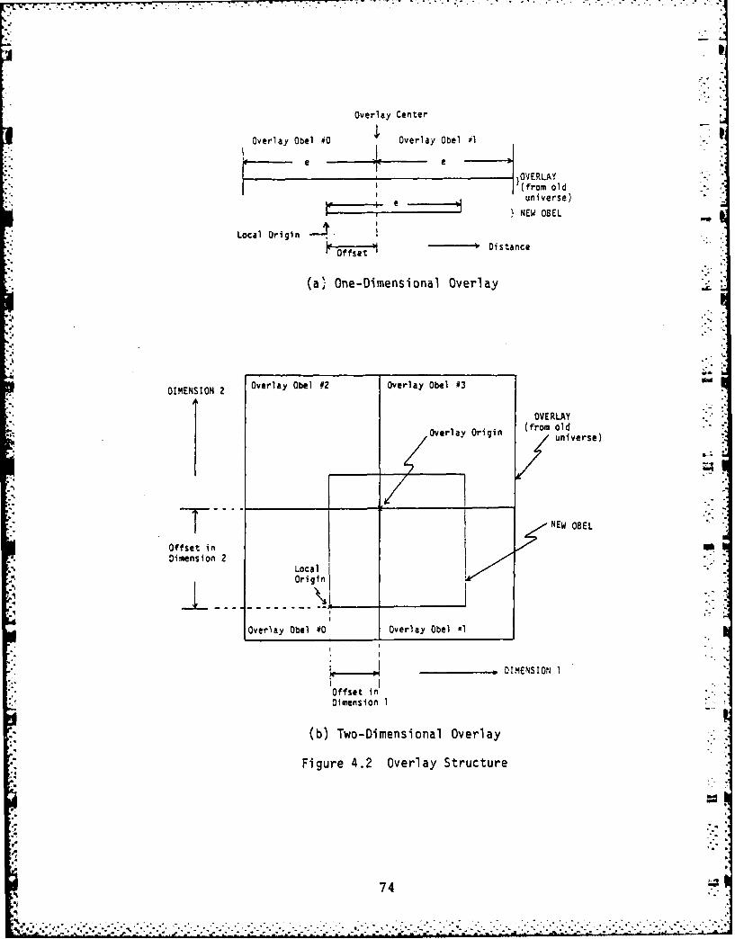
Overlay Center
Overlay Obel #0 Overlay Obel 01
e e -- ----)
~OVERLAY)(from olduni verse)
NEW OSEL
Local Origin -Offset Distance
(a) One-Dimensional Overlay
DIMENSION 2 Overlay Obel #2 Overlay Obel #3
OVERLAY(from old
Overlay Origin universe)
T NEW OBEL
Offset inDimension 2
LcalOigin
Overlay Obel 00 Overlay Obel *I
____________DIMENSION I
Dimension I
(b) Two-Dimensional Overlay
Figure 4.2 Overlay Structure
74
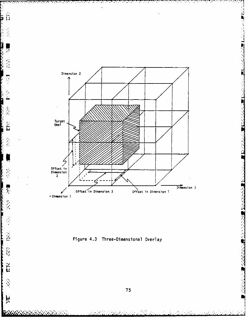
Dimension2
* - Target* Obel
Ld
k .A
Ofse i
Dimens75
U ~ . *. % * * . .. . . . .. . . . . . . . . . . . . . . . . . . . . .

(b) Object Obel s
(c) Translated Object
Figure 4.4 Example of Octree Translation
76
Note that each end is now formed by four obels from the next
lower level.
4.4.2 Scaling
'. Scaling an object by a power of two in all dimensions is
accomplished by adding or deleting levels at the root. An
object is halved in each dimension by adding one level at the
top. The new root points to one branch node, the old root,
and 2N-I empty terminal nodes.
In like manner, selecting one of the first-level nodes
to be a new root doubles the size of everything within it.
For an arbitrary section of space, it is translated into a
n first-level obel and then expanded to fill the universe.
Objects can be expanded or reduced by any power of 2 by, in
- effect, repeated expansion or reduction.
. Scaling by a factor other than a power of 2 is
accomplished using an overlay scheme similar to that used for
- translation. The target obel, however, may be smaller than
the overlay in one or more dimensions. In addition, a single
°-i set of offset values cannot be used. The local offset vector
must be computed independently fo'r each child of the target
obel. A detailed description is presented in [39].
Figure 4.5 shows an object scaled by a factor of 1.75 in
the y direction. The original object is in 4.5(a) and the
new object in 4.5(b). In 4.5(c) the additional obels are
77
. * . . .
-" * " , " ",.. . . ". ". , . , .. .. . . ...- '. . . . . . . .. • " . . . . . ,. , o.. ..

(a) Object bels
(b) Scaled Object
(c) Obels of Scaled Object
Figure 4.5 Example of Octree Scaling
78
, 'visible.
- 4.4.3 Rotation
Rotation by 90 degrees about an axis can be performed by
"" a simple reordering of the nodes in the tree. For an octree,
if the center of rotation is the center of the universe,
, rotation by 90, 180 or 270 degrees or reflection across a
-* plane through the center parallel to a face of the universe
or oriented at 45 degrees is accomplished by reordering or,
u within an algorithm, a change in the traversal sequence.
Figure 4.6 is an example of an object and two new
versions rotated by 90 degrees using this method.
For rotation about an arbitrary point, the object can be
translated to the center of the universe, rotated, and
translated back.
Rotation by an arbitrary angle is more difficult. In
2-D, the overlay arrangement for a 0 to 90 degree rotation is
shown in Figure 4.7. Nine.overlay obels are required. The
local origin of the target obel is always in overlay obel B.
Clearly, for 0 deg. to 90 deg. rotation, the target will be
* covered by the overlay in dimension 1. In dimension 2, the
maximum reach of the target is I + SQRT(2) which is less than
3, the height of the overlay. Coverage is thus guaranteed.
Again, the techniques from the object generation
sections are used to determine overlay obel intersection. A
p.7
79
* .. . . .... . . . . . . . .-

Object Rotated about
Rota ted IS* About
x-axi s
Figure 4.6 Example of Octree Rotation by 900
80 k
4L.1."- .

G -
Target Obel.
Local Origin of Target
* -Local Origin of Overlay
Figure 4.7 Rotation Overlay
81
detailed description of the algorithm is given in (391.
For an arbitrary 3-D object rotation, three operations
could be performed using a slightly modified 2-D algorithm,
one for each axis. An even simpler method is to perform
multiple skew operations. Iftikhar [321 has proposed this
based on the 2-D work of Catmull and Smith (151. This
approach may be generally undesirable, however, because at
the lowest levels aliasing products are generated on the
object surface when nodes are forced to be terminal. The
object is essentially being redigitized from a previously
digitized object. This tends to corrupt the surface and is
compounded by the repeated operations that are required.
This is minimized by computing nodes to lower levels, by
performing operations in a single pass and by regenerating
instances of an object from the original octree model each
time it is moved or changed (rather than incremental movement
of a single object).
Because of this, 3-D rotation in one pass is preferred.
* This is accomplished by extending the 2-D scheme into 3-D by &
the use of a 4 by 4 by 4 overlay. As shown in (431, a 3 obel
per edge overlay is not sufficient.
Figure 4.8 is an example of rotation by an arbitrary
angle. The six-obel object from Figure 4.6 has been rotated
by an angle selected at random (28.7 degrees). In 4.8(a),
obels are forced to be terminal at the same level as the
obels in the original object. In the algorithm used, all P
82
~ t .... . * s..Ct.C titItXCLC S ~t< C 2 2 a.. .... .. - .., S- . ~ .t .
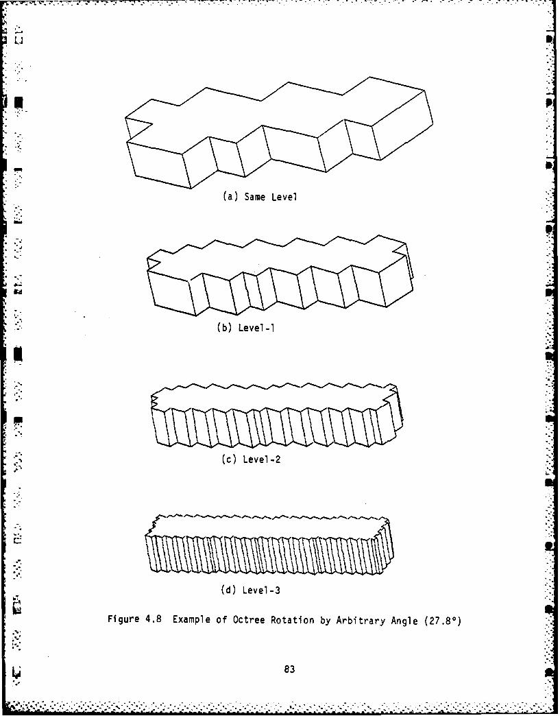
(a) same Level
(b) Level-i
(c) Level-2
(d) Level-3
Figure 4.8 Example of Octree Rotation by Arbitrary Angle (27.80)
83

nodes at the lowest level are given the value F, causing an
enlargement of the object. In 4.8(b) through (d), -
increasingly lower levels are used, allowing a higher
precision result.
4.4.4 Concatenated Geometric Operations
Using homogeneous coordinates [48] any number of
sequential linear operations (x' = Alx + Bly + CI, y' = A2x +
B2y + C2) can be concatenated and reduced to a single matrix
of coefficients (3 by 3 for 2-D or 4 by 4 for 3-D). This, of
course, includes the geometric operations of translation,
scaling, rotation and skewing. The composite transformation
can then be performed in a single matrix multiplication. The
correlation can be expressed as follows for 2-D:
[A A20[xI,yl,l] = Ex,y,l] B1 B2 (4-4)
C I C2 J
Reversing for the moment the direction of data flow in
an overlay operation (the target obel will now "generate" the
overlay), the above concatenated transformation will be
performed if a parallelogram-shaped target obel is used as
shown in Figure 4.9. The target universe is assumed to be of
unit edge length. The matrix coefficients determine its
location, orientation and shape.
The C coefficients specify the location of the origin of
the universe. The A coefficients determine the length and
84
'- % L...7 V

B B
Figure 4.9 Target Obel for Concatenated Geometric.4 4...T
r a n s f o r m a t i o n
85
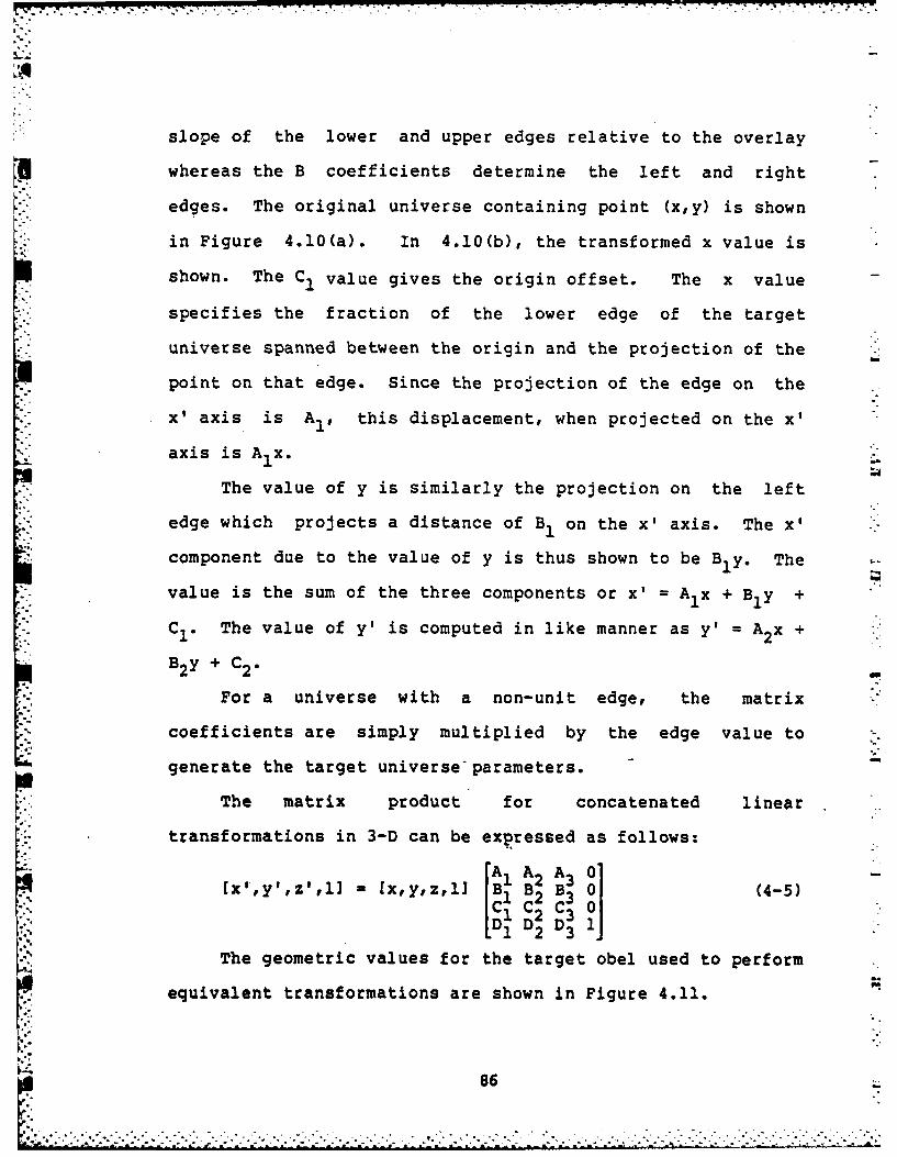
slope of the lower and upper edges relative to the overlay
whereas the B coefficients determine the left and right
edges. The original universe containing point (x,y) is shown
in Figure 4.10(a). In 4.10(b), the transformed x value is
shown. The C1 value gives the origin offset. The x value
specifies the fraction of the lower edge of the target
universe spanned between the origin and the projection of the
point on that edge. Since the projection of the edge on the
x' axis is A,, this displacement, when projected on the x'
axis is Alx.
The value of y is similarly the projection on the left
edge which projects a distance of B1 on the x' axis. The x
component due to the value of y is thus shown to be Bly. The
value is the sum of the three components or x' = A1x + Bly +
CI. The value of y' is computed in like manner as y' = A2x +
B2Y + C2.
For a universe with a non-unit edge, the matrix
coefficients are simply multiplied by the edge value to
generate the target universe parameters.
The matrix product for concatenated linear
transformations in 3-D can be expressed as follows:
A1 A2 A 01[x',y',z',l] - [x,y,z,l] BI B2 B3 0 (4-5)
C C2 C3 0[D1 D D 1
The geometric values for the target obel used to perform
equivalent transformations are shown in Figure 4.11. 01!
86
THE DCTREF ENCODING METHOD FOR EFFICIENT SOLID MODELING 2/2
(U) RENSSELAER POLYTECHNIC INST TROY NY IMAGEPROCESSING LAB D J MEAGHER AUG 82 IFL-TR-032
UNCLSSIFIED N 4-82-K-0 FG 9/2 NL
II.,lII~l,llllllIllllll
NO///Wn/l

. 0 JA I. 1 2 2 & .
W.0
.... 11.0
111.25 IILA *j~• M
MICROCOPY RESOLUTION TEST CHART
NATIONAL BUREAU OF STANDARDS-1963-A
5
.555. . ..=-. - -..... 5-- ..

LI
y ---- (x,y)
01
(a) Universe Before Transformation
Ounivers
B y
Origin ol
I I I .. xin
B~y 1
K -x'=A 1x+Bly+C 1
(b) Generation of Transformed x Value
Figure 4.10 Transformed Coordinate Value
87L

Projection of Target Obel
I..B
*~ LI
() Projection of Target Obel on xl'-Z Plane
F~gue 411 argt Obl fr 3D Cncatnatd Gomeric Tanratone
C8
3.*~C>K- --- ~
Returning to the original data flow from overlay to
target obel, the new obel is generated from the overlay when
it is deformed according to the inverse of the coefficient
matrix.
The distance values needed to determine overlap can be
updated using previous techniques because the edges and faces
" . of the children are parallel to those of the parent.
Mb -If the relative tree level difference between the target
.-- and overlay is fixed, the number and arrangement of overlay
obels cannot be fixed unless restrictions are placed on the
matrix coefficients. An alternate strategy is to fix the
overlay configuration and subdivide the target obel at
algorithm initialization until coverage is guaranteed.
*! If the shape of the target obel is generalized (not
restricted to a parallelogram) nonlinear transformations such
as perspective deformation can be performed [431.
-9
I-
89_
':
-. *. * -... * *"

-. 11N77K -74 7n
CHAPTER 5
INTERFERENCE ANALYSIS
5.1 Interference Detection
Interference detection as used in this section is the
detection of a situation in which the proposed insertion of a
-0new" 3-D object into a workspace at a specific location
would cause it to occupy space already occupied by an
existing "old" object or objects. It may be sufficient
simply to determine that an interference exists. In other
cases, the actual spatial interference 'object" may need to
be computed.
For a practical system, two primitive operations are
required, object insertion (including interference detection)
and object deletion. Additional operations could be defined.
An interference universe is maintained -in which large
numbers of objects can be inserted and deleted efficiently.
Since it can be assumed that some objects will be very
complex, it would be very desirable for the required
computations to be related to situation complexity, not
object complexity.
Conventional interference detection as performed by
existing SMSs takes the following form [801: A
90 *

*n
)..i nOBJECT.)UNION (NEW-OBJECT n OBJECT (5-1)i-i I
I where NEW-OBJECT is the object to be inserted, OBJECTi is the
i-th object already in the interference universe and n is the
number of objects.
* Clearly, such a procedure could require a processing
time proportional to the product of the complexity of the new
object and the complexity of all existing objects in the
universe.
For schemes such as CSG and B-Rep, the unioning of all
existing objects into a single object for testing would
probably not reduce the problem because most if not all of
the primitives would typically be retained. In any event, if
some method were used to reduce the primitive count, the
deletion problem would become more difficult. The subtree
corresponding to a particular object could no longer be
simply deleted.
The use of a binary tree to detect the intersection of
orthogonal rectangles has been reported by Bentley and Wood
[51. Briefly, a 1-D hierarchical "segment tree" is
:- maintained for the width of rectangles while the universe is
scanned in height. The sorted data format of the segment
• tree is shown to allow insertion and deletion in log time.
The spatially pre-sorted nature of the octree will now be
used to facilitate 3-D interference detection.
I. Two data structures are defined, an object table and an
91
_*°r' ':.-...-'."...-'-',":.,".'-..'. -.. '. -"-'- - :..:;,? ? :--,::'. ::% '. .,:I;':' :-",-,: -::: "-:: : ', : -- :-:?: :.4
octree interference universe. The object table will be
indexed by object number, a transient number assigned to
objects. Table information will identify the object, point
to the tree location in memory, etc.
It will be assumed that all trees will be reduced.
Trees with false-Ps could be used with slightly modified
algorithms but efficiency would be reduced.
The interference universe must be configured such that
objects can be distinguished at the obel level.. Each node
maintains a list of. records. They contain the object numbers
r',MN -A
of interference objects having P or F nodes corresponding to
the interference universe node and associated information
such as tree pointers. P node records will be marked as -
ecs T or unexpanded. They are expanded if their children
are also contained in the interference universe. If their
children have not yet been added to the lists attached to
lower nodes in the interference universe, they are unexpanded
nodes.
Nodes of the new object, are inserted -in a generally
breadth-first traversal. The state of node insertion is
Ssaved in a queue. If an input P or F node is inserted into
an interference node containing no objects (the list is
empty), no interference can exist at this node or below. it
is not expanded into lower levels.
if an input P node hits an PF node or an input F node
hits a P node in the tree, an interference has been detected
92 J
":' hilren avenotyet eenaddd totheliss atachd t

(all trees are reduced). If all nodes are P, they are
expanded. This continues until an intersection is found or
all potential interference nodes are expanded. The depth of
the descent and, therefore, thenumber of nodes expanded is
related to the nearness of the possible interference objects
over the surface of the input object.
Deletion is performed by traversing the object's octree
and deleting its records from the node lists.
A major problem is the expansion of memory to hold the
interference universe. It could expand to eventually
approach the sum of the C values for all objects. The vast
bulk of the nodes would have been expanded in an ad hoc
manner to detect specific close approaches; the probability
that most would ever be used again would generally be low.
Obviously a Ogarbage collectionu function is required to
delete unneeded interference nodes and their lists. From the
lowest levels, nodes would be deleted from the lists and the
parent entry changed from expanded to unexpanded. Assuming
node expansion is relatively costly in time,, and insertions
are not completely random in location, it would be
advantageous not to perform this operation after every
insertion. Spatially close inserts later may be able to take
advantage of earlier expansions. An asynchronous processI~ii would perform the garbage collection based on depth and time
since last use, similar to a cache memory in a conventional
mainframe computer. User requests would, of course, take
93
I.-.i
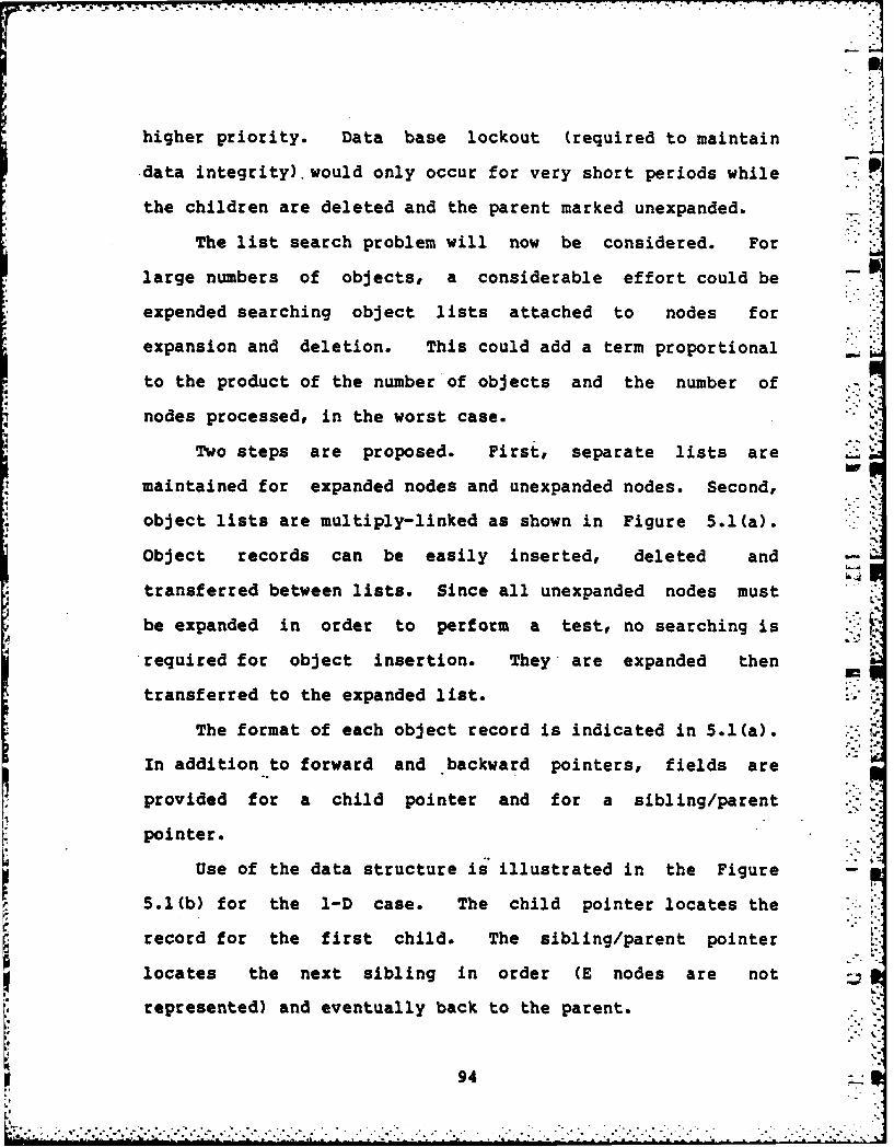
higher priority. Data base lockout (required to maintain
data integrity).would only occur for very short periods while
the children are deleted and the parent marked unexpanded.
The list search problem will now be considered. For
large numbers of objects, a considerable effort could be -
expended searching object lists attached to nodes for
expansion and deletion. This could add a term proportional
to the product of the number of objects and the number of
nodes processed, in the worst case.
Two steps are proposed. First, separate lists are
maintained for expanded nodes and unexpanded nodes. Second,
object lists are multiply-linked as shown in Figure 5.1(a).
Object records can be easily inserted, deleted and
transferred between lists. Since all unexpanded nodes must
be expanded in order to perform a test, no searching is
required for object insertion. They are expanded then
transferred to the expanded list.
The format of each object record is indicated in 5.1(a).
In addition to forward and backward pointers, fields are
provided for a child pointer and for a sibling/parent
pointer.
Use of the data structure is illustrated in the Figure
5.1(b) for the 1-D case. The child pointer locates the
record for the first child. The sibling/parent pointer
locates the next sibling in order (E nodes are not -.
represented) and eventually back to the parent.
94 .5

4
Level n Interference Universe Node Level n
* List Pointer
Obec Obec Jc
BakadCia.iligPrn owr
~~~.,~~~T ObBcwrdjCidSiln/a et SibForward
BFrom Obt Parent Rcr
Level nl Nodle Lee ]lNd- ~ .. j Level nl
L Lel nde Levelre nevl nde hlde
()Child and Sibling/Parent Links
Li Figure 5.1 Interference Detection Universe Pointers
95
These pointers can be used for garbage collection.
First the data base is locked.. The lowest level, lowest Z71
numbered child is selected. It and its siblings are deleted.
The parent is then marked unexpanded and the data base
released.
For deletion, the object table entry for the object is
marked inactive. For each record processed, the table would A
be checked. If inactive, it would be ignored. In a
specialized processor, this could probably be performed
transparently with little loss of performance. Anm
asynchronous process would then proceed to delete the
object's records. When done, the object number is released
for future use.
For insertion, if only expanded nodes are allowed or if
no unexpanded nodes are encountered, the computations will be
proportional to the number of input nodes that required
processing. This number is related to situation complexity.
The worst case would require the processing of a number of
nodes equal to about C for the input object. The minimum
would require almost no computation. For example, inserting
a complex object into an empty octant of the universe would
require negligible work even if the other octants contained
objects of great complexity. If unexpanded nodes are
encountered, expansions equal to C times the number of
objects ci be ,ed to-obtain an upper bound.
The lcwest level at which nodes need be tested can be
96

7% Z.. .7 r
determined if no intersection is found. For two objects to
occupy some part of the same obel, they must be within
SQRT(3) times the edge size of the obel. Thus, the lowest
." possible level will be:
n 10g 2 (SORT(3)E/d) (5-2)
where E is the length of an edge of the universe and d is the
shortest distance between the two objects.
Based on the assumption of one-half branch nodes, thenodes tetdwol4e n+l 1l
* "-'expected number of nodes tested would be (2/3)4 -...
Empty nodes are included because they are accessed, even if
not processed.
These upper bounds are only reasonable if all nodes must
be divided down to the lowest level, that is, if the closest
distance of approach to another object existed over the
entire surface of the object.
If the object surface area in the vicinity of the point
of closest approach is small and this distance is small
compared to the equivalent distance over the remainder of the
object, one"could expect that, below a certain level, few
branches would continue from one level to the next lower
level.
If no interference is found, no conclusion, can be drawn
concerning the minimum distance of separation. In fact, the
objects could be touching.
If a safety margin is needed around an object,
97

region-growing techniques could be employed or two
interference universes could be maintained and tested, one
having a coordinate system offset relative to the other.
The technique can also be used with hexadecatrees for
kinematic analysis.
5.2 Swept Volume -
In applications such as the verification of NC
programming, collision avoidance and trajectory planning in
robotics systems, interference analysis involves the "object"
swept out by an object in motion.
Two algorithms have been developed for swept-volume
determination. The first is the "translation" swept-volume
algorithm. It generates the swept volume for an object
translated in space while maintained in a fixed orientation.
It is presented below. In the second, the "rotational"
swept-volume algorithm, the object is rotated in a fixed body
movement about a line in space parallel to an axis. It is
described in [431.
The translational swept-volume algorithm accepts an
octree and a curve in space (represented by a chain code)
then generates the swept octree object.
98
. - -I lI IIII I! I . .........- * ~ ?.' in

- .'- 5.2.1 Convolution Formulation of Swept Volume
In image processing, a 2-D convolution summation [14,
60] such as the following is often employed:
k mv(k,m) = SUM SUM u(i,j)h(k-i,m-j) (5-3)
i=O j=0
where u is the input, h is the 2-D weighting function and v
is the output.
In (5-3) h(k-i,m-j) is the weight at the location k-i
units in the negative x direction and m-j units in the
negative y direction from the output point being considered,
"-- .(k,m). This corresponds to a point i,j from the origin and
. is therefore multiplied by u(i,j).
The translational swept-volume operation can be
formulated in terms of a convolution operation. Again for
simplicity, 2-D swept areas rather than 3-D volumes will be
n considered. The result is easily applied to 3 or more
dimensions.
First the non-hierarchical situation will be examined.
The input is a binary 2-D object contained in a spatial
enumeration array (not a hierarchical tree). An E value
indicates exterior and an F value, interior. The weighting
sequence will be a similar array with an F value at each
- location that would be visited by the square at location 0,0
if stepped along the sweep path. All other weightings are
zero.
99
Lo . -.. ... . . . . . .. . . .. . , . . . ' . .
A ;7.
The (5-3) convolution formulation is rooted in the 1-D
processing of functions of time. The weighting sequence is
defined from time 0 in a positive time direction. In two and
three dimensions, such directional distinctions seldom exist.
In order to be consistent with previous usage, universe
coordinate values will be kept positive. This requires that
the above sense of direction be reversed. Objects will be
swept along a path that is entirely within the quadrant
containing negative coordinates relative to the origin. The
index values i and j will thus run from k and m,
respectively, to n, the highest array index. In a real
system, of course, the summation index would be expanded to
handle both positive and negative coordinates.
In the swept-area case, the sum from (5-3) indicate the
number of steps along the path for which the location was
occupied but is typically a useless piece of information. A
single occupancy of the location is sufficient. Thus, the
binary input and binary weighting functions can be processed
by the following version of convolution .(F = TRUE, E =
FALSE):
n nv(k,m) - OR OR AND(u(i,j),h(k-i,m-j)) (5-4)
i=k j=m
In operation, the calculation can be terminated when the
first true value (occupancy) has been found.
100 J
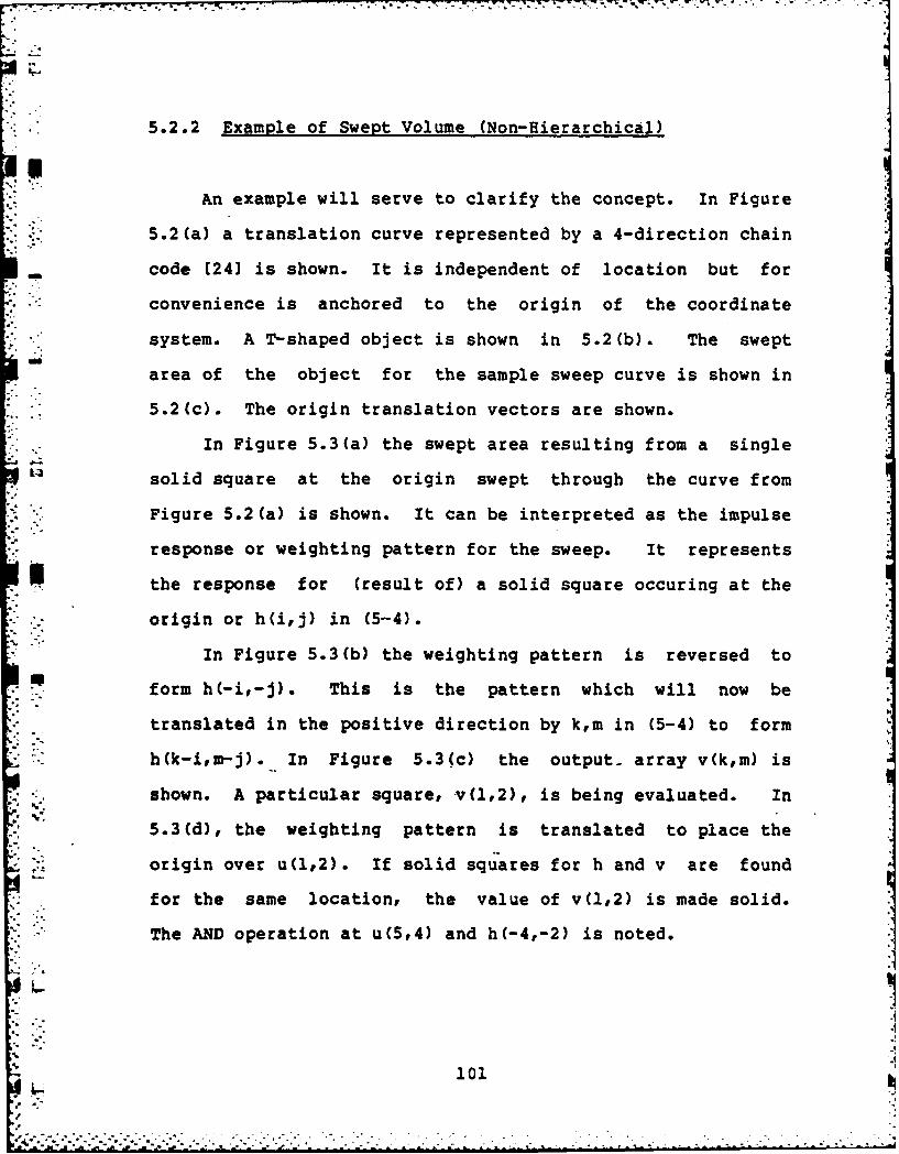
LI*.-.5.2.2 Example of Swept Volume (Non-Hierarchical)
An example will serve to clarify the concept. In Figure
5.2(a) a translation curve represented by a 4-direction chain
code [24] is shown. It is independent of location but for
, :convenience is anchored to the origin of the coordinate
system. A T-shaped object is shown in 5.2(b). The swept
area of the object for the sample sweep curve is shown in
5.2(c). The origin translation vectors are shown.
In Figure 5.3(a) the swept area resulting from a single
solid square at the origin swept through the curve from
Figure 5.2(a) is shown. It can be interpreted as the impulse
response or weighting pattern for the sweep. It represents
1. the response for (result of) a solid square occuring at the
origin or h(i,j) in (5-4).
In Figure 5.3(b) the weighting pattern is reversed to
form h(-i,-j). This is the pattern which will now be
translated in the positive direction by km in (5-4) to form
- h(k-i,m-j). In Figure 5.3(c) the output- array v(k,m) is
shown. A particular square, v(1,2), is being evaluated. In
5.3(d), the weighting pattern is translated to place the
origin over u(l,2). If solid squares for h and v are found
for the same location, the value of v(l,2) is made solid.
The AND operation at u(5,4) and h(-4,-2) is noted.
101
. . . ..- U - - - .- .. *
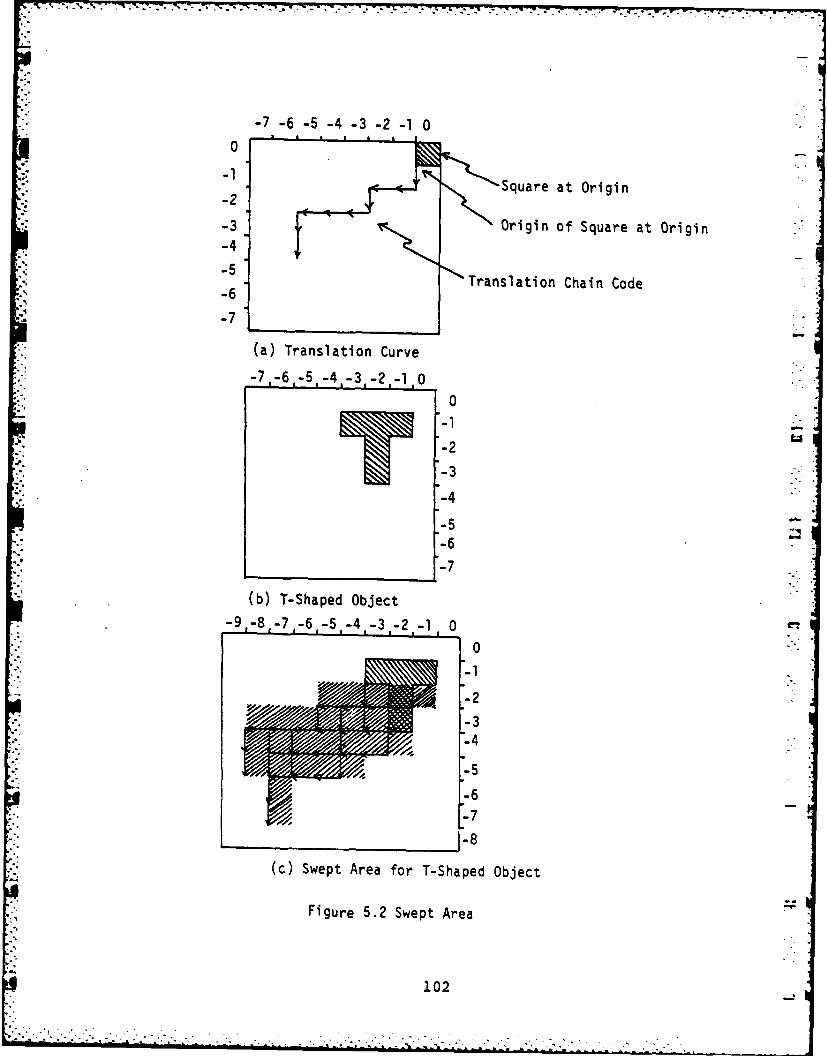
-7 -6 -5 -4 -3 -2 -1 0
0
Square at Origin-2-3 Origin of Square at Origin
-4
-5 Translation Chain Code
-7
(a) Translation Curve
-7,-6,-5,-4,-3,-2,-. 0
0
2
-3-4
-6"-7
(b) T-Shaped Object
-9#-8,-7,-6,-5,-4,-3,-2.-I
0
-2
-3~-4
-5-6
-7
(c) Swept Area for T-Shaped Object
Figure 5.2 Swept Area
102

TN T 7-7
* 0 7
-2 5
44~ 3 4
-5 2 -
h(i,j) -6 1___ ___ ___ __ -7 0
0 2 34 5 6 7(a) Sweep of Solid Square at Origin
Origin (h(ij)) (b) Reversed Direction Sweep ofSolid Square at Origin
h(l-i,2-j),iml to 7,J=2 to 7
7 76 6
*5. 5
4 4 --33A
2. 2
110, 0
0 2 3 45 7
*(Square Being Example: i=5, j=4Evaluated) v(k,m) u~~)AND(u(5,4), h(-4,-2)
(c) Output Square Being Evaluated (d) Location of Weighting PatternWhen Evaluation v(1,2)
Figure 5.3 Weighting Pattern
L 103

5.2.3 Hierarchical Swept Volume
The above demonstrates that a translational swept area
(or volume in 3-D) can be generated using a form of
convolution but the technique cannot be directly applied to -
octree objects. In order to allow this, a Rhierarchical
convolution' summation was developed (see E12] for a similar
technique applied to image processing). The weighting
information is contained in an octree-like tree structure. .
The nodes contain weights for input obels just as the
previous weighting function contained weights to be applied
to locations in the input array.
Assume that an obel in an input octree object is being
compared to an obel in a weighting tree (same level, same
location). The value domain of the input obel contains P as
well as the values empty (E) and solid (F) used above. As
with previous octree algorithms, the general strategy will be
to make a final decision if possible or, if not possible,
defer to lower levels.
An "input/weighting node pair" or simply a 'pair" is a
set of two nodes at a common level, one from the input octree
and one from a weighting tree. The input node represents a
fixed obel in the input object's universe. The weighting
node contains the weighting information to be applied to the
input obel. Pairs defining a specific input/weighting.i 4
evaluation are attached to nodes in the output tree being
104
-
. -generated. An output node may have many attached pairs
awaiting evaluation.
If something solid contained within an input obel (an F
node descendant) "causes" part of the output obel being
evaluated to be solid (results in an F node descendant), it
is said to contribute to the output obel.
The operation of the algorithm can be described in
general terms as follows:
S-For each output obel beginning at the root, maintain a
list of input/weighting node pairs which could possibly
contribute to it (the output obel). Starting at the root
... level, evaluate the pairs, eliminating non-contributing
ones (those which evaluate to a value of E), passing
. appropriately ordered child pairs to the children of the
output obel and their adjacent obel(s) (if not previously
determined to be solid). Operation is terminated at the
* level of the chain code input.
Because of its hierarchical nature, the- weighting tree
cannot contain only binary values. Each node will contain
one of four values with special meaning:
.|
105
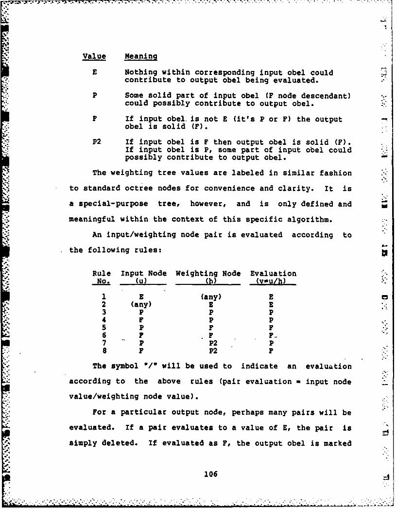
q .....
Value Meaning
E Nothing within corresponding input obel couldcontribute to output obel being evaluated.
P Some solid part of input obel (F node descendant)could possibly contribute to output obel.
F If input obel. is not E (it's P or F) the output -obel is solid (F).
P2 If input obel is F then output obel is solid (F).If input obel is P, some part of input obel couldpossibly contribute to output obel.
The weighting tree values are labeled in similar fashion
to standard octree nodes for convenience and clarity. It is
a special-purpose tree, however, and is only defined and
meaningful within the context of this specific algorithm.
An input/weighting node pair is evaluated according to
the following rules:
Rule Input Node Weighting Node EvaluationNo. (u) (h) (v-u/h)
1 E (any) E 152 (any) E E3 P P P
' 4 F P P5 P F F6 F .FP7 P P2 P8 F P2 F
The symbol ./w will be used to indicate an evaluation
according to the above rules (pair evaluation - input node
value/weighting node value).
For a particular output node, perhaps many pairs will be
evaluated. If a pair evaluates to a value of E, the pair isi simply deleted. If evaluated as F, the output obel is marked
106
6-

*F. If none evaluate to Fe the output is P.' Both F and P
Uevaluated pairs are subdivided into multiple pairs for
distribution to the children (if any) of the output node and
the neighbors of the children (if not already F).
The child pair distribution pattern for a negative going
sweep in 1-D is shown in Figure 5.4. Each node has two
children. Each input/weighting node pair thus has four child
pairs numbered 0 to 3. Two are passed down to child 0 of the
* node. One is passed to child I of the node and one is passed
to child 1 of the neighbor node in the negative direction.
Each child node thus receives about twice as many pairs as
its parent, depending on pair elimination and the pair count
of the parent's neighbor.
S This pattern of child pair transfer is explained by
considering the children of a pair. The two children of the
input node will be u(i) and u(i+l). The two children of the
MW weighting node will be h(k-i) and h(k-(i+l)). There are four
combinations. Of particular interest is the combination of
the earlier input with the later response value (child- pair
1). It cannot contribute -to the output children of the
current output node. It forms one of the terms for the
evaluation of an output node earlier in the sequence of
output nodes (ie.r smaller coordinate value than the output
being evaluated by the original pair in the parent). The
four pairs belong in evaluations as follows:
107
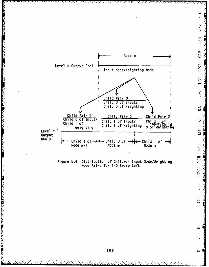
M "-
Node m- iI
I -.
Level Z Output Obel i IInput Node/Weighting Node
Child 0 of Input/iChild 0 of Weighting
I I -'i~I
Child Pair 1 Child Pair 3 Child Pair 2Child 0 of Input/I Child 1 of Input/ Child 1ofI ptChil d 1"f npl/Child 1 of 'Child 1 of Weighting 0 of Cild
weighting gningLevel 2,+1 , tOutput ,Obels J*- Child 1 of-- Child 0 of ->--Child 1 of
Node m-l Node m Node m
Figure 5.4 Distribution of Children Input Node/WeightingNode Pairs for l-D Sweep Left
0.
.. *.. . .--- .. ,-. .- .-.

-- No. Child Pair Output Evaluation Index
0 u(i)/h(k-i) v(k) i1 ui)/h(k- i+l)) v(k-1) i2 u(i+l)/h (k-i) v(k+l) i+13 u(i+l)/h(k-(i+l)) v(k) i+l
Note that output evaluations 0, 2 and 3 are for children
of the original pair.
5.2.4 Weighting Tree Generation
The weighting tree is generated by sweeping test obels
along the sweep curve. The process begins by placing at
location 0,0 in an empty universe a single solid obel at
-. -level n, the level of the chain code represention of the
curve. Conceptually, it is then swept using the standard
U translation and union algorithm along the curve but in the
reverse direction (to account for the negative progression of
the index for the weighting sequence). In practice, more
efficient methods can be used.
A second copy is made of the sweep of the single test
obel. This- is the lowest level of the weighting tree. A
third object is created by sweeping a test obel at level n-i
through the curve beginning, again, at the origin. Its nodesNi "
are then compared to the level n nodes in the original tree
to determine the node values for the level n-i nodes in the
. weighting tree. The following table lists the value
generation rules:
* 109
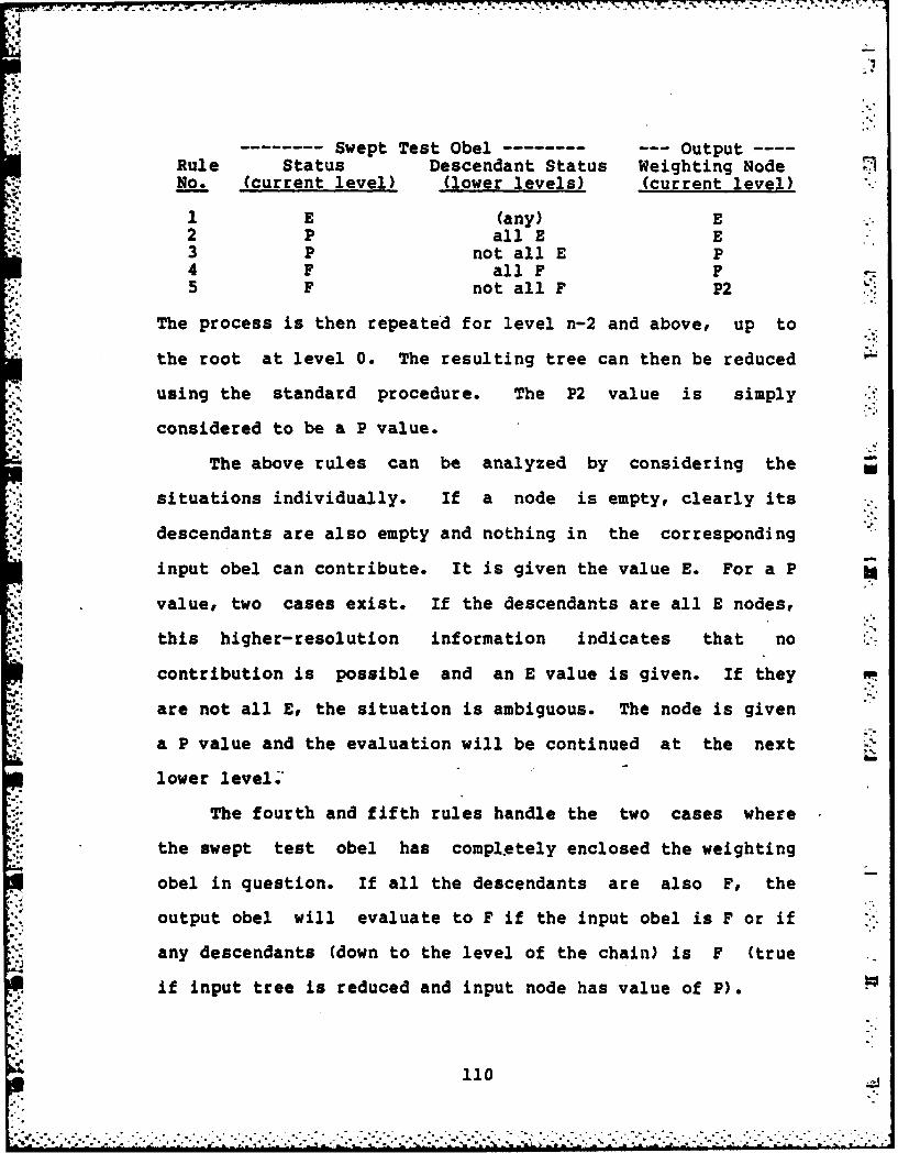
i.?r
Swept Test Obel --- OutputRule Status Descendant Status Weighting NodeNo. (current level) (lower levels) (current level)
1 E (any) E2 P all E E3 P not all E P4 F all F F5 F not all F P2
The process is then repeated for level n-2 and above, up to
the root at level 0. The resulting tree can then be reduced
using the standard procedure. The P2 value is simply
considered to be a P value.
The above rules can be analyzed by considering the
situations individually. If a node is empty, clearly its
descendants are also empty and nothing in the corresponding
input obel can contribute. It is given the value E. For a P
value, two cases exist. If the descendants are all E nodes,
this higher-resolution information indicates that no *. -
contribution is possible and an E value is given. If they
are not all E, the situation is ambiguous. The node is given
a P value and the evaluation will be continued at the next
lower level.*
The fourth and fifth rules handle the two cases where
the swept test obel has compl.etely enclosed the weighting
obel in question. If all the descendants are also F, the
output obel will evaluate to F if the input obel is F or if
any descendants (down to the level of the chain) is F (true
if input tree is reduced and input node has value of P).
110
. . . . . . . I,.* * . *.* * I.- . . . . .o.* '. -- I .. I - - . . . .
If not all the children are P, the information to be
conveyed into the convolution operation is the following. If
1 . the corresponding input obel is solid (F) at this level, then
*+ -. the output obel being evaluated is also solid. If not, the
result is ambiguous. The value P is given to the output and
the final decision is deferred to the lower levels. The
special value for such a weighting node is P2.
-5.2.5 Example of Swept Volume (Hierarchical)
A -D sweep to the left will now be considered as an
example. All objects will be swept left by three steps in a
4-level universe. First the weighting tree is generated.
Figure 5.5(a) shows the result of sweeping a solid obel
located at the origin to the right by 3 steps (reverse of
curve direction) at the four levels. The test obel is solid
and the added swept distance is shaded. At level 3, the
-- , solid obel is swept 3, resulting in the value F for all the
children in the left half of.the universe. At level 2, the
swept distance extends into the right half. At level 1, the
solid object is the left half of the universe. It is stepped
by three level 3 units, covering all but one obel. At level
0, the test obel is the entire universe.
In Figure 5.5(b), the weighting tree is built up. At
-S level 3, it is given the values from the sweep set at level
3. At level 2, the two left obels are marked F based on rule4q
...111
" .. . . .. ... .. ...... "- .I I I A,

Ir
Level0F
F PLevelP -
20 1Level 2 L-F Ej-P E
Level 3 ____ ____ __ ___
(a) Four Sweep Right Level Sets
S.. P2
F EP
P 1 2 30 0
h1(0) F E -h 1(l)-
* (c) Weighting Tree h
Figure 5.5 Weighting Tree Generation
112

4. On the right, obel 2 is set to E based on rule 2 while 3
is set to E from rule 1. At level 1, node 0 becomes F from
rule 4. Node 1 becomes P from rule 3. It is later reduced
to a final value of E. The root is covered by rule 5,
becoming P2.
Figure 5.5(c) is the resulting reduced weighting tree.
Node labeling is as follows. Node f (m) is the node fromn
tree f at level n such that m is the decimal equivalent of
its address string.
An object consisting of segments 4 and 5 as illustrated
in Figure 5.6(a) will be swept. The object could, of course,
be any I-D object, including disjoint sections. The tree for
the object is in Figure 5.6(b).
p Figure 5.7 shows the steps as the algorithm proceeds.
The resulting output object can be expanded to almct:t twite
the size of the input universe. A second (empty) universe is
* added at level 0 on the negative side of the origin forming
"* an augmented universe.
*-. The positive universe at level 0 is- initialized by
attaching the pair containing the roots of the input and
K weighting trees (pair no. 1, P/P2). The pair is evaluated
according to rule 7, resulting in the value P. It is thus
continued into level 1 of the output universe according to
the subdivision rules. The four sets (pairs 2 to 5) are
noted at level 1 in Figure 5.7. All evaluate to E except
pair 4 (u1 (l)/hl(O)). It should be noted that even if all
* 113
5 , .'* "- ---A. -- . ' . • _ .
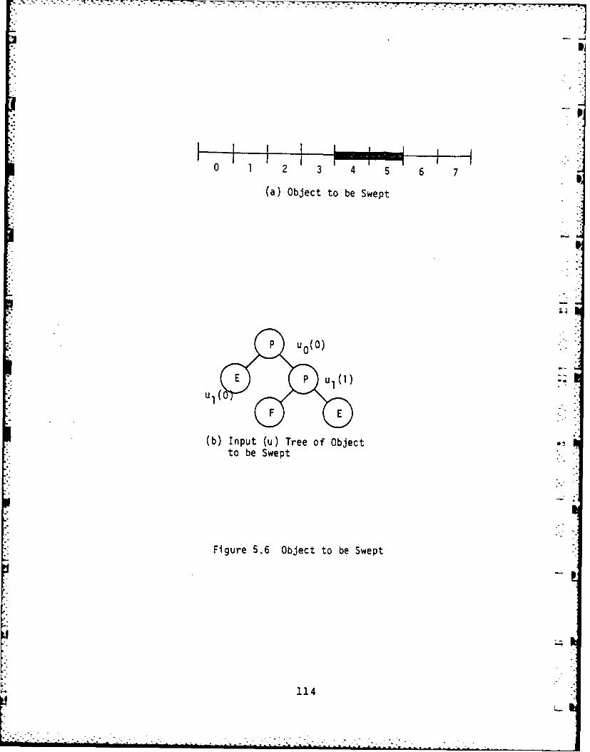
0 4 5 6 7
(a) Object to be Swept
F* E
(b) Input (u) Tree of Objectto be Swept
Figure 5.6 Object to be Swept
114 -

Second (Empty) Universe Added Output UniverseLevel 0
0 0IOrigin
Level 1
,3) u 1 ()/hl(l):2) u 1 (0/h 1(O)=E/F -E 4) u 1l)/h (o)=P/F - P
Level 217) 6)uF (2)/F ()F6)2 :8) u2()p
I F/F -F , F/F- F E/F -Eor
9) u2 (3)/F=
E/F -~E
Level 310)FF-
Output ', 6 AObject
Original Object J444ISwept Left 3 1Level 3 StepsUsing Translation Iand Union 3 Steps Left Local Origin of
Object
Figure 5.7 Example of 1-0 Sweep Algorithm
115
pairs attached to an output node evaluate to E at this level,
that output node will not necessarily be E in the final tree.
An F value may be propagated in from a neighbor at a lower
level. The output node is given a P value and will reduce to
an E later if this fails to occur. A more sophisticated .
algorithm would check neighbor values first. If all are E,
no F could be transferred in. A final value of E could
safely be given.
At level 2, four sets are evaluated (pairs 6 to 9). The
first of the two pairs in the center (pair 6) evaluates to F,
determining a final output value of F for the node. The
second is not considered until child pairs are being
generated.
In a I-D single direction sweep, only one neighbor of
the children need be considered for child pair transfer. In
this case (left sweep) it is the neighbor child to the left.
For pair 7, an F/F evaluation is transfered to the left
neighbor on level 3 (pair 10). Pair 6 has no child pair to
propagate because it has evaluated to F and the neighbor to
the left has already evaluated to F.
The original sweep chain was defined at level 3 and the
process must be terminated here. Operation at lower levels
will cause erroneous results as pairs are carried into
neighbors.
The final output object is the new tree after reduction
as noted in Figure 5.7. It consists of the two F nodes at
116

- ' ..-
level 2 and the single F node at level 3. As a final check,
the original object is swept left using conventional step and
union operations, as shown at the bottom of the figure. The
results are identical.
5.2.6 An yis
For a generalized 1-D sweep in both directions, a
weighting tree extended in the negative direction is
required. The sets of pairs from the negative side would be
generated as above but with a mirrored propagation pattern.
. 2-D four sets of pairs are maintained and in 3-D, 8 sets.
One of the major applications of swept-volume techniques
is in collision avoidance. In such a situation the desired
end result is the spatial intersection of the swept volume
with other objects in the universe. The actual swept-volume
* object is a temporary artifact generated in the process.
Except in extreme situations, the vast bulk of the swept
object is not involved in a collision and is, in a sense,
wasted. If only the sections causing collision were
. calculated, perhaps substantial computational savings would
result.
In the non-hierarchical convolution approach to swept
* - volume represented by (5-4) this can be accomplished by
simply evaluating the convolution only for locations within
L potential collision objects in the universe. There is no
117

need for evaluation to be performed on open space.
In the hierarchical approach, the situation is more
complicated because pairs existing in open space could be
transferred into a collision object at a lower level. It can
be noted, however, that no descendants of a pair will ever
extend beyond the space occupied by the immediate neighbors
of the parent. Thus, for an output node in empty space (in
the collision universe) if all its neighbors are also empty,
all its associated pairs can be deleted. Otherwise, the
child pairs are generated, but only for neighbors which are
not empty (in the collision universe) and have not previously
been determined to be completely occupied.
Most other octree operations involving two or more input
objects, such as set operations, are linear in object
complexity (a constant times the sum of the C valUes places
an upper bound on calculations). They typically perform
comparisons between objects over spatially identical sections
of the universe. Simultaneous traversal over the input trees
visits spatially identical obels because nodes with the same
address represent identical sections of space. A single set
of comparisons for each obel in the output tree is
sufficient.
In the swept volume algorithm, however, the weighting
tree does not represent absolute space. Weighting tree obels
represent space relative to the location of the output obel
being evaluated. Thus, it would be possible for every
118 i

.71
weighting tree node to be examined for each input tree nodei j(no pairs eliminated), in the worst case. Complexity is,
therefore, on the order of the product of the C value for the
input tree and the weighting tree. Because of pair
elimination, much better performance could be expected in
practice than this quadratic upper bound.
The swept-volume algorithm is easily extended for region
growing and region shrinking. The "response" to a solid obel
is an oversized or undersized solid obel. Such operations
are useful for generating fillets, in trajectory planning,
etc. Region shrinking can be used in a breadth-first
traversal to determine the point of closest approach between
two objects. The technique can also be modified slightly to
P perform cross correlation.
The swept volume algorithm can be viewed as an extension
of the overlay concept. Instead of an output obel having a
single overlay which determines its value, a series of
overlays (list of pairs) is employed. The input/weighting
node pairs specify not only the space in the immediate
. vicinity of the output obel but also spatially distant areas.
A second extension has been the use of a special-purpose tree
to specify the decision rules to be employed on a local
basis. Previous algorithms could rely on a single universal
--decision set.
VI
" 119
* .. &.wiiK. ...................... !

. . ..- .. .~ .. .. .' . .
CHAPTER 6
DISPLAY
The display algorithm accepts any number of input
octrees and a set of view parameters (3 view angles,
translation vector and a magnitude factor), and generates a
quadtree containing an orthographic projection image of the
objects, with shaded surfaces and hidden surfaces removed.
Anti-aliasing is an integral part of the algorithm.
A second property, pixel intensity, is added to F (and
possibly P) nodes in the output quadtree. The 2-D object
then becomes a gray-scale image rather than a binary image.
The pre-sorted nature of the octree comes into play when
generating a hidden surface view of one or more octree
objects. By selecting the proper depth-first tree traversal
sequence, the cubes corresponding to the visited nodes are
accessed in a "back-to-front" or "front-to-back" sequence
relative to the viewer.
This is demonstrated in Figure 6.1(a). From the
viewpoint shown, nothing contained in cube 7 can be hidden
from view by an object or part of an object in cubes 0
through 6. In like fashion, nothing in cube 6 can be hidden
by anything in cubes 0 to 5, and so on. If the sequence 7
through 0 is followed recursively, a front-to-back sequence
is generated. As shown in Figure 6.1(b) the first F cube is
120

-- ~~~ 7~' ~ . -
3I
bd (a) Hidden Surface Viewpoint for 7 to 0 Traversal Sequence
p3
123
4* 5
found by repeated selection of the highest numbered child.
Thus, a series of object parts is generated in which A
cubes in the sequence cannot be obscured by cubes later in
the sequence. This eliminates the combinatorial explosion
often encountered in hidden surface removal algorithms. No
terminal node is accessed or examined more than once.
The new display algorithm presented here makes use of a
front-to-back sequence. The visibility of each P node as
well as each F node encountered in the sequence is checked
against the parts of the image previously defined by earlier
F nodes. If completely obscured, the node and all its
children (if P) are discarded. Many hidden sections of the
object or objects are not accessed and do not add to the
computation. Thus the number of calculations required to
generate an image is related to the visual complexity of the
scene rather than the complexity of the objects.P.
Two tree structures are involved. One is a segmentation
of object space (one or more input octrees) and the other, a
segmentation of view space (the output quadtree).
The cubes represented by the nodes of the octree are
projected on the display screen quadtree as shown in Figure
6.2. The projections consist of three 2-D four-sided
polygons as shown in Figure 6.3(a). The bounding box of the
polygon formed by the outer edges is also used as shown in
Figure 6.3(b). In order to avoid confusion in the discussion
to follow, the octree nodes and their projections will be
122

-7 -. 7"T7 ~
Object Node (Octree)
Projection ofObject Node
Display Screen(Quadtree)
-. V Viewer
Figure 6.2 Octree Object Nodes (Cubes) are "Written" IntoDisplay Screen Quadtree
L2 123

7. 7 N. %T...
Projection42 of Node on
# oisplay93 Screen'
Polygon #1
Origin origin Budnof BonfnNode ofn~ Box
Box
(a) Projection of Node on (b) Bounding BoxDisplay Screen
Overlay #2 Overlay '3
Wi ndows
Bounding
Origin ofOverlay
Overlay 00 O0verlay *1
Figure 6.3 Projection of Node (Cube) on Display Screen andOverlay Structure
124

G U
K .:. called simply "nodes." The nodes of the quadtree and the
associated squares on the display screen will be called
"windows."
The basic strategy is to access nodes in the
front-to-back sequence and write them into the quadtree
representing the display screen. Previously undefined
windows enclosed by a node are given a corresponding
intensity value and marked inactive. The quadtree is
-, maintained in a reduced state during algorithm operation.
Each node accessed in the traversal (both branch and
L terminal) is checked for visual intersection with the
quadtree. This can be performed using only simple arithmetic
[431. If it intersects only inactive windows, it is not
I visible and is discarded. The next node in the sequence at
- the same level or higher is then processed. If a branch node
is eliminated in this way, all lower level descendants are
* mautomatically discarded without testing.
The computational load could still be unacceptable if
the number of quadtree windows examined for-each object node
could become arbitrarily large. Once again, overlays will be
used. The intersection test is performed between the node'1.-. .
and exactly four overlay windows. The four windows are the
four possibly intersecting squares at the lowest level such
that the largest dimension of the bounding box of the node is
- the same size or smaller than the edge size of an overlay
square. As shown in Figure 6.3(c), the origin of the
125

bounding box (lower left corner) is always in overlay number
0. It is clear that the four overlay squares will completely
cover the object node.
Thus for each object node in the sequence tested, the
intersection test is performed with four overlays. If all
intersecting overlay windows are inactive, the node and
anything within it are hidden and, therefore, ignored. If
not, additional work is required. For branch nodes, the
eight children are processed in like manner using the four
covering overlay child windows of the parent overlay windows.
For terminal nodes, the children of the overlay windows
- are examined. Any active squares enclosed by the object node
are loaded with the appropriate intensity value and marked
inactive. At the minimum quadtree level, the center of the
window is checked for enclosure. For a detailed description
of the algorithm and the formal procedure, see [411.
For automatic sectioning, a blanking object is traversed
in the same manner as displayed objects. All object nodes
corresponding to an F node in the blanking object are
converted to E nodes and therefore become invisible.
Interference between objects can also be easily detected
during algorithm operation.
The intensity value attached to a quadtree node is the
product of object color (or the texture value for that point
on the object) and the cosine of the angle between the
surface normal and the unit vector to the viewer (the dot
126
product of the two vectors).
For objects defined mathematically, the surface normal
is often easily calculated (or the surface normal times the
" "texture value at that point) and the x, y and z components
are attached to the node. This requires integer
multiplication, may require substantial memory and, in some
,. cases, the local surface normals are not easily computed. In
such cases, block shading is used. The surface intensity
values for the three faces of a cube are calculated.
Quadtree windows enclosed by one of the three faces of a
terminal cube are given the intensity value for that face.
No multiplications are needed. This technique was used for
the images presented in Chapter 7.
_ "Figure 6.4 presents two images of a turbine blade
represented in octree format. In 6.4(a), block shading was
used. In 6.4(b) shading values were generated from unit
.Inormals attached to F nodes on the surface.
The anti-aliasing technique computes intensity values to
. a higher resolution than the screen. The averages of sets of
these values are the pixel intensity values that are then
displayed. The intersection and enclosure tests are
performed to the lower levels. The intensity values for
windows below the screen pixel level are summed into their
,i ancestor windows at the pixel level. At display time, the
". pixel level window values are divided by the appropriate
value (4, 16, ... ) using shifts.
127

- -.
p
7-7.~~~~~. .7 -7 -7 --7. ,
(a) Block Shading
.
(b) Surface - Normal Shading
Figure 6.4 Octree Representation of Turbine Blade
128
.~ . .~

To add multiple illumination sources and shadows, the
display algorithm is performed in reverse. A quadtree loaded
with "illumination" is used. As shown in Figure 6.5, when
nodes are projected on the quadtree they "pick up" and store
whatever illumination is enclosed by the projection. The
corresponding windows are then depleted and cannot illuminate
additional nodes later in the sequence (they are marked
i inactive). This operation is performed once for each source.
If an image is contained in the quadtree, it will be
projected on the object or objects.
After illumination, the display algorithm is performed
to generate an image. The accumulated illumination value for
each node (or each face for block shading) is multiplied by
the surface orientation weight (dot product of normal and
unit vector to viewer) and, possibly, the texture value, to
determine pixel intensity.
1291° "129 *
L_,
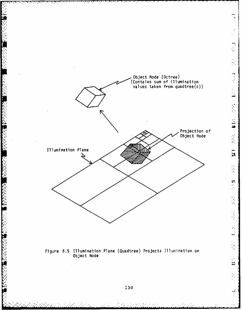
Object Node (Octree)
(Contains sum of illuminationvalues taken from quadtree(s))
Projection of
Object Node
Illumination Plane
Figure 6.5 Illumination Plane (Quadtree) Projects Illumination onObject Node
130
130
!' ., . . . . . .

CHAPTER 7
RESULTS
7.1 Program OCTREE
In order to develop, verify and demonstrate the octree
* .- encoding algorithms, the program OCTREE was written and
implemented on the Prime 750 computer in the Image Processing
Laboratory at RPI. A DeAnza IP5000 color imaging system was
.* used for display.
The program currently encompases 257 routines containing
* 20,696 lines of Fortran code (44,864 if comments are
1P included).
7.1.1 NC Verification
An important function of CAD is the generation of
commands for NC (Numerical Control) machines [83]. A major
problem has been the verification of control programs before
release into production. Traditionally this has been
performed on the machine tool itself and typically requires
the program to be regenerated between three and five times
13114

[26]. The verification task has become a bottleneck and a
major expense in recent years as NC machines have become more
popular, parts have become more complex and labor has become
more expensive. Also, a substantial amount of capital
equipment is removed from production and often tools (and
sometimes the NC machine itself) are damaged.
There has recently been interest in utilizing solid
modeling to replace current methods (84]. Ideally, a parts
programmer or a machinist could verify all phases of an NC
program interactively on a graphics CRT.
In the Fall of 1980, the Center for Manufacturing
Productivity and Technology Transfer (CMP/TT) at RPI funded
an effort through the author to develop a demonstration
system to determine the feasibility of using octree encoding
methods to perform NC verification.
An Imlac 6220 vector graphics terminal with lightpen was
employed to facilitate user interaction. An algorithm was
developed and implemented to extract the forward edges of an
octree object for display.
In operation, the user specifies the workpiece (a block
orthogonal to the axes) using the lightpen. Its octree is
generated and displayed. A specific tool is then requested
and loaded from a disc file. A top view of the workpiece is
then presented. The user selects a starting location and an
endpoint, again using the lightpen. A side view is next
presented for entry of tool depth.
132

At this point the system generates an octree for the
p swept volume of the tool path and subtracts it from the
workpiece. The tool and the workpiece are then displayed.
The user can interactively change the viewpoint or request
the next tool movement.
The program successfully demonstrated the viability of
the technique and has continued to be developed and
embellished by the CMP/TT staff.
* -" Figure 7.1(a) shows a view of a simulated NC milling
* machine. The workpiece contains 40 nodes, the clamp 200
nodes, and the tool 7432 nodes for the bit, 40 nodes for the
S"shaft and 40 nodes for the holder. All 5 objects together
require less than 2000 bytes of storage (serial allocation at
2 bits/node).
. .In Figure 7.1(b) a channel has been machined in the
* ' workpiece. Figures 7.1 (c) through f) show the top, front,
side and orthogonal views after additional material has been
removed.
Using currently available algorithms the program could
be given the capability to detect and display any part of the
original workpiece outside the maximum desired object, any
part of the minimum object removed, and the tolerance object
still remaining after the machining operation.
133
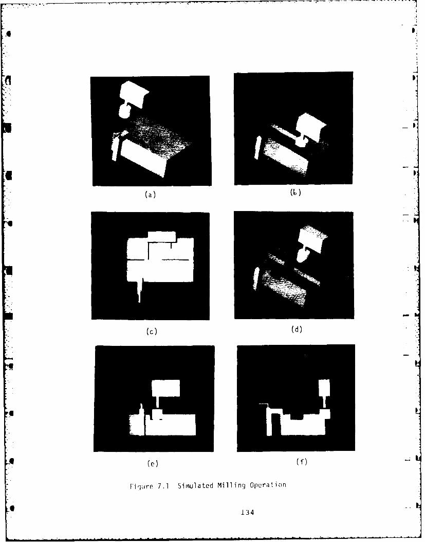
.6f
Figue 7. Simlatd MilingOpertio
(13
LL

:Wi
7.1.2 Medical Imaging
In the spring and summer of 1981, an effort funded by
Phoenix Data Systems, Albany, New York, was undertaken by the
author to investigate the possibility of using octree
encoding methods to interactively generate medical images
derived from CT scans [2, 73, 75-771. Such a capability
would be useful in pre-operative surgical planning [21 and in
other areas. This section reviews the preliminary results.
Ld A series of 42 CT scans of a human head were used for
demonstration and evaluation (scans courtesy Dr. Gabor
Herman, formerly Director of the Medical Image Processing
Group, State University of New York at Buffalo). Thresholded
.-. binary octree objects were generated for display [861.
Figure 7.2 presents 4 views of the section of the skull
p contained in the images. The section extends from just below
to just above eye level. Images 7.2(a) and 7.2(b) are
*. sectioned views of 7.2 (c) and 7.2 (d), respectively.
* . The skull octree in 7.2(c) and 7.2(d) requires 43,112
: ibytes for storage using serial allocation at 2 bits/node
" -*- (C-172,449) whereas the sectioned skull object in 7.2(a)
requires 22,234 bytes 1C-88,937). The original set of imagesS-. (with CT numbers) required over 5.5 million bytes for
* .storage. A more valid compression comparison would be with
the set of thresholded binary images. This would correspond
[13
~135
-9
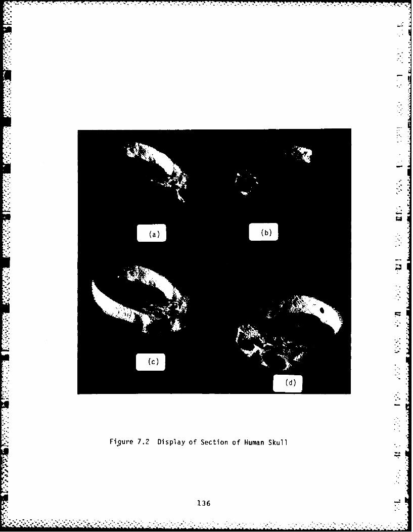
a(a)
'a.'
Figure 7.2 Display of Section of Human Skull
136
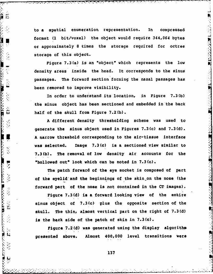
to a spatial enumeration representation. In compressed
format (1 bit/voxel) the object would require 344,064 bytes
or approximately 8 times the storage required for octree
storage of this object.
Figure 7.3(a) is an "object" which represents the low
density areas inside the head. It corresponds to the sinus
passages. The forward section forming the nasal passages has
been removed to improve visibility.
- - In order to understand its location, in Figure 7.3(b)
the sinus object has been sectioned and embedded in the back
u half of the skull from Figure 7.2(b).
A different density thresholding scheme was used to
generate the sinus object used in Figures 7.3(c) and 7.3(d).
U IA narrow threshold corresponding to the air-tissue interface
was selected. Image 7.3(c) is a sectioned view similar to
- 7.3(b). The removal of low density air accounts for the
"hollowed out" look which can be noted in 7.3(c).
The patch forward of the eye socket is composed of part
of the eyelid and the beginnings of the skin on the nose (the
forward part of the nose is not contained in the CT images).
Figure 7.3(d) is a forward looking view of the entire
sinus object of 7.3(c) plus the opposite section of the
skull. The thin, almost vertical part on the right of 7.3(d)
is the back side of the patch of skin in 7.3(c).
L' Figure 7.2(d) was generated using the display algorithm
presented above. Almost 400,000 level transitions were
137
k.
' -°a -°° -°. . '. ° . " ° ° . °% -. • " -. " . -. -." " " " " " .". "..5" "- .'-. ... - " ..

4 1
-7, -

i-i needed, requiring about 11 minutes of CPU time on a Prime
750. Approximately 60% of the octree nodes were accessed.
nAn earlier back-to-front display algorithm (391 was used
to create the remaining images in Figures 7.1 through 7.3.
An algorithm was also developed to display transparent
objects using only simple arithmetic. The resulting images
are very similar to those generated using conventional
transmission x-ray techniques.
L
139
- . . --
CHAPTER 8
DISCUSSION AND CONCLUSIONS
The viability of octree encoding as a solid modeling
method has been demonstrated in two significant examples, NC
verification and medical imaging.
At the current state of development, efficient
algorithms exist to perform the following:
Octree generation from: convex polyhedra, restricted convex
shapes defined mathematically, edges of planar sections (in
chain code format), multiple 2-D images, intersecting prisms,
spatial enumeration arrays, lists of surface intercept points
and swept 2-D or 3-D objects.
Object Property measurement: volume, surface area, center of
mass, moment of inertia, number of interior voids,
correlation, and closest approach between 2 objects.
Obiect operations: union, intersection, difference,
negation, segmentation of disjoint parts,-space filling of
bounded volume, translation, scaling (power of 2 or arbitrary
factor), rotation (multiple of 90 degrees or arbitrary
angle), skewing, reflection, linear and nonlinear
transformations, region growing and shrinking, sectioning,
perspective deformation, and the generation of translational
- or rotational swept volumes.
Interference detection: for fixed or swept objects.
140
. .. .. .-
Display: raster image generation from any viewpoint with
hidden surface removal, orthographic or perspective view,
I black-and-white or color, surface normal or block shading,
shadowing, dynamic movement of light source, multiple
illumination sources, automatic anti-aliasing, sectioning,
interference detection, transparent objects, textured
surfaces, back-to-front or front-to-back traversal, and
raster or quadtree output. Also, vector display of forward
edges of objects (generation and display of edge-tagged
objects).
" 2 The octree method is entirely new and not directly
rooted in any existing system. It is difficult directly to
S"compare this technique with other SMS methods. Rather, a
p iprofile will be obtained by analyzing its characteristics
with respect to the 21 problem areas presented in Section
(1) Limited domain - The domain of objects is completely
unlimited within the restrictions of precision and storage
imposed by a specific implementation. -
(2) Validitv - Any legally generated octree is valid.
(3) ComDleteness - All octrees are complete. No
! .. overhead processing is required to assure this..
(4) Uniqueness - A reduced octree is unique if fixed in
* location and orientation. The octree method thus has
permutational uniqueness but not positional uniqueness.
L (5) Conciseness - In general, conciseness ranges from
141
[ -

- ,.
poor for standard primitive shapes to very favorable for more
arbitrary objects (eg., skulls). One advantage is that, in
its reduced form, there is no redundant information. No
section of space is represented twice.
(6) Closure - The octree encoding method is closed.
(7) Fiiteess - All octree objects are finite.
(8) Null object - The null octree is simply an E root
node (in reduced form).
(9) Transportability- Results should be identical from
one system to another because of the strictly integer
arithmetic. This assumes identical algorithms, scale
factors, etc. It is possible that, unless care is taken,
implementation-specific differences could cause changes in
the conversion of user requests to the integer format
required by the algorithms.
(10) - Extensibility - In general, octree encoding is
easily extended with respect to object size, the number of
objects, object complexity, precision, etc. Assuming that
the dynamic range of integer variables is not exceeded,
standard octree processors should be extensible in these
areas almost without limit.
(11) Autonomy - The algorithms developed to date are
autonomous.
(12) Ri.bilit - All objects which could possibly be
generated can be processed by all compatible algorithms. A
higher level of intelligence is not needed for guidance to
142

handle unusual or special cases.
(13) Efficiency - Within the definition of object
complexity (the value of C), the basic manipulation, analysis
and display algorithms are linear in the number and
complexity of objects. In practice, many algorithms such as
- -display and interference detection, do not require all object
nodes to be processed.
(14) Imnlementability - Octree Encoding algorithms
-" should be easily implemented in multiple VLSI processors
operating in parallel.
(15) Multi~le representations - In operation, two data
structures are envisioned, an application data-base and an
octree structure used for interactive processing.
(16) Consiency- Consistency is not expected to be a
problem because, in most cases, object conversion will be
. -required only from application formats into octrees.
(17) C - Conversion to octree format is a
" straightforward process for most current representation
schemes.
(18) Ease of oblect creation and manipulation - Given
-. high-speed conversion capability and interactive octree
processors, performance in this area should be high when
compared to other methods.
S- (19) Finite-element modeling caDability - The use of
quadtree and octree techniques to automatically generate FEM
L.? meshes was suggested (but not developed) by the author. This
143

area is currently under active investigation at RPI (87].
Preliminary results have been very promising. The automatic 1
placement of smaller squares and cubes in areas of high
curvature has been found to be a useful characteristic.
(20) Interference analysis - Interference detection is
performed in linear time. In many cases it is related to
situation complexity. This is a large improvement over most
competing techniques.
(21) Tweaking - Local modifications can be performed in
isolation because of the spatially sorted nature of the
octree. &
8.1 Accomplishments
A solid modeling method based on a hierarchical tree
structure, the octree, was designed and developed. It is
believed this new method may allow, for the first time, the
construction of relatively inexpensive full-function solid
modeling systems capable of handling large numbers of complex
objects at real-time or near real-time rates. This includes
interference related operations such as interference
detection, collision avoidance and hidden surface removal.
The following are considered to be the most significant
specific results:O
(1) Development of the octree methodology for solid
144
;'vi *. * . .. .**

-. . . o : . . r r . . . . . . . . . ' - . - . - . . . -'
- . ' ' € . ' . ' . " _ -"- . - " -." - ' " - ' -
modeling, with emphasis on performing operations
efficiently using simple integer arithmetic.
(2) An efficient display algorithm based on the use
of front-to-back octree traversal for hidden surface
removal.
(3) A swept-volume generation (and collision
avoidance) algorithm based on hierarchical convolution.
(4) An efficient interference detection algorithm
based on octrees.
8.2 Suggestions for Further Research
The following areas are suggested for further
research:
(1) Alternate object representation format - A
possible research area could be the investigation and
.Nanalysis of alternate formats. For example, obels could
be subdivided into 27 children rather than 8 or':: 2. .. subdivided in only one dimension at each level. This
might lead to more compact representations.
Also, octree methods could probably be used byL •other solid modeling schemes to improve efficiency.
(2) Obiect aeneration - Efficient conversion
- methods are needed for object representations such as
ruled surfaces, surface patches and various parametric
-- formats. Automatic octree generation from wireframe
145

projections [37, 85] could be useful.
(3) Additional operations - Additional analysis and
manipulation techniques would be useful, such as
calculation of curvature and surface normals, volume
conserving deformations, generation of blends and
extrusions, extracting edges for drafting applications,
automatic dimensioning, etc.
(4) Shape classification - It would be desirable to
develop some form of automatic classification of octrees
by shape. Perhaps a start would be to decompose octrees
into primitive shapes or edge/face/vertex sets with
connectivity information.
(5) Advanced finite-element modeling - It may be
possible to utilize octree techniques in finite-element
analysis.
146146
,., ,,,:, :,-,-,, _,-..:,:.;..-,,.:..¢ .- -€:.,:: -,; :..................-......... ..........-.-....... ............-- :...........:...... . ...

CHAPTER 9
REFERENCES
1. Aho, A. V., Hopcroft, J. E. and Ullman, J. D., Theflasign..... and Anal~ysis of Computer Algorit~hms,Addison-Wesley, 1974, 77-78
2. Artzy, £., Frieder, G. and Herman, G. T., "TheTheory, Design, Implementation and Evaluation of aThree-Dimensional Surface Algorithm," Computer Graphicsand Image Processina, Vol. 15, 1981, 1-24
3. Baer, A., Eastman, C., and Henrion, M., "Geometric* Modeling: A Surveyn Com~uter-Aided Design, Vol. 11,
No. 5, Sept. 1979
4. Bentley, J. L.r "Multidimensional Binary Search Treesin Database Applications,* IEEE Transactions onSoft-ware Engineering, Vol. SE-S, No. 4, July 1979
5. Bentley,- J. L. and Wood, D., "An Optimal Worst Case* Algorithm for Reporting Intersections of Rectangles,'
IEEE Transactions on ComRuters, Vol. C-29, No. 7,* July 1980, 571-576
6. Bentley, J.L., 'Multidimensional Divide-and-Conquer,3
Communications of the ACM Vol. 23, No. 4, April 1980
-. 7. Boyse, J. M. and Rosen, J. W., 'GMSOLID - A Systemfor Interactive Design and Analysis of Solids," General
q Motors Research Laboratories publication GMR-3451
8. Boyse, J. W. and Gilchrist, 3. E., 'GMSolid:Interactive Modeling. for Design and Analysis ofSolids,' IEEE Computer graghics and Apolicationst Vol.2, No. 2, March 1982, 27-40
9. Boyse, 3. W., 'Data Structure for a Solid Modeller,'General Motors Research Laboratories publicationBMR-2933, March 1979
10. Brown, C. M.r Requicha, A. A. G. and Voelckerr H.B., 'Geometric Modelling Systems for Mechanical Design
*and Manufacturing,' Production Automation Project,University of Rochester, Oct. 1978
11. Brown, C. M., "PADL-2t A Technical Summary,'"
147

i
Computer Graphics and Aoylications, Vol. 2, No. 2,March 1982, 69-84
12. Burt, P. J., oFast Filter Transforms for Image -Processing," ComDuter Graphics and Image Processnq,No. 16, 1981
13. Bylinsky, G., OA New Industrial Revolution Is on theWay, Fortune, Oct. 5, 1981 _
14. Cadzow, J. A., Discrete-Time Systems, Prentice-Hall,1973, 85-110
15. Catmull, E. and Smith, A. R., "3-D Transformations ofImages in Scanline Order," SIGL2AQ8 1980, 279-285
16. Clark, J., "Hierarchical Geometric Models for VisibleSurface Algorithms," Communications of the ACM, Vol.19, No. 10, Oct. 1976
17. Doctor, L. J. and Torborg, J. G., "DisplayTechniques for Octree-Encoded Objects," IEEE ComputerGraphics and Aplications, Vol. 1, No. 3, July 1981
18. Doctor, L., "Solid Modeling Algorithms Utilizing OctreeEncoding," Center for Interactive Computer Graphics,Rensselaer Polytechnic Institute, December 1980
19. Dyer, C. R., Rosenfeld, A., and Samet, H., "Region
Representation: Boundary Codes from Quadtrees,"Communications of the ACM, Vol. 23, No. 3, larch 1980
20. Finkel, R. A. and Bentley, J. L., "Quad Trees: AData Structure for Retrieval on Composit Keys," ACTAInformtic. Vol. 4, 1974, 1-9
21. Franklin, W. R., "Locating a Point- in OverlappingRegions of Byperspacer Technical Report CLR-64,Rensselaer Polytechnic Institute, Dec. 1978
22. Franklin, W. R., "A Linear Time Exact Hidden SurfaceAlgorithm," Computer Graphics, Vol. 14, No. 3, July ..*
1980
23. Franklin, W. R., "An Exact Hidden Sphere AlgorithmThat Operates in Linear Time," Comouter Graphics andImage Processing, Vol. 15, 1981, 364-379
24. Freeman, H., "Computer Processing of Line-DrawingImages," Computing Surveys, Vol. 6, No. I, March 1974
148
"a,*,. r% .. % % -. ,•Oo . , , .. .. -. .. . -. - . . . . -. -. ,. ., .. -. . ,- - . . •.,- .j .. . %° % - , ' - .. %-.. , - -o"

25. Fuchs, H., "On Visible Surface Generation by A PrioriTree Structures, SIGGRAPH '80, 1980
26. Gossard, D. C. and Tsuchiya, F. S., "NumericalControl Tape Verification Using Graphical Simulation,"CASA Technical Paper, The Computer and AutomatedSystems Association of SME, 1977
27. Grayer, A. R., "Alternative Approaches in GeometricModelling," Computer-Aided Design, Vol. 12, No. 4,July 1980
28. Hillyard, R., "The Build Group of Solid Modelers," IEEEComputer Graphics and ADplications, No. 2, Vol. 2,March 1982, 42-52
29. Hunter, G. M., and Steiglitz, K., "Operations onImages Using Quad Trees," IEEE Transactions on PatternAnalysis and Machine Intelligence, Vol. PAMI-1, No.
"-' 2, April 1979
30. Hunter, G. M., "Efficient Computation and DataStructures for Graphics," PhD dissertation, ElectricalEngineering and Computer Science Department, PrincetonUniversity, June 1978
31. Hunter, G. M., and Steiglitz, K., "LinearTransformation of Pictures Represented by Quad Trees,"
.. Computer Graphics and Image Processing, Vol. 10, July,o,',".--1979
32. Iftikhar, A., "Linear Geometric Transformations onOctrees," M.S. thesis, Electrical, Computer, and
S.. Systems Engineering Department, Rensselaer PolytechnicInstitute, May 1981
33. Jackins, C. L., and Tanimoto, S. L.,_ "Oct-Trees andTheir"Use in Representing Three-Dimensional Objects,"Technical Report 79-07-06, Department of ComputerScience, University of Washington, Seattle, July 1979.
o:.-34. Jacking, C. L., and Tanimoto, S. L., "Oct-Trees and
Their Use in Representing Three-Dimensional Objects,"Computer Graphics and Image Processing, Dec. 1980
35. Jones, L. J., "Solid Modeling: The Future forGraphics," Proceedings of the 1980 CAM-I InternationalSpring Seminar, April 1980
L4
149
.4

36. Khullar, P. and Wang, K. K., "Description and
Interpretation of TIPS-l," Technical Report No. 9, NSF
Injection Molding Project, Cornell University, Oct.1976, revised Aug. 1977
37. Markowsky, G. and Wesley, M. A., "Fleshing Out WireFrames," IBM Journal of Research and Development, Vol.24, No. 5, Sept. 1980, 582-597
38. Meagher, D., "Computer Analysis of Shape: A LiteratureSurvey, IPL-TR-79-001, Image Processing Laboratory,Rensselaer Polytechnic Institute, May 1979
39. Meagher, D., "Octree Encoding: A New Technique for theRepresentation, Manipulation and Display of Arbitrary3-D Objects by Computer," Technical Report-IPL-TR-80-111, Image Processing Laboratory, RensselaerPolytechnic Institute, October 1980
40. Meagher, D., "Geometric Modeling Using OctreeEncoding," Technical Report IPL-TR-81-005, ImageProcessing Laboratory, Rensselaer PolytechnicInstitute, February 1981
41. Meagher, D., "High Speed Display of 3-D Medical ImagesUsing Octree Encoding," IPL-TR-021, Image ProcessingLaboratory, Rensselaer Polytechnic Institute, Sept.1981
42. Meagher, D., "Graphics Package 1 (GP/l) and ProgramOCTREE Programmers Manual," IPL-TR-028, ImageProcessing Laboratory, Rensselaer PolytechnicInstitute, April 1982
43. Meagher, D., "Octree Generation, Analysis andManipulation," IPL-TR-027, Image Processing Laboratory,Rensselaer Polytechnic.Institute, April 1982
44. Meagher, D., "Geometric Modeling Using OctreeEncoding," Computer Graphics and Image Processing, 19,June 1982
45. Meagher, D., "Efficient Synthetic Image Generation ofArbitrary 3-D Objects," Proc. IEEE Computer SocietyConference on Pattern Recognition and Image Processing,June 1982
46. Moravec, H. P., "Three Dimensional Modelling andGraphics with Multiprocessors," internal memo, RoboticsInstitute, Carnegie-Mellon University, Feb. 1980,
150
revised Oct. 1980
47. Myers, Wet "Anf Industrial Perspective on SolidModeling,* IEEE Computer Graphics and Applications,Vol. 2, No. 2, March 1982, 86-97
48. Newman, We M., and Sproull, R. F., Principles ofIntgractive Computer rgraphics, 2nd Ed., McGraw-Hill,1979
49. Okino, N., et al., 'TIPS-i, Technical InformationProcessing Systemr, Institute of Precision Engineering,Hokkaido University, 1978
50. Ranade, S. and Shneier, M., "Using Quadtrees to SmoothImages," IEEE -Transactions on Systems. Man. andCyberne.tics, Vol. SMC-l1, No. 5, May 1981, 373-376
51. Ranade, S., "Use of Quadtrees for Edge Enhancement,3IEEE Transactions on Systems. Man. and Cybernetics,Vol. SMC-l1, No. 5, May 1981, 370-373
* .52. Ranader S., and Shneier, M., "Using Quadtrees to Smooth* .Images," Proceedings of the 5th International
Conference on Pattern Recognition, December 1980
S53. Reddy, D. R. and Rubin, S., *Representation ofThree-Dimensional Objects," CMU-CS-78-113, Dept. ofComputer Science, Carnegie-Mellon University, April1978
54. Requicha, A. A. and Voelckerr H. Be, 'SolidModeling: A Historical Summary and ContemporaryAssessment,6 IEEE Computer GrAphics and Apolications,Vol. 2, No. 2, March 1982, 9-24
55. Requicha, A., and Voelckerr H.,rO 'eometric Modeling ofMechaniical Parts and Machining Processes,* COMPCONTROL
* *- 1979, Sopron, Hungary, Nov. 1979
*56. Requicha, A., "Representations for Rigid Solids:Theory, Methods, and Systems," Comoutinq Surveys, Vol.12, No. 4, December 1980
57. Requicha, A., and Vosicker, Be, 'A TutorialIntroduction to Geometric Modelling,' SIGGRAPH 1980Tutorial, July 1980
58. Rosenfeld, A., "Tree Structures for RegionRepresentation,* Computer Vision Laboratory, University
151 ....

qh -,% ,, . , . .-.
'A
of Maryland, 1979
59. Rosenfeld, A., "Quadtrees and Pyramids for PatternRecognition and Image Processing," Proceedings of the5th International Conference on Pattern Recognition,December 1980
60. Rosenfeld, A. and Kak, A. C., DiQital PictureProcessing, Acaademic Press, 1976, 12-22
61. Roth, S. D., *Ray Casting as a Method for SolidModeling," General Motors Research Laboratorypublication GMR-3466, October 1980
62. Rubin, S. M., and Whitted, T., "A 3-DimensionalRepresentation for Fast Rendering of Complex Scenes,"Computer Graphics, Vol. 14, No. 3, July 1980
63. Samet, H., "A Quadtree Medial Axis Transformation,"TR-803, Computer Science Dept., University of Maryland,August 1979
64. Samet, H., "A Distance Transform for Images Representedby ouadtrees," TR-780, Computer Science Dept.,University of Maryland, 1979
65. Samet, H., "Computing Perimeters of Images Representedby Quadtrees," TR-755, Computer Science Center,University of Maryland, College Park, April 1979
66. Samet, H., "Connected Component Labeling UsingQuadtrees," TR-756, Computer Science Dept., Universityof Maryland, April 1979
67. Samet, H., "Neighbor Finding Techniques for ImagesRepresented by Quadtrees," Computer GraDhics and ImaaeProcgugji , Vol. 18, 1982, 37-57 5
68. Samet, B., "Region Representation: Quadtrees from -
Boundary Codes," Communications of the ACM, Vol. 23,No. 3, March 1980
69. Samet, H., "Region Representation: Raster-to-Quadtree
Conversion," TR-766, Computer Science Dept., Universityof Maryland, May 1979
70. Samet, H., "Region Representation: Quadtree-to-RasterConversion," TR-768, Computer Science Dept., Universityof Maryland, June 1979
152
-'S ,,,".: . ."." "•".". ""." '. "" ." "." " "."". .'.'. ." ".'."". . ,. . -. ': . ...... .','.. .

71. Samet, H., "Region Representation: Quadtree fromBinary Arrays," TR-767, Computer Science Dept.,University of Maryland, May 1979
72. Samet, H., and Rosenfeld, A., "Quadtree Representationof Binary Images," Proceedings of the 5th InternationalConference on Pattern Recognition, December 1980
73. Shani, U., "A 3-D Model-Driven System for theRecognition of Abdominal Anatomy from CT Scans," TR-77,Computer Science Dept., University of Rochester, May1980
74. Shneier, M., "Calculations of Geometric PropertiesUsing Quadtrees" Computer Graphics and Image
. .osis Vol. 16, 1981, 296-302
-4 75. Srihari, S. N., "Representation of Three-DimensionalDigital Images," Technical Report No. 162, Dept. ofComputer Science, State University of New York atBuffalo, July 1980
76. Srihari, S. N., "Hierarchicpl Representations forSerial Section Images," Proceedings of the 5thInternational Conference on Pattern Recognition,December 1980
77. Srihari, S. N., "Representation of Three-DimensionalDigital Images," Computina Surveys, Vol. 13, No. 4,Dec. 1981, 399-424
78. Tanimoto, S. L. OA Pyramid Model for Binary PictureComplexity," Proc. IEEE Computer Society Conference onPattern Recognition and Image Processing, RensselaerPolytechnic Institute, June 1977
.-. 79. Tilove, R. B., *Set. Membership. Classification: AUnified Approach to Geometric Intersection Problems,"IEEE Transactions on CompueAr, Vol. C-29, No. 10,Oct. 1980, 874-883
80. Voelcker, H., and Requicha, A., "Geometric Modeling ofMechanical Parts and Processes," Cmauterl Dec. 1977
81. Voelcker, H., et al., "The PADL-l.0/2 System forDefining and Displaying Solid Objects," ProductionAutomation Project, University of Rochester
82. Wang, X. K. and Ihullar, P., "Computer-Aided Designof Injection Molds Using TIPS-1 System," Cornell
153
iii

K.'
University
83. Welch, A., "Numerical Control Tape Proofing," SME- Technical Paper, Society of Manufacturing Engineers,. 1974
84. Welch, A., "Verification of NC Programs by ComputerSimulation," Manufacturing Engineerina, Sept. 1980,77-82
85. Wesley, M. A., "Construction and Use of GeometricModels," Computer Aided Design Modeling. SystemsEngineering. CAD Systems, edited by J. Encarnacao,Springer Verlag, New York, 1980 -
86. Yau, M. M., and Srihari, S. N., "Recursive Generationof Hierarchical Data Structures for MultidimensionalDigital Images," Technical Report No. 170, Dept. ofComputer Science, State University of New York atBuffalo, January 1981
87. Yerry, M. A. and Shephard, M. S., "Finite ElementMesh Generation Based on a Modified-Quadtree Approach,"Center for Interactive Computer Graphics, RensselaerPolytechnic Institute, March 1982
154
*1
154 T
LJ
' o " .,;*.''..';',, '" . '..,..' ,.''.."" :'-..'" " .,'',..'',,'''.,'L , " " . "" -". " ., , " -". "- . "- , "- ,,".' " ',. , . . '. ',1

UnclassifiedSECURITY CLASSIFICATION OF THIS PAGE ("o DatEute'red)l
REPORT DOCUMENTATION PAGE READ INSTRUCTIONSBEFORE COMPLETING FORM
1. REPORT NUMBER 12.WVT ACCESSIQN No 3. RECIPIENT'S CATALOG NUMBER
.. n I PL-TR-032
4. TITLE (md Subtle. S. TYPE OF REPORT & PERIOD COVERED
The Octree Encoding Method for Efficient TechnicalSolid Modeling
S. PERFORMING ORG. REPORT NUMBER
7. AUTHOR(s) S. CONTRACT OR GRANT NUMBER(a)
Donald J. R. Meagher NOO14-82-K-0301
S. PERFORMING ORGANIZATION NAME AND ADDRESS 10. PROGRAM ELEMENT. PROJECT. TASKAREA & WORK UNIT NUMBERS
Rensselaer Polytechnic InstituteTroy, New York 12181
II. CONTROLLING OFFICE NAME AND ADDRESS 12. REPORT DATE
Office of Naval Research August 1982800 North Qunicy Street 13. NUMBER OF PAGES
Arlington, VA 22217 16414. MONITORING AGENCY NAME & ADDRESS(if dillerent fivo Contollng Office) IS. SECURITY CLASS. (of thle report)
Unclassified
IS&. DECL ASSI FI CATION/DOWN GRADINGSCHEDULE
IS. DISTRIBUTION STATEMENT (of thia Report)
-"The United States Government is authorized to repraduce and distributereprints for governmental purposes notwithstanding any copyright noticeshereon." 1 .. .... ___-
17. DISTRIBUTION STATEMENT (of the abstract entered in Block 20, iI different from Report)
oROVED FOR PUBLIC RELEASE; DISTRIBUTION UNUMITED
IS. SUPPLEMENTARY NOTES
It. KEY WORDS (Contmnue on reeree side if neseea ar Identify by block nmmber)
computer graphicssolid modelingobject manipulation algorithmspattern recognitionoctree representation
* . 20. ABSTRACT (Continue an revrse side It necessary and identify by block number)
Solid modeling is the subject of representing solid objects in a computerto permit their analysis, manipulation and display. This thesis describes thedevelopment of a new solid modeling method called octree encodina, in which ar-
L bitrary objects are represented to a specified resTtioni -ary hierarchicaltrees or "octrees." The number of nodes in an object's octree is used as a
".. easure of object complexity. This number is shown to be on the order of theproduct of object surface area and inverse of the square of the resolution. (over)
DO ,r0A 1473 EDITION OF N OVS61S OBSOLETE Unclassified
SECURITY CLASSIFICATION OF TNIS PACE (I-.en Date - Ntered' .
% ,* ' . * . . ., .

UnclassifiedSECURITY CLASSIFICATION OF THIS PAGE(Whan Data Entered)
|p
A dual data-base approach is proposed. A general-purpose solid-modeling sys-tem based on octree encoding would interactively perform geometric, analyticaland display operations in conjunction with specialized applicatic'I data bases.
Efficient algorithms are presented for the determination of mass properties(volume, surface area, center of mass and moment of inertia, etc.) for the for-mation of new objects via the use of set operations (union, intersection, differ- -ence and negation), for linear transformations (including translation, scalingand rotation), for interference detection, for swept-volume definition,.and fordisplay from any point in space (with surface texture, anti-aliasing and hiddensurface removal). The complexity of the processing required to display anobject is related to the visual complexity of the scene rather than the complex-ity of all objects involved. Interference detection requires computation re-lated to the separation distance between the objects.
The above algorithms require only simple integer arithmetic (addition, sub-traction, magnitude comparison, and shift) in order to facilitate implemention
* in VLSI processors.The new method is compared to existing solid modeling methods in 21 problem
areas.Results are presented which show the application of the technique in the
verification of NC (Numerical Control) machine programming and in the displayof 3-D medical objects derived from multiple CT (Computed Tomography) images.
'*°
Unclassi fled
SECURtITY CLASSIPICA4 .101 OF YU'v PAGEIh~r Data Sneered)
,.,. *,. % *., .... ~ * . * * * * -.

p4
k-'
t4
0P ILE
I Z41,r 4g
~~V4
Airr
'Lit ~ ,.
Id~1 T'c4A.'