行政院國家科學委員會專題研究計畫...
TRANSCRIPT

行政院國家科學委員會專題研究計畫 成果報告
蟻群系統於單機單準則與多準則排程問題之應用(22)
計畫類別個別型計畫
計畫編號 NSC93-2213-E-011-014-
執行期間 93 年 08 月 01 日至 94 年 07 月 31 日
執行單位國立臺灣科技大學工業管理系
計畫主持人廖慶榮
報告類型完整報告
處理方式本計畫涉及專利或其他智慧財產權1年後可公開查詢
中 華 民 國 94 年 10 月 26 日
1
行政院國家科學委員會專題研究計畫成果報告 蟻群系統於單準則與多準則排程問題之應用
Ant Colony Optimization for Scheduling Problems with Single and Multiple Criteria
計畫編號NSC-92-2213- E-011-058 NSC-93-2213-E-011-014 執行期限92 年 8 月 1 日至 94 年 7 月 31 日 主持人廖慶榮 教授 台灣科技大學工業管理系 計畫參與人員曾兆堂 台灣科技大學企業管理系博士班 黃國凌 台灣科技大學工業管理系碩士班 阮曉健 台灣科技大學工業管理系碩士班 廖錚圻 台灣科技大學工業管理系碩士班
中文摘要 本研究中我們設計了不同的三種不同的螞蟻族群最佳化 (Ant Colony OptimizationACO) 演算法來求解單機單目標單機多目標及零工型排程問題本研
究主要區分為以下三部分 Part I ACO 求解考慮相依整備時間的單機環境下之排程問題
在實務界的生產系統中相依整備時間 (sequence-dependent setups) 是排程不可或
缺的考慮因素而其中總延遲時間一直被視為最重要的目標之一但儘管相依整備時間
之延遲問題是如此的重要過去的文獻卻鮮有相關的討論因此在本論文中我們利用
ACO 在單機環境下求解相依整備時間之延遲問題我們提出的螞蟻演算法有一些不同
以往的特色包括導入一個費洛蒙初始值的修正參數以及採用局部搜尋的時機等我們
針對標竿問題來做測試發現它的績效凌駕了許多其它的演算法我們更進一步地將此
演算法應用在無權重的延遲問題上實驗結果顯示此演算法在面對其它擁有最佳表現
的演算法時也能顯現出它的優勢 Part II ACO 求解單機多目標準則之排程問題
我們也嘗試將螞蟻演算法應用在求解最大完工時間以及總延遲時間的單機雙目標
問題上並將它與一種派工法則 ATCS (Apparent Total Cost with Setups) 做比較由實
驗結果得知在此問題下螞蟻演算法亦有相當優秀的表現 Part III 混合以單機為基礎之 ACO 演算法與禁忌演算法來求解典型零工型排程問題
在此部分中我們以瓶頸轉換法的分解概念作為基礎將原本複雜的零工型排程問
題分解為多個單機問題來發展出一種以單機為基礎之 ACO 求解模式並結合禁忌演算
法設計出一種混合型演算法ACO 在許多組合問題上有許多相當不錯的發展在零工
型排程問題的發展上仍屬初步部分原因在於費落蒙收斂性過差有鑑於此我們設計
了一種新型的費落蒙陣列來提升 ACO 在此問題上的搜尋能力輔以禁忌搜尋演算法來
提升求解品質實驗解果顯示此混合演算法在標竿問題的求解中獲得相當良好的效果
而與其他單一或混合演算法相比較仍然具有相當良好的競爭力
2
關鍵詞排程螞蟻演算法相依整備時間總延遲時間雙目標最大完工時間零
工型排程禁忌搜尋 Abstract
In this research we develop three specific ant colony optimization (ACO) algorithms for single machine problem with single criterion and multiple criteria and for job shop scheduling problems The research includes the following three parts
Part I Ant colony optimization for single machine tardiness scheduling with sequence- dependent setups
In many real-world production systems it requires an explicit consideration of sequence-dependent setup times when scheduling jobs As for the scheduling criterion the weighted tardiness is always regarded as one of the most important criteria in practical systems While the importance of the weighted tardiness problem with sequence-dependent setup times has been recognized the problem has received little attention in the scheduling literature In this paper we present an ant colony optimization (ACO) algorithm for such a problem in a single machine environment The proposed ACO algorithm has several features including introducing a new parameter for the initial pheromone trail and adjusting the timing of applying local search among others The proposed algorithm is experimented on the benchmark problem instances and shows its advantage over existing algorithms As a further investigation the algorithm is applied to the unweighted version of the problem Experimental results show that it is very competitive with the existing best-performing algorithms Furthermore we try to apply ACO algorithm to the single machine problem with bi-criteria of makespan and total weighted tardiness The ACO algorithm is compared with the constructive-type heuristic of Apparent Tardiness Cost with Setups (ATCS) and its superiority is demonstrated
Part II Ant colony optimization for single machine scheduling problem with multiple objective scheduling criteria
In this part we try to apply ACO algorithm to the single machine problem with bi-criteria of makespan and total weighted tardiness The ACO algorithm is compared with the constructive-type heuristic of Apparent Tardiness Cost with Setups (ATCS) and its superiority is demonstrated
Part III Ant Colony Optimization combined with Taboo Search for the Job Shop Scheduling Problem
Following the conception of ACO in single machine problems in this part we try to
3
decompose the job shop into several single machine problems and thus a single machine-based ACO combining with taboo search algorithm for the classical job shop scheduling problem is presented ACO has been successfully applied to many combinatorial optimization problems but obtained relatively uncompetitively computational results for this problem To enhance the learning ability of ACO we propose a specific pheromone trails definition inspired from the shifting bottleneck procedure and decompose the job shop scheduling into several single machine problems Furthermore we use a taboo local search to reinforce the schedules generated from the artificial ants The proposed algorithm is experimented on 101 benchmark problem instances and shows its superiority over other novel algorithms In particular our proposed algorithm improves the upper bound on one open benchmark problem instance
Keywords Scheduling Ant colony optimization Weighted tardiness Sequence- dependent setups Taboo search Job shop scheduling Makespan bicriterion
4
Part I Ant colony optimization for single machine tardiness scheduling with sequence-dependent setups 1 Introduction The operations scheduling problems have been studied for over five decades Most of these studies either ignored setup times or assumed them to be independent of job sequence [1] However an explicit consideration of sequence-dependent setup times (SDST) is usually required in many practical industrial situations such as in the printing plastics aluminum textile and chemical industries [2 3] As Wortman [4] indicates the inadequate treatment on SDST will hinder the competitive advantage On the other hand a survey of US manufacturing practices indicates that meeting due dates is the single most important scheduling criterion [5] Among the due-date criteria the weighted tardiness is the most flexible one as it can be used to differentiate between customers
While the importance of the weighted tardiness problem with SDST has been recognized the problem has received little attention in the scheduling literature mainly because of its complexity difficulty This inspires us to develop a heuristic to obtain a near-optimal solution for this practical problem in the single machine environment It is noted that the single machine problem does not necessarily involve only one machine a complicated machine environment with a single bottleneck may be treated as a single machine problem
We now give a formal description of the problem We have n jobs which are all available for processing at time zero on a continuously available single machine The machine can process only one job at a time Associated with each job j is the required
processing time ( jp ) due date ( jd ) and weight ( jw ) In addition there is a setup time ( ijs )
incurred when job j follows job i immediately in the processing sequence Let Q be a sequence of the jobs [ (0) (1) ( )]=Q Q Q Q n where ( )Q k is the index of the thk job in the sequence and (0)Q is a dummy job representing the starting setup of the machine
The completion time of ( )Q k is ( ) ( 1) ( ) ( )1 minus=
= +sum kQ k Q l Q l Q ll
C s p the tardiness of ( )Q k is
( ) ( ) ( )max = minusQ k Q k Q kT C d 0 and the (total) weighted tardiness for sequence Q is
( ) ( )1==sumn
Q Q k Q kkWT w T The objective of the problem is to find a sequence with minimum
weighted tardiness of jobs Using the three-field notation this problem can be denoted by
1 ij j js w Tsum and its unweighted version by 1 sumij js T
Scheduling heuristics can be broadly classified into two categories the constructive type
5
and the improvement type In the literature the best constructive-type heuristic for the
1 ij j js w Tsum problem is Apparent Tardiness Cost with Setups (ATCS) proposed by Lee et
al [8] Like other constructive-type heuristics ATCS can derive a feasible solution quickly but the solution quality is usually unsatisfactory especially for large-sized problems On the other hand the improvement-type heuristic can produce better solutions but with much more
computational efforts For the 1 ij j js w Tsum problem Cicirello [9] develops four different
improvement-type heuristics including LDS (limited discrepancy search) HBSS (heuristic-biased stochastic sampling) VBSS (value-biased stochastic sampling) and VBSS-HC (hill-climbing using VBSS) to obtain solutions for a set of 120 benchmark problem instances each with 60 jobs Recently an SA (simulated annealing) algorithm is used to update 27 such instances in the benchmark library To the best of our knowledge the work of Cicirello [9] is the only research that develops improvement-type heuristics for the
1 ij j js w Tsum problem The importance of the problem in real-world production systems and
its computational complexity deserve us to challenge the problem using a recent metaheuristics the ant colony optimization (ACO) On the other hand there exist several
heuristics of the improvement type for the unweighted problem 1 sumij js T [10 11 12]
2 Literature review 21 Scheduling with sequence-dependent setup times Adding the characteristic of sequence-dependent setup times increases the difficulty of the studied problem This characteristic invalidates the dominance condition as well as the decomposition principle [6]
The importance of explicitly treating sequence-dependent setup times in production scheduling has been emphasized in the scheduling literature In particularly Wilbrecht and Prescott [7] states that this is particularly true where production equipment is being used close to its capacity levels Wortman [4] states that the efficient management of production capacity requires the consideration of setup times
22 1 sumij js T and 1 ij j js w Tsum
Tardiness is a difficult criterion to work with even in the single machine environment There is no simple rule to minimize tardiness with sequence-independent set times except for two special cases (i) the Shortest Processing Time (SPT) scheduling minimizes total tardiness if all jobs are tardy and (ii) the Earliest Due Date (EDD) scheduling minimizes total
6
tardiness if at most one job is tardy [8]Lawler et al [9] show that the 1 j jw Tsum problem is
strongly NP-hard The problem is NP-hard in the ordinary sense when there are no setups and jobs have unit weights [10] Abdul-Razaq et al [11] surveyed algorithms that used both branch and bound as well as DP based algorithms to generate exact solutions ie Solutions are guaranteed to be optimal Potts and Van Wassenhove [12] presented a branch-and-bound algorithm for the single machine total weighted tardiness problem where setup times were assumed to be sequence independent This algorithm can solve up to 40-job problems guarantee the optimality but they require considerable computer resources both in terms of computation times and memory requirements Since the incorporation of setup times
complicates the problem the 1 ij j js w Tsum problem is also strongly NP-hard The
unweighted version 1 sumij js T is strongly NP-hard because max1 ijs C is strongly
NP-hard [13 p 79] and maxC reduces to jTsum in the complexity hierarchy of objective
functions [13 p 27] For such problems there is a need to develop heuristics for obtaining a near-optimal solution within reasonable computation time Two major theoretical developments concern the single machine scheduling tardiness minimization problem Emmons [8] developed the dominance condition and solved two particular cases with constant setups Lawler [9] among others wrote on subject of the decomposition principle These contributions allowed the development of optimal solution procedures but they also inspired the construction of various heuristics
Scheduling heuristics can be broadly classified into two categories the constructive type and the improvement type [14 15] Construction techniques use dispatching rules to build a solution by fixing a job in a position at each step These methods can select jobs for the sequence in a very simple or complex method Simple methods may consist of sorting the jobs by the due date More complex methods may be based on the specific problem structure These methods generally take fewer resources to find a solution but the solution tends to be erratic Both of them are fast and highly efficient but the quality of the solution in not very good The dispatching rule might be a static one ie time dependent like the earliest due date (EDD) rule or a dynamic one ie time dependent like the apparent tardiness cost (ATC) rule Vepsalainen and Morton [15] propose the ATC rule and test efficient dispatching rules for the weighted tardiness problem with specified due date and delay penalties
In the literature the best constructive-type heuristic for the 1 ij j js w Tsum problem is
Apparent Tardiness Cost with Setups (ATCS) proposed by Lee et al [16] This heuristic consists of three phases In the first phase the problem data are used to determine parameters
7
In the second phase the ranking indexes of all unscheduled jobs are computed and the job with the highest priority is sequenced This procedure continues until all jobs are scheduled The third phase of the heuristic consists of a local search performed on a limited neighborhood in which only the most promising moves are considered for evaluation However like other constructive-type heuristics ATCS can derive a feasible solution quickly but the solution quality is usually unsatisfactory especially for large-sized problems On the other hand the improvement-type heuristic can produce better solutions but with much more
computational efforts For the 1 ij j js w Tsum problem Cicirello [17] develops four different
improvement-type heuristics including LDS (limited discrepancy search) HBSS (heuristic-biased stochastic sampling) VBSS (value-biased stochastic sampling) and VBSS-HC (hill-climbing using VBSS) to obtain solutions for a set of 120 benchmark problem instances each with 60 jobs Recently an SA (simulated annealing) algorithm is used to update 27 such instances in the benchmark library To the best of our knowledge the work of Cicirello [17] is the only research that develops improvement-type heuristics for the
1 ij j js w Tsum problem The importance of the problem in real-world production systems and
its computational complexity justify us to challenge the problem using a recent metaheuristic the ant colony optimization (ACO)
On the other hand there exist several heuristics of the improvement type for the
unweighted problem 1 sumij js T among other authors who have treated this problem we
find Ragatz [18] who proposed a branch-and-bound algorithm for the exact solution of smaller instances A genetic algorithm and a local improvement method were proposed by Rubin and Ragatz [6] while Tan and Narasimhan [19] used simulated annealing Finally Gagneacute et al developed the ACO algorithm [26] and the Tabu-VNS algorithm [20] for solving this same problem 23 The ACO algorithm
ACO has been successfully applied to a large number of combinatorial optimization problems including traveling salesman problems [eg 21] vehicle routing problems [eg 22] and quadratic assignment problems [eg 23] which have shown the competitiveness with other metaheuristics ACO has also been used successfully in solving scheduling problems on single machines [eg 24 25 26] and flow shops [eg 27 28] Table 1 lists the available implementations of ACO algorithms
8
3 The background of ACO ACO is inspired by the foraging behavior of real ants which can be described as follows
[33] Real ants have the ability to find the shortest path from a food source to their nest without using visual cue Instead they communicate information about the food source through producing a chemical substance called pheromone laid on their paths Since the shorter paths have a higher traffic density these paths can accumulate higher amount of pheromone Hence the probability of ants following these shorter paths will be higher than the longer ones
ACO is one of the metaheuristics for discrete optimization One of the first applications of the ACO was to the solution of the traveling salesman problem (TSP) [21] A matrix D of the distances ( )d i j between pairs ( i j ) of cities is known and the objective is to find the shortest tour of all cities In the application of the ACO to this problem each ant is seen as an agent with certain characteristics First an ant at city i will choose the next city j to visit taking into account both the distance to each of the existing pheromone on edge ( i j ) Finally the ant k has a memory that prevents returning to those cities already visited This memory is referred to as a tabu list tabuk and is an ordered list of the cities already visited by ant k
We now describe details of the choice process At time t the ant chooses the next city to visit considering a first factor called the trail intensity ( )t i jτ The greater the level of the trail is the greater the probability that will again be chosen by another ant At the initial iteration the trail intensity 0τ is initialized to a small positive quantity The choice of the next city to visit depends also on a second factor called the visibility ( )i jη which is the quantity 1 ( )d i j This visibility acts as a greedy rule that favors the closest cities in the choice process In making the choice of the next city to visit the transition rule ( )p i j allows a trade off between the trail intensity and the visibility (the closest cities) The probability is decided that an ant k will start from city i to city j Parameter β allow control of the trade off between the intensity and the visibility If the total number of ants is m and the number of cities to visit is n a cycle is completed when each ant has completed a tour In the basic version of the ACO the trail intensity is updated at the end of a cycle so as to take into account the evaluation of the tours that have been found in this cycle The evaluation of the tour of ant k is called kL and will influence the trail quantity ( )k i jτΔ that is added to the existing trail on the edges ( i j ) of the chosen tour This quantity is proportional to the length of the tour obtained and is calculated as 1 kL The updating of the trail also takes into account a persistence factor ρ (or evaporation factor 1 ρminus ) This factor serves to diminish the intensity of the existing trail over time Table 1 lists the available implementations of ACO algorithms
9
Table 1 Applications of ACO algorithm to combinatorial optimization problems
Problem type Authors Year Proposed algorithm
Traveling salesman Dorigo Maniezzo and Colorni [34] 1996 AS
Gambardella and Dorigio [35] 1995 Ant-Q
Dorigo and Gambardella [21] 1997 ACS ACS-3-opt
Stutzle and Hoos [36] 1997 MMAS
Bullnheimer Hartl [37] 1999 rankAS
Quadratic assignment Maniezzo Colorni and Dorigo [38] 1994 AS-QAP
Gambardella Taillard and Dorigo [23] 1999 HAS-QAP
Stutzle and Hoos [39] 1998 MMAS-QAP
Maniezzo and Colorni [40] 1999 AS-QAP
Maniezzo [41] 1998 ANTS-QAP
Vehicle routing Bullnheimer Hartl and Strauss [22] 1996 AS-VRP
Gambardella Taillard and Agazzi [42] 1999 HAS-VRP
Scheduling Colorni Dorigo and Maniezzo [43] 1994 AS-JSP
Gagneacute Price and Gravel [26] 2002 ACO
Ying and Liao [27] 2004 ACO-FSP
Trsquokindt Monmarcheacute Tercinet and Lauumlgt [28] 2002 ACO-FSP
Sequential ordering Gambardella and Dorigio [44] 1997 HAS-SOP
10
4 The proposed ACO algorithm The ACO algorithm proposed in this paper is basically the ACS version [21] but it introduces
the feature of minimum pheromone value from ldquomax-min-ant systemrdquo (MMAS) [45] Other elements of MMAS are not applied because there are no significant effects for the studied problem To make the algorithm more efficient and effective we employ two distinctive features along with three other elements used in some ACO algorithms Before elaborating these features we present our ACO algorithm as follows
41 The step of the proposed ACO algorithm
Step 0 Parameter description
Distance adjustment value (β ) In the formulation of ACO algorithm the parameter is used to weigh the relative importance of pheromone trail and of closeness In this way we favor the choice of the next job which is shorter and has a greater amount of pheromone
Transition probability value ( 0q ) 0q is a parameter between 0 and 1 It determines the relative importance of the exploitation of existing information of the sequence and the exploration of new solutions
Decay parameter ( ρ ) In the local updating rule the updating of the trail also takes into account a persistence factor ρ On the contrary 1 ρminus is an evaporation factor The parameter ρ plays the role of a parameter that determines the amount of the reduction the pheromone level
Trail intensity ( ( )t i jτ ) The intensity contains information as to the volume of traffic that previously used edge ( )i j Both the level of the trail and the probability are greater and will again be chosen by another ant At the initial iteration the trail intensity 0 ( )i jτ is initialized to a small positive quantity 0τ
Number of ants ( m ) The parameter m is the total cooperative number of ants
Step 1 Pheromone initialization
Let the initial pheromone trail 0 ATCS( )K n WTτ = sdot where K is a parameter n is the problem size and ATCSWT is the weighted tardiness by applying the dispatching rule of Apparent Tardiness Cost with Setup (ATCS to be elaborated in Step 21)
Step 2 Main loop
In the main loop each of the m ants constructs a sequence of n jobs This loop is executed for Itemax (the maximum of iterations) 1000= iterations or 50 consecutive iterations with no improvement depending on which criterion is satisfied first The latter criterion is used to save computation time for the case of premature convergence
Step 21 Constructing a job sequence by each ant
A set of artificial ants is initially created Each ant starts with an empty sequence and then successively appends an unscheduled job to the partial sequence until a feasible solution is constructed (ie all jobs are scheduled) In choosing the next job j to be appended at the current position i the ant applies the following state transition rule
[ ] [ ] arg max ( ) ( ) if
otherwise
βτ ηisin
⎧ sdot le⎪= ⎨⎪⎩
t 0u Ui u i u q q
jS
11
where ( )t i uτ is the pheromone trail associated with the assignment of job u to position i at time t U is the set of unscheduled jobs q is a random number uniformly distributed in [01] and 0q is a parameter 0(0 1)qle le which determines the relative importance of exploitation versus exploration If 0q qle the unscheduled job j with maximum value is put at position i (exploitation) otherwise a job is chosen according to S (biased exploration) The random variable S is selected according to the probability
[ ] [ ][ ] [ ]( ) ( )
( ) ( ) ( )
t
tu U
i j i jp i j
i u i u
β
β
τ η
τ ηisin
sdot=
sdotsum
The parameter ( )i jη is the heuristic desirability of assigning job j to position i and β is a parameter which determines the relative importance of the heuristic information In our algorithm we use the dispatching rule of Apparent Tardiness Cost with Setups (ATCS) as the heuristic desirability ( )i jη The ATCS rule combines the WSPT (weighted shortest processing time) rule the MS (minimum slack) rule and the SST (shortest setup time) rule each represented by a term in a single ranking index [7] This rule assigns jobs in non-increasing order of ( )jI t v (ie set
( ) ( )ji j I t vη = ) given by
1 2
max( 0)( ) exp exp v jj j j
jj
sw d p tI t v
p k p k sminus minus⎡ ⎤ ⎡ ⎤
= minus minus⎢ ⎥ ⎢ ⎥⎣ ⎦ ⎣ ⎦
where t denotes the current time j j jw p d are the weight processing time and due-date of job j respectively v is the index of the job at position 1i minus p is the average processing time s
is the average setup time 1k is the due date-related parameter and 2k is the setup time-related scaling parameter
Step 22 Local update of pheromone trail
To avoid premature convergence a local trail update is performed The update reduces the pheromone amount for adding a new job so as to discourage the following ants from choosing the same job to put at the same position This is achieved by the following local updating rule
0( ) (1 ) ( )t ti j i jτ ρ τ ρ τ= minus sdot + sdot
where (0 1)ρ ρlt le
Step 23 Local search
The local search in our algorithm is a combination of the interchange (IT) and the insert neighborhood (IS) The IT considers exchanges of jobs placed at the i th and j th positions while the IS inserts the job from the i th position at the j th position We use two of its variants ITIS and ISIT depending on which is implemented first In our algorithm the choice of IT or IS is determined randomly Moreover the local search is applied whenever a better sequence is found during an iteration and it is not executed for those iterations with no improvement The framework of the proposed local search is shown in Figure 2
Step 24 Global update of pheromone trail
The global updating rule is applied after each ant has completed a feasible solution (ie an iteration) Following the rule the pheromone trail is added to the path of the incumbent global best solution ie the best solution found so far If job j is put at position i in the global best solution during iteration t then
12
1( )t i jτ + = (1 ) ( ) ( )t ti j i jα τ α τminus sdot + sdotΔ
where (0 1)α αlt le is a parameter representing the evaporation of pheromone The amount ( ) 1t i j WTτΔ = where WT is the weight tardiness of the global best solution In order to avoid
the solution falling into a local optimum that results from the pheromone evaporating to zero we introduce a lower bound to the pheromone trail value by letting 0( ) (1 5)t i jτ τ=
13
14
42 The distinctive features
The above ACO algorithm has two distinctive features that make it competitive with other algorithms
1 Introducing a new parameter for the initial pheromone trail 2 Adjusting the timing of applying local search
We first discuss the impact of introducing a new parameter for the initial pheromone trail 0τ To incorporate the heuristic information into the initial pheromone trail most ACO algorithms set
0 1( )Hn Lτ = sdot where HL is the objective value of a solution obtained either randomly or through some simple heuristic [13 17 19 20] However our experimental analyses show that this setting of
0τ results in a premature convergence for 1 ij j js w Tsum mainly because the value is too small We thus introduce a new parameter K for 0τ ie 0 ( )HK n Lτ = sdot Detailed experimental results are given in Section 5
As for the second feature we note that in conventional ACO algorithms the local search is executed for the global best solution once within each iteration even for those with no improvement In our algorithm the local search is applied whenever a better solution is found during an iteration Hence the local search may be applied more than once or completely unused in an iteration The computational experiments given in Section 5 show that our approach can save consistently the computation time as many as four times without deteriorating the solution quality The main reason is that the local search in our approach has a higher probability to generate a better solution because the search is performed on a less unexplored space
In addition to the two features there are also some useful elements which have been used in other ACO algorithms being employed in our proposed algorithm These elements include
1 A lower bound for the pheromone trail Stuumltzle and Hoos [45] develop the so-called max-min ant system (MMAS) which introduces upper and lower bounds to the values of pheromone trail Based on our experiments imposing a lower bound to the pheromone trail value improves the solution significantly but there is no significant effect with an upper bound Thus only a lower bound is introduced in our algorithm
2 A local search combining the interchange (IT) and the insert neighborhoods (IS) In our algorithm the local search is a combination of IT and IS [25] We use two of its variants ITIS and ISIT depending on which is implemented first The choice of ITIS or ISIT is determined randomly in our algorithm
3 The job-to-position definition of pheromone trail In general there are two manners to define the pheromone trail in scheduling job-to-job [26] and job-to-position definitions Based on our experimental analyses the job-to-position definition is more efficient than job-to-job for the 1 ij j js w Tsum problem and its unweighted version
5 Computational experiments
To verify the performance of the algorithm two sets of computational experiments were conducted one is for 1 ij j js w Tsum and the other is for its unweighted version 1 ij js Tsum The algorithm was coded in C++ and implemented on a Pentium IV 28 GHz PC 51 1 ij j js w Tsum
In the first set of experiments (for 1 ij j js w Tsum ) the proposed ACO was tested on the 120 benchmark problem instances provided by Cicirello [17] which can be obtained at httpwwwozonericmuedubenchmarksbestknowntxt The problem instances are characterized by three factors (ie due-date tightness δ due-date range R and setup time severity ζ ) and generated by the following parameters 030609δ = 025075R = and 025075ζ =
15
For each combination 10 problem instances each with 60 jobs were generated The best known solutions to these instances were established by applying each of the following improvement-type heuristics LDS (limited discrepancy search) HBSS (heuristic-biased stochastic sampling) VBSS (value-biased stochastic sampling) and VBSS-HC (hill-climbing using VBSS) According to the benchmark library 27 such instances has been updated recently by a simulated annealing algorithm 511 Parameters setting
To determine the best values of parameters a series of pilot experiments was conducted The experimental values of these parameters are as follows α isin 01 03 05 07 09 β isin 05 1 3 5 10 ρ isin 01 03 05 07 09 0q isin 03 05 07 09 095 We show the experimental results in Figure 3~6 The test problem is chosen Cicirellorsquos problem instance 3 where each was run five times The best values for our problem are Itemax 1000= 30=m 001 05 01 09qα β ρ= = = =
2000
2050
2100
2150
2200
2250
2300
2350
wei
ghte
d ta
rdin
ess
Best Average
Best 2125 2129 2196 2201 2199
Average 2204 2245 2238 2327 2305
01 03 05 07 09
Figure 3 The test of parameterα
1900
2000
2100
2200
2300
2400
2500
wei
ghte
d ta
rdin
ess
Best Average
Best 2123 2135 2168 2157 2363
Average 2201 2225 2241 2285 2393
05 1 3 5 10
Figure 4 The test of parameterβ
16
2000
2050
2100
2150
2200
2250
2300
2350
wei
ghte
d ta
rdin
ess
Best Average
Best 2121 2154 2127 2219 2235
Average 2163 2220 2206 2258 2289
01 03 05 07 09
Figure 5 The test of parameter ρ
1800
2000
2200
2400
2600
2800
3000
wei
ghte
d ta
rdin
ess
Best Average
Best 2799 2501 2294 2153 2165
Average 2958 2612 2477 2254 2302
03 05 07 09 095
Figure 6 The test of parameter 0q
We now evaluate the impact of adding a new parameter K for the initial pheromone trail To
make a clear comparison we temporarily remove the local search from the algorithm all the other experiments in this paper were done with local search Table 2 gives the computational results for 10 arbitrarily chosen Cicirellorsquos instances where each was run five times Although there is no single best value of K for all the problem instances good results can be obtained by setting
20K = for the problem It can be observed from Table 2 that adding a new parameter 20K = can significantly improve the solutions The experiments were rerun with local search and the same value ( 20=K ) was found suitable
17
Table 2 The impact of introducing a parameter 20=K for the initial pheromone trail
Average Best Problem
1=K
20=K
to 1=K
1=K
20=K
to 1=K
71 179892 172487 minus41 174341 164671 minus55
72 71694 69761 minus27 69787 69657 minus02
73 47322 45809 minus32 46772 43242 minus75
74 61158 49032 minus198 59211 47809 minus193
75 43518 39251 minus98 43484 37291 minus142
76 97201 72494 minus254 88887 68361 minus231
77 61302 52809 minus139 58902 51940 minus118
78 37598 34675 minus78 37309 30274 minus189
79 146437 134360 minus82 142718 132398 minus72
80 62990 45816 minus273 58601 40266 minus313
512 The test of local search
Another preliminary experiment was conducted to evaluate the timing of applying the local search As noted earlier in conventional ACO algorithms the local search is executed once for every iteration but our algorithm applies the local search whenever a better solution is found Table 3 gives the computational results for 10 arbitrarily chosen Cicirellorsquos instances where each was run five times In the experiment the only termination rule is set by letting Itemax 1000= It is seen from the table that the two approaches result in a similar solution quality but our approach requires only about 25 of the computation time as compared to the conventional approach
Table 3 The effect of timing for applying the local search
Average Best Time (sec) Problem Conv New Conv New Conv New
71 157328 + 160022 150521 + 157382 12025 3099 258 72 58011 57669 + 56364 56273 + 12262 3211 262 73 35989 + 36203 34932 + 35108 12131 3145 259 74 37267 37012 + 34508 + 34964 12152 3180 262 75 34305 32013 + 32990 29878 + 11866 3142 265 76 68225 67936 + 67084 65317 + 12605 3302 262 77 40113 + 40539 37247 + 37896 12189 3314 272 78 28987 25998 + 27308 25213 + 12352 3184 258 79 126553 125293 + 123905 123408 + 12592 3259 259 80 28488 + 29033 27401 + 27796 13030 3430 263
Conv the conventional approach New the new approach used in our algorithm 513 Results and discussions
We now present the formal experimental results for 1 ij j js w Tsum Table 4 shows the comparison between the solutions from our ACO algorithm denoted by ACOLJ thereafter and the best known solutions to the benchmark instances ACOLJ was run 10 times and the best solution was
18
selected For the 104 instances with non-zero weighted tardiness ACOLJ has produced a better solution in 90 such instances (86) For those with zero weighted tardiness ACOLJ also has obtained the optimal solution The average computation time for each run is only 499 seconds with 16 instances taking more than 10 seconds The comparison of computation times cannot be made because they are not provided in the benchmark library
Table 4 Comparison of the solutions from the proposed ACOLJ with the best-known solutions
Problem
Best- known
ACOLJ
Time (sec) Problem
Best- known
ACOLJ
Time (sec)
1 978 894 + 135 31 0 0 0 dagger 2 6489 6307 + 133 32 0 0 0 dagger 3 2348 2003 + 134 33 0 0 0 dagger 4 8311 8003 + 205 34 0 0 0 dagger 5 5606 5215 + 156 35 0 0 0 dagger 6 8244 5788 + 448 36 0 0 0 dagger 7 4347 4150 + 135 37 2407 2078 + 370
8 327 159 + 804 38 0 0 0 dagger 9 7598 7490 + 269 39 0 0 0 dagger
10 2451 2345 + 174 40 0 0 0 dagger 11 5263 5093 + 646 41 73176 73578 ndash 757 12 0 0 1208 42 61859 60914 + 149 13 6147 5962 + 843 43 149990 149670 + 174 14 3941 4035 ndash 709 44 38726 37390 + 133 15 2915 2823 + 2745 45 62760 62535 + 221 16 6711 6153 + 264 46 37992 38779 ndash 167 17 462 443 + 614 47 77189 76011 + 753 18 2514 2059 + 412 48 68920 68852 + 231 19 279 265 + 529 49 84143 81530 + 135 20 4193 4204 ndash 135 50 36235 35507 + 158 21 0 0 0 dagger 51 58574 55794 + 232 22 0 0 0 dagger 52 105367 105203 + 835 23 0 0 0 dagger 53 95452 96218 ndash 644 24 1791 1551 + 0 dagger 54 123558 124132 ndash 363 25 0 0 0 dagger 55 76368 74469 + 271 26 0 0 0 dagger 56 88420 87474 + 180 27 229 137 + 1762 57 70414 67447 + 513 28 72 19 + 1803 58 55522 52752 + 147 29 0 0 0 dagger 59 59060 56902 + 918 30 575 372 + 849 60 73328 72600 + 1254
(Continued on next page)
19
Table 4 (Continued)
Problem
Best- known
ACOLJ
Time(sec)
Problem
Best- known
ACOLJ
Time (sec)
61 79884 80343 ndash 135 91 347175 345421 + 343 62 47860 46466 + 144 92 365779 365217 + 223 63 78822 78081 + 1459 93 410462 412986 ndash 213 64 96378 95113 + 166 94 336299 335550 + 754 65 134881 132078 + 150 95 527909 526916 + 797 66 64054 63278 + 135 96 464403 461484 + 865 67 34899 32315 + 151 97 420287 419370 + 1874 68 26404 26366 + 158 98 532519 533106 ndash 1262 69 75414 64632 + 156 99 374781 370080 + 1788 70 81200 81356 ndash 152 100 441888 441794 + 1236 71 161233 156272 + 150 101 355822 355372 + 137 72 56934 54849 + 135 102 496131 495980 + 1845 73 36465 34082 + 162 103 380170 379913 + 169 74 38292 33725 + 158 104 362008 360756 + 184 75 30980 27248 + 207 105 456364 454890 + 136 76 67553 66847 + 873 106 459925 459615 + 547 77 40558 37257 + 253 107 356645 354097 + 197 78 25105 24795 + 158 108 468111 466063 + 163 79 125824 122051 + 1946 109 415817 414896 + 171 80 31844 26470 + 150 110 421282 421060 + 447 81 387148 387886 ndash 891 111 350723 347233 + 253 82 413488 413181 + 455 112 377418 373238 + 1005 83 466070 464443 + 365 113 263200 262367 + 332 84 331659 330714 + 1781 114 473197 470327 + 519 85 558556 562083 ndash 2078 115 460225 459194 + 2447 86 365783 365199 + 756 116 540231 527459 + 190 87 403016 401535 + 2989 117 518579 512286 + 2182 88 436855 436925 ndash 766 118 357575 352118 + 614 89 416916 412359 + 286 119 583947 584052 ndash 760 90 406939 404105 + 453 120 399700 398590 + 160
+ The proposed algorithm is better ndash The proposed algorithm is worse dagger Computation time less than 01 second for each of 10 runs
20
52 1 ij is Tsum These favorable computational results encourage us to apply our ACOLJ algorithm to the
unweighted problem 1 ij is Tsum Our ACOLJ can be applied to 1 ij is Tsum by simply setting all weights equal to 1 Thus in the second set of the experiments we compare ACOLJ with three best-performing algorithms RSPI ACOGPG and Tabu-VNS for 1 ij is Tsum The RSPI algorithm is a genetic algorithm proposed by Rubin and Ragatz [6] the ACOGPG algorithm is an ACO algorithm developed by Gagneacute et al [26] and the Tabu-VNS algorithm is a hybrid tabu searchvariable neighborhood search algorithm developed by Gagneacute et al [20] Although ACOGPG is also an ACO algorithm it is rather different from our proposed ACOLJ Not only the two features and three elements discussed above are different (eg ACOGPG uses a job-to-job pheromone definition) but ACOGPG has its own feature (eg using look-ahead information in the transition rule) 521 The small and medium-sized problems
To test the small and medium-sized problems (with 15-45 jobs) we use the 32 test problem instances provided by Rubin and Ragatz [6] which can be obtained at httpmgtbusmsuedudatafileshtm Table 5 shows the comparison among RSPI ACOGPG and ACOLJ (the result of Tabu-VNS is not available for the small-sized problems) where ACOGPG gives the best solution from 20 runs and ACOLJ gives the best solution from 10 runs All the three algorithms find the optimal solutions for those 16 instances whose optimal solutions are known For the remaining 16 instances the three algorithms (RSPI ACOGPG and ACOLJ) find the best solutions for 2 (13) 3 (19) and 15 (94) such instances respectively three instances end in a tie
To evaluate the degree of difference in performance we calculate the percentage difference for each of those instances whose solutions are different by ACOGPG and ACOLJ The results are given in the last columns of table 5 A positive value of percentage difference indicates that the ACOGPG is better while a negative value indicates that ACOLJ is better ACOLJ shows an average percentage improvement of 171 for small-sized problems
522 The large-sized problems
To test the large-sized problems (with 55-85 jobs) we use the test problem instances provided by Gagneacute et al [26] and make the comparison among ACOGPG Tabu-VNS and ACOLJ Both ACOGPG and ACOLJ give their best solutions from 20 runs To make our ACOLJ algorithm more efficient and effective some of its parameters were fine tuned 5β = 0 07 5= =q K It can be observed from Table 6 that all the three algorithms find the optimal solutions for those 10 instances whose optimal solutions are known (ie with zero tardiness) For the remaining 22 instances Tabu-VNS is the best for 11 (11 20 55)= instances and ACOLJ is the best for 9 (9 20 45)= instances 2 such cases end in a tie Moreover our ACOLJ has updated 3 instances (Prob551 Prob654 Prob753) with unknown optimal solutions which are provided at httpwwwdimuqacca~c3gagnehome_fichiersProbOrdohtm The comparison of computation times is difficult to make because the computation time of Tabu-VNS is not reported in its paper We simply note that the average computation time of each run for our ACOLJ is 2417 seconds for all the 32 instances
21
Table 5 Comparison of the proposed ACOLJ with two best-performing algorithms for the unweighted
problem (small and medium sized problems)
ACOGPG ACOLJ to Problem RSPI Tsum Time (s) Tsum Time (s) GPG
Prob401 90 90 125 90 0 0
Prob402 0 0 005 0 0 0
Prob403 3418 3418 145 3418 0 0
Prob404 1067 1067 135 1067 0 0
Prob405 0 0 0 0 0 0
Prob406 0 0 0 0 0 0
Prob407 1861 1861 145 1861 0 0
Prob408 5660 5660 145 5660 0 0
Prob501 266 261+ 715 263 105 08 Prob502 0 0 015 0 0 0
Prob503 3497 3497 78 3497 105 0
Prob504 0 0 02 0 0 0
Prob505 0 0 01 0 0 0
Prob506 0 0 01 0 0 0
Prob507 7225 7268 98 7225+ 105 minus06
Prob508 1915 1945 855 1915+ 105 minus15
Prob601 36 16 2975 14+ 115 minus125 Prob602 0 0 04 0 0 0
Prob603 17792 17685 322 17654+ 116 minus02
Prob604 19238 19213 3215 19092+ 116 minus06
Prob605 273 247 3095 240+ 116 minus28
Prob606 0 0 035 0 0 0
Prob607 13048 13088 279 13010+ 117 minus06
Prob608 4733 4733 33 4732+ 116 0
Prob701 118 103 8315 103 237 0 Prob702 0 0 095 0 0 0
Prob703 26745 26663 9175 26568+ 362 minus04
Prob704 15415 15495 8915 15409+ 214 minus06
Prob705 254 222 7755 219+ 337 minus14
Prob706 0 0 09 0 0 0
Prob707 24218 24017 7855 23931+ 461 minus04
Prob708 23158 23351 847 23028+ 136 minus14
indicates optimal solution + The best performance among the three algorithms (ties for all are not indicated)
22
Table 6 Comparison of the proposed ACOLJ with two best-performing algorithms for the unweighted
problem (large-sized problems)
Problem ACOGPG Tabu-VNS ACOLJ
Prob551 212 185 183 + Prob552 0 0 0 Prob553 40828 40644 + 40676 Prob554 15091 14711 14684 + Prob555 0 0 0 Prob556 0 0 0 Prob557 36489 35841 + 36420 Prob558 20624 19872 + 19888
Prob651 295 268 + 268 + Prob652 0 0 0 Prob653 57779 57602 57584 + Prob654 34468 34466 34306 + Prob655 13 2 + 7 Prob656 0 0 0 Prob657 56246 55080 + 55389 Prob658 29308 27187 + 27208
Prob751 263 241 + 241 + Prob752 0 0 0 Prob753 78211 77739 77663 + Prob754 35826 35709 35630 + Prob755 0 0 0 Prob756 0 0 0 Prob757 61513 59763 + 60108 Prob758 40277 38789 38704 +
Prob851 453 384 + 455 Prob852 0 0 0 Prob853 98540 97880 + 98443 Prob854 80693 80122 79553 + Prob855 333 283 + 324 Prob856 0 0 0 Prob857 89654 87244 + 87504 Prob858 77919 75533 75506 +
+ The best performance among the three algorithms (ties for all are not indicated)
23
6 Conclusions In this part we have proposed an ACO algorithm for minimizing the weighted tardiness with
sequence-dependent setup times on a single machine The developed algorithm has two distinctive features including a new parameter for the initial pheromone trail and the change of timing for applying local search These features along with other elements make the algorithm very effective and efficient The algorithm not only updates 86 of the benchmark instances for the weighted tardiness problem but also it is very competitive with the existing best-performing metaheuristics including GA and Tabu-VNS Moreover the algorithm has an excellent performance in computation time
In this research we presents an improvement-type algorithm for the weighted tardiness problem with sequence-dependent setup times on a single machine This problem is important in real-world production system because the tardiness is recognized as the most important criterion and the setup time needs explicit consideration in many situations The importance of the problem in practice deserves the researchers to pay more attention to the problem and its extensions such as in the more complicated job shop environment (see Part III) With the help of recently developed metaheuristics the researchers should be able to tackle more difficult problems in the real world
References [1] Allahverdi A Gupta JND Aldowaisan TA A review of scheduling research involving setup
considerations OMEGA 199927219-39 [2] Das SR Gupta JND Khumawala BM A saving index heuristic algorithm for flowshop
scheduling with sequence dependent set-up times Journal of the Operational Research Society 199546365-73
[3] Gravel M Price WL Gagneacute C Scheduling jobs in an Alcan aluminium factory using a genetic algorithm International Journal of Production Research 2000383031-41
[4] Wortman DB Managing capacity getting the most from your companyrsquos assets Industrial Engineering 19922447-49
[5] Wisner JD Siferd SP A survey of US manufacturing practices in make-to-order machine shops Production and Inventory Management Journal 199511-7
[6] Rubin PA Ragatz GL Scheduling in a sequence dependent setup environment with genetic search Computers and Operations Research 19952285-99
[7] Wilbrecht JK Prescott WB The influence of setup time on job performance Management Science 196916B274-B280
[8] Emmons H One machine sequencing to minimize certain functions of job tardiness Operations Research 196917701-715
[9] Lawler EL A lsquopseudopolynomialrsquo algorithm for sequencing jobs to minimize total tardiness Annals of Discrete Mathematics 19971331-42
[10] Du J Leung JY Minimizing total tardiness on one machine is NP-hard Mathematics of Operations Research 199015483-494
[11] Abdul-Razaq TS Potts CN Van Wassenhove LN A survey of algorithms for the single machine total weighted tardiness scheduling problems Discrete Applied Mathematics 199026235-253
[12] Potts CN Van Wassenhove LN A branch and bound algorithm for the total weighted tardiness problem Operations Research 198533363-377
[13] Pinedo M Scheduling Theory Algorithm and System Englewood Cliffs NJ Prentice-Hall 1995
[14] Potts CN Van Wassenhove LN Single machine tardiness sequencing heuristics IIE Transactions 199123346-354
[15] Vepsalainen APJ Morton TE Priority rules for job shops with weighted tardiness cost Management Science 1987331035-1047
[16] Lee YH Bhaskaram K Pinedo M A heuristic to minimize the total weighted tardiness with
24
sequence-dependent setups IIE Transactions 19972945-52 [17] Cicirello VA Weighted tardiness scheduling with sequence-dependent setups a benchmark
library Technical Report Intelligent Coordination and Logistics Laboratory Robotics Institute Carnegie Mellon University USA 2003
[18] Tan KC Narasimhan R Minimizing tardiness on a single processor with sequence-dependent setup times a simulated annealing approach OMEGA 199725619-34
[19] Gagneacute C Gravel M Price WL A new hybrid Tabu-VNS metaheuristic for solving multiple objective scheduling problems Proceedings of the Fifth Metaheuristics International Conference Kyoto Japan 2003
[20] Dorigo M Gambardella LM Ant colony system a cooperative learning approach to the traveling salesman problem IEEE Transactions on Evolutionary Computation 1997153-66
[21] Bullnheimer B Hartl RF Strauss C An improved ant system algorithm for the vehicle routing problem Annals of Operations Research 199989319-28
[22] Gambardella LM Taillard EacuteD Dorigo M Ant colonies for the quadratic assignment problem Journal of Operational Research Society 199950167-76
[23] Bauer A Bullnheimer B Hartl RF Strauss C An ant colony optimization approach for the single machine total tardiness problem Proceedings of the 1999 Congress on Evolutionary Computation IEEE Press 1999 p 1445-50
[24] Den Besten M Stuumltzle T Dorigo M Ant colony optimization for the total weighted tardiness problem Proceeding PPSN VI 6th International Conference Parallel Problem Solving from Nature vol 1917 Lecture Notes in Computer Science 2000 p 611-20
[25] Gagneacute C Price WL Gravel M Comparing an ACO algorithm with other heuristics for the single machine scheduling problem with sequence-dependent setup times Journal of the Operational Research Society 200253895-906
[26] Ying GC Liao CJ Ant colony system for permutation flow-shop sequencing Computers and Operations Research 200431791-801
[27] Trsquokindt V Monmarcheacute N Tercinet F Lauumlgt D An ant colony optimization algorithm to solve a 2-machine bicriteria flowshop scheduling problem European Journal of Operational Research 200242250-57
[28] Nagar A Haddock J Heragu S Multiple and bicriteria scheduling A literature survey European Journal of Operations Research 19958188-104
[29] Trsquokindt V Billaut JC Some guidelines to solve multicriteria scheduling problems IEEE International Conference on Systems Man and Cybernetics Proceedings 19996463-468
[30] Lee CY Vairaktarakis GL Complexity of single machine hierarchical scheduling A survey Pardalos PM Complexity in Numerical Optimization Singapore World Scientific Publishing Co 1993
[31] Hoogeveen JA Single machine bicriteria scheduling PhD Thesis CWI Amsterdam 1992 [32] Dorigo M Stuumltzle T The ant colony optimization metaheuristics algorithms applications and
advances In Glover F Kochenberger G editors Handbook of metaheuristics vol 57 International Series in Operations Research amp Management Science Kluwer 2002 p 251-85
[33] Dorigo M Maniezzo V Colorni A Ant system Optimization by a colony of cooperating agents IEEE Transactions on System Man and Cybermetics 19962629-41
[34] Gambardella LM Dorigo M Ant-Q A reinforcement learning approach to the traveling salesman problem In Proceedings of the Twelfth International Conference on Machine Learning Palo Alto GA Morgan Kaufmann 1995
[35] Stuumltzle T Hoos HH The MAX-MIN ant system and local search for the traveling salesman problem In Baeck T Michalewicz Z and Yao X editors IEEE International Conference on Evolutionary Computation and Evolutionary Programming Conference 1997
[36] Bullnheimer B Hartl RF Strauss C A new rank-based version of the ant system A computational study Central European Journal for Operations Research and Economics 199923156-174
[37] Maniezzo V Colorni A Dorigo M The ant system applied to the quadratic assignment
25
problem Technical Report IRIDIA 94-128 Belgium 1994 [38] Stuumltzle T Hoos HH The MAX-MIN ant system and local search for combinatorial
optimization problems In Martello SS Osman IH Roucairol C editors Meta-Heuristics Advances and Trends in Local Search Paradigms for Optimization 1998
[39] Maniezzo V Colorni A The ant system applied to the quadratic assignment problem IEEE Transactions on System Knowledge and Date Engineering 199933192-211
[40] Maniezzo V Exact and approximate nondeterministic tree-search procedures for the quadratic assignment problem Technical Report CSR 98-1 Italy 1998
[41] Gambardella LM Taillard EacuteD Agazzi G A multiple ant colony system for vehicle routing problems with time windows In Corne D Dorigo M Glover F editors New Ideas in Optimization United Kingdom McGraw-Hill 199963-76
[42] Colorni A Dorigo M Maniezzo V Trubian M Ant system for job-shop scheduling Belgian Journal of Operations Research 19943439-53
[43] Gambardella LM Dorigo M HAS-SOP An hybrid ant system for the sequential ordering problem Technical Report 11-97 Lugano 1997
[44] Stuumltzle T Hoos HH Max-min ant system Future Generation Computer System 200016889-914
26
Part II Ant colony optimization for single machine scheduling problem with multiple objective scheduling criteria 1 Introduction
The scheduling problem with single criterion has been the subject of considerable research However it has been gradually recognized that practitioners usually consider multiple criteria in scheduling jobs since a single criterion seldom represents the total cost Therefore extensive research on scheduling has been done on the topic of multiple criteria in the past two decades This inspires us to apply ACO algorithm to solve the single machine problem with bi-criteria of makespan and total weighted tardiness The makespan is as important as the total weighed tardiness This is because the makespan represents the degree of the resource utilized by the system Both of the makespan and total weighted tardiness are what the decision maker is concerned about Therefore in this chapter we try to choose makespan and total weighted tardiness as the criteria to be minimized
2 Literature Review Many researchers have been working on multiple criteria scheduling with the majority of work being on bi-criteria scheduling Using two criteria usually makes the problem more realistic than using a single criterion One criterion can be chosen to represent the manufacturerrsquos concern while the other could represent consumerrsquos concern
There are several papers that review the multiple criteria scheduling literature Nagar et al [1] and Trsquokindt and Billaut [2] review the problem in its general form whereas Lee and Vairaktarakis [3] review a special version of the problem where one criterion is set to its best possible value and the other criterion is tried to be optimized under this restriction Also Hoogeveen [4] studies a number of bi-criteria scheduling problems In solving a multiple-criteria scheduling problem there is a difficulty in dealing with several different criteria due to their inconsistency in dimension Fortunately three useful methods have been proposed to solve this difficulty They are the weighting method priority method and efficient solution method The difficulties of applying the first two methods are how actually to find credible weights and satisfactory priorities [5] The efficient solution method resolves the difficulties by generating the complete set of possibly optimal solutions for any objective function involving the chosen criteria Briefly speaking a schedule is efficient if it cannot be dominated by any other schedules It is particularly useful in scheduling because the generated set is relatively small which makes it easier for the decision maker to select the most appropriate solution based on the actual situation To provide the decision maker with more flexibility the efficient solution method is used here to deal with the multiple criteria 3 Apply ACO to max1 ij j js w T Csum In order to increase the efficiency of the ACO algorithm to solve the problem
max1 ij j js w T Csum we change some procedures in our ACO algorithm 1 Update of pheromone trial Now we may have different efficient solutions (non-dominated)
so how we use the local and global update of pheromone trial is a difficulty In our algorithm the choice of which efficient solution used to update is determined by a random manner
2 The timing of applying local search Because of so many efficient solutions if we apply the same timing of applying local search as previous ACO algorithm it will take too much time In order to decrease the time of local search we try to use only two times local search These two times local search are aimed at all efficient solutions we have and one is in a half of maximum iterations and the other is in the end
27
3 ( )t i jτΔ in global update of pheromone trial In single criteria the amount ( ) 1t i j TτΔ = where T is the objective value of the global best solution But now we
have multiple criteria we need a different rule to calculate our objective value We let
1 max 2 j jT w C w W T= + sum where iw is the weight for the associated criterion In the weights of all the criteria are constant the search will always be in the same direction In order to search for various directions we use the variable weights proposed by Murata Ishibuchi Tanaka [6] by assigning a random number iX to each weight iw as follows
1 2
ii
XwX X
=+
4 Computational results
In the remaining of this section we compare the ACO algorithm with constructive-type heuristic of Apparent Tardiness Cost with Setups (ATCS) because ATCS is a dispatching rule which consider makespan and total weighted tardiness these two criteria in single machine with sequence-dependent setup times
In the experiments ACO and ATCS were tested on the problem instance 91~110 provided by Cirirello As for the performance measure the mean relative percentage error (MRPE) is used Let M and WT represent the values of makespan and total weighted tardiness associated with the ACO algorithm and primeM and WT prime the values associated with the ATCS The MRPE of each criterion for the ACO algorithm can be computed as
min( ) 100min( )
M M MM M
primeminustimes
prime
min( ) 100min( )
WT WT WTWT WT
primeminustimes
prime
Similarly the MRPE for ATCS can be computed as min( ) 100
min( )M M M
M Mprime primeminus
timesprime
min( ) 100min( )
WT WT WTWT WT
prime primeminustimes
prime
Because the objective function is to be minimized the smaller the MRPE value the better the algorithm The comparisons of the ACO algorithm with ATCS are summarized in Table 7 Since the ACO algorithm generates a set of efficient schedules each efficient schedule will be compared with the single schedule yielded by ATCS The comparison is done on the average value of the set of efficient schedules From Table 1 it can be seen that the ACO algorithm performs better than ATCS in all two criteria 5 Conclusion
In this part we try to apply ACO algorithm to solve the single machine problem with bi-criteria of makespan and total weighted tardiness In order to fit multiple criteria our ACO algorithm also has three distinctive features including the choice of which efficient solution used to update is determined by a random manner the change of timing for applying local search and a different rule to calculate our objective value for ( )t i jτΔ We compare the ACO algorithm with constructive-type heuristic of Apparent Tardiness Cost with Setups (ATCS) and the ACO algorithm outperforms ATCS in all two criteria of our test problems
In the above two parts we have developed the structural model of applying ACO to different
28
Table 1 Comparison of the ACO algorithm with ATCS
ACO ATCS Problem Makespan Total
weighted tardiness
Makespan Total weighted tardiness
91 0 0 1978 1914 92 0 0 2292 2676 93 0008 0 1506 1831 94 0020 0294 1246 2529 95 0072 0117 1578 2300 96 0 1022 4614 2737 97 0 0161 2914 1782 98 0334 0067 1946 0368 99 0 0126 4255 1904 100 0 0 3179 2544 101 0088 0132 1054 0506 102 0096 0016 0531 0788 103 0 0007 1727 3165 104 0181 0109 1424 0868 105 0103 0059 1113 0491 106 0 0029 1958 1001 107 0136 0214 1108 0439 108 0078 0 0988 1371 109 0077 0476 0863 0690 110 0 0 1610 2938
scheduling problems Since the versatile and robust nature of ACO it shows that the potential and dependable algorithm proposed here is well worth exploring in the context of solving different scheduling problems The proposed ACO heuristic can be extended to deal with other difficult scheduling problems such as multiple identical machines with sequence-dependent setup times or with re-entrant jobs In the chapter on the multiple objective scheduling problems a further improvement is possible Future studies could also extend the ACO algorithm to more complex scheduling environments such as flow-shop job-shop (in ext part) or open shop References [1] Nagar A Haddock J Heragu S Multiple and bicriteria scheduling A literature survey European
Journal of Operations Research 19958188-104 [2] Trsquokindt V Billaut JC Some guidelines to solve multicriteria scheduling problems IEEE
International Conference on Systems Man and Cybernetics Proceedings 19996463-468 [3] Lee CY Vairaktarakis GL Complexity of single machine hierarchical scheduling A survey
Pardalos PM Complexity in Numerical Optimization Singapore World Scientific Publishing Co 1993
[4] Hoogeveen JA Single machine bicriteria scheduling PhD Thesis CWI Amsterdam 1992 [5] Ignizo JP Linear Programming in Single and Multiple Objective Systems NJ Prentice-Hall
1982 [6] Murata T Ishibuchi H Tanaka H Multi-objective genetic algorithm and its applications to
flowshop scheduling Computers and Industrial Engineering 199630957-968
29
Part III Ant Colony Optimization combined with Taboo Search for the Job Shop Scheduling Problem 1 Introduction
The problem that we address in this paper arises in the context of classical job shop scheduling problem (JSSP) In JSSP a set of jobs have to be processed on several machines with the subjection of both conjunctive and disjunctive constraints and the objective of the problem is to minimize the makespan This problem is NP-hard in strong sense [22] not until 1986 could even a relatively small instance with 10 jobs 10 machines and 100 operations be solved optimally
Due to the complexity of JSSP it is unrealistic to solve even a medium-sized problem by using a time-consuming optimization algorithm such as branch and bound schemes or integer programming [9] Therefore metaheuristics such as taboo search [13 27 32] genetic algorithm [11] and simulated annealing [30 35] which are quite good alternatives for JSSP have been studied much in recent years
However each metaheuristic has its own strength and weakness Therefore much research has tried to develop hybrid algorithms expecting to achieve complementarity Those previous experiments have showed that the effectiveness and efficiency of hybrid algorithms are often better than those of single ones [5 17 28 36 37]
In this paper we propose a hybrid algorithm for the problem Following the concept of shifting bottleneck (SB) procedure [1] the proposed algorithm combines ant colony optimization (ACO) with taboo search (TS) to achieve complementarity With the excellent exploration and the information learning ability ACO is expected to provide an appropriate initial schedule This initial schedule can then be locally optimized by TS iteratively
The remainder of this paper is organized as follows In the next section JSSP is formulated mathematically In section 3 the proposed ACO framework is introduced and analyzed Then we describe the local search methods and give the detailed implementation in section 4 Finally computational results for the benchmark problem instances are provided and the proposed algorithm is compared with some best-performing ones
2 Problem definition and notation In JSSP a finite set of jobs is processed on a finite set of machines Each job follows a
predefined machining order and has a deterministic processing time Each machine can process at most one job at a time which cannot be interrupted until its completion A feasible schedule of JSSP is to build a permutation for each machine The objective is to find a feasible schedule that minimizes the makespan
JSSP can be mathematically defined as follows There are a set M of machines a set J of jobs and a set O of operations where ( )j j
m m Oσ σ isin represents a specific operation for job j on machine m Let j
kj
m σσ ≺ be the processing order restriction ie jkσ cannot be processed before the
completion of jmσ Let )(mΠ denote the permutation of jobs on machine ( 1 )m m M= hellip
where ( ) ( 1 )m j j JΠ = hellip is the element of )(mΠ processed in position j Hence a feasible
schedule of JSSP is defined by (1) (2) ( )MΠ = Π Π Πhellip To analyze the problem JSSP can be represented by the disjunctive graph EAVG =
given below [3]
30
sourcesink( ) |
(source ) |
( sink) |
|
j j j j j jm k m k m k
j j j j jk k m m k
j j j j jm m k m ki j i jm m m m
V OA O
O O
O O
E O
σ σ σ σ σ σ
σ σ σ σ σ
σ σ σ σ σ
σ σ σ σ
=
= isin
isin exist isin and
isin exist isin and
= isin
cup≺ cup
≺ cup≺
V is the set of operations where the source and the sink are dummy operations being the representative of the start and end operations of a schedule A is the set of directed arcs connecting consecutive operations of the same job and E is the set of edges that connect operations on the same machine All of the vertices are weighted except for the source and sink A feasible schedule corresponds to orienting disjunctive arcs (edges) to directed ones such that the resulting directed graph is acyclic Given a feasible schedule Π the directed graph ( )G V A E= Π can be created where
cupcup||
1
||
2
))()1(()(M
m
J
j
jmjmE= =
ΠminusΠ=Π
Note that each operation in the disjunctive graph has at most two predecessors and two successors We now introduce the following additional notation to be used in this paper
PT( jmσ ) The processing time of j
mσ MP( j
mσ ) The predecessor of jmσ that processes on machine m
MS( jmσ ) The successor of j
mσ that processes on machine m JP( j
mσ ) The predecessor of jmσ that belongs to the same job j
JS( jmσ ) The successor of j
mσ that belongs to the same job j F( j
mσ ) The longest path from source to jmσ
B( jmσ ) The longest path from j
mσ to sink
)( jmsuc σ The successor sets of j
mσ
)(mπ The processing priority index of machine m
max ( )C Π The makespan value of feasible schedule Π
3 Machine-based Ant Colony Optimization ACO has been successfully applied to a large number of combinatorial optimization problems
including traveling salesman problems [15] vehicle routing problems [8] and quadratic assignment problems [21] all of which show the competitions with other metaheuristics ACO has also been applied successfully to scheduling problems such as single machine problems [6 14 20] and flow shop problems [29 33] However ACO for JSSP generate unsatisfactory results [10 38]
ACO one of the metaheuristics dedicated to discrete optimization problems is inspired by the foraging behavior of real ants which can be stated as follows [16] Real ants are capable of finding the shortest path from a food source to their nest without using any visual cue Instead they communicate information about the food source via depositing a chemical substance called pheromone on the paths The following ants are attracted by the pheromone Since the shorter paths have higher traffic densities these paths can accumulate higher proportion of pheromone Hence the probability of ants following these shorter paths would be higher than that of those following the longer ones
31 The Proposed Algorithm (MACOFT)
We now describe the framework of our proposed hybrid algorithm called machine-based ant
31
colony optimization combined with fast taboo search (MACOFT) Before presenting MACOFT we need to introduce the Shifting Bottleneck (SB) procedure [1] In SB each of the unscheduled machines is considered as a Single Machine Problem (SMP) and the critical machine (the one with the maximum tardiness) is treated as a bottleneck machine that should be scheduled first The SB can be characterized as the following steps subproblem identification bottleneck selection subproblem solution and schedule reoptimization [25] To reduce the computational effort our proposed algorithm constructs schedules on the basis of the similar concept but replaces the essential yet time-consuming step schedule reoptimization with the Proximate Optimality Principle (POP) [3]
The proposed MACOFT can be briefly sketched as follows First we identify the bottleneck machine among all the unscheduled machines Each artificial ant constructs a permutation of the selected machine by using the state transition rule and then deposits an amount of pheromone by applying the local updating rule Periodically the POP is utilized to reoptimize the partial schedule The above steps are repeated until a completely acyclic schedule is established Once all artificial ants have constructed their own schedules the best one is improved by TS Then the pheromone trails are modified again by applying the global updating rule The steps are iterated until a stopping criterion is satisfied Fig 1 outlines the pseudo code of MACOFT where the details of each phase are addressed in what follows while the local search phase is to be elaborated in section 4
Fig 1 The pseudo code of the proposed hybrid algorithm--MACOFT
32 Initialization phase
To reduce the computational effort we identify the bottleneck machine by applying a simple static rule called total machine loading (TML) which can be computed in advance TML is defined
The proposed Hybrid Algorithm--MACOFT
Step 1 Initialization phase Set all the parameters Let all elements in pheromone matrices equal to 0τ Calculate TML ranking indices For Iteration = 1 to MaxIter Do For Ant = 1 to MaxAnt Do
Step2 Construction phase Each artificial ant constructs a permutation of the selected machine by using state transition rule and then deposits amount of pheromone by applying local updating rule Periodically apply POP to reoptimize the partial schedule
End For Step 3 Local search phase Apply fast taboo search to improve the best schedule among all the constructed schedules Step 4 Global updating phase Apply global updating rule to modify the pheromone trails
End for
32
as follows | |
1( ) ( ) 1
Jj
mj
m PT m Mπ σ=
= forall =sum
where )(mπ is the TML ranking index of machine m In this phase a pheromone level 0τ is initialized for all the trails where 0τ is a relatively small quantity
33 Construction phase
331 Definition of pheromone trails for JSSP
Before applying ACO an important issue is to define the pheromone trails [16] For instance the interpretation of pheromone trails in the traveling salesman problem (TSP) refers to the desirability of a path between two connected cities Similarly the ACO for JSSP in the previous research defines pheromone trails as the information level between two operations where the pheromone level is exhibited by a O Otimes pheromone matrix [10]
The construction procedure of traditional ACO for JSSP can be stated as follows [10] All artificial ants are initially placed on the source operation Each artificial ant chooses a next operation to construct a feasible schedule by applying the state transition rule To guarantee the feasibility the selected operation should be chosen from a candidate operation list whose predecessors have been visited Then the selected operation is deleted from the list and its successors are added if they exist The procedure is iterated until the candidate operation list becomes empty In this way a specific feasible topological sequence is generated by each artificial ant
Intuitively this pheromone trails definition may have two problems First permutations of scheduling problems are not the same as those in TSP which are cyclic [15] In other words the relationship between the last and first elements and the first and second elements of a permutation in TSP is the same whereas it is not the same in the scheduling problem Second a feasible schedule (permutation of each machine) of JSSP may have several different topological sequences That is in the traditional approach different topological sequences constructed by different artificial ants may represent the same schedule and thus this might decrease the convergence rate
To overcome the above two shortcomings in MACOFT following SB a M Jtimes JSSP is
decomposed into M separate SMPs That is each artificial ant constructs a permutation for the
selected SMP step by step until all the machines have been scheduled Hence we define M
pheromone matrices with size J Jtimes for their related machines Each of the pheromone matrices is defined by using the absolute position interpretation of pheromone trails which is commonly applied in SMPs and brings better results [6 14]
332 State transition rule
In the construction phase each artificial ant selects an unscheduled machine m with the highest TML level first and chooses the next j
mσ from among a visibility set ( )V V mO O Oisin to guarantee the feasibility by applying the probability state transition rule given below
0max[ ( )] [ ( )] if
otherwise
jm V
jm m
Op j q qβ
στ η σ
σφ
isin⎧ sdot le⎪= ⎨⎪⎩
where ( )m p jτ is the pheromone trail associated with assigning job j to position p with relative pheromone matrix m and ( )j
mη σ is the greedy heuristic desirability of jmσ Parameter
0 0(0 1)q qle le determines the relative proportion between the exploitation and exploration and
(1)
33
parameter β determines the influence of the heuristic information Furthermore φ is a random variable which gives the probability of assigning candidate job i to position p on machine m The value of φ is determined by the probability distribution given below
[ ][ ]( ) ( )
if ( ) ( )Pr( )
0 otherwise
im V
jm m j
m Vijm mm
O
p jO
p i
β
β
σ
τ η σσ
τ η σσisin
⎧ ⎡ ⎤sdot ⎣ ⎦⎪ isin⎪ ⎡ ⎤sdot= ⎨ ⎣ ⎦⎪⎪⎩
sum
The state transition rule resulting from equations (1) and (2) is named as pseudo-random-proportional rule This rule favors the choice of trails with higher pheromone levels When an artificial ant has chosen an operation to move to it samples a random number q If 0qq le then the operation corresponding to the maximum (refer to equation (1)) is chosen (exploitation) else an operation is chosen according to equation (2) (exploration)
333 Delayed precedence constraints
When solving the single machine problem in SB not all the unscheduled operations in the selected machine are executable That is a precedence constraint of two operations may be implied by the sequences of the operations on the machines already scheduled To guarantee the feasibility we implement the delayed precedence constraints (DPCs) described by Dauzere-Peres and Lasserre [12] and Balas et al [4] as follows Each time before solving SMP we use the depth-first search method to obtain the successor set of each candidate operation If there exists an implied precedence constraint on a pair of the unscheduled operations we generate a DPC between the pair
334 Greedy heuristic rule While applying the state transition rule the following two different greedy heuristics are
experimented for the heuristic information )( jmση
(1) Most Work Remaining (MWR) This static heuristic selects the operation belonging to the job with the most remaining processing time
(2) Time Remaining (TR) This dynamic heuristic selects the operation jmσ with the longest
path between jmσ and the dummy sink operation (ie ( ) ( )j j
m mBη σ σ= ) An obvious difference between the static and dynamic greedy heuristics is that the static one
can be computed only once in advance whereas the dynamic one has to be computed in run-time which is time-consuming Moreover to ensure that the constructed schedule is an active schedule we use the insertion technique proposed by Aiex et al [3] Each time when the artificial ant chooses
jmσ we test if the operation can be inserted as early as possible without delaying any other
scheduled operations on machine m
335 Local updating rule
After an artificial ant has completed a permutation of the executed machine m the corresponding pheromone matrix is updated by applying the local updating rule as follows
0( ) (1 ) ( ) ( ) ( )m mp j p j p j mτ ρ τ ρ τ= minus sdot + sdot forall isinΠ
where 0τ is the initial pheromone level and (0 1)ρ ρlt lt is the pheromone evaporating parameter The effect of the local updating rule is to make the choice of putting job j in position p with the related machine less desirable for other artificial ants Consequently artificial ants will favor the exploration of different schedules and prevent putting the same operation in the same position resulting in converging to a common schedule
(2)
34
336 Proximate Optimality Principle
The Proximate Optimality Principle (POP) introduced by Fleurent and Glover [19] is implemented for JSSP by Binato et al [7] In general POP states that good solutions of partial schedules with k operations are close to good solutions of partial schedules with 1k + operations
In MACOFT POP is utilized to reoptimize the partial schedules Our experiments showed that the use of POP could efficiently guide the artificial ants to a good searching space but cost additional computational load Therefore to strike a balance between effectiveness and efficiency empirically POP is not executed after solving every SMP but only executed when a quarter of total operations have been scheduled except for the last quarter (ie 3 times in total) Detailed implementation will be described in section 45
34 Local search phase
In ACO the generated schedules by artificial ants may be so coarse that it should be enhanced by some complementary local search method [25 34] The reason that earlier applications of ACO on JSSP generate unsatisfactory results may be due to the lack of an appropriate local search [16]
To overcome the shortage MACOFT tries to combine ACO with a powerful taboo search method called fast taboo search (FT or TSAB) and proposed by Nowick and Smutnicki [27] Among all the taboo search methods FT can provide relatively competitive effectiveness and efficiency
To generate a good initial schedule for FT is very important but relatively difficult a poor initial schedule cannot guide to a good searching space and cause to inefficiency [25] Thus ACO is expected to provide appropriate initial schedules for FT with its excellent exploration and information learning ability whereas the initial schedules which may be coarse can be refined by FT
To make FT more efficient we further modify its makespan calculation the most time-consuming step Detailed implementation will be given in section 4
35 Global updating phase
This phase is performed after all artificial ants have completed their schedules In order to make the search more directed the global updating rule is intended to provide a greater amount of pheromone to better schedules
Most research in this phase uses the elitist strategy which permits only the global best sequence of the current iteration to deposit pheromone trails [16] However our experimental evidence showed that the elitist strategy might not be suitable for JSSP Statically the elitist strategy may suit for small-sized instances but for relatively large ones (eg 30 jobs 20 machines and 600 operations) updating only the best schedule usually results in poor convergence Therefore there is a need to adjust the parameter of pheromone evaporating rate depending on the instance size As such we propose to update the pheromone trails from a serious of good schedules Once the current best schedule is improved in the local search phase the new best one is stored in a queue called global updating queue An elaboration on this issue will be given in section 43
The definition of the global updating rule is given as follows
( ) (1 ) ( ) ( )m m mp j p j p jτ α τ α τ= minus sdot + sdotΔ
where
max
if ( ) ( ) global updating queue( ) ( )0 otherwise
R
m
OptValue p j mp j Cτ
⎧⎛ ⎞⎪ isinΠ sub⎜ ⎟Δ = Π⎨⎝ ⎠⎪⎩
In the above equation ( )m p jτΔ is the amount of pheromone level added to ( )m p jτ by the
35
artificial ants and parameter α ( 10 lelt α ) is the pheromone evaporation rate which is used to avoid unlimited accumulation of pheromone and enable the algorithm to vanish worse pheromone information OptValue is the optimal value of the makespan (or the best upper bound) and R is set at J in order to discriminate among the schedules in the global updating queue
4 Implementations of local search method In this section we discuss the local search methods employed in MACOFT including FT and
POP
41 Taboo search method
Taboo Search (TS) proposed by Glover is one of the successful local search methods applied in solving combinatorial optimization problems [23 24] The technique can be described as follows TS starts from an initial solution During iterating a move is performed to the best neighboring solution whose quality may not be better than the current one To prevent cycling a short-term memory called taboo list is employed for recording a fixed number of recent moves The use of taboo list avoids returning to a local minimum that has been visited before In addition another memory structure called long-term memory is proposed expecting to expand the searching ability
Many researchers such as Taillard [32] DellrsquoAmico and Trunian [13] and Nowick and Smutnicki [27] apply TS to JSSP and show its superiority Among them the Fast Taboo search (FT or TSAB) proposed by Nowick and Smutnicki [27] is the championship for JSSP Basically FT employs a specific neighborhood definition which effectively reduces the neighborhood size [27]
42 The fast taboo method
FT can be characterized as the following components initial schedule neighborhood definition short-term memory (taboo list) long-term memory stopping criterion Details are described in the following
Consider a given critical path and divide it into several blocks each of which contains at least two operations processed on the same machine We swap the first (last) two successive operations in the last (first) block In others we swap the first and last two successive operations Obviously the neighborhood structure of FT is much smaller than those of other taboo search methods and thus the computational effort can be reduced substantially [32 35]
Once finding a new schedule with a better value during iterating FT stores the triple (schedule neighborhood and taboo list) in the long-term memory When the search is terminated according to the stopping criterion of short-term memory the top element in the long-term memory is retrieved to trace back
In MACOFT the length of taboo list MaxTL is set initially to the magical number 7 [23 24] and changes dynamically depending on the accumulated number of iterations of ACO The value of MaxTL is increased by one after every quarter of the total iterations except for the last quarter is performed (ie MaxTL changes between 7 and 10 inclusively) Let MaxLM be the maximum length of the long-term memory and MaxTabooIter be the stopping criterion of short-term memory Increasing the sizes of MaxLM and MaxTabooIter may yield a higher probability for getting a better schedule but require more computational effort As a tradeoff they are determined experimentally
Furthermore to prevent cycling FT exercises a cyclic test function to judge if there exists a cyclic period (1 Max )δ δ δle le by detecting repetitions of makespan values in time )1(Ο If there exists some period that repeats MaxCycle times then we stop the search and back jump tracking by retrieving the long-term memory list
43 Long-term memory and global updating queue
The proposed global updating queue has a structure similar to the long-term memory While
36
FT is working once a better schedule is found MACOFT immediately updates not only the long-term memory in FT but also the global updating queue Experimentally the length of global updating queue is set at 3 2J M⎢ + ⎥⎣ ⎦ implying that the larger the problem instance sizes are the more schedules the global updating queue has This makes the use of pheromone information more effective
44 The modified makespan calculation
Despite producing high quality results in a reasonable computation time the FT in MACOFT however has to be executed in each iteration causing a heavy computational effort The proposed MACOFT attempts to accelerate the standard FT by using a modified makespan calculation
We begin by analyzing the time complexity of FT In each iteration two dynamic programming formulae are applied to calculate the longest path from operation ( )Oσ σ isin to sink and source as follows
( ) max ( ( )) ( ( )) ( ( )) ( ( )) (3)( ) max ( ( )) ( ( )) ( ) (4)
F F MP PT MP F JP PT JPB B MS B MP PTσ σ σ σ σσ σ σ σ
= + += + +
where (source) (sink) 0F B= = Obviously the makespan can be calculated in time ( )OΟ and
FT can be performed in time ( )h OΟ where h is the size of neighbors
However not all the neighbors need to be calculated by using the standard ( )OΟ makespan calculation Taillard [32] develops a lower bound to reject the worse moves which can be executed in time )1(Ο Supposing that a move )( j
mim σσ is applied the lower bound of the makespan for
the new critical path is calculated by the following equation
max ( ) ( ) ( ) ( )j j i im m m mLB F B F Bσ σ σ σprime prime prime prime= + +
where
( ) max ( ( )) ( ( )) ( ( )) ( ( ))
( ) max ( ) ( ) ( ( )) ( ( ))
( ) max ( ( )) ( ) ( ( )) ( )
( ) max ( ) ( ) ( ( ))
j i i j jm m m m mi j j i im m m m mi j i i im m m m mj i j j
m m m m
F F MP PT MP F JP PT JP
F F PT F JP PT JP
B B MS PT B JS PT
B B PT B JS PT
σ σ σ σ σ
σ σ σ σ σ
σ σ σ σ σ
σ σ σ σ
prime = + +
prime prime= + +
prime = + +
prime prime= + + ( )jmσ
It is easy to see that if LB is greater than the previous makespan then it must be the new value of the critical path on the contrary if we get a less one we should recalculate the makespan value traditionally
However not all the ( ) ( ( ))F Bσ σ of the operations change only those depending upon ( )j i
m mσ σ have to be modified Hence to obtain a new makespan value MACOFT modifies only the set ( ) | ( )j
mF sucσ σ σisin in the new graph by applying (3) which can be performed at most in time ( )OΟ but less in mean case In comparison with the standard FT our experimental results showed that the computational speed was accelerated about 2 times
45 POP with partial disjunctive graph
In MACOFT POP local search is on the basis of FT but works without long-term memory As stated earlier POP is only executed when every quarter of the total operations have been scheduled except for the last quarter The length of POP taboo list (MaxPOPTL) is set at 4 initially and increased by one each time after reaching the stopping criterion (ie MaxPOPTL changes between 4 and 6 inclusively) Another parameter MaxPOPIter which specifies the maximum number of
37
iterations without improving the best partial schedule obtained so far is much less than MaxTabooIter in order to reduce the computational load
Furthermore to accelerate the procedure we substitute the general disjunctive graph by a partial disjunctive graph (PDG) in our POP Let SO denote the set of operations already scheduled where suffix S is the accumulated number of executed machines Then PDG ( )pG V A E= Π is given below
| |
1 2
source sink
( ) |
(source ) |
( sink) |
( ) ( ( ( ) 1) ( ( ) ))
Sj j j j j j
m k m k S m kj j j j j
k k S m S m kj j j j j
m m S k S m kJS
m j
V O
A O
O O
O O
E m j m j
σ σ σ σ σ σ
σ σ σ σ σ
σ σ σ σ σ
π π= =
=
= isin
isin exist isin and
isin exist isin and
Π = Π minus Π
cup cup≺ cup
≺ cup≺
cupcup
Considering only the scheduled operations in PDG implies that we need not only ignore the unscheduled operations along with their adjacent arcs when applying (3) and (4) but also connect the remaining adjacent scheduled operations belonging to the same job with dummy arcs Note that there exist no edges in PDG and the weights of the dummy arcs can be calculated in advance
We now use a numerical example to describe how PDG works Consider a JSSP with 3 machines and 5 jobs as depicted in Fig 2 Given the following partial schedule
)5()4()2( ΠΠΠ=Π where 1 3 22 2 23 2 14 4 43 2 15 5 5
(2)
(4)
(5)
σ σ σ
σ σ σ
σ σ σ
Π =
Π =
Π =
a general disjunctive graph can be illustrated in Fig 3 which has exactly one critical path (source 3
4σ 35σ 2
5σ 15σ 1
4σ 13σ sink) with length 337 Now we apply PDG to modify Fig 3 and illustrate
it in Fig 4 where the unscheduled operations and their adjacent arcs represented by dotted lines are ignored In addition five dummy arcs are added to connect the scheduled operations where their weights are added accordingly When applying the modified makespan calculation the time complexity of PDG is reduced to ( )SOΟ
Note that the notation ( )mjJP σ ( )m
iJS σ and ( )mjPT σ in the proposed modified makespan
calculation should be revised slightly if their adjacent arcs are replaced by the dummy ones For instance since arc 2 1
1 1( )σ σ operation 11 σ and arc 1 5
1 1( )σ σ are ignored the job successor 2 51 1( )JS σ σ= and the processing time )( 2
1σPT depending on its successor may equal either 21 (weight of the original arc) or 74 (weight of the dummy arc) Suppose now that we want to apply the move 3 2
5 5( )σ σ The lower bound can then be calculated as follows 25353525
( ) max039 52 91
( ) max91+16 0+39 107
( ) max84+98 0+183 = 282
( ) max282 160 113 298max107 282 91 298 389
F
F
B
BLB
σ
σ
σ
σ
prime = + =
prime = =
prime =
prime = + + == + + =
where the modified numbers are underlined Since the new lower bound is larger than the previous makespan in Fig 3 (337) the new longest path must pass through 3
5σ and 25σ with makespan
389
38
Fig 2 An example of 5 machines 3 jobs and 15 operations
Fig 3 The general disjunctive graph with three machines being scheduled
Fig 4 The proposed partial disjunctive graph of Fig 3
39
5 Computational results A computational experiment was conducted to evaluate the efficiency and effectiveness of our
proposed MACOFT algorithm which were coded in C++ language and run on a PC with AMD MP-1800+ (1533 MHz) processor
Choosing appropriate parameters is time-consuming and in general depending on the instance such as processing time and instance size Thus we adjust the parameters dynamically when working as follows When MACOFT yields the same makespan value during successive iterations the algorithm is probably falling into a local minimum and hence we raise 0q (utilization of exploration) and α (global pheromone evaporation rate) to give the algorithm a higher probability to escape from the local minimum Table 1 lists all the parameter values used in our experiments
MACOFT was tested on 101 benchmark problem instances of different sizes which can be downloaded from OR-Library web site (httpmscmgamsicacukjeb orlibjobshopinfohtml) The best known lower and upper bounds of Taillardrsquos instances are provided on Taillardrsquos web site (httpinaeivdchcollaborateursetd problemesdirordonnancementdirordonnancementhtml) All the tested problem instances are classified into the following three classes
(a) Nine instances of three different sizes ( J Mtimes = 15 10times 1020times 1515times ) denoted by (LA24 LA25 LA27 LA29 and LA36-LA40) due to Lawrence [26] where problem LA29 is still open
(b) Five instances denoted by (ORB1-ORB5) due to Applegate and Cook [2] two instances (FT10 FT20) due to Fisher and Thompson [18] and five instances (ABZ5-ABZ9) due to Adams et al [1] Problems ABZ8 and ABZ9 are still open
(c) Eighty instances of eight different sizes denoted by (TA01-TA80) due to Taillard [31] These problem instances are solved only for 48 out of 80 instances
Before evaluating the performance of MACOFT we experimented with MACOFT without the local search phase (FT) for both general and partial disjunctive graphs for comparing their computational efficiency All the parameters are set equal including the random seeds to make a fair comparison The experiment was carried out on four different sizes of instances LA36 TA01 TA11 and TA21 each of which was run 5 times Table 2 indicates that using the partial disjunctive graph can accelerate the computational speed about 2 times
Table 1 The setting values of MACOFT parameters
MaxAnt 3M= MaxPOPIter 25= MaxIter 320= MaxPOPTL 4to6=
0 10τ = MaxTabooIter 3000= 1β = MaxLM 3= 01ρ = MaxTL 7 to10=
max 30δ = MaxCycle 6=
0 01 or 035a bq = 085 or 07a bα = a The general parameter set of the algorithm
b The parameter set when falling into local optimum
For the performance measure of the main experiment the relative error RE () was calculated for each instance of problem as a percentage by which the solution obtained (SOL) is above the optimum value (OPT) if it is known or the best lower bound value (LB) [28]
(SOL OPT) 100 (SOL LB) 100RE or REOPT LBminus times minus times
= =
40
Table 2 Computational comparison between partial disjunctive graph (PDG)and general disjunctive graphs (GDG)
Problem J Mtimes (PDG)T ( DG)T G improvement (times)
LA36 15times15 45372 102279 2254 TA01 15times15 44161 96875 2194 TA11 20times15 109914 228194 2095 TA21 20times20 232375 474681 2042
Notes 1 Average computational timeT (in seconds) from 5 runs 2 Improvement ( DG) (PDG)T G T= In the experiments we examined two different heuristic rules on MACOFT MACOFT-MWR
and MACOFT-TR Tables 3 and 4 show the best solutions from 15 runs found for instances (a) and (b) For each algorithm the best value of the makespan (
maxC ) relative error of makespan (RE) and mean relative error (MRE) are listed on the selected problem instances
Table 3 reports the best computational results obtained by Nowicki and Smutnicki [27] (FT) Balas and Vazacopoulos [5] (SB-RGLS2) Pezzella and Merelli [28] (TSSB) and Schultz et al [30] (SHKT-720min) Overall MACOFT-MWR outperforms all the other novel algorithms in terms of solution quality including TSAB (traditional FT method) and TSSB (hybrid algorithm combining TS with SB) Both MACOFT-MWR and MACOFT-TR can be completed in 10 minutes for all of these instances
Table 4 shows the comparison of our algorithms with other novel heuristic algorithms proposed by Aiex et al [3] (GPPR) Schultz et al [30] (SHKT-720min) Pezzella and Merelli [28] (TSSB) on problem instances (b) It is observed from the table that the proposed algorithms produce MREs of 0626 (MACOFT-MWR) and 0689 (MACOFT-TR) both of which exhibit the competition with other novel algorithms
Table 5 lists the computational results for problem instances (c) which contain partially hard instances All the problems were tested for 10 runs where the best makespan (
maxC ) average
makespan ( maxC ) relative error of the best makespan ( maxRE( )C ) and mean relative error (MRE)
are reported Instances (c) include 80 instances where TA51~TA80 are relatively large-sized instances but easy to solve (instances with J much more than M are easy) except for TA62 and TA67 Hence we just list the computational results of TA01-TA50 TA62 and TA67 and omit the easier ones For these instances it is observed that MACOFT-TR performs better than MACOFT-MWR This indicates that the searching ability of MACOFT-TR is superior for large-sized instances Furthermore the columns of maxC show that both proposed algorithms are robust In particular it is noted that MACOFT-TR found a new upper bound 2015 for instance TA41
Table 6 gives the comparison of MACOFT-MWR and MACOFT-TR with other famous hybrid algorithms TSSB and BV-best on instances (c) in terms of MRE average computational time T and numbers of optimal solutions obtained (No OPT) Note that BV-best indicates the best results from all those SB-GLS series provided by Balas and Vazacopoulus [5] Overall MACOFT-TR obtained MRE of 1798 and 40 optimal solutions that are superior to all the others
41
Table 3 Comparison with other algorithms for instances class (a)
TSAB (FT) SB-RGLS2 TSSB SHKT-720min MACOFT-MWR MACOFT-TR Problem OPT or
(LBUB) maxC RE
maxC RE maxC RE
maxC RE maxC RE
maxC RE
LA24 935 939 0428 935 0000 938 0321 938 0321 935 0000 938 0000
LA25 977 977 0000 977 0000 979 0205 977 0000 977 0000 979 0000
LA27 1235 1236 0081 1235 0000 1235 0000 1238 0243 1235 0000 1235 0000
LA29 (11421152) 1160 1576 1164 1926 1168 2277 1161 1664 1158 1401 1163 1839
LA36 1268 1268 0000 1268 0000 1268 0000 1268 0000 1268 0000 1268 0000
LA37 1397 1407 0716 1397 0000 1411 1002 1397 0000 1397 0000 1397 0000
LA38 1196 1196 0000 1196 0000 1201 0418 1196 0000 1196 0000 1196 0000
LA39 1233 1233 0000 1233 0000 1240 0568 1233 0000 1233 0000 1233 0000
LA40 1222 1229 0573 1224 0164 1233 0900 1224 0164 1224 0164 1224 0164
MRE 0375 0232 0632 0266 0174 0223
42
Table 4 Comparison with other algorithms for instances class (b)
GPPR SHKT-720min TSSB MACOFT-MWR MACOFT-TR Problem J Mtimes OPT or
(LBUB) maxC RE
maxC RE maxC RE
maxC RE maxC RE
ORB1 10times10 1059 1059 0000 1059 0000 1064 0472 1059 0000 1064 0000
ORB2 10times10 888 888 0000 888 0000 890 0225 888 0000 890 0000
ORB3 10times10 1005 1005 0000 1005 0000 1013 0796 1005 0000 1013 0000
ORB4 10times10 1005 1005 0000 1005 0000 1013 0796 1005 0000 1013 0000
ORB5 10times10 884 887 0000 887 0000 887 0000 884 0000 887 0000
FT10 10times10 930 930 0000 930 0000 930 0000 930 0000 930 0000
FT20 20times20 1165 1165 0000 1165 0000 1165 0000 1165 0000 1165 0000
ABZ5 10times10 1234 1234 0000 1234 0000 1234 0000 1234 0000 1234 0000
ABZ6 10times10 943 943 0000 943 0000 943 0000 943 0000 943 0000
ABZ7 20times15 656 692 5488 661 0762 666 1524 658 0305 660 0601
ABZ8 20times15 (645665) 705 9302 672 4186 678 5116 670 3876 671 4031
ABZ9 20times15 (661679) 740 1195 687 3933 693 4841 683 3327 685 3631
MRE 2228 0740 1148 0626 0689
43
Table 5 Results by MACOFT for instances class (c) MACOFT-MWR MACOFT-TR
Problem OPT or (LBUB)
maxC maxC maxRE( )C
maxC maxC maxRE( )C
TA01 1231 1231 12321 0000 1231 12334 0000 TA02 1244 1244 12440 0000 1244 12446 0000 TA03 1218 1220 12213 0164 1220 12233 0164 TA04 1175 1175 11803 0000 1175 11801 0000 TA05 1224 1229 12375 0408 1228 12369 0327 TA06 1238 1240 12447 0162 1238 12426 0000 TA07 1227 1228 12312 0081 1228 12320 0081 TA08 1217 1217 12211 0000 1217 12202 0000 TA09 1274 1274 12813 0000 1274 12795 0000 TA10 1241 1241 12483 0000 1241 12462 0000 TA11 (13231361) 1367 13719 3326 1365 13745 3175 TA12 (13511367) 1374 13804 1702 1374 13872 1702 TA13 (12821342) 1349 13611 5226 1350 13592 5304 TA14 1345 1345 13450 0000 1345 13450 0000 TA15 (13041340) 1342 13591 2914 1350 13626 3528 TA16 1302 1362 13747 4608 1362 13701 4608 TA17 1462 1473 14825 0752 1470 14894 0547 TA18 (13691396) 1403 14150 2484 1404 14172 2557 TA19 (12971335) 1341 13526 3392 1341 13555 3392 TA20 (13181351) 1352 13574 258 1353 13591 2656 TA21 (15391644) 1650 16615 7212 1647 16531 7018 TA22 (15111600) 1601 16295 5956 1601 16206 5956 TA23 (14721557) 1558 15701 5842 1560 15724 5978 TA24 (16021647) 1648 16654 2871 1652 16595 3121 TA25 (15041595) 1599 16085 6316 1597 16110 6184 TA26 (15391645) 1655 16643 7537 1652 16697 7342 TA27 (16161680) 1687 16946 4394 1686 16993 4332 TA28 (15911614) 1618 16280 1697 1618 16254 1697 TA29 (15141625) 1629 16372 7596 1627 13440 7464 TA30 (14731584) 1592 16295 8079 1595 16172 8282 TA31 1764 1766 17690 0113 1764 17711 0000 TA32 (17741796) 1822 18384 2706 1819 18365 2537 TA33 (17781793) 1805 18139 1519 1808 18224 1687 TA34 (18281829) 1832 18394 0219 1831 18507 0164 TA35 2007 2007 20073 0000 2007 20070 0000 TA36 1819 1823 18394 022 1819 18409 0000 TA37 (17711778) 1793 17986 1242 1791 18042 1129 TA38 1673 1677 16894 0239 1677 16913 0239 TA39 1795 1795 18052 0000 1797 18125 0111 TA40 (16311674) 1688 17130 3495 1690 17114 3617 TA41 (18592018) 2038 20518 9629 2015 20413 8392 TA42 (18671956) 1961 19721 5035 1963 19821 5142 TA43 (18091859) 1875 18993 3648 1872 18930 3483 TA44 (19271984) 2011 20232 4359 2002 20193 3892 TA45 (19972000) 2001 20156 0200 2000 20217 0150 TA46 (19402021) 2047 20710 5515 2037 20669 5000 TA47 (17891903) 1927 19497 7714 1928 19475 7770 TA48 (19121952) 1968 19893 2929 1967 19846 2877 TA49 (19151968) 1989 20120 3864 1984 20075 3603 TA50 (18071926) 1956 19633 8246 1954 19726 8135 TA62 2869 2875 28972 0209 2883 29124 0488 TA67 2825 2825 28255 0000 2825 28252 0000 MRE 1830 1798
indicates the new upper bound
44
Table 6 Comparison with other algorithms for instances class (c)
Average running time avgT in seconds and mean relative error MRE
a TSSB (experimented on Pentium 133MHz PC) b BV-Best (best results among those provided in Balas and Vazacopoulos [5] and experimented on SUNSPARC-330)
TSSB a BV-Best b MACOFT-MWR MACOFT-TR Problem J Mtimes
MRE T MRE T MRE T MRE T
TA01-TA10 15 15times 0450 2175 0173 1498 0082 11097 0057 14046
TA11-TA20 20 15times 3473 2526 3018 4559 2698 15534 2745 28915
TA12-TA30 20 20times 6500 34910 6098 6850 5750 23195 5738 36731
TA31-TA40 30 15times 1921 14133 0795 8491 0975 30164 0948 52024
TA41-TA50 30 20times 6043 11512 5204 16018 5114 47030 4844 99892
TA51-TA60 50 15times 0019 421 0000 196 0000 1736 0000 13937
TA61-TA70 50 20times 0396 6342 0112 2689 0021 26371 0049 56337
TA71-TA80 100 20times 0000 231 0000 851 0000 2674 0000 7392
MRE 2350 1925 1830 1798
No OPT 31 35 38 40
45
6 Conclusions In this part we have proposed a hybrid algorithm combined ACO with FT for
minimizing the makespan in JSSP To improve the traditional ACO we have defined a specific pheromone trails definition inspired from SB and tested a dynamic greedy heuristic This new definition can also be applied in other shop scheduling problems Besides we have exercised POP local search with a proposed PDG to offer better searching guidance for artificial ants Moreover the traditional FT is accelerated by a modified makespan calculation
To combine ACO with FT completely we have proposed a global updating queue with the stores of a series of good schedules to update the pheromone trails diversely and thereby the history information can be utilized more effectively Also to offer the robustness of MACOFT the parameters of evaporation rate and relative proportion between the exploitation and exploration are adjusted dynamically making the escape from a local minimum easily
The proposed algorithm has been experimented on 101 benchmark problem instances and shown its competitive effectiveness In particular our proposed algorithm has improved the upper bound on one open benchmark problem instance (TA41)
References [1] J Adams E Balas and D Zawack ldquoThe shifting bottleneck procedure for job shop
schedulingrdquo Management Science 1988 34 391-401 [2] D Applegate and W Cook ldquoA computational study of the job-shop scheduling
problemrdquo ORSA Journal on Computing 1991 3 149-156 [3] R M Aiex S Binato and M G C Resende ldquoParallel GRASP with path-relinking for
job shop schedulingrdquo Parallel Computing 2003 29 393-430 [4] E Balas J K Lenstra and A Vazacopoulos ldquoThe one-machine problem with delayed
precedence constraints and its use in job shop schedulingrdquo Management Science 1995 41 94-109
[5] E Balas and A Vazacopoulos ldquoGuided local search with shifting bottleneck for job shop schedulingrdquo Management Science 1998 44 262-275
[6] A Bauer B Bullnheimer R F Hartl and C Strauss ldquoAn ant colony optimization approach for the single machine total tardiness problemrdquo in Proceedings of the 1999 Congress on Evolutionary Computation IEEE Press 1999 1445-1450
[7] S Binato W J Hery D Loewenstern and M G C Resende ldquoA GRASP for job shop schedulingrdquo in Essays and surveys on metaheuristics C C Ribeiro and P Hansen Eds Kluwer 2001 59-79
[8] B Bullnheimer R F Hartl and C Strauss ldquoAn improved ant system algorithm for the vehicle routing problemrdquo Annals of Operations Research 1999 89 319-328
46
[9] J Carlier and E Pinson ldquoAn algorithm for solving the job-shop problemrdquo Management Science 1989 35 164-176
[10] A Colorni M Dorigo V Maniezzo and M Trubian ldquoAnt system for job shop schedulingrdquo Belgian Journal of Operations Research 1994 34 39-53
[11] F D Croce R Tadei and G Volta ldquoA genetic algorithm for the job shop problemrdquo Computers amp Operations Research 1995 22 15-24
[12] S Dauzere-Peres and J Lasserre ldquoA modified shifting bottleneck procedure for job-shop schedulingrdquo International Journal of Production Research 1993 31 923-932
[13] M DellrsquoAmico and M Trubian ldquoApplying tabu search to the job shop scheduling problemrdquo Annals of Operations Research 1993 41 231-252
[14] M den Besten T Stuumltzle and M Dorigo ldquoAnt colony optimization for the total weighted tardiness problemrdquo in Proceeding PPSN VI 6th International Conference Parallel Problem Solving from Nature Lecture Notes in Computer Science 2000 1917 611-620
[15] M Dorigo and L M Gambardella ldquoAnt colony system a cooperative learning approach to the traveling salesman problemrdquo IEEE Transactions on Evolutionary Computation 1997 1 53-66
[16] M Dorigo and T Stuumltzle ldquoThe ant colony optimization metaheuristics algorithms applications and advancesrdquo in Handbook of Metaheuristics F Glover and GKochenberger Eds Kluwer International Series in Operations Research amp Management Science 2002 57 251-285
[17] U Dorndorf and E Pesch ldquoEvolution based learning in a job shop scheduling environmentrdquo Computers amp Operations Research 1995 22 25-40
[18] H Fisher and G L Thompson ldquoProbabilistic learning combinations of local job-shop scheduling rulesrdquo in Industrial Scheduling J M Muth and G L Thompson Eds Prentice-Hill Englewood Chichester UK 1963
[19] C Fleurent and F Glover ldquoImproved constructive mulitstart strategies for the quadratic assignment problem using adaptive memoryrdquo INFORMS Journal on Computing 1991 11 198-204
[20] C Gagne W L Price and M Gravel ldquoComparing an ACO algorithm with other heuristics for the single machine scheduling problem with sequence-dependent setup timesrdquo Journal of the Operational Research Society 2002 53 895-906
[21] L M Gambardella Eacute D Taillard and M Dorigo ldquoAnt colonies for the quadratic assignment problemrdquo Journal of Operational Research Society 1999 50 167-176
[22] M R Garey and D S Johnson Computers and Intractability a Guide to the Theory of NP-Completeness Freeman and Company CA 1979
[23] F Glover ldquoTabu search (Part I)rdquo ORSA Journal on Computing 1989 1 190-206 [24] F Glover ldquoTabu search (Part II)rdquo ORSA Journal on Computing 1990 2 4-32
47
[25] A S Jain and S Meeran ldquoDeterministic job-shop scheduling Past present and futurerdquo European Journal of Operational Research 1999 113 390-434
[26] S Lawrence ldquoResource constrained project scheduling an experimental investigation of heuristic scheduling techniques (Supplement)rdquo Graduate School of Industrial Administration Carnegie Mellon University Pittsburgh PA 1984
[27] E Nowicki and C Smutnicki ldquoA fast tabu search algorithm for the job shop problemrdquo Management Science 1996 42 797-813
[28] F Pezzella and E Merelli ldquoA tabu search method guided by shifting bottleneck for the job shop scheduling problemrdquo European Journal of Operational Research 2000 120 297-310
[29] T Stuumltzle ldquoAn ant approach for the flow shop problemrdquo in Proceeding EUFIT lsquo98 6th European Congress on Intelligent Techniques amp Soft Computing 1998 3 1560-1564
[30] S R Schultz T J Hodgson and R E King ldquoOn solving the classic job shop makespan problem by minimizing Lmaxrdquo Department of Industrial Engineering North Carolina State University Raleigh NC 2004
[31] Taillard Eacute D ldquoBenchmarks for basic scheduling problemsrdquo European Journal of Operational Research 1993 64 108-117
[32] Taillard Eacute D ldquoParallel taboo search Techniques for the job shop scheduling problemrdquo ORSA Journal on Computing 1994 6 108-117
[33] V Trsquokindt N Monmarcheacute F Tercinet and D Lauumlgt ldquoAn ant colony optimization algorithm to solve a 2-machine bicriteria flowshop scheduling problemrdquo European Journal of Operational Research 2002 42 250-257
[34] R J M Vaessens E H L Aarts and J K Lenstra ldquoJob shop scheduling by local searchrdquo INFORMS Journal on Computing 1996 8 302-317
[35] P J N Van Laarhoven E H L Aarts and J K Lenstra ldquoJob shop scheduling by simulated annealingrdquo Operations Research 1992 40 113-125
[36] L Wang and D Z Zheng ldquoAn effective optimization strategy for job shop scheduling problemsrdquo Computers amp Operations Research 2001 28 585-596
[37] T Yamada and R Nakano ldquoJob-shop scheduling by simulated annealing combined with deterministic local searchrdquo Meta-heuristics Theory and Applications Kluwer 1996 237-248
[38] S van der Zwaan and C Marques ldquoAnt colony optimization for job shop schedulingrdquo in Proceeding GAAL rsquo99 3rd Workshop on Genetic Algorithms and Artificial Life 1999

1
行政院國家科學委員會專題研究計畫成果報告 蟻群系統於單準則與多準則排程問題之應用
Ant Colony Optimization for Scheduling Problems with Single and Multiple Criteria
計畫編號NSC-92-2213- E-011-058 NSC-93-2213-E-011-014 執行期限92 年 8 月 1 日至 94 年 7 月 31 日 主持人廖慶榮 教授 台灣科技大學工業管理系 計畫參與人員曾兆堂 台灣科技大學企業管理系博士班 黃國凌 台灣科技大學工業管理系碩士班 阮曉健 台灣科技大學工業管理系碩士班 廖錚圻 台灣科技大學工業管理系碩士班
中文摘要 本研究中我們設計了不同的三種不同的螞蟻族群最佳化 (Ant Colony OptimizationACO) 演算法來求解單機單目標單機多目標及零工型排程問題本研
究主要區分為以下三部分 Part I ACO 求解考慮相依整備時間的單機環境下之排程問題
在實務界的生產系統中相依整備時間 (sequence-dependent setups) 是排程不可或
缺的考慮因素而其中總延遲時間一直被視為最重要的目標之一但儘管相依整備時間
之延遲問題是如此的重要過去的文獻卻鮮有相關的討論因此在本論文中我們利用
ACO 在單機環境下求解相依整備時間之延遲問題我們提出的螞蟻演算法有一些不同
以往的特色包括導入一個費洛蒙初始值的修正參數以及採用局部搜尋的時機等我們
針對標竿問題來做測試發現它的績效凌駕了許多其它的演算法我們更進一步地將此
演算法應用在無權重的延遲問題上實驗結果顯示此演算法在面對其它擁有最佳表現
的演算法時也能顯現出它的優勢 Part II ACO 求解單機多目標準則之排程問題
我們也嘗試將螞蟻演算法應用在求解最大完工時間以及總延遲時間的單機雙目標
問題上並將它與一種派工法則 ATCS (Apparent Total Cost with Setups) 做比較由實
驗結果得知在此問題下螞蟻演算法亦有相當優秀的表現 Part III 混合以單機為基礎之 ACO 演算法與禁忌演算法來求解典型零工型排程問題
在此部分中我們以瓶頸轉換法的分解概念作為基礎將原本複雜的零工型排程問
題分解為多個單機問題來發展出一種以單機為基礎之 ACO 求解模式並結合禁忌演算
法設計出一種混合型演算法ACO 在許多組合問題上有許多相當不錯的發展在零工
型排程問題的發展上仍屬初步部分原因在於費落蒙收斂性過差有鑑於此我們設計
了一種新型的費落蒙陣列來提升 ACO 在此問題上的搜尋能力輔以禁忌搜尋演算法來
提升求解品質實驗解果顯示此混合演算法在標竿問題的求解中獲得相當良好的效果
而與其他單一或混合演算法相比較仍然具有相當良好的競爭力
2
關鍵詞排程螞蟻演算法相依整備時間總延遲時間雙目標最大完工時間零
工型排程禁忌搜尋 Abstract
In this research we develop three specific ant colony optimization (ACO) algorithms for single machine problem with single criterion and multiple criteria and for job shop scheduling problems The research includes the following three parts
Part I Ant colony optimization for single machine tardiness scheduling with sequence- dependent setups
In many real-world production systems it requires an explicit consideration of sequence-dependent setup times when scheduling jobs As for the scheduling criterion the weighted tardiness is always regarded as one of the most important criteria in practical systems While the importance of the weighted tardiness problem with sequence-dependent setup times has been recognized the problem has received little attention in the scheduling literature In this paper we present an ant colony optimization (ACO) algorithm for such a problem in a single machine environment The proposed ACO algorithm has several features including introducing a new parameter for the initial pheromone trail and adjusting the timing of applying local search among others The proposed algorithm is experimented on the benchmark problem instances and shows its advantage over existing algorithms As a further investigation the algorithm is applied to the unweighted version of the problem Experimental results show that it is very competitive with the existing best-performing algorithms Furthermore we try to apply ACO algorithm to the single machine problem with bi-criteria of makespan and total weighted tardiness The ACO algorithm is compared with the constructive-type heuristic of Apparent Tardiness Cost with Setups (ATCS) and its superiority is demonstrated
Part II Ant colony optimization for single machine scheduling problem with multiple objective scheduling criteria
In this part we try to apply ACO algorithm to the single machine problem with bi-criteria of makespan and total weighted tardiness The ACO algorithm is compared with the constructive-type heuristic of Apparent Tardiness Cost with Setups (ATCS) and its superiority is demonstrated
Part III Ant Colony Optimization combined with Taboo Search for the Job Shop Scheduling Problem
Following the conception of ACO in single machine problems in this part we try to
3
decompose the job shop into several single machine problems and thus a single machine-based ACO combining with taboo search algorithm for the classical job shop scheduling problem is presented ACO has been successfully applied to many combinatorial optimization problems but obtained relatively uncompetitively computational results for this problem To enhance the learning ability of ACO we propose a specific pheromone trails definition inspired from the shifting bottleneck procedure and decompose the job shop scheduling into several single machine problems Furthermore we use a taboo local search to reinforce the schedules generated from the artificial ants The proposed algorithm is experimented on 101 benchmark problem instances and shows its superiority over other novel algorithms In particular our proposed algorithm improves the upper bound on one open benchmark problem instance
Keywords Scheduling Ant colony optimization Weighted tardiness Sequence- dependent setups Taboo search Job shop scheduling Makespan bicriterion
4
Part I Ant colony optimization for single machine tardiness scheduling with sequence-dependent setups 1 Introduction The operations scheduling problems have been studied for over five decades Most of these studies either ignored setup times or assumed them to be independent of job sequence [1] However an explicit consideration of sequence-dependent setup times (SDST) is usually required in many practical industrial situations such as in the printing plastics aluminum textile and chemical industries [2 3] As Wortman [4] indicates the inadequate treatment on SDST will hinder the competitive advantage On the other hand a survey of US manufacturing practices indicates that meeting due dates is the single most important scheduling criterion [5] Among the due-date criteria the weighted tardiness is the most flexible one as it can be used to differentiate between customers
While the importance of the weighted tardiness problem with SDST has been recognized the problem has received little attention in the scheduling literature mainly because of its complexity difficulty This inspires us to develop a heuristic to obtain a near-optimal solution for this practical problem in the single machine environment It is noted that the single machine problem does not necessarily involve only one machine a complicated machine environment with a single bottleneck may be treated as a single machine problem
We now give a formal description of the problem We have n jobs which are all available for processing at time zero on a continuously available single machine The machine can process only one job at a time Associated with each job j is the required
processing time ( jp ) due date ( jd ) and weight ( jw ) In addition there is a setup time ( ijs )
incurred when job j follows job i immediately in the processing sequence Let Q be a sequence of the jobs [ (0) (1) ( )]=Q Q Q Q n where ( )Q k is the index of the thk job in the sequence and (0)Q is a dummy job representing the starting setup of the machine
The completion time of ( )Q k is ( ) ( 1) ( ) ( )1 minus=
= +sum kQ k Q l Q l Q ll
C s p the tardiness of ( )Q k is
( ) ( ) ( )max = minusQ k Q k Q kT C d 0 and the (total) weighted tardiness for sequence Q is
( ) ( )1==sumn
Q Q k Q kkWT w T The objective of the problem is to find a sequence with minimum
weighted tardiness of jobs Using the three-field notation this problem can be denoted by
1 ij j js w Tsum and its unweighted version by 1 sumij js T
Scheduling heuristics can be broadly classified into two categories the constructive type
5
and the improvement type In the literature the best constructive-type heuristic for the
1 ij j js w Tsum problem is Apparent Tardiness Cost with Setups (ATCS) proposed by Lee et
al [8] Like other constructive-type heuristics ATCS can derive a feasible solution quickly but the solution quality is usually unsatisfactory especially for large-sized problems On the other hand the improvement-type heuristic can produce better solutions but with much more
computational efforts For the 1 ij j js w Tsum problem Cicirello [9] develops four different
improvement-type heuristics including LDS (limited discrepancy search) HBSS (heuristic-biased stochastic sampling) VBSS (value-biased stochastic sampling) and VBSS-HC (hill-climbing using VBSS) to obtain solutions for a set of 120 benchmark problem instances each with 60 jobs Recently an SA (simulated annealing) algorithm is used to update 27 such instances in the benchmark library To the best of our knowledge the work of Cicirello [9] is the only research that develops improvement-type heuristics for the
1 ij j js w Tsum problem The importance of the problem in real-world production systems and
its computational complexity deserve us to challenge the problem using a recent metaheuristics the ant colony optimization (ACO) On the other hand there exist several
heuristics of the improvement type for the unweighted problem 1 sumij js T [10 11 12]
2 Literature review 21 Scheduling with sequence-dependent setup times Adding the characteristic of sequence-dependent setup times increases the difficulty of the studied problem This characteristic invalidates the dominance condition as well as the decomposition principle [6]
The importance of explicitly treating sequence-dependent setup times in production scheduling has been emphasized in the scheduling literature In particularly Wilbrecht and Prescott [7] states that this is particularly true where production equipment is being used close to its capacity levels Wortman [4] states that the efficient management of production capacity requires the consideration of setup times
22 1 sumij js T and 1 ij j js w Tsum
Tardiness is a difficult criterion to work with even in the single machine environment There is no simple rule to minimize tardiness with sequence-independent set times except for two special cases (i) the Shortest Processing Time (SPT) scheduling minimizes total tardiness if all jobs are tardy and (ii) the Earliest Due Date (EDD) scheduling minimizes total
6
tardiness if at most one job is tardy [8]Lawler et al [9] show that the 1 j jw Tsum problem is
strongly NP-hard The problem is NP-hard in the ordinary sense when there are no setups and jobs have unit weights [10] Abdul-Razaq et al [11] surveyed algorithms that used both branch and bound as well as DP based algorithms to generate exact solutions ie Solutions are guaranteed to be optimal Potts and Van Wassenhove [12] presented a branch-and-bound algorithm for the single machine total weighted tardiness problem where setup times were assumed to be sequence independent This algorithm can solve up to 40-job problems guarantee the optimality but they require considerable computer resources both in terms of computation times and memory requirements Since the incorporation of setup times
complicates the problem the 1 ij j js w Tsum problem is also strongly NP-hard The
unweighted version 1 sumij js T is strongly NP-hard because max1 ijs C is strongly
NP-hard [13 p 79] and maxC reduces to jTsum in the complexity hierarchy of objective
functions [13 p 27] For such problems there is a need to develop heuristics for obtaining a near-optimal solution within reasonable computation time Two major theoretical developments concern the single machine scheduling tardiness minimization problem Emmons [8] developed the dominance condition and solved two particular cases with constant setups Lawler [9] among others wrote on subject of the decomposition principle These contributions allowed the development of optimal solution procedures but they also inspired the construction of various heuristics
Scheduling heuristics can be broadly classified into two categories the constructive type and the improvement type [14 15] Construction techniques use dispatching rules to build a solution by fixing a job in a position at each step These methods can select jobs for the sequence in a very simple or complex method Simple methods may consist of sorting the jobs by the due date More complex methods may be based on the specific problem structure These methods generally take fewer resources to find a solution but the solution tends to be erratic Both of them are fast and highly efficient but the quality of the solution in not very good The dispatching rule might be a static one ie time dependent like the earliest due date (EDD) rule or a dynamic one ie time dependent like the apparent tardiness cost (ATC) rule Vepsalainen and Morton [15] propose the ATC rule and test efficient dispatching rules for the weighted tardiness problem with specified due date and delay penalties
In the literature the best constructive-type heuristic for the 1 ij j js w Tsum problem is
Apparent Tardiness Cost with Setups (ATCS) proposed by Lee et al [16] This heuristic consists of three phases In the first phase the problem data are used to determine parameters
7
In the second phase the ranking indexes of all unscheduled jobs are computed and the job with the highest priority is sequenced This procedure continues until all jobs are scheduled The third phase of the heuristic consists of a local search performed on a limited neighborhood in which only the most promising moves are considered for evaluation However like other constructive-type heuristics ATCS can derive a feasible solution quickly but the solution quality is usually unsatisfactory especially for large-sized problems On the other hand the improvement-type heuristic can produce better solutions but with much more
computational efforts For the 1 ij j js w Tsum problem Cicirello [17] develops four different
improvement-type heuristics including LDS (limited discrepancy search) HBSS (heuristic-biased stochastic sampling) VBSS (value-biased stochastic sampling) and VBSS-HC (hill-climbing using VBSS) to obtain solutions for a set of 120 benchmark problem instances each with 60 jobs Recently an SA (simulated annealing) algorithm is used to update 27 such instances in the benchmark library To the best of our knowledge the work of Cicirello [17] is the only research that develops improvement-type heuristics for the
1 ij j js w Tsum problem The importance of the problem in real-world production systems and
its computational complexity justify us to challenge the problem using a recent metaheuristic the ant colony optimization (ACO)
On the other hand there exist several heuristics of the improvement type for the
unweighted problem 1 sumij js T among other authors who have treated this problem we
find Ragatz [18] who proposed a branch-and-bound algorithm for the exact solution of smaller instances A genetic algorithm and a local improvement method were proposed by Rubin and Ragatz [6] while Tan and Narasimhan [19] used simulated annealing Finally Gagneacute et al developed the ACO algorithm [26] and the Tabu-VNS algorithm [20] for solving this same problem 23 The ACO algorithm
ACO has been successfully applied to a large number of combinatorial optimization problems including traveling salesman problems [eg 21] vehicle routing problems [eg 22] and quadratic assignment problems [eg 23] which have shown the competitiveness with other metaheuristics ACO has also been used successfully in solving scheduling problems on single machines [eg 24 25 26] and flow shops [eg 27 28] Table 1 lists the available implementations of ACO algorithms
8
3 The background of ACO ACO is inspired by the foraging behavior of real ants which can be described as follows
[33] Real ants have the ability to find the shortest path from a food source to their nest without using visual cue Instead they communicate information about the food source through producing a chemical substance called pheromone laid on their paths Since the shorter paths have a higher traffic density these paths can accumulate higher amount of pheromone Hence the probability of ants following these shorter paths will be higher than the longer ones
ACO is one of the metaheuristics for discrete optimization One of the first applications of the ACO was to the solution of the traveling salesman problem (TSP) [21] A matrix D of the distances ( )d i j between pairs ( i j ) of cities is known and the objective is to find the shortest tour of all cities In the application of the ACO to this problem each ant is seen as an agent with certain characteristics First an ant at city i will choose the next city j to visit taking into account both the distance to each of the existing pheromone on edge ( i j ) Finally the ant k has a memory that prevents returning to those cities already visited This memory is referred to as a tabu list tabuk and is an ordered list of the cities already visited by ant k
We now describe details of the choice process At time t the ant chooses the next city to visit considering a first factor called the trail intensity ( )t i jτ The greater the level of the trail is the greater the probability that will again be chosen by another ant At the initial iteration the trail intensity 0τ is initialized to a small positive quantity The choice of the next city to visit depends also on a second factor called the visibility ( )i jη which is the quantity 1 ( )d i j This visibility acts as a greedy rule that favors the closest cities in the choice process In making the choice of the next city to visit the transition rule ( )p i j allows a trade off between the trail intensity and the visibility (the closest cities) The probability is decided that an ant k will start from city i to city j Parameter β allow control of the trade off between the intensity and the visibility If the total number of ants is m and the number of cities to visit is n a cycle is completed when each ant has completed a tour In the basic version of the ACO the trail intensity is updated at the end of a cycle so as to take into account the evaluation of the tours that have been found in this cycle The evaluation of the tour of ant k is called kL and will influence the trail quantity ( )k i jτΔ that is added to the existing trail on the edges ( i j ) of the chosen tour This quantity is proportional to the length of the tour obtained and is calculated as 1 kL The updating of the trail also takes into account a persistence factor ρ (or evaporation factor 1 ρminus ) This factor serves to diminish the intensity of the existing trail over time Table 1 lists the available implementations of ACO algorithms
9
Table 1 Applications of ACO algorithm to combinatorial optimization problems
Problem type Authors Year Proposed algorithm
Traveling salesman Dorigo Maniezzo and Colorni [34] 1996 AS
Gambardella and Dorigio [35] 1995 Ant-Q
Dorigo and Gambardella [21] 1997 ACS ACS-3-opt
Stutzle and Hoos [36] 1997 MMAS
Bullnheimer Hartl [37] 1999 rankAS
Quadratic assignment Maniezzo Colorni and Dorigo [38] 1994 AS-QAP
Gambardella Taillard and Dorigo [23] 1999 HAS-QAP
Stutzle and Hoos [39] 1998 MMAS-QAP
Maniezzo and Colorni [40] 1999 AS-QAP
Maniezzo [41] 1998 ANTS-QAP
Vehicle routing Bullnheimer Hartl and Strauss [22] 1996 AS-VRP
Gambardella Taillard and Agazzi [42] 1999 HAS-VRP
Scheduling Colorni Dorigo and Maniezzo [43] 1994 AS-JSP
Gagneacute Price and Gravel [26] 2002 ACO
Ying and Liao [27] 2004 ACO-FSP
Trsquokindt Monmarcheacute Tercinet and Lauumlgt [28] 2002 ACO-FSP
Sequential ordering Gambardella and Dorigio [44] 1997 HAS-SOP
10
4 The proposed ACO algorithm The ACO algorithm proposed in this paper is basically the ACS version [21] but it introduces
the feature of minimum pheromone value from ldquomax-min-ant systemrdquo (MMAS) [45] Other elements of MMAS are not applied because there are no significant effects for the studied problem To make the algorithm more efficient and effective we employ two distinctive features along with three other elements used in some ACO algorithms Before elaborating these features we present our ACO algorithm as follows
41 The step of the proposed ACO algorithm
Step 0 Parameter description
Distance adjustment value (β ) In the formulation of ACO algorithm the parameter is used to weigh the relative importance of pheromone trail and of closeness In this way we favor the choice of the next job which is shorter and has a greater amount of pheromone
Transition probability value ( 0q ) 0q is a parameter between 0 and 1 It determines the relative importance of the exploitation of existing information of the sequence and the exploration of new solutions
Decay parameter ( ρ ) In the local updating rule the updating of the trail also takes into account a persistence factor ρ On the contrary 1 ρminus is an evaporation factor The parameter ρ plays the role of a parameter that determines the amount of the reduction the pheromone level
Trail intensity ( ( )t i jτ ) The intensity contains information as to the volume of traffic that previously used edge ( )i j Both the level of the trail and the probability are greater and will again be chosen by another ant At the initial iteration the trail intensity 0 ( )i jτ is initialized to a small positive quantity 0τ
Number of ants ( m ) The parameter m is the total cooperative number of ants
Step 1 Pheromone initialization
Let the initial pheromone trail 0 ATCS( )K n WTτ = sdot where K is a parameter n is the problem size and ATCSWT is the weighted tardiness by applying the dispatching rule of Apparent Tardiness Cost with Setup (ATCS to be elaborated in Step 21)
Step 2 Main loop
In the main loop each of the m ants constructs a sequence of n jobs This loop is executed for Itemax (the maximum of iterations) 1000= iterations or 50 consecutive iterations with no improvement depending on which criterion is satisfied first The latter criterion is used to save computation time for the case of premature convergence
Step 21 Constructing a job sequence by each ant
A set of artificial ants is initially created Each ant starts with an empty sequence and then successively appends an unscheduled job to the partial sequence until a feasible solution is constructed (ie all jobs are scheduled) In choosing the next job j to be appended at the current position i the ant applies the following state transition rule
[ ] [ ] arg max ( ) ( ) if
otherwise
βτ ηisin
⎧ sdot le⎪= ⎨⎪⎩
t 0u Ui u i u q q
jS
11
where ( )t i uτ is the pheromone trail associated with the assignment of job u to position i at time t U is the set of unscheduled jobs q is a random number uniformly distributed in [01] and 0q is a parameter 0(0 1)qle le which determines the relative importance of exploitation versus exploration If 0q qle the unscheduled job j with maximum value is put at position i (exploitation) otherwise a job is chosen according to S (biased exploration) The random variable S is selected according to the probability
[ ] [ ][ ] [ ]( ) ( )
( ) ( ) ( )
t
tu U
i j i jp i j
i u i u
β
β
τ η
τ ηisin
sdot=
sdotsum
The parameter ( )i jη is the heuristic desirability of assigning job j to position i and β is a parameter which determines the relative importance of the heuristic information In our algorithm we use the dispatching rule of Apparent Tardiness Cost with Setups (ATCS) as the heuristic desirability ( )i jη The ATCS rule combines the WSPT (weighted shortest processing time) rule the MS (minimum slack) rule and the SST (shortest setup time) rule each represented by a term in a single ranking index [7] This rule assigns jobs in non-increasing order of ( )jI t v (ie set
( ) ( )ji j I t vη = ) given by
1 2
max( 0)( ) exp exp v jj j j
jj
sw d p tI t v
p k p k sminus minus⎡ ⎤ ⎡ ⎤
= minus minus⎢ ⎥ ⎢ ⎥⎣ ⎦ ⎣ ⎦
where t denotes the current time j j jw p d are the weight processing time and due-date of job j respectively v is the index of the job at position 1i minus p is the average processing time s
is the average setup time 1k is the due date-related parameter and 2k is the setup time-related scaling parameter
Step 22 Local update of pheromone trail
To avoid premature convergence a local trail update is performed The update reduces the pheromone amount for adding a new job so as to discourage the following ants from choosing the same job to put at the same position This is achieved by the following local updating rule
0( ) (1 ) ( )t ti j i jτ ρ τ ρ τ= minus sdot + sdot
where (0 1)ρ ρlt le
Step 23 Local search
The local search in our algorithm is a combination of the interchange (IT) and the insert neighborhood (IS) The IT considers exchanges of jobs placed at the i th and j th positions while the IS inserts the job from the i th position at the j th position We use two of its variants ITIS and ISIT depending on which is implemented first In our algorithm the choice of IT or IS is determined randomly Moreover the local search is applied whenever a better sequence is found during an iteration and it is not executed for those iterations with no improvement The framework of the proposed local search is shown in Figure 2
Step 24 Global update of pheromone trail
The global updating rule is applied after each ant has completed a feasible solution (ie an iteration) Following the rule the pheromone trail is added to the path of the incumbent global best solution ie the best solution found so far If job j is put at position i in the global best solution during iteration t then
12
1( )t i jτ + = (1 ) ( ) ( )t ti j i jα τ α τminus sdot + sdotΔ
where (0 1)α αlt le is a parameter representing the evaporation of pheromone The amount ( ) 1t i j WTτΔ = where WT is the weight tardiness of the global best solution In order to avoid
the solution falling into a local optimum that results from the pheromone evaporating to zero we introduce a lower bound to the pheromone trail value by letting 0( ) (1 5)t i jτ τ=
13
14
42 The distinctive features
The above ACO algorithm has two distinctive features that make it competitive with other algorithms
1 Introducing a new parameter for the initial pheromone trail 2 Adjusting the timing of applying local search
We first discuss the impact of introducing a new parameter for the initial pheromone trail 0τ To incorporate the heuristic information into the initial pheromone trail most ACO algorithms set
0 1( )Hn Lτ = sdot where HL is the objective value of a solution obtained either randomly or through some simple heuristic [13 17 19 20] However our experimental analyses show that this setting of
0τ results in a premature convergence for 1 ij j js w Tsum mainly because the value is too small We thus introduce a new parameter K for 0τ ie 0 ( )HK n Lτ = sdot Detailed experimental results are given in Section 5
As for the second feature we note that in conventional ACO algorithms the local search is executed for the global best solution once within each iteration even for those with no improvement In our algorithm the local search is applied whenever a better solution is found during an iteration Hence the local search may be applied more than once or completely unused in an iteration The computational experiments given in Section 5 show that our approach can save consistently the computation time as many as four times without deteriorating the solution quality The main reason is that the local search in our approach has a higher probability to generate a better solution because the search is performed on a less unexplored space
In addition to the two features there are also some useful elements which have been used in other ACO algorithms being employed in our proposed algorithm These elements include
1 A lower bound for the pheromone trail Stuumltzle and Hoos [45] develop the so-called max-min ant system (MMAS) which introduces upper and lower bounds to the values of pheromone trail Based on our experiments imposing a lower bound to the pheromone trail value improves the solution significantly but there is no significant effect with an upper bound Thus only a lower bound is introduced in our algorithm
2 A local search combining the interchange (IT) and the insert neighborhoods (IS) In our algorithm the local search is a combination of IT and IS [25] We use two of its variants ITIS and ISIT depending on which is implemented first The choice of ITIS or ISIT is determined randomly in our algorithm
3 The job-to-position definition of pheromone trail In general there are two manners to define the pheromone trail in scheduling job-to-job [26] and job-to-position definitions Based on our experimental analyses the job-to-position definition is more efficient than job-to-job for the 1 ij j js w Tsum problem and its unweighted version
5 Computational experiments
To verify the performance of the algorithm two sets of computational experiments were conducted one is for 1 ij j js w Tsum and the other is for its unweighted version 1 ij js Tsum The algorithm was coded in C++ and implemented on a Pentium IV 28 GHz PC 51 1 ij j js w Tsum
In the first set of experiments (for 1 ij j js w Tsum ) the proposed ACO was tested on the 120 benchmark problem instances provided by Cicirello [17] which can be obtained at httpwwwozonericmuedubenchmarksbestknowntxt The problem instances are characterized by three factors (ie due-date tightness δ due-date range R and setup time severity ζ ) and generated by the following parameters 030609δ = 025075R = and 025075ζ =
15
For each combination 10 problem instances each with 60 jobs were generated The best known solutions to these instances were established by applying each of the following improvement-type heuristics LDS (limited discrepancy search) HBSS (heuristic-biased stochastic sampling) VBSS (value-biased stochastic sampling) and VBSS-HC (hill-climbing using VBSS) According to the benchmark library 27 such instances has been updated recently by a simulated annealing algorithm 511 Parameters setting
To determine the best values of parameters a series of pilot experiments was conducted The experimental values of these parameters are as follows α isin 01 03 05 07 09 β isin 05 1 3 5 10 ρ isin 01 03 05 07 09 0q isin 03 05 07 09 095 We show the experimental results in Figure 3~6 The test problem is chosen Cicirellorsquos problem instance 3 where each was run five times The best values for our problem are Itemax 1000= 30=m 001 05 01 09qα β ρ= = = =
2000
2050
2100
2150
2200
2250
2300
2350
wei
ghte
d ta
rdin
ess
Best Average
Best 2125 2129 2196 2201 2199
Average 2204 2245 2238 2327 2305
01 03 05 07 09
Figure 3 The test of parameterα
1900
2000
2100
2200
2300
2400
2500
wei
ghte
d ta
rdin
ess
Best Average
Best 2123 2135 2168 2157 2363
Average 2201 2225 2241 2285 2393
05 1 3 5 10
Figure 4 The test of parameterβ
16
2000
2050
2100
2150
2200
2250
2300
2350
wei
ghte
d ta
rdin
ess
Best Average
Best 2121 2154 2127 2219 2235
Average 2163 2220 2206 2258 2289
01 03 05 07 09
Figure 5 The test of parameter ρ
1800
2000
2200
2400
2600
2800
3000
wei
ghte
d ta
rdin
ess
Best Average
Best 2799 2501 2294 2153 2165
Average 2958 2612 2477 2254 2302
03 05 07 09 095
Figure 6 The test of parameter 0q
We now evaluate the impact of adding a new parameter K for the initial pheromone trail To
make a clear comparison we temporarily remove the local search from the algorithm all the other experiments in this paper were done with local search Table 2 gives the computational results for 10 arbitrarily chosen Cicirellorsquos instances where each was run five times Although there is no single best value of K for all the problem instances good results can be obtained by setting
20K = for the problem It can be observed from Table 2 that adding a new parameter 20K = can significantly improve the solutions The experiments were rerun with local search and the same value ( 20=K ) was found suitable
17
Table 2 The impact of introducing a parameter 20=K for the initial pheromone trail
Average Best Problem
1=K
20=K
to 1=K
1=K
20=K
to 1=K
71 179892 172487 minus41 174341 164671 minus55
72 71694 69761 minus27 69787 69657 minus02
73 47322 45809 minus32 46772 43242 minus75
74 61158 49032 minus198 59211 47809 minus193
75 43518 39251 minus98 43484 37291 minus142
76 97201 72494 minus254 88887 68361 minus231
77 61302 52809 minus139 58902 51940 minus118
78 37598 34675 minus78 37309 30274 minus189
79 146437 134360 minus82 142718 132398 minus72
80 62990 45816 minus273 58601 40266 minus313
512 The test of local search
Another preliminary experiment was conducted to evaluate the timing of applying the local search As noted earlier in conventional ACO algorithms the local search is executed once for every iteration but our algorithm applies the local search whenever a better solution is found Table 3 gives the computational results for 10 arbitrarily chosen Cicirellorsquos instances where each was run five times In the experiment the only termination rule is set by letting Itemax 1000= It is seen from the table that the two approaches result in a similar solution quality but our approach requires only about 25 of the computation time as compared to the conventional approach
Table 3 The effect of timing for applying the local search
Average Best Time (sec) Problem Conv New Conv New Conv New
71 157328 + 160022 150521 + 157382 12025 3099 258 72 58011 57669 + 56364 56273 + 12262 3211 262 73 35989 + 36203 34932 + 35108 12131 3145 259 74 37267 37012 + 34508 + 34964 12152 3180 262 75 34305 32013 + 32990 29878 + 11866 3142 265 76 68225 67936 + 67084 65317 + 12605 3302 262 77 40113 + 40539 37247 + 37896 12189 3314 272 78 28987 25998 + 27308 25213 + 12352 3184 258 79 126553 125293 + 123905 123408 + 12592 3259 259 80 28488 + 29033 27401 + 27796 13030 3430 263
Conv the conventional approach New the new approach used in our algorithm 513 Results and discussions
We now present the formal experimental results for 1 ij j js w Tsum Table 4 shows the comparison between the solutions from our ACO algorithm denoted by ACOLJ thereafter and the best known solutions to the benchmark instances ACOLJ was run 10 times and the best solution was
18
selected For the 104 instances with non-zero weighted tardiness ACOLJ has produced a better solution in 90 such instances (86) For those with zero weighted tardiness ACOLJ also has obtained the optimal solution The average computation time for each run is only 499 seconds with 16 instances taking more than 10 seconds The comparison of computation times cannot be made because they are not provided in the benchmark library
Table 4 Comparison of the solutions from the proposed ACOLJ with the best-known solutions
Problem
Best- known
ACOLJ
Time (sec) Problem
Best- known
ACOLJ
Time (sec)
1 978 894 + 135 31 0 0 0 dagger 2 6489 6307 + 133 32 0 0 0 dagger 3 2348 2003 + 134 33 0 0 0 dagger 4 8311 8003 + 205 34 0 0 0 dagger 5 5606 5215 + 156 35 0 0 0 dagger 6 8244 5788 + 448 36 0 0 0 dagger 7 4347 4150 + 135 37 2407 2078 + 370
8 327 159 + 804 38 0 0 0 dagger 9 7598 7490 + 269 39 0 0 0 dagger
10 2451 2345 + 174 40 0 0 0 dagger 11 5263 5093 + 646 41 73176 73578 ndash 757 12 0 0 1208 42 61859 60914 + 149 13 6147 5962 + 843 43 149990 149670 + 174 14 3941 4035 ndash 709 44 38726 37390 + 133 15 2915 2823 + 2745 45 62760 62535 + 221 16 6711 6153 + 264 46 37992 38779 ndash 167 17 462 443 + 614 47 77189 76011 + 753 18 2514 2059 + 412 48 68920 68852 + 231 19 279 265 + 529 49 84143 81530 + 135 20 4193 4204 ndash 135 50 36235 35507 + 158 21 0 0 0 dagger 51 58574 55794 + 232 22 0 0 0 dagger 52 105367 105203 + 835 23 0 0 0 dagger 53 95452 96218 ndash 644 24 1791 1551 + 0 dagger 54 123558 124132 ndash 363 25 0 0 0 dagger 55 76368 74469 + 271 26 0 0 0 dagger 56 88420 87474 + 180 27 229 137 + 1762 57 70414 67447 + 513 28 72 19 + 1803 58 55522 52752 + 147 29 0 0 0 dagger 59 59060 56902 + 918 30 575 372 + 849 60 73328 72600 + 1254
(Continued on next page)
19
Table 4 (Continued)
Problem
Best- known
ACOLJ
Time(sec)
Problem
Best- known
ACOLJ
Time (sec)
61 79884 80343 ndash 135 91 347175 345421 + 343 62 47860 46466 + 144 92 365779 365217 + 223 63 78822 78081 + 1459 93 410462 412986 ndash 213 64 96378 95113 + 166 94 336299 335550 + 754 65 134881 132078 + 150 95 527909 526916 + 797 66 64054 63278 + 135 96 464403 461484 + 865 67 34899 32315 + 151 97 420287 419370 + 1874 68 26404 26366 + 158 98 532519 533106 ndash 1262 69 75414 64632 + 156 99 374781 370080 + 1788 70 81200 81356 ndash 152 100 441888 441794 + 1236 71 161233 156272 + 150 101 355822 355372 + 137 72 56934 54849 + 135 102 496131 495980 + 1845 73 36465 34082 + 162 103 380170 379913 + 169 74 38292 33725 + 158 104 362008 360756 + 184 75 30980 27248 + 207 105 456364 454890 + 136 76 67553 66847 + 873 106 459925 459615 + 547 77 40558 37257 + 253 107 356645 354097 + 197 78 25105 24795 + 158 108 468111 466063 + 163 79 125824 122051 + 1946 109 415817 414896 + 171 80 31844 26470 + 150 110 421282 421060 + 447 81 387148 387886 ndash 891 111 350723 347233 + 253 82 413488 413181 + 455 112 377418 373238 + 1005 83 466070 464443 + 365 113 263200 262367 + 332 84 331659 330714 + 1781 114 473197 470327 + 519 85 558556 562083 ndash 2078 115 460225 459194 + 2447 86 365783 365199 + 756 116 540231 527459 + 190 87 403016 401535 + 2989 117 518579 512286 + 2182 88 436855 436925 ndash 766 118 357575 352118 + 614 89 416916 412359 + 286 119 583947 584052 ndash 760 90 406939 404105 + 453 120 399700 398590 + 160
+ The proposed algorithm is better ndash The proposed algorithm is worse dagger Computation time less than 01 second for each of 10 runs
20
52 1 ij is Tsum These favorable computational results encourage us to apply our ACOLJ algorithm to the
unweighted problem 1 ij is Tsum Our ACOLJ can be applied to 1 ij is Tsum by simply setting all weights equal to 1 Thus in the second set of the experiments we compare ACOLJ with three best-performing algorithms RSPI ACOGPG and Tabu-VNS for 1 ij is Tsum The RSPI algorithm is a genetic algorithm proposed by Rubin and Ragatz [6] the ACOGPG algorithm is an ACO algorithm developed by Gagneacute et al [26] and the Tabu-VNS algorithm is a hybrid tabu searchvariable neighborhood search algorithm developed by Gagneacute et al [20] Although ACOGPG is also an ACO algorithm it is rather different from our proposed ACOLJ Not only the two features and three elements discussed above are different (eg ACOGPG uses a job-to-job pheromone definition) but ACOGPG has its own feature (eg using look-ahead information in the transition rule) 521 The small and medium-sized problems
To test the small and medium-sized problems (with 15-45 jobs) we use the 32 test problem instances provided by Rubin and Ragatz [6] which can be obtained at httpmgtbusmsuedudatafileshtm Table 5 shows the comparison among RSPI ACOGPG and ACOLJ (the result of Tabu-VNS is not available for the small-sized problems) where ACOGPG gives the best solution from 20 runs and ACOLJ gives the best solution from 10 runs All the three algorithms find the optimal solutions for those 16 instances whose optimal solutions are known For the remaining 16 instances the three algorithms (RSPI ACOGPG and ACOLJ) find the best solutions for 2 (13) 3 (19) and 15 (94) such instances respectively three instances end in a tie
To evaluate the degree of difference in performance we calculate the percentage difference for each of those instances whose solutions are different by ACOGPG and ACOLJ The results are given in the last columns of table 5 A positive value of percentage difference indicates that the ACOGPG is better while a negative value indicates that ACOLJ is better ACOLJ shows an average percentage improvement of 171 for small-sized problems
522 The large-sized problems
To test the large-sized problems (with 55-85 jobs) we use the test problem instances provided by Gagneacute et al [26] and make the comparison among ACOGPG Tabu-VNS and ACOLJ Both ACOGPG and ACOLJ give their best solutions from 20 runs To make our ACOLJ algorithm more efficient and effective some of its parameters were fine tuned 5β = 0 07 5= =q K It can be observed from Table 6 that all the three algorithms find the optimal solutions for those 10 instances whose optimal solutions are known (ie with zero tardiness) For the remaining 22 instances Tabu-VNS is the best for 11 (11 20 55)= instances and ACOLJ is the best for 9 (9 20 45)= instances 2 such cases end in a tie Moreover our ACOLJ has updated 3 instances (Prob551 Prob654 Prob753) with unknown optimal solutions which are provided at httpwwwdimuqacca~c3gagnehome_fichiersProbOrdohtm The comparison of computation times is difficult to make because the computation time of Tabu-VNS is not reported in its paper We simply note that the average computation time of each run for our ACOLJ is 2417 seconds for all the 32 instances
21
Table 5 Comparison of the proposed ACOLJ with two best-performing algorithms for the unweighted
problem (small and medium sized problems)
ACOGPG ACOLJ to Problem RSPI Tsum Time (s) Tsum Time (s) GPG
Prob401 90 90 125 90 0 0
Prob402 0 0 005 0 0 0
Prob403 3418 3418 145 3418 0 0
Prob404 1067 1067 135 1067 0 0
Prob405 0 0 0 0 0 0
Prob406 0 0 0 0 0 0
Prob407 1861 1861 145 1861 0 0
Prob408 5660 5660 145 5660 0 0
Prob501 266 261+ 715 263 105 08 Prob502 0 0 015 0 0 0
Prob503 3497 3497 78 3497 105 0
Prob504 0 0 02 0 0 0
Prob505 0 0 01 0 0 0
Prob506 0 0 01 0 0 0
Prob507 7225 7268 98 7225+ 105 minus06
Prob508 1915 1945 855 1915+ 105 minus15
Prob601 36 16 2975 14+ 115 minus125 Prob602 0 0 04 0 0 0
Prob603 17792 17685 322 17654+ 116 minus02
Prob604 19238 19213 3215 19092+ 116 minus06
Prob605 273 247 3095 240+ 116 minus28
Prob606 0 0 035 0 0 0
Prob607 13048 13088 279 13010+ 117 minus06
Prob608 4733 4733 33 4732+ 116 0
Prob701 118 103 8315 103 237 0 Prob702 0 0 095 0 0 0
Prob703 26745 26663 9175 26568+ 362 minus04
Prob704 15415 15495 8915 15409+ 214 minus06
Prob705 254 222 7755 219+ 337 minus14
Prob706 0 0 09 0 0 0
Prob707 24218 24017 7855 23931+ 461 minus04
Prob708 23158 23351 847 23028+ 136 minus14
indicates optimal solution + The best performance among the three algorithms (ties for all are not indicated)
22
Table 6 Comparison of the proposed ACOLJ with two best-performing algorithms for the unweighted
problem (large-sized problems)
Problem ACOGPG Tabu-VNS ACOLJ
Prob551 212 185 183 + Prob552 0 0 0 Prob553 40828 40644 + 40676 Prob554 15091 14711 14684 + Prob555 0 0 0 Prob556 0 0 0 Prob557 36489 35841 + 36420 Prob558 20624 19872 + 19888
Prob651 295 268 + 268 + Prob652 0 0 0 Prob653 57779 57602 57584 + Prob654 34468 34466 34306 + Prob655 13 2 + 7 Prob656 0 0 0 Prob657 56246 55080 + 55389 Prob658 29308 27187 + 27208
Prob751 263 241 + 241 + Prob752 0 0 0 Prob753 78211 77739 77663 + Prob754 35826 35709 35630 + Prob755 0 0 0 Prob756 0 0 0 Prob757 61513 59763 + 60108 Prob758 40277 38789 38704 +
Prob851 453 384 + 455 Prob852 0 0 0 Prob853 98540 97880 + 98443 Prob854 80693 80122 79553 + Prob855 333 283 + 324 Prob856 0 0 0 Prob857 89654 87244 + 87504 Prob858 77919 75533 75506 +
+ The best performance among the three algorithms (ties for all are not indicated)
23
6 Conclusions In this part we have proposed an ACO algorithm for minimizing the weighted tardiness with
sequence-dependent setup times on a single machine The developed algorithm has two distinctive features including a new parameter for the initial pheromone trail and the change of timing for applying local search These features along with other elements make the algorithm very effective and efficient The algorithm not only updates 86 of the benchmark instances for the weighted tardiness problem but also it is very competitive with the existing best-performing metaheuristics including GA and Tabu-VNS Moreover the algorithm has an excellent performance in computation time
In this research we presents an improvement-type algorithm for the weighted tardiness problem with sequence-dependent setup times on a single machine This problem is important in real-world production system because the tardiness is recognized as the most important criterion and the setup time needs explicit consideration in many situations The importance of the problem in practice deserves the researchers to pay more attention to the problem and its extensions such as in the more complicated job shop environment (see Part III) With the help of recently developed metaheuristics the researchers should be able to tackle more difficult problems in the real world
References [1] Allahverdi A Gupta JND Aldowaisan TA A review of scheduling research involving setup
considerations OMEGA 199927219-39 [2] Das SR Gupta JND Khumawala BM A saving index heuristic algorithm for flowshop
scheduling with sequence dependent set-up times Journal of the Operational Research Society 199546365-73
[3] Gravel M Price WL Gagneacute C Scheduling jobs in an Alcan aluminium factory using a genetic algorithm International Journal of Production Research 2000383031-41
[4] Wortman DB Managing capacity getting the most from your companyrsquos assets Industrial Engineering 19922447-49
[5] Wisner JD Siferd SP A survey of US manufacturing practices in make-to-order machine shops Production and Inventory Management Journal 199511-7
[6] Rubin PA Ragatz GL Scheduling in a sequence dependent setup environment with genetic search Computers and Operations Research 19952285-99
[7] Wilbrecht JK Prescott WB The influence of setup time on job performance Management Science 196916B274-B280
[8] Emmons H One machine sequencing to minimize certain functions of job tardiness Operations Research 196917701-715
[9] Lawler EL A lsquopseudopolynomialrsquo algorithm for sequencing jobs to minimize total tardiness Annals of Discrete Mathematics 19971331-42
[10] Du J Leung JY Minimizing total tardiness on one machine is NP-hard Mathematics of Operations Research 199015483-494
[11] Abdul-Razaq TS Potts CN Van Wassenhove LN A survey of algorithms for the single machine total weighted tardiness scheduling problems Discrete Applied Mathematics 199026235-253
[12] Potts CN Van Wassenhove LN A branch and bound algorithm for the total weighted tardiness problem Operations Research 198533363-377
[13] Pinedo M Scheduling Theory Algorithm and System Englewood Cliffs NJ Prentice-Hall 1995
[14] Potts CN Van Wassenhove LN Single machine tardiness sequencing heuristics IIE Transactions 199123346-354
[15] Vepsalainen APJ Morton TE Priority rules for job shops with weighted tardiness cost Management Science 1987331035-1047
[16] Lee YH Bhaskaram K Pinedo M A heuristic to minimize the total weighted tardiness with
24
sequence-dependent setups IIE Transactions 19972945-52 [17] Cicirello VA Weighted tardiness scheduling with sequence-dependent setups a benchmark
library Technical Report Intelligent Coordination and Logistics Laboratory Robotics Institute Carnegie Mellon University USA 2003
[18] Tan KC Narasimhan R Minimizing tardiness on a single processor with sequence-dependent setup times a simulated annealing approach OMEGA 199725619-34
[19] Gagneacute C Gravel M Price WL A new hybrid Tabu-VNS metaheuristic for solving multiple objective scheduling problems Proceedings of the Fifth Metaheuristics International Conference Kyoto Japan 2003
[20] Dorigo M Gambardella LM Ant colony system a cooperative learning approach to the traveling salesman problem IEEE Transactions on Evolutionary Computation 1997153-66
[21] Bullnheimer B Hartl RF Strauss C An improved ant system algorithm for the vehicle routing problem Annals of Operations Research 199989319-28
[22] Gambardella LM Taillard EacuteD Dorigo M Ant colonies for the quadratic assignment problem Journal of Operational Research Society 199950167-76
[23] Bauer A Bullnheimer B Hartl RF Strauss C An ant colony optimization approach for the single machine total tardiness problem Proceedings of the 1999 Congress on Evolutionary Computation IEEE Press 1999 p 1445-50
[24] Den Besten M Stuumltzle T Dorigo M Ant colony optimization for the total weighted tardiness problem Proceeding PPSN VI 6th International Conference Parallel Problem Solving from Nature vol 1917 Lecture Notes in Computer Science 2000 p 611-20
[25] Gagneacute C Price WL Gravel M Comparing an ACO algorithm with other heuristics for the single machine scheduling problem with sequence-dependent setup times Journal of the Operational Research Society 200253895-906
[26] Ying GC Liao CJ Ant colony system for permutation flow-shop sequencing Computers and Operations Research 200431791-801
[27] Trsquokindt V Monmarcheacute N Tercinet F Lauumlgt D An ant colony optimization algorithm to solve a 2-machine bicriteria flowshop scheduling problem European Journal of Operational Research 200242250-57
[28] Nagar A Haddock J Heragu S Multiple and bicriteria scheduling A literature survey European Journal of Operations Research 19958188-104
[29] Trsquokindt V Billaut JC Some guidelines to solve multicriteria scheduling problems IEEE International Conference on Systems Man and Cybernetics Proceedings 19996463-468
[30] Lee CY Vairaktarakis GL Complexity of single machine hierarchical scheduling A survey Pardalos PM Complexity in Numerical Optimization Singapore World Scientific Publishing Co 1993
[31] Hoogeveen JA Single machine bicriteria scheduling PhD Thesis CWI Amsterdam 1992 [32] Dorigo M Stuumltzle T The ant colony optimization metaheuristics algorithms applications and
advances In Glover F Kochenberger G editors Handbook of metaheuristics vol 57 International Series in Operations Research amp Management Science Kluwer 2002 p 251-85
[33] Dorigo M Maniezzo V Colorni A Ant system Optimization by a colony of cooperating agents IEEE Transactions on System Man and Cybermetics 19962629-41
[34] Gambardella LM Dorigo M Ant-Q A reinforcement learning approach to the traveling salesman problem In Proceedings of the Twelfth International Conference on Machine Learning Palo Alto GA Morgan Kaufmann 1995
[35] Stuumltzle T Hoos HH The MAX-MIN ant system and local search for the traveling salesman problem In Baeck T Michalewicz Z and Yao X editors IEEE International Conference on Evolutionary Computation and Evolutionary Programming Conference 1997
[36] Bullnheimer B Hartl RF Strauss C A new rank-based version of the ant system A computational study Central European Journal for Operations Research and Economics 199923156-174
[37] Maniezzo V Colorni A Dorigo M The ant system applied to the quadratic assignment
25
problem Technical Report IRIDIA 94-128 Belgium 1994 [38] Stuumltzle T Hoos HH The MAX-MIN ant system and local search for combinatorial
optimization problems In Martello SS Osman IH Roucairol C editors Meta-Heuristics Advances and Trends in Local Search Paradigms for Optimization 1998
[39] Maniezzo V Colorni A The ant system applied to the quadratic assignment problem IEEE Transactions on System Knowledge and Date Engineering 199933192-211
[40] Maniezzo V Exact and approximate nondeterministic tree-search procedures for the quadratic assignment problem Technical Report CSR 98-1 Italy 1998
[41] Gambardella LM Taillard EacuteD Agazzi G A multiple ant colony system for vehicle routing problems with time windows In Corne D Dorigo M Glover F editors New Ideas in Optimization United Kingdom McGraw-Hill 199963-76
[42] Colorni A Dorigo M Maniezzo V Trubian M Ant system for job-shop scheduling Belgian Journal of Operations Research 19943439-53
[43] Gambardella LM Dorigo M HAS-SOP An hybrid ant system for the sequential ordering problem Technical Report 11-97 Lugano 1997
[44] Stuumltzle T Hoos HH Max-min ant system Future Generation Computer System 200016889-914
26
Part II Ant colony optimization for single machine scheduling problem with multiple objective scheduling criteria 1 Introduction
The scheduling problem with single criterion has been the subject of considerable research However it has been gradually recognized that practitioners usually consider multiple criteria in scheduling jobs since a single criterion seldom represents the total cost Therefore extensive research on scheduling has been done on the topic of multiple criteria in the past two decades This inspires us to apply ACO algorithm to solve the single machine problem with bi-criteria of makespan and total weighted tardiness The makespan is as important as the total weighed tardiness This is because the makespan represents the degree of the resource utilized by the system Both of the makespan and total weighted tardiness are what the decision maker is concerned about Therefore in this chapter we try to choose makespan and total weighted tardiness as the criteria to be minimized
2 Literature Review Many researchers have been working on multiple criteria scheduling with the majority of work being on bi-criteria scheduling Using two criteria usually makes the problem more realistic than using a single criterion One criterion can be chosen to represent the manufacturerrsquos concern while the other could represent consumerrsquos concern
There are several papers that review the multiple criteria scheduling literature Nagar et al [1] and Trsquokindt and Billaut [2] review the problem in its general form whereas Lee and Vairaktarakis [3] review a special version of the problem where one criterion is set to its best possible value and the other criterion is tried to be optimized under this restriction Also Hoogeveen [4] studies a number of bi-criteria scheduling problems In solving a multiple-criteria scheduling problem there is a difficulty in dealing with several different criteria due to their inconsistency in dimension Fortunately three useful methods have been proposed to solve this difficulty They are the weighting method priority method and efficient solution method The difficulties of applying the first two methods are how actually to find credible weights and satisfactory priorities [5] The efficient solution method resolves the difficulties by generating the complete set of possibly optimal solutions for any objective function involving the chosen criteria Briefly speaking a schedule is efficient if it cannot be dominated by any other schedules It is particularly useful in scheduling because the generated set is relatively small which makes it easier for the decision maker to select the most appropriate solution based on the actual situation To provide the decision maker with more flexibility the efficient solution method is used here to deal with the multiple criteria 3 Apply ACO to max1 ij j js w T Csum In order to increase the efficiency of the ACO algorithm to solve the problem
max1 ij j js w T Csum we change some procedures in our ACO algorithm 1 Update of pheromone trial Now we may have different efficient solutions (non-dominated)
so how we use the local and global update of pheromone trial is a difficulty In our algorithm the choice of which efficient solution used to update is determined by a random manner
2 The timing of applying local search Because of so many efficient solutions if we apply the same timing of applying local search as previous ACO algorithm it will take too much time In order to decrease the time of local search we try to use only two times local search These two times local search are aimed at all efficient solutions we have and one is in a half of maximum iterations and the other is in the end
27
3 ( )t i jτΔ in global update of pheromone trial In single criteria the amount ( ) 1t i j TτΔ = where T is the objective value of the global best solution But now we
have multiple criteria we need a different rule to calculate our objective value We let
1 max 2 j jT w C w W T= + sum where iw is the weight for the associated criterion In the weights of all the criteria are constant the search will always be in the same direction In order to search for various directions we use the variable weights proposed by Murata Ishibuchi Tanaka [6] by assigning a random number iX to each weight iw as follows
1 2
ii
XwX X
=+
4 Computational results
In the remaining of this section we compare the ACO algorithm with constructive-type heuristic of Apparent Tardiness Cost with Setups (ATCS) because ATCS is a dispatching rule which consider makespan and total weighted tardiness these two criteria in single machine with sequence-dependent setup times
In the experiments ACO and ATCS were tested on the problem instance 91~110 provided by Cirirello As for the performance measure the mean relative percentage error (MRPE) is used Let M and WT represent the values of makespan and total weighted tardiness associated with the ACO algorithm and primeM and WT prime the values associated with the ATCS The MRPE of each criterion for the ACO algorithm can be computed as
min( ) 100min( )
M M MM M
primeminustimes
prime
min( ) 100min( )
WT WT WTWT WT
primeminustimes
prime
Similarly the MRPE for ATCS can be computed as min( ) 100
min( )M M M
M Mprime primeminus
timesprime
min( ) 100min( )
WT WT WTWT WT
prime primeminustimes
prime
Because the objective function is to be minimized the smaller the MRPE value the better the algorithm The comparisons of the ACO algorithm with ATCS are summarized in Table 7 Since the ACO algorithm generates a set of efficient schedules each efficient schedule will be compared with the single schedule yielded by ATCS The comparison is done on the average value of the set of efficient schedules From Table 1 it can be seen that the ACO algorithm performs better than ATCS in all two criteria 5 Conclusion
In this part we try to apply ACO algorithm to solve the single machine problem with bi-criteria of makespan and total weighted tardiness In order to fit multiple criteria our ACO algorithm also has three distinctive features including the choice of which efficient solution used to update is determined by a random manner the change of timing for applying local search and a different rule to calculate our objective value for ( )t i jτΔ We compare the ACO algorithm with constructive-type heuristic of Apparent Tardiness Cost with Setups (ATCS) and the ACO algorithm outperforms ATCS in all two criteria of our test problems
In the above two parts we have developed the structural model of applying ACO to different
28
Table 1 Comparison of the ACO algorithm with ATCS
ACO ATCS Problem Makespan Total
weighted tardiness
Makespan Total weighted tardiness
91 0 0 1978 1914 92 0 0 2292 2676 93 0008 0 1506 1831 94 0020 0294 1246 2529 95 0072 0117 1578 2300 96 0 1022 4614 2737 97 0 0161 2914 1782 98 0334 0067 1946 0368 99 0 0126 4255 1904 100 0 0 3179 2544 101 0088 0132 1054 0506 102 0096 0016 0531 0788 103 0 0007 1727 3165 104 0181 0109 1424 0868 105 0103 0059 1113 0491 106 0 0029 1958 1001 107 0136 0214 1108 0439 108 0078 0 0988 1371 109 0077 0476 0863 0690 110 0 0 1610 2938
scheduling problems Since the versatile and robust nature of ACO it shows that the potential and dependable algorithm proposed here is well worth exploring in the context of solving different scheduling problems The proposed ACO heuristic can be extended to deal with other difficult scheduling problems such as multiple identical machines with sequence-dependent setup times or with re-entrant jobs In the chapter on the multiple objective scheduling problems a further improvement is possible Future studies could also extend the ACO algorithm to more complex scheduling environments such as flow-shop job-shop (in ext part) or open shop References [1] Nagar A Haddock J Heragu S Multiple and bicriteria scheduling A literature survey European
Journal of Operations Research 19958188-104 [2] Trsquokindt V Billaut JC Some guidelines to solve multicriteria scheduling problems IEEE
International Conference on Systems Man and Cybernetics Proceedings 19996463-468 [3] Lee CY Vairaktarakis GL Complexity of single machine hierarchical scheduling A survey
Pardalos PM Complexity in Numerical Optimization Singapore World Scientific Publishing Co 1993
[4] Hoogeveen JA Single machine bicriteria scheduling PhD Thesis CWI Amsterdam 1992 [5] Ignizo JP Linear Programming in Single and Multiple Objective Systems NJ Prentice-Hall
1982 [6] Murata T Ishibuchi H Tanaka H Multi-objective genetic algorithm and its applications to
flowshop scheduling Computers and Industrial Engineering 199630957-968
29
Part III Ant Colony Optimization combined with Taboo Search for the Job Shop Scheduling Problem 1 Introduction
The problem that we address in this paper arises in the context of classical job shop scheduling problem (JSSP) In JSSP a set of jobs have to be processed on several machines with the subjection of both conjunctive and disjunctive constraints and the objective of the problem is to minimize the makespan This problem is NP-hard in strong sense [22] not until 1986 could even a relatively small instance with 10 jobs 10 machines and 100 operations be solved optimally
Due to the complexity of JSSP it is unrealistic to solve even a medium-sized problem by using a time-consuming optimization algorithm such as branch and bound schemes or integer programming [9] Therefore metaheuristics such as taboo search [13 27 32] genetic algorithm [11] and simulated annealing [30 35] which are quite good alternatives for JSSP have been studied much in recent years
However each metaheuristic has its own strength and weakness Therefore much research has tried to develop hybrid algorithms expecting to achieve complementarity Those previous experiments have showed that the effectiveness and efficiency of hybrid algorithms are often better than those of single ones [5 17 28 36 37]
In this paper we propose a hybrid algorithm for the problem Following the concept of shifting bottleneck (SB) procedure [1] the proposed algorithm combines ant colony optimization (ACO) with taboo search (TS) to achieve complementarity With the excellent exploration and the information learning ability ACO is expected to provide an appropriate initial schedule This initial schedule can then be locally optimized by TS iteratively
The remainder of this paper is organized as follows In the next section JSSP is formulated mathematically In section 3 the proposed ACO framework is introduced and analyzed Then we describe the local search methods and give the detailed implementation in section 4 Finally computational results for the benchmark problem instances are provided and the proposed algorithm is compared with some best-performing ones
2 Problem definition and notation In JSSP a finite set of jobs is processed on a finite set of machines Each job follows a
predefined machining order and has a deterministic processing time Each machine can process at most one job at a time which cannot be interrupted until its completion A feasible schedule of JSSP is to build a permutation for each machine The objective is to find a feasible schedule that minimizes the makespan
JSSP can be mathematically defined as follows There are a set M of machines a set J of jobs and a set O of operations where ( )j j
m m Oσ σ isin represents a specific operation for job j on machine m Let j
kj
m σσ ≺ be the processing order restriction ie jkσ cannot be processed before the
completion of jmσ Let )(mΠ denote the permutation of jobs on machine ( 1 )m m M= hellip
where ( ) ( 1 )m j j JΠ = hellip is the element of )(mΠ processed in position j Hence a feasible
schedule of JSSP is defined by (1) (2) ( )MΠ = Π Π Πhellip To analyze the problem JSSP can be represented by the disjunctive graph EAVG =
given below [3]
30
sourcesink( ) |
(source ) |
( sink) |
|
j j j j j jm k m k m k
j j j j jk k m m k
j j j j jm m k m ki j i jm m m m
V OA O
O O
O O
E O
σ σ σ σ σ σ
σ σ σ σ σ
σ σ σ σ σ
σ σ σ σ
=
= isin
isin exist isin and
isin exist isin and
= isin
cup≺ cup
≺ cup≺
V is the set of operations where the source and the sink are dummy operations being the representative of the start and end operations of a schedule A is the set of directed arcs connecting consecutive operations of the same job and E is the set of edges that connect operations on the same machine All of the vertices are weighted except for the source and sink A feasible schedule corresponds to orienting disjunctive arcs (edges) to directed ones such that the resulting directed graph is acyclic Given a feasible schedule Π the directed graph ( )G V A E= Π can be created where
cupcup||
1
||
2
))()1(()(M
m
J
j
jmjmE= =
ΠminusΠ=Π
Note that each operation in the disjunctive graph has at most two predecessors and two successors We now introduce the following additional notation to be used in this paper
PT( jmσ ) The processing time of j
mσ MP( j
mσ ) The predecessor of jmσ that processes on machine m
MS( jmσ ) The successor of j
mσ that processes on machine m JP( j
mσ ) The predecessor of jmσ that belongs to the same job j
JS( jmσ ) The successor of j
mσ that belongs to the same job j F( j
mσ ) The longest path from source to jmσ
B( jmσ ) The longest path from j
mσ to sink
)( jmsuc σ The successor sets of j
mσ
)(mπ The processing priority index of machine m
max ( )C Π The makespan value of feasible schedule Π
3 Machine-based Ant Colony Optimization ACO has been successfully applied to a large number of combinatorial optimization problems
including traveling salesman problems [15] vehicle routing problems [8] and quadratic assignment problems [21] all of which show the competitions with other metaheuristics ACO has also been applied successfully to scheduling problems such as single machine problems [6 14 20] and flow shop problems [29 33] However ACO for JSSP generate unsatisfactory results [10 38]
ACO one of the metaheuristics dedicated to discrete optimization problems is inspired by the foraging behavior of real ants which can be stated as follows [16] Real ants are capable of finding the shortest path from a food source to their nest without using any visual cue Instead they communicate information about the food source via depositing a chemical substance called pheromone on the paths The following ants are attracted by the pheromone Since the shorter paths have higher traffic densities these paths can accumulate higher proportion of pheromone Hence the probability of ants following these shorter paths would be higher than that of those following the longer ones
31 The Proposed Algorithm (MACOFT)
We now describe the framework of our proposed hybrid algorithm called machine-based ant
31
colony optimization combined with fast taboo search (MACOFT) Before presenting MACOFT we need to introduce the Shifting Bottleneck (SB) procedure [1] In SB each of the unscheduled machines is considered as a Single Machine Problem (SMP) and the critical machine (the one with the maximum tardiness) is treated as a bottleneck machine that should be scheduled first The SB can be characterized as the following steps subproblem identification bottleneck selection subproblem solution and schedule reoptimization [25] To reduce the computational effort our proposed algorithm constructs schedules on the basis of the similar concept but replaces the essential yet time-consuming step schedule reoptimization with the Proximate Optimality Principle (POP) [3]
The proposed MACOFT can be briefly sketched as follows First we identify the bottleneck machine among all the unscheduled machines Each artificial ant constructs a permutation of the selected machine by using the state transition rule and then deposits an amount of pheromone by applying the local updating rule Periodically the POP is utilized to reoptimize the partial schedule The above steps are repeated until a completely acyclic schedule is established Once all artificial ants have constructed their own schedules the best one is improved by TS Then the pheromone trails are modified again by applying the global updating rule The steps are iterated until a stopping criterion is satisfied Fig 1 outlines the pseudo code of MACOFT where the details of each phase are addressed in what follows while the local search phase is to be elaborated in section 4
Fig 1 The pseudo code of the proposed hybrid algorithm--MACOFT
32 Initialization phase
To reduce the computational effort we identify the bottleneck machine by applying a simple static rule called total machine loading (TML) which can be computed in advance TML is defined
The proposed Hybrid Algorithm--MACOFT
Step 1 Initialization phase Set all the parameters Let all elements in pheromone matrices equal to 0τ Calculate TML ranking indices For Iteration = 1 to MaxIter Do For Ant = 1 to MaxAnt Do
Step2 Construction phase Each artificial ant constructs a permutation of the selected machine by using state transition rule and then deposits amount of pheromone by applying local updating rule Periodically apply POP to reoptimize the partial schedule
End For Step 3 Local search phase Apply fast taboo search to improve the best schedule among all the constructed schedules Step 4 Global updating phase Apply global updating rule to modify the pheromone trails
End for
32
as follows | |
1( ) ( ) 1
Jj
mj
m PT m Mπ σ=
= forall =sum
where )(mπ is the TML ranking index of machine m In this phase a pheromone level 0τ is initialized for all the trails where 0τ is a relatively small quantity
33 Construction phase
331 Definition of pheromone trails for JSSP
Before applying ACO an important issue is to define the pheromone trails [16] For instance the interpretation of pheromone trails in the traveling salesman problem (TSP) refers to the desirability of a path between two connected cities Similarly the ACO for JSSP in the previous research defines pheromone trails as the information level between two operations where the pheromone level is exhibited by a O Otimes pheromone matrix [10]
The construction procedure of traditional ACO for JSSP can be stated as follows [10] All artificial ants are initially placed on the source operation Each artificial ant chooses a next operation to construct a feasible schedule by applying the state transition rule To guarantee the feasibility the selected operation should be chosen from a candidate operation list whose predecessors have been visited Then the selected operation is deleted from the list and its successors are added if they exist The procedure is iterated until the candidate operation list becomes empty In this way a specific feasible topological sequence is generated by each artificial ant
Intuitively this pheromone trails definition may have two problems First permutations of scheduling problems are not the same as those in TSP which are cyclic [15] In other words the relationship between the last and first elements and the first and second elements of a permutation in TSP is the same whereas it is not the same in the scheduling problem Second a feasible schedule (permutation of each machine) of JSSP may have several different topological sequences That is in the traditional approach different topological sequences constructed by different artificial ants may represent the same schedule and thus this might decrease the convergence rate
To overcome the above two shortcomings in MACOFT following SB a M Jtimes JSSP is
decomposed into M separate SMPs That is each artificial ant constructs a permutation for the
selected SMP step by step until all the machines have been scheduled Hence we define M
pheromone matrices with size J Jtimes for their related machines Each of the pheromone matrices is defined by using the absolute position interpretation of pheromone trails which is commonly applied in SMPs and brings better results [6 14]
332 State transition rule
In the construction phase each artificial ant selects an unscheduled machine m with the highest TML level first and chooses the next j
mσ from among a visibility set ( )V V mO O Oisin to guarantee the feasibility by applying the probability state transition rule given below
0max[ ( )] [ ( )] if
otherwise
jm V
jm m
Op j q qβ
στ η σ
σφ
isin⎧ sdot le⎪= ⎨⎪⎩
where ( )m p jτ is the pheromone trail associated with assigning job j to position p with relative pheromone matrix m and ( )j
mη σ is the greedy heuristic desirability of jmσ Parameter
0 0(0 1)q qle le determines the relative proportion between the exploitation and exploration and
(1)
33
parameter β determines the influence of the heuristic information Furthermore φ is a random variable which gives the probability of assigning candidate job i to position p on machine m The value of φ is determined by the probability distribution given below
[ ][ ]( ) ( )
if ( ) ( )Pr( )
0 otherwise
im V
jm m j
m Vijm mm
O
p jO
p i
β
β
σ
τ η σσ
τ η σσisin
⎧ ⎡ ⎤sdot ⎣ ⎦⎪ isin⎪ ⎡ ⎤sdot= ⎨ ⎣ ⎦⎪⎪⎩
sum
The state transition rule resulting from equations (1) and (2) is named as pseudo-random-proportional rule This rule favors the choice of trails with higher pheromone levels When an artificial ant has chosen an operation to move to it samples a random number q If 0qq le then the operation corresponding to the maximum (refer to equation (1)) is chosen (exploitation) else an operation is chosen according to equation (2) (exploration)
333 Delayed precedence constraints
When solving the single machine problem in SB not all the unscheduled operations in the selected machine are executable That is a precedence constraint of two operations may be implied by the sequences of the operations on the machines already scheduled To guarantee the feasibility we implement the delayed precedence constraints (DPCs) described by Dauzere-Peres and Lasserre [12] and Balas et al [4] as follows Each time before solving SMP we use the depth-first search method to obtain the successor set of each candidate operation If there exists an implied precedence constraint on a pair of the unscheduled operations we generate a DPC between the pair
334 Greedy heuristic rule While applying the state transition rule the following two different greedy heuristics are
experimented for the heuristic information )( jmση
(1) Most Work Remaining (MWR) This static heuristic selects the operation belonging to the job with the most remaining processing time
(2) Time Remaining (TR) This dynamic heuristic selects the operation jmσ with the longest
path between jmσ and the dummy sink operation (ie ( ) ( )j j
m mBη σ σ= ) An obvious difference between the static and dynamic greedy heuristics is that the static one
can be computed only once in advance whereas the dynamic one has to be computed in run-time which is time-consuming Moreover to ensure that the constructed schedule is an active schedule we use the insertion technique proposed by Aiex et al [3] Each time when the artificial ant chooses
jmσ we test if the operation can be inserted as early as possible without delaying any other
scheduled operations on machine m
335 Local updating rule
After an artificial ant has completed a permutation of the executed machine m the corresponding pheromone matrix is updated by applying the local updating rule as follows
0( ) (1 ) ( ) ( ) ( )m mp j p j p j mτ ρ τ ρ τ= minus sdot + sdot forall isinΠ
where 0τ is the initial pheromone level and (0 1)ρ ρlt lt is the pheromone evaporating parameter The effect of the local updating rule is to make the choice of putting job j in position p with the related machine less desirable for other artificial ants Consequently artificial ants will favor the exploration of different schedules and prevent putting the same operation in the same position resulting in converging to a common schedule
(2)
34
336 Proximate Optimality Principle
The Proximate Optimality Principle (POP) introduced by Fleurent and Glover [19] is implemented for JSSP by Binato et al [7] In general POP states that good solutions of partial schedules with k operations are close to good solutions of partial schedules with 1k + operations
In MACOFT POP is utilized to reoptimize the partial schedules Our experiments showed that the use of POP could efficiently guide the artificial ants to a good searching space but cost additional computational load Therefore to strike a balance between effectiveness and efficiency empirically POP is not executed after solving every SMP but only executed when a quarter of total operations have been scheduled except for the last quarter (ie 3 times in total) Detailed implementation will be described in section 45
34 Local search phase
In ACO the generated schedules by artificial ants may be so coarse that it should be enhanced by some complementary local search method [25 34] The reason that earlier applications of ACO on JSSP generate unsatisfactory results may be due to the lack of an appropriate local search [16]
To overcome the shortage MACOFT tries to combine ACO with a powerful taboo search method called fast taboo search (FT or TSAB) and proposed by Nowick and Smutnicki [27] Among all the taboo search methods FT can provide relatively competitive effectiveness and efficiency
To generate a good initial schedule for FT is very important but relatively difficult a poor initial schedule cannot guide to a good searching space and cause to inefficiency [25] Thus ACO is expected to provide appropriate initial schedules for FT with its excellent exploration and information learning ability whereas the initial schedules which may be coarse can be refined by FT
To make FT more efficient we further modify its makespan calculation the most time-consuming step Detailed implementation will be given in section 4
35 Global updating phase
This phase is performed after all artificial ants have completed their schedules In order to make the search more directed the global updating rule is intended to provide a greater amount of pheromone to better schedules
Most research in this phase uses the elitist strategy which permits only the global best sequence of the current iteration to deposit pheromone trails [16] However our experimental evidence showed that the elitist strategy might not be suitable for JSSP Statically the elitist strategy may suit for small-sized instances but for relatively large ones (eg 30 jobs 20 machines and 600 operations) updating only the best schedule usually results in poor convergence Therefore there is a need to adjust the parameter of pheromone evaporating rate depending on the instance size As such we propose to update the pheromone trails from a serious of good schedules Once the current best schedule is improved in the local search phase the new best one is stored in a queue called global updating queue An elaboration on this issue will be given in section 43
The definition of the global updating rule is given as follows
( ) (1 ) ( ) ( )m m mp j p j p jτ α τ α τ= minus sdot + sdotΔ
where
max
if ( ) ( ) global updating queue( ) ( )0 otherwise
R
m
OptValue p j mp j Cτ
⎧⎛ ⎞⎪ isinΠ sub⎜ ⎟Δ = Π⎨⎝ ⎠⎪⎩
In the above equation ( )m p jτΔ is the amount of pheromone level added to ( )m p jτ by the
35
artificial ants and parameter α ( 10 lelt α ) is the pheromone evaporation rate which is used to avoid unlimited accumulation of pheromone and enable the algorithm to vanish worse pheromone information OptValue is the optimal value of the makespan (or the best upper bound) and R is set at J in order to discriminate among the schedules in the global updating queue
4 Implementations of local search method In this section we discuss the local search methods employed in MACOFT including FT and
POP
41 Taboo search method
Taboo Search (TS) proposed by Glover is one of the successful local search methods applied in solving combinatorial optimization problems [23 24] The technique can be described as follows TS starts from an initial solution During iterating a move is performed to the best neighboring solution whose quality may not be better than the current one To prevent cycling a short-term memory called taboo list is employed for recording a fixed number of recent moves The use of taboo list avoids returning to a local minimum that has been visited before In addition another memory structure called long-term memory is proposed expecting to expand the searching ability
Many researchers such as Taillard [32] DellrsquoAmico and Trunian [13] and Nowick and Smutnicki [27] apply TS to JSSP and show its superiority Among them the Fast Taboo search (FT or TSAB) proposed by Nowick and Smutnicki [27] is the championship for JSSP Basically FT employs a specific neighborhood definition which effectively reduces the neighborhood size [27]
42 The fast taboo method
FT can be characterized as the following components initial schedule neighborhood definition short-term memory (taboo list) long-term memory stopping criterion Details are described in the following
Consider a given critical path and divide it into several blocks each of which contains at least two operations processed on the same machine We swap the first (last) two successive operations in the last (first) block In others we swap the first and last two successive operations Obviously the neighborhood structure of FT is much smaller than those of other taboo search methods and thus the computational effort can be reduced substantially [32 35]
Once finding a new schedule with a better value during iterating FT stores the triple (schedule neighborhood and taboo list) in the long-term memory When the search is terminated according to the stopping criterion of short-term memory the top element in the long-term memory is retrieved to trace back
In MACOFT the length of taboo list MaxTL is set initially to the magical number 7 [23 24] and changes dynamically depending on the accumulated number of iterations of ACO The value of MaxTL is increased by one after every quarter of the total iterations except for the last quarter is performed (ie MaxTL changes between 7 and 10 inclusively) Let MaxLM be the maximum length of the long-term memory and MaxTabooIter be the stopping criterion of short-term memory Increasing the sizes of MaxLM and MaxTabooIter may yield a higher probability for getting a better schedule but require more computational effort As a tradeoff they are determined experimentally
Furthermore to prevent cycling FT exercises a cyclic test function to judge if there exists a cyclic period (1 Max )δ δ δle le by detecting repetitions of makespan values in time )1(Ο If there exists some period that repeats MaxCycle times then we stop the search and back jump tracking by retrieving the long-term memory list
43 Long-term memory and global updating queue
The proposed global updating queue has a structure similar to the long-term memory While
36
FT is working once a better schedule is found MACOFT immediately updates not only the long-term memory in FT but also the global updating queue Experimentally the length of global updating queue is set at 3 2J M⎢ + ⎥⎣ ⎦ implying that the larger the problem instance sizes are the more schedules the global updating queue has This makes the use of pheromone information more effective
44 The modified makespan calculation
Despite producing high quality results in a reasonable computation time the FT in MACOFT however has to be executed in each iteration causing a heavy computational effort The proposed MACOFT attempts to accelerate the standard FT by using a modified makespan calculation
We begin by analyzing the time complexity of FT In each iteration two dynamic programming formulae are applied to calculate the longest path from operation ( )Oσ σ isin to sink and source as follows
( ) max ( ( )) ( ( )) ( ( )) ( ( )) (3)( ) max ( ( )) ( ( )) ( ) (4)
F F MP PT MP F JP PT JPB B MS B MP PTσ σ σ σ σσ σ σ σ
= + += + +
where (source) (sink) 0F B= = Obviously the makespan can be calculated in time ( )OΟ and
FT can be performed in time ( )h OΟ where h is the size of neighbors
However not all the neighbors need to be calculated by using the standard ( )OΟ makespan calculation Taillard [32] develops a lower bound to reject the worse moves which can be executed in time )1(Ο Supposing that a move )( j
mim σσ is applied the lower bound of the makespan for
the new critical path is calculated by the following equation
max ( ) ( ) ( ) ( )j j i im m m mLB F B F Bσ σ σ σprime prime prime prime= + +
where
( ) max ( ( )) ( ( )) ( ( )) ( ( ))
( ) max ( ) ( ) ( ( )) ( ( ))
( ) max ( ( )) ( ) ( ( )) ( )
( ) max ( ) ( ) ( ( ))
j i i j jm m m m mi j j i im m m m mi j i i im m m m mj i j j
m m m m
F F MP PT MP F JP PT JP
F F PT F JP PT JP
B B MS PT B JS PT
B B PT B JS PT
σ σ σ σ σ
σ σ σ σ σ
σ σ σ σ σ
σ σ σ σ
prime = + +
prime prime= + +
prime = + +
prime prime= + + ( )jmσ
It is easy to see that if LB is greater than the previous makespan then it must be the new value of the critical path on the contrary if we get a less one we should recalculate the makespan value traditionally
However not all the ( ) ( ( ))F Bσ σ of the operations change only those depending upon ( )j i
m mσ σ have to be modified Hence to obtain a new makespan value MACOFT modifies only the set ( ) | ( )j
mF sucσ σ σisin in the new graph by applying (3) which can be performed at most in time ( )OΟ but less in mean case In comparison with the standard FT our experimental results showed that the computational speed was accelerated about 2 times
45 POP with partial disjunctive graph
In MACOFT POP local search is on the basis of FT but works without long-term memory As stated earlier POP is only executed when every quarter of the total operations have been scheduled except for the last quarter The length of POP taboo list (MaxPOPTL) is set at 4 initially and increased by one each time after reaching the stopping criterion (ie MaxPOPTL changes between 4 and 6 inclusively) Another parameter MaxPOPIter which specifies the maximum number of
37
iterations without improving the best partial schedule obtained so far is much less than MaxTabooIter in order to reduce the computational load
Furthermore to accelerate the procedure we substitute the general disjunctive graph by a partial disjunctive graph (PDG) in our POP Let SO denote the set of operations already scheduled where suffix S is the accumulated number of executed machines Then PDG ( )pG V A E= Π is given below
| |
1 2
source sink
( ) |
(source ) |
( sink) |
( ) ( ( ( ) 1) ( ( ) ))
Sj j j j j j
m k m k S m kj j j j j
k k S m S m kj j j j j
m m S k S m kJS
m j
V O
A O
O O
O O
E m j m j
σ σ σ σ σ σ
σ σ σ σ σ
σ σ σ σ σ
π π= =
=
= isin
isin exist isin and
isin exist isin and
Π = Π minus Π
cup cup≺ cup
≺ cup≺
cupcup
Considering only the scheduled operations in PDG implies that we need not only ignore the unscheduled operations along with their adjacent arcs when applying (3) and (4) but also connect the remaining adjacent scheduled operations belonging to the same job with dummy arcs Note that there exist no edges in PDG and the weights of the dummy arcs can be calculated in advance
We now use a numerical example to describe how PDG works Consider a JSSP with 3 machines and 5 jobs as depicted in Fig 2 Given the following partial schedule
)5()4()2( ΠΠΠ=Π where 1 3 22 2 23 2 14 4 43 2 15 5 5
(2)
(4)
(5)
σ σ σ
σ σ σ
σ σ σ
Π =
Π =
Π =
a general disjunctive graph can be illustrated in Fig 3 which has exactly one critical path (source 3
4σ 35σ 2
5σ 15σ 1
4σ 13σ sink) with length 337 Now we apply PDG to modify Fig 3 and illustrate
it in Fig 4 where the unscheduled operations and their adjacent arcs represented by dotted lines are ignored In addition five dummy arcs are added to connect the scheduled operations where their weights are added accordingly When applying the modified makespan calculation the time complexity of PDG is reduced to ( )SOΟ
Note that the notation ( )mjJP σ ( )m
iJS σ and ( )mjPT σ in the proposed modified makespan
calculation should be revised slightly if their adjacent arcs are replaced by the dummy ones For instance since arc 2 1
1 1( )σ σ operation 11 σ and arc 1 5
1 1( )σ σ are ignored the job successor 2 51 1( )JS σ σ= and the processing time )( 2
1σPT depending on its successor may equal either 21 (weight of the original arc) or 74 (weight of the dummy arc) Suppose now that we want to apply the move 3 2
5 5( )σ σ The lower bound can then be calculated as follows 25353525
( ) max039 52 91
( ) max91+16 0+39 107
( ) max84+98 0+183 = 282
( ) max282 160 113 298max107 282 91 298 389
F
F
B
BLB
σ
σ
σ
σ
prime = + =
prime = =
prime =
prime = + + == + + =
where the modified numbers are underlined Since the new lower bound is larger than the previous makespan in Fig 3 (337) the new longest path must pass through 3
5σ and 25σ with makespan
389
38
Fig 2 An example of 5 machines 3 jobs and 15 operations
Fig 3 The general disjunctive graph with three machines being scheduled
Fig 4 The proposed partial disjunctive graph of Fig 3
39
5 Computational results A computational experiment was conducted to evaluate the efficiency and effectiveness of our
proposed MACOFT algorithm which were coded in C++ language and run on a PC with AMD MP-1800+ (1533 MHz) processor
Choosing appropriate parameters is time-consuming and in general depending on the instance such as processing time and instance size Thus we adjust the parameters dynamically when working as follows When MACOFT yields the same makespan value during successive iterations the algorithm is probably falling into a local minimum and hence we raise 0q (utilization of exploration) and α (global pheromone evaporation rate) to give the algorithm a higher probability to escape from the local minimum Table 1 lists all the parameter values used in our experiments
MACOFT was tested on 101 benchmark problem instances of different sizes which can be downloaded from OR-Library web site (httpmscmgamsicacukjeb orlibjobshopinfohtml) The best known lower and upper bounds of Taillardrsquos instances are provided on Taillardrsquos web site (httpinaeivdchcollaborateursetd problemesdirordonnancementdirordonnancementhtml) All the tested problem instances are classified into the following three classes
(a) Nine instances of three different sizes ( J Mtimes = 15 10times 1020times 1515times ) denoted by (LA24 LA25 LA27 LA29 and LA36-LA40) due to Lawrence [26] where problem LA29 is still open
(b) Five instances denoted by (ORB1-ORB5) due to Applegate and Cook [2] two instances (FT10 FT20) due to Fisher and Thompson [18] and five instances (ABZ5-ABZ9) due to Adams et al [1] Problems ABZ8 and ABZ9 are still open
(c) Eighty instances of eight different sizes denoted by (TA01-TA80) due to Taillard [31] These problem instances are solved only for 48 out of 80 instances
Before evaluating the performance of MACOFT we experimented with MACOFT without the local search phase (FT) for both general and partial disjunctive graphs for comparing their computational efficiency All the parameters are set equal including the random seeds to make a fair comparison The experiment was carried out on four different sizes of instances LA36 TA01 TA11 and TA21 each of which was run 5 times Table 2 indicates that using the partial disjunctive graph can accelerate the computational speed about 2 times
Table 1 The setting values of MACOFT parameters
MaxAnt 3M= MaxPOPIter 25= MaxIter 320= MaxPOPTL 4to6=
0 10τ = MaxTabooIter 3000= 1β = MaxLM 3= 01ρ = MaxTL 7 to10=
max 30δ = MaxCycle 6=
0 01 or 035a bq = 085 or 07a bα = a The general parameter set of the algorithm
b The parameter set when falling into local optimum
For the performance measure of the main experiment the relative error RE () was calculated for each instance of problem as a percentage by which the solution obtained (SOL) is above the optimum value (OPT) if it is known or the best lower bound value (LB) [28]
(SOL OPT) 100 (SOL LB) 100RE or REOPT LBminus times minus times
= =
40
Table 2 Computational comparison between partial disjunctive graph (PDG)and general disjunctive graphs (GDG)
Problem J Mtimes (PDG)T ( DG)T G improvement (times)
LA36 15times15 45372 102279 2254 TA01 15times15 44161 96875 2194 TA11 20times15 109914 228194 2095 TA21 20times20 232375 474681 2042
Notes 1 Average computational timeT (in seconds) from 5 runs 2 Improvement ( DG) (PDG)T G T= In the experiments we examined two different heuristic rules on MACOFT MACOFT-MWR
and MACOFT-TR Tables 3 and 4 show the best solutions from 15 runs found for instances (a) and (b) For each algorithm the best value of the makespan (
maxC ) relative error of makespan (RE) and mean relative error (MRE) are listed on the selected problem instances
Table 3 reports the best computational results obtained by Nowicki and Smutnicki [27] (FT) Balas and Vazacopoulos [5] (SB-RGLS2) Pezzella and Merelli [28] (TSSB) and Schultz et al [30] (SHKT-720min) Overall MACOFT-MWR outperforms all the other novel algorithms in terms of solution quality including TSAB (traditional FT method) and TSSB (hybrid algorithm combining TS with SB) Both MACOFT-MWR and MACOFT-TR can be completed in 10 minutes for all of these instances
Table 4 shows the comparison of our algorithms with other novel heuristic algorithms proposed by Aiex et al [3] (GPPR) Schultz et al [30] (SHKT-720min) Pezzella and Merelli [28] (TSSB) on problem instances (b) It is observed from the table that the proposed algorithms produce MREs of 0626 (MACOFT-MWR) and 0689 (MACOFT-TR) both of which exhibit the competition with other novel algorithms
Table 5 lists the computational results for problem instances (c) which contain partially hard instances All the problems were tested for 10 runs where the best makespan (
maxC ) average
makespan ( maxC ) relative error of the best makespan ( maxRE( )C ) and mean relative error (MRE)
are reported Instances (c) include 80 instances where TA51~TA80 are relatively large-sized instances but easy to solve (instances with J much more than M are easy) except for TA62 and TA67 Hence we just list the computational results of TA01-TA50 TA62 and TA67 and omit the easier ones For these instances it is observed that MACOFT-TR performs better than MACOFT-MWR This indicates that the searching ability of MACOFT-TR is superior for large-sized instances Furthermore the columns of maxC show that both proposed algorithms are robust In particular it is noted that MACOFT-TR found a new upper bound 2015 for instance TA41
Table 6 gives the comparison of MACOFT-MWR and MACOFT-TR with other famous hybrid algorithms TSSB and BV-best on instances (c) in terms of MRE average computational time T and numbers of optimal solutions obtained (No OPT) Note that BV-best indicates the best results from all those SB-GLS series provided by Balas and Vazacopoulus [5] Overall MACOFT-TR obtained MRE of 1798 and 40 optimal solutions that are superior to all the others
41
Table 3 Comparison with other algorithms for instances class (a)
TSAB (FT) SB-RGLS2 TSSB SHKT-720min MACOFT-MWR MACOFT-TR Problem OPT or
(LBUB) maxC RE
maxC RE maxC RE
maxC RE maxC RE
maxC RE
LA24 935 939 0428 935 0000 938 0321 938 0321 935 0000 938 0000
LA25 977 977 0000 977 0000 979 0205 977 0000 977 0000 979 0000
LA27 1235 1236 0081 1235 0000 1235 0000 1238 0243 1235 0000 1235 0000
LA29 (11421152) 1160 1576 1164 1926 1168 2277 1161 1664 1158 1401 1163 1839
LA36 1268 1268 0000 1268 0000 1268 0000 1268 0000 1268 0000 1268 0000
LA37 1397 1407 0716 1397 0000 1411 1002 1397 0000 1397 0000 1397 0000
LA38 1196 1196 0000 1196 0000 1201 0418 1196 0000 1196 0000 1196 0000
LA39 1233 1233 0000 1233 0000 1240 0568 1233 0000 1233 0000 1233 0000
LA40 1222 1229 0573 1224 0164 1233 0900 1224 0164 1224 0164 1224 0164
MRE 0375 0232 0632 0266 0174 0223
42
Table 4 Comparison with other algorithms for instances class (b)
GPPR SHKT-720min TSSB MACOFT-MWR MACOFT-TR Problem J Mtimes OPT or
(LBUB) maxC RE
maxC RE maxC RE
maxC RE maxC RE
ORB1 10times10 1059 1059 0000 1059 0000 1064 0472 1059 0000 1064 0000
ORB2 10times10 888 888 0000 888 0000 890 0225 888 0000 890 0000
ORB3 10times10 1005 1005 0000 1005 0000 1013 0796 1005 0000 1013 0000
ORB4 10times10 1005 1005 0000 1005 0000 1013 0796 1005 0000 1013 0000
ORB5 10times10 884 887 0000 887 0000 887 0000 884 0000 887 0000
FT10 10times10 930 930 0000 930 0000 930 0000 930 0000 930 0000
FT20 20times20 1165 1165 0000 1165 0000 1165 0000 1165 0000 1165 0000
ABZ5 10times10 1234 1234 0000 1234 0000 1234 0000 1234 0000 1234 0000
ABZ6 10times10 943 943 0000 943 0000 943 0000 943 0000 943 0000
ABZ7 20times15 656 692 5488 661 0762 666 1524 658 0305 660 0601
ABZ8 20times15 (645665) 705 9302 672 4186 678 5116 670 3876 671 4031
ABZ9 20times15 (661679) 740 1195 687 3933 693 4841 683 3327 685 3631
MRE 2228 0740 1148 0626 0689
43
Table 5 Results by MACOFT for instances class (c) MACOFT-MWR MACOFT-TR
Problem OPT or (LBUB)
maxC maxC maxRE( )C
maxC maxC maxRE( )C
TA01 1231 1231 12321 0000 1231 12334 0000 TA02 1244 1244 12440 0000 1244 12446 0000 TA03 1218 1220 12213 0164 1220 12233 0164 TA04 1175 1175 11803 0000 1175 11801 0000 TA05 1224 1229 12375 0408 1228 12369 0327 TA06 1238 1240 12447 0162 1238 12426 0000 TA07 1227 1228 12312 0081 1228 12320 0081 TA08 1217 1217 12211 0000 1217 12202 0000 TA09 1274 1274 12813 0000 1274 12795 0000 TA10 1241 1241 12483 0000 1241 12462 0000 TA11 (13231361) 1367 13719 3326 1365 13745 3175 TA12 (13511367) 1374 13804 1702 1374 13872 1702 TA13 (12821342) 1349 13611 5226 1350 13592 5304 TA14 1345 1345 13450 0000 1345 13450 0000 TA15 (13041340) 1342 13591 2914 1350 13626 3528 TA16 1302 1362 13747 4608 1362 13701 4608 TA17 1462 1473 14825 0752 1470 14894 0547 TA18 (13691396) 1403 14150 2484 1404 14172 2557 TA19 (12971335) 1341 13526 3392 1341 13555 3392 TA20 (13181351) 1352 13574 258 1353 13591 2656 TA21 (15391644) 1650 16615 7212 1647 16531 7018 TA22 (15111600) 1601 16295 5956 1601 16206 5956 TA23 (14721557) 1558 15701 5842 1560 15724 5978 TA24 (16021647) 1648 16654 2871 1652 16595 3121 TA25 (15041595) 1599 16085 6316 1597 16110 6184 TA26 (15391645) 1655 16643 7537 1652 16697 7342 TA27 (16161680) 1687 16946 4394 1686 16993 4332 TA28 (15911614) 1618 16280 1697 1618 16254 1697 TA29 (15141625) 1629 16372 7596 1627 13440 7464 TA30 (14731584) 1592 16295 8079 1595 16172 8282 TA31 1764 1766 17690 0113 1764 17711 0000 TA32 (17741796) 1822 18384 2706 1819 18365 2537 TA33 (17781793) 1805 18139 1519 1808 18224 1687 TA34 (18281829) 1832 18394 0219 1831 18507 0164 TA35 2007 2007 20073 0000 2007 20070 0000 TA36 1819 1823 18394 022 1819 18409 0000 TA37 (17711778) 1793 17986 1242 1791 18042 1129 TA38 1673 1677 16894 0239 1677 16913 0239 TA39 1795 1795 18052 0000 1797 18125 0111 TA40 (16311674) 1688 17130 3495 1690 17114 3617 TA41 (18592018) 2038 20518 9629 2015 20413 8392 TA42 (18671956) 1961 19721 5035 1963 19821 5142 TA43 (18091859) 1875 18993 3648 1872 18930 3483 TA44 (19271984) 2011 20232 4359 2002 20193 3892 TA45 (19972000) 2001 20156 0200 2000 20217 0150 TA46 (19402021) 2047 20710 5515 2037 20669 5000 TA47 (17891903) 1927 19497 7714 1928 19475 7770 TA48 (19121952) 1968 19893 2929 1967 19846 2877 TA49 (19151968) 1989 20120 3864 1984 20075 3603 TA50 (18071926) 1956 19633 8246 1954 19726 8135 TA62 2869 2875 28972 0209 2883 29124 0488 TA67 2825 2825 28255 0000 2825 28252 0000 MRE 1830 1798
indicates the new upper bound
44
Table 6 Comparison with other algorithms for instances class (c)
Average running time avgT in seconds and mean relative error MRE
a TSSB (experimented on Pentium 133MHz PC) b BV-Best (best results among those provided in Balas and Vazacopoulos [5] and experimented on SUNSPARC-330)
TSSB a BV-Best b MACOFT-MWR MACOFT-TR Problem J Mtimes
MRE T MRE T MRE T MRE T
TA01-TA10 15 15times 0450 2175 0173 1498 0082 11097 0057 14046
TA11-TA20 20 15times 3473 2526 3018 4559 2698 15534 2745 28915
TA12-TA30 20 20times 6500 34910 6098 6850 5750 23195 5738 36731
TA31-TA40 30 15times 1921 14133 0795 8491 0975 30164 0948 52024
TA41-TA50 30 20times 6043 11512 5204 16018 5114 47030 4844 99892
TA51-TA60 50 15times 0019 421 0000 196 0000 1736 0000 13937
TA61-TA70 50 20times 0396 6342 0112 2689 0021 26371 0049 56337
TA71-TA80 100 20times 0000 231 0000 851 0000 2674 0000 7392
MRE 2350 1925 1830 1798
No OPT 31 35 38 40
45
6 Conclusions In this part we have proposed a hybrid algorithm combined ACO with FT for
minimizing the makespan in JSSP To improve the traditional ACO we have defined a specific pheromone trails definition inspired from SB and tested a dynamic greedy heuristic This new definition can also be applied in other shop scheduling problems Besides we have exercised POP local search with a proposed PDG to offer better searching guidance for artificial ants Moreover the traditional FT is accelerated by a modified makespan calculation
To combine ACO with FT completely we have proposed a global updating queue with the stores of a series of good schedules to update the pheromone trails diversely and thereby the history information can be utilized more effectively Also to offer the robustness of MACOFT the parameters of evaporation rate and relative proportion between the exploitation and exploration are adjusted dynamically making the escape from a local minimum easily
The proposed algorithm has been experimented on 101 benchmark problem instances and shown its competitive effectiveness In particular our proposed algorithm has improved the upper bound on one open benchmark problem instance (TA41)
References [1] J Adams E Balas and D Zawack ldquoThe shifting bottleneck procedure for job shop
schedulingrdquo Management Science 1988 34 391-401 [2] D Applegate and W Cook ldquoA computational study of the job-shop scheduling
problemrdquo ORSA Journal on Computing 1991 3 149-156 [3] R M Aiex S Binato and M G C Resende ldquoParallel GRASP with path-relinking for
job shop schedulingrdquo Parallel Computing 2003 29 393-430 [4] E Balas J K Lenstra and A Vazacopoulos ldquoThe one-machine problem with delayed
precedence constraints and its use in job shop schedulingrdquo Management Science 1995 41 94-109
[5] E Balas and A Vazacopoulos ldquoGuided local search with shifting bottleneck for job shop schedulingrdquo Management Science 1998 44 262-275
[6] A Bauer B Bullnheimer R F Hartl and C Strauss ldquoAn ant colony optimization approach for the single machine total tardiness problemrdquo in Proceedings of the 1999 Congress on Evolutionary Computation IEEE Press 1999 1445-1450
[7] S Binato W J Hery D Loewenstern and M G C Resende ldquoA GRASP for job shop schedulingrdquo in Essays and surveys on metaheuristics C C Ribeiro and P Hansen Eds Kluwer 2001 59-79
[8] B Bullnheimer R F Hartl and C Strauss ldquoAn improved ant system algorithm for the vehicle routing problemrdquo Annals of Operations Research 1999 89 319-328
46
[9] J Carlier and E Pinson ldquoAn algorithm for solving the job-shop problemrdquo Management Science 1989 35 164-176
[10] A Colorni M Dorigo V Maniezzo and M Trubian ldquoAnt system for job shop schedulingrdquo Belgian Journal of Operations Research 1994 34 39-53
[11] F D Croce R Tadei and G Volta ldquoA genetic algorithm for the job shop problemrdquo Computers amp Operations Research 1995 22 15-24
[12] S Dauzere-Peres and J Lasserre ldquoA modified shifting bottleneck procedure for job-shop schedulingrdquo International Journal of Production Research 1993 31 923-932
[13] M DellrsquoAmico and M Trubian ldquoApplying tabu search to the job shop scheduling problemrdquo Annals of Operations Research 1993 41 231-252
[14] M den Besten T Stuumltzle and M Dorigo ldquoAnt colony optimization for the total weighted tardiness problemrdquo in Proceeding PPSN VI 6th International Conference Parallel Problem Solving from Nature Lecture Notes in Computer Science 2000 1917 611-620
[15] M Dorigo and L M Gambardella ldquoAnt colony system a cooperative learning approach to the traveling salesman problemrdquo IEEE Transactions on Evolutionary Computation 1997 1 53-66
[16] M Dorigo and T Stuumltzle ldquoThe ant colony optimization metaheuristics algorithms applications and advancesrdquo in Handbook of Metaheuristics F Glover and GKochenberger Eds Kluwer International Series in Operations Research amp Management Science 2002 57 251-285
[17] U Dorndorf and E Pesch ldquoEvolution based learning in a job shop scheduling environmentrdquo Computers amp Operations Research 1995 22 25-40
[18] H Fisher and G L Thompson ldquoProbabilistic learning combinations of local job-shop scheduling rulesrdquo in Industrial Scheduling J M Muth and G L Thompson Eds Prentice-Hill Englewood Chichester UK 1963
[19] C Fleurent and F Glover ldquoImproved constructive mulitstart strategies for the quadratic assignment problem using adaptive memoryrdquo INFORMS Journal on Computing 1991 11 198-204
[20] C Gagne W L Price and M Gravel ldquoComparing an ACO algorithm with other heuristics for the single machine scheduling problem with sequence-dependent setup timesrdquo Journal of the Operational Research Society 2002 53 895-906
[21] L M Gambardella Eacute D Taillard and M Dorigo ldquoAnt colonies for the quadratic assignment problemrdquo Journal of Operational Research Society 1999 50 167-176
[22] M R Garey and D S Johnson Computers and Intractability a Guide to the Theory of NP-Completeness Freeman and Company CA 1979
[23] F Glover ldquoTabu search (Part I)rdquo ORSA Journal on Computing 1989 1 190-206 [24] F Glover ldquoTabu search (Part II)rdquo ORSA Journal on Computing 1990 2 4-32
47
[25] A S Jain and S Meeran ldquoDeterministic job-shop scheduling Past present and futurerdquo European Journal of Operational Research 1999 113 390-434
[26] S Lawrence ldquoResource constrained project scheduling an experimental investigation of heuristic scheduling techniques (Supplement)rdquo Graduate School of Industrial Administration Carnegie Mellon University Pittsburgh PA 1984
[27] E Nowicki and C Smutnicki ldquoA fast tabu search algorithm for the job shop problemrdquo Management Science 1996 42 797-813
[28] F Pezzella and E Merelli ldquoA tabu search method guided by shifting bottleneck for the job shop scheduling problemrdquo European Journal of Operational Research 2000 120 297-310
[29] T Stuumltzle ldquoAn ant approach for the flow shop problemrdquo in Proceeding EUFIT lsquo98 6th European Congress on Intelligent Techniques amp Soft Computing 1998 3 1560-1564
[30] S R Schultz T J Hodgson and R E King ldquoOn solving the classic job shop makespan problem by minimizing Lmaxrdquo Department of Industrial Engineering North Carolina State University Raleigh NC 2004
[31] Taillard Eacute D ldquoBenchmarks for basic scheduling problemsrdquo European Journal of Operational Research 1993 64 108-117
[32] Taillard Eacute D ldquoParallel taboo search Techniques for the job shop scheduling problemrdquo ORSA Journal on Computing 1994 6 108-117
[33] V Trsquokindt N Monmarcheacute F Tercinet and D Lauumlgt ldquoAn ant colony optimization algorithm to solve a 2-machine bicriteria flowshop scheduling problemrdquo European Journal of Operational Research 2002 42 250-257
[34] R J M Vaessens E H L Aarts and J K Lenstra ldquoJob shop scheduling by local searchrdquo INFORMS Journal on Computing 1996 8 302-317
[35] P J N Van Laarhoven E H L Aarts and J K Lenstra ldquoJob shop scheduling by simulated annealingrdquo Operations Research 1992 40 113-125
[36] L Wang and D Z Zheng ldquoAn effective optimization strategy for job shop scheduling problemsrdquo Computers amp Operations Research 2001 28 585-596
[37] T Yamada and R Nakano ldquoJob-shop scheduling by simulated annealing combined with deterministic local searchrdquo Meta-heuristics Theory and Applications Kluwer 1996 237-248
[38] S van der Zwaan and C Marques ldquoAnt colony optimization for job shop schedulingrdquo in Proceeding GAAL rsquo99 3rd Workshop on Genetic Algorithms and Artificial Life 1999

2
關鍵詞排程螞蟻演算法相依整備時間總延遲時間雙目標最大完工時間零
工型排程禁忌搜尋 Abstract
In this research we develop three specific ant colony optimization (ACO) algorithms for single machine problem with single criterion and multiple criteria and for job shop scheduling problems The research includes the following three parts
Part I Ant colony optimization for single machine tardiness scheduling with sequence- dependent setups
In many real-world production systems it requires an explicit consideration of sequence-dependent setup times when scheduling jobs As for the scheduling criterion the weighted tardiness is always regarded as one of the most important criteria in practical systems While the importance of the weighted tardiness problem with sequence-dependent setup times has been recognized the problem has received little attention in the scheduling literature In this paper we present an ant colony optimization (ACO) algorithm for such a problem in a single machine environment The proposed ACO algorithm has several features including introducing a new parameter for the initial pheromone trail and adjusting the timing of applying local search among others The proposed algorithm is experimented on the benchmark problem instances and shows its advantage over existing algorithms As a further investigation the algorithm is applied to the unweighted version of the problem Experimental results show that it is very competitive with the existing best-performing algorithms Furthermore we try to apply ACO algorithm to the single machine problem with bi-criteria of makespan and total weighted tardiness The ACO algorithm is compared with the constructive-type heuristic of Apparent Tardiness Cost with Setups (ATCS) and its superiority is demonstrated
Part II Ant colony optimization for single machine scheduling problem with multiple objective scheduling criteria
In this part we try to apply ACO algorithm to the single machine problem with bi-criteria of makespan and total weighted tardiness The ACO algorithm is compared with the constructive-type heuristic of Apparent Tardiness Cost with Setups (ATCS) and its superiority is demonstrated
Part III Ant Colony Optimization combined with Taboo Search for the Job Shop Scheduling Problem
Following the conception of ACO in single machine problems in this part we try to
3
decompose the job shop into several single machine problems and thus a single machine-based ACO combining with taboo search algorithm for the classical job shop scheduling problem is presented ACO has been successfully applied to many combinatorial optimization problems but obtained relatively uncompetitively computational results for this problem To enhance the learning ability of ACO we propose a specific pheromone trails definition inspired from the shifting bottleneck procedure and decompose the job shop scheduling into several single machine problems Furthermore we use a taboo local search to reinforce the schedules generated from the artificial ants The proposed algorithm is experimented on 101 benchmark problem instances and shows its superiority over other novel algorithms In particular our proposed algorithm improves the upper bound on one open benchmark problem instance
Keywords Scheduling Ant colony optimization Weighted tardiness Sequence- dependent setups Taboo search Job shop scheduling Makespan bicriterion
4
Part I Ant colony optimization for single machine tardiness scheduling with sequence-dependent setups 1 Introduction The operations scheduling problems have been studied for over five decades Most of these studies either ignored setup times or assumed them to be independent of job sequence [1] However an explicit consideration of sequence-dependent setup times (SDST) is usually required in many practical industrial situations such as in the printing plastics aluminum textile and chemical industries [2 3] As Wortman [4] indicates the inadequate treatment on SDST will hinder the competitive advantage On the other hand a survey of US manufacturing practices indicates that meeting due dates is the single most important scheduling criterion [5] Among the due-date criteria the weighted tardiness is the most flexible one as it can be used to differentiate between customers
While the importance of the weighted tardiness problem with SDST has been recognized the problem has received little attention in the scheduling literature mainly because of its complexity difficulty This inspires us to develop a heuristic to obtain a near-optimal solution for this practical problem in the single machine environment It is noted that the single machine problem does not necessarily involve only one machine a complicated machine environment with a single bottleneck may be treated as a single machine problem
We now give a formal description of the problem We have n jobs which are all available for processing at time zero on a continuously available single machine The machine can process only one job at a time Associated with each job j is the required
processing time ( jp ) due date ( jd ) and weight ( jw ) In addition there is a setup time ( ijs )
incurred when job j follows job i immediately in the processing sequence Let Q be a sequence of the jobs [ (0) (1) ( )]=Q Q Q Q n where ( )Q k is the index of the thk job in the sequence and (0)Q is a dummy job representing the starting setup of the machine
The completion time of ( )Q k is ( ) ( 1) ( ) ( )1 minus=
= +sum kQ k Q l Q l Q ll
C s p the tardiness of ( )Q k is
( ) ( ) ( )max = minusQ k Q k Q kT C d 0 and the (total) weighted tardiness for sequence Q is
( ) ( )1==sumn
Q Q k Q kkWT w T The objective of the problem is to find a sequence with minimum
weighted tardiness of jobs Using the three-field notation this problem can be denoted by
1 ij j js w Tsum and its unweighted version by 1 sumij js T
Scheduling heuristics can be broadly classified into two categories the constructive type
5
and the improvement type In the literature the best constructive-type heuristic for the
1 ij j js w Tsum problem is Apparent Tardiness Cost with Setups (ATCS) proposed by Lee et
al [8] Like other constructive-type heuristics ATCS can derive a feasible solution quickly but the solution quality is usually unsatisfactory especially for large-sized problems On the other hand the improvement-type heuristic can produce better solutions but with much more
computational efforts For the 1 ij j js w Tsum problem Cicirello [9] develops four different
improvement-type heuristics including LDS (limited discrepancy search) HBSS (heuristic-biased stochastic sampling) VBSS (value-biased stochastic sampling) and VBSS-HC (hill-climbing using VBSS) to obtain solutions for a set of 120 benchmark problem instances each with 60 jobs Recently an SA (simulated annealing) algorithm is used to update 27 such instances in the benchmark library To the best of our knowledge the work of Cicirello [9] is the only research that develops improvement-type heuristics for the
1 ij j js w Tsum problem The importance of the problem in real-world production systems and
its computational complexity deserve us to challenge the problem using a recent metaheuristics the ant colony optimization (ACO) On the other hand there exist several
heuristics of the improvement type for the unweighted problem 1 sumij js T [10 11 12]
2 Literature review 21 Scheduling with sequence-dependent setup times Adding the characteristic of sequence-dependent setup times increases the difficulty of the studied problem This characteristic invalidates the dominance condition as well as the decomposition principle [6]
The importance of explicitly treating sequence-dependent setup times in production scheduling has been emphasized in the scheduling literature In particularly Wilbrecht and Prescott [7] states that this is particularly true where production equipment is being used close to its capacity levels Wortman [4] states that the efficient management of production capacity requires the consideration of setup times
22 1 sumij js T and 1 ij j js w Tsum
Tardiness is a difficult criterion to work with even in the single machine environment There is no simple rule to minimize tardiness with sequence-independent set times except for two special cases (i) the Shortest Processing Time (SPT) scheduling minimizes total tardiness if all jobs are tardy and (ii) the Earliest Due Date (EDD) scheduling minimizes total
6
tardiness if at most one job is tardy [8]Lawler et al [9] show that the 1 j jw Tsum problem is
strongly NP-hard The problem is NP-hard in the ordinary sense when there are no setups and jobs have unit weights [10] Abdul-Razaq et al [11] surveyed algorithms that used both branch and bound as well as DP based algorithms to generate exact solutions ie Solutions are guaranteed to be optimal Potts and Van Wassenhove [12] presented a branch-and-bound algorithm for the single machine total weighted tardiness problem where setup times were assumed to be sequence independent This algorithm can solve up to 40-job problems guarantee the optimality but they require considerable computer resources both in terms of computation times and memory requirements Since the incorporation of setup times
complicates the problem the 1 ij j js w Tsum problem is also strongly NP-hard The
unweighted version 1 sumij js T is strongly NP-hard because max1 ijs C is strongly
NP-hard [13 p 79] and maxC reduces to jTsum in the complexity hierarchy of objective
functions [13 p 27] For such problems there is a need to develop heuristics for obtaining a near-optimal solution within reasonable computation time Two major theoretical developments concern the single machine scheduling tardiness minimization problem Emmons [8] developed the dominance condition and solved two particular cases with constant setups Lawler [9] among others wrote on subject of the decomposition principle These contributions allowed the development of optimal solution procedures but they also inspired the construction of various heuristics
Scheduling heuristics can be broadly classified into two categories the constructive type and the improvement type [14 15] Construction techniques use dispatching rules to build a solution by fixing a job in a position at each step These methods can select jobs for the sequence in a very simple or complex method Simple methods may consist of sorting the jobs by the due date More complex methods may be based on the specific problem structure These methods generally take fewer resources to find a solution but the solution tends to be erratic Both of them are fast and highly efficient but the quality of the solution in not very good The dispatching rule might be a static one ie time dependent like the earliest due date (EDD) rule or a dynamic one ie time dependent like the apparent tardiness cost (ATC) rule Vepsalainen and Morton [15] propose the ATC rule and test efficient dispatching rules for the weighted tardiness problem with specified due date and delay penalties
In the literature the best constructive-type heuristic for the 1 ij j js w Tsum problem is
Apparent Tardiness Cost with Setups (ATCS) proposed by Lee et al [16] This heuristic consists of three phases In the first phase the problem data are used to determine parameters
7
In the second phase the ranking indexes of all unscheduled jobs are computed and the job with the highest priority is sequenced This procedure continues until all jobs are scheduled The third phase of the heuristic consists of a local search performed on a limited neighborhood in which only the most promising moves are considered for evaluation However like other constructive-type heuristics ATCS can derive a feasible solution quickly but the solution quality is usually unsatisfactory especially for large-sized problems On the other hand the improvement-type heuristic can produce better solutions but with much more
computational efforts For the 1 ij j js w Tsum problem Cicirello [17] develops four different
improvement-type heuristics including LDS (limited discrepancy search) HBSS (heuristic-biased stochastic sampling) VBSS (value-biased stochastic sampling) and VBSS-HC (hill-climbing using VBSS) to obtain solutions for a set of 120 benchmark problem instances each with 60 jobs Recently an SA (simulated annealing) algorithm is used to update 27 such instances in the benchmark library To the best of our knowledge the work of Cicirello [17] is the only research that develops improvement-type heuristics for the
1 ij j js w Tsum problem The importance of the problem in real-world production systems and
its computational complexity justify us to challenge the problem using a recent metaheuristic the ant colony optimization (ACO)
On the other hand there exist several heuristics of the improvement type for the
unweighted problem 1 sumij js T among other authors who have treated this problem we
find Ragatz [18] who proposed a branch-and-bound algorithm for the exact solution of smaller instances A genetic algorithm and a local improvement method were proposed by Rubin and Ragatz [6] while Tan and Narasimhan [19] used simulated annealing Finally Gagneacute et al developed the ACO algorithm [26] and the Tabu-VNS algorithm [20] for solving this same problem 23 The ACO algorithm
ACO has been successfully applied to a large number of combinatorial optimization problems including traveling salesman problems [eg 21] vehicle routing problems [eg 22] and quadratic assignment problems [eg 23] which have shown the competitiveness with other metaheuristics ACO has also been used successfully in solving scheduling problems on single machines [eg 24 25 26] and flow shops [eg 27 28] Table 1 lists the available implementations of ACO algorithms
8
3 The background of ACO ACO is inspired by the foraging behavior of real ants which can be described as follows
[33] Real ants have the ability to find the shortest path from a food source to their nest without using visual cue Instead they communicate information about the food source through producing a chemical substance called pheromone laid on their paths Since the shorter paths have a higher traffic density these paths can accumulate higher amount of pheromone Hence the probability of ants following these shorter paths will be higher than the longer ones
ACO is one of the metaheuristics for discrete optimization One of the first applications of the ACO was to the solution of the traveling salesman problem (TSP) [21] A matrix D of the distances ( )d i j between pairs ( i j ) of cities is known and the objective is to find the shortest tour of all cities In the application of the ACO to this problem each ant is seen as an agent with certain characteristics First an ant at city i will choose the next city j to visit taking into account both the distance to each of the existing pheromone on edge ( i j ) Finally the ant k has a memory that prevents returning to those cities already visited This memory is referred to as a tabu list tabuk and is an ordered list of the cities already visited by ant k
We now describe details of the choice process At time t the ant chooses the next city to visit considering a first factor called the trail intensity ( )t i jτ The greater the level of the trail is the greater the probability that will again be chosen by another ant At the initial iteration the trail intensity 0τ is initialized to a small positive quantity The choice of the next city to visit depends also on a second factor called the visibility ( )i jη which is the quantity 1 ( )d i j This visibility acts as a greedy rule that favors the closest cities in the choice process In making the choice of the next city to visit the transition rule ( )p i j allows a trade off between the trail intensity and the visibility (the closest cities) The probability is decided that an ant k will start from city i to city j Parameter β allow control of the trade off between the intensity and the visibility If the total number of ants is m and the number of cities to visit is n a cycle is completed when each ant has completed a tour In the basic version of the ACO the trail intensity is updated at the end of a cycle so as to take into account the evaluation of the tours that have been found in this cycle The evaluation of the tour of ant k is called kL and will influence the trail quantity ( )k i jτΔ that is added to the existing trail on the edges ( i j ) of the chosen tour This quantity is proportional to the length of the tour obtained and is calculated as 1 kL The updating of the trail also takes into account a persistence factor ρ (or evaporation factor 1 ρminus ) This factor serves to diminish the intensity of the existing trail over time Table 1 lists the available implementations of ACO algorithms
9
Table 1 Applications of ACO algorithm to combinatorial optimization problems
Problem type Authors Year Proposed algorithm
Traveling salesman Dorigo Maniezzo and Colorni [34] 1996 AS
Gambardella and Dorigio [35] 1995 Ant-Q
Dorigo and Gambardella [21] 1997 ACS ACS-3-opt
Stutzle and Hoos [36] 1997 MMAS
Bullnheimer Hartl [37] 1999 rankAS
Quadratic assignment Maniezzo Colorni and Dorigo [38] 1994 AS-QAP
Gambardella Taillard and Dorigo [23] 1999 HAS-QAP
Stutzle and Hoos [39] 1998 MMAS-QAP
Maniezzo and Colorni [40] 1999 AS-QAP
Maniezzo [41] 1998 ANTS-QAP
Vehicle routing Bullnheimer Hartl and Strauss [22] 1996 AS-VRP
Gambardella Taillard and Agazzi [42] 1999 HAS-VRP
Scheduling Colorni Dorigo and Maniezzo [43] 1994 AS-JSP
Gagneacute Price and Gravel [26] 2002 ACO
Ying and Liao [27] 2004 ACO-FSP
Trsquokindt Monmarcheacute Tercinet and Lauumlgt [28] 2002 ACO-FSP
Sequential ordering Gambardella and Dorigio [44] 1997 HAS-SOP
10
4 The proposed ACO algorithm The ACO algorithm proposed in this paper is basically the ACS version [21] but it introduces
the feature of minimum pheromone value from ldquomax-min-ant systemrdquo (MMAS) [45] Other elements of MMAS are not applied because there are no significant effects for the studied problem To make the algorithm more efficient and effective we employ two distinctive features along with three other elements used in some ACO algorithms Before elaborating these features we present our ACO algorithm as follows
41 The step of the proposed ACO algorithm
Step 0 Parameter description
Distance adjustment value (β ) In the formulation of ACO algorithm the parameter is used to weigh the relative importance of pheromone trail and of closeness In this way we favor the choice of the next job which is shorter and has a greater amount of pheromone
Transition probability value ( 0q ) 0q is a parameter between 0 and 1 It determines the relative importance of the exploitation of existing information of the sequence and the exploration of new solutions
Decay parameter ( ρ ) In the local updating rule the updating of the trail also takes into account a persistence factor ρ On the contrary 1 ρminus is an evaporation factor The parameter ρ plays the role of a parameter that determines the amount of the reduction the pheromone level
Trail intensity ( ( )t i jτ ) The intensity contains information as to the volume of traffic that previously used edge ( )i j Both the level of the trail and the probability are greater and will again be chosen by another ant At the initial iteration the trail intensity 0 ( )i jτ is initialized to a small positive quantity 0τ
Number of ants ( m ) The parameter m is the total cooperative number of ants
Step 1 Pheromone initialization
Let the initial pheromone trail 0 ATCS( )K n WTτ = sdot where K is a parameter n is the problem size and ATCSWT is the weighted tardiness by applying the dispatching rule of Apparent Tardiness Cost with Setup (ATCS to be elaborated in Step 21)
Step 2 Main loop
In the main loop each of the m ants constructs a sequence of n jobs This loop is executed for Itemax (the maximum of iterations) 1000= iterations or 50 consecutive iterations with no improvement depending on which criterion is satisfied first The latter criterion is used to save computation time for the case of premature convergence
Step 21 Constructing a job sequence by each ant
A set of artificial ants is initially created Each ant starts with an empty sequence and then successively appends an unscheduled job to the partial sequence until a feasible solution is constructed (ie all jobs are scheduled) In choosing the next job j to be appended at the current position i the ant applies the following state transition rule
[ ] [ ] arg max ( ) ( ) if
otherwise
βτ ηisin
⎧ sdot le⎪= ⎨⎪⎩
t 0u Ui u i u q q
jS
11
where ( )t i uτ is the pheromone trail associated with the assignment of job u to position i at time t U is the set of unscheduled jobs q is a random number uniformly distributed in [01] and 0q is a parameter 0(0 1)qle le which determines the relative importance of exploitation versus exploration If 0q qle the unscheduled job j with maximum value is put at position i (exploitation) otherwise a job is chosen according to S (biased exploration) The random variable S is selected according to the probability
[ ] [ ][ ] [ ]( ) ( )
( ) ( ) ( )
t
tu U
i j i jp i j
i u i u
β
β
τ η
τ ηisin
sdot=
sdotsum
The parameter ( )i jη is the heuristic desirability of assigning job j to position i and β is a parameter which determines the relative importance of the heuristic information In our algorithm we use the dispatching rule of Apparent Tardiness Cost with Setups (ATCS) as the heuristic desirability ( )i jη The ATCS rule combines the WSPT (weighted shortest processing time) rule the MS (minimum slack) rule and the SST (shortest setup time) rule each represented by a term in a single ranking index [7] This rule assigns jobs in non-increasing order of ( )jI t v (ie set
( ) ( )ji j I t vη = ) given by
1 2
max( 0)( ) exp exp v jj j j
jj
sw d p tI t v
p k p k sminus minus⎡ ⎤ ⎡ ⎤
= minus minus⎢ ⎥ ⎢ ⎥⎣ ⎦ ⎣ ⎦
where t denotes the current time j j jw p d are the weight processing time and due-date of job j respectively v is the index of the job at position 1i minus p is the average processing time s
is the average setup time 1k is the due date-related parameter and 2k is the setup time-related scaling parameter
Step 22 Local update of pheromone trail
To avoid premature convergence a local trail update is performed The update reduces the pheromone amount for adding a new job so as to discourage the following ants from choosing the same job to put at the same position This is achieved by the following local updating rule
0( ) (1 ) ( )t ti j i jτ ρ τ ρ τ= minus sdot + sdot
where (0 1)ρ ρlt le
Step 23 Local search
The local search in our algorithm is a combination of the interchange (IT) and the insert neighborhood (IS) The IT considers exchanges of jobs placed at the i th and j th positions while the IS inserts the job from the i th position at the j th position We use two of its variants ITIS and ISIT depending on which is implemented first In our algorithm the choice of IT or IS is determined randomly Moreover the local search is applied whenever a better sequence is found during an iteration and it is not executed for those iterations with no improvement The framework of the proposed local search is shown in Figure 2
Step 24 Global update of pheromone trail
The global updating rule is applied after each ant has completed a feasible solution (ie an iteration) Following the rule the pheromone trail is added to the path of the incumbent global best solution ie the best solution found so far If job j is put at position i in the global best solution during iteration t then
12
1( )t i jτ + = (1 ) ( ) ( )t ti j i jα τ α τminus sdot + sdotΔ
where (0 1)α αlt le is a parameter representing the evaporation of pheromone The amount ( ) 1t i j WTτΔ = where WT is the weight tardiness of the global best solution In order to avoid
the solution falling into a local optimum that results from the pheromone evaporating to zero we introduce a lower bound to the pheromone trail value by letting 0( ) (1 5)t i jτ τ=
13
14
42 The distinctive features
The above ACO algorithm has two distinctive features that make it competitive with other algorithms
1 Introducing a new parameter for the initial pheromone trail 2 Adjusting the timing of applying local search
We first discuss the impact of introducing a new parameter for the initial pheromone trail 0τ To incorporate the heuristic information into the initial pheromone trail most ACO algorithms set
0 1( )Hn Lτ = sdot where HL is the objective value of a solution obtained either randomly or through some simple heuristic [13 17 19 20] However our experimental analyses show that this setting of
0τ results in a premature convergence for 1 ij j js w Tsum mainly because the value is too small We thus introduce a new parameter K for 0τ ie 0 ( )HK n Lτ = sdot Detailed experimental results are given in Section 5
As for the second feature we note that in conventional ACO algorithms the local search is executed for the global best solution once within each iteration even for those with no improvement In our algorithm the local search is applied whenever a better solution is found during an iteration Hence the local search may be applied more than once or completely unused in an iteration The computational experiments given in Section 5 show that our approach can save consistently the computation time as many as four times without deteriorating the solution quality The main reason is that the local search in our approach has a higher probability to generate a better solution because the search is performed on a less unexplored space
In addition to the two features there are also some useful elements which have been used in other ACO algorithms being employed in our proposed algorithm These elements include
1 A lower bound for the pheromone trail Stuumltzle and Hoos [45] develop the so-called max-min ant system (MMAS) which introduces upper and lower bounds to the values of pheromone trail Based on our experiments imposing a lower bound to the pheromone trail value improves the solution significantly but there is no significant effect with an upper bound Thus only a lower bound is introduced in our algorithm
2 A local search combining the interchange (IT) and the insert neighborhoods (IS) In our algorithm the local search is a combination of IT and IS [25] We use two of its variants ITIS and ISIT depending on which is implemented first The choice of ITIS or ISIT is determined randomly in our algorithm
3 The job-to-position definition of pheromone trail In general there are two manners to define the pheromone trail in scheduling job-to-job [26] and job-to-position definitions Based on our experimental analyses the job-to-position definition is more efficient than job-to-job for the 1 ij j js w Tsum problem and its unweighted version
5 Computational experiments
To verify the performance of the algorithm two sets of computational experiments were conducted one is for 1 ij j js w Tsum and the other is for its unweighted version 1 ij js Tsum The algorithm was coded in C++ and implemented on a Pentium IV 28 GHz PC 51 1 ij j js w Tsum
In the first set of experiments (for 1 ij j js w Tsum ) the proposed ACO was tested on the 120 benchmark problem instances provided by Cicirello [17] which can be obtained at httpwwwozonericmuedubenchmarksbestknowntxt The problem instances are characterized by three factors (ie due-date tightness δ due-date range R and setup time severity ζ ) and generated by the following parameters 030609δ = 025075R = and 025075ζ =
15
For each combination 10 problem instances each with 60 jobs were generated The best known solutions to these instances were established by applying each of the following improvement-type heuristics LDS (limited discrepancy search) HBSS (heuristic-biased stochastic sampling) VBSS (value-biased stochastic sampling) and VBSS-HC (hill-climbing using VBSS) According to the benchmark library 27 such instances has been updated recently by a simulated annealing algorithm 511 Parameters setting
To determine the best values of parameters a series of pilot experiments was conducted The experimental values of these parameters are as follows α isin 01 03 05 07 09 β isin 05 1 3 5 10 ρ isin 01 03 05 07 09 0q isin 03 05 07 09 095 We show the experimental results in Figure 3~6 The test problem is chosen Cicirellorsquos problem instance 3 where each was run five times The best values for our problem are Itemax 1000= 30=m 001 05 01 09qα β ρ= = = =
2000
2050
2100
2150
2200
2250
2300
2350
wei
ghte
d ta
rdin
ess
Best Average
Best 2125 2129 2196 2201 2199
Average 2204 2245 2238 2327 2305
01 03 05 07 09
Figure 3 The test of parameterα
1900
2000
2100
2200
2300
2400
2500
wei
ghte
d ta
rdin
ess
Best Average
Best 2123 2135 2168 2157 2363
Average 2201 2225 2241 2285 2393
05 1 3 5 10
Figure 4 The test of parameterβ
16
2000
2050
2100
2150
2200
2250
2300
2350
wei
ghte
d ta
rdin
ess
Best Average
Best 2121 2154 2127 2219 2235
Average 2163 2220 2206 2258 2289
01 03 05 07 09
Figure 5 The test of parameter ρ
1800
2000
2200
2400
2600
2800
3000
wei
ghte
d ta
rdin
ess
Best Average
Best 2799 2501 2294 2153 2165
Average 2958 2612 2477 2254 2302
03 05 07 09 095
Figure 6 The test of parameter 0q
We now evaluate the impact of adding a new parameter K for the initial pheromone trail To
make a clear comparison we temporarily remove the local search from the algorithm all the other experiments in this paper were done with local search Table 2 gives the computational results for 10 arbitrarily chosen Cicirellorsquos instances where each was run five times Although there is no single best value of K for all the problem instances good results can be obtained by setting
20K = for the problem It can be observed from Table 2 that adding a new parameter 20K = can significantly improve the solutions The experiments were rerun with local search and the same value ( 20=K ) was found suitable
17
Table 2 The impact of introducing a parameter 20=K for the initial pheromone trail
Average Best Problem
1=K
20=K
to 1=K
1=K
20=K
to 1=K
71 179892 172487 minus41 174341 164671 minus55
72 71694 69761 minus27 69787 69657 minus02
73 47322 45809 minus32 46772 43242 minus75
74 61158 49032 minus198 59211 47809 minus193
75 43518 39251 minus98 43484 37291 minus142
76 97201 72494 minus254 88887 68361 minus231
77 61302 52809 minus139 58902 51940 minus118
78 37598 34675 minus78 37309 30274 minus189
79 146437 134360 minus82 142718 132398 minus72
80 62990 45816 minus273 58601 40266 minus313
512 The test of local search
Another preliminary experiment was conducted to evaluate the timing of applying the local search As noted earlier in conventional ACO algorithms the local search is executed once for every iteration but our algorithm applies the local search whenever a better solution is found Table 3 gives the computational results for 10 arbitrarily chosen Cicirellorsquos instances where each was run five times In the experiment the only termination rule is set by letting Itemax 1000= It is seen from the table that the two approaches result in a similar solution quality but our approach requires only about 25 of the computation time as compared to the conventional approach
Table 3 The effect of timing for applying the local search
Average Best Time (sec) Problem Conv New Conv New Conv New
71 157328 + 160022 150521 + 157382 12025 3099 258 72 58011 57669 + 56364 56273 + 12262 3211 262 73 35989 + 36203 34932 + 35108 12131 3145 259 74 37267 37012 + 34508 + 34964 12152 3180 262 75 34305 32013 + 32990 29878 + 11866 3142 265 76 68225 67936 + 67084 65317 + 12605 3302 262 77 40113 + 40539 37247 + 37896 12189 3314 272 78 28987 25998 + 27308 25213 + 12352 3184 258 79 126553 125293 + 123905 123408 + 12592 3259 259 80 28488 + 29033 27401 + 27796 13030 3430 263
Conv the conventional approach New the new approach used in our algorithm 513 Results and discussions
We now present the formal experimental results for 1 ij j js w Tsum Table 4 shows the comparison between the solutions from our ACO algorithm denoted by ACOLJ thereafter and the best known solutions to the benchmark instances ACOLJ was run 10 times and the best solution was
18
selected For the 104 instances with non-zero weighted tardiness ACOLJ has produced a better solution in 90 such instances (86) For those with zero weighted tardiness ACOLJ also has obtained the optimal solution The average computation time for each run is only 499 seconds with 16 instances taking more than 10 seconds The comparison of computation times cannot be made because they are not provided in the benchmark library
Table 4 Comparison of the solutions from the proposed ACOLJ with the best-known solutions
Problem
Best- known
ACOLJ
Time (sec) Problem
Best- known
ACOLJ
Time (sec)
1 978 894 + 135 31 0 0 0 dagger 2 6489 6307 + 133 32 0 0 0 dagger 3 2348 2003 + 134 33 0 0 0 dagger 4 8311 8003 + 205 34 0 0 0 dagger 5 5606 5215 + 156 35 0 0 0 dagger 6 8244 5788 + 448 36 0 0 0 dagger 7 4347 4150 + 135 37 2407 2078 + 370
8 327 159 + 804 38 0 0 0 dagger 9 7598 7490 + 269 39 0 0 0 dagger
10 2451 2345 + 174 40 0 0 0 dagger 11 5263 5093 + 646 41 73176 73578 ndash 757 12 0 0 1208 42 61859 60914 + 149 13 6147 5962 + 843 43 149990 149670 + 174 14 3941 4035 ndash 709 44 38726 37390 + 133 15 2915 2823 + 2745 45 62760 62535 + 221 16 6711 6153 + 264 46 37992 38779 ndash 167 17 462 443 + 614 47 77189 76011 + 753 18 2514 2059 + 412 48 68920 68852 + 231 19 279 265 + 529 49 84143 81530 + 135 20 4193 4204 ndash 135 50 36235 35507 + 158 21 0 0 0 dagger 51 58574 55794 + 232 22 0 0 0 dagger 52 105367 105203 + 835 23 0 0 0 dagger 53 95452 96218 ndash 644 24 1791 1551 + 0 dagger 54 123558 124132 ndash 363 25 0 0 0 dagger 55 76368 74469 + 271 26 0 0 0 dagger 56 88420 87474 + 180 27 229 137 + 1762 57 70414 67447 + 513 28 72 19 + 1803 58 55522 52752 + 147 29 0 0 0 dagger 59 59060 56902 + 918 30 575 372 + 849 60 73328 72600 + 1254
(Continued on next page)
19
Table 4 (Continued)
Problem
Best- known
ACOLJ
Time(sec)
Problem
Best- known
ACOLJ
Time (sec)
61 79884 80343 ndash 135 91 347175 345421 + 343 62 47860 46466 + 144 92 365779 365217 + 223 63 78822 78081 + 1459 93 410462 412986 ndash 213 64 96378 95113 + 166 94 336299 335550 + 754 65 134881 132078 + 150 95 527909 526916 + 797 66 64054 63278 + 135 96 464403 461484 + 865 67 34899 32315 + 151 97 420287 419370 + 1874 68 26404 26366 + 158 98 532519 533106 ndash 1262 69 75414 64632 + 156 99 374781 370080 + 1788 70 81200 81356 ndash 152 100 441888 441794 + 1236 71 161233 156272 + 150 101 355822 355372 + 137 72 56934 54849 + 135 102 496131 495980 + 1845 73 36465 34082 + 162 103 380170 379913 + 169 74 38292 33725 + 158 104 362008 360756 + 184 75 30980 27248 + 207 105 456364 454890 + 136 76 67553 66847 + 873 106 459925 459615 + 547 77 40558 37257 + 253 107 356645 354097 + 197 78 25105 24795 + 158 108 468111 466063 + 163 79 125824 122051 + 1946 109 415817 414896 + 171 80 31844 26470 + 150 110 421282 421060 + 447 81 387148 387886 ndash 891 111 350723 347233 + 253 82 413488 413181 + 455 112 377418 373238 + 1005 83 466070 464443 + 365 113 263200 262367 + 332 84 331659 330714 + 1781 114 473197 470327 + 519 85 558556 562083 ndash 2078 115 460225 459194 + 2447 86 365783 365199 + 756 116 540231 527459 + 190 87 403016 401535 + 2989 117 518579 512286 + 2182 88 436855 436925 ndash 766 118 357575 352118 + 614 89 416916 412359 + 286 119 583947 584052 ndash 760 90 406939 404105 + 453 120 399700 398590 + 160
+ The proposed algorithm is better ndash The proposed algorithm is worse dagger Computation time less than 01 second for each of 10 runs
20
52 1 ij is Tsum These favorable computational results encourage us to apply our ACOLJ algorithm to the
unweighted problem 1 ij is Tsum Our ACOLJ can be applied to 1 ij is Tsum by simply setting all weights equal to 1 Thus in the second set of the experiments we compare ACOLJ with three best-performing algorithms RSPI ACOGPG and Tabu-VNS for 1 ij is Tsum The RSPI algorithm is a genetic algorithm proposed by Rubin and Ragatz [6] the ACOGPG algorithm is an ACO algorithm developed by Gagneacute et al [26] and the Tabu-VNS algorithm is a hybrid tabu searchvariable neighborhood search algorithm developed by Gagneacute et al [20] Although ACOGPG is also an ACO algorithm it is rather different from our proposed ACOLJ Not only the two features and three elements discussed above are different (eg ACOGPG uses a job-to-job pheromone definition) but ACOGPG has its own feature (eg using look-ahead information in the transition rule) 521 The small and medium-sized problems
To test the small and medium-sized problems (with 15-45 jobs) we use the 32 test problem instances provided by Rubin and Ragatz [6] which can be obtained at httpmgtbusmsuedudatafileshtm Table 5 shows the comparison among RSPI ACOGPG and ACOLJ (the result of Tabu-VNS is not available for the small-sized problems) where ACOGPG gives the best solution from 20 runs and ACOLJ gives the best solution from 10 runs All the three algorithms find the optimal solutions for those 16 instances whose optimal solutions are known For the remaining 16 instances the three algorithms (RSPI ACOGPG and ACOLJ) find the best solutions for 2 (13) 3 (19) and 15 (94) such instances respectively three instances end in a tie
To evaluate the degree of difference in performance we calculate the percentage difference for each of those instances whose solutions are different by ACOGPG and ACOLJ The results are given in the last columns of table 5 A positive value of percentage difference indicates that the ACOGPG is better while a negative value indicates that ACOLJ is better ACOLJ shows an average percentage improvement of 171 for small-sized problems
522 The large-sized problems
To test the large-sized problems (with 55-85 jobs) we use the test problem instances provided by Gagneacute et al [26] and make the comparison among ACOGPG Tabu-VNS and ACOLJ Both ACOGPG and ACOLJ give their best solutions from 20 runs To make our ACOLJ algorithm more efficient and effective some of its parameters were fine tuned 5β = 0 07 5= =q K It can be observed from Table 6 that all the three algorithms find the optimal solutions for those 10 instances whose optimal solutions are known (ie with zero tardiness) For the remaining 22 instances Tabu-VNS is the best for 11 (11 20 55)= instances and ACOLJ is the best for 9 (9 20 45)= instances 2 such cases end in a tie Moreover our ACOLJ has updated 3 instances (Prob551 Prob654 Prob753) with unknown optimal solutions which are provided at httpwwwdimuqacca~c3gagnehome_fichiersProbOrdohtm The comparison of computation times is difficult to make because the computation time of Tabu-VNS is not reported in its paper We simply note that the average computation time of each run for our ACOLJ is 2417 seconds for all the 32 instances
21
Table 5 Comparison of the proposed ACOLJ with two best-performing algorithms for the unweighted
problem (small and medium sized problems)
ACOGPG ACOLJ to Problem RSPI Tsum Time (s) Tsum Time (s) GPG
Prob401 90 90 125 90 0 0
Prob402 0 0 005 0 0 0
Prob403 3418 3418 145 3418 0 0
Prob404 1067 1067 135 1067 0 0
Prob405 0 0 0 0 0 0
Prob406 0 0 0 0 0 0
Prob407 1861 1861 145 1861 0 0
Prob408 5660 5660 145 5660 0 0
Prob501 266 261+ 715 263 105 08 Prob502 0 0 015 0 0 0
Prob503 3497 3497 78 3497 105 0
Prob504 0 0 02 0 0 0
Prob505 0 0 01 0 0 0
Prob506 0 0 01 0 0 0
Prob507 7225 7268 98 7225+ 105 minus06
Prob508 1915 1945 855 1915+ 105 minus15
Prob601 36 16 2975 14+ 115 minus125 Prob602 0 0 04 0 0 0
Prob603 17792 17685 322 17654+ 116 minus02
Prob604 19238 19213 3215 19092+ 116 minus06
Prob605 273 247 3095 240+ 116 minus28
Prob606 0 0 035 0 0 0
Prob607 13048 13088 279 13010+ 117 minus06
Prob608 4733 4733 33 4732+ 116 0
Prob701 118 103 8315 103 237 0 Prob702 0 0 095 0 0 0
Prob703 26745 26663 9175 26568+ 362 minus04
Prob704 15415 15495 8915 15409+ 214 minus06
Prob705 254 222 7755 219+ 337 minus14
Prob706 0 0 09 0 0 0
Prob707 24218 24017 7855 23931+ 461 minus04
Prob708 23158 23351 847 23028+ 136 minus14
indicates optimal solution + The best performance among the three algorithms (ties for all are not indicated)
22
Table 6 Comparison of the proposed ACOLJ with two best-performing algorithms for the unweighted
problem (large-sized problems)
Problem ACOGPG Tabu-VNS ACOLJ
Prob551 212 185 183 + Prob552 0 0 0 Prob553 40828 40644 + 40676 Prob554 15091 14711 14684 + Prob555 0 0 0 Prob556 0 0 0 Prob557 36489 35841 + 36420 Prob558 20624 19872 + 19888
Prob651 295 268 + 268 + Prob652 0 0 0 Prob653 57779 57602 57584 + Prob654 34468 34466 34306 + Prob655 13 2 + 7 Prob656 0 0 0 Prob657 56246 55080 + 55389 Prob658 29308 27187 + 27208
Prob751 263 241 + 241 + Prob752 0 0 0 Prob753 78211 77739 77663 + Prob754 35826 35709 35630 + Prob755 0 0 0 Prob756 0 0 0 Prob757 61513 59763 + 60108 Prob758 40277 38789 38704 +
Prob851 453 384 + 455 Prob852 0 0 0 Prob853 98540 97880 + 98443 Prob854 80693 80122 79553 + Prob855 333 283 + 324 Prob856 0 0 0 Prob857 89654 87244 + 87504 Prob858 77919 75533 75506 +
+ The best performance among the three algorithms (ties for all are not indicated)
23
6 Conclusions In this part we have proposed an ACO algorithm for minimizing the weighted tardiness with
sequence-dependent setup times on a single machine The developed algorithm has two distinctive features including a new parameter for the initial pheromone trail and the change of timing for applying local search These features along with other elements make the algorithm very effective and efficient The algorithm not only updates 86 of the benchmark instances for the weighted tardiness problem but also it is very competitive with the existing best-performing metaheuristics including GA and Tabu-VNS Moreover the algorithm has an excellent performance in computation time
In this research we presents an improvement-type algorithm for the weighted tardiness problem with sequence-dependent setup times on a single machine This problem is important in real-world production system because the tardiness is recognized as the most important criterion and the setup time needs explicit consideration in many situations The importance of the problem in practice deserves the researchers to pay more attention to the problem and its extensions such as in the more complicated job shop environment (see Part III) With the help of recently developed metaheuristics the researchers should be able to tackle more difficult problems in the real world
References [1] Allahverdi A Gupta JND Aldowaisan TA A review of scheduling research involving setup
considerations OMEGA 199927219-39 [2] Das SR Gupta JND Khumawala BM A saving index heuristic algorithm for flowshop
scheduling with sequence dependent set-up times Journal of the Operational Research Society 199546365-73
[3] Gravel M Price WL Gagneacute C Scheduling jobs in an Alcan aluminium factory using a genetic algorithm International Journal of Production Research 2000383031-41
[4] Wortman DB Managing capacity getting the most from your companyrsquos assets Industrial Engineering 19922447-49
[5] Wisner JD Siferd SP A survey of US manufacturing practices in make-to-order machine shops Production and Inventory Management Journal 199511-7
[6] Rubin PA Ragatz GL Scheduling in a sequence dependent setup environment with genetic search Computers and Operations Research 19952285-99
[7] Wilbrecht JK Prescott WB The influence of setup time on job performance Management Science 196916B274-B280
[8] Emmons H One machine sequencing to minimize certain functions of job tardiness Operations Research 196917701-715
[9] Lawler EL A lsquopseudopolynomialrsquo algorithm for sequencing jobs to minimize total tardiness Annals of Discrete Mathematics 19971331-42
[10] Du J Leung JY Minimizing total tardiness on one machine is NP-hard Mathematics of Operations Research 199015483-494
[11] Abdul-Razaq TS Potts CN Van Wassenhove LN A survey of algorithms for the single machine total weighted tardiness scheduling problems Discrete Applied Mathematics 199026235-253
[12] Potts CN Van Wassenhove LN A branch and bound algorithm for the total weighted tardiness problem Operations Research 198533363-377
[13] Pinedo M Scheduling Theory Algorithm and System Englewood Cliffs NJ Prentice-Hall 1995
[14] Potts CN Van Wassenhove LN Single machine tardiness sequencing heuristics IIE Transactions 199123346-354
[15] Vepsalainen APJ Morton TE Priority rules for job shops with weighted tardiness cost Management Science 1987331035-1047
[16] Lee YH Bhaskaram K Pinedo M A heuristic to minimize the total weighted tardiness with
24
sequence-dependent setups IIE Transactions 19972945-52 [17] Cicirello VA Weighted tardiness scheduling with sequence-dependent setups a benchmark
library Technical Report Intelligent Coordination and Logistics Laboratory Robotics Institute Carnegie Mellon University USA 2003
[18] Tan KC Narasimhan R Minimizing tardiness on a single processor with sequence-dependent setup times a simulated annealing approach OMEGA 199725619-34
[19] Gagneacute C Gravel M Price WL A new hybrid Tabu-VNS metaheuristic for solving multiple objective scheduling problems Proceedings of the Fifth Metaheuristics International Conference Kyoto Japan 2003
[20] Dorigo M Gambardella LM Ant colony system a cooperative learning approach to the traveling salesman problem IEEE Transactions on Evolutionary Computation 1997153-66
[21] Bullnheimer B Hartl RF Strauss C An improved ant system algorithm for the vehicle routing problem Annals of Operations Research 199989319-28
[22] Gambardella LM Taillard EacuteD Dorigo M Ant colonies for the quadratic assignment problem Journal of Operational Research Society 199950167-76
[23] Bauer A Bullnheimer B Hartl RF Strauss C An ant colony optimization approach for the single machine total tardiness problem Proceedings of the 1999 Congress on Evolutionary Computation IEEE Press 1999 p 1445-50
[24] Den Besten M Stuumltzle T Dorigo M Ant colony optimization for the total weighted tardiness problem Proceeding PPSN VI 6th International Conference Parallel Problem Solving from Nature vol 1917 Lecture Notes in Computer Science 2000 p 611-20
[25] Gagneacute C Price WL Gravel M Comparing an ACO algorithm with other heuristics for the single machine scheduling problem with sequence-dependent setup times Journal of the Operational Research Society 200253895-906
[26] Ying GC Liao CJ Ant colony system for permutation flow-shop sequencing Computers and Operations Research 200431791-801
[27] Trsquokindt V Monmarcheacute N Tercinet F Lauumlgt D An ant colony optimization algorithm to solve a 2-machine bicriteria flowshop scheduling problem European Journal of Operational Research 200242250-57
[28] Nagar A Haddock J Heragu S Multiple and bicriteria scheduling A literature survey European Journal of Operations Research 19958188-104
[29] Trsquokindt V Billaut JC Some guidelines to solve multicriteria scheduling problems IEEE International Conference on Systems Man and Cybernetics Proceedings 19996463-468
[30] Lee CY Vairaktarakis GL Complexity of single machine hierarchical scheduling A survey Pardalos PM Complexity in Numerical Optimization Singapore World Scientific Publishing Co 1993
[31] Hoogeveen JA Single machine bicriteria scheduling PhD Thesis CWI Amsterdam 1992 [32] Dorigo M Stuumltzle T The ant colony optimization metaheuristics algorithms applications and
advances In Glover F Kochenberger G editors Handbook of metaheuristics vol 57 International Series in Operations Research amp Management Science Kluwer 2002 p 251-85
[33] Dorigo M Maniezzo V Colorni A Ant system Optimization by a colony of cooperating agents IEEE Transactions on System Man and Cybermetics 19962629-41
[34] Gambardella LM Dorigo M Ant-Q A reinforcement learning approach to the traveling salesman problem In Proceedings of the Twelfth International Conference on Machine Learning Palo Alto GA Morgan Kaufmann 1995
[35] Stuumltzle T Hoos HH The MAX-MIN ant system and local search for the traveling salesman problem In Baeck T Michalewicz Z and Yao X editors IEEE International Conference on Evolutionary Computation and Evolutionary Programming Conference 1997
[36] Bullnheimer B Hartl RF Strauss C A new rank-based version of the ant system A computational study Central European Journal for Operations Research and Economics 199923156-174
[37] Maniezzo V Colorni A Dorigo M The ant system applied to the quadratic assignment
25
problem Technical Report IRIDIA 94-128 Belgium 1994 [38] Stuumltzle T Hoos HH The MAX-MIN ant system and local search for combinatorial
optimization problems In Martello SS Osman IH Roucairol C editors Meta-Heuristics Advances and Trends in Local Search Paradigms for Optimization 1998
[39] Maniezzo V Colorni A The ant system applied to the quadratic assignment problem IEEE Transactions on System Knowledge and Date Engineering 199933192-211
[40] Maniezzo V Exact and approximate nondeterministic tree-search procedures for the quadratic assignment problem Technical Report CSR 98-1 Italy 1998
[41] Gambardella LM Taillard EacuteD Agazzi G A multiple ant colony system for vehicle routing problems with time windows In Corne D Dorigo M Glover F editors New Ideas in Optimization United Kingdom McGraw-Hill 199963-76
[42] Colorni A Dorigo M Maniezzo V Trubian M Ant system for job-shop scheduling Belgian Journal of Operations Research 19943439-53
[43] Gambardella LM Dorigo M HAS-SOP An hybrid ant system for the sequential ordering problem Technical Report 11-97 Lugano 1997
[44] Stuumltzle T Hoos HH Max-min ant system Future Generation Computer System 200016889-914
26
Part II Ant colony optimization for single machine scheduling problem with multiple objective scheduling criteria 1 Introduction
The scheduling problem with single criterion has been the subject of considerable research However it has been gradually recognized that practitioners usually consider multiple criteria in scheduling jobs since a single criterion seldom represents the total cost Therefore extensive research on scheduling has been done on the topic of multiple criteria in the past two decades This inspires us to apply ACO algorithm to solve the single machine problem with bi-criteria of makespan and total weighted tardiness The makespan is as important as the total weighed tardiness This is because the makespan represents the degree of the resource utilized by the system Both of the makespan and total weighted tardiness are what the decision maker is concerned about Therefore in this chapter we try to choose makespan and total weighted tardiness as the criteria to be minimized
2 Literature Review Many researchers have been working on multiple criteria scheduling with the majority of work being on bi-criteria scheduling Using two criteria usually makes the problem more realistic than using a single criterion One criterion can be chosen to represent the manufacturerrsquos concern while the other could represent consumerrsquos concern
There are several papers that review the multiple criteria scheduling literature Nagar et al [1] and Trsquokindt and Billaut [2] review the problem in its general form whereas Lee and Vairaktarakis [3] review a special version of the problem where one criterion is set to its best possible value and the other criterion is tried to be optimized under this restriction Also Hoogeveen [4] studies a number of bi-criteria scheduling problems In solving a multiple-criteria scheduling problem there is a difficulty in dealing with several different criteria due to their inconsistency in dimension Fortunately three useful methods have been proposed to solve this difficulty They are the weighting method priority method and efficient solution method The difficulties of applying the first two methods are how actually to find credible weights and satisfactory priorities [5] The efficient solution method resolves the difficulties by generating the complete set of possibly optimal solutions for any objective function involving the chosen criteria Briefly speaking a schedule is efficient if it cannot be dominated by any other schedules It is particularly useful in scheduling because the generated set is relatively small which makes it easier for the decision maker to select the most appropriate solution based on the actual situation To provide the decision maker with more flexibility the efficient solution method is used here to deal with the multiple criteria 3 Apply ACO to max1 ij j js w T Csum In order to increase the efficiency of the ACO algorithm to solve the problem
max1 ij j js w T Csum we change some procedures in our ACO algorithm 1 Update of pheromone trial Now we may have different efficient solutions (non-dominated)
so how we use the local and global update of pheromone trial is a difficulty In our algorithm the choice of which efficient solution used to update is determined by a random manner
2 The timing of applying local search Because of so many efficient solutions if we apply the same timing of applying local search as previous ACO algorithm it will take too much time In order to decrease the time of local search we try to use only two times local search These two times local search are aimed at all efficient solutions we have and one is in a half of maximum iterations and the other is in the end
27
3 ( )t i jτΔ in global update of pheromone trial In single criteria the amount ( ) 1t i j TτΔ = where T is the objective value of the global best solution But now we
have multiple criteria we need a different rule to calculate our objective value We let
1 max 2 j jT w C w W T= + sum where iw is the weight for the associated criterion In the weights of all the criteria are constant the search will always be in the same direction In order to search for various directions we use the variable weights proposed by Murata Ishibuchi Tanaka [6] by assigning a random number iX to each weight iw as follows
1 2
ii
XwX X
=+
4 Computational results
In the remaining of this section we compare the ACO algorithm with constructive-type heuristic of Apparent Tardiness Cost with Setups (ATCS) because ATCS is a dispatching rule which consider makespan and total weighted tardiness these two criteria in single machine with sequence-dependent setup times
In the experiments ACO and ATCS were tested on the problem instance 91~110 provided by Cirirello As for the performance measure the mean relative percentage error (MRPE) is used Let M and WT represent the values of makespan and total weighted tardiness associated with the ACO algorithm and primeM and WT prime the values associated with the ATCS The MRPE of each criterion for the ACO algorithm can be computed as
min( ) 100min( )
M M MM M
primeminustimes
prime
min( ) 100min( )
WT WT WTWT WT
primeminustimes
prime
Similarly the MRPE for ATCS can be computed as min( ) 100
min( )M M M
M Mprime primeminus
timesprime
min( ) 100min( )
WT WT WTWT WT
prime primeminustimes
prime
Because the objective function is to be minimized the smaller the MRPE value the better the algorithm The comparisons of the ACO algorithm with ATCS are summarized in Table 7 Since the ACO algorithm generates a set of efficient schedules each efficient schedule will be compared with the single schedule yielded by ATCS The comparison is done on the average value of the set of efficient schedules From Table 1 it can be seen that the ACO algorithm performs better than ATCS in all two criteria 5 Conclusion
In this part we try to apply ACO algorithm to solve the single machine problem with bi-criteria of makespan and total weighted tardiness In order to fit multiple criteria our ACO algorithm also has three distinctive features including the choice of which efficient solution used to update is determined by a random manner the change of timing for applying local search and a different rule to calculate our objective value for ( )t i jτΔ We compare the ACO algorithm with constructive-type heuristic of Apparent Tardiness Cost with Setups (ATCS) and the ACO algorithm outperforms ATCS in all two criteria of our test problems
In the above two parts we have developed the structural model of applying ACO to different
28
Table 1 Comparison of the ACO algorithm with ATCS
ACO ATCS Problem Makespan Total
weighted tardiness
Makespan Total weighted tardiness
91 0 0 1978 1914 92 0 0 2292 2676 93 0008 0 1506 1831 94 0020 0294 1246 2529 95 0072 0117 1578 2300 96 0 1022 4614 2737 97 0 0161 2914 1782 98 0334 0067 1946 0368 99 0 0126 4255 1904 100 0 0 3179 2544 101 0088 0132 1054 0506 102 0096 0016 0531 0788 103 0 0007 1727 3165 104 0181 0109 1424 0868 105 0103 0059 1113 0491 106 0 0029 1958 1001 107 0136 0214 1108 0439 108 0078 0 0988 1371 109 0077 0476 0863 0690 110 0 0 1610 2938
scheduling problems Since the versatile and robust nature of ACO it shows that the potential and dependable algorithm proposed here is well worth exploring in the context of solving different scheduling problems The proposed ACO heuristic can be extended to deal with other difficult scheduling problems such as multiple identical machines with sequence-dependent setup times or with re-entrant jobs In the chapter on the multiple objective scheduling problems a further improvement is possible Future studies could also extend the ACO algorithm to more complex scheduling environments such as flow-shop job-shop (in ext part) or open shop References [1] Nagar A Haddock J Heragu S Multiple and bicriteria scheduling A literature survey European
Journal of Operations Research 19958188-104 [2] Trsquokindt V Billaut JC Some guidelines to solve multicriteria scheduling problems IEEE
International Conference on Systems Man and Cybernetics Proceedings 19996463-468 [3] Lee CY Vairaktarakis GL Complexity of single machine hierarchical scheduling A survey
Pardalos PM Complexity in Numerical Optimization Singapore World Scientific Publishing Co 1993
[4] Hoogeveen JA Single machine bicriteria scheduling PhD Thesis CWI Amsterdam 1992 [5] Ignizo JP Linear Programming in Single and Multiple Objective Systems NJ Prentice-Hall
1982 [6] Murata T Ishibuchi H Tanaka H Multi-objective genetic algorithm and its applications to
flowshop scheduling Computers and Industrial Engineering 199630957-968
29
Part III Ant Colony Optimization combined with Taboo Search for the Job Shop Scheduling Problem 1 Introduction
The problem that we address in this paper arises in the context of classical job shop scheduling problem (JSSP) In JSSP a set of jobs have to be processed on several machines with the subjection of both conjunctive and disjunctive constraints and the objective of the problem is to minimize the makespan This problem is NP-hard in strong sense [22] not until 1986 could even a relatively small instance with 10 jobs 10 machines and 100 operations be solved optimally
Due to the complexity of JSSP it is unrealistic to solve even a medium-sized problem by using a time-consuming optimization algorithm such as branch and bound schemes or integer programming [9] Therefore metaheuristics such as taboo search [13 27 32] genetic algorithm [11] and simulated annealing [30 35] which are quite good alternatives for JSSP have been studied much in recent years
However each metaheuristic has its own strength and weakness Therefore much research has tried to develop hybrid algorithms expecting to achieve complementarity Those previous experiments have showed that the effectiveness and efficiency of hybrid algorithms are often better than those of single ones [5 17 28 36 37]
In this paper we propose a hybrid algorithm for the problem Following the concept of shifting bottleneck (SB) procedure [1] the proposed algorithm combines ant colony optimization (ACO) with taboo search (TS) to achieve complementarity With the excellent exploration and the information learning ability ACO is expected to provide an appropriate initial schedule This initial schedule can then be locally optimized by TS iteratively
The remainder of this paper is organized as follows In the next section JSSP is formulated mathematically In section 3 the proposed ACO framework is introduced and analyzed Then we describe the local search methods and give the detailed implementation in section 4 Finally computational results for the benchmark problem instances are provided and the proposed algorithm is compared with some best-performing ones
2 Problem definition and notation In JSSP a finite set of jobs is processed on a finite set of machines Each job follows a
predefined machining order and has a deterministic processing time Each machine can process at most one job at a time which cannot be interrupted until its completion A feasible schedule of JSSP is to build a permutation for each machine The objective is to find a feasible schedule that minimizes the makespan
JSSP can be mathematically defined as follows There are a set M of machines a set J of jobs and a set O of operations where ( )j j
m m Oσ σ isin represents a specific operation for job j on machine m Let j
kj
m σσ ≺ be the processing order restriction ie jkσ cannot be processed before the
completion of jmσ Let )(mΠ denote the permutation of jobs on machine ( 1 )m m M= hellip
where ( ) ( 1 )m j j JΠ = hellip is the element of )(mΠ processed in position j Hence a feasible
schedule of JSSP is defined by (1) (2) ( )MΠ = Π Π Πhellip To analyze the problem JSSP can be represented by the disjunctive graph EAVG =
given below [3]
30
sourcesink( ) |
(source ) |
( sink) |
|
j j j j j jm k m k m k
j j j j jk k m m k
j j j j jm m k m ki j i jm m m m
V OA O
O O
O O
E O
σ σ σ σ σ σ
σ σ σ σ σ
σ σ σ σ σ
σ σ σ σ
=
= isin
isin exist isin and
isin exist isin and
= isin
cup≺ cup
≺ cup≺
V is the set of operations where the source and the sink are dummy operations being the representative of the start and end operations of a schedule A is the set of directed arcs connecting consecutive operations of the same job and E is the set of edges that connect operations on the same machine All of the vertices are weighted except for the source and sink A feasible schedule corresponds to orienting disjunctive arcs (edges) to directed ones such that the resulting directed graph is acyclic Given a feasible schedule Π the directed graph ( )G V A E= Π can be created where
cupcup||
1
||
2
))()1(()(M
m
J
j
jmjmE= =
ΠminusΠ=Π
Note that each operation in the disjunctive graph has at most two predecessors and two successors We now introduce the following additional notation to be used in this paper
PT( jmσ ) The processing time of j
mσ MP( j
mσ ) The predecessor of jmσ that processes on machine m
MS( jmσ ) The successor of j
mσ that processes on machine m JP( j
mσ ) The predecessor of jmσ that belongs to the same job j
JS( jmσ ) The successor of j
mσ that belongs to the same job j F( j
mσ ) The longest path from source to jmσ
B( jmσ ) The longest path from j
mσ to sink
)( jmsuc σ The successor sets of j
mσ
)(mπ The processing priority index of machine m
max ( )C Π The makespan value of feasible schedule Π
3 Machine-based Ant Colony Optimization ACO has been successfully applied to a large number of combinatorial optimization problems
including traveling salesman problems [15] vehicle routing problems [8] and quadratic assignment problems [21] all of which show the competitions with other metaheuristics ACO has also been applied successfully to scheduling problems such as single machine problems [6 14 20] and flow shop problems [29 33] However ACO for JSSP generate unsatisfactory results [10 38]
ACO one of the metaheuristics dedicated to discrete optimization problems is inspired by the foraging behavior of real ants which can be stated as follows [16] Real ants are capable of finding the shortest path from a food source to their nest without using any visual cue Instead they communicate information about the food source via depositing a chemical substance called pheromone on the paths The following ants are attracted by the pheromone Since the shorter paths have higher traffic densities these paths can accumulate higher proportion of pheromone Hence the probability of ants following these shorter paths would be higher than that of those following the longer ones
31 The Proposed Algorithm (MACOFT)
We now describe the framework of our proposed hybrid algorithm called machine-based ant
31
colony optimization combined with fast taboo search (MACOFT) Before presenting MACOFT we need to introduce the Shifting Bottleneck (SB) procedure [1] In SB each of the unscheduled machines is considered as a Single Machine Problem (SMP) and the critical machine (the one with the maximum tardiness) is treated as a bottleneck machine that should be scheduled first The SB can be characterized as the following steps subproblem identification bottleneck selection subproblem solution and schedule reoptimization [25] To reduce the computational effort our proposed algorithm constructs schedules on the basis of the similar concept but replaces the essential yet time-consuming step schedule reoptimization with the Proximate Optimality Principle (POP) [3]
The proposed MACOFT can be briefly sketched as follows First we identify the bottleneck machine among all the unscheduled machines Each artificial ant constructs a permutation of the selected machine by using the state transition rule and then deposits an amount of pheromone by applying the local updating rule Periodically the POP is utilized to reoptimize the partial schedule The above steps are repeated until a completely acyclic schedule is established Once all artificial ants have constructed their own schedules the best one is improved by TS Then the pheromone trails are modified again by applying the global updating rule The steps are iterated until a stopping criterion is satisfied Fig 1 outlines the pseudo code of MACOFT where the details of each phase are addressed in what follows while the local search phase is to be elaborated in section 4
Fig 1 The pseudo code of the proposed hybrid algorithm--MACOFT
32 Initialization phase
To reduce the computational effort we identify the bottleneck machine by applying a simple static rule called total machine loading (TML) which can be computed in advance TML is defined
The proposed Hybrid Algorithm--MACOFT
Step 1 Initialization phase Set all the parameters Let all elements in pheromone matrices equal to 0τ Calculate TML ranking indices For Iteration = 1 to MaxIter Do For Ant = 1 to MaxAnt Do
Step2 Construction phase Each artificial ant constructs a permutation of the selected machine by using state transition rule and then deposits amount of pheromone by applying local updating rule Periodically apply POP to reoptimize the partial schedule
End For Step 3 Local search phase Apply fast taboo search to improve the best schedule among all the constructed schedules Step 4 Global updating phase Apply global updating rule to modify the pheromone trails
End for
32
as follows | |
1( ) ( ) 1
Jj
mj
m PT m Mπ σ=
= forall =sum
where )(mπ is the TML ranking index of machine m In this phase a pheromone level 0τ is initialized for all the trails where 0τ is a relatively small quantity
33 Construction phase
331 Definition of pheromone trails for JSSP
Before applying ACO an important issue is to define the pheromone trails [16] For instance the interpretation of pheromone trails in the traveling salesman problem (TSP) refers to the desirability of a path between two connected cities Similarly the ACO for JSSP in the previous research defines pheromone trails as the information level between two operations where the pheromone level is exhibited by a O Otimes pheromone matrix [10]
The construction procedure of traditional ACO for JSSP can be stated as follows [10] All artificial ants are initially placed on the source operation Each artificial ant chooses a next operation to construct a feasible schedule by applying the state transition rule To guarantee the feasibility the selected operation should be chosen from a candidate operation list whose predecessors have been visited Then the selected operation is deleted from the list and its successors are added if they exist The procedure is iterated until the candidate operation list becomes empty In this way a specific feasible topological sequence is generated by each artificial ant
Intuitively this pheromone trails definition may have two problems First permutations of scheduling problems are not the same as those in TSP which are cyclic [15] In other words the relationship between the last and first elements and the first and second elements of a permutation in TSP is the same whereas it is not the same in the scheduling problem Second a feasible schedule (permutation of each machine) of JSSP may have several different topological sequences That is in the traditional approach different topological sequences constructed by different artificial ants may represent the same schedule and thus this might decrease the convergence rate
To overcome the above two shortcomings in MACOFT following SB a M Jtimes JSSP is
decomposed into M separate SMPs That is each artificial ant constructs a permutation for the
selected SMP step by step until all the machines have been scheduled Hence we define M
pheromone matrices with size J Jtimes for their related machines Each of the pheromone matrices is defined by using the absolute position interpretation of pheromone trails which is commonly applied in SMPs and brings better results [6 14]
332 State transition rule
In the construction phase each artificial ant selects an unscheduled machine m with the highest TML level first and chooses the next j
mσ from among a visibility set ( )V V mO O Oisin to guarantee the feasibility by applying the probability state transition rule given below
0max[ ( )] [ ( )] if
otherwise
jm V
jm m
Op j q qβ
στ η σ
σφ
isin⎧ sdot le⎪= ⎨⎪⎩
where ( )m p jτ is the pheromone trail associated with assigning job j to position p with relative pheromone matrix m and ( )j
mη σ is the greedy heuristic desirability of jmσ Parameter
0 0(0 1)q qle le determines the relative proportion between the exploitation and exploration and
(1)
33
parameter β determines the influence of the heuristic information Furthermore φ is a random variable which gives the probability of assigning candidate job i to position p on machine m The value of φ is determined by the probability distribution given below
[ ][ ]( ) ( )
if ( ) ( )Pr( )
0 otherwise
im V
jm m j
m Vijm mm
O
p jO
p i
β
β
σ
τ η σσ
τ η σσisin
⎧ ⎡ ⎤sdot ⎣ ⎦⎪ isin⎪ ⎡ ⎤sdot= ⎨ ⎣ ⎦⎪⎪⎩
sum
The state transition rule resulting from equations (1) and (2) is named as pseudo-random-proportional rule This rule favors the choice of trails with higher pheromone levels When an artificial ant has chosen an operation to move to it samples a random number q If 0qq le then the operation corresponding to the maximum (refer to equation (1)) is chosen (exploitation) else an operation is chosen according to equation (2) (exploration)
333 Delayed precedence constraints
When solving the single machine problem in SB not all the unscheduled operations in the selected machine are executable That is a precedence constraint of two operations may be implied by the sequences of the operations on the machines already scheduled To guarantee the feasibility we implement the delayed precedence constraints (DPCs) described by Dauzere-Peres and Lasserre [12] and Balas et al [4] as follows Each time before solving SMP we use the depth-first search method to obtain the successor set of each candidate operation If there exists an implied precedence constraint on a pair of the unscheduled operations we generate a DPC between the pair
334 Greedy heuristic rule While applying the state transition rule the following two different greedy heuristics are
experimented for the heuristic information )( jmση
(1) Most Work Remaining (MWR) This static heuristic selects the operation belonging to the job with the most remaining processing time
(2) Time Remaining (TR) This dynamic heuristic selects the operation jmσ with the longest
path between jmσ and the dummy sink operation (ie ( ) ( )j j
m mBη σ σ= ) An obvious difference between the static and dynamic greedy heuristics is that the static one
can be computed only once in advance whereas the dynamic one has to be computed in run-time which is time-consuming Moreover to ensure that the constructed schedule is an active schedule we use the insertion technique proposed by Aiex et al [3] Each time when the artificial ant chooses
jmσ we test if the operation can be inserted as early as possible without delaying any other
scheduled operations on machine m
335 Local updating rule
After an artificial ant has completed a permutation of the executed machine m the corresponding pheromone matrix is updated by applying the local updating rule as follows
0( ) (1 ) ( ) ( ) ( )m mp j p j p j mτ ρ τ ρ τ= minus sdot + sdot forall isinΠ
where 0τ is the initial pheromone level and (0 1)ρ ρlt lt is the pheromone evaporating parameter The effect of the local updating rule is to make the choice of putting job j in position p with the related machine less desirable for other artificial ants Consequently artificial ants will favor the exploration of different schedules and prevent putting the same operation in the same position resulting in converging to a common schedule
(2)
34
336 Proximate Optimality Principle
The Proximate Optimality Principle (POP) introduced by Fleurent and Glover [19] is implemented for JSSP by Binato et al [7] In general POP states that good solutions of partial schedules with k operations are close to good solutions of partial schedules with 1k + operations
In MACOFT POP is utilized to reoptimize the partial schedules Our experiments showed that the use of POP could efficiently guide the artificial ants to a good searching space but cost additional computational load Therefore to strike a balance between effectiveness and efficiency empirically POP is not executed after solving every SMP but only executed when a quarter of total operations have been scheduled except for the last quarter (ie 3 times in total) Detailed implementation will be described in section 45
34 Local search phase
In ACO the generated schedules by artificial ants may be so coarse that it should be enhanced by some complementary local search method [25 34] The reason that earlier applications of ACO on JSSP generate unsatisfactory results may be due to the lack of an appropriate local search [16]
To overcome the shortage MACOFT tries to combine ACO with a powerful taboo search method called fast taboo search (FT or TSAB) and proposed by Nowick and Smutnicki [27] Among all the taboo search methods FT can provide relatively competitive effectiveness and efficiency
To generate a good initial schedule for FT is very important but relatively difficult a poor initial schedule cannot guide to a good searching space and cause to inefficiency [25] Thus ACO is expected to provide appropriate initial schedules for FT with its excellent exploration and information learning ability whereas the initial schedules which may be coarse can be refined by FT
To make FT more efficient we further modify its makespan calculation the most time-consuming step Detailed implementation will be given in section 4
35 Global updating phase
This phase is performed after all artificial ants have completed their schedules In order to make the search more directed the global updating rule is intended to provide a greater amount of pheromone to better schedules
Most research in this phase uses the elitist strategy which permits only the global best sequence of the current iteration to deposit pheromone trails [16] However our experimental evidence showed that the elitist strategy might not be suitable for JSSP Statically the elitist strategy may suit for small-sized instances but for relatively large ones (eg 30 jobs 20 machines and 600 operations) updating only the best schedule usually results in poor convergence Therefore there is a need to adjust the parameter of pheromone evaporating rate depending on the instance size As such we propose to update the pheromone trails from a serious of good schedules Once the current best schedule is improved in the local search phase the new best one is stored in a queue called global updating queue An elaboration on this issue will be given in section 43
The definition of the global updating rule is given as follows
( ) (1 ) ( ) ( )m m mp j p j p jτ α τ α τ= minus sdot + sdotΔ
where
max
if ( ) ( ) global updating queue( ) ( )0 otherwise
R
m
OptValue p j mp j Cτ
⎧⎛ ⎞⎪ isinΠ sub⎜ ⎟Δ = Π⎨⎝ ⎠⎪⎩
In the above equation ( )m p jτΔ is the amount of pheromone level added to ( )m p jτ by the
35
artificial ants and parameter α ( 10 lelt α ) is the pheromone evaporation rate which is used to avoid unlimited accumulation of pheromone and enable the algorithm to vanish worse pheromone information OptValue is the optimal value of the makespan (or the best upper bound) and R is set at J in order to discriminate among the schedules in the global updating queue
4 Implementations of local search method In this section we discuss the local search methods employed in MACOFT including FT and
POP
41 Taboo search method
Taboo Search (TS) proposed by Glover is one of the successful local search methods applied in solving combinatorial optimization problems [23 24] The technique can be described as follows TS starts from an initial solution During iterating a move is performed to the best neighboring solution whose quality may not be better than the current one To prevent cycling a short-term memory called taboo list is employed for recording a fixed number of recent moves The use of taboo list avoids returning to a local minimum that has been visited before In addition another memory structure called long-term memory is proposed expecting to expand the searching ability
Many researchers such as Taillard [32] DellrsquoAmico and Trunian [13] and Nowick and Smutnicki [27] apply TS to JSSP and show its superiority Among them the Fast Taboo search (FT or TSAB) proposed by Nowick and Smutnicki [27] is the championship for JSSP Basically FT employs a specific neighborhood definition which effectively reduces the neighborhood size [27]
42 The fast taboo method
FT can be characterized as the following components initial schedule neighborhood definition short-term memory (taboo list) long-term memory stopping criterion Details are described in the following
Consider a given critical path and divide it into several blocks each of which contains at least two operations processed on the same machine We swap the first (last) two successive operations in the last (first) block In others we swap the first and last two successive operations Obviously the neighborhood structure of FT is much smaller than those of other taboo search methods and thus the computational effort can be reduced substantially [32 35]
Once finding a new schedule with a better value during iterating FT stores the triple (schedule neighborhood and taboo list) in the long-term memory When the search is terminated according to the stopping criterion of short-term memory the top element in the long-term memory is retrieved to trace back
In MACOFT the length of taboo list MaxTL is set initially to the magical number 7 [23 24] and changes dynamically depending on the accumulated number of iterations of ACO The value of MaxTL is increased by one after every quarter of the total iterations except for the last quarter is performed (ie MaxTL changes between 7 and 10 inclusively) Let MaxLM be the maximum length of the long-term memory and MaxTabooIter be the stopping criterion of short-term memory Increasing the sizes of MaxLM and MaxTabooIter may yield a higher probability for getting a better schedule but require more computational effort As a tradeoff they are determined experimentally
Furthermore to prevent cycling FT exercises a cyclic test function to judge if there exists a cyclic period (1 Max )δ δ δle le by detecting repetitions of makespan values in time )1(Ο If there exists some period that repeats MaxCycle times then we stop the search and back jump tracking by retrieving the long-term memory list
43 Long-term memory and global updating queue
The proposed global updating queue has a structure similar to the long-term memory While
36
FT is working once a better schedule is found MACOFT immediately updates not only the long-term memory in FT but also the global updating queue Experimentally the length of global updating queue is set at 3 2J M⎢ + ⎥⎣ ⎦ implying that the larger the problem instance sizes are the more schedules the global updating queue has This makes the use of pheromone information more effective
44 The modified makespan calculation
Despite producing high quality results in a reasonable computation time the FT in MACOFT however has to be executed in each iteration causing a heavy computational effort The proposed MACOFT attempts to accelerate the standard FT by using a modified makespan calculation
We begin by analyzing the time complexity of FT In each iteration two dynamic programming formulae are applied to calculate the longest path from operation ( )Oσ σ isin to sink and source as follows
( ) max ( ( )) ( ( )) ( ( )) ( ( )) (3)( ) max ( ( )) ( ( )) ( ) (4)
F F MP PT MP F JP PT JPB B MS B MP PTσ σ σ σ σσ σ σ σ
= + += + +
where (source) (sink) 0F B= = Obviously the makespan can be calculated in time ( )OΟ and
FT can be performed in time ( )h OΟ where h is the size of neighbors
However not all the neighbors need to be calculated by using the standard ( )OΟ makespan calculation Taillard [32] develops a lower bound to reject the worse moves which can be executed in time )1(Ο Supposing that a move )( j
mim σσ is applied the lower bound of the makespan for
the new critical path is calculated by the following equation
max ( ) ( ) ( ) ( )j j i im m m mLB F B F Bσ σ σ σprime prime prime prime= + +
where
( ) max ( ( )) ( ( )) ( ( )) ( ( ))
( ) max ( ) ( ) ( ( )) ( ( ))
( ) max ( ( )) ( ) ( ( )) ( )
( ) max ( ) ( ) ( ( ))
j i i j jm m m m mi j j i im m m m mi j i i im m m m mj i j j
m m m m
F F MP PT MP F JP PT JP
F F PT F JP PT JP
B B MS PT B JS PT
B B PT B JS PT
σ σ σ σ σ
σ σ σ σ σ
σ σ σ σ σ
σ σ σ σ
prime = + +
prime prime= + +
prime = + +
prime prime= + + ( )jmσ
It is easy to see that if LB is greater than the previous makespan then it must be the new value of the critical path on the contrary if we get a less one we should recalculate the makespan value traditionally
However not all the ( ) ( ( ))F Bσ σ of the operations change only those depending upon ( )j i
m mσ σ have to be modified Hence to obtain a new makespan value MACOFT modifies only the set ( ) | ( )j
mF sucσ σ σisin in the new graph by applying (3) which can be performed at most in time ( )OΟ but less in mean case In comparison with the standard FT our experimental results showed that the computational speed was accelerated about 2 times
45 POP with partial disjunctive graph
In MACOFT POP local search is on the basis of FT but works without long-term memory As stated earlier POP is only executed when every quarter of the total operations have been scheduled except for the last quarter The length of POP taboo list (MaxPOPTL) is set at 4 initially and increased by one each time after reaching the stopping criterion (ie MaxPOPTL changes between 4 and 6 inclusively) Another parameter MaxPOPIter which specifies the maximum number of
37
iterations without improving the best partial schedule obtained so far is much less than MaxTabooIter in order to reduce the computational load
Furthermore to accelerate the procedure we substitute the general disjunctive graph by a partial disjunctive graph (PDG) in our POP Let SO denote the set of operations already scheduled where suffix S is the accumulated number of executed machines Then PDG ( )pG V A E= Π is given below
| |
1 2
source sink
( ) |
(source ) |
( sink) |
( ) ( ( ( ) 1) ( ( ) ))
Sj j j j j j
m k m k S m kj j j j j
k k S m S m kj j j j j
m m S k S m kJS
m j
V O
A O
O O
O O
E m j m j
σ σ σ σ σ σ
σ σ σ σ σ
σ σ σ σ σ
π π= =
=
= isin
isin exist isin and
isin exist isin and
Π = Π minus Π
cup cup≺ cup
≺ cup≺
cupcup
Considering only the scheduled operations in PDG implies that we need not only ignore the unscheduled operations along with their adjacent arcs when applying (3) and (4) but also connect the remaining adjacent scheduled operations belonging to the same job with dummy arcs Note that there exist no edges in PDG and the weights of the dummy arcs can be calculated in advance
We now use a numerical example to describe how PDG works Consider a JSSP with 3 machines and 5 jobs as depicted in Fig 2 Given the following partial schedule
)5()4()2( ΠΠΠ=Π where 1 3 22 2 23 2 14 4 43 2 15 5 5
(2)
(4)
(5)
σ σ σ
σ σ σ
σ σ σ
Π =
Π =
Π =
a general disjunctive graph can be illustrated in Fig 3 which has exactly one critical path (source 3
4σ 35σ 2
5σ 15σ 1
4σ 13σ sink) with length 337 Now we apply PDG to modify Fig 3 and illustrate
it in Fig 4 where the unscheduled operations and their adjacent arcs represented by dotted lines are ignored In addition five dummy arcs are added to connect the scheduled operations where their weights are added accordingly When applying the modified makespan calculation the time complexity of PDG is reduced to ( )SOΟ
Note that the notation ( )mjJP σ ( )m
iJS σ and ( )mjPT σ in the proposed modified makespan
calculation should be revised slightly if their adjacent arcs are replaced by the dummy ones For instance since arc 2 1
1 1( )σ σ operation 11 σ and arc 1 5
1 1( )σ σ are ignored the job successor 2 51 1( )JS σ σ= and the processing time )( 2
1σPT depending on its successor may equal either 21 (weight of the original arc) or 74 (weight of the dummy arc) Suppose now that we want to apply the move 3 2
5 5( )σ σ The lower bound can then be calculated as follows 25353525
( ) max039 52 91
( ) max91+16 0+39 107
( ) max84+98 0+183 = 282
( ) max282 160 113 298max107 282 91 298 389
F
F
B
BLB
σ
σ
σ
σ
prime = + =
prime = =
prime =
prime = + + == + + =
where the modified numbers are underlined Since the new lower bound is larger than the previous makespan in Fig 3 (337) the new longest path must pass through 3
5σ and 25σ with makespan
389
38
Fig 2 An example of 5 machines 3 jobs and 15 operations
Fig 3 The general disjunctive graph with three machines being scheduled
Fig 4 The proposed partial disjunctive graph of Fig 3
39
5 Computational results A computational experiment was conducted to evaluate the efficiency and effectiveness of our
proposed MACOFT algorithm which were coded in C++ language and run on a PC with AMD MP-1800+ (1533 MHz) processor
Choosing appropriate parameters is time-consuming and in general depending on the instance such as processing time and instance size Thus we adjust the parameters dynamically when working as follows When MACOFT yields the same makespan value during successive iterations the algorithm is probably falling into a local minimum and hence we raise 0q (utilization of exploration) and α (global pheromone evaporation rate) to give the algorithm a higher probability to escape from the local minimum Table 1 lists all the parameter values used in our experiments
MACOFT was tested on 101 benchmark problem instances of different sizes which can be downloaded from OR-Library web site (httpmscmgamsicacukjeb orlibjobshopinfohtml) The best known lower and upper bounds of Taillardrsquos instances are provided on Taillardrsquos web site (httpinaeivdchcollaborateursetd problemesdirordonnancementdirordonnancementhtml) All the tested problem instances are classified into the following three classes
(a) Nine instances of three different sizes ( J Mtimes = 15 10times 1020times 1515times ) denoted by (LA24 LA25 LA27 LA29 and LA36-LA40) due to Lawrence [26] where problem LA29 is still open
(b) Five instances denoted by (ORB1-ORB5) due to Applegate and Cook [2] two instances (FT10 FT20) due to Fisher and Thompson [18] and five instances (ABZ5-ABZ9) due to Adams et al [1] Problems ABZ8 and ABZ9 are still open
(c) Eighty instances of eight different sizes denoted by (TA01-TA80) due to Taillard [31] These problem instances are solved only for 48 out of 80 instances
Before evaluating the performance of MACOFT we experimented with MACOFT without the local search phase (FT) for both general and partial disjunctive graphs for comparing their computational efficiency All the parameters are set equal including the random seeds to make a fair comparison The experiment was carried out on four different sizes of instances LA36 TA01 TA11 and TA21 each of which was run 5 times Table 2 indicates that using the partial disjunctive graph can accelerate the computational speed about 2 times
Table 1 The setting values of MACOFT parameters
MaxAnt 3M= MaxPOPIter 25= MaxIter 320= MaxPOPTL 4to6=
0 10τ = MaxTabooIter 3000= 1β = MaxLM 3= 01ρ = MaxTL 7 to10=
max 30δ = MaxCycle 6=
0 01 or 035a bq = 085 or 07a bα = a The general parameter set of the algorithm
b The parameter set when falling into local optimum
For the performance measure of the main experiment the relative error RE () was calculated for each instance of problem as a percentage by which the solution obtained (SOL) is above the optimum value (OPT) if it is known or the best lower bound value (LB) [28]
(SOL OPT) 100 (SOL LB) 100RE or REOPT LBminus times minus times
= =
40
Table 2 Computational comparison between partial disjunctive graph (PDG)and general disjunctive graphs (GDG)
Problem J Mtimes (PDG)T ( DG)T G improvement (times)
LA36 15times15 45372 102279 2254 TA01 15times15 44161 96875 2194 TA11 20times15 109914 228194 2095 TA21 20times20 232375 474681 2042
Notes 1 Average computational timeT (in seconds) from 5 runs 2 Improvement ( DG) (PDG)T G T= In the experiments we examined two different heuristic rules on MACOFT MACOFT-MWR
and MACOFT-TR Tables 3 and 4 show the best solutions from 15 runs found for instances (a) and (b) For each algorithm the best value of the makespan (
maxC ) relative error of makespan (RE) and mean relative error (MRE) are listed on the selected problem instances
Table 3 reports the best computational results obtained by Nowicki and Smutnicki [27] (FT) Balas and Vazacopoulos [5] (SB-RGLS2) Pezzella and Merelli [28] (TSSB) and Schultz et al [30] (SHKT-720min) Overall MACOFT-MWR outperforms all the other novel algorithms in terms of solution quality including TSAB (traditional FT method) and TSSB (hybrid algorithm combining TS with SB) Both MACOFT-MWR and MACOFT-TR can be completed in 10 minutes for all of these instances
Table 4 shows the comparison of our algorithms with other novel heuristic algorithms proposed by Aiex et al [3] (GPPR) Schultz et al [30] (SHKT-720min) Pezzella and Merelli [28] (TSSB) on problem instances (b) It is observed from the table that the proposed algorithms produce MREs of 0626 (MACOFT-MWR) and 0689 (MACOFT-TR) both of which exhibit the competition with other novel algorithms
Table 5 lists the computational results for problem instances (c) which contain partially hard instances All the problems were tested for 10 runs where the best makespan (
maxC ) average
makespan ( maxC ) relative error of the best makespan ( maxRE( )C ) and mean relative error (MRE)
are reported Instances (c) include 80 instances where TA51~TA80 are relatively large-sized instances but easy to solve (instances with J much more than M are easy) except for TA62 and TA67 Hence we just list the computational results of TA01-TA50 TA62 and TA67 and omit the easier ones For these instances it is observed that MACOFT-TR performs better than MACOFT-MWR This indicates that the searching ability of MACOFT-TR is superior for large-sized instances Furthermore the columns of maxC show that both proposed algorithms are robust In particular it is noted that MACOFT-TR found a new upper bound 2015 for instance TA41
Table 6 gives the comparison of MACOFT-MWR and MACOFT-TR with other famous hybrid algorithms TSSB and BV-best on instances (c) in terms of MRE average computational time T and numbers of optimal solutions obtained (No OPT) Note that BV-best indicates the best results from all those SB-GLS series provided by Balas and Vazacopoulus [5] Overall MACOFT-TR obtained MRE of 1798 and 40 optimal solutions that are superior to all the others
41
Table 3 Comparison with other algorithms for instances class (a)
TSAB (FT) SB-RGLS2 TSSB SHKT-720min MACOFT-MWR MACOFT-TR Problem OPT or
(LBUB) maxC RE
maxC RE maxC RE
maxC RE maxC RE
maxC RE
LA24 935 939 0428 935 0000 938 0321 938 0321 935 0000 938 0000
LA25 977 977 0000 977 0000 979 0205 977 0000 977 0000 979 0000
LA27 1235 1236 0081 1235 0000 1235 0000 1238 0243 1235 0000 1235 0000
LA29 (11421152) 1160 1576 1164 1926 1168 2277 1161 1664 1158 1401 1163 1839
LA36 1268 1268 0000 1268 0000 1268 0000 1268 0000 1268 0000 1268 0000
LA37 1397 1407 0716 1397 0000 1411 1002 1397 0000 1397 0000 1397 0000
LA38 1196 1196 0000 1196 0000 1201 0418 1196 0000 1196 0000 1196 0000
LA39 1233 1233 0000 1233 0000 1240 0568 1233 0000 1233 0000 1233 0000
LA40 1222 1229 0573 1224 0164 1233 0900 1224 0164 1224 0164 1224 0164
MRE 0375 0232 0632 0266 0174 0223
42
Table 4 Comparison with other algorithms for instances class (b)
GPPR SHKT-720min TSSB MACOFT-MWR MACOFT-TR Problem J Mtimes OPT or
(LBUB) maxC RE
maxC RE maxC RE
maxC RE maxC RE
ORB1 10times10 1059 1059 0000 1059 0000 1064 0472 1059 0000 1064 0000
ORB2 10times10 888 888 0000 888 0000 890 0225 888 0000 890 0000
ORB3 10times10 1005 1005 0000 1005 0000 1013 0796 1005 0000 1013 0000
ORB4 10times10 1005 1005 0000 1005 0000 1013 0796 1005 0000 1013 0000
ORB5 10times10 884 887 0000 887 0000 887 0000 884 0000 887 0000
FT10 10times10 930 930 0000 930 0000 930 0000 930 0000 930 0000
FT20 20times20 1165 1165 0000 1165 0000 1165 0000 1165 0000 1165 0000
ABZ5 10times10 1234 1234 0000 1234 0000 1234 0000 1234 0000 1234 0000
ABZ6 10times10 943 943 0000 943 0000 943 0000 943 0000 943 0000
ABZ7 20times15 656 692 5488 661 0762 666 1524 658 0305 660 0601
ABZ8 20times15 (645665) 705 9302 672 4186 678 5116 670 3876 671 4031
ABZ9 20times15 (661679) 740 1195 687 3933 693 4841 683 3327 685 3631
MRE 2228 0740 1148 0626 0689
43
Table 5 Results by MACOFT for instances class (c) MACOFT-MWR MACOFT-TR
Problem OPT or (LBUB)
maxC maxC maxRE( )C
maxC maxC maxRE( )C
TA01 1231 1231 12321 0000 1231 12334 0000 TA02 1244 1244 12440 0000 1244 12446 0000 TA03 1218 1220 12213 0164 1220 12233 0164 TA04 1175 1175 11803 0000 1175 11801 0000 TA05 1224 1229 12375 0408 1228 12369 0327 TA06 1238 1240 12447 0162 1238 12426 0000 TA07 1227 1228 12312 0081 1228 12320 0081 TA08 1217 1217 12211 0000 1217 12202 0000 TA09 1274 1274 12813 0000 1274 12795 0000 TA10 1241 1241 12483 0000 1241 12462 0000 TA11 (13231361) 1367 13719 3326 1365 13745 3175 TA12 (13511367) 1374 13804 1702 1374 13872 1702 TA13 (12821342) 1349 13611 5226 1350 13592 5304 TA14 1345 1345 13450 0000 1345 13450 0000 TA15 (13041340) 1342 13591 2914 1350 13626 3528 TA16 1302 1362 13747 4608 1362 13701 4608 TA17 1462 1473 14825 0752 1470 14894 0547 TA18 (13691396) 1403 14150 2484 1404 14172 2557 TA19 (12971335) 1341 13526 3392 1341 13555 3392 TA20 (13181351) 1352 13574 258 1353 13591 2656 TA21 (15391644) 1650 16615 7212 1647 16531 7018 TA22 (15111600) 1601 16295 5956 1601 16206 5956 TA23 (14721557) 1558 15701 5842 1560 15724 5978 TA24 (16021647) 1648 16654 2871 1652 16595 3121 TA25 (15041595) 1599 16085 6316 1597 16110 6184 TA26 (15391645) 1655 16643 7537 1652 16697 7342 TA27 (16161680) 1687 16946 4394 1686 16993 4332 TA28 (15911614) 1618 16280 1697 1618 16254 1697 TA29 (15141625) 1629 16372 7596 1627 13440 7464 TA30 (14731584) 1592 16295 8079 1595 16172 8282 TA31 1764 1766 17690 0113 1764 17711 0000 TA32 (17741796) 1822 18384 2706 1819 18365 2537 TA33 (17781793) 1805 18139 1519 1808 18224 1687 TA34 (18281829) 1832 18394 0219 1831 18507 0164 TA35 2007 2007 20073 0000 2007 20070 0000 TA36 1819 1823 18394 022 1819 18409 0000 TA37 (17711778) 1793 17986 1242 1791 18042 1129 TA38 1673 1677 16894 0239 1677 16913 0239 TA39 1795 1795 18052 0000 1797 18125 0111 TA40 (16311674) 1688 17130 3495 1690 17114 3617 TA41 (18592018) 2038 20518 9629 2015 20413 8392 TA42 (18671956) 1961 19721 5035 1963 19821 5142 TA43 (18091859) 1875 18993 3648 1872 18930 3483 TA44 (19271984) 2011 20232 4359 2002 20193 3892 TA45 (19972000) 2001 20156 0200 2000 20217 0150 TA46 (19402021) 2047 20710 5515 2037 20669 5000 TA47 (17891903) 1927 19497 7714 1928 19475 7770 TA48 (19121952) 1968 19893 2929 1967 19846 2877 TA49 (19151968) 1989 20120 3864 1984 20075 3603 TA50 (18071926) 1956 19633 8246 1954 19726 8135 TA62 2869 2875 28972 0209 2883 29124 0488 TA67 2825 2825 28255 0000 2825 28252 0000 MRE 1830 1798
indicates the new upper bound
44
Table 6 Comparison with other algorithms for instances class (c)
Average running time avgT in seconds and mean relative error MRE
a TSSB (experimented on Pentium 133MHz PC) b BV-Best (best results among those provided in Balas and Vazacopoulos [5] and experimented on SUNSPARC-330)
TSSB a BV-Best b MACOFT-MWR MACOFT-TR Problem J Mtimes
MRE T MRE T MRE T MRE T
TA01-TA10 15 15times 0450 2175 0173 1498 0082 11097 0057 14046
TA11-TA20 20 15times 3473 2526 3018 4559 2698 15534 2745 28915
TA12-TA30 20 20times 6500 34910 6098 6850 5750 23195 5738 36731
TA31-TA40 30 15times 1921 14133 0795 8491 0975 30164 0948 52024
TA41-TA50 30 20times 6043 11512 5204 16018 5114 47030 4844 99892
TA51-TA60 50 15times 0019 421 0000 196 0000 1736 0000 13937
TA61-TA70 50 20times 0396 6342 0112 2689 0021 26371 0049 56337
TA71-TA80 100 20times 0000 231 0000 851 0000 2674 0000 7392
MRE 2350 1925 1830 1798
No OPT 31 35 38 40
45
6 Conclusions In this part we have proposed a hybrid algorithm combined ACO with FT for
minimizing the makespan in JSSP To improve the traditional ACO we have defined a specific pheromone trails definition inspired from SB and tested a dynamic greedy heuristic This new definition can also be applied in other shop scheduling problems Besides we have exercised POP local search with a proposed PDG to offer better searching guidance for artificial ants Moreover the traditional FT is accelerated by a modified makespan calculation
To combine ACO with FT completely we have proposed a global updating queue with the stores of a series of good schedules to update the pheromone trails diversely and thereby the history information can be utilized more effectively Also to offer the robustness of MACOFT the parameters of evaporation rate and relative proportion between the exploitation and exploration are adjusted dynamically making the escape from a local minimum easily
The proposed algorithm has been experimented on 101 benchmark problem instances and shown its competitive effectiveness In particular our proposed algorithm has improved the upper bound on one open benchmark problem instance (TA41)
References [1] J Adams E Balas and D Zawack ldquoThe shifting bottleneck procedure for job shop
schedulingrdquo Management Science 1988 34 391-401 [2] D Applegate and W Cook ldquoA computational study of the job-shop scheduling
problemrdquo ORSA Journal on Computing 1991 3 149-156 [3] R M Aiex S Binato and M G C Resende ldquoParallel GRASP with path-relinking for
job shop schedulingrdquo Parallel Computing 2003 29 393-430 [4] E Balas J K Lenstra and A Vazacopoulos ldquoThe one-machine problem with delayed
precedence constraints and its use in job shop schedulingrdquo Management Science 1995 41 94-109
[5] E Balas and A Vazacopoulos ldquoGuided local search with shifting bottleneck for job shop schedulingrdquo Management Science 1998 44 262-275
[6] A Bauer B Bullnheimer R F Hartl and C Strauss ldquoAn ant colony optimization approach for the single machine total tardiness problemrdquo in Proceedings of the 1999 Congress on Evolutionary Computation IEEE Press 1999 1445-1450
[7] S Binato W J Hery D Loewenstern and M G C Resende ldquoA GRASP for job shop schedulingrdquo in Essays and surveys on metaheuristics C C Ribeiro and P Hansen Eds Kluwer 2001 59-79
[8] B Bullnheimer R F Hartl and C Strauss ldquoAn improved ant system algorithm for the vehicle routing problemrdquo Annals of Operations Research 1999 89 319-328
46
[9] J Carlier and E Pinson ldquoAn algorithm for solving the job-shop problemrdquo Management Science 1989 35 164-176
[10] A Colorni M Dorigo V Maniezzo and M Trubian ldquoAnt system for job shop schedulingrdquo Belgian Journal of Operations Research 1994 34 39-53
[11] F D Croce R Tadei and G Volta ldquoA genetic algorithm for the job shop problemrdquo Computers amp Operations Research 1995 22 15-24
[12] S Dauzere-Peres and J Lasserre ldquoA modified shifting bottleneck procedure for job-shop schedulingrdquo International Journal of Production Research 1993 31 923-932
[13] M DellrsquoAmico and M Trubian ldquoApplying tabu search to the job shop scheduling problemrdquo Annals of Operations Research 1993 41 231-252
[14] M den Besten T Stuumltzle and M Dorigo ldquoAnt colony optimization for the total weighted tardiness problemrdquo in Proceeding PPSN VI 6th International Conference Parallel Problem Solving from Nature Lecture Notes in Computer Science 2000 1917 611-620
[15] M Dorigo and L M Gambardella ldquoAnt colony system a cooperative learning approach to the traveling salesman problemrdquo IEEE Transactions on Evolutionary Computation 1997 1 53-66
[16] M Dorigo and T Stuumltzle ldquoThe ant colony optimization metaheuristics algorithms applications and advancesrdquo in Handbook of Metaheuristics F Glover and GKochenberger Eds Kluwer International Series in Operations Research amp Management Science 2002 57 251-285
[17] U Dorndorf and E Pesch ldquoEvolution based learning in a job shop scheduling environmentrdquo Computers amp Operations Research 1995 22 25-40
[18] H Fisher and G L Thompson ldquoProbabilistic learning combinations of local job-shop scheduling rulesrdquo in Industrial Scheduling J M Muth and G L Thompson Eds Prentice-Hill Englewood Chichester UK 1963
[19] C Fleurent and F Glover ldquoImproved constructive mulitstart strategies for the quadratic assignment problem using adaptive memoryrdquo INFORMS Journal on Computing 1991 11 198-204
[20] C Gagne W L Price and M Gravel ldquoComparing an ACO algorithm with other heuristics for the single machine scheduling problem with sequence-dependent setup timesrdquo Journal of the Operational Research Society 2002 53 895-906
[21] L M Gambardella Eacute D Taillard and M Dorigo ldquoAnt colonies for the quadratic assignment problemrdquo Journal of Operational Research Society 1999 50 167-176
[22] M R Garey and D S Johnson Computers and Intractability a Guide to the Theory of NP-Completeness Freeman and Company CA 1979
[23] F Glover ldquoTabu search (Part I)rdquo ORSA Journal on Computing 1989 1 190-206 [24] F Glover ldquoTabu search (Part II)rdquo ORSA Journal on Computing 1990 2 4-32
47
[25] A S Jain and S Meeran ldquoDeterministic job-shop scheduling Past present and futurerdquo European Journal of Operational Research 1999 113 390-434
[26] S Lawrence ldquoResource constrained project scheduling an experimental investigation of heuristic scheduling techniques (Supplement)rdquo Graduate School of Industrial Administration Carnegie Mellon University Pittsburgh PA 1984
[27] E Nowicki and C Smutnicki ldquoA fast tabu search algorithm for the job shop problemrdquo Management Science 1996 42 797-813
[28] F Pezzella and E Merelli ldquoA tabu search method guided by shifting bottleneck for the job shop scheduling problemrdquo European Journal of Operational Research 2000 120 297-310
[29] T Stuumltzle ldquoAn ant approach for the flow shop problemrdquo in Proceeding EUFIT lsquo98 6th European Congress on Intelligent Techniques amp Soft Computing 1998 3 1560-1564
[30] S R Schultz T J Hodgson and R E King ldquoOn solving the classic job shop makespan problem by minimizing Lmaxrdquo Department of Industrial Engineering North Carolina State University Raleigh NC 2004
[31] Taillard Eacute D ldquoBenchmarks for basic scheduling problemsrdquo European Journal of Operational Research 1993 64 108-117
[32] Taillard Eacute D ldquoParallel taboo search Techniques for the job shop scheduling problemrdquo ORSA Journal on Computing 1994 6 108-117
[33] V Trsquokindt N Monmarcheacute F Tercinet and D Lauumlgt ldquoAn ant colony optimization algorithm to solve a 2-machine bicriteria flowshop scheduling problemrdquo European Journal of Operational Research 2002 42 250-257
[34] R J M Vaessens E H L Aarts and J K Lenstra ldquoJob shop scheduling by local searchrdquo INFORMS Journal on Computing 1996 8 302-317
[35] P J N Van Laarhoven E H L Aarts and J K Lenstra ldquoJob shop scheduling by simulated annealingrdquo Operations Research 1992 40 113-125
[36] L Wang and D Z Zheng ldquoAn effective optimization strategy for job shop scheduling problemsrdquo Computers amp Operations Research 2001 28 585-596
[37] T Yamada and R Nakano ldquoJob-shop scheduling by simulated annealing combined with deterministic local searchrdquo Meta-heuristics Theory and Applications Kluwer 1996 237-248
[38] S van der Zwaan and C Marques ldquoAnt colony optimization for job shop schedulingrdquo in Proceeding GAAL rsquo99 3rd Workshop on Genetic Algorithms and Artificial Life 1999
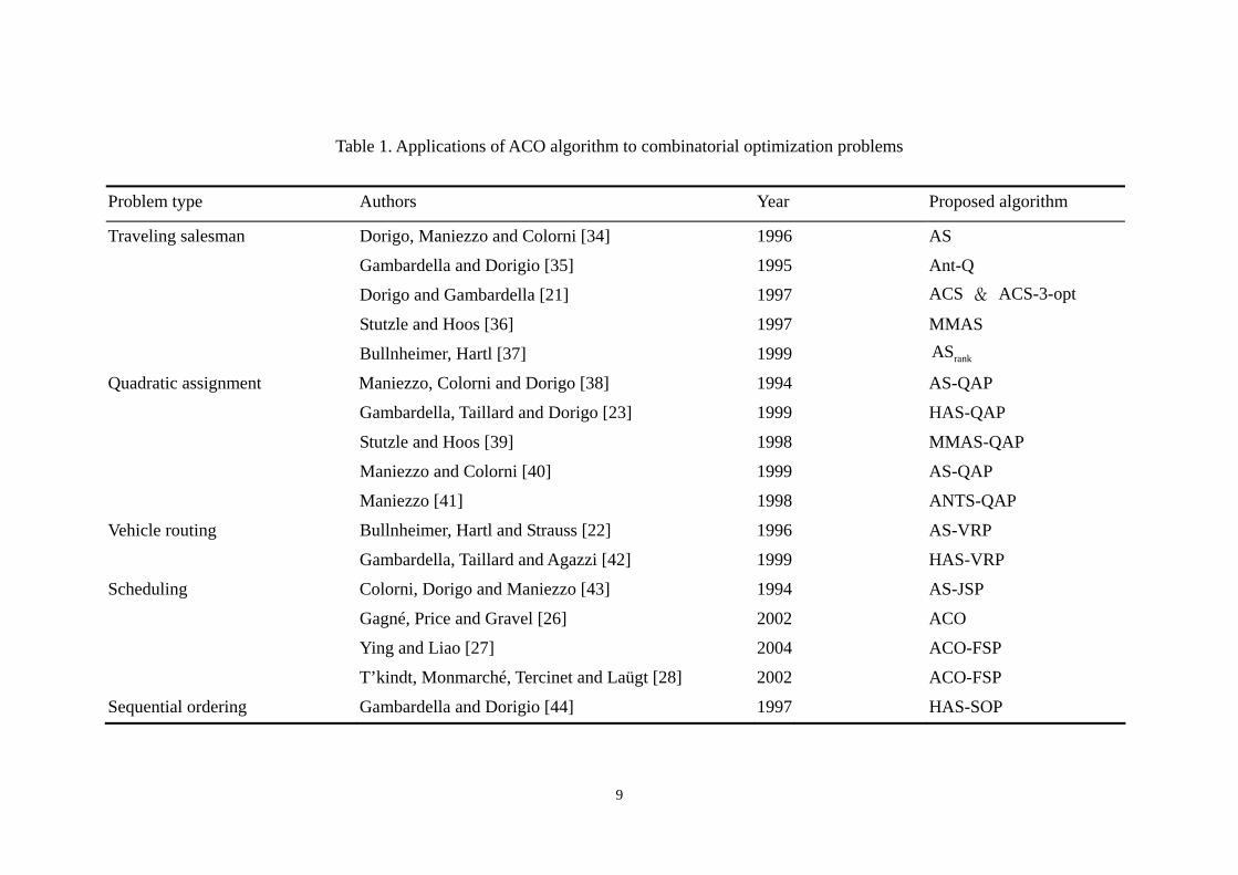
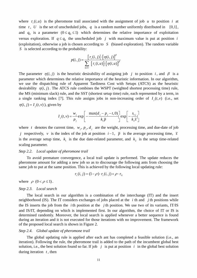
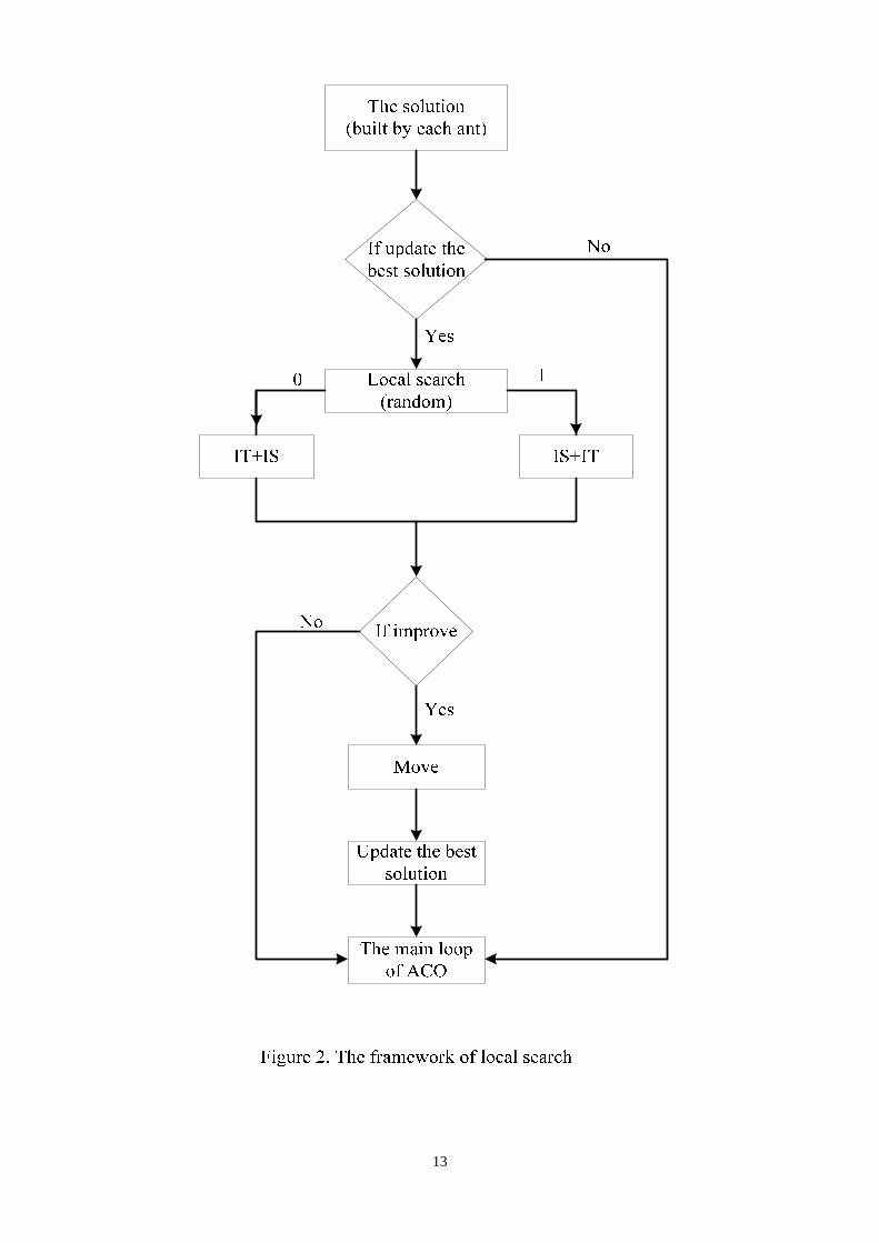
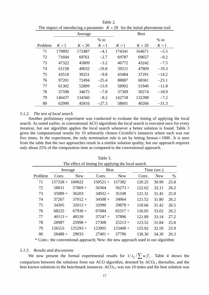
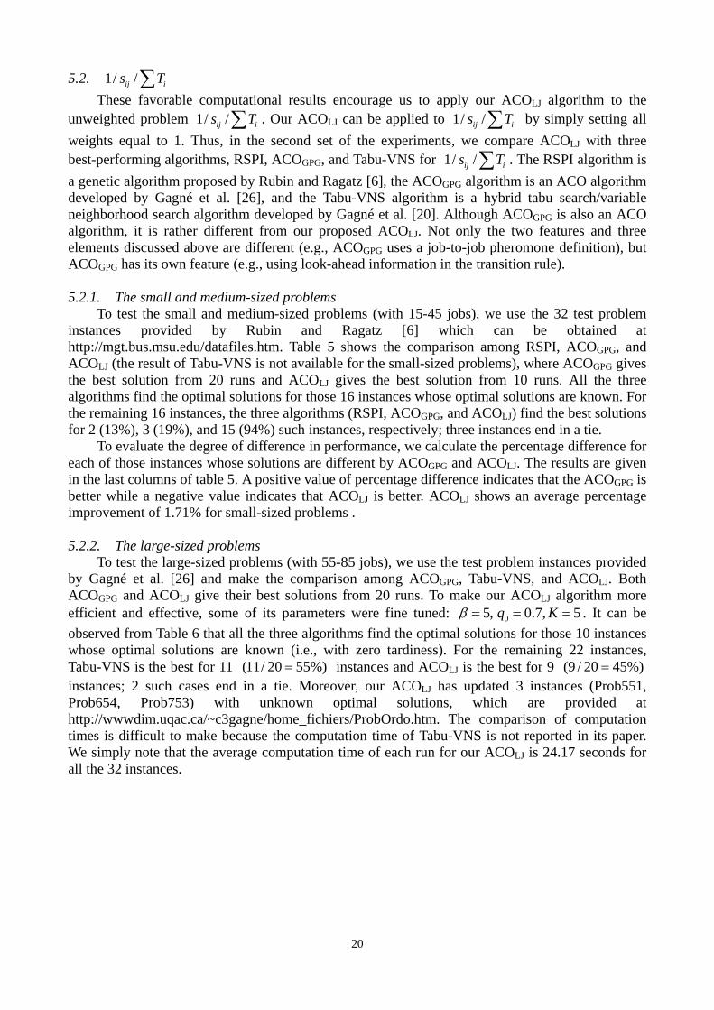
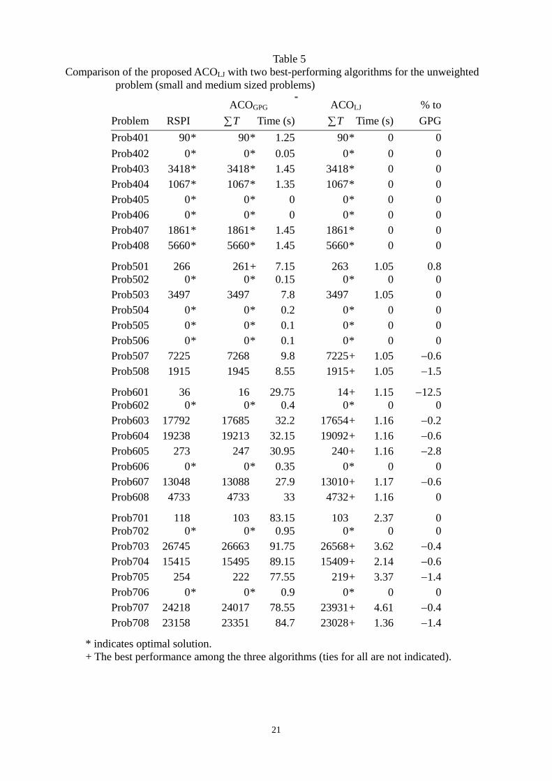
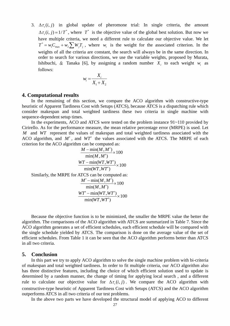
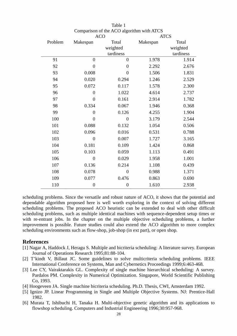
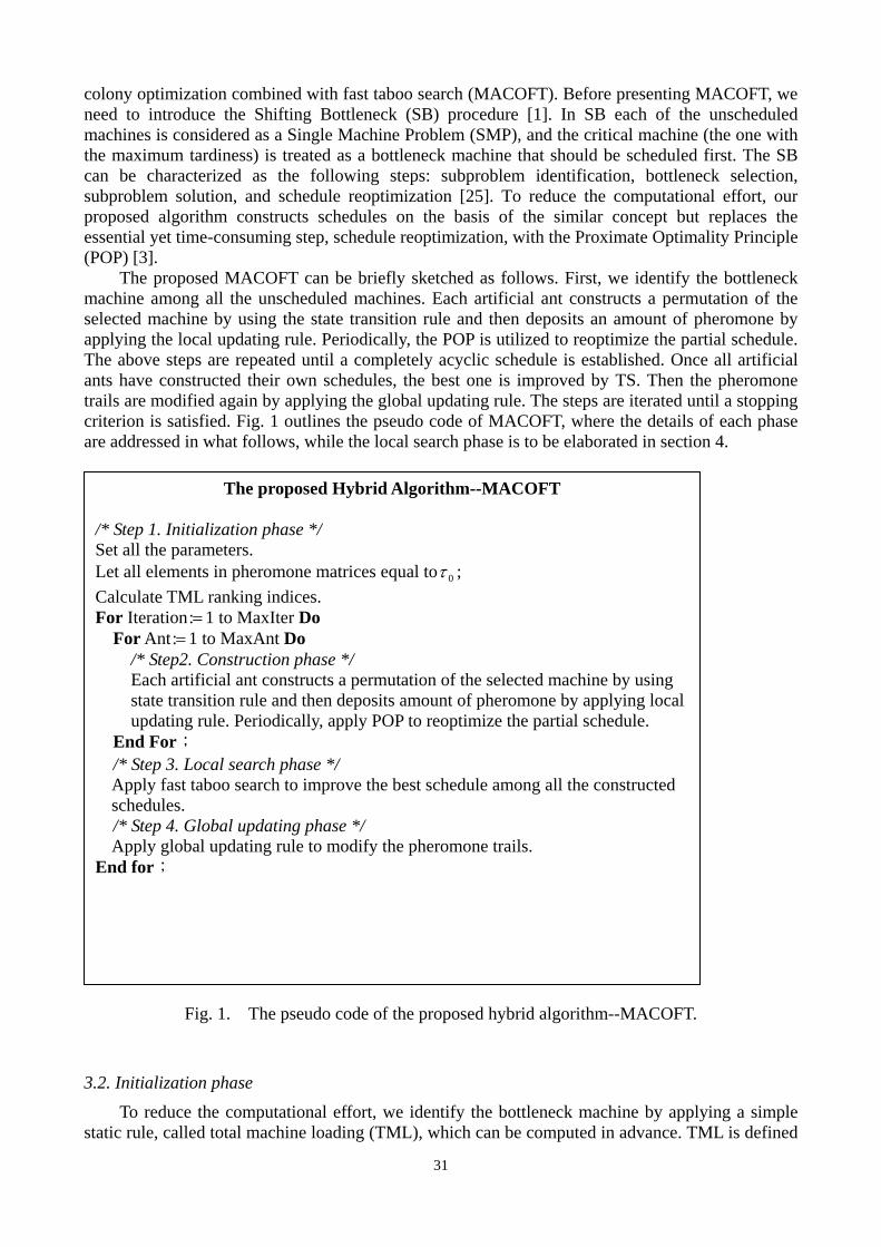
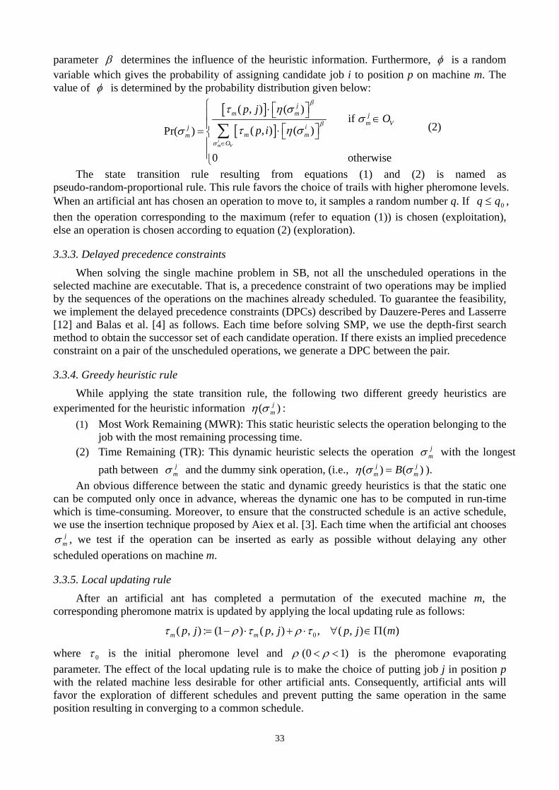
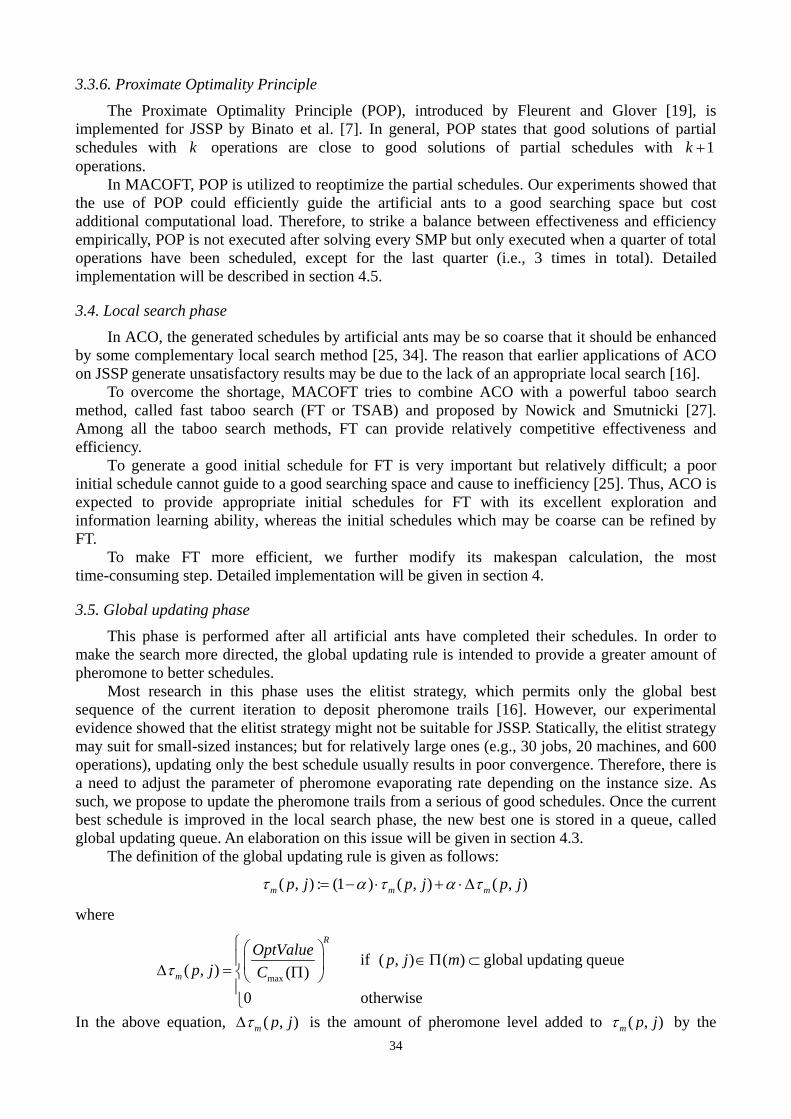
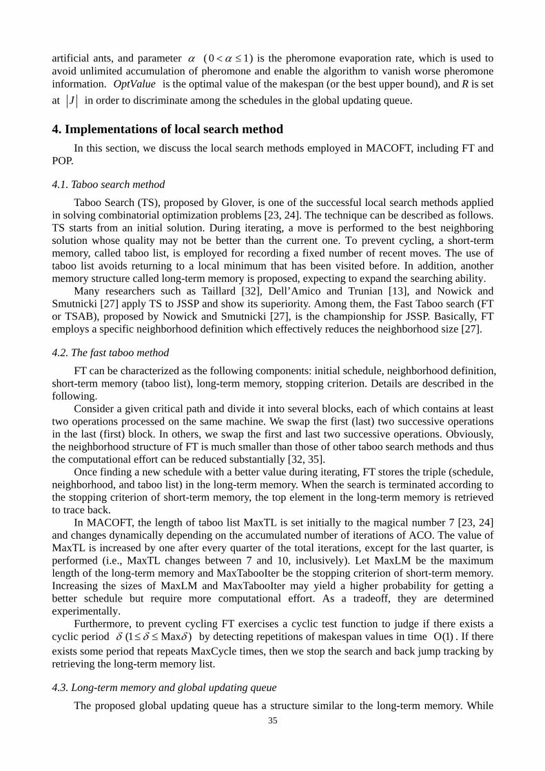
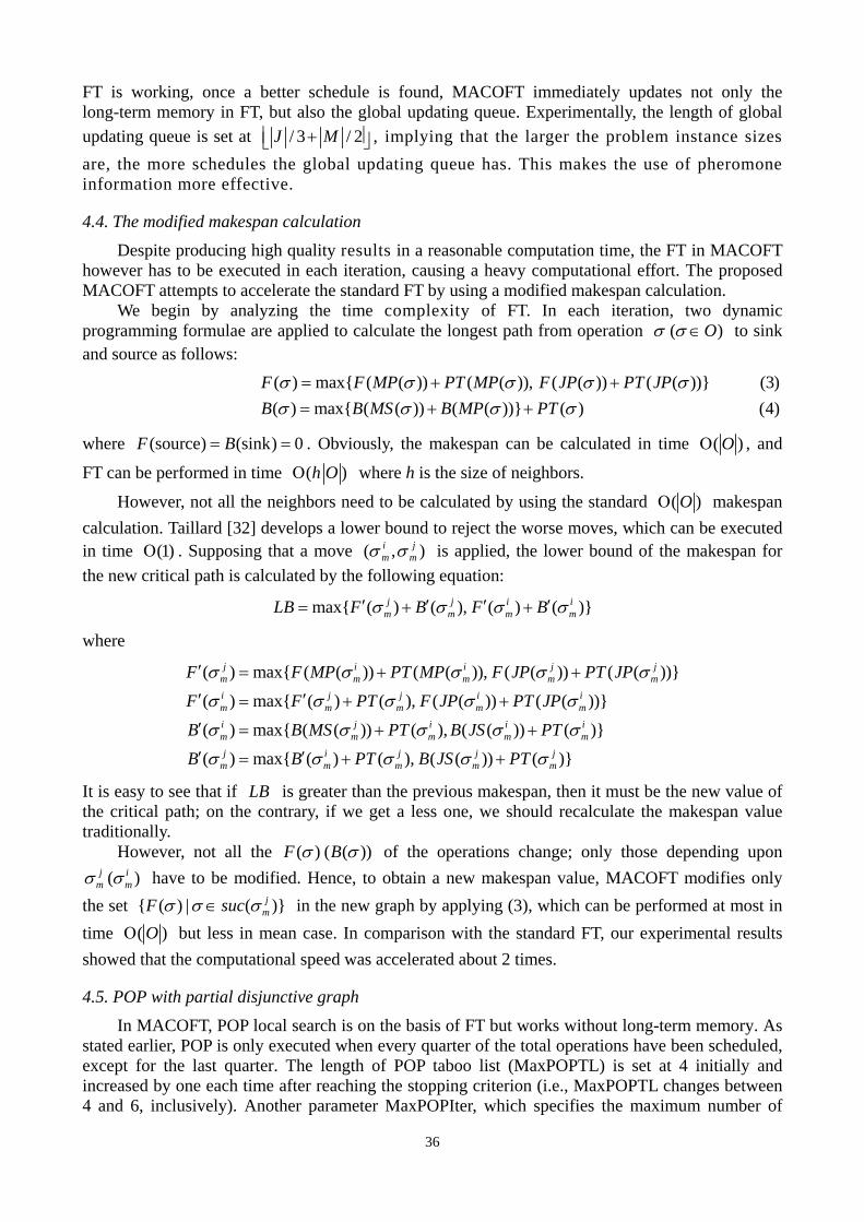
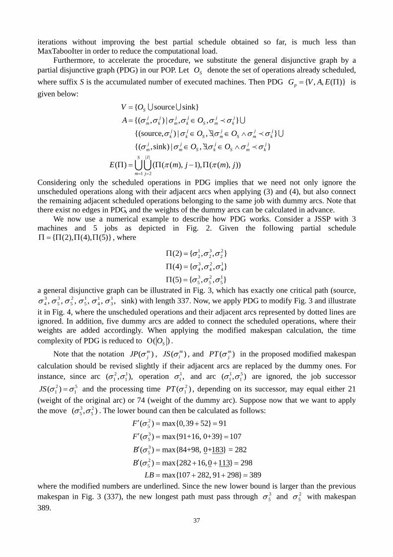