Environmental Science & Policy 54 (2015) 268–280

Mapping green infrastructure based on ecosystem servicesand ecological networks: A Pan-European case study

Camino Liquete a,b,*, Stefan Kleeschulte b, Gorm Dige c, Joachim Maes d, Bruna Grizzetti a,Branislav Olah e, Grazia Zulian d

a European Commission, Joint Research Centre (JRC), Institute for Environment and Sustainability (IES), Water Resources Unit, Via Enrico Fermi 2749, 21027

Ispra, VA, Italyb GeoVille Environmental Services, 3 Z.I. Bombicht, L-6947 Niederanven, Luxembourgc European Environment Agency, Natural Systems and Vulnerability, Kongens Nytorv 6, 1050 Copenhagen K, Denmarkd European Commission, Joint Research Centre (JRC), Institute for Environment and Sustainability (IES), Sustainability Assessment Unit, Via Enrico Fermi 2749,

21027 Ispra, VA, Italye Technical University in Zvolen, Faculty of Ecology and Environmental Sciences, Department of Applied Ecology, Masaryka 24, 96053 Zvolen, Slovakia

A R T I C L E I N F O

Article history:

Received 9 March 2015

Received in revised form 26 June 2015

Accepted 9 July 2015

Keywords:

Green infrastructure

Ecosystem service

Habitat modelling

Connectivity

Prioritization

Conservation

Restoration

Europe

A B S T R A C T

Identifying, promoting and preserving a strategically planned green infrastructure (GI) network can

provide ecological, economic and social benefits. It has also become a priority for the planning and

decision-making process in sectors such as conservation, (land) resource efficiency, agriculture, forestry

or urban development.

In this paper we propose a methodology that can be used to identify and map GI elements at

landscape level based on the notions of ecological connectivity, multi-functionality of ecosystems and

maximisation of benefits both for humans and for natural conservation. Our approach implies, first, the

quantification and mapping of the natural capacity to deliver ecosystem services and, secondly, the

identification of core habitats and wildlife corridors for biota. All this information is integrated and

finally classified in a two-level GI network. The methodology is replicable and flexible (it can be tailored

to the objectives and priorities of the practitioners); and it can be used at different spatial scales for

research, planning or policy implementation.

The method is applied in a continental scale analysis covering the EU-27 territory, taking into account

the delivery of eight regulating and maintenance ecosystem services and the requirements of large

mammals’ populations. The best performing areas for ecosystem services and/or natural habitat

provision cover 23% of Europe and are classified as the core GI network. Another 16% of the study area

with relatively good ecological performance is classified as the subsidiary GI network. There are large

differences in the coverage of the GI network among countries ranging from 73% of the territory in

Estonia to 6% in Cyprus. A potential application of these results is the implementation of the EU

Biodiversity Strategy, assuming that the core GI network might be crucial to maintain biodiversity and

natural capital and, thus, should be conserved; while the subsidiary network could be restored to

increase both the ecological and social resilience. This kind of GI analysis could be also included in the

negotiations of the European Regional Development Funds or the Rural Development Programmes.

� 2015 The Authors. Published by Elsevier Ltd. This is an open access article under the CC BY license

(http://creativecommons.org/licenses/by/4.0/).

Contents lists available at ScienceDirect

Environmental Science & Policy

jo u rn al ho m epag e: ww w.els evier . c om / lo cat e/en vs c i

* Corresponding author. Present address: European Commission, Joint Research

Centre (JRC), Institute for Environment and Sustainability (IES), Water Resources

Unit, Via Enrico Fermi 2749, TP 121, 21027 Ispra, VA, Italy.

E-mail addresses: camino.liquete@jrc.ec.europa.eu, camino.liquete@gmail.com

(C. Liquete), kleeschulte@geoville.com (S. Kleeschulte), gorm.dige@eea.europa.eu

(G. Dige), joachim.maes@jrc.ec.europa.eu (J. Maes),

bruna.grizzetti@jrc.ec.europa.eu (B. Grizzetti), olah@tuzvo.sk (B. Olah),

grazia.zulian@jrc.ec.europa.eu (G. Zulian).

http://dx.doi.org/10.1016/j.envsci.2015.07.009

1462-9011/� 2015 The Authors. Published by Elsevier Ltd. This is an open access artic

1. Introduction

Many aspects of human wellbeing and economic activities relyon ecosystem functions and processes. For instance, our foodsecurity is based on the existence and maintenance of fertile soil;we breathe the air that plants filter; our lives and properties areprotected from flooding by soil infiltration, dune systems orriparian forests; and our mental and physical health may depend

le under the CC BY license (http://creativecommons.org/licenses/by/4.0/).

C. Liquete et al. / Environmental Science & Policy 54 (2015) 268–280 269

on the accessibility to green spaces (MA, 2005; Alcock et al., 2014).Furthermore, some nature-based technical solutions (e.g. greenroofs, bio-infiltration rain gardens, vegetation in street canyons)have demonstrated in several cases to be more efficient,inexpensive, adaptable and long-lasting than the so-called ‘‘grey’’or conventional infrastructure (e.g. Gill et al., 2007; Pugh et al.,2012; Ellis, 2013; Flynn and Traver, 2013; Raje et al., 2013).

The European Commission communication (2013) on greeninfrastructure (GI) sets the ground for a tool that aims to provideecological, economic and social benefits through natural solutions,helping us to mobilise investments that sustain and enhance thosebenefits. This vision pursues the use of natural solutions(considered multi-functional and more sustainable economicallyand socially) in contrast with grey infrastructure (that typicallyonly fulfils single functions such as drainage or transport). In the ECcommunication, GI is defined as a strategically planned network of

natural and semi-natural areas with other environmental features

designed and managed to deliver a wide range of ecosystem

services. This definition includes three important aspects: the ideaof a network of areas, the component of planning and manage-ment, and the concept of ecosystem services. In this sense, GIintegrates the notions of ecological connectivity, conservation andmulti-functionality of ecosystems (Mubareka et al., 2013).

In the European context, besides the abovementioned ECcommunication, the conservation and development of a GI isidentified as one of the priorities in EU policies covering a broadrange of sectors, like the EU Biodiversity Strategy to 2020,1 theroadmap to a Resource Efficient Europe,2 the Commission’sproposals for the Cohesion Fund and the European RegionalDevelopment Fund,3 the new Common Agricultural Policy4 (notethe change from direct payments towards the second pillarpayment that can be a strong incentive for GI restoration andmaintenance), the new EU Forest Strategy5 (especially relevantsince many GI elements might be forest-based), or the forthcomingcommunication on ‘‘land as a resource’’ in 2015 (which willhighlight the importance of using land efficiently and as a finiteresource). Within the Biodiversity Strategy, target 2 aims atmaintaining and restoring ecosystems and their services by 2020,by establishing a GI and restoring at least 15% of degradedecosystems. Action 6 is setting priorities to restore and promotethe use of GI. The forthcoming land communication will focus onthe value of land as a resource for crucial ecosystem services and onhow to deal with synergies and trade-offs between multiple landfunctions. Systematically including GI considerations in theplanning and decision-making process will help reduce the lossof ecosystem services associated with future land use changes (i.e.land take and land degradation) and help improve and restore soiland ecosystem functions.

To support the planning process, approaches for mapping GIare necessary. They should focus on two basic concepts. The firstone is multi-functionality, ensured by quantifying and mappinga number of ecosystem services. Decision makers can then seekfor areas providing multiple services. The second concept shouldbuild on connectivity analyses such as the analysis of ecological

1 COM (2011) 244 final, http://eur-lex.europa.eu/legal-content/EN/TXT/PDF/

?uri=CELEX:52011DC0244&from=EN.2 COM (2011) 571 final, http://ec.europa.eu/environment/resource_efficiency/

pdf/com2011_571.pdf.3 COM (2011) 612 final/2, http://www.espa.gr/elibrary/

Cohesion_Fund_2014_2020.pdf; COM (2011) 614 final, http://www.esparama.lt/

es_parama_pletra/failai/fm/failai/ES_paramos_ateitis/

20111018_ERDF_proposal_en.pdf.4 COM (2010) 672 final, http://eur-lex.europa.eu/LexUriServ/LexUriServ.

do?uri=COM:2010:0672:FIN:en:PDF; Regulations 1305/2013, 1306/2013, 1307/

2013 and 1308/2013.5 COM (2013) 659 final, http://eur-lex.europa.eu/LexUriServ/LexUriServ.

do?uri=COM:2013:0659:FIN:en:PDF.

networks. Spatial delineation of GI elements has often beenbased on a re-classification of available land cover datacombined with information on natural values of each coverclass (e.g. Weber et al., 2006; Wickham et al., 2010; Mubarekaet al., 2013). Recent studies have shown the relevance ofincluding sector specific models and connectivity in the analysisof policy impacts over GI networks (Mubareka et al., 2013). Inparticular, these authors find particularly relevant to forecastthe land claimed by the agricultural sector, population projec-tions, forestry and industry.

The objective of this paper is to propose a feasible andreplicable methodology to identify and prioritise GI elements,including the concepts of ecosystem services and ecologicalconnectivity. This methodology can be used at different spatialscales for planning and policy implementation. The proposedapproach is applied in a continental case study, covering the EU-27 territory, focusing on a landscape scale. In this case the resultscould be used for conservation policies since they are aligned withthe EC communication and the Biodiversity Strategy. This paper isa further refinement of a study started by EEA/ETC-SIA (EEA,2014).

2. The proposed methodology

2.1. Conceptual aspects: criteria to identify GI elements

As we anticipated in the introduction, this study is focused onthe identification of GI elements at landscape level. Unlike in urbanenvironments, in the open landscape not all green areas qualify asGI. It is not economically or technically feasible to cover the entireterritory with natural ecosystems in order to secure their positiveinfluence on natural processes on every spot. Hence, we consider ascrucial criteria to identify GI elements (i) the multi-functionalitylinked to the provision of a variety of ecosystem services, and (ii)the connectivity associated to the protection of ecologicalnetworks.

The first criterion, ecosystem services, are the contributionsof natural systems to human wellbeing. We propose that GIelements should be multi-functional zones in terms of services’delivery (EC, 2012). Moreover, we focus on the identification ofGI elements for conservation purposes, in line with one of theaims of GI in the EC Communication (2013): protecting and

enhancing nature and natural processes as a green alternative togrey infrastructure. We concentrate on the regulating andmaintenance services (as defined in Table 4 of Haines-Young andPotschin, 2013), since most of the provisioning and culturalservices are mainly driven by human inputs like energy (e.g.labour, fertilisers) or capital (e.g. touristic infrastructures), anddo not necessarily enhance natural processes (see trade-offanalysis and conclusions in Nelson et al., 2009; Maes et al.,2012). These concerns are further explained in section 5. Forexample, if we include food provision in the assessment and wehighlight the areas with a maximum production (crop yield) wewill probably spot intensive agriculture areas that are sustainedmore by human inputs, like fertilisers and mechanical means,than by nature, like soil organic matter. With the availableknowledge and information, by concentrating on regulating andmaintenance services, we can assume that an improvement onthe resulting GI network will enhance the condition of theecosystems and natural processes.

With these premises (protecting and enhancing nature andnatural processes), we decide to focus on the natural capacity oflandscapes to deliver services before taking into account thehuman demand. This natural capacity, also refer to as ‘‘ecosystemfunction’’ in the ecosystem services’ cascade framework (or‘‘pathway’’ in de Groot et al., 2010), depends on the biophysical

Fig. 1. Flowcharts representing the methodology proposed in this paper. The upper flowchart shows the general methodology followed to identify and map GI networks,

while the bottom part illustrates the specific steps applied in the Pan-European case study (see Section 3).

6 The Economics of Ecosystems and Biodiversity, http://www.teebweb.org/

resources/ecosystem-services/.7 Common International Classification of Ecosystem Services, http://cices.eu/.

C. Liquete et al. / Environmental Science & Policy 54 (2015) 268–280270

structures and processes, ultimately linked to the ecosystems’condition (Maes et al., 2013). For example, when assessing airquality regulation for GI we measure the natural capacity as thepotential of the existing vegetation to capture and remove airpollutants, instead of measuring the actual flux of pollutantscoming from anthropogenic sources and being trapped by naturalfeatures (which will depend on human pressures). We insist thatthese choices are based on the purpose of our study (biodiversityconservation); in a different context the selection of ecosystemservices or indicators may change while the application of ourmethodology remains invariable.

The second main criterion to design a GI is the existence andconnectivity of ecological networks. All biotic functional groupsneed core areas where they can find living space, nourishment,nursery and breeding zones. Hence, the presence of these vitalareas is crucial to maintain biodiversity. But the connectivity ofthose ecosystems is also a way to support genetic diversity and,thus, the viability and resilience of habitats and populations (Oldset al., 2012; Gibson et al., 2013; Ishiyama et al., 2014).Consequently, habitat modelling and ecological connectivity shallalso be included in the analysis of GI.

2.2. Technical aspects: mapping GI

We propose a mapping methodology that focuses on (i) thecapacity to deliver regulating and maintenance services, and (ii)the existence of core habitats for biota and the connectivity amongthose areas, as summarised in Fig. 1.

The first part of the assessment (upper branches of flowcharts inFig. 1) starts with the identification of relevant regulating andmaintenance ecosystem services for the study area. We recom-

mend following one of the established classifications of ecosystemservices such as TEEB6 or CICES.7

The following and most demanding step is to assess and mapthe select ecosystem services. There are several approaches to dothis (see review in Maes et al., 2012), from the direct conversion ofland use/land cover maps (e.g. Burkhard et al., 2009), through thecompilation of local primary data or statistics (e.g. Kandziora et al.,2013), to the application of dynamic process-based ecosystemmodels (e.g. Schroter et al., 2005). We prefer to identify and map agood proxy for the biophysical process responsible of eachecosystem service, if possible based on published scientific modelsand results. Each selected proxy should represent the naturalcapacity of ecosystems to deliver the correspondent service(service supply).

The next step is to normalise and integrate the data setsdescribing the ecosystem services. The selection of differentnormalisation methods and data thresholds will affect the finalresults, meaning that the user needs to consider what is the finalobjective before producing a map.

The second part of the assessment (lower branch of Fig. 1) is theidentification of core and transitional habitats for key functionalgroups. As core habitats and functional connectivity are species-related, the national/local authorities should identify their mostrelevant species. Based on field studies and/or models, practi-tioners should identify (a) the core habitats for those key species,and (b) perform a habitat connectivity analysis to identifypotential wildlife corridors, which requires expert knowledge

Table 1Selection of ecosystem services to define GI elements for the Pan-European case study. They are eight regulating and maintenance services linked to the CICES classification.

We provide for each service a specific name, a short definition and a spatially explicit proxy or indicator to quantify it. The specific data sets and models used to estimate those

proxies/indicators are detailed in Appendix.

Ecosystem services classification following CICES v4.3 Ecosystem services selected for this study

Section Division Group Selected service and short definition Selected proxy

Regulation and maintenance

ecosystem services

Mediation of waste,

toxics and other

nuisances

Mediation by

ecosystems

Air quality regulation: Potential of

ecosystems to capture and remove air

pollutants in the lower atmosphere.

Deposition velocity of air pollutants

on vegetation (based on Pistocchi

et al., 2010)

Mediation of flows Mass flows Erosion protection: Potential of

ecosystems to retain soil and to

prevent erosion and landslides.

Erosion control (Maes et al., 2011)

Liquid flows Water flow regulation: Influence

ecosystems have on the timing and

magnitude of water runoff and

aquifer recharge, particularly in

terms of water storage potential.

Water infiltration (Wriedt and

Bouraoui, 2009)

Coastal protection: Natural defence of

the coastal zone against inundation

and erosion from waves, storms or

sea level rise.

Coastal protection capacity

(Liquete et al., 2013)

Maintenance of

physical, chemical,

biological conditions

Lifecycle maintenance,

habitat and gene

pool protection

Pollination: Potential of animal

vectors (bees being the dominant

taxon) to transport pollen between

flower parts.

Relative pollination potential

(Zulian et al., 2013)

Soil formation and

composition

Maintenance of soil structure and

quality: The role ecosystems play in

sustaining the soil’s biological

activity, physical structure,

composition, diversity and

productivity.

Theoretical ecosystem potential

(Kleeschulte et al., 2012)

Water conditions Water purification: The role of biota in

biochemical and physicochemical

processes involved in the removal of

wastes and pollutants from the

aquatic environment.

In-stream nitrogen retention

efficiency (Grizzetti et al., 2012)

Atmospheric composition

and climate regulation

Climate regulation: The influence

ecosystems have on global climate by

regulating greenhouse and climate

active gases (notably carbon dioxide)

from the atmosphere.

Carbon stocks from the carbon

accounts (Simon Colina et al., 2012)

C. Liquete et al. / Environmental Science & Policy 54 (2015) 268–280 271

and interpretation. We can recommend the use of tools such asLinkage Mapper Connectivity Analysis Software8 or GuidosTool-box9 that can be tailored for any scale and species. The spatialresults of this habitat suitability analysis must be normalised andintegrated in a similar way as the ecosystem services’ maps.

The results of the two assessments are made comparable usinga ranking normalisation method and are then integrated. In thisintegration the highest value (the best performing result eitherlinked to ecological connectivity OR to ecosystem services) shouldsupersede the other. We underline here ‘‘or’’ because it is not acombination of functions, but the selection of the best performingone. Thus, we propose a selection of maximum values in a pixel-by-pixel basis. Lastly, the results are classified as follows:

� The GI core network with maximum values of the integratedresults (the highest capacity to provide ecosystem services and/or key habitats for biota);� The GI subsidiary network with moderate values of the

integrated results.

The thresholds used to define the maximum and moderatecategories will affect the final distribution of results and the totalcoverage of the resulting GI network and, thus, should be linked tothe management priorities and requirements of the study.Multiple outputs can be generated and compared before the final

8 http://www.circuitscape.org/linkagemapper.9 http://forest.jrc.ec.europa.eu/download/software/guidos/.

decision is taken, especially when the decision process involvesseveral stakeholders.

This entire methodology is designed as a flexible and replicableprocedure that should be tuned up for each regional study. Thereare three steps at which the user may decide to adjust it (Fig. 1): (1)in the initial selection of ecosystem services and functional groupsto assess; (2) in the normalisation of original values, selecting thedata distribution and limits between classes; and (3) in the finaldefinition of GI categories, balancing the optional thresholds withthe resulting GI network and the feedback from the interestgroups.

3. The Pan-European case study

3.1. Ecosystem services in Europe

We selected eight regulating and maintenance ecosystemservices and we compiled or adapted spatially explicit informationabout the capacity to deliver each of them in EU-27 (Croatia couldnot be covered due to lack of data) (Table 1). Since the formats andspatial units of each model were different, all input data weretransformed into grids of 1 km spatial resolution.

In the Pan-European case study, we opt for a normalisation ofeach input map based on minimum and maximum values. Thenormalised values and maps of the eight ecosystems services areshown in Fig. 2.

A full description of the ecosystem functions and biophysicalmodels used to map each ecosystem service is available in the

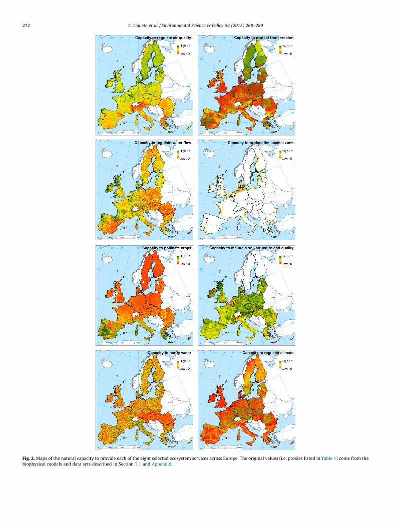
Fig. 2. Maps of the natural capacity to provide each of the eight selected ecosystem services across Europe. The original values (i.e. proxies listed in Table 1) come from the

biophysical models and data sets described in Section 3.1 and Appendix.

C. Liquete et al. / Environmental Science & Policy 54 (2015) 268–280272

C. Liquete et al. / Environmental Science & Policy 54 (2015) 268–280 273

Appendix. The Appendix also includes models’ design, assump-tions and input parameters as well as references to find the originalresults and interpretation. Here, we present a summary of theresults at European scale.

- Air quality regulation: the potential dry deposition velocity ofatmospheric pollutants across Europe ranges between 0.2 and1.2 cm/s. Minimum values are concentrated in most of Romania,Bulgaria, Greece, Italy, eastern Spain and around the Alpine arc.Maximum values are scattered around the Baltic and North Seashores, Ireland and NW Spain, W Portugal and some Greekislands. This is mostly linked to wind patterns and vegetal cover,both increasing towards the North or the Atlantic shores.

- Erosion protection: the erosion control indicator for Europe was adimensionless indicator ranging from 1 to 5 before normal-isation. Minimum values are widespread in continental Europeand the British Isles while maximum values are mostly found insouthern Finland, southern Sweden, SW Iberia, SW France andscattered locations of Latvia, Lithuania, Poland, Germany,Denmark and Greece. The maximum values highlight areas withrelatively high erosion risk and dense vegetal cover able to bindsoil particles or reduce wind/water speed.

- Water flow regulation: the total infiltration of water in the soilfluctuates between nearly 0 and 1116 mm/yr. The lowest valuesare usually concentrated in eastern Spain, southern Italy and thelower Danube. The few basins with peak values (more than700 mm/yr in the original data) are distributed in the BritishIslands, the NW Iberian Peninsula, and some Pyrenees and Alpinelocations. Climatic factors (e.g. precipitation) play a major role onthis distribution, but soil characteristics also affect the results.

- Coastal protection (dimensionless): relatively low coastal protec-tion capacity (close to 0) is present along the shores of Denmark,Germany, The Netherlands, some UK estuaries and the Gulf ofLion. Relatively high values (close to 1) are observed inScandinavian mid-latitudes, Scotland, Ireland, NW Spain, Corsicaand parts of Greece. These results are mainly driven by coastalgeomorphology and topography and, to a lesser extent, by thepresence of protective submarine and emerged habitats (e.g.biogenic reefs, dune systems).

- Pollination (dimensionless): the indicator on pollination potentialwas already normalised between 0 and 1. In general, minimumvalues tend to accumulate in northern Europe while maximumvalues appear in the Mediterranean region. These differences atcontinental scale are driven by the location of foraging andnesting sites and the effect of the insect activity index, whichdepends on temperature and solar irradiance. The location offoraging and nesting sites is impacted by human activities, whichare reflected in the land-use/land cover maps introduced in themodel.

- Maintenance of soil structure and quality (dimensionless): theoriginal values of this indicator ranged between 2 and 12. Thebest soil ecosystem potential is usually present in relativelyunpopulated areas across Europe with a particularly highconcentration in Austria and Scotland. The worst soil character-istics are equally scattered along EU-27 but show some patchesin western Ireland, northern Italy, the Danube delta, Crete andother Greek islands. Sweden and Finland are not covered by thisindicator.

- Water purification: the in-stream retention efficiency of nitrogen(by sub-catchment) ranges from nearly 0 to 16%. The relativelylow values in the Danube watershed are probably linked to thecalibration of the GREEN model, which was performed by majorEuropean seas’ drainage basins (Grizzetti et al., 2012), and by thefact that in-stream nitrogen tends to be conserved (notprocessed) in larger rivers (Alexander et al., 2000). Italy showsthe largest national average retention efficiency.

- Climate regulation: the estimated carbon content of above-ground biomass in EU terrestrial ecosystems ranges between0 and 20,004 tonnes of carbon per square kilometre, and it ismostly concentrated in forested areas. Countries with mini-mum above-ground biomass values are Ireland, Netherlands,Malta and UK. The Member States with the highest proportionof maximum carbon stock are the Czech Republic andAustria.

All these indicators (Fig. 2) are then combined through anarithmetic mean, in which the highest values represent the highestcombined capacity to deliver regulating and maintenance servicesacross EU-27. In order to combine these results with the secondpart of the methodology, which provides categorical data, wereclassify the average ecosystem service data into five ranksranging from minimum (1) to maximum capacity (5), based on anatural breaks’ distribution (Fig. 3A). Using the natural breaks’distribution for ranking works well for comparison purposes, likein this continental scale assessment. The areas with maximumcapacity (greenish colours) are assumed to perform key ecologicalroles both for wildlife and for the human well-being. The areaswith moderate capacity (yellowish colours) are performingimportant ecosystem functions but with a reduced or limitedpotential. In the reddish areas the ecosystem functions thatsupport services are minor, either because their natural structuredoes not allow for a higher potential or because the habitats aredeteriorated (for example a sparsely vegetated land when it refersto erosion protection, or an urban setting when it refers to climateregulation).

Our map 3A largely corresponds with the results from Maeset al. (2014, Fig. 3). The aggregation at regional level performed byMaes et al. obviously dilute some of the hot and coldspots found inour data, especially in the largest regions (e.g. our minimum valuesobserved in Spain). But when we aggregate our results to the samescale, the relative distribution of values is in line with thoseauthors. The largest regional discrepancies are found in Scandi-navia. Data from Schulp et al. (2014, Fig. 3 bottom right) is moredifficult to compare with our results, but the distribution ofminimum and maximum values per region seems to broadly agree,again with the larger differences in Scandinavia. However, thedifferent coverage of our maps affects the relative scale for thecomparison.

3.2. Habitat modelling and functional connectivity

We analysed the presence of essential habitats (core andtemporal habitats) for a selected functional group. In this case,being a continental scale analysis at 1 km resolution, we select thelarge mammals as focal group. Large mammals normally have highdemands in terms of habitat area and are able to cover largemigration distances. The parameters, data sources, species andmodels used to derive the presence of core habitats andconnectivity among them are detailed in Appendix.

The main results from the habitat modelling are the identifica-tion of 67 actual core habitats (i.e. core habitats in which thepresence of large mammals has been reported by EU MemberStates) and 53 extra potential core habitats (i.e. habitats suitablefor mammalian wildlife but without reported presence). Thehabitat connectivity analysis highlighted 91 corridor swathsconnecting the actual core areas or 156 linking all core habitats.These results refer to the European territory including all theBalkan countries (Fig. 3B).

The habitat modelling results are qualitative (i.e. presence orabsence of different kinds of habitats). Using the same scale as inthe ecosystem services’ normalisation (ranks from 1 to 5), weassign the following categories (Fig. 3B):

Fig. 3. Results of the Pan-European case study. (A) Capacity to deliver regulating and maintenance ecosystem services. (B) Key habitats to maintain healthy large-mammal

populations. The results of (A) and (B) are normalised from value 1 (poor capacity for ecosystem services and habitat) to value 5 (maximum capacity for ecosystem services

and habitat). (C) Proposed GI network for Europe based on the integration of (A) and (B). The GI core network comprises the best functioning ecosystems, crucial to maintain

both natural life and natural capital. The GI subsidiary network covers other relevant areas sustaining ecosystem services and wildlife. The spatial data shown in these three

maps will be available through the Ecosystem Services Partnership visualisation tool (www.esp-mapping.net).

C. Liquete et al. / Environmental Science & Policy 54 (2015) 268–280274

- maximum value (5) to the actual core habitats- high value (4) to wildlife corridors or transitional habitats among

actual core habitats- moderate value (3) to other potential core areas and to the

potential wildlife corridors among them- minimum value (1) to the rest of the territory.

Following this method, countries like Estonia, Slovenia, Latviaand Austria have approximately half of their territory under core

habitats for large mammals, while others like Cyprus orDenmark have none. The analysis shows that 29 of the 91 actualcore habitats linkages are shorter than 10 km, that is, more than30% of the wildlife corridors are relatively feasible to beimplemented and protected. The connectivity among corehabitats for large mammals may enhance the genetic flowacross Europe, which is particularly important to helpspecies to adapt to climate change and other environmentalalterations.

C. Liquete et al. / Environmental Science & Policy 54 (2015) 268–280 275

3.3. Towards a Pan-European GI network

The normalised results from ecosystem services (Fig. 3A) andhabitat modelling (Fig. 3B) are finally integrated based on aselection of maximum values, i.e. each square kilometre will takethe value of the criteria for which it is ecologically more important.This information is then transformed into an interpreted networkof GI for Europe divided in two categories (Fig. 3C).

In this case the core GI network (see explanation in Section 2.2)includes areas where the integrated ecosystem service capacityand habitat modelling take value 5, thus including all the corehabitats together with the areas with maximum potential todeliver ecosystem services for humans. The subsidiary GI networkcorresponds to value 4, where we find the wildlife corridors andwhere the provision of ecosystem services is above the average butnot optimal. The thresholds fixed to define these two types of GInetwork are variable and adaptable to the case study objectives;they should take into account the ecological and land-use planningrequirements.

The results illustrated in Fig. 3C indicate that 23% of the EU-27territory might be part of the core GI network and 16% of thesubsidiary GI network. The rest of the European territory did notqualify to form part of these GI networks. With the specificthresholds and criteria used in this case study, Estonia, Sloveniaand Latvia show the maximum coverage of core GI network(between 56 and 63% of their territory) while Malta, Cyprus andHungary show the minimum one (less than 2%). Regarding thesubsidiary GI network, Portugal and Greece have the largestcoverage (38 and 34% respectively). All in all Cyprus hasproportionally the smallest GI network (6% of its territory) andEstonia the largest one (73%).

The extension of the GI network proposed in map 3C issignificantly smaller than the results from Mubareka et al. (2013,Fig. 5) but the distribution is quite similar. Those authors follow afix land cover typology to identify GI elements. Both approacheshighlight mainly the large mountain ranges and densely forestedareas, while Mubareka and colleagues include also more sparseforests and even semi-natural vegetation, magnifying the differ-ences in the British-Irish Isles, Corsica, the Netherlands andScandinavia.

4. Applications of the identification of GI networks

An environmental focus of GI is fundamental to secure itsobjectives (Wright, 2011) but it is not enough. What defines GI isthe inclusion of goals for protecting ecological functions alongsidegoals for providing benefits to humans (McDonald et al., 2005). Oneof the strong points of the methodology proposed in this paper, andapplied across Europe, is the prioritisation of the ‘‘green’’ (rural)spaces to form part of a coherent, multi-functional GI network thatmaximises the potential benefits both for humans and for naturalconservation. The design of this methodology (Fig. 1) follows somecrucial GI principles such as contribute to biodiversity conserva-tion and enhance ecosystem services (Naumann et al., 2011). Thisthoroughly designed GI network could serve as an ecologicalbackbone of the landscape supporting natural processes andecosystem services in its surroundings.

Our proposal of two levels of GI networks (core and subsidiary)implies that biodiversity and the provision of ecosystem servicescan be not only protected but also improved (Rey-Benayas et al.,2009):

� The core GI network is generally related to the best condition ofthe ecosystems’ structures and processes. These areas are crucialto maintain biodiversity and natural capital and, thus, should bepreserved.

� In the subsidiary GI network ecosystem functions are stillimportant, but they could be probably upgraded to the core GInetwork to increase both the ecological and social resilience.Hence, they represent areas with a potential for restoration.

Some of the grey areas in Fig. 3 may be other kind of ‘‘green’’landscape providing other kind of services, like for instanceagricultural or semi-natural areas. They may have a high demandof GI and, thus, be candidates for building new GI elements (i.e.restoration), but this should be analysed individually in moredetail. The selection of priority areas should be settled at theappropriate management scale.

The European Biodiversity Strategy calls for establishing andpromoting the use of GI, and restoring at least 15% of degradedecosystems. Our results could be translated into the frameworkrecently proposed by the Working Group on a RestorationPrioritisation Framework, which looks into the best ways toimplement action 6 target 2 of the Biodiversity Strategy. Thisframework divides the continuum of ecosystem conditions frompoor to excellent into four distinct levels (Lammerant et al., 2013).After an appropriate ecological analysis of thresholds in the studyarea, the core GI network could be ascribed to level 1 of the 4-levelconcept for restoration, where ecosystems’ condition and theirfunctions are in good to excellent condition. The protection orconservation of these zones may guarantee the delivery ofecosystem services and the maintenance of species and popula-tions. It should be taken into account that, with our methodology,the proposed European GI network is not including all theprotected areas and natural parks that should probably take partof level 1, like the Lemmenjoki or the Pallas-Yllastunturi NationalParks in northern Finland for example. The subsidiary GI networkcould correspond to level 2, where abiotic conditions aresatisfactory but some ecological processes and functions aredisrupted with negative consequences in diversity. The ecosystemfunctions and, thus, the benefits from these zones could be boostedby some restoration actions. Hence, our methodology, onceadapted to the regional characteristics, can serve countries andlocal agencies to set priority areas for GI and to identify potentialareas for conservation and restoration. This can contribute to setup compatible Pan-European and national approaches to GI, bothconceptually and spatially. Future applications of this approachshall serve to aggregate and compare national GI delineations withEuropean ones (through up-scaling or nesting scales approaches).

This ecologically based GI network could be combined with otherEU social and economic policies since they all address territoriallydependent issues as human well-being, nature conservation orterritorial cohesion and are based on a geographical concept. Hencethe GI network could be included in the negotiations of the EuropeanRegional Development Funds under the EU cohesion policy 2014–2020 or the regional Rural Development Programmes under the EUrural development policy 2014–2020.

The methodology proposed in this article can be applied forother scientific uses such as the identification of data andknowledge gaps (e.g. unknown quantification of certain ecosystemservices), the establishment of specific local/regional thresholdsand criteria (e.g. definition of maximum capacity, or limits forhabitat suitability for local species), the valuation of alternativeoptions (e.g. cost-benefit or cost-efficiency analysis of a certain GIelement), or the suitability of conservation zones linked to GI interms of protected areas or endangered species (e.g. comparison ofNatura 2000 zones with different GI networks), among others.

5. Main challenges and future steps

There are several sources of uncertainty that may affect theresults of the Pan-European case study. Based on the suggestions of

C. Liquete et al. / Environmental Science & Policy 54 (2015) 268–280276

Hou et al. (2013) and Schulp et al. (2014), the main sources ofuncertainty of our analysis can be summarised as follows:

- Natural supply uncertainty, linked to the complexity andvariability of ecosystem functions and species. In this casepotential sources of uncertainty are:� The (lack of) knowledge and understanding of the biophysical

processes and species behaviour� The selection and definition of the ecosystem services

indicators� Uncertain information related to land-use and land cover data,

dynamics and scale issues- Technical uncertainty, linked to the tools and methods applied

like:� Uncertainties based on model structure (assumptions, simpli-

fications and formulations) or input parameters� Inaccuracy of spatial data, mapping limitations, availability of

robust indicators, integration of data of varying quantity andquality� Selection of mapping and integrating methods

As we explained in Section 2.2 and illustrated in Fig. 1, ourmethodology can and should accommodate some case-specificoptions, from the selection of relevant ecosystem services andfunctional groups, to the establishment of thresholds. Theunevenly distributed results obtained across EU-27 Member Stateshighlight the need for such adaptation at national or regional level.The Pan-European case study was not designed to support themanagement of individual local sites, but the individual sites canbenefit from landscape approaches since they take into account thesite’s relationship and functional connectivity with wider habitatnetworks (Kettunen et al., 2007). The development of multi-scaleapproaches may enable up- or down-scaling and maintainingcompatibility with national or Pan-European approaches inrelation with biodiversity policies.

The proposed methodology could be enriched in various ways.For instance, in order to support decision-making, it is highlyrecommended to include the stakeholders’ involvement andfeedback in the first steps of GI design (McDonald et al., 2005;Hostetler et al., 2011). In this environmental approach we did notattempt to include participatory processes, socio-economicaspects or human population dynamics. All these factors couldbe considered for the design of GI. In particular, a step further onthis research should involve the integration of human demand forecosystem services as well as the delivery of provisioning andcultural services in a nature-protection GI network. When doing so,topics such as the sustainable flow of each service (e.g. themaximum level of delivery at which ecosystems are not degraded),the geographical and temporal distribution of demand (e.g. wherethe services and mainly produced and where are they consumed),the energy and capital inputs, or the conflicts and trade-offsbetween different ecosystem functions and human uses (Horwood,2011) should be taken into account.

Temporal variability could not be covered in this paper. However,ecosystems are not stable entities but continuously developingdynamic systems that provide services depending on their conditionduring each period. Also, transformations such as land use/landcover changes or climate change may have severe effects in thedistribution of suitable habitats for biota and GI elements. Atemporal assessment of ecosystems and ecosystem services couldhelp understand, analyse and even predict the GI evolution.

6. Conclusions

GI is evaluated in this paper as an ecological and spatial conceptthat has the aim to promote ecosystems’ health and resilience,

contribute to biodiversity conservation and, at the same time,provide benefits to humans promoting the multiple delivery ofecosystem services. The multi-functionality of GI is the backboneof this analysis and is addressed by considering ecosystemsservices, provision of core habitats to biota and ecologicalconnectivity.

In this paper we propose a methodology to identify and mapGI networks at landscape level and we apply it in a Pan-European case study. This approach is based on (1) thequantification of the natural capacity to deliver ecosystemservices, (2) the identification of essential core habitats andcorridors for wildlife, and (3) the integration of all thatinformation into a meaningful network of GI. That GI networkis divided in two categories that can help identifying potentialareas for conservation and/or restoration.

The methodology can be replicated at any other location andscale. One of its main advantages is its flexibility to adjust theselection criteria and data distribution (i.e. what is moreimportant in a particular setting), which will obviously affectthe final results.

Numerous policies, particularly those related to biologicalconservation, environment, cohesion and territory, may benefitfrom the definition and implementation of GI networks.

Conflict of interest

The authors declare no conflict of interest.

Acknowledgements

The scientific output expressed in this document does not implya policy position of the European Commission or other institutionsof the European Union.

This study was partially supported by EEA/ETC-SIA technicalreport No. 2/2014 – Spatial analysis of green infrastructure inEurope; by VEGA No. 1/0186/14 – Assessment of ecosystemservices at national, regional and local level; and by OpenNESS –Operationalisation of natural capital and ecosystem services: fromconcepts to real-world applications (grant agreement no. 308428).

Special thanks go to the two anonymous reviewers who revisedand made constructive comments on the manuscript.

Appendix. Data sources and models for the Pan-European casestudy

A.1. Air quality regulation

Forests, parks and other GI features can reduce pollution byabsorbing and filtering pollutants such as particulate matter.Pollutants can be removed from the atmosphere through deposi-tion or by conversion to other forms. The deposition of pollutantson the earth surface can be linked to dry deposition (mainlygaseous sulphur and nitrogen compounds) and wet depositionprocesses (namely aerosols and soluble gases). Direct deposition tovegetation (dry deposition) is an important pathway for cleaningthe lower atmosphere.

We select the dry deposition velocity on leaves as an indicatorof the capacity of ecosystems to capture and remove air pollutants,as proposed in previous studies (Escobedo and Nowak, 2009; Karlet al., 2010). Data for the year 2006 are re-estimated for this paperbased on the atmospheric particle deposition velocity of theMAPPE model (Multimedia Assessment of Pollutant Pathways inEurope, Pistocchi et al., 2010). MAPPE consists in a series ofspatially explicit models that simulate the pollutant pathways inair, soil and surface and sea water at the European scale (now

C. Liquete et al. / Environmental Science & Policy 54 (2015) 268–280 277

included in the FATE initiative http://fate.jrc.ec.europa.eu/rational/home).

The deposition velocity (DV) is a linear function of wind speedat 10 m height (w) and land cover type that can be noted as:

DVi ¼ a j þ b j � wi (1)

where a and b are, respectively, the intercept and slope coefficientscorresponding to each broad land cover type j (namely forest, baresoil, water or a combination of the previous) and i denotes thecalculation in each pixel.

A.2. Erosion protection

Bare soils offer no protection against wind and rain andrepresent a high risk of soil erosion, landslides, sedimentation instreams and rivers, clogging of waterways and land degradation.Accelerated soil erosion by water as a result of changed patternsin land use is a widespread problem in Europe. By removing themost fertile topsoil, erosion reduces soil productivity and, wheresoils are shallow, may lead to an irreversible loss of naturalfarmland. The capacity of natural ecosystems to control soilerosion is based on the ability of vegetation (i.e. the rootsystems) to bind soil particles and to reduce wind/water speed,thus preventing the fertile topsoil from being blown or washedaway by water or wind.

The procedure to map erosion control is based on Maes et al.(2011). The MESALES model from the European Soil DataCentre10 analyses data on land use, slope, soil properties andclimate (wind and precipitation) to predict the seasonal andannual averaged soil erosion risk. The resulting map on soilerodibility categorises soils into five risk classes (very low, low,medium, high and very high sensitivity to erosion). Next, the soilerodibility map was intersected with a map of naturalvegetation based on the Corine Land Cover (CLC2000) dataset.Polygons resulting from the intersection between naturalvegetation and soil erodibility received a score between 1 and5 depending on the soil erosion risk class. This procedure givesmore weight to natural vegetation in areas where erosion risk ishigh. The final indicator is the weighted surface area share ofnatural vegetation in each 1 km grid cell. This procedure usesthe CLC data twice, but as a consequence of the scale differencebetween the erodibilty map and the map of natural vegetation, itresults in a map of protective vegetation on soils with a high riskfor erosion.

A.3. Water flow regulation

The flow regulation function refers to the ability of watershedsto capture and store water from rainfall events (Le Maitre et al.,2014) in contrast with artificial impervious surfaces. The influenceof soil and vegetation on the timing and magnitude of water runoffhas numerous positive effects such as regulate flood events, andrecharge slowly the groundwater, maintaining the baseflow ofstreams. Water infiltration and percolation through the soil are keyprocesses in flow regulation.

We use the annual infiltration (F, mm/yr) estimated by Wriedtand Bouraoui (2009) based on the modelling approach suggestedby Pistocchi et al. (2008), as an indicator of the capacity ofterrestrial ecosystems to temporarily store and regulate waterflow. This annual infiltration represents the water available forslow and fast subsurface runoff (QSSF), i.e. for groundwater andinterflow, and it is estimated as difference between (effective)

10 http://eusoils.jrc.ec.europa.eu/ESDB_Archive/serae/GRIMM/erosion/inra/

europe/analysis/maps_and_listings/web_erosion/index.html.

precipitation (P) and actual evapotranspiration (ETA) and runoff(RO).

FðtÞ ¼ PðtÞ � ETAðtÞ � ROðtÞ (2)

QSSFðtÞ ¼ ðFðtÞjFðtÞ � 0Þ (3)

where runoff (RO) is represented as a function of precipitation,in the form of a combination of an SCS (Soil ConservationService) curve number model and a linear runoff model withrunoff coefficient, and the actual evapotranspiration (ETA) isestimated by the formula proposed by Turc (1955) (Pistocchiet al., 2008).

Thus, the estimation of annual infiltration used in this study isbased on climatic factors (precipitation and evapotranspiration)and the soil water holding potential (the soil type and textureaffecting RO).

A.4. Coastal protection

Coastal protection can be defined as the natural defenceof the coastal zone against inundation and erosion fromwaves, storms or sea level rise. Habitats (e.g. wetlands, dunes,seagrass meadows) and other environmental features (e.g. cliffs,enclosed bays) act as physical barriers protecting any asset orpopulation present in the coastal zone. In many locations, theseecosystems suffer from increasing pressure from expandinghuman populations and from a lack of long-term coastalmanagement. This ecosystem service includes several processeslike attenuation of wave energy, flood regulation, erosioncontrol or sediment retention. The consequence of naturalhazards on the coastal zone and their impacts on humans(usually referred to as coastal vulnerability) is a topic of highinterest for science, society and policy-making alike (e.g. Adgeret al., 2005).

Liquete et al. (2013) developed a specific indicator for coastalprotection capacity (CP) defined as the natural potential thatcoastal ecosystems possess to protect the coast against inundationor erosion. We use the distribution of this indicator across Europeto represent the potential to deliver coastal protection as anecosystem service. CP integrates geological and ecologicalcharacteristics likely to mitigate extreme oceanographic condi-tions, as follows:

CPi ¼ 0:33 � Gi þ 0:25 � Si þ 0:21 � MHi þ 0:21 � LHi (4)

where

- G is the coastal geomorphology ranked in a meaningful sequencecorresponding to its influence on coastal protection fromminimum (e.g. polders) to maximum (e.g. rocky cliffs).

- S is the average slope of each emerged coastal unit (thevulnerable area).

- MH represents the marine (seabed) habitats ranked in ameaningful sequence corresponding to its influence on coastalprotection from minimum (e.g. shallow muds) to maximum (e.g.shelf rock or biogenic reef).

- LH represents the land habitats or land cover ranked in ameaningful sequence corresponding to its influence on coastalprotection from minimum (e.g. sparsely vegetated areas) tomaximum (e.g. dune systems).

The study area in Liquete et al. (2013) was the Europeancoastal zone potentially affected by extreme hydrodynamicconditions, delimited in general by the 50 m depth isobath andthe 50 m height contour line. Within that study area,1414 coastal units of a length of approximately 30 km were

C. Liquete et al. / Environmental Science & Policy 54 (2015) 268–280278

delineated perpendicular to the coast and the main topographicand bathymetry trends. All data (i.e. variables G, S, MH and LH)were extracted and aggregated for each coastal unit i. Finally, allthe results were normalised from 0 to 1 based on minimum andmaximum values.

A.5. Pollination

Many wild and agricultural crops depend on pollinating insects,including most fruits, many vegetables and some biofuel crops.Pollinators play also an important role in maintaining plantdiversity. The productivity of approximately 75% of the globalcrops that are used as human food benefits from the presence ofpollinating insects (Klein et al., 2007). In Europe, crop production isargued to be highly dependent on insect pollination, with about84% of all crops depending to some extent on it (Williams, 1994).However, wild pollinators face numerous threats, such as intensivefarming, climate change or land use changes that disturb suitablehabitats (e.g. wildflower meadows, mixed grasslands, hedgerows).

The model developed by Zulian et al. (2013) provides an indexof relative pollination potential, which is defined as the relativecapacity of ecosystems to support crop pollination. The authorsdesigned a spatially explicit model that can be expressed asfollows:

RPPi ¼XR

r¼0

XR

r¼0

ðFir � KrÞ � Ni � Ai

" #r

� Kr (5)

where

- RPPi is the relative pollination potential in each pixel i.- F is the floral availability index. It applies different weighting

factors for the availability of floral resources in a composite ofland-use/land cover classes, detailed agricultural land uses, highresolution (HR) forest cover, HR riparian zones and HR roadsides.

- K is a weighted kernel representing the flight range of a specificguild of pollinators, following an inverse distance function(distance decay). This model uses the specific parameters ofsolitary wild bees.

- R is threshold distance or maximum flight range for the specificguild of pollinators.

- N is the nesting suitability index. It applies different weightingfactors for the capacity to host pollinators’ nests in a composite ofland-use/land cover classes, detailed agricultural land uses, highresolution (HR) forest cover, HR riparian zones and HR roadsides.

- A is the pollinator activity index, a species-specific correction forthe effect of climatic conditions on pollinators. In particular inthis model:

- A = �39.3 + 4.01 � (�0.62 + 1.027 � T + 0.006 � R), with T = tem-perature and R = solar irradiance.

- Maps of relative pollination potential can be produced for eachpollinator species provided that parameters about flight distanceand activity are available. This study used a relatively short flightdistance using solitary bees as model.

The EU map of relative pollination potential (RPP) is used aproxy of the capacity to pollinate crop. RPP depicts the potential ofland cover cells to provide crop pollination by short-flight distancepollinators on a relative scale between 0 (minimum) and 1(maximum).

A.6. Maintenance of soil structure and quality

Fertile and healthy soils are a prerequisite for the sustainableand long term production of food and feed. Vegetation increases

the soil’s ability to absorb and retain water, produce nutrients forplants, maintain high levels of organic matter, and moderate itstemperatures. Hence, soils are crucial for the conservation ofbiological diversity, carbon storage, water management andlandscape management.

We compiled spatially explicit data about the maintenance ofgood soil structure and function from Kleeschulte et al.(2012). Their methodology compared two soil threats – soilcompaction (SC) and soil erosion (SE) – with good soil preservationmeasures – top soil organic carbon (SOC) – following the ideas ofJones et al. (2012). These three parameters described the maincharacteristics of soil structure. They were ranked into four classesfrom 1 (very high susceptibility to compaction, >50 t/ha/yr oferosion, 0–2% of organic carbon content) to 4 (low susceptibility tocompaction, null erosion, >8% organic carbon). These data wereused to create an integrative indicator about the theoreticalecosystem potential of soil (TEP) for each pixel i:

TEPi ¼ SCi þ SEi þ SOCi (6)

where the three parameters are reclassified as explained above,and TEP gets values between 3 (minimum) and 12 (maximum).Regions with high TEP scores are considered to provide goodecosystem functions for maintaining good soil structure andquality (i.e. areas with low risk for soil erosion and compaction incombination with good organic matter content). Hence, TEP is usedin this study as a proxy of the capacity of natural systems tomaintain soil structure and quality.

A.7. Water purification

Water purification relates to the role ecosystems play in thefiltration and decomposition of organic wastes and pollutants inwater, averting the need of further waste-water treatment plantsto maintain clean water flows. Water quality is one of the mostcritical aspects for human populations, animals and plants. Thenatural supply of drinking water and water for domestic andindustrial usage from ground and surface water bodies depends onthe filtering potential of microorganisms, vegetation and sedi-ments.

As a proxy of the capacity of freshwater ecosystems to removeorganic wastes and pollutants from water we used the in-streamnitrogen retention efficiency, which explains what portion of thenitrogen entering rivers is naturally retained. Nutrient removal isdetermined by the strength of biological processes relative tohydrological conditions (residence time, discharge, width, vol-ume). In this study we use the results from the GREEN model(Geospatial Regression Equation for European Nutrient losses), aconceptual statistical regression model developed to estimatenitrogen and phosphorus fluxes to surface water (Grizzetti et al.,2008) that has been applied at the European scale (Bouraoui et al.,2011; Grizzetti et al., 2012). The model estimates the nitrogentransported and removed per sub-basin, which in the applicationat the European scale have an average area of 170 km2. The annualnitrogen load estimated at the outlet of each sub-basin i (Li,tonne N/yr) is expressed as:

Li ¼ ðDSi � ð1 � BRiÞ þ PSi þ UiÞ � ð1 � RRiÞ (7)

where DSi (tonne N/yr) is the sum of nitrogen diffuse sources,PSi (tonne N/yr) is the sum of nitrogen point sources, Ui (tonneN/yr) is the nitrogen load received from upstream sub-basins,and BRi and RRi (fraction, dimensionless) are the estimatednitrogen Basin Retention and River Retention, respectively. Inthe model, BRi is estimated as a function of rainfall while RRi

depends on the river length, which is used as a proxy for theresidence time.

C. Liquete et al. / Environmental Science & Policy 54 (2015) 268–280 279

In this study we used the River Retention (RRi) estimated by theGREEN model as the efficiency to retain nitrogen. To easeprocessing and integration with the other data sets, we extrapo-late the in-stream values to the corresponding sub-catchmentarea.

A.8. Climate regulation

A stable and predictive climate is essential for the livingconditions of humans and for the use of natural resources. Thecontinuous sequestration of carbon dioxide by plants, algae, soilsand marine sediments is a key factor contributing to stable climaticconditions, specially under the present global warming scenario.Climate regulation as an ecosystem service is usually estimatedthrough carbon storage and sequestration processes. The mainte-nance of existing carbon reservoirs is among the highest prioritiesin striving for climate change mitigation.

We assume that carbon stocks are a proxy of the capacity ofecosystems to contribute to climate regulation. Information aboutterrestrial biomass, in particular above-ground carbon stocks inforests and other vegetation (e.g. shrubs, wetlands), at theEuropean scale has been estimated by the Carbon Accountingmodel (Simon et al., 2011; Simon Colina et al., 2012). Carbonaccounting is based on stocks (soil, forests, crops and othervegetation) and flows (felling, grazing, fodder, food, activatesludge, dead biomass, organic fertilisation).

Forest carbon estimations are based on the statisticaldisaggregation/downscaling of European forest data fromdifferent sources like the European Forest Information ScenarioModel (EFISCEN), National Forest Inventories, or the Mediterra-nean Regional Office of the European Forest Institute (EFIMED).This is weighed with the mean NDVI (Normalised DifferenceVegetation Index) signal and the output is used to calculate avolume of biomass per reference year. The results are convertedinto carbon content using carbon conversion factors derivedfrom FAO statistics (Simon et al., 2011). The carbon content inother vegetation classes is calculated from land cover data usingCorilis11 and conversion factors derived from the literature(Simon et al., 2011).

We extracted from the carbon accounting exercise the data setscontaining forest stock carbon content and carbon in othervegetation (from a total of 14 different vegetation types) for theyear 2006 and summed them to derive a proxy of the above-ground total carbon content (stock in tonnes of carbon).

A.9. Habitat modelling

We applied a habitat model taking into account minimumhabitat sizes for individuals and populations of large mammals(Birngruber et al., 2012) and studies on wild animal corridors inAustria (Birngruber et al., 2012), Germany (Hanel and Reck, 2011)and the Czech Republic (Andel et al., 2010). In particular, we basedthe habitat model on the following parameters:

(i) Core habitats of at least 50% forest density and 500 km2 size.Information on forest density was obtained from the globalLandsat Vegetation Continuous Fields tree cover layerprovided by the Global Land Cover Facility (Sexton et al.,2013). From this data set we extracted the potential corehabitats that satisfied the two density and area requirements(more details in EEA, 2014).

11 CORILIS, from CORIne and LISsage (smoothing in French) purpose is to calculate

‘‘intensities’’ of a given theme in each point of a territory. See http://www.eea.

europa.eu/data-and-maps/data/corilis-2000-2 and http://goo.gl/biKcQ.

(ii) Actual presence of large mammals in those potential corehabitats based on the reporting of EU Member States for theHabitats Directive (HD), in particular on the distribution mapsof 8 species of large mammals (Alopex lagopus, Canis lupus,Cervus elaphus corsicanus, Gulo gulo, Lynx lynx, Lynx pardinus,Rangifer tarandus fennicus and Ursus arctos) present in Annex IIof the HD (more details in EEA, 2014). These species do notcover the entire range of large mammals present in Europe,and are not equally distributed across Member States.However, this data set is the only spatially explicit, continentalinformation available to ‘’ground truth’ the presence of biota.

(iii) Habitat permeability and landscape resistance for the transitof large mammals derived from Beier et al. (2011) andBirngruber et al. (2012) and mapped based on CLC 2006 data(merged with the only available CLC 2000 information forGreece) (specific scoring and other details in EEA, 2014). Thelandscape resistance represents the degree to which thelandscape facilitates or impedes movement among differentpatches as a combined product of structural and functionalconnectivity (i.e. the effect of physical structures and theactual species use of the landscape).

For the habitat connectivity analysis we used the LinkageMapper v1.0.3 tool (McRae and Kavanagh, 2011). This toolautomates mapping of wildlife corridors using core habitat areasand maps of resistance such as the ones described above andfurther parameters described in EEA (2014). The results identifyleast-cost linkages between core areas which represent paths ofminimum energetic cost, difficulty, or mortality risk for animalmigration. To define wildlife corridors we use not only least-costpaths (i.e. single pixel lines) but also corridor swaths (naturalpatches of up to 10 km cost distance width) that take into accountif the habitats surrounding the least-cost paths are appropriate formigration and, hence, if they represent functional connectivity (i.e.if they are biologically relevant and likely to be used by biota).

References

Adger, W.N., Hughes, T.P., Folke, C., Carpenter, S.R., Rockstrom, J., 2005. Socio-ecological resilience to coastal disasters. Science 309, 1036–1039.

Alcock, I., White, M.P., Wheeler, B.W., Fleming, L.E., Depledge, M.H., 2014.Longitudinal effects on mental health of moving to greener and less greenurban areas. Environ. Sci. Technol. 48 (2), 1247–1255.

Alexander, R.B., Smith, R.A., Schwarz, G.E., 2000. Effect of stream channel size onthe delivery of nitrogen to the Gulf of Mexico. Nature 403, 758–761.

Andel, P., Minarikova, T., Andreas, M. (Eds.), 2010. Protection of LandscapeConnectivity for Large Mammals.Evernia, Liberec, p. 134, Available from:http://www.carnivores.cz/publications/protection-of-landscape-connectivity-for-large-mammals.

Beier, P., Spencer, W., Baldwin, R., McRae, B., 2011. Toward best practicesfor developing regional connectivity maps. Conserv. Biol. 25 (5),879–892.

Birngruber, H., Bock, C., Matzinger, A., Postinger, M., Sollradl, A., Woss, M., 2012.Wildtierkorridore in Oberosterreich. Oo Umweltanwaltschaft, Linz.

Bouraoui, F., Grizzetti, B., Aloe, A., 2011. Long term nutrient loads enteringEuropean seas, EUR 24726 EN. Available from: http://publications.jrc.ec.europa.eu/repository/handle/111111111/15938Publications Office of theEuropean Union, Luxembourg.

Burkhard, B., Kroll, F., Muller, F., Windhorst, W., 2009. Landscapes’ capacity toprovide ecosystem services: a concept for land cover based assessments.Landscape 15, 1–22.

de Groot, R.S., Fisher, B., Christie, M., Aronson, J., Braat, L., Gowdy, J., Haines-Young, R., Maltby, E., Neuville, A., Polasky, S., Portela, R., Ring, I., 2010.Integrating the ecological and economic dimensions in biodiversity andecosystem service valuation. In: Kumar, P. (Ed.), TEEB Foundations, TheEconomics of Ecosystems and Biodiversity: Ecological and EconomicFoundations. Earthscan, London.

EEA, 2014. Spatial analysis of green infrastructure in Europe. EuropeanEnvironment Agency Technical Report No. 2/2014. Publications Office of theEuropean Union, Luxembourg. Available from: http://www.eea.europa.eu/publications/spatial-analysis-of-green-infrastructure.

Ellis, J.B., 2013. Sustainable surface water management and green infrastructurein UK urban catchment planning. J. Environ. Plan. Manag. 56 (1), 24–41.

Escobedo, F.J., Nowak, D.J., 2009. Spatial heterogeneity and air pollution removalby an urban forest. Landsc. Urban Plan. 90, 102–110.

C. Liquete et al. / Environmental Science & Policy 54 (2015) 268–280280

European Commission, 2012, March. The Multifunctionality of GreenInfrastructure. Science for Environment Policy, In-depth Reports 37 p.

European Commission, 2013. Communication from the Commission to theEuropean Parliament, the Council, the European Economic and SocialCommittee and the Committee of the Regions: Green Infrastructure (GI) –Enhancing Europe’s Natural Capital. COM (2013) 249 final, Brussels, 201311 p.

Flynn, K.M., Traver, R.G., 2013. Green infrastructure life cycle assessment: a bio-infiltration case study. Ecol. Eng. 55, 9–22.

Gibson, L., Lynam, A.J., Bradshaw, C.J.A., He, F., Bickford, D.P., Woodruff, D.S.,Bumrungsri, S., Laurance, W.F., 2013. Near-complete extinction of nativesmall mammal fauna 25 years after forest fragmentation. Science 341,1508–1510.

Gill, S., Handley, J., Ennos, R., Pauleit, S., 2007. Adapting cities for climatechange: the role of the green infrastructure. J. Built Environ. 33 (1),115–133.

Grizzetti, B., Bouraoui, F., De Marsily, G., 2008. Assessing nitrogen pressures onEuropean surface water. Glob. Biogeochem. Cycles 22, GB4023, http://dx.doi.org/10.1029/2007GB003085.

Grizzetti, B., Bouraoui, F., Aloe, A., 2012. Changes of nitrogen and phosphorusloads to European seas. Glob. Change Biol. 18, 769–782.

Haines-Young, R., Potschin, M., 2013. Common International Classification ofEcosystem Services (CICES): Consultation on Version 4, August-December2012. EEA Framework Contract No. EEA/IEA/09/003. Available from: http://cices.eu/wp-content/uploads/2012/07/CICES-V43_Revised-Final_Report_29012013.pdf.

Hanel, K., Reck, H., 2011. Bundesweite Prioritaten zur Wiedervernetzung vonOkosystemen: Die Uberwindung straßenbedingter Barrieren. Ergebnisse desF+E-Vorhabens 3507 82 090 des Bundesamtes fur Naturschutz.In:Naturschutz und Biologische Vielfalt 108, Bonn, Bad-Godesberg.

Horwood, K., 2011. Green infrastructure: reconciling urban green space andregional economic development: lessons learnt from experience in England’snorth-west region. Local Environ. 16 (10), 963–975.

Hostetler, M., Allen, W., Meurk, C., 2011. Conserving urban biodiversity?Creating green infrastructure is only the first step. Landsc. Urban Plan. 100,369–371.

Hou, Y., Burkhard, B., Muller, F., 2013. Uncertainties in landscape analysis andecosystem service assessment. J. Environ. Manag. 127, S117–S131.

Ishiyama, N., Akasaka, T., Nakamura, F., 2014. Mobility-dependent response ofaquatic animal species richness to a wetland network in an agriculturallandscape. Aquat. Sci. 76 (3), 437–449.

Jones, A., Panagos, P., Barcelo, S., Bouraoui, F., Bosco, C., Dewitte, O., Gardi, C.,Erhard, M., Hervas, J., Hiederer, R., et al., 2012. The state of soil in Europe: acontribution of the JRC to the European Environment Agency’s EnvironmentState and outlook Report SOER 2010. EUR 25186 EN. Publications Office ofthe European Union, Luxembourg, pp. 27867. Available from: http://publications.jrc.ec.europa.eu/repository/handle/111111111/

Kandziora, M., Burkhard, B., Muller, F., 2013. Interactions of ecosystemproperties, ecosystem integrity and ecosystem service indicators—atheoretical matrix exercise. Ecol. Indicat. 28, 54–78.

Karl, T., Harley, P., Emmons, L., Thornton, B., Guenther, A., Basu, C., Turnipseed,A., Jardine, K., 2010. Efficient atmospheric cleansing of oxidized organic tracegases by vegetation. Science 330, 816–819.

Kettunen, M., Terry, A., Tucker, G., Jones, A., 2007. Guidance on the maintenanceof landscape features of major importance for wild flora and fauna –Guidance on the implementation of Article 3 of the Birds Directive (79/409/EEC) and Article 10 of the Habitats Directive (92/43/EEC). Institute forEuropean Environmental Policy (IEEP), Brussels. 114 pp., Annexes. Availableat: http://ec.europa.eu/environment/nature/ecosystems/docs/adaptation_fragmentation_guidelines.pdf.

Kleeschulte, S., Bouwma, I., Hazeu, G., Banko, G., Nichersu, I., 2012. Ecosystemservices and Green Infrastructure. Regional policies implementation.European Environment Agency technical report of project 4#2.4_1 on GreenInfrastructure.

Klein, A.-M., Vaissiere, B.E., Cane, J.H., Steffan-Dewenter, I., Cunningham, S.A.,Kremen, C., Tscharntke, T., 2007. Importance of pollinators in changinglandscapes for world crops. Proc. R. Soc. B: Biol. Sci. 274, 303–313.

Lammerant, J., Peters, R., Snethlage, M., Delbaere, B., Dickie, I., Whiteley, G.,2013. Implementation of 2020 EU Biodiversity Strategy: Priorities for therestoration of ecosystems and their services in the EU. Report to theEuropean Commission. ARCADIS (in cooperation with ECNC and Eftec) .Available from: http://ec.europa.eu/environment/nature/biodiversity/comm2006/pdf/2020/RPF.pdf.

Le Maitre, D.C., Kotzee, I.M., O’Farrell, P.J., 2014. Impacts of land-cover change onthe water flow regulation ecosystem service: invasive alien plants, fire andtheir policy implications. Land Use Policy 36, 171–181.

Liquete, C., Zulian, G., Delgado, I., Stips, A., Maes, J., 2013. Assessment of coastalprotection as an ecosystem service in Europe. Ecol. Indicat. 30, 205–217.

MA – Millennium Ecosystem Assessment, 2005. Ecosystems and Human Well-being: Synthesis. Island Press, Washington, DC..

Maes, J., Paracchini, M.L., Zulian, G., 2011. A European Assessment of theProvision of Ecosystem Services – Towards an Atlas of Ecosystem Services,EUR 24750 EN. Publications Office of the European Union, Luxembourg.Available from: http://publications.jrc.ec.europa.eu/repository/handle/111111111/16103.

Maes, J., Paracchini, M.L., Zulian, G., Dunbar, M.B., Alkemade, R., 2012. Synergiesand trade-offs between ecosystem service supply, biodiversity, and habitatconservation status in Europe. Biol. Conserv. 155, 1–12.

Maes, J., Teller, A., Erhard, M., Liquete, C., Braat, L., Berry, P., Egoh, B.,Puydarrieux, P., Fiorina, C., Santos, F., et al., 2013. Mapping and Assessmentof Ecosystems and their Services. An Analytical Framework for EcosystemAssessments Under Action 5 of the EU Biodiversity Strategy to 2020.Publications Office of the European Union, Luxembourg. Available from:http://ec.europa.eu/environment/nature/knowledge/ecosystem_assessment/pdf/MAESWorkingPaper2013.pdf.

McDonald, L.A., Allen, W.L., Benedict, M.A., O’Conner, K., 2005. Greeninfrastructure plan evaluation frameworks. J. Conserv. Plan. 1, 6–25.

McRae, B.H., Kavanagh, D.M., 2011. Linkage Mapper Connectivity AnalysisSoftware. The Nature Conservancy, Seattle, WA. Available from: http://www.circuitscape.org/linkagemapper.

Mubareka, S., Estreguil, C., Baranzelli, C., Gomes, C.R., Lavalle, C., Hofer, B., 2013.A land-use-based modelling chain to assess the impacts of Natural WaterRetention Measures on Europe’s Green Infrastructure. Int. J. Geograph.Inform. Sci. 27 (9), 1740–1763.

Naumann, S., McKenna, D., Kaphengst, T., Pieterse, M., Rayment, M., 2011.Design, implementation and cost elements of Green Infrastructure projects.Final report to the European Commission, DG Environment, Contract no.070307/2010/577182/ETU/F.1. Ecologic Institute and GHK Consulting.Available from: http://ec.europa.eu/environment/enveco/biodiversity/pdf/GI_DICE_FinalReport.pdf.

Nelson, E., Mendoza, G., Regetz, J., Polasky, S., Tallis, H., Cameron, D.R., Chan,K.M.A., Daily, G.C., Goldstein, J., Kareiva, P.M., et al., 2009. Modelingmultiple ecosystem services, biodiversity conservation, commodityproduction, and tradeoffs at landscape scales. Front. Ecol. Environ. 7,4–11.

Olds, A.D., Pitt, K.A., Maxwell, P.S., Connolly, R.M., 2012. Synergistic effects ofreserves and connectivity on ecological resilience. J. Appl. Ecol. 49,1195–1203.

Pistocchi, A., Bouraoui, F., Bittelli, M., 2008. A simplified parameterization of themonthly topsoil water budget. Water Resour. Res. 44, W12440, http://dx.doi.org/10.1029/2007WR006603.

Pistocchi, A., Zulian, G., Vizcaino, P., Marinov, D., 2010. Multimedia Assessmentof Pollutant Pathways in the Environment, European Scale Model (MAPPE-EUROPE). EUR 24256 EN. Publications Office of the European Union,Luxembourg. Available from: http://publications.jrc.ec.europa.eu/repository/handle/111111111/13562.

Pugh, T.A.M., MacKenzie, A.R., Whyatt, J.D., Hewitt, C.N., 2012. Effectiveness ofgreen infrastructure for improvement of air quality in urban street canyons.Environ. Sci. Technol. 46 (14), 7692–7699.

Raje, S., Kertesz, R., Maccarone, K., Seltzer, K., Siminari, M., Simms, P., Wood, B.,Sansalone, J., 2013. Green infrastructure design for pavement systemssubject to rainfall-runoff loadings. Transp. Res. Rec. 2358, 79–87.

Rey-Benayas, J.M., Newton, A.C., Diaz, A., Bullock, J.M., 2009. Enhancement ofbiodiversity and ecosystem services by ecological restoration: a meta-analysis. Science 325, 1121–1124.

Schroter, D., Cramer, W., Leemans, R., Prentice, I.C., Araujo, M.B., Arnell, N.W.,Bondeau, A., Bugmann, H., Carter, T.R., Gracia, C.A., et al., 2005. Ecosystemservice supply and vulnerability to global change in Europe. Science 310,1333–1337.

Schulp, C.J.E., Burkhard, B., Maes, J., Van Vliet, J., Verburg, P.H., 2014.Uncertainties in ecosystem service maps: a comparison on the Europeanscale. PLOS ONE 9 (10), e109643.

Sexton, J.O., Song, X.-P., Feng, M., Noojipady, P., Anand, A., Huang, C., Kim, D.-H.,Collins, K.M., Channan, S., DiMiceli, C., Townshend, J.R.G., 2013. Global, 30-mresolution continuous fields of tree cover: landsat-based rescaling of MODISvegetation continuous fields with lidar-based estimates of error. Int. J. Digit.Earth 6 (5), 427–448.

Simon Colina, A., Schroder, C., Abdul Malak, D., 2012. Compilation of carbonaccount datasets. European Environment Agency technical report of project262-5#2.5_2 on Prototype carbon accounts.

Simon, A., Marın, A., Schroder, C., Gregor, M., 2011. Working paper oncompatibility of data and integration in LEAC. European EnvironmentAgency technical report.

Weber, T., Sloan, A., Wolf, J., 2006. Maryland’s green infrastructure assessment:development of a comprehensive approach to land conservation. Landsc.Urban Plan. 77, 94–110.

Wickham, J.D., Riitters, K.H., Wade, T.G., Vogt, P., 2010. A national assessment ofgreen infrastructure and change for the conterminous United States usingmorphological image processing. Landsc. Urban Plan. 94, 186–195.

Williams, I.H., 1994. The dependence of crop production within the EuropeanUnion on pollination by honey bees. Agric. Sci. Rev. 6, 229–257.

Wriedt, G., Bouraoui, F., 2009. Towards a General Water Balance Assessment ofEurope. EUR 23966 EN. Publications Office of the European Union,Luxembourg. Available from: http://publications.jrc.ec.europa.eu/repository/handle/111111111/8443.

Wright, H., 2011. Understanding green infrastructure: the development of acontested concept in England. Local Environ. 16 (10), 1003–1019.

Zulian, G., Maes, J., Paracchini, M.L., 2013. Linking land cover data and cropyields for mapping and assessment of pollination services in Europe. Land 2,472–492.