environmental efficiency assessment of u.s. transport

University of New HavenDigital Commons @ New Haven

Mechanical and Industrial Engineering FacultyPublications Mechanical and Industrial Engineering

9-2016

Environmental Efficiency Assessment of U.S.Transport Sector: A Slack-based Data EnvelopmentAnalysis ApproachYong Shin ParkNorth Dakota State University

Siew Hoon LimNorth Dakota State University

Gokhan EgilmezUniversity of New Haven, [email protected]

Joseph SzmerekovskyNorth Dakota State University

Follow this and additional works at: http://digitalcommons.newhaven.edu/mechanicalengineering-facpubs

Part of the Environmental Engineering Commons, Industrial Engineering Commons,Mechanical Engineering Commons, and the Transportation Engineering Commons

CommentsThis is the authors' accepted version of the article published in Transportation Research Part D Transport and Environment. The published article maybe accessed at http://dx.doi.org/10.1016/j.trd.2016.09.009

Publisher CitationYong Shin Park · Siew Hoon Lim · Gokhan Egilmez ·Joseph Szmerekovsky. Environmental efficiency assessment of U.S. transportsector: A slack-based data envelopment analysis approach. September 2016 Transportation Research Part D Transport andEnvironment 09/2016; DOI:10.1016/j.trd.2016.09.009

http://digitalcommons.newhaven.edu?utm_source=digitalcommons.newhaven.edu%2Fmechanicalengineering-facpubs%2F18&utm_medium=PDF&utm_campaign=PDFCoverPages

http://digitalcommons.newhaven.edu/mechanicalengineering-facpubs?utm_source=digitalcommons.newhaven.edu%2Fmechanicalengineering-facpubs%2F18&utm_medium=PDF&utm_campaign=PDFCoverPages


http://digitalcommons.newhaven.edu/mechanicalengineering?utm_source=digitalcommons.newhaven.edu%2Fmechanicalengineering-facpubs%2F18&utm_medium=PDF&utm_campaign=PDFCoverPages



http://network.bepress.com/hgg/discipline/254?utm_source=digitalcommons.newhaven.edu%2Fmechanicalengineering-facpubs%2F18&utm_medium=PDF&utm_campaign=PDFCoverPages




Environmental Efficiency Assessment of U.S. Transport Sector: A Slack-based Data Envelopment Analysis Approach

Yong Shin Park1*, Siew Hoon Lim2 , Gokhan Egilmez3 and Joseph Szmerekovsky4

1First Author: Yong Shin Park (*Corresponding Author) Affiliation: Transportation and Logistics Program, North Dakota State University Address: 1320 Albrecht Blvd, Fargo, ND 58105, USA Phone: +1 (701) 231-7767 Fax: +1 (701) 231-1945 Email: [email protected] 2Second Author: Siew Hoon Lim Affiliation: Department of Agribusiness and Applied Economics, North Dakota State University Address:NDSU Dept. 7610, PO Bosx 6050, Fargo, ND 58108, USA Phone:+1 (701) 231-8819 Fax:+1(701) 231-7400 Email: [email protected] 3Third Author: Gokhan Egilmez Affiliation: Deptment of Civil, Mechanical and Environmental Engineering, University of New Haven Address: 300 Boston Post Road Buckman Hall 223F, West Haven, CT 06516, USA Phone:+1(682) 560-8201 Fax:+1(203) 932-7394 Email: [email protected] 4Fourth Author: Joseph Szmerekovsky Affiliation: Deptment of Management and Marketing, North Dakota State University Address: NDSU Department 2420, PO Box 6050, Fargo, ND 58108, USA Phone:+1(701) 231-8128 Fax: +1 (701) 231-7508 Email: [email protected]

mailto:[email protected]




1 Park, Lim, Egilmez, and Szmerekovsky

Environmental Efficiency Assessment of U.S. Transport Sector: A Slack-based Data Envelopment Analysis Approach

ABSTRACT

Sustainable development initiatives address the issues related to economic growth and mobility, and environmental conservation. Sustainable transportation in the U.S. is an essential component of these initiatives. In this context, since the U.S. is a federally governed country, the needs for policy making can be different from one state to another, which requires state-by-state focus prior to sustainability assessment projects. This study aims to contribute to the scholarship by proposing a slack-based measurement data envelopment analysis (SBM-DEA) model with non-radial approach. This study assesses environmental efficiency of U.S states’ transportation sectors from 2004 to 2012. In addition to the environmental efficiency measurement, carbon efficiency, and potential carbon reduction were estimated for the states of the U.S. SBM-DEA provided more comprehensive analysis that combines economic and environmental indicators. This approach also captures the excess input and undesirable output (CO2), and shortfall of desirable output. The findings of this study revealed that the states’ transportation sectors are environmentally inefficient showing that on average states had an environmental efficiency score below 0.64. Therefore, the states need to substantially reduce carbon emissions to improve environmental efficiency of transportation.

Key words: Environmental Efficiency, Slack based Data Envelopment Analysis, U.S. Carbon emission, Sustainable Transportation


1. INTRODUCTION The transportation sector has great influence on the economy of the United States (U.S.).

However, one of the most serious issues arising from transportation and economic growth is the environmental deterioration across the country, especially the carbon emissions stock (Chang, 2013). “Sustainable development is development that meets the needs of the present without compromising the ability of future generations to meet their own needs” (WCED, 1987, Chapter 2, Section IV). Transportation consumes a high amount of energy (Zhou, 2014), and the sustainability of transportation is of great importance to the world which hinges on the ability to maximize transportation environmental performance and to minimize adverse impacts (Hendrickson, 2006). The transportation sector accounted for approximately 10% of the U.S. Gross Domestic Product (GDP) in 2014 (RITA, 2014). The same sector was found to be the second largest source of greenhouse gas (GHG) emissions accounting for 27% of total U.S. GHG emissions, following the power generation industry (US EPA, 2014). As an additional critical environmental impact, energy consumption by the transportation sector is expected to increase dramatically in the next quarter century (Frey and Kuo, 2007). In this context, President Obama initiated a climate action plan that seeks to reduce 17 percent of total carbon dioxide (CO2) by 2020 (Leggett, 2014).

With the increasing concerns over the recent environmental issues related to transportation activities, sustainable development initiatives have become a central element of public policy making along with the dramatically increased environmental consequences of industrial activities worldwide (Egilmez and Park, 2014). Therefore, transporting goods and services in a more sustainable way has become an essential topic of discussion. These discussions and projects are expected to contribute to the overall objective of sustainable development (Benjaafar and Savelsbergh, 2014; Choi et al., 2015). Therefore, it is essential to study the relationship between economic growth and environment performance of transportation activities from a holistic viewpoint towards realizing sustainable development in the transportation sector of a country or a region (Goldman and Gorham, 2006). Recognizing the importance of reducing GHG emission and energy consumption and evaluating the environmental efficiency in U.S, several studies have addressed these issues, but they focused on the environmental efficiency of the industrial sector (Egilmez et al., 2013), freight transportation from manufacturing perspective (Egilmez and Park, 2014; Park et al., 2015), cross country comparison (Zhou et al., 2006; Simsek, 2014), and the electricity sector (Barba-Gutiérrez, 2009). No study in the literature has been conducted on the overall environmental performance of the U.S’s transportation sector by state.

In this context, the main objective of this study is to analyze changes of environmental efficiency in U.S’s state-level transportation sector over a 9-year period (2004 to 2012) using a slack-based non-radial data envelopment analysis (SBM-DEA), and to estimate the potential reduction of transportation CO2 emission. We first measure the environmental efficiency of the transportation sectors in all 50 U.S states through the SBM model by incorporating undesirable output (CO2) (Chang et al., 2013). More specifically, we estimate carbon efficiency (CE) , potential carbon reduction (PCR) and excess of inputs and shortfall of output of U.S’s transportation sector. The paper is organized as follows: section 2 reviews the literature; section 3 provides the methodology of this study and data description; section 4 presents the results of the analysis and discussion. Finally, section 5 provides the conclusion and policy implications, and suggests direction for future research.


2. LITERATURE

Various approaches for measuring environmental efficiency have been proposed in the literature. First of all, Pittman (1983) extended the study by Caves et al. (1982) by incorporating undesirable outputs (e.g. CO2, NOx) into a multilateral productivity index. The problem with Pittman’s approach is the difficulty of measuring the shadow price of undesirable outputs (Chang, 2013; Zhou et al., 2007). Another widely used method is Data Envelopment Analysis (DEA). DEA has become one of the most used approaches in measuring environmental efficiency due to its robustness in finding optimal efficiency scores for different problems and datasets (Chang, 2013). Other approaches include stochastic frontier analysis (Cullinane and Song, 2006; Cook and Seiford, 2009) and the free disposal hull model (Cook and Seiford, 2009), but these methods are limited to measuring productivity and efficiency and are typically complicated for modeling undesirable outputs.

As the primary approach, Charnes et al. (1978) proposed the constant returns to scale data envelopment analysis (CCR-DEA). DEA is a non-parametric approach and measures the relative efficiency of decision making units (DMUs) by comparing multiple inputs with outputs (Cooper et al., 2007). Banker et al. (1984) extended CCR-DEA to variable returns to scale DEA (BCC-DEA). Since then, DEA has been a widely used approach to identify the best management practice within a set of DMUs and to measure efficiency in frontier analysis. The conventional output-oriented DEA assumes that all outputs have to be maximized for a given input set. However, when an environmental pollutant is present in the model, the efficiency assessment becomes a challenging task (Chang, 2013). Various methods for modeling undesirable outputs in DEA have been proposed in the literature. One approach involves the translation of original data and utilization of the traditional DEA model (Seiford and Zhu, 2002; Lovell et al., 1995). Another treatment is to consider it as an input variable. The concepts of weak disposability and strong disposability of undesirable outputs are proposed by Zhou et al. (2007). Under the weak disposability property, a reduction in undesirable outputs will result in a reduction of desirable outputs, while strong disposability assumes that it is possible to reduce the desirable output without changing the undesirable outputs (Watanabe and Tanaka, 2007). However, recent studies preferred using a slack-based measurement model (Tone, 2001; Cook and Seiford, 2009; Hu and Wang, 2006; Lozano and Gutiérrez, 2011; Chang, 2013) and non-radial DEA (Zhou et al., 2007) to handle undesirable outputs.

The theory and methodology of slack-based measure (SBM) was first proposed by Tone (2001). SBM captures the input excess and output shortfall of the DMUs while conventional CCR-DEA and BCC-DEA models deal with a proportional reduction or expansion of inputs and outputs (Chang, 2013). Based on the principle of a non-radial model, the primary purpose of the SBM is to locate the DMUs on the efficient frontier, and the objective function of the SBM is to be minimized by finding the maximum slacks (all slacks are zero) (Tone, 2001). Non-radial efficiency SBM-DEA is found to be very appropriate compared to traditional DEA models (Zhou et al 2006; Hernández-Sancho, 2011). Zhou et al. (2006) found that it has a higher discriminatory power when compared to the conventional radial efficiency measures. Another advantage of non-radial efficiency SBM-DEA is that the efficiency indicator for each variable can be identified to increase the efficiency level of the DMU being studied.

The non-radial efficiency SBM-DEA model was applied by Zhang et al. (2008) to the industrial systems in China. The authors measured industrial eco-efficiency by considering the pollutants chemicals’ oxygen demand, nitrogen, soot, dust and solid waste as inputs and value


added of industries as a desirable output. Besides the pollutants, material and energy consumption were incorporated as inputs in the model as well.

As one of the up-to-date benchmark studies to the current study, Chang et al. (2013) applied a non-radial efficiency SBM-DEA model to measure the environmental efficiency of the transportation sector in China. They used CO2 emission as an undesirable output. This approach provided more comprehensive efficiency measures by estimating the economic and environmental performances through capturing the slack values of input and undesirable output as well as the shortfalls of desirable output. Another recent study by Zhou et al. (2014) performed an energy efficiency assessment of the regional transport sectors in China from 2003 to 2009. Some other studies associated with transportation such as a passenger airlines (Merkert and Hensher, 2011), airports (Lin and Hong, 2006), global airlines (Scheraga, 2004), and ports (Chang, 2013) are found in the literature. The only study using the DEA model to assess eco-efficiency of U.S transportation was conducted by Egilmez and Park (2014). The authors only considered the environmental and economic impacts of transportation from a manufacturing perspective, and the environmental impact was incorporated as the input while the economic outputs was considered as the output for assessing eco-efficiency. The literature shows that environmental impacts are considered as inputs or outputs depending on the type of models used, and mostly traditional DEA frameworks are preferred which lack the aforementioned properties. There is only a handful of works available in the literature that use the slack-based measurement DEA with a non-radial approach for assessing environmental efficiency including environmental efficiency assessment of OECD countries (Zhou, 2006) and environmental efficiency of transportation activities in China and Korean ports (Chang, 2013). Therefore, this study intends to contribute to the literature by applying the slack-based measurement DEA model with a non-radial approach to analyze environmental efficiency of state-by-state tansportation sector in the U.S. 3. METHODOLOGY

3.1 Slack-based measure model description

The aim of this study is to develop a framework to measure the environmental efficiency and potential CO2 reduction of the transportation sector in the U.S. Following Zhou et al. (2006) and Chang (2013), this paper presents a DEA framework based on the slack-based measure (SBM) by adding the undesirable output into the objective function and the constraint function (Tone, 2001). We assume that reducing input resources relative to producing more outputs is a criterion for efficiency measurement.

When considering an undesirable output in the model, it should be noted that efficiency can be formed with more desirable output and less undesirable output relative to less input resources (Chang, 2013). Suppose that there are j = {1, …, n} DMUs and that each j uses m inputs to produce p1 desirable outputs and generate p2 undesirable outputs (CO2 emissions). The vectors of inputs, desirable outputs and undesirable outputs for DMUi, are given by xj ∈ Rm , yj ∈ R p1 and cj ∈ Rp2, respectively. Thus, for n DMU’s, we define the input, desirable output and undesirable output matrices as X = [x1,…,xn] ∈ Rm*n, Y as Y = [y1,…,yn] ∈ Rp1*n, C as C = [c1,…,cn] ∈ Rp2*n. All data on X, Y and C are positive. The production possibility set (PPS) can be described as follows: P(x) = {(y, c) | x can produce (y, c), x ≥ Xλ, y ≤ Yλ, c ≤ Cλ, λ ≥0}, (1)


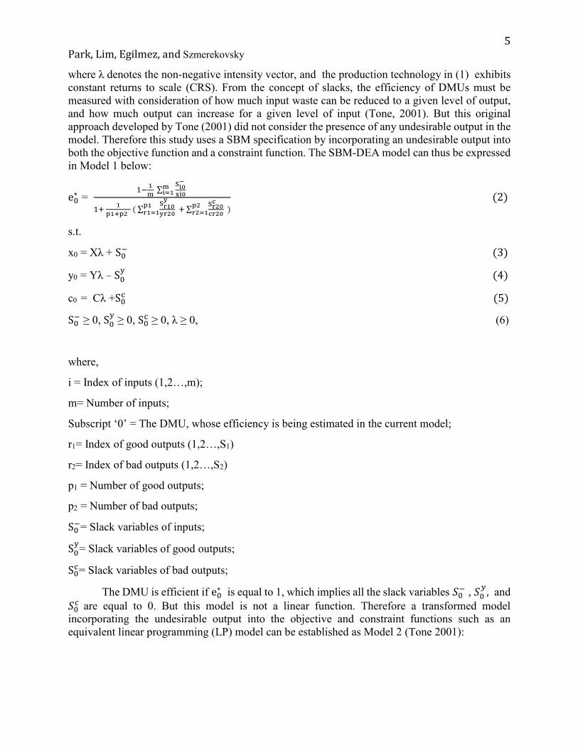
where λ denotes the non-negative intensity vector, and the production technology in (1) exhibits constant returns to scale (CRS). From the concept of slacks, the efficiency of DMUs must be measured with consideration of how much input waste can be reduced to a given level of output, and how much output can increase for a given level of input (Tone, 2001). But this original approach developed by Tone (2001) did not consider the presence of any undesirable output in the model. Therefore this study uses a SBM specification by incorporating an undesirable output into both the objective function and a constraint function. The SBM-DEA model can thus be expressed in Model 1 below:

e0∗ = 1−1

m ∑Si0−

xi0mi=1

1+ 1p1+p2 ( ∑

Sr10y

yr20p1r1=1 + ∑

Sr20c

cr20 p2r2=1 )

(2)

s.t.

x0 = Xλ + S0− (3)

y0 = Yλ - S0y (4)

c0 = Cλ +S0c (5)

S0− ≥ 0, S0y ≥ 0, S0c ≥ 0, λ ≥ 0, (6)

where,

i = Index of inputs (1,2…,m);

m= Number of inputs;

Subscript ‘0’ = The DMU, whose efficiency is being estimated in the current model;

r1= Index of good outputs (1,2…,S1)

r2= Index of bad outputs (1,2…,S2)

p1 = Number of good outputs;

p2 = Number of bad outputs;

S0−= Slack variables of inputs;

S0y= Slack variables of good outputs;

S0c= Slack variables of bad outputs;

The DMU is efficient if e0∗ is equal to 1, which implies all the slack variables 𝑆𝑆0− , 𝑆𝑆0𝑦𝑦, and

𝑆𝑆0𝑐𝑐 are equal to 0. But this model is not a linear function. Therefore a transformed model incorporating the undesirable output into the objective and constraint functions such as an equivalent linear programming (LP) model can be established as Model 2 (Tone 2001):


r0∗ = min t – 1m ∑ Si0

−

xi0mi=1

= t + 1p1+p2

[ ∑ Sr10y

yr20+ ∑ Sr20c

cr20S2r2=1 ]S1

r1=1 (7)

s.t.

x0t = Xß + S0− (8)

y0t = Yß − S0y (9)

c0 t = Cß +S0c (10)

S0− ≥ 0, S0y ≥ 0, S0c ≥ 0, ß ≥ 0, t > 0, (11)

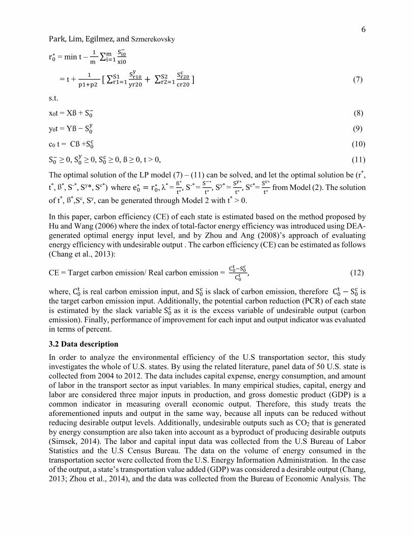
The optimal solution of the LP model (7) – (11) can be solved, and let the optimal solution be (r*, t*, ß*, S-*, Sy*, Sc*) where e0∗ = r0∗, λ* = ß∗

t∗, S-* = S

−∗

t∗, Sy* = S

y∗

t∗, Sc*= S

c∗

t∗ from Model (2). The solution

of t*, ß*,Sc, Sy, can be generated through Model 2 with t* > 0.

In this paper, carbon efficiency (CE) of each state is estimated based on the method proposed by Hu and Wang (2006) where the index of total-factor energy efficiency was introduced using DEA-generated optimal energy input level, and by Zhou and Ang (2008)’s approach of evaluating energy efficiency with undesirable output . The carbon efficiency (CE) can be estimated as follows (Chang et al., 2013):

CE = Target carbon emission/ Real carbon emission = C0t −S0c C0t , (12)

where, C0t is real carbon emission input, and S0c is slack of carbon emission, therefore C0t − S0c is the target carbon emission input. Additionally, the potential carbon reduction (PCR) of each state is estimated by the slack variable S0c as it is the excess variable of undesirable output (carbon emission). Finally, performance of improvement for each input and output indicator was evaluated in terms of percent.

3.2 Data description In order to analyze the environmental efficiency of the U.S transportation sector, this study investigates the whole of U.S. states. By using the related literature, panel data of 50 U.S. state is collected from 2004 to 2012. The data includes capital expense, energy consumption, and amount of labor in the transport sector as input variables. In many empirical studies, capital, energy and labor are considered three major inputs in production, and gross domestic product (GDP) is a common indicator in measuring overall economic output. Therefore, this study treats the aforementioned inputs and output in the same way, because all inputs can be reduced without reducing desirable output levels. Additionally, undesirable outputs such as CO2 that is generated by energy consumption are also taken into account as a byproduct of producing desirable outputs (Simsek, 2014). The labor and capital input data was collected from the U.S Bureau of Labor Statistics and the U.S Census Bureau. The data on the volume of energy consumed in the transportation sector were collected from the U.S. Energy Information Administration. In the case of the output, a state’s transportation value added (GDP) was considered a desirable output (Chang, 2013; Zhou et al., 2014), and the data was collected from the Bureau of Economic Analysis. The


data on CO2 emissions was available from the U.S Energy Information Administration (U.S. EIA). The data descriptions are provided in Table 1.

TABLE 1. Input and output variables and data sources, 2004-2012

Variables Unit Sources

Input Capital expenses

Energy use

Labor

In thousands

Trillion Btu

In thousands (person)

U.S Census Bureau

U.S. Energy Information Administration

U.S Bureau of Labor Statistics

Output Desirable output: Value added (GDP)

Undesirable output: CO2 emission

Million dollars

Million metric tons

Bureau of Economic Analysis

U.S. Energy Information Administration

4. RESULTS AND DISCUSSION

4.1 Input and output indicators

Table 2 shows the descriptive statistics of the state-level data from 2004 to 2012. The capital expenditure of U.S states’ transportation sectors averaged 4.76 billion dollars for 2004 - 2012. The average state transportation sector consumed 599 trillion Btu of energy, employed 167 thousand people, produced 8.09 billion dollars in GDP (value-added) and emitted 38 million metric tons of CO2. There is a much larger difference in capital expenditure, energy input, and GDP across the states as can be seen from the standard deviations in Table 2. On the other hand, relatively small differences can be found in labor input and CO2 emissions. The correlation matrix of inputs and outputs in Table 3 are analyzed to see if there is a significant relationship between the input and output variables. From the results in Table 3, we can see a significantly high correlation exists between the input and the output variables in that the correlation coefficients are all above 0.600.

TABLE 2. Descriptive statistics of input and output, 2004- 2012

Variable N Minimum Maximum Mean Std. Dev Capital 450 3,812.00 30,312,557.00 4,762,591.61 5,301,744.99 Energy 450 19.60 3387.30 599.48 697.83 Labor 450 7.00 951.00 167.65 178.55 GDP (value- added) 450 298.00 53443.00 8,090.03 8982.55 CO2 450 1.07 238.14 37.94 41.57


TABLE 3. Correlation matrix of inputs and outputs

Capital Energy Labor CO2 GDP Capital Pearson Correlation 1 .674** .842** .808** .832**

Sig. (2-tailed) .000 .000 .000 .000 N 450 450 450 450 450

Energy Pearson Correlation .677** 1 .801** .835** .808** Sig. (2-tailed) .000 .000 .000 .000 N 450 450 450 450 450

Labor Pearson Correlation .842** .804** 1 .962** .970** Sig. (2-tailed) .000 .000 .000 .000 N 450 450 450 450 450

CO2 Pearson Correlation .808** .835** .962** 1 .964** Sig. (2-tailed) .000 .000 .000 .000 N 450 450 450 450 450

GDP Pearson Correlation .832** .808** .970** .964** 1 Sig. (2-tailed) .000 .000 .000 .000 N 450 450 450 450 450

**. Correlation is significant at the 0.01 level (2-tailed).

4.2 U.S. States’ environmental efficiency performance

As mentioned in Section 3, the environmental efficiency (EE) score in the transportation sector is evaluated by the e0∗ , because it includes the slack variable of all input and output variables. Then, the carbon efficiency (CE) score is estimated by equation (12), and finally potential carbon reduction (PCR) is calculated by the slack variable 𝑠𝑠0𝑐𝑐. Tables 4 and 5 show the results of EE and CE indicators for each U.S state from 2004 to 2012. The overall average EE performance from 2004 to 2012 of the transportation sector in the U.S indicates that only four states of fifty (Alaska, Illinois, Nebraska and Vermont) were found to be (relatively) environmentally efficient as scores of EE in the four states are 1. In terms of CE, five states (the four states previously mentioned and texas) were found to be (relatively) carbon efficient states. The EE scores for inefficient states ranged from 0.341 to 0.965 (average = 0.640), with Texas ranking first and Alabama ranking last among the inefficient states. CE scores for inefficient states ranged from 0.307 to 0.975 (average = 0.638) with Rhode Island ranking first and South Carolina ranking last among the inefficient states. The ranking is consistent between EE and CE scores over the states. The results of the SBM model indicated that, after accounting for output, input and pollutant slacks, approximately 40% of the states have an above-average EE and CE score suggesting that most of the states’ transportation sectors were not environmentally efficient during the 9-year study period, as states use massive amounts of input resources in order to produce more outputs. Therefore, there is great potential to improve the EE and CE score in each state. The states on the average could accomplish a 36% improvement in EE and 36.2% in CE if all states operate at the frontier of production technology. In addition, there was no significant change in the EE and CE scores from 2004 to 2012. This empirical result might be attributed to the fact that there was no significant growth in carbon emission. But there was a slight decrease in carbon emissions from 2005 to 2008, followed by an increase thereafter. The average EE and CE have the


same trend as the rate of CO2 emissions in the U.S transportation sector (EPA, 2013). In a future study, the most recent data should be added to further analyze the efficiency of states.

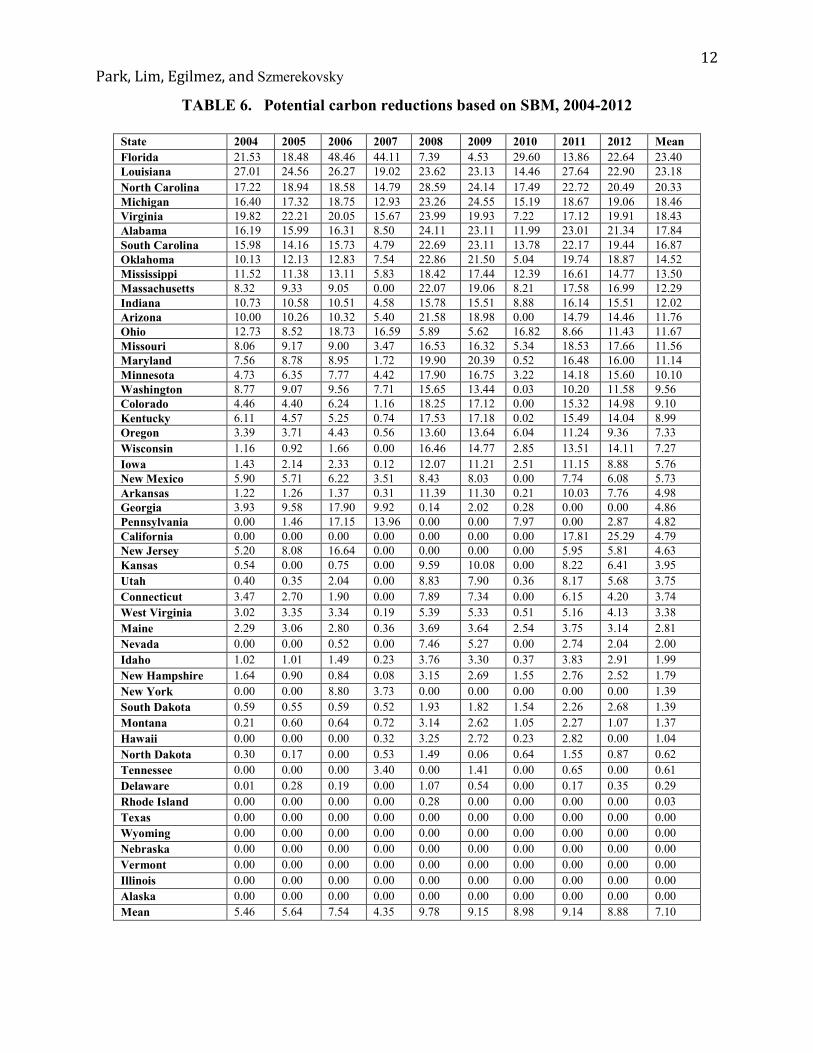
As the results of EE and CE indicate, most of the states are not performing efficiently in the transportation sector, leading to conclusion that there is great potential to reduce carbon emissions in each state, which is also a necessity. We can see in Table 6 that the U.S. transportation sector can reduce a great deal of carbon emissions ranging from at least 0.03 million metric tons to 23.40 million metric tons. The average PCR was found to be 7.10 million metric tons. As shown in the last column of Table 6, on average, 46 U.S. states’ transportation sectors showed excessive CO2 emissions that need to be reduced. Among the states, Florida shows the highest potential for carbon reduction with 23.40 million metric tons followed by Louisiana with 23.18 million metric tons and North Carolina with 20.33 million metric tons. Compared to Louisiana and North Carolina; Florida had a relatively higher EE score but larger PCR. This suggests that the inefficiency in Florida’s transportation can be explained in large part by the presence of environmental impact slack. On the other hand, North Dakota, Tennessee, Delaware and Rhode Island were found to have only a small amount of excess CO2 emissions, showing 0.62, 0.61, 0.29 and 0.03 million metric tons of PCR, respectively.

In spite of that, there are only four environmentally efficient states and most EE scores are quite low. Therefore, it is imperative for us to examine the slack values of inputs and outputs in the model. The purpose of measuring the relative efficiency is to determine the amount of excess inputs and the shortfall of output so that the DMUs can identify the best management practices for sustainable transportation. The estimated slack values and the associated improvements are presented in the parentheses in Table 7. Combining Tables 4,5,6, and 7, it was found that low-ranked environmentally inefficient states have extremely high slack values and high slack percentage in input variables. This pattern suggests that the input levels need to be lowered by the suggested amount in order to achieve 100% efficiency. For example, among the environmentally inefficient states, Alabama has a higher excess in the input variables, including capital, energy, labor, and CO2, while producing insufficient goods and services (GDP) related to the transportation sector. Other problematic states such as Maryland, Mississippi, Colorado and South Carolina, also show much waste in input variables and have high shortfalls in GDP as well. In addition, the third-best state among the inefficient states, California, has extremely high excess values in capital, energy, and labor, as well as a shortfall in GDP. Florida and Louisiana show the greatest excess in undesirable output (CO2). The percentage of excess of inputs shows that, on average, capital investment has the highest percentage slack at 31.3%, CO2 has the second highest in slack at 21.9%, and labor has the third highest in slack at 14%, while energy input has relatively less slack at 2.4%. The results indicate that the federal government and state agencies should focus on capital investment that state policymakers can reduce unnecessary investment in the transportation system, and force more efficient use of labor in the transportation sector in order to improve environmental efficiency.


TABLE 4. Environmental efficiency based on SBM, 2004-2012

State 2004 2005 2006 2007 2008 2009 2010 2011 2012 Mean Alaska 1.000 1.000 1.000 1.000 1.000 1.000 1.000 1.000 1.000 1.000 Illinois 1.000 1.000 1.000 1.000 1.000 1.000 1.000 1.000 1.000 1.000 Nebraska 1.000 1.000 1.000 1.000 1.000 1.000 1.000 1.000 1.000 1.000 Vermont 1.000 1.000 1.000 1.000 1.000 1.000 1.000 1.000 1.000 1.000 Texas 1.000 1.000 1.000 0.686 1.000 1.000 1.000 1.000 1.000 0.965 Wyoming 0.838 0.984 1.000 0.818 1.000 1.000 1.000 1.000 1.000 0.960 California 1.000 1.000 1.000 1.000 1.000 1.000 1.000 0.825 0.776 0.956 Hawaii 1.000 1.000 1.000 0.758 0.748 0.820 0.911 0.842 1.000 0.898 Rhode Island 0.797 0.841 0.851 0.868 0.844 1.000 0.873 1.000 1.000 0.897 New Jersey 0.832 0.861 0.779 1.000 1.000 1.000 0.832 0.771 0.790 0.874 Tennessee 1.000 1.000 1.000 0.302 1.000 0.896 0.720 0.854 1.000 0.864 Delaware 0.747 0.734 0.789 1.000 0.719 0.764 1.000 0.879 0.834 0.830 Georgia 0.869 0.774 0.677 0.708 0.846 0.890 0.676 1.000 1.000 0.827 North Dakota 0.737 0.813 1.000 0.713 0.812 0.917 0.811 0.849 0.745 0.822 New York 0.739 0.791 0.726 0.666 0.820 0.831 1.000 0.813 0.799 0.798 Montana 0.683 0.728 0.709 0.644 0.672 0.740 0.747 0.742 0.712 0.709 South Dakota 0.700 0.711 0.746 0.659 0.672 0.684 0.700 0.662 0.626 0.684 Ohio 0.650 0.713 0.652 0.527 0.742 0.742 0.781 0.661 0.662 0.681 Pennsylvania 0.760 0.703 0.627 0.548 0.699 0.695 0.683 0.656 0.650 0.669 Florida 0.620 0.653 0.600 0.554 0.708 0.747 0.613 0.706 0.669 0.652 New Hampshire 0.645 0.715 0.680 0.580 0.588 0.618 0.595 0.674 0.695 0.643 Idaho 0.574 0.596 0.596 0.593 0.547 0.577 0.691 0.579 0.602 0.595 Maine 0.529 0.538 0.567 0.519 0.577 0.605 0.743 0.598 0.595 0.586 Virginia 0.520 0.504 0.535 1.000 0.500 0.585 0.514 0.526 0.534 0.580 Indiana 0.582 0.609 0.595 0.623 0.553 0.561 0.513 0.550 0.569 0.573 Nevada 0.565 0.568 0.531 0.501 0.554 0.597 0.553 0.642 0.631 0.571 Connecticut 0.506 0.535 0.530 0.619 0.571 0.580 0.588 0.592 0.579 0.567 Arkansas 0.538 0.572 0.580 0.624 0.519 0.525 0.569 0.535 0.561 0.558 Washington 0.575 0.591 0.547 0.465 0.516 0.557 0.569 0.578 0.587 0.554 Kentucky 0.583 0.672 0.544 0.677 0.436 0.509 0.504 0.500 0.516 0.549 New Mexico 0.475 0.453 0.444 0.410 0.467 0.482 1.000 0.569 0.547 0.539 Kansas 0.502 0.526 0.517 0.601 0.505 0.520 0.558 0.548 0.569 0.538 Missouri 0.568 0.589 0.555 0.459 0.558 0.550 0.545 0.468 0.505 0.533 Utah 0.565 0.602 0.549 0.528 0.492 0.513 0.497 0.499 0.492 0.526 Louisiana 0.454 0.432 0.469 0.603 0.553 0.569 0.507 0.470 0.541 0.511 Michigan 0.568 0.549 0.496 0.432 0.486 0.463 0.453 0.526 0.553 0.503 Minnesota 0.582 0.567 0.467 0.591 0.438 0.438 0.424 0.461 0.461 0.492 West Virginia 0.458 0.462 0.480 0.431 0.478 0.486 0.558 0.517 0.495 0.485 Arizona 0.459 0.516 0.466 0.581 0.367 0.410 0.469 0.483 0.503 0.473 Iowa 0.487 0.464 0.459 0.542 0.441 0.451 0.471 0.452 0.453 0.469 Massachusetts 0.405 0.404 0.388 1.000 0.367 0.403 0.405 0.412 0.429 0.468 Wisconsin 0.540 0.540 0.493 0.449 0.395 0.436 0.422 0.415 0.427 0.457 North Carolina 0.479 0.487 0.454 0.391 0.429 0.483 0.383 0.430 0.466 0.445 Oregon 0.491 0.472 0.449 0.417 0.423 0.421 0.357 0.445 0.474 0.439 Oklahoma 0.454 0.452 0.436 0.353 0.353 0.368 0.596 0.408 0.410 0.426 Maryland 0.427 0.416 0.386 0.484 0.356 0.375 0.408 0.396 0.365 0.402 Mississippi 0.359 0.399 0.349 0.339 0.334 0.387 0.405 0.373 0.367 0.368 Colorado 0.347 0.396 0.368 0.418 0.340 0.351 0.337 0.342 0.389 0.365 South Carolina 0.317 0.337 0.343 0.434 0.342 0.375 0.364 0.337 0.347 0.355 Alabama 0.340 0.338 0.336 0.357 0.329 0.329 0.354 0.337 0.344 0.341 Mean 0.637 0.652 0.635 0.629 0.622 0.645 0.654 0.638 0.645 0.640


TABLE 5. Carbon efficiency based on SBM, 2004-2012

State 2004 2005 2006 2007 2008 2009 2010 2011 2012 Mean Alaska 1.000 1.000 1.000 1.000 1.000 1.000 1.000 1.000 1.000 1.000 Nebraska 1.000 1.000 1.000 1.000 1.000 1.000 1.000 1.000 1.000 1.000 Illinois 1.000 1.000 1.000 1.000 1.000 1.000 1.000 1.000 1.000 1.000 Vermont 1.000 1.000 1.000 1.000 1.000 1.000 1.000 1.000 1.000 1.000 Texas 1.000 1.000 1.000 1.000 1.000 1.000 1.000 1.000 1.000 1.000 Rhode Island 0.942 0.955 0.950 1.000 0.932 1.000 1.000 1.000 1.000 0.975 California 1.000 1.000 1.000 1.000 1.000 1.000 1.000 0.913 0.856 0.974 Wyoming 0.767 0.980 1.000 1.000 1.000 1.000 1.000 1.000 1.000 0.972 Tennessee 1.000 1.000 1.000 0.735 1.000 0.871 0.777 0.870 1.000 0.917 New York 0.852 0.967 0.838 0.929 0.895 0.924 1.000 0.931 0.872 0.912 Delaware 0.860 0.822 0.832 1.000 0.787 0.831 1.000 0.915 0.903 0.883 Hawaii 1.000 1.000 1.000 0.916 0.665 0.705 0.929 0.724 1.000 0.882 New Jersey 0.714 0.783 0.619 1.000 1.000 1.000 0.835 0.806 0.833 0.843 North Dakota 0.731 0.781 1.000 0.926 0.754 0.893 0.908 0.765 0.758 0.835 Georgia 0.774 0.772 0.587 0.792 0.716 0.902 0.736 1.000 1.000 0.809 Pennsylvania 0.713 0.769 0.650 0.692 0.703 0.720 0.794 0.704 0.701 0.716 South Dakota 0.734 0.737 0.737 0.842 0.682 0.673 0.741 0.629 0.599 0.708 Montana 0.665 0.638 0.634 0.691 0.623 0.666 0.857 0.671 0.736 0.687 Ohio 0.600 0.774 0.615 0.645 0.643 0.641 0.716 0.582 0.600 0.646 Nevada 0.561 0.550 0.516 0.537 0.544 0.636 0.794 0.791 0.835 0.640 New Hampshire 0.599 0.657 0.668 0.754 0.567 0.584 0.668 0.586 0.611 0.633 Idaho 0.601 0.609 0.580 0.822 0.572 0.588 0.684 0.564 0.587 0.623 Florida 0.562 0.637 0.564 0.614 0.643 0.674 0.687 0.586 0.570 0.615 Indiana 0.512 0.637 0.507 0.726 0.495 0.502 0.543 0.573 0.582 0.564 Maine 0.547 0.510 0.524 0.638 0.550 0.541 0.655 0.533 0.565 0.563 Washington 0.535 0.570 0.510 0.495 0.498 0.536 0.629 0.573 0.565 0.546 Connecticut 0.441 0.463 0.485 0.538 0.530 0.544 0.608 0.607 0.668 0.543 Kansas 0.512 0.537 0.506 0.514 0.497 0.485 0.593 0.567 0.637 0.539 Arkansas 0.493 0.492 0.487 0.821 0.445 0.439 0.547 0.502 0.561 0.532 Utah 0.523 0.527 0.479 0.519 0.482 0.510 0.593 0.528 0.596 0.529 Wisconsin 0.588 0.615 0.543 0.522 0.437 0.471 0.525 0.515 0.498 0.524 West Virginia 0.471 0.467 0.472 0.536 0.512 0.508 0.646 0.530 0.531 0.519 Missouri 0.525 0.610 0.493 0.490 0.478 0.486 0.501 0.455 0.511 0.506 Michigan 0.511 0.621 0.441 0.464 0.426 0.411 0.486 0.560 0.556 0.497 Kentucky 0.488 0.590 0.472 0.453 0.427 0.440 0.510 0.510 0.506 0.488 Minnesota 0.552 0.539 0.442 0.466 0.434 0.446 0.503 0.508 0.482 0.486 Iowa 0.488 0.472 0.465 0.470 0.440 0.465 0.527 0.486 0.554 0.485 Colorado 0.449 0.482 0.400 0.781 0.395 0.416 0.482 0.470 0.479 0.484 New Mexico 0.382 0.393 0.384 0.442 0.409 0.409 1.000 0.443 0.461 0.480 Virginia 0.431 0.482 0.430 0.425 0.422 0.471 0.592 0.491 0.557 0.478 Arizona 0.405 0.442 0.406 0.706 0.372 0.408 0.515 0.496 0.498 0.472 Oregon 0.446 0.440 0.425 0.423 0.403 0.399 0.476 0.467 0.524 0.445 North Carolina 0.454 0.535 0.417 0.404 0.373 0.412 0.510 0.425 0.453 0.442 Massachusetts 0.405 0.382 0.366 0.370 0.340 0.380 0.444 0.432 0.449 0.396 Maryland 0.388 0.371 0.365 0.370 0.351 0.357 0.450 0.437 0.465 0.395 Louisiana 0.280 0.312 0.297 0.367 0.409 0.485 0.490 0.420 0.469 0.392 Oklahoma 0.342 0.320 0.312 0.530 0.293 0.304 0.421 0.382 0.416 0.369 Alabama 0.283 0.285 0.283 0.524 0.282 0.289 0.347 0.316 0.344 0.328 Mississippi 0.303 0.305 0.286 0.310 0.282 0.297 0.383 0.327 0.338 0.315 South Carolina 0.270 0.289 0.275 0.501 0.260 0.256 0.325 0.283 0.307 0.307 Mean 0.614 0.642 0.605 0.674 0.599 0.620 0.689 0.638 0.661 0.638


TABLE 6. Potential carbon reductions based on SBM, 2004-2012

State 2004 2005 2006 2007 2008 2009 2010 2011 2012 Mean Florida 21.53 18.48 48.46 44.11 7.39 4.53 29.60 13.86 22.64 23.40 Louisiana 27.01 24.56 26.27 19.02 23.62 23.13 14.46 27.64 22.90 23.18 North Carolina 17.22 18.94 18.58 14.79 28.59 24.14 17.49 22.72 20.49 20.33 Michigan 16.40 17.32 18.75 12.93 23.26 24.55 15.19 18.67 19.06 18.46 Virginia 19.82 22.21 20.05 15.67 23.99 19.93 7.22 17.12 19.91 18.43 Alabama 16.19 15.99 16.31 8.50 24.11 23.11 11.99 23.01 21.34 17.84 South Carolina 15.98 14.16 15.73 4.79 22.69 23.11 13.78 22.17 19.44 16.87 Oklahoma 10.13 12.13 12.83 7.54 22.86 21.50 5.04 19.74 18.87 14.52 Mississippi 11.52 11.38 13.11 5.83 18.42 17.44 12.39 16.61 14.77 13.50 Massachusetts 8.32 9.33 9.05 0.00 22.07 19.06 8.21 17.58 16.99 12.29 Indiana 10.73 10.58 10.51 4.58 15.78 15.51 8.88 16.14 15.51 12.02 Arizona 10.00 10.26 10.32 5.40 21.58 18.98 0.00 14.79 14.46 11.76 Ohio 12.73 8.52 18.73 16.59 5.89 5.62 16.82 8.66 11.43 11.67 Missouri 8.06 9.17 9.00 3.47 16.53 16.32 5.34 18.53 17.66 11.56 Maryland 7.56 8.78 8.95 1.72 19.90 20.39 0.52 16.48 16.00 11.14 Minnesota 4.73 6.35 7.77 4.42 17.90 16.75 3.22 14.18 15.60 10.10 Washington 8.77 9.07 9.56 7.71 15.65 13.44 0.03 10.20 11.58 9.56 Colorado 4.46 4.40 6.24 1.16 18.25 17.12 0.00 15.32 14.98 9.10 Kentucky 6.11 4.57 5.25 0.74 17.53 17.18 0.02 15.49 14.04 8.99 Oregon 3.39 3.71 4.43 0.56 13.60 13.64 6.04 11.24 9.36 7.33 Wisconsin 1.16 0.92 1.66 0.00 16.46 14.77 2.85 13.51 14.11 7.27 Iowa 1.43 2.14 2.33 0.12 12.07 11.21 2.51 11.15 8.88 5.76 New Mexico 5.90 5.71 6.22 3.51 8.43 8.03 0.00 7.74 6.08 5.73 Arkansas 1.22 1.26 1.37 0.31 11.39 11.30 0.21 10.03 7.76 4.98 Georgia 3.93 9.58 17.90 9.92 0.14 2.02 0.28 0.00 0.00 4.86 Pennsylvania 0.00 1.46 17.15 13.96 0.00 0.00 7.97 0.00 2.87 4.82 California 0.00 0.00 0.00 0.00 0.00 0.00 0.00 17.81 25.29 4.79 New Jersey 5.20 8.08 16.64 0.00 0.00 0.00 0.00 5.95 5.81 4.63 Kansas 0.54 0.00 0.75 0.00 9.59 10.08 0.00 8.22 6.41 3.95 Utah 0.40 0.35 2.04 0.00 8.83 7.90 0.36 8.17 5.68 3.75 Connecticut 3.47 2.70 1.90 0.00 7.89 7.34 0.00 6.15 4.20 3.74 West Virginia 3.02 3.35 3.34 0.19 5.39 5.33 0.51 5.16 4.13 3.38 Maine 2.29 3.06 2.80 0.36 3.69 3.64 2.54 3.75 3.14 2.81 Nevada 0.00 0.00 0.52 0.00 7.46 5.27 0.00 2.74 2.04 2.00 Idaho 1.02 1.01 1.49 0.23 3.76 3.30 0.37 3.83 2.91 1.99 New Hampshire 1.64 0.90 0.84 0.08 3.15 2.69 1.55 2.76 2.52 1.79 New York 0.00 0.00 8.80 3.73 0.00 0.00 0.00 0.00 0.00 1.39 South Dakota 0.59 0.55 0.59 0.52 1.93 1.82 1.54 2.26 2.68 1.39 Montana 0.21 0.60 0.64 0.72 3.14 2.62 1.05 2.27 1.07 1.37 Hawaii 0.00 0.00 0.00 0.32 3.25 2.72 0.23 2.82 0.00 1.04 North Dakota 0.30 0.17 0.00 0.53 1.49 0.06 0.64 1.55 0.87 0.62 Tennessee 0.00 0.00 0.00 3.40 0.00 1.41 0.00 0.65 0.00 0.61 Delaware 0.01 0.28 0.19 0.00 1.07 0.54 0.00 0.17 0.35 0.29 Rhode Island 0.00 0.00 0.00 0.00 0.28 0.00 0.00 0.00 0.00 0.03 Texas 0.00 0.00 0.00 0.00 0.00 0.00 0.00 0.00 0.00 0.00 Wyoming 0.00 0.00 0.00 0.00 0.00 0.00 0.00 0.00 0.00 0.00 Nebraska 0.00 0.00 0.00 0.00 0.00 0.00 0.00 0.00 0.00 0.00 Vermont 0.00 0.00 0.00 0.00 0.00 0.00 0.00 0.00 0.00 0.00 Illinois 0.00 0.00 0.00 0.00 0.00 0.00 0.00 0.00 0.00 0.00 Alaska 0.00 0.00 0.00 0.00 0.00 0.00 0.00 0.00 0.00 0.00 Mean 5.46 5.64 7.54 4.35 9.78 9.15 8.98 9.14 8.88 7.10


TABLE 7. Summary of average excess in inputs and shortfall in outputs, 2004-2012

State

Inputs (Excess) Undesirable Output (Excess)

Desirable Output (Shortfall)

Capital ($)

Slack (%)

Energy (Btu)

Slack (%)

labor (Person)

Slack (%)

CO2 (Ton)

Slack (%)

GDP ($)

Slack (%)

Alabama 960010.8 (-21.3) 1.6 (0.0) 30.5 (-14.4) 17.8 (-52.0) 2107.9 (32.9) Alaska 0.0 (0.0) 0.0 (0.0) 0.0 (0.0) 0.0 (0.0) 0.0 (0.0) Arizona 2002066.5 (-43.2) 9.5 (-1.7) 24.3 (-14.3) 11.8 (-33.8) 209.6 (1.2) Arkansas 664862.4 (-24.5) 0.3 (-0.1) 22.7 (-19.5) 5.0 (-24.4) 51.9 (0.8) California 9333921.1 (0.0) 25.3 (0.0) 144.0 (0.0) 4.8 (-2.2) 2134.7 (0.0) Colorado 1894182.3 (-46.8) 2740.2 (-86.5) 16.4 (-13.3) 9.1 (-30.5) 62.3 (0.5) Connecticut 995853.6 (-38.7) 6.7 (-3.3) 16.3 (-25.3) 3.7 (-21.9) 63.8 (0.5) Delaware 668498.0 (-20.9) 0.7 (-0.4) 6.9 (-9.5) 0.3 (-6.0) 86.3 (3.0) Florida 8996813.9 (-29.2) 6.1 (-0.3) 119.9 (-4.1) 23.4 (-21.6) 1438.4 (3.9) Georgia 1679037.6 (-11.1) 1.1 (0.0) 73.6 (-3.3) 4.9 (-7.4) 77.3 (0.0) Hawaii 103764.6 (0.0) 0.0 (0.0) 0.0 (0.0) 1.0 (-9.2) 0.0 (0.0) Idaho 656505.5 (-34.7) 0.6 (-0.8) 14.2 (-32.1) 2.0 (-22.0) 301.9 (27.7) Illinois 4432319.3 (0.0) 6.0 (0.0) 110.8 (0.0) 0.0 (0.0) 0.0 (0.0) Indiana 1393073.0 (-28.4) 4.0 (-0.3) 67.9 (-26.2) 12.0 (-27.5) 315.7 (4.0) Iowa 1714996.1 (-48.7) 2.0 (-0.7) 45.4 (-40.1) 5.8 (-26.9) 162.9 (6.0) Kansas 1602683.8 (-50.0) 3.2 (-1.8) 12.5 (-18.6) 4.0 (-20.7) 0.0 (0.4) Kentucky 1636427.3 (-36.2) 2.2 (-0.3) 30.6 (-15.8) 9.0 (-27.1) 95.4 (2.7) Louisiana 554242.0 (0.0) 0.2 (0.0) 2.3 (0.0) 23.2 (-46.2) 791.9 (0.0) Maine 648567.3 (-28.0) 0.5 (-0.5) 11.3 (-22.3) 2.8 (-32.3) 406.1 (50.3) Maryland 3132041.5 (-56.9) 8.7 (-2.1) 19.9 (-16.4) 11.1 (-36.0) 255.8 (2.3) Massachusetts 2618724.1 (-52.4) 8.9 (-1.9) 28.5 (-16.9) 12.3 (-38.1) 246.3 (3.2) Michigan 2491423.2 (-38.4) 15.8 (-1.9) 75.8 (-24.8) 18.5 (-35.2) 534.6 (4.7) Minnesota 3663932.0 (-59.2) 9.5 (-2.0) 24.6 (-12.3) 10.1 (-29.3) 69.0 (0.4) Mississippi 1002122.2 (-31.7) 2.2 (-0.5) 10.7 (-13.2) 13.5 (-52.7) 1337.2 (37.5) Missouri 1949786.2 (-37.2) 2.5 (-0.2) 44.5 (-21.6) 11.6 (-28.4) 456.3 (7.4) Montana 1145352.6 (-43.4) 0.9 (-0.7) 1.5 (-4.9) 1.4 (-16.5) 79.5 (16.7) Nebraska 0.0 (0.0) 0.0 (0.0) 0.0 (0.0) 0.0 (0.0) 0.0 (0.0) Nevada 4848524.0 (-60.1) 1.3 (-0.8) 14.7 (-23.3) 2.0 (-12.7) 0.0 (0.3) New Hampshire 920129.6 (-32.3) 0.9 (-0.8) 7.7 (-16.3) 1.8 (-24.6) 188.8 (39.2) New Jersey 1286622.8 (-8.5) 3.4 (0.0) 33.6 (-0.5) 4.6 (-7.0) 8.7 (0.0) New Mexico 630779.4 (-25.9) 2.2 (-0.9) 6.3 (-16.5) 5.7 (-38.8) 755.6 (39.2) New York 10321008.7 (-45.6) 20.4 (-0.5) 175.5 (-20.6) 1.4 (-1.9) 0.0 (0.0) North Carolina 4344011.3 (-44.0) 5.6 (-0.6) 82.3 (-21.0) 20.3 (-39.8) 1038.6 (9.9) North Dakota 1249116.5 (-31.2) 3.2 (-2.0) 1.0 (-1.4) 0.6 (-8.9) 95.8 (8.8) Ohio 2854580.2 (-31.9) 8.1 (-0.5) 138.8 (-26.5) 11.7 (-17.0) 62.4 (2.1) Oklahoma 761736.8 (-22.9) 3.5 (-0.8) 5.4 (-8.7) 14.5 (-46.1) 559.4 (6.8) Oregon 2970890.4 (-50.9) 2.1 (-0.6) 24.5 (-23.3) 7.3 (-32.2) 141.9 (2.4) Pennsylvania 6901247.5 (-54.7) 9.8 (-0.4) 159.6 (-27.2) 4.8 (-7.0) 0.0 (1.0) Rhode Island 765612.9 (-17.3) 1.9 (-0.3) 11.5 (-20.2) 0.0 (-0.7) 68.1 (0.0) South Carolina 813063.1 (-19.7) 1.1 (-0.1) 23.2 (-6.9) 16.9 (-53.9) 1602.3 (42.8) South Dakota 1128334.9 (-47.3) 1.4 (-1.4) 2.5 (-5.0) 1.4 (-21.9) 179.0 (34.0) Tennessee 943627.2 (-19.0) 1.1 (-0.2) 18.3 (-1.5) 0.6 (-1.4) 0.0 (0.0) Texas 5494902.7 (0.0) 8.8 (0.0) 74.1 (0.0) 0.0 (0.0) 882.7 (0.0) Utah 1542717.3 (-48.8) 0.9 (-0.6) 18.8 (-24.7) 3.7 (-21.8) 106.7 (3.2) Vermont 878603.2 (0.0) 0.4 (0.0) 4.4 (0.0) 0.0 (0.0) 149.8 (0.0) Virginia 2891505.3 (-43.3) 6.8 (-0.7) 24.4 (-9.1) 18.4 (-34.7) 758.3 (3.3) Washington 4156807.1 (-55.9) 1.7 (-0.1) 43.4 (-11.0) 9.6 (-22.1) 168.1 (3.3) West Virginia 1274187.0 (-52.8) 4.9 (-3.3) 15.4 (-32.8) 3.4 (-28.4) 251.7 (29.2) Wisconsin 3656673.2 (-62.2) 3.0 (-1.1) 78.0 (-37.0) 7.3 (-24.1) 0.0 (0.0) Wyoming 329295.6 (-11.3) 2.1 (-0.2) 1.1 (0.0) 0.0 (0.0) 0.0 (0.0) Mean 2338103.7 (-31.3) 59.1 (-2.4) 38.4 (-14.0) 7.1 (-21.9) 366.1 (8.6) Note: Slack (% ) = (Target-Actual) / Actual × 100


5. CONCLUSION

Sustainable development in U.S. transportation is essential for economic growth and mobility, but also for the environment. However, no study has been conducted on the environmental efficiency of the U.S. transportation sector. This study uses a non-radial SBM-DEA model with an undesirable output (CO2) to measure the environmental efficiency of the U.S transportation sector from 2004 to 2012. Using the SBM-DEA model, environmental efficiency (EE), carbon efficiency (CE) and potential carbon reduction (PCR) are calculated for each state, and we measure the size of slack input resources and excess CO2 emissions as well as the shortfall of desirable output (GDP). According to the results we draw the following conclusions: 1) Most states had an average EE below 0.64 during 2004-2012, meaning that these states had considerable room for improvements in transportation environmental efficiency; 2) among the 50 U.S states, four states were found to be environmentally efficient (Alaska, Illinois, Nebraska and Vermont), the remaining 46 were inefficient with Alabama, South Carolina, Colorado and Mississippi being the most inefficient with average EE and CE scores below 0.4; 3) during the 2004-2012 study period, the trend of EE and CE slightly decreased between 2005 and 2008 and then began to increase; this is consistent with the rate of CO2 emissions in the U.S transportation sector during the same time period; 4) there was a large PCR for most of U.S states; the average PCR was found to be 7.10 million metric tons; 5) the slack analysis showed that most states had high excess in capital expenses, labor use, and CO2, and shortfall in GDP. The findings provide policy insights as well as an overview of U.S. transportation sector’s environmental performance towards the development of a sustainable transportation industry in the U.S. First of all, the slack analysis shows the potential improvement of states’ environmental efficiency performances in the transportation sector through reducing input and environmental slacks. Second, the policy should adopt the goal and strategy of encouraging energy conservation to reduce CO2 emissions in the transportation sector. The DEA benchmarking results of this study show that state policymakers could learn and adopt the best practices in eco-efficient states to enhance transportation environmental efficiency. Finally, the U.S could improve technological innovation and the current fuel economy standards to produce a more environmentally efficient transportation system. Although this study provided an overall understanding of environmental performance of the U.S. transportation sector, limitations exist, which can be further investigated. First of all, individual states’ performances were compared with other states in the country, and the results may be sensitive to the number of inputs and outputs as well as the levels of aggregation in the data. Also, this study used GDP as the only good output, but different states have different ways of generating GDP and in many cases serve as complements to each other. Therefore, a potential for future research would be to break GDP (or some other indicator) down by market segment to try to capture the relative efficiencies of the states doing different things to generate GDP. Furthermore, the panel data over the years for multiple DMUs can also be analyzed using stochastic frontier analysis to compare the eco-efficiency scores. Lastly, more up-to-date data should be collected in the future to analyze current changes in environmental efficiency in the U.S transportation sector.

References


Banker, R., Charnes, A., & Cooper, W. (1984). Some models for estimating technical and scale inefficiencies in data envelopment analysis. Management Science, 30(9), 1078–1092.

Barba-Gutiérrez, Y. (2009). Eco-efficiency of electric and electronic appliances: a data envelopment analysis (DEA). Environmental Modeling & Assessment, 14(4), 439–447. Retrieved from http://link.springer.com/article/10.1007/s10666-007-9134-2

Benjaafar, S., & Savelsbergh, M. (2014). Carbon-aware transport and logistics. EURO Journal on Transportation and Logistics, 3(1), 1–3.

Caves, D., Christensen, L., & Diewert, W. (1982). Multilateral comparisons of output, input, and productivity using superlative index numbers. The Economic Journal, 73–86.

Chang, Y.-T. (2013). Environmental efficiency of ports: a data envelopment analysis approach. Maritime Policy & Management, 40(5), 467–478. http://doi.org/10.1080/03088839.2013.797119

Chang Y.-T., Zhang, N., Danao, D., & Zhang, N. (2013). Environmental efficiency analysis of transportation system in China: A non-radial DEA approach. Energy Policy 58: 277-283.

Charnes, A., Cooper, W., & Rhodes, E. (1978). Measuring the efficiency of decision making units. European Journal of Operational Research, 2(6), 429–444.

Charnes, A., Haag, S., Jaska, P. & Semple, J. (1992). Sensitivity of efficiency classifications in the additive model of data envelopment analysis. International Journal of Systems Science, 23(5), 789–798. http://doi.org/10.1080/00207729208949248

Charnes, A., Rousseau, J. J., & Semple, J. H. (1996). Sensitivity and stability of efficiency classifications in Data Envelopment Analysis. Journal of Productivity Analysis, 7(1), 5–18. http://doi.org/10.1007/BF00158473

Choi, J., Park, Y.S., & Park, J.D. (2015). Development of an Aggregate Air Quality Index Using a PCA-based Method: A Case Study of the US Transportation Sector. American Journal of Industrial and Business Management, 5(02),53

Cook,W.,& Seiford,L.(2009). Data envelopment analysis (DEA)-Thirty years on. European Journal of Operational Research, 192(1), 1-17.

Cooper, W., Seiford, L., & Tone, K. (2007). Data envelopment analysis: a comprehensive text with models, applications, references and DEA-solver software. Springer Science & Business Media.

Cullinane, K., & Song, D. (2006). Estimating the relative efficiency of European container ports: a stochastic frontier analysis. Research in Transportation Economics, 16, 85–115.


Egilmez, G., & Park, Y. S. (2014). Transportation Related Carbon, Energy and Water Footprint Analysis of U.S. Manufacturing: An Eco-efficiency Assessment. Transportation Research, Part D, 32, 143-159.

Egilmez, G., Kucukvar, M., & Tatari, O. (2013). Sustainability Assessment of US Manufacturing Sectors: An Economic Input Output-based Frontier Approach. Journal of Cleaner Production, 53, 91–102.

EPA, (2013). Greenhouse Gas Emissions: Transportation Sector Emissions.

Färe, R., Grosskopf, S., Lovell, C., & Pasurka, C. (1989). Multilateral productivity comparisons when some outputs are undesirable: a nonparametric approach. The Review of Economics and Statistics, 71(1), 90–98.

Frey, H. C., & Kuo, P. (2007). Assessment of Potential Reduction in Greenhouse Gas ( GHG ) Emissions in Freight Transportation, (c), 1–7.

Goldman, T., & Gorham, R. (2006). Sustainable urban transport: Four innovative directions. Technology in Society, 28(1-2), 261–273. http://doi.org/10.1016/j.techsoc.2005.10.007

Hendrickson, C., Cicas, G., & Matthews, H. (2006). Transportation sector and supply chain performance and sustainability. Transportation Research Record: Journal of the Transportation Research Board, (1983), 151-157.

Hernandez-Sancho,F.(2011). Energy efficiency in Spanish wastewater treatment plants: A non-radial DEA approach. Science of the Total Environment, 409(14), 2693-2699

Hu, J., & Wang, S. (2006). Total-factor energy efficiency of regions in China. Energy Policy, 34(17), 3206–3217.

Leggett, J. A. (2014). President Obama’s Climate Action Plan (pp. 1–2). Retrieved from https://www.whitehouse.gov/sites/default/files/image/president27sclimateactionplan.pdf.

Li, H., Fang, K., Yang, W., Wang, D., & Hong, X. (2013). Regional environmental efficiency evaluation in China: Analysis based on the Super-SBM model with undesirable outputs. Mathematical and Computer Modeling, 58(5), 1018–1031.

Lin, L. C., & Hong, C. H. (2006). Operational performance evaluation of international major airports: An application of data envelopment analysis. Journal of Air Transport Management, 12(6), 342–351. http://doi.org/10.1016/j.jairtraman.2006.08.002

Lovell, C., Pastor, J., & Turner, J. (1995). Measuring macroeconomic performance in the OECD: a comparison of European and non-European countries. European Journal of Operational Research, 87(3), 507–518.

https://www.whitehouse.gov/sites/default/files/image/president27sclimateactionplan.pdf


Lozano, S., & Gutiérrez, E. (2011). Slacks-based measure of efficiency of airports with airplanes delays as undesirable outputs. Computers & Operations Research, 38(1), 131–139.

Merkert, R., & Hensher, D. A. (2011). The impact of strategic management and fleet planning on airline efficiency – A random effects Tobit model based on DEA efficiency scores. Transportation Research Part A: Policy and Practice, 45(7), 686–695. http://doi.org/10.1016/j.tra.2011.04.015

Park, Y.S., Egilmez, G., & Kucukvar, M. (2015). A Novel Life Cycle-based Principle Component Analysis Framework for Eco-efficiency Analysis: Case of the United States Manufacturing and Transportation Nexus.” Journal of Cleaner Production, 92, 327-342

Pittman, R. (1983). Multilateral productivity comparisons with undesirable outputs. The Economic Journal, 883–891.

RITA. (2014). National Transportation Statistics 2014 | Bureau of Transportation Statistics. Retrieved July 11, 2014, from http://www.rita.dot.gov/bts/sites/rita.dot.gov.bts/files/publications/national_transportation_statistics/index.html

Rousseau, J. J., & Semple, J. H. (1995). Radii of Classification Preservation in Data Envelopment Analysis: A Case Study of “Program Follow-Through.” The Journal of the Operational Research Society, 46(8), 943–957.

Scheraga, C. A. (2004). Operational efficiency versus financial mobility in the global airline industry: a data envelopment and Tobit analysis. Transportation Research Part A: Policy and Practice, 38(5), 383–404. http://doi.org/10.1016/j.tra.2003.12.003

Seiford, L. M., & Zhu, J. (2002). Modeling undesirable factors in efficiency evaluation. European Journal of Operational Research, 142(1), 16–20.

Simsek, N. (2014). Energy efficiency with undesirable output at the economy wide level: corss country comparison in OECD sample. American Journal of Energy Research, 2(1), 9-17

Tone, K. (2001). A slacks-based measure of efficiency in data envelopment analysis. European Journal of Operational Research, 130(3), 498–509.

US EPA. (2014). U.S. Greenhouse Gas Inventory Report: 1990-2013. Washington: Environmental Protection Agency. Retrieved from http://www.epa.gov/climatechange/ghgemissions/usinventoryreport.html

Watanabe, M., & Tanaka, K. (2007). Efficiency analysis of Chinese industry: a directional distance function approach. Energy Policy, 35(12), 6323–6331.

WCED. (1987). World Commision on Environment and Development. 1987. Retrieved from www.un-documents.net/our-common-future.pdf


Zhang, B., Bi, J., Fan, Z., Yuan, Z., & Ge, J. (2008). Eco-efficiency analysis of industrial system in China: A data envelopment analysis approach. Ecological Economics, 68(1-2), 306–316.

Zhang, H., Su, X., & Ge, S. (2011). A slacks-based measure of efficiency of electric arc furnace activity with undesirable outputs. Journal of Service Science and Management, 4(02), 227.

Zhang, N., & Kim, J. (2014). Measuring sustainability by energy efficiency analysis for Korean power companies: a sequential slacks-based efficiency measure. Sustainability, 6(3), 1414–1426.

Zhou, G., Chung, W., & Zhang, Y. (2014). Measuring energy efficiency performance of China’s transport sector: A data envelopment analysis approach. Expert Systems with Applications, 41(2), 709–722. http://doi.org/10.1016/j.eswa.2013.07.095

Zhou,P., Ang,B.W., & Poh, K.L. (2006). Slack-based efficiency measures for modeling environmental performance. Ecological Economics, 60(1), 111-118

Zhou, P., Poh, K., & Ang, B. (2007). A non-radial DEA approach to measuring environmental performance. European Journal of Operational Research, 178(1), 1–9.

Zhou, P., & Ang, B.W. (2008). Linear programming models for measuring economy-wide energy efficiency performance. Energy Policy 36, 2911-2916.

Zhu, J. (2001). Super-efficiency and DEA sensitivity analysis. European Journal of Operational Research, 129(2), 443–455.

environmental efficiency assessment of u.s. transport

Documents