Contents lists available at ScienceDirect

Fuel

journal homepage: www.elsevier.com/locate/fuel

Full Length Article

Entrained flow gasification. Part 3: Insight into the injector near-field byLarge Eddy Simulation with detailed chemistry

Georg Eckela,⁎, Patrick Le Clercqa, Trupti Kathrotiaa, Alexander Saengerb, Sabine Fleckb,Marco Mancinic, Thomas Kolbb, Manfred Aignera

aGerman Aerospace Center (DLR), Institute of Combustion Technology, Pfaffenwaldring 38-40, 70569 Stuttgart, Germanyb Karlsruhe Institute of Technology (KIT), Institute for Technical Chemistry, Postfach 3640, 76021 Karlsruhe, Germanyc Clausthal University of Technology, Institute of Energy and Process Engineering and Fuel Technology, Agricolastr. 4, 38678 Clausthal-Zellerfeld, Germany

A R T I C L E I N F O

Keywords:Turbulent reacting multi-phase flowEntrained flow gasificationFuel conversionNumerical simulationFlame stabilization

A B S T R A C T

Entrained flow gasification is a promising process for the conversion of low-grade feedstock, e.g. highly viscousslurries and suspensions with a significant content of solid particles, to high quality fuels. A major scientificchallenge is the prediction of the physical and chemical phenomena occurring in such high-temperature andhigh-pressure multiphase flow systems. In this context, this article is the sequel to “Entrained flow gasification.Part 1: Gasification of glycol in an atmospheric-pressure experimental rig ” [1] and “Entrained flow gasification.Part 2: Mathematical modeling of the gasifier using RANS method ” [2]. The same strategy as in the first twoparts was followed. In order to reduce complexity, this study focused on a two-phase (gas and liquid) flow systemwith a model fuel (mono-ethylene glycol) under the simplified conditions provided by the atmospheric lab-scalegasifier REGA. Using the experimental data set provided in Part 1 of the coordinated papers for validationpurposes, the main focus of this study was on the detailed understanding of the near injector region of theentrained flow gasifier REGA. The unsteady flow and the chemical conversion in the gasifier were investigatedby means of Large Eddy Simulations with a detailed chemistry solver including 44 individual species and a directcalculation of 329 chemical reactions. The dispersed phase was solved by Lagrangian Particle Tracking.Downstream comparisons with experimental data showed a reasonable agreement concerning temperature andspecies profiles. The analysis of the injector near-field revealed that the high temperature reaction zone close tothe injector could not be explained by a direct reaction of the fuel with the oxidizer. Instead, carbon monoxideand hydrogen mainly formed on the axis were transported upstream by the recirculation zone. The reaction ofCO and H2 with the oxygen stabilized the flame. The heat release from this reactions supported the vaporizationand decomposition of fuel as well as the downstream gasification reactions.

1. Introduction

As stated in Fleck et al. [1], the design and scale-up of entrainedflow gasifiers, such as the bioliq® process plant, was mainly supportedby experience and less by detailed understanding of the physical andthermo-chemical sub-processes involved. The main reason why detailedmodeling and simulation of the key physical and chemical sub-pro-cesses occurring in any type of gasifier is a growing area of research isthat gasification is an energy intensive process, which requires preciseand rigorous engineering and well tuned operation in order to yield apositive energetic and economic balance. Actually, Computational FluidDynamics (CFD) is now a well established method in many industrialsectors necessitating strong R&D activities. Market and regulators oftenpush for performance improvements and environmental impact

reduction, which promotes the use of such tools. The aeronautic in-dustry (air-framers and engine OEMs), the automobile industry, or eventhe micro-processor industry, to mention only a few, all rely on CFD andcomplex modeling at some stage in the development of new products.For similar reasons and because of the large variety of feedstock andgasification processes, it is expected that CFD will have a similar po-sition in the design of next-generation gasifiers. Promoting the use ofadvanced modeling techniques such as CFD is even more justified whenlooking at the particular case of entrained-flow gasifiers. The feedstockdelivery is performed with high gas-phase momentum (e.g. injectionsystem with high pressure ratios). The complexity of the feedstock andof the injection sub-process yields a complex turbulent multiphase re-acting flow, which is highly non-linear. The difficulty in modeling re-sides mainly in the fact that each subsequent sub-process, such as

https://doi.org/10.1016/j.fuel.2018.02.176Received 10 May 2017; Received in revised form 23 February 2018; Accepted 27 February 2018

⁎ Corresponding author.E-mail address: georg.eckel@dlr.de (G. Eckel).

Fuel 223 (2018) 164–178

0016-2361/ © 2018 Deutsches Zentrum für Luft- und Raumfahrt (DLR). Published by Elsevier Ltd. This is an open access article under the CC BY-NC-ND license (http://creativecommons.org/licenses/BY-NC-ND/4.0/).

T

atomization, turbulent dispersion, evaporation, mixing, or homo-geneous and heterogeneous chemical reactions, is quasi impossible tocapture with algebraic models or with correlations, which are ofteninaccurate and highly narrow-ranged. Only an iterative numericalmethod where fluid dynamics, particle dynamics, and reaction kineticsare coupled can provide an authentic and verifiable solution. Never-theless, the prediction of physical and chemical phenomena occurringin high temperature and high pressure multiphase flow systems such asindustrial entrained flow gasifiers remains a major scientific challengeeven with modern CFD tools. Numericists face challenges due to the

multi-scale nature of the problem, complex fuel compositions andparticle topologies as well as the many sub-processes involved. Con-cerning the multi-scale nature, length scales for example vary fromparticle sizes of the order ofO −(1 100 μm) to geometrical dimensions ofthe reaction chamber of the order of O −(1 10 m). Time scales differseveral orders of magnitude between fast homogeneous reactions(O −− −(10 10 s)3 10 ) [3] and residence times of residual fly ash (O (10 s)).Velocities range from O −(100 150 m/s) in the injector near-field toO −(0 1 m/s) in far-field regions. The complex fuel compositions andtopologies result from the fact that waste and biomass based slurries are

Nomenclature

Non-dimensional Numbers

Nu Nusselt numberPr Prandtl numberRe Reynolds numberSc Schmidt numberSh Sherwood number

Calligraphic symbols

Mα reactant [–]O order of magnitude [–]R specific gas constant [ J

kg K]

Sijd tensor in the WALE model [ 1

s2 ]

Greek letters without a diacritical mark

hΔ vap specific enthalpy of evaporation [ Jkg]

xΔ , yΔ , zΔ x, y, z-dimension of the mesh cell [m]Δ filter width [m]λ stoichiometric ratio [–]νt kinematic turbulent viscosity [m

s

2]

Ω volume of the domain [m3]ρg gas density [ kg

m3]

ρl liquid density [ kgm3]

τt turbulent time scale [s]τp particle response time [s]

Greek letters with a diacritical mark

Ψ filtered value of a quantity Ψ [–]∼Ψ density weighted filtered value of a quantity Ψ [–]

′να r, stoichiometric coefficient of the reactant α in reactionr [–]

″να r, stoichiometric coefficient of the product α in reactionr [–]

Roman letters without a diacritical mark

Ar constant in the Arrhenius equation [–]BM Spalding mass transfer number [–]br temperature exponent in the Arrhenius equation [–]BT Spalding heat transfer number [–]Bij diffusion coefficient tensor in the dispersion model

[ ms3/2 ]

cd drag coefficient [–]cpl specific isobaric heat capacity of the liquid [ J

kg K]

Csgs model constant in the WALE model [–]

Dα diffusion coefficient of species α [ms

2]

dp particle diameter [m]

eα specific internal energy associated with species α [ Jkg]

Ea r, activation energy of the reaction r [J]G filter function [–]gij velocity gradient tensor [1

s]

h specific enthalpy [ Jkg]

hα specific enthalpy of species α [ Jkg]

K kernel function [–]kr reaction rate of reaction r [–]L characteristic length scale [m]mp mass of parcel p [kg]mp particle mass [kg]Mα Molar mass of species α [ kg

mol]

Np number of parcels in the cell [–]Nsp number of species [–]patm ambient pressure [ N

m2 ]Sϕ

p source term of a single parcel p [–]T temperature [K]t time [s]T0 reference temperature [K]Tg gas temperature [K]Tp particle temperature [K]

∞Tg gas temperature in the farfield [K]Tg

S gas temperature at the droplet surface [K]Twall wall temperature [K]Vf filter volume [m3]W Wiener process [–]Y p

α liquid mass fraction of species α [–]∞Yα species mass fraction in the farfield [–]

YαS species mass fraction at the droplet surface [–]

Roman letters with a diacritical mark

Sϕd

filtered spray source term [–]mair air mass flow rate [kg

s]

mfuel fuel mass flow rate [kgs]

mO2 oxygen mass flow rate [kgs]

msurf surface mass flow rate [kgs]

Qsurf surface heat flow rate [Js]

∼Sij strain rate tensor of the resolved scales [1s]

→ad acceleration vector due to drag [ms2 ]

⎯→⎯F external forces [N]⎯→⎯Fd drag force [N]→g acceleration vector due to gravity [m

s2 ]→up particle velocity vector [m

s]

→ug gas velocity vector [ms]

→urel relative velocity vector [ms]

→xp particle position vector [m]

G. Eckel et al. Fuel 223 (2018) 164–178

165

heterogeneous mixtures composed of immiscible liquids (emulsions)and solid non-uniform particles (suspensions). In order to reduce thecomplexity, experiments and numerical simulations within this studywere conducted on a well-defined gas-liquid flow system with a modelfuel (mono-ethylene glycol) under atmospheric but realistic flow andtemperature conditions. This configuration serves as a referenceavoiding the high uncertainties regarding initial slurry composition,heterogeneous reactions and related phenomena. In particular, pro-cesses inside the porous particles during gasification are not well un-derstood, up to now [4]. The model fuel was chosen to be mono-ethylene glycol due to the fact that its chemical structure (C/H-ratio, C/O-ratio), lower heating value and physical properties are comparable tothose of pyrolysis oil (details see Part 1 of this paper series [1]).

This article is the sequel to “Entrained flow gasification. Part 1:Gasification of glycol in an atmospheric-pressure experimental rig ” [1]and “Entrained flow gasification. Part 2: Mathematical modeling of thegasifier using RANS method” [2]. Using the experimental data setprovided in Part 1 of the coordinated papers for validation purposes,the main focus here is on the detailed physical understanding of thenear injector region of the entrained flow gasifier REGA [1]. For thatpurpose, more computationally intensive models are used with respectto the numerical approach presented in Part 2, which is dedicated to thedevelopment of a numerical design tool for the entire domain. Here, theturbulent flow in the continuous phase is modeled using Large EddySimulation (LES), the sub-processes pertaining to the discrete phase(spray) are modeled using a Lagrangian approach, and the reactionskinetics are modeled using detailed chemistry including turbulence-chemistry interaction. A 3D grid, well refined in the near injector regionand adapted to LES computations captures the details of the injectionsystem and the confined turbulent jet-flow.

Although many groups have already successfully applied LES topulverized coal flames [5–9] and spray combustion [10–18], LES has sofar hardly been used to analyze gasification. One of these rare examplescan be found in [19], who presented Large Eddy Simulations of coalgasification in an entrained flow gasifier using global chemistry. To theauthors’ knowledge, the paper at hand presents one of the first simu-lations of entrained-flow gasification combining a detailed descriptionof turbulence (LES), spray (Lagrangian Particle Tracking) and chemistry(44 species and 329 reactions).

2. Modeling

2.1. Gas flow solver

The gaseous phase is calculated by the pressure-based DLR in-housecode THETA (Turbulent Heat Release Extension of the TAU Code).THETA is a 3D finite volume solver for unstructured dual grids. Theconvective and diffusive fluxes are discretized using second-ordercentral differencing schemes. The time discretization is based on asecond-order Three-Point Backward (TPB) scheme. A projectionmethod is applied to couple velocity and pressure. The Poisson equationfor the pressure correction is solved by the FGMRES method pre-conditioned by a single multigrid V-cycle. The other transport equationsare computed by the BiCGStab method with Jacobi preconditioning. Inorder to reduce memory requirements, a matrix-free formulation for alllinear equations is used [20].

2.1.1. Large eddy simulationThe simulation of turbulence is a multi-scale problem in time and

space [21] and the characteristics of large and small scales are verydifferent [22]. The energy-rich, inhomogeneous, large scales have alonger life span and depend on the geometry. In contrast, the smallscales are short-lived, dissipative and have a more isotropic, universalcharacter [23]. Due to this fact, the basic idea of Large Eddy Simula-tions (LES) is to separate the large scales from the small ones by a

filtering operation. The spatially filtered value Ψ of a quantity →x tΨ( , )results from the convolution with the filter function G and is defined as:

∫= → →−→ → →y t G x y x dyΨ Ψ( , ) ( ;Δ )Ω (1)

wherein Ω and Δ represent the entire domain and the filter width, re-spectively. In a finite volume formulation an implicit filtering by thediscretization is often adopted and also used within this work. Thisleads to the following spatially varying filter width:

= x y zΔ (Δ Δ Δ )1/3 (2)

Advantages and drawbacks of this method can be found in [23,24]. Incase of density variations due to temperature changes, chemical reac-tions or compressibility, it is widely accepted to introduce a densityweighted (Favre) filtering [25] [26] [24]. The density weighted filteredvalue ∼Ψ of a quantity Ψ is defined as:

=∼ ρ

ρΨ

Ψg

g (3)

Filtering the mass conservation equation for a reacting gas-liquidmixture gives:

∂∂

+ ∂∂

=∼ρ

t xρ u S( )g

ig i ρ

d

(4)

with the filtered mass source term Sρd due to the presence of the liquid

droplets. Filtering the momentum conservation equation for a reactinggas mixture yields:

∂∂

+ ∂∂

− ∂∂

− − = −∂∂

+ +∼ ∼ ∼ ∼ ∼∼t

ρ ux

ρ u ux

τ ρ u u u upx

ρ f S( ) ( ) ( ( ))g ij

g i jj

ij g i j i ji

g i ρud

(5)

with the filtered momentum source term Sρud due to the presence of the

liquid droplets. Assuming a Newtonian fluid (linear dependence of thestresses on the shear) and replacing the volume viscosity according tothe Stokes hypothesis, the filtered stress tensor in Eq. (5) has the form:

⎜ ⎟= ⎛⎝

∂∂

+∂∂

− ∂∂

⎞⎠

∼ ∼ ∼τ ρ ν u

xux

δ ux

23ij g

i

j

j

iij

k

k (6)

The unresolved sub-grid Reynolds stresses −∼ ∼∼ρ u u u u( )g i j i j are calculatedby the WALE (Wall-Adapting Local Eddy-viscosity) model [27] [28]. Asthe name of the model indicates, it follows the tradition of classicalRANS approaches relying on the eddy viscosity concept proposed byBoussinesq [29]. By analogy with the resolved stresses caused by mo-lecular viscosity (Eq. (6)), the eddy viscosity concept introduces a tur-bulent viscosity relating the unresolved sub-grid Reynolds stresses tothe resolved flow:

⎜ ⎟− = − ⎛⎝

∂∂

+∂∂

− ∂∂

⎞⎠

+∼ ∼ ∼ ∼ ∼∼ρ u u u u ρ ν ux

ux

δ ux

δ ρ k( ) 23

23g i j i j g t

i

j

j

iij

k

kij g sgs

(7)

In case of incompressible flows, the dilatational term (last term in thebrackets) of Eq. (6) and Eq. (7) is zero. The very last term on the righthand side of Eq. (7) is added to ensure that the sum of the normalstresses equals k2 sgs. The eddy viscosity is modeled by:

S S

S S=

+∼ ∼ν CS S

( Δ)( )

( ) ( )t sgs

ijd

ijd

ij ij ijd

ijd

2

32

52

54 (8)

This formulation is based on the traceless symmetric part of the squareof the velocity gradient tensor:

S = + −∼ ∼ ∼g g δ g12

( ) 13ij

dij ji ij kk2 2 2

(9)

with

=∼ ∼ ∼g g gij ik kj2

(10)

G. Eckel et al. Fuel 223 (2018) 164–178

166

and the velocity gradient tensor:

= ∂∂

∼∼g uxij

i

j (11)∼Sij represents the strain rate tensor of the resolved scales:

⎜ ⎟= ⎛⎝

∂∂

+∂∂

⎞⎠

∼ ∼∼S ux

ux

12ij

i

j

j

i (12)

Within the work at hand a model constant of =C 0.325sgs was used [30].In low Mach number flows the viscous dissipation ∂

∂τijux

ijcan be ne-

glected and the substantial derivative of pressure approximated by≈Dp

dtdpdt [25]. In addition, radiation was neglected within this study.

This leads to the filtered enthalpy conservation equation:

∂∂

+ ∂∂

+ ∂∂

− − = + +∼ ∼∼ ∼ ∼ ∼∼t

ρ hx

ρ u hx

q ρ u h u hdpdt

ρ f u S( ) ( ) ( ( )))gi

g ii

i g i i g i i hd

(13)

wherein Shd is the enthalpy source term due to the presence of the

droplets and the specific enthalpy of a gas mixture h defined as:

∑==

h h Yα

N

α α1

sp

(14)

with the specific enthalpy hα of species α:

∫= +h h c dTΔα f α T

Tp α,

0,

0 (15)

In Eq. (15) hf α,0 represents the heat of formation and cp α, the specific

isobaric heat capacity of species α. The filtered energy flux qi in Eq. (13)is assumed to be only composed of thermal conduction (Fourier’s law)and energy fluxes due to species diffusion and modeled by:

∑= − ∂∂

+ ∼∼

=

q λ Tx

h jii α

N

α αi1

sp

(16)

Filtering the species conservation equation for a reacting gas mixtureresults in:

∂∂

+ ∂∂

+ ∂∂

− − = +∼ ∼∼ ∼ ∼∼t

ρ Yx

ρ u Yx

j ρ u Y u Y S S( ) ( ) ( ( )))g αi

g i αi

αi g i α i α Y Yd

α α (17)

The filtered species diffusion fluxes jαi were approximated by a for-mulation based on Fick’s law neglecting species diffusion due to tem-perature gradients (thermophoresis or Soret effect) and pressure gra-dients as well as species diffusion induced by external forces:

= − ∂∂

∼j ρ D Y

xαi g αα

i (18)

The diffusion coefficient Dα of species α into the mixture is determinedfrom the binary diffusion coefficients according to [31]. The filteredspecies source term SYα due to chemical reactions will be addressed inSection 2.1.2.

For the closure of the unresolved scalar fluxes −∼ ∼∼ρ u ϕ u ϕ( )g i i with= … −ϕ h Y Y, , , sp1 1 the widely-used gradient diffusion hypothesis was ap-

plied, i.e. the scalar transport follows the main scalar gradient [22]:

− =∂∂

∼ ∼∼

∼ρ u ϕ u ϕ ρϕx

( ) Γg i i g ti (19)

The diffusion coefficient Γt was determined by means of a turbulentPrandtl number and a turbulent Schmidt number for the enthalpy andspecies equations, respectively. For the enthalpy equation ( =ϕ h) thisleads to:

= νPr

Γtt

t (20)

For the species equations ( = … −ϕ Y Y, , sp1 1) the diffusion coefficientsyield:

= νSc

Γtt

t (21)

Both the turbulent Prandtl number and the turbulent Schmidt numberwere set to a constant value of one. Ivanova (2012) [32] showed thatthe dependence of the solution on the constants chosen was minor asthe resolved scalar fluxes tend to dominate the modeled (sub-grid scale)scalar fluxes.

In total, Eq. (4), Eq. (5), Eq. (13) and Eq. (17) results in a set of+N 4sp transport equations to be solved. The last species is calculated

by:

∑ ==

Y 1α

N

α1

sp

(22)

The gas density ρg can be calculated by the ideal gas law for a gaseousmixture:

R ∑=

=

ρp

T Y M( / )g

g

gα

N

α α1

sp

(23)

2.1.2. Chemical reactionsThe detailed chemical reaction mechanism for mono-ethylene

glycol consists of =N 44sp species and a set of =N 329r elementaryreactions. These elementary reactions describe the conversion of a re-actant Mα into a product and can be generalized by the following for-mulation [25]:

M M∑ ∑′ ⥫⥬ ″ν να

N

α r αk

k

α

N

α r α, ,

sp

b r

f r sp

,

,

(24)

with ′να r, representing the stoichiometric coefficient of the reactant α inreaction r. Accordingly, ″να r, represents the stoichiometric coefficient onthe product side. The forward and backward reaction rate kf r, and kb r, ,respectively, can be calculated by the modified Arrhenius equation[33]:

R= ⎛

⎝− ⎞

⎠k A T exp

ETr r

b a r,r(25)

The pre-exponential factor incorporates the constant Ar and the tem-perature exponent br . Ea r, is the activation energy of the reaction r.

In case of laminar reactive flows, the source term for species= … −α N1, , 1sp on the right hand side of Eq. (17) can be calculated by

adding up the source term contributions of all elementary reactions inthe chemical kinetics mechanism [25]:

M M∑ ∏ ∏=⎛

⎝⎜ ″ − ′ ⎛

⎝⎜ −

⎞

⎠⎟

⎞

⎠⎟

= =

−′

=

−″S M ν ν k k( ) [ ] [ ]α α

r

N

α r α r fβ

N

αν

bβ

N

αν

1, ,

1

1

1

1r spβ r

spβ r, ,

(26)

with the concentration M[ ]α of species Mα defined by:

M =ρ Y

M[ ]α

g α

α (27)

In case of turbulent reactive flows, the influence of non-resolved, sub-grid scale turbulent fluctuations on chemistry has to be incorporated ina so-called sub-grid scale model for turbulence-chemistry interaction. Inthe work at hand, the filtered chemical source term SYα is computed by aturbulence-chemistry interaction sub-grid scale model based on an as-sumed probability density function approach [25]. Two additionaltransport equations are solved: one for the sub-grid scale temperaturevariance and one for the sum of the sub-grid scale species mass fractionvariances. In the sub-grid scale, it is assumed that the temperaturefollows a clipped Gaussian pdf while the species mass fractions follow amultivariate β-pdf [31].

The reduced reaction mechanism of mono-ethylene glycol usedwithin this part of the paper series originates from the detailed reaction

G. Eckel et al. Fuel 223 (2018) 164–178

167

mechanism of Hafner et al. [34,35] containing 81 species and 666elementary reactions. It includes reactions of mono-ethylene glycolwith base C1-C4 chemistry. Being unimportant to the mono-ethyleneglycol system, mainly reactions of the C3-C4 chemistry were removedresulting in a reduced reaction mechanism of 44 species and 329 re-actions. The fuel mono-ethylene glycol is consumed mainly via de-composition reactions or by removal of H-atoms via abstraction reac-tions. The H-abstraction leads to fuel radicals HOCH CHOH2 andHOCH CH O2 2 , the latter being less likely to form than the secondary fuelradical HOCH CHOH2 . In the fuel decomposition channel, the mainreactions are the C-C bond breaking of mono-ethylene glycol resultingin two hydroxy-methyl radicals as well as the C-O and O-H bond dis-sociation finally reforming to acetaldehyde. Further decomposition andintermediate formation chemistry is governed by the kinetics of thesespecies. For further details the reader is referred to [36].

2.2. Dispersed phase solver

The dispersed liquid phase is computed by the DLR in-house codeSPRAYSIM, which is based on a Lagrangian particle tracking methodusing a point source approximation, i.e. droplets are assumed to bemathematical points providing point sources and point forces to the gasfield. Lagrangian particle tracking requires solving the coupled ordinarydifferential equations for → →x u d, ,p p p and Tp along the trajectory of eachcomputational parcel. These ordinary differential equations describethe change of the particle location, velocity, diameter as well as tem-perature with time [26]. The particle position is directly linked to theparticle velocity and can be described by:

→= →dx

dtup

p (28)

The change in particle velocity is calculated by Newton’s second lawsumming accelerations acting on the particle:

⎜ ⎟

→= → + ⎛

⎝− ⎞

⎠→d u

dta

ρ

ρg1p

dg

l (29)

with the acceleration vector due to drag →ad and due to gravity →g . In Eq.(29), Faxen force, Saffman force, virtual mass force, Basset force,Magnus effect, electromagnetic forces, and forces due to non-uniformevaporation were omitted, as they are negligible within the context ofthis study. For a spherical shape the acceleration vector due to drag canbe calculated by:

→ =⎯→⎯

= → →

−

a Fm

cd

ρ

ρu u3

4| | ·d

d

p

d

p

g

lrel

τ

rel

p1 (30)

including the drag force⎯→⎯Fd , the particle mass mp, the drag coefficient cd

and the relative velocity →urel defined as:→ = →−→u u urel g p (31)

The reciprocal of the first term in Eq. (30) is referred to as the particleresponse time or particle relaxation time:

= →τdc

ρρ u

43

1| |

pp

d

l

g rel (32)

The change in diameter dp for a spherical particle can be derived from amass balance:

= − −d d

dtd

ρdρdt πd

mρ

( )3

1 2 p p

l

l

p

surf

l2 (33)

with the vapor mass flow rate msurf from and to the surface of theparticle in case of evaporation and condensation, respectively. In Eq.(33) the mass flow rate msurf was defined to be positive in case of theformer and negative in case of the latter. The change in particle

temperature Tp can be deduced from an energy balance. For a sphericalshape, this yields:

= −+dT

dt πdm h T Q

ρ c6 Δ ( ) p

p

surf vap p surf

l p3

l (34)

with the specific enthalpy of evaporation hΔ vap, the specific isobaricheat capacity of the liquid cpl and the surface heat flow rate Qsurf .

2.2.1. Evaporation modelThe mass flow rate msurf and heat flow rate Qsurf from the droplet to

the surrounding gas are determined by a variant of the evaporationmodel of Abramzon and Sirignano (1989) [37]. The evaporation rate isgiven by:

= +m πd ρ D Sh ln B (1 )surf p g α M (35)

= +m πdλc

Nu ln B (1 )surf pg

pT

g (36)

In order to account for the radial Stefan flow, Abramzon and Sirignano(1989) [37] proposed a correction term for the Sherwood number Shand the Nusselt number Nu:

= + −Sh ShF B

2 2( )M

0

(37)

= + −Nu NuF B

2 2( )T

0

(38)

with F B( ) defined by:

= + +F B B ln BB

( ) (1 ) (1 )0.7(39)

and a limitation of B to the range ⩽ ⩽B0 20. BM and BT are theSpalding mass transfer number and Spalding heat transfer number,respectively:

=−−

∞B

Y YY1M

αS

α

αS (40)

=−

+

∞

Bc T T

h

( )

ΔT

p α g gS

vapQ

m

,

l

surf (41)

The superscripts S and ∞ denote values at the surface and in the farfield, respectively. Ql represents the droplet heating rate. The empiricalSherwood number Sh0 and the empirical Nusselt number Nu0 are cal-culated according to:

= + +Sh ReSc f Re1 (1 ) ( )013 (42)

= + +Nu RePr f Re1 (1 ) ( )013 (43)

with f Re( ) taken from [38]:

= < <−f Re max Re Re( ) ( (1, )) for 0 1000.41 13 (44)

= < <−f Re Re Re( ) 0.752 for 100 20000.472 13 (45)

= + <− −f Re Re Re Re( ) 0.44 0.034 for 200012

13 0.71 1

3 (46)

Equating the two equations for the surface mass flux (Eq. (35) and Eq.(36)), a relationship between the Spalding mass transfer number BMand the Spalding heat transfer number BT can be derived:

= + −B B(1 ) 1T Mϕ (47)

with the exponent ϕ being:

= =ϕ ShNu

ρ D c

λSh

Nu Leg α p α

g

,

(48)

As the value of BT is needed to calculate Nu, an iterative method was

G. Eckel et al. Fuel 223 (2018) 164–178

168

used to determine BT and Nu. Finally, the droplet heating rate Ql andthe surface heat flux Qsurf can be calculated by:

= ⎛

⎝⎜

−− ⎞

⎠⎟

∞

Q mc T T

Bh

( )Δl surf

p α g gS

Tvap

,

(49)

= ⎛

⎝⎜

− ⎞

⎠⎟

∞

Q mc T T

B

( )surf surf

p α g gS

T

,

(50)

2.2.2. Sub-grid scale modelAs can be seen from Eqs. (29)–(31), the droplet trajectory depends

on the relative velocity between droplet and surrounding gas. Due todroplet sizes being generally smaller than the grid size and hence thefilter width, the gas velocity seen by the droplet is composed of resolvedand unresolved (sub-grid) scales. The influence of the unresolved tur-bulent fluctuations in the sub-grid scale on the droplet dispersion ismodeled by a variant of the dispersion model of Bini and Jones (2008)[39]. In this model, the droplet acceleration due to the resolved scales isequivalent to Eq. (29). Besides this deterministic part, an additionalstochastic term is added to account for the unresolved sub-grid scales.Introducing the particle response time described in Eq. (32), this leadsto:

⎜ ⎟

→=

→−→

+ ⎛⎝

− ⎞⎠→ +

→−→∼d udt

u uτ

ρ

ρg

u uτ

χ1p g p

p

g

l

g p

p

resolvedscales unresolvedscales (51)

Assuming the effect of the sub-grid scale fluctuations on the particletrajectory resembles a diffusion-like process similar to Einstein’s for-mulation for Brownian motion, the diffusion process can be expressedin terms of a Wiener process [40]. Thus, an infinitely small particlevelocity increment yields:

⎜ ⎟ ⎜ ⎟

→ =→−→

+ ⎛⎝

− ⎞⎠→ +

→−→+ ⎛

⎝− ⎞

⎠→ ⎯→⎯

d uu u

τdt

ρ

ρg dt

u uτ

dtρ

ρg dt d WB1 1 ·p

g p

p

g

l

g p

p

g

l

deterministicterms stochasticterm

(52)

The stochastic part on the right hand side of Eq. (52) is composed of a

diffusion coefficient tensor B multiplied by a three-dimensional Wienerprocess. A time discretized Wiener process can be approximated by aseries of random walks:

∑≈=

W t δt ξ( )ni

n

i1 (53)

with the accumulated time =t n δtn after n time steps δt as well as arandom variable ξ with zero mean and a variance of unity. The diffu-sion coefficient tensor B depends on the unresolved gas velocity fluc-tuations −∼ ∼∼u u u ui j i j (Eq. (7)) and on a characteristic time scale τt de-scribing the interaction between the droplet and these turbulentstructures:

=−∼ ∼∼

Bu u u u

kCτ

k2/3

·iji j i j

sgs tsgs

0

(54)

where C0 is a model constant with a value of unity in the work at hand.The characteristic time scale τt is modeled by:

= ⎛

⎝⎜

⎞

⎠⎟

−

τ τkΔt p

α sgsα

22 1

(55)

The effect of the unresolved temperature fluctuations on the vapor-ization is neglected.

2.2.3. Spray source termsDue to the presence of the spray, additional source terms for mass,

momentum, energy, and species arise on the right hand side of Eq. (4),Eq. (5), Eq. (13) and Eq. (17), respectively. The filtered source termsresult from the contribution Sϕ

p of each individual parcel p located at →xp[41]:

∫→ = → →−→ →−→ → →S x t S x t δ x x G x y x dy( , ) ( , ) ( ) ( ;Δ )ϕd

ϕp

pΩ (56)

with the Dirac delta function →−→δ x x( )p limiting the source term to theparcel’s position →xp. For a top-hat or box filter like the implicit filteringby the discretization used within this work, the exact solution for thefiltered source terms can be stated as:

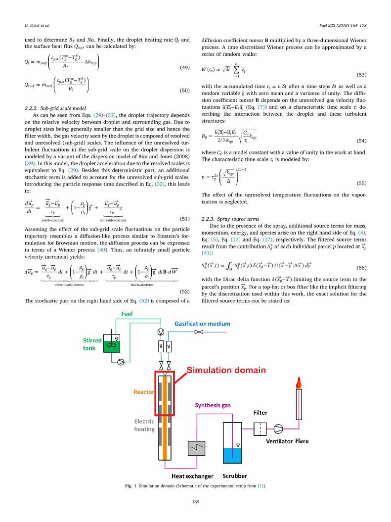
Fig. 1. Simulation domain (Schematic of the experimental setup from [1]).

G. Eckel et al. Fuel 223 (2018) 164–178

169

∑→ = →

=

S x tV

S x t( , ) 1 ( , )ϕd

f p

N

ϕp

1

p

(57)

This represents the volume-average of Np parcels in the filter volumeVf .In case of implicit filtering by the discretization, the filter volume Vf isequivalent to the cell volume Vcell. The mass change of the particles dueto evaporation or condensation leads to a mass source or sink term inthe gas field equations:

∑→ = −=

S x tV

dmdt

( , ) 1ρd

f p

Np

1

p

(58)

∑→ = −=

S x tV

d m Ydt

( , ) 1 ( )Yd

f p

Np p

α

1α

p

(59)

with the mass mp of the parcel p and the liquid mass fraction Y pα of

species α. A momentum source term arises due to changes in the par-cel’s momentum along its trajectory and due to forces acting on theparcel during a gas flow time step:

∑→ = − ⎛

⎝⎜

→−

⎯→⎯ ⎞

⎠⎟

=

S x tV

d m udt

F( , ) 1 ( )ρud

f p

Np p

1

p

(60)

wherein ⎯→⎯up represents the particle velocity vector and the second term

in Eq. (60) accounts for external forces⎯→⎯F affecting the particle, e.g. the

gravity force⎯→⎯

= →F m gg p . The energy source term yields:

∑ ∑→ = − ⎛

⎝⎜ +

→−

⎯→⎯ → ⎞

⎠⎟

= =

S x tV

d m Y edt

d m u

dtF u( , ) 1 ( ) ( | | )

·hd

f p

N

α

Np p

α α p pp

1 1

12

2p sp

(61)

The first term on the right hand side of Eq. (61) is the change of internalenergy e, the second term the change of kinetic energy and the third onethe work of external forces acting on the particle. The data are ex-changed online between the gaseous Eulerian phase and the liquidLagrangian phase via an iterative two-way-coupling procedure.

3. Test case and numerical setup

The testcase is the Research Entrained flow Gasifier (REGA) of theKarlsruhe Institute of Technology, Institute for Technical Chemistry(details see Part 1 of this paper series [1]). The atmospheric gasifierconsists of a tubular reactor with a length of 3.0m and an inner dia-meter of 0.28m. The liquid fuel (mono-ethylene glycol) is injected atthe top of the reactor via a twin-fluid atomizer [42]. The oxidizerconsists of oxygen-enriched air and serves as atomizing agent. Flangesand an axially movable burner allow for either intrusive or opticalmeasurements at different downstream distances from the nozzle exit.The side walls of the reactor are maintained at a constant temperatureby an electric heater. The simulation domain, highlighted in Fig. 1, wasdiscretized by a fully unstructured tetrahedral mesh. The grid was re-fined within the injector vanes, in the vicinity of the flame, and in nearwall regions. This led to a grid size of 2.7 million points correspondingto 15.9 million volume elements. Table 1 lists the boundary conditionsused in the LES of the REGA-glycol-T1 experiment. The input streamswere defined according to the set point defined in Table 4 of Part 1 ofthis paper series [1]. The purge nitrogen was neglected. Furthermore,the leakage air, which was determined by balancing (see Part 1) afterthe LES was almost completed, was not considered in this computation.This leads to slightly differing boundary conditions compared to Part 2[2] of this paper series. The starting conditions for the droplets werederived from Phase Doppler Anemometry (PDA). The twin-fluid ato-mizer produces a full cone spray. The droplet velocity and the liquidmass flow rate peak at the center and decrease towards larger radii.Details concerning the spray characterization can be found in Part 1 ofthis paper series [1]. The graphs indicate a slight w-shape and a Sautermean diameter ranging from 60 to 80μm. As measurements close to the

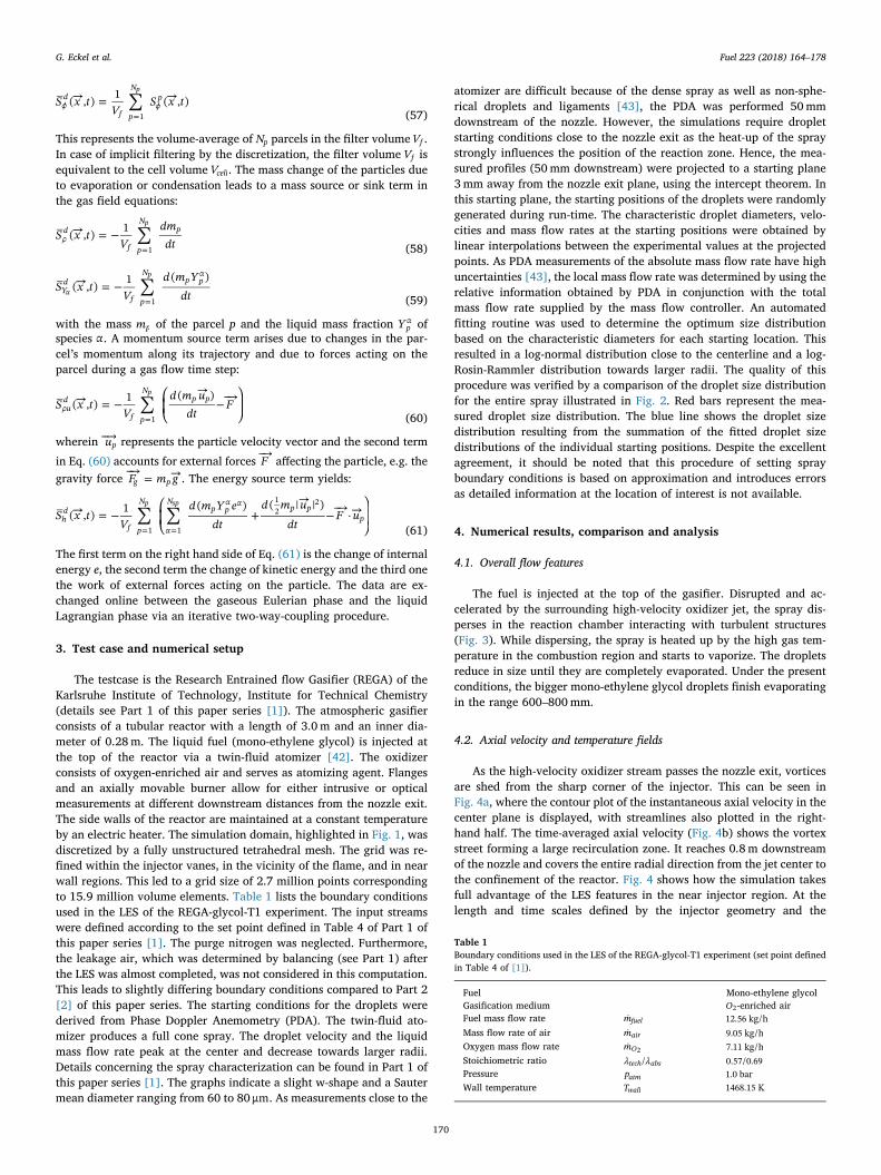
atomizer are difficult because of the dense spray as well as non-sphe-rical droplets and ligaments [43], the PDA was performed 50mmdownstream of the nozzle. However, the simulations require dropletstarting conditions close to the nozzle exit as the heat-up of the spraystrongly influences the position of the reaction zone. Hence, the mea-sured profiles (50mm downstream) were projected to a starting plane3mm away from the nozzle exit plane, using the intercept theorem. Inthis starting plane, the starting positions of the droplets were randomlygenerated during run-time. The characteristic droplet diameters, velo-cities and mass flow rates at the starting positions were obtained bylinear interpolations between the experimental values at the projectedpoints. As PDA measurements of the absolute mass flow rate have highuncertainties [43], the local mass flow rate was determined by using therelative information obtained by PDA in conjunction with the totalmass flow rate supplied by the mass flow controller. An automatedfitting routine was used to determine the optimum size distributionbased on the characteristic diameters for each starting location. Thisresulted in a log-normal distribution close to the centerline and a log-Rosin-Rammler distribution towards larger radii. The quality of thisprocedure was verified by a comparison of the droplet size distributionfor the entire spray illustrated in Fig. 2. Red bars represent the mea-sured droplet size distribution. The blue line shows the droplet sizedistribution resulting from the summation of the fitted droplet sizedistributions of the individual starting positions. Despite the excellentagreement, it should be noted that this procedure of setting sprayboundary conditions is based on approximation and introduces errorsas detailed information at the location of interest is not available.

4. Numerical results, comparison and analysis

4.1. Overall flow features

The fuel is injected at the top of the gasifier. Disrupted and ac-celerated by the surrounding high-velocity oxidizer jet, the spray dis-perses in the reaction chamber interacting with turbulent structures(Fig. 3). While dispersing, the spray is heated up by the high gas tem-perature in the combustion region and starts to vaporize. The dropletsreduce in size until they are completely evaporated. Under the presentconditions, the bigger mono-ethylene glycol droplets finish evaporatingin the range 600–800mm.

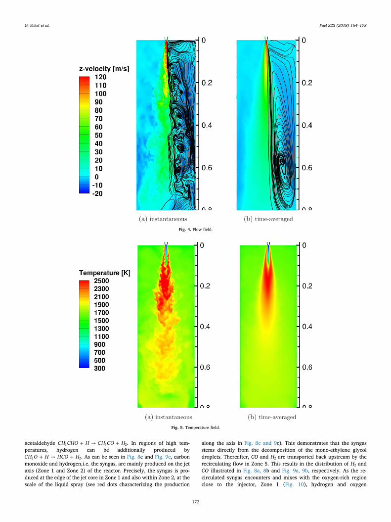
4.2. Axial velocity and temperature fields

As the high-velocity oxidizer stream passes the nozzle exit, vorticesare shed from the sharp corner of the injector. This can be seen inFig. 4a, where the contour plot of the instantaneous axial velocity in thecenter plane is displayed, with streamlines also plotted in the right-hand half. The time-averaged axial velocity (Fig. 4b) shows the vortexstreet forming a large recirculation zone. It reaches 0.8m downstreamof the nozzle and covers the entire radial direction from the jet center tothe confinement of the reactor. Fig. 4 shows how the simulation takesfull advantage of the LES features in the near injector region. At thelength and time scales defined by the injector geometry and the

Table 1Boundary conditions used in the LES of the REGA-glycol-T1 experiment (set point definedin Table 4 of [1]).

Fuel Mono-ethylene glycolGasification medium O2-enriched airFuel mass flow rate mfuel 12.56 kg/hMass flow rate of air mair 9.05 kg/hOxygen mass flow rate mO2 7.11 kg/hStoichiometric ratio λ λ/tech abs 0.57/0.69Pressure patm 1.0 barWall temperature Twall 1468.15 K

G. Eckel et al. Fuel 223 (2018) 164–178

170

incoming mass flow rate, the LES turbulence model captures the de-velopment of coherent structures. These coherent structures result veryrapidly in a highly unsteady turbulent mixing-layer and contributesubstantially to the local mixing between the incoming enriched air, therecirculating syngas, and the liquid fuel droplets. The time-averagedaxial velocity (Fig. 4b) is characterized by length and time scales closerto the integral scales of the reactor, thus closer to what one could expectfrom a RANS turbulence model (see Part 2 of this paper series). At in-tegral scales, the confined turbulent jet-flow is the main driver of therecirculation, which brings the gaseous components stemming from thechemical reactions along the jet axis back into the near injector region.Although the details of the twin-fluid atomizer (injection of liquid in themiddle and surrounding enriched-air impinging upon it [42]) departfrom a classical confined jet, from a fluid dynamics perspective the flowgenerated downstream the injector is qualitatively similar to it. TheReynolds number based on the hydraulic diameter of the nozzle and theaverage velocity through the nozzle annulus is equal to 28,800 (tur-bulent). Fig. 5 depicts the instantaneous (Fig. 5a) and time-averaged(Fig. 5b) temperature field in the center plane of the reaction chamber.From the flow patterns and the temperature field, five zones char-acterizing the near field of the injector can be defined:

1. Jet-flow along the axis close to the injector (0 < z<0.1m): Thisregion is the potential core of the jet, which expands radially and

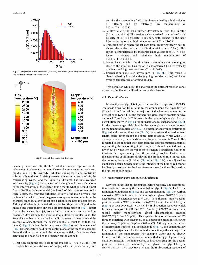
entrains the surrounding fluid. It is characterized by a high velocityof 110m/s and by relatively low temperatures of300 < T < 1500 K.

2. Jet-flow along the axis further downstream from the injector(0.1 < z < 0.4m): This region is characterized by a reduced axialvelocity of 40 < z-velocity < 100m/s, with respect to the nearinjector jet region and high temperatures of T > 2100 K.

3. Transition region where the jet goes from occupying nearly half toalmost the entire reactor cross-Section (0.4 < z < 0.8m). Thisregion is characterized by moderate axial velocities of 10 < z-ve-locity < 40m/s and relatively high temperatures of1500 < T < 2100 K.

4. Mixing-layer, which is the thin layer surrounding the incoming jetclose to the injector. This region is characterized by high velocitygradients and high temperatures (T > 2100 K).

5. Recirculation zone (see streamlines in Fig. 4b). This region ischaracterized by low velocities (e.g. high residence time) and by anaverage temperature of around 1500 K.

This definition will assist the analysis of the different reaction zonesas well as the flame stabilization mechanism later on.

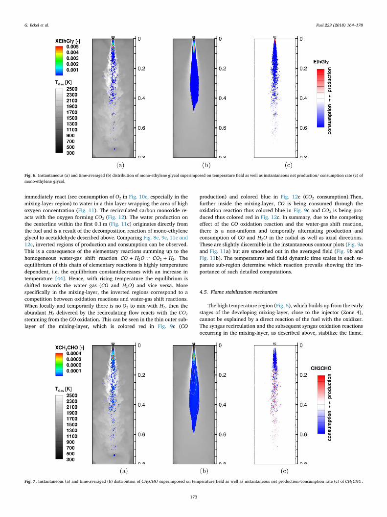
4.3. Vapor distribution

Mono-ethylene glycol is injected at ambient temperature (300 K).The phase transition from liquid to gas occurs along the expanding jet(Zone 1, 2, and 3). While the majority of the fuel evaporates in thepreheat zone (Zone 1) as the temperature rises, larger droplets surviveand reach Zone 2 and 3. This results in the mono-ethylene glycol vapordistribution shown in Fig. 6a for an instantaneous snapshot and Fig. 6bfor the time-averaged field; both in the center plane and superimposedon the temperature field of Fig. 5. The instantaneous vapor distribution(Fig. 6a) and consumption rates (Fig. 6c) demonstrate that predominantlength scales differ among the zones defined above. While Zone 1 isdensely populated, these fields have a discrete character in Zone 2. Thisis related to the fact that they stem from the discrete numerical parcelsrepresenting the evaporating liquid droplets. It should be noted that thelower cut-off value for the vapor mole fraction is arbitrarily chosen toillustrate the vapor coming from the surviving droplets. Furthermore,the color scale of all figures displaying the production rate (in red) andthe consumption rate (in blue) (Fig. 6c to Fig. 12c) was adjusted toemphasize details. Consequently, the intensity of the blue or red cannotbe directly correlated to the instantaneous mole fractions displayed onthe far left of each series.

4.4. Main reaction paths and species distributions

Ethylene glycol has to decompose before reacting. The decomposi-tion reactions consuming the mono-ethylene glycol (Fig. 6c) lead to theformation of hydrogen (Fig. 8c) and carbon monoxide (Fig. 9c). Carbonmonoxide (CO) is formed as mono-ethylene glycol (HOCH CH OH2 2 )decomposes to acetaldehyde (CH CHO3 ) in a thermal major decom-position reaction → +HOCH CH OH CH CHO H O2 2 3 2 . The acetaldehyde(Fig. 7) is then converted to CH CO3 by H-abstraction reactions whichfurther decomposes to CO (and CH3). Similarly, CH OH2 is formed in asecond major mono-ethylene glycol decomposition reaction( →HOCH CH OH CH OH22 2 2 ). This species is another source of COthrough reactions with oxygen O2 or H-abstraction reactions followingthe pathway → → →CH OH CH O CHO CO2 2 . Although concentrationsof intermediate species, e.g. acetaldehyde (Fig. 7), are comparativelylow, they are significant for the individual reaction paths leading to theformation of the main species. For example, water can be directlyformed from the decomposition of mono-ethylene glycol prior to anyoxidation reaction. The main sources of hydrogen (H2) are the decom-position reaction of mono-ethylene glycol to glycolaldehyde

→ +HOCH CH OH HOCH CHO H2 2 2 2 and the H-abstraction reactions of

Fig. 2. Comparison of the measured (red bars) and fitted (blue line) volumetric dropletsize distributions for the entire spray.

Fig. 3. Droplet dispersion and heat up.

G. Eckel et al. Fuel 223 (2018) 164–178

171

acetaldehyde + → +CH CHO H CH CO H3 3 2. In regions of high tem-peratures, hydrogen can be additionally produced by

+ → +CH O H HCO H2 2. As can be seen in Fig. 8c and Fig. 9c, carbonmonoxide and hydrogen,i.e. the syngas, are mainly produced on the jetaxis (Zone 1 and Zone 2) of the reactor. Precisely, the syngas is pro-duced at the edge of the jet core in Zone 1 and also within Zone 2, at thescale of the liquid spray (see red dots characterizing the production

along the axis in Fig. 8c and 9c). This demonstrates that the syngasstems directly from the decomposition of the mono-ethylene glycoldroplets. Thereafter, CO and H2 are transported back upstream by therecirculating flow in Zone 5. This results in the distribution of H2 andCO illustrated in Fig. 8a, 8b and Fig. 9a, 9b, respectively. As the re-circulated syngas encounters and mixes with the oxygen-rich regionclose to the injector, Zone 1 (Fig. 10), hydrogen and oxygen

Fig. 4. Flow field.

Fig. 5. Temperature field.

G. Eckel et al. Fuel 223 (2018) 164–178

172

immediately react (see consumption of O2 in Fig. 10c, especially in themixing-layer region) to water in a thin layer wrapping the area of highoxygen concentration (Fig. 11). The recirculated carbon monoxide re-acts with the oxygen forming CO2 (Fig. 12). The water production onthe centerline within the first 0.1 m (Fig. 11c) originates directly fromthe fuel and is a result of the decomposition reaction of mono-ethyleneglycol to acetaldehyde described above. Comparing Fig. 8c, 9c, 11c and12c, inverted regions of production and consumption can be observed.This is a consequence of the elementary reactions summing up to thehomogeneous water-gas shift reaction + ⇌ +CO H O CO H2 2 2. Theequilibrium of this chain of elementary reactions is highly temperaturedependent, i.e. the equilibrium constantdecreases with an increase intemperature [44]. Hence, with rising temperature the equilibrium isshifted towards the water gas (CO and H O2 ) and vice versa. Morespecifically in the mixing-layer, the inverted regions correspond to acompetition between oxidation reactions and water-gas shift reactions.When locally and temporarily there is no O2 to mix with H2, then theabundant H2 delivered by the recirculating flow reacts with the CO2stemming from the CO oxidation. This can be seen in the thin outer sub-layer of the mixing-layer, which is colored red in Fig. 9c (CO

production) and colored blue in Fig. 12c (CO2 consumption).Then,further inside the mixing-layer, CO is being consumed through theoxidation reaction thus colored blue in Fig. 9c and CO2 is being pro-duced thus colored red in Fig. 12c. In summary, due to the competingeffect of the CO oxidation reaction and the water-gas shift reaction,there is a non-uniform and temporally alternating production andconsumption of CO and H O2 in the radial as well as axial directions.These are slightly discernible in the instantaneous contour plots (Fig. 9aand Fig. 11a) but are smoothed out in the averaged field (Fig. 9b andFig. 11b). The temperatures and fluid dynamic time scales in each se-parate sub-region determine which reaction prevails showing the im-portance of such detailed computations.

4.5. Flame stabilization mechanism

The high temperature region (Fig. 5), which builds up from the earlystages of the developing mixing-layer, close to the injector (Zone 4),cannot be explained by a direct reaction of the fuel with the oxidizer.The syngas recirculation and the subsequent syngas oxidation reactionsoccurring in the mixing-layer, as described above, stabilize the flame.

Fig. 6. Instantaneous (a) and time-averaged (b) distribution of mono-ethylene glycol superimposed on temperature field as well as instantaneous net production/ consumption rate (c) ofmono-ethylene glycol.

Fig. 7. Instantaneous (a) and time-averaged (b) distribution of CH CHO3 superimposed on temperature field as well as instantaneous net production/consumption rate (c) of CH CHO3 .

G. Eckel et al. Fuel 223 (2018) 164–178

173

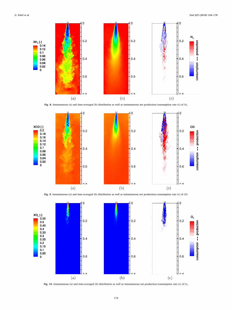
Fig. 8. Instantaneous (a) and time-averaged (b) distribution as well as instantaneous net production/consumption rate (c) of H2.

Fig. 9. Instantaneous (a) and time-averaged (b) distribution as well as instantaneous net production/consumption rate (c) of CO.

Fig. 10. Instantaneous (a) and time-averaged (b) distribution as well as instantaneous net production/consumption rate (c) of O2.

G. Eckel et al. Fuel 223 (2018) 164–178

174

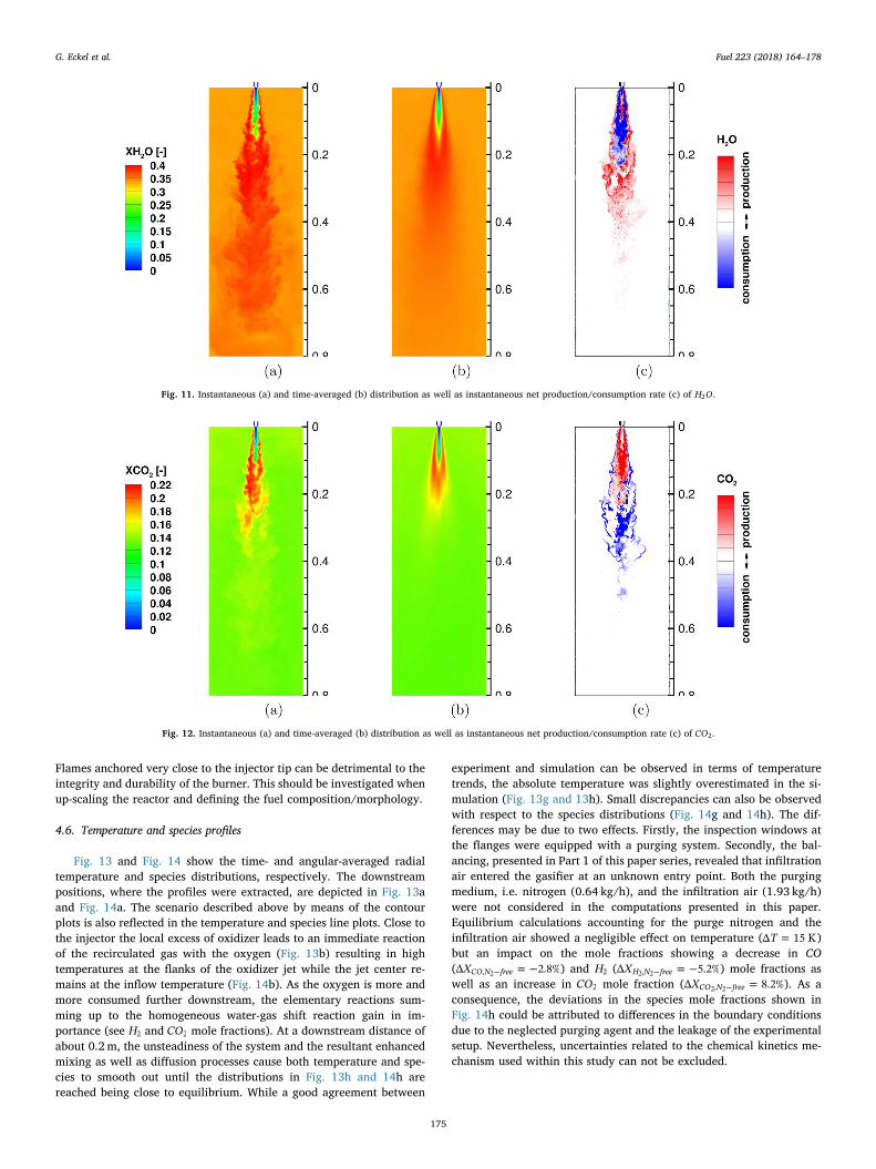
Flames anchored very close to the injector tip can be detrimental to theintegrity and durability of the burner. This should be investigated whenup-scaling the reactor and defining the fuel composition/morphology.

4.6. Temperature and species profiles

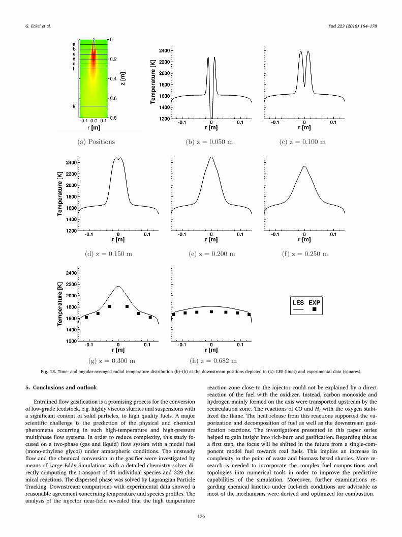
Fig. 13 and Fig. 14 show the time- and angular-averaged radialtemperature and species distributions, respectively. The downstreampositions, where the profiles were extracted, are depicted in Fig. 13aand Fig. 14a. The scenario described above by means of the contourplots is also reflected in the temperature and species line plots. Close tothe injector the local excess of oxidizer leads to an immediate reactionof the recirculated gas with the oxygen (Fig. 13b) resulting in hightemperatures at the flanks of the oxidizer jet while the jet center re-mains at the inflow temperature (Fig. 14b). As the oxygen is more andmore consumed further downstream, the elementary reactions sum-ming up to the homogeneous water-gas shift reaction gain in im-portance (see H2 and CO2 mole fractions). At a downstream distance ofabout 0.2m, the unsteadiness of the system and the resultant enhancedmixing as well as diffusion processes cause both temperature and spe-cies to smooth out until the distributions in Fig. 13h and 14h arereached being close to equilibrium. While a good agreement between

experiment and simulation can be observed in terms of temperaturetrends, the absolute temperature was slightly overestimated in the si-mulation (Fig. 13g and 13h). Small discrepancies can also be observedwith respect to the species distributions (Fig. 14g and 14h). The dif-ferences may be due to two effects. Firstly, the inspection windows atthe flanges were equipped with a purging system. Secondly, the bal-ancing, presented in Part 1 of this paper series, revealed that infiltrationair entered the gasifier at an unknown entry point. Both the purgingmedium, i.e. nitrogen (0.64 kg/h), and the infiltration air (1.93 kg/h)were not considered in the computations presented in this paper.Equilibrium calculations accounting for the purge nitrogen and theinfiltration air showed a negligible effect on temperature ( =TΔ 15 K)but an impact on the mole fractions showing a decrease in CO( = −−XΔ 2.8%CO N free, 2 ) and H2 ( = −−XΔ 5.2%H N free,2 2 ) mole fractions aswell as an increase in CO2 mole fraction ( =−XΔ 8.2%CO N free,2 2 ). As aconsequence, the deviations in the species mole fractions shown inFig. 14h could be attributed to differences in the boundary conditionsdue to the neglected purging agent and the leakage of the experimentalsetup. Nevertheless, uncertainties related to the chemical kinetics me-chanism used within this study can not be excluded.

Fig. 11. Instantaneous (a) and time-averaged (b) distribution as well as instantaneous net production/consumption rate (c) of H O2 .

Fig. 12. Instantaneous (a) and time-averaged (b) distribution as well as instantaneous net production/consumption rate (c) of CO2.

G. Eckel et al. Fuel 223 (2018) 164–178

175

5. Conclusions and outlook

Entrained flow gasification is a promising process for the conversionof low-grade feedstock, e.g. highly viscous slurries and suspensions witha significant content of solid particles, to high quality fuels. A majorscientific challenge is the prediction of the physical and chemicalphenomena occurring in such high-temperature and high-pressuremultiphase flow systems. In order to reduce complexity, this study fo-cused on a two-phase (gas and liquid) flow system with a model fuel(mono-ethylene glycol) under atmospheric conditions. The unsteadyflow and the chemical conversion in the gasifier were investigated bymeans of Large Eddy Simulations with a detailed chemistry solver di-rectly computing the transport of 44 individual species and 329 che-mical reactions. The dispersed phase was solved by Lagrangian ParticleTracking. Downstream comparisons with experimental data showed areasonable agreement concerning temperature and species profiles. Theanalysis of the injector near-field revealed that the high temperature

reaction zone close to the injector could not be explained by a directreaction of the fuel with the oxidizer. Instead, carbon monoxide andhydrogen mainly formed on the axis were transported upstream by therecirculation zone. The reactions of CO and H2 with the oxygen stabi-lized the flame. The heat release from this reactions supported the va-porization and decomposition of fuel as well as the downstream gasi-fication reactions. The investigations presented in this paper serieshelped to gain insight into rich-burn and gasification. Regarding this asa first step, the focus will be shifted in the future from a single-com-ponent model fuel towards real fuels. This implies an increase incomplexity to the point of waste and biomass based slurries. More re-search is needed to incorporate the complex fuel compositions andtopologies into numerical tools in order to improve the predictivecapabilities of the simulation. Moreover, further examinations re-garding chemical kinetics under fuel-rich conditions are advisable asmost of the mechanisms were derived and optimized for combustion.

Fig. 13. Time- and angular-averaged radial temperature distribution (b)–(h) at the downstream positions depicted in (a): LES (lines) and experimental data (squares).

G. Eckel et al. Fuel 223 (2018) 164–178

176

Acknowledgments

The research leading to these results has received funding from theHelmholtz Virtual Institute for Gasification Technology, HVIGasTech[45].

References

[1] Fleck S, Santo U, Hotz C, Jakobs T, Eckel G, Mancini M, Weber R, Kolb T. Entrainedflow gasification. Part 1: Gasification of glycol in an atmospheric-pressure experi-mental rig. Fuel 2018;217:306–19.

[2] Mancini M, Alberti M, Dammann M, Santo U, Eckel G, Kolb T et al. Entrained flowgasification. Part 2: Mathematical modeling of the gasifier using rans method, Fuel.

[3] Warnatz J, Maas U, Dibble R. Combustion – physical and chemical fundamentals,modeling and simulation, experiments, pollutant formation. 4th Edition BerlinHeidelberg: Springer; 2006.

[4] Gräbner M. Gasification of solids: past, present, and future. Wiley-VCH VerlagGmbH & Co. KGaA; 2014. Ch. 2, pp. 29–42.

[5] Pedel J, Thornock JN, Smith PJ. Large eddy simulation of pulverized coal jet flameignition using the direct quadrature method of moments. Energy Fuels2012;26(11):6686–94.

[6] Franchetti B, Marincola FC, Navarro-Martinez S, Kempf A. Large eddy simulation ofa pulverised coal jet flame. Proc Combust Inst 2013;34(2):2419–26.

[7] Stein O, Olenik G, Kronenburg A, Cavallo Marincola F, Franchetti B, Kempf A,Ghiani M, Vascellari M, Hasse C. Towards comprehensive coal combustion model-ling for LES. Flow Turbulence Combust 2013;90(4):859–84.

[8] Olenik G, Stein O, Kronenburg A. Les of swirl-stabilised pulverised coal combustionin {IFRF} furnace no. 1. Proc Combust Inst 2015;35(3):2819–28.

[9] Rabaçal M, Franchetti B, Marincola FC, Proch F, Costa M, Hasse C, Kempf A. Largeeddy simulation of coal combustion in a large-scale laboratory furnace. ProcCombust Inst 2015;35(3):3609–17.

[10] Boileau M, Pascaud S, Riber E, Cuenot B, Gicquel LYM, Poinsot TJ, Cazalens M.Investigation of two-fluid methods for large eddy simulation of spray combustion ingas turbines. Flow Turbulence Combust 2008;80(3):291–321.

[11] Patel N, Menon S. Simulation of spray-turbulence-flame interactions in a lean directinjection combustor. Combust Flame 2008;153(1-2):228–57.

[12] Chrigui M, Gounder J, Sadiki A, Masri AR, Janicka J. Partially premixed reactingacetone spray using {LES} and {FGM} tabulated chemistry. Combust Flame2012;159(8):2718–41 Special Issue on Turbulent Combustion.

[13] Ukai S, Kronenburg A, Stein O. LES-CMC of a dilute acetone spray flame. ProcCombust Inst 2013;34(1):1643–50.

[14] Sacomano Filho FL, Chrigui M, Sadiki A, Janicka J. LES-based numerical analysis ofdroplet vaporization process in lean partially premixed turbulent spray flames.Combust Sci Technol 2014;186(4–5):435–52.

Fig. 14. Time- and angular-averaged radial species mole fraction distributions (b)–(h) at the downstream positions depicted in (a): LES (lines) and experimental data (squares).

G. Eckel et al. Fuel 223 (2018) 164–178

177

[15] Heye C, Raman V, Masri AR. Influence of spray/combustion interactions on auto-ignition of methanol spray flames. Proc Combust Inst 2015;35(2):1639–48.

[16] Jones W, Marquis A, Vogiatzaki K. Large-eddy simulation of spray combustion in agas turbine combustor. Combust Flame 2014;161(1):222–39.

[17] Jones W, Marquis A, Noh D. LES of a methanol spray flame with a stochastic sub-grid model. Proc Combust Inst 2015;35(2):1685–91.

[18] Ghani A, Poinsot T, Gicquel L, Müller J-D. LES study of transverse acoustic in-stabilities in a swirled kerosene/air combustion chamber. Flow TurbulenceCombust 2016;96(1):207–26.

[19] Abani N, Ghoniem AF. Large eddy simulations of coal gasification in an entrainedflow gasifier. Fuel 2013;104:664–80.

[20] Löwe J, Probst A, Knopp T, Kessler R. A low-dissipation low-dispersion second-order scheme for unstructured finite-volume flow solvers. In: 53rd AIAA AerospaceSciences Meeting, Kissimmee, Florida; 2015.

[21] Sagaut P, Deck S, Terracol M. Multiscale and multiresolution approaches in tur-bulence. Imperial College Press; 2006.

[22] Pope S. Turbulent flows. Cambridge: Cambridge University Press; 2000.[23] Fröhlich J. Large Eddy Simulation turbulenter Strömungen. B.G: Teubner Verlag/

GWV Fachverlage GmbH; 2006.[24] Poinsot T, Veynante D. Theoretical and numerical combustion. 3rd ed. Toulouse:

CNRS; 2011.[25] Gerlinger P. Numerische Verbrennungssimulation – Effiziente numerische

Simulation turbulenter Verbrennung. Berlin: Springer; 2005.[26] Noll B. Möglichkeiten und Grenzen der numerischen Beschreibung von Strömungen

in hochbelasteten Brennräumen. Universität Karlsruhe; 1992.[27] Ducros F, Nicoud F, Poinsot T. A wall-adapting local eddy-viscosity model for si-

mulations in complex geometries. In: Conference on Numerical Methods for FluidDynamics, Oxford, UK; 1998.

[28] Nicoud F, Ducros F. Subgrid-scale stress modelling based on the square of the ve-locity gradient tensor. Flow Turbulence Combust 1999;62(3):183–200.

[29] Boussinesq J. Essai sur la théorie des eaux courantes. Rapport sur un mémoire de M.Boussinesq, Mémoires présentés par divers savants à l’Académie des sciences del’Institut de France: sciences mathématiques et physiques 1 (1877) XXII–680.

[30] Probst A, Löwe J, Reu S, Knopp T, Kessler R. Scale-resolving simulations with a low-dissipation low-dispersion second-order scheme for unstructured finite-volume flowsolvers. In: 53rd AIAA Aerospace Sciences Meeting, Kissimmee, Florida; 2015.

[31] Di Domenico M. Numerical simulations of soot formation in turbulent flows Ph.D.

thesis Fakultät für Luft- und Raumfahrttechnik und Geodäsie, Universität Stuttgart;2008.

[32] Ivanova E. Numerical simulations of turbulent mixing in complex flows Ph.D. thesisInstitute of Combustion Technology for Aerospace Engineering, University ofStuttgart; 2012.

[33] Kuo KK. Principles of combustion. New York: Wiley; 1986.[34] Hafner S. Modellentwicklung zur numerischen simulation eines flugstromvergasers

für biomasse. Ruprechts-Karls-Universität Heidelberg; 2010. [Ph.D. thesis].[35] Hafner S, Rashidi A, Baldea G, Riedel U. A detailed chemical kinetic model of high-

temperature ethylene glycol gasification. Combust Theor Model2011;15(4):517–35.

[36] Kathrotia T, Naumann C, Owald P, Köhler M, Riedel U. Kinetics of ethylene glycol:the first validated reaction scheme and first measurements of ignition delay timesand speciation data. Combust Flame 2017;179:172–84.

[37] Abramzon B, Sirignano W. Droplet vaporization model for spray combustion cal-culations. Int J Heat Mass Transfer 1989;32(9):1605–18.

[38] Clift R, Grace JR, Weber ME. Bubbles, drops, and particles. New York: AcademicPress; 1978.

[39] Bini M, Jones WP. Large-eddy simulation of particle-laden turbulent flows. J FluidMech 2008;614:207–52.

[40] Gardiner CW. Handbook of stochastic methods: for physics, chemistry and thenatural sciences. 3rd ed. Berlin; Heidelberg [u.a.]: Springer; 2004.

[41] Leboissetier A, Okong’o N, Bellan J. Consistent large-eddy simulation of a temporalmixing layer laden with evaporating drops. Part 2. a posteriori modelling. J FluidMech 2005;523:37–78.

[42] Jakobs T, Djordjevic N, Fleck S, Mancini M, Weber R, Kolb T. Gasification of highviscous slurry R&D on atomization and numerical simulation. Appl Energy2012;93:449–56.

[43] Tropea C. Optical particle characterization in flows. Annu Rev Fluid Mech2011;43(1):399–426.

[44] Bustamante F, Enick RM, Cugini A, Killmeyer RP, Howard BH, Rothenberger KS,Ciocco MV, Morreale BD, Chattopadhyay S, Shi S. High-temperature kinetics of thehomogeneous reverse water-gas shift reaction. AIChE J 2004;50(5):1028–41.

[45] Kolb T, Aigner M, Kneer R, Müller M, Weber R, Djordjevic N. Tackling the chal-lenges in modelling entrained-flow gasification of low-grade feedstock. J EnergyInst 2016;89(4):485–503.

G. Eckel et al. Fuel 223 (2018) 164–178

178