entity-oriented data science - nist · · 2013-09-05" entity resolution – clustering nodes...

Entity-Oriented Data Science

Prof. Lise Getoor University of Maryland, College Park

http://www.cs.umd.edu/~getoor

September 5, 2013

Data is not flat BIG

©2004-2013 lonnitaylor

Entities and relationships are important!

Data is multi-modal, multi-relational, spatio-temporal, multi-media

NEED: Data Science for Graphs

Statistical Relational Learning (SRL) ¢  AI/DB representations + statistics for multi-relational data

l  Entities can be of different types l  Entities can participate in a variety of relationships l  examples: Markov logic networks, relational dependency networks,

Bayesian logic programs, probabilistic relational models, many others…..

¢  Key ideas l  Relational feature construction l  Collective reasoning l  ‘Lifted’ representation, inference and learning

¢  Related areas

l  structured prediction, hierarchical models, latent-variable relational models, multi-relational tensors, representation learning, …

For more details, see NIPS 2012 Tutorial, ��http://linqs.cs.umd.edu/projects//Tutorials/nips2012.pdf

Common Graph Data Analysis Patterns

¢  Joint inference over large networks for:

l  Collective Classification – inferring labels of nodes in graph

l  Link Prediction – inferring the existence of edges in graph

l  Entity Resolution – clustering nodes that refer to the same underlying entity

Common Graph Data Analysis Patterns

¢  Joint inference over large networks for: l  Collective Classification – inferring labels of nodes

in graph

l  Link Prediction – inferring the existence of edges in graph

l  Entity Resolution – clustering nodes that refer to the same underlying entity

What’s Needed Next? ¢  Methods which can perform and interleave these

tasks ¢  Methods which support:

l  Graph identification – inferring a graph from noisy observations

l  Graph alignment - mapping components in one graph to another

l  Graph summarization - clustering the nodes and edges in a graph

¢  Desiderata: Flexible, scalable, declarative support for collective classification, link prediction, entity resolution and other information alignment and information fusion problems….

Probabilistic Soft Logic (PSL)

Matthias Broecheler Lily Mihalkova Stephen Bach Stanley Kok Alex Memory

Bert Huang Angelika Kimmig

http://psl.umiacs.umd.edu

Probabilistic Soft Logic (PSL) Declarative language based on logics to express

collective probabilistic inference problems -  Predicate = relationship or property -  Atom = (continuous) random variable -  Rule = capture dependency or constraint -  Set = define aggregates

PSL Program = Rules + Input DB


Node Labeling

?


Voter Opinion Modeling

? $ $

Tweet Status update



spouse

spouse

colleague

colleague

spouse friend

friend

friend

friend



vote(A,P) ∧ spouse(B,A) à vote(B,P) : 0.8

vote(A,P) ∧ friend(B,A) à vote(B,P) : 0.3

spouse

spouse

colleague

colleague

spouse friend

friend

friend

friend


Link Prediction §  Entities

-  People, Emails

§  Attributes -  Words in emails

§  Relationships -  communication, work

relationship

§  Goal: Identify work relationships

-  Supervisor, subordinate, colleague

#


Link Prediction § People, emails, words,

communication, relations § Use rules to express

evidence -  “If email content suggests type X, it

is of type X” -  “If A sends deadline emails to B,

then A is the supervisor of B” -  “If A is the supervisor of B, and A is

the supervisor of C, then B and C are colleagues”

#








#

complete by

due








#


Entity Resolution § Entities

-  People References

§ Attributes -  Name

§ Relationships -  Friendship

§ Goal: Identify references that denote the same person

A B

John Smith J. Smith

name name

C

E

D F G

H

friend friend

=

=


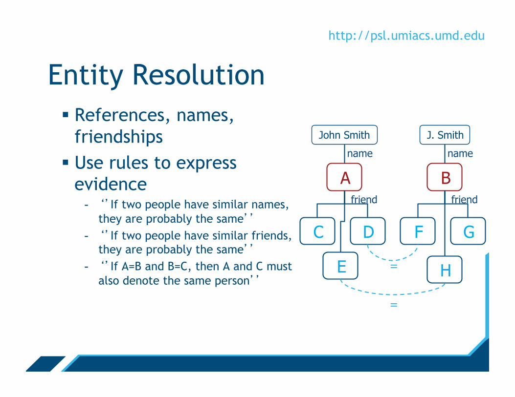
Entity Resolution § References, names,

friendships § Use rules to express

evidence -  ‘’If two people have similar names,

they are probably the same’’ -  ‘’If two people have similar friends,

they are probably the same’’ -  ‘’If A=B and B=C, then A and C must

also denote the same person’’

A B

John Smith J. Smith

name name

C

E

D F G

H

friend friend

=

=








A B

John Smith J. Smith

name name

C

E

D F G

H

friend friend

=

=

A.name ≈{str_sim} B.name => A≈B : 0.8








A B

John Smith J. Smith

name name

C

E

D F G

H

friend friend

=

=

{A.friends} ≈{} {B.friends} => A≈B : 0.6








A B

John Smith J. Smith

name name

C

E

D F G

H

friend friend

=

=

A≈B ^ B≈C => A≈C : ∞


Logic Foundation


Rules

§ Atoms are real valued -  Interpretation I, atom A: I(A) [0,1] -  We will omit the interpretation and write A [0,1]

§ ∨, ∧ are combination functions -  T-norms: [0,1]n →[0,1]

H1 ∨... Hm ← B1 ∧ B2 ∧ ... Bn

Ground Atoms [Broecheler, et al., UAI ‘10]


Rules

§ Combination functions (Lukasiewicz T-norm) § A ∨ B = min(1, A + B) § A ∧ B = max(0, A + B – 1)

H1 ∨... Hm ← B1 ∧ B2 ∧ ... Bn

[Broecheler, et al., UAI ‘10]


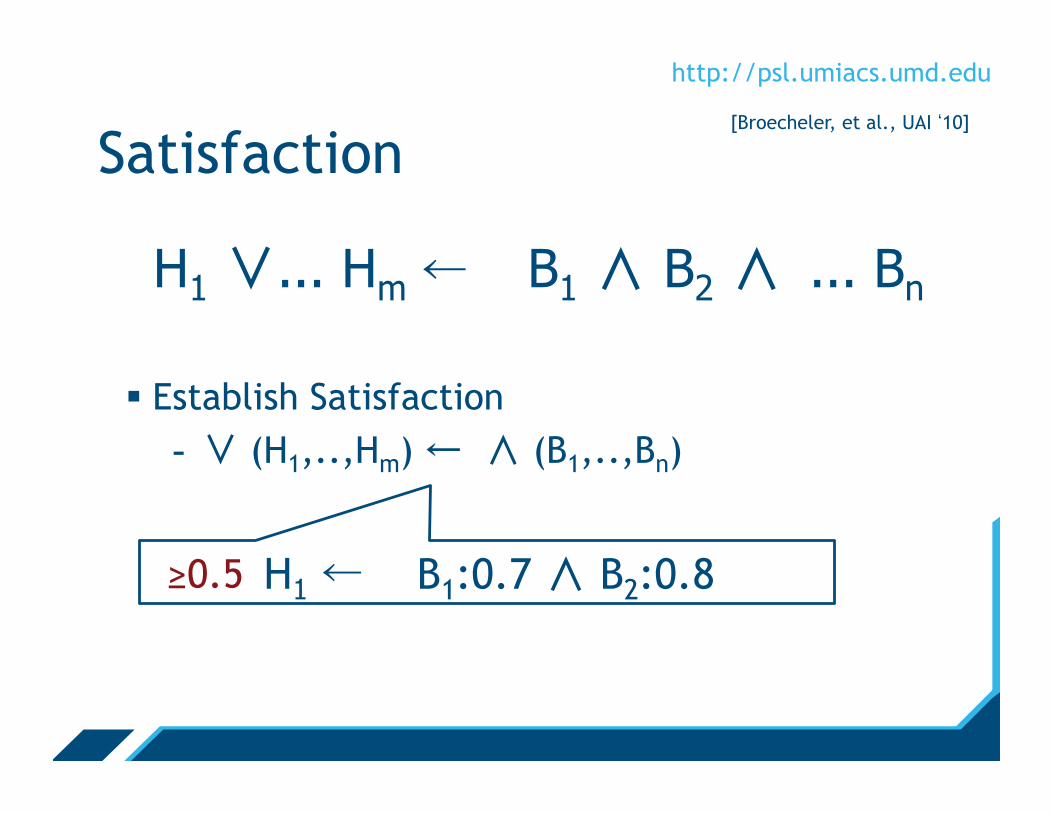
Satisfaction

§ Establish Satisfaction -  ∨ (H1,..,Hm) ← ∧ (B1,..,Bn)

H1 ∨... Hm ← B1 ∧ B2 ∧ ... Bn

H1 ← B1:0.7 ∧ B2:0.8


≥0.5


Distance to Satisfaction

§ Distance to Satisfaction

-  max( ∧ (B1,..,Bn) - ∨ (H1,..,Hm) , 0)

H1 ∨... Hm ← B1 ∧ B2 ∧ ... Bn

H1:0.7 ← B1:0.7 ∧ B2:0.8

H1:0.2 ← B1:0.7 ∧ B2:0.8

0.0

0.3



W: H1 ∨... Hm ← B1 ∧ B2 ∧ ... Bn

Rule Weights

§ Weighted Distance to Satisfaction -  d(R,I) = W � max( ∧ (B1,..,Bn) - ∨ (H1,..,Hm) , 0)



So far….

§ Given a data set and a PSL program, we can construct a set of ground rules.

§ Some of the atoms have fixed truth values and some have unknown truth values.

§ For every assignment of truth values to the unknown atoms, we get a set of weighted distances from satisfaction.

§ How to decide which is best?


Probabilistic Foundation


Probabilistic Model Probability

density over interpretation I

Normalization constant

Ground rules Distance exponent (in {1, 2})

Ground rule’s distance to satisfaction

Rule weight

P (I) =1

Zexp

"�X

r2R

wr(dr(I))pr

#dr(I) = max{Ir,body � Ir,head, 0}


Hinge-loss MRFs


Hinge-loss Markov Random Fields

P (Y |X) =

1

Zexp

2

4�mX

j=1

wj max{`j(Y,X), 0}pj

3

5

§ Continuous variables in [0,1] § Potentials are hinge-loss functions § Subject to arbitrary linear constraints § Log-concave!


Inference as Convex Optimization § Maximum Aposteriori Probability (MAP) Objective:

§ This is convex! § Can solve using off-the-shelf convex optimization

packages § … or custom solver

argmax

YP (Y |X)

= argmin

Y

mX

j=1

wj max{`j(Y,X), 0}pj


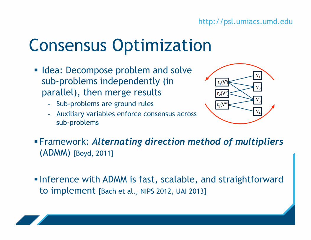
Consensus Optimization §  Idea: Decompose problem and solve

sub-problems independently (in parallel), then merge results

-  Sub-problems are ground rules -  Auxiliary variables enforce consensus across

sub-problems

§ Framework: Alternating direction method of multipliers (ADMM) [Boyd, 2011]

§ Inference with ADMM is fast, scalable, and straightforward to implement [Bach et al., NIPS 2012, UAI 2013]


Speed

§  Inference in HL-MRFs is orders of magnitude faster than in discrete MRFs which use MCMC approximate inference

§  In practice, scales linearly with the number of potentials

Cora Citeseer Epinions Ac/vity Discrete MRF 110.9 s 184.3 s 212.4 s 344.2 s HL-‐MRF 0.4 s 0.7 s 1.2 s 0.6 s

[Bach et al., UAI 2013; London et al., 2013]

Average running time


Compiling PSL à HL-MRF §  Ground out first-order rules

-  Variables: soft-truth values of atoms -  Hinge-loss potentials: weighted distances to

satisfaction of ground rules

§ 

§  The effect is assignments that satisfy weighted rules more are more probable

w : A ! B

w : ¬A _ B

w ⇥ (1�min{1� A+ B , 1})w ⇥max{A� B , 0}


Inference Meta-Algorithm

51

Each ground rule constitutes a linear or

conic constraint, introducing a rule-

specific “dissatisfaction” variable that is added to the objective function.



52

Find most probable assignment using

consensus optimization (ADMM) subroutine



53

Conservative Grounding: Most rules trivially have satisfaction distance=0. Save time and space by not grounding them out

in the first place.

Don’t reason about it if you don’t absolutely have to!

Distributed MAP Inference §  ADMM consensus optimization problem can be implemented

naturally in distributed setting §  For k+1 iteration, it consists three steps in which sub problems

can run independently (1st and 2nd step): 1.  Update Lagrangian multiplier

2.  Update each sub problem

3.  Update the global variables

.

.

.

.

.

.

.

.

.

.

.

.

OR

Miao, Liu, Huang, Getoor, IEEE Big Data 2013

Distributed MAP: MapReduce

z1z1 zq zqz1 z2

��

z2 zp

��subproblem

local variable

copy

Mapper

z1 z2z1 z1 z2 zq zq zp��

Reducerupdate global

component

load global variable X as side dataJob Bootstrap

HDFS or HBase

read/write subproblem

write new global variable

read global variable X

Pros: •  Straightforward Design Cons: •  Job bootstrapping cost

between iterations •  Difficult to schedule

subset of nodes to run.

Distributed MAP: GraphLab

.

.

.

.

.

.

.

.

.

.

.

.

subproblem

node

global variable component

gather get z

apply update y update x

scatter notify z

gather get local z,y

apply update z

scatter unless converge notify X

update i update i+1

Advantages: •  No need to touch disk, no

job bootstrap-ping cost •  Easy to express local

convergence conditions to schedule only subset of nodes.

Experimental Results §  Using PSL for knowledge graph cleaning task

-  16M+ vertices, 22M+ edges, for small running instances -  Takes 100 minutes to finish in Java single machine

implementation using 40G+ memory -  Distributed GraphLab implementation takes less than 15

minutes using 4 smaller machines -  Possible to use commodity machines on large models!

Experimental Results Voter model using commodity machines

Name |Subproblem| |Consensus| |Edge| Fit in One Machine?

Run time (sec) |m| = 8

SN1M 3.3M 1.1M 6M Yes 2230

SN2M 6.6M 2.1M 12M No 3997

SN3M 10M 3.1M 18M No 4395

SN4M 13M 4.2M 24M No 5376

2000 3000 4000 5000 6000 7000 8000 9000

2 4 6 8

Run

ning

tim

e (s

ec)

Number of machines

HyperGreedy

Weak scaling with increasing size

500 1000 1500 2000 2500 3000 3500 4000 4500 5000 5500

2 4 6 8

Run

ning

tim

e (s

ec)

Number of Machines (SN2M)

HyperGreedy

Strong scaling with fixed dataset

Machine: Intel Core2 Quad CPU 2.66GHz machines �� with 4GB RAM running Ubuntu 12.04 Linux

Miao, Liu, Huang, Getoor, BigData ’13


Weight Learning


Weight Learning § Learn from training data

§ No need to hand-code rule-weights

§ Various methods: -  approximate maximum likelihood

- maximum pseudo-likelihood

-  large-margin estimation Bach, et al., UAI 2013

[Broecheler et al., UAI ’10]


Weight Learning § State-of-the-art supervised-learning performance on -  Collective classification -  Social-trust prediction -  Preference prediction -  Image reconstruction


Example PSL Program


Collective Activity Detection

Talking Talking Waiting

Walking

§  Objective: Classify actions of individuals in a video sequence -  Requires tracking the multiple targets, performing ID maintenance


Incorporate Low-level Detectors Histogram of Oriented Gradients (HOG) [Dalal & Triggs, CVPR 2005]

Action Context Descriptors (ACD) [Lan et al., NIPS 2010]

For each action a, define PSL rule:

wlocal,a : Doing(X, a) ← Detector(X, a)

wlocal,walking : Doing(X, walking) ← Detector(X, walking) e.g.,


Easily Encode Intuitions §  Proximity: People that are close (in frame)

are likely doing the same action

-  Closeness is measured via a radial basis function

§  Proximity: People are likely to continue doing the same action

-  Requires tracking & ID maintenance rule:

wprox,a : Doing(X, a) ← Close(X, Y) ∧ Doing(Y, a)

wpersist,a : Doing(Y, a) ← Same (X, Y) ∧ Doing(X, a)

wid : Same(X, Y) ← Sequential(X, Y) ∧ Close(X, Y)


Other Rules § Action transitions § Frame/scene consistency § Priors § (Partial-)Functional Constraints


Collective Activity Detection Model

wid : Same(X, Y) ← Sequential(X, Y) ∧ Close(X, Y)

widprior : ~SamePerson(X, Y)

For all actions a:

wlocal,a : Doing(X, a) ← Detector(X, a)

wframe,a : Doing(X, a) ← Frame(X, F) ∧ FrameAction(F, a)

wprox,a : Doing(X, a) ← Close(X, Y) ∧ Doing(Y, a)

wpersist,a : Doing(Y, a) ← SamePerson(X, Y) ∧ Doing(X, a)

wprior,a : ~Doing(X, a)

[London et al., 2013]


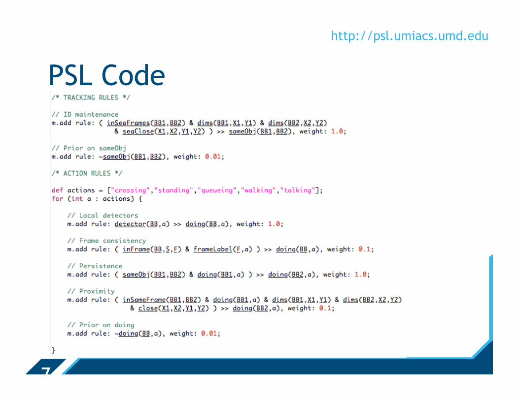
PSL Code

73


PSL Code

74


PSL Code

75


Foundations Summary


Foundations Summary § Design probabilistic models using

declarative language -  Syntax based on first-order logic

§ Inference of most-probable explanation is fast convex optimization (ADMM)

§ Learning algorithms for training rule weights from labeled data


PSL Applications


Document Classification

2

2 2

2 2 A

B

A or B?

A or B? A or B?

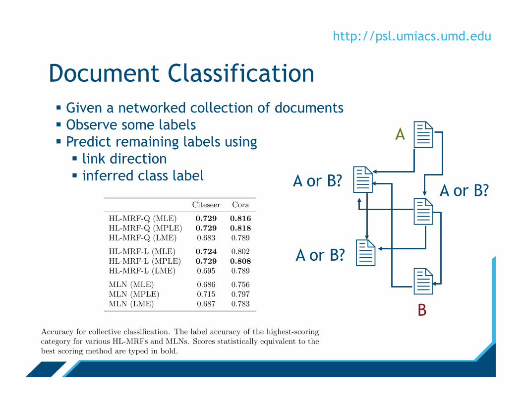
§  Given a networked collection of documents §  Observe some labels §  Predict remaining labels using

§  link direction §  inferred class label

Citeseer Cora

HL-MRF-Q (MLE) 0.729 0.816HL-MRF-Q (MPLE) 0.729 0.818HL-MRF-Q (LME) 0.683 0.789

HL-MRF-L (MLE) 0.724 0.802HL-MRF-L (MPLE) 0.729 0.808HL-MRF-L (LME) 0.695 0.789

MLN (MLE) 0.686 0.756MLN (MPLE) 0.715 0.797MLN (LME) 0.687 0.783

Accuracy for collective classification. The label accuracy of the highest-scoringcategory for various HL-MRFs and MLNs. Scores statistically equivalent to thebest scoring method are typed in bold.


Computer Vision Applications § Low-level vision:

-  image reconstruction

§ High-level vision: -  activity recognition in videos

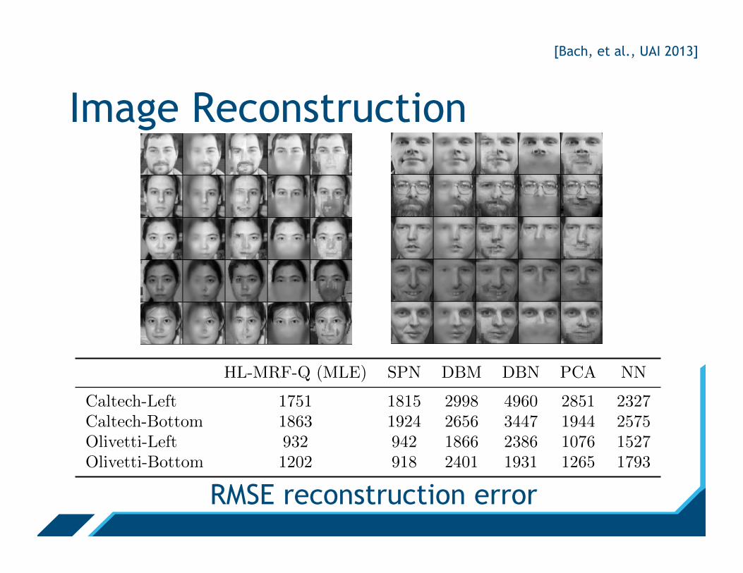
Image Reconstruction

Table 5: Mean squared errors per pixel for image reconstruction. HL-MRFs produce the most accurate recon-structions on the Caltech101 and the left-half Olivetti faces, and only sum-product networks produce betterreconstructions on Olivetti bottom-half faces. Scores for other methods are taken from Poon and Domingos [18].

HL-MRF-Q (MLE) SPN DBM DBN PCA NN

Caltech-Left 1751 1815 2998 4960 2851 2327Caltech-Bottom 1863 1924 2656 3447 1944 2575Olivetti-Left 932 942 1866 2386 1076 1527Olivetti-Bottom 1202 918 2401 1931 1265 1793

Figure 1: Example results on image reconstruction of Caltech101 (left) and Olivetti (right) faces. From leftto right in each column: (1) true face, left side predictions by (2) HL-MRFs and (3) SPNs, and bottom halfpredictions by (4) HL-MRFs and (5) SPNs. SPN reconstructions are downloaded from Poon and Domingos [18].

Table 5. HL-MRFs produce the best mean squarederror on the left- and bottom-half settings for the Cal-tech101 set and the left-half setting in the Olivetti set.Only sum product networks produce lower error onthe Olivetti bottom-half faces. Some reconstructedfaces are displayed in Figure 1, where that the shallow,pixel-based HL-MRFs produce comparably convinc-ing images to sum-product networks, especially in theleft-half setting, where HL-MRF can learn which pix-els are likely to mimic their horizontal mirror. Whileneither method is particularly good at reconstructingthe bottom half of faces, the qualitative di↵erence be-tween the deep SPN and the shallow HL-MRF recon-structions is that SPNs seem to hallucinate di↵erentfaces, often with some artifacts, while HL-MRFs pre-dict blurry shapes roughly the same pixel intensity asthe observed, top half of the face. The tendency tobetter match pixel intensity helps HL-MRFs score bet-ter quantitatively on the Caltech101 faces, where thelighting conditions are more varied than in Olivetti.

Training and predicting with these pixel-based HL-MRFs takes little time. In our experiments, training

takes about 1.5 hours on a 24-core machine, while pre-dicting takes about a second per image. While Poonand Domingos [18] report faster training with SPNs,both HL-MRFs and SPNs clearly belong to a class offaster models when compared to DBNs and DBMs,which can take days to train on modern hardware.

6 CONCLUSION

We have shown that HL-MRFs are a flexible and in-terpretable class of models, capable of modeling awide variety of domains. HL-MRFs admit fast, con-vex inference, because their density functions are log-concave. The MPE inference algorithm we introduceis applicable to the full class of HL-MRFs. With thisfast, general algorithm, we are the first to show resultsusing quadratic HL-MRFs on real-world data. In ourexperiments, HL-MRFs match or exceed the predic-tive performance of state-of-the-art methods on fourdiverse tasks. The natural mapping between hinge-loss potentials and logic rules makes HL-MRFs easyto define and interpret.

RMSE reconstruction error

[Bach, et al., UAI 2013]

Activity Recognition in Videos

crossing waiting queueing walking talking dancing jogging

[London, et al., CVPR WS 2013]

432433434435436437438439440441442443444445446447448449450451452453454455456457458459460461462463464465466467468469470471472473474475476477478479480481482483484485

486487488489490491492493494495496497498499500501502503504505506507508509510511512513514515516517518519520521522523524525526527528529530531532533534535536537538539

CVPR#3

CVPR#3

CVPR 2013 Submission #3. CONFIDENTIAL REVIEW COPY. DO NOT DISTRIBUTE.

is used for identity maintenance and tracking. It essentiallysays that if two bounding boxes occur in adjacent framesand their positions have not changed significantly, then theyare likely the same actor. We then reason, in R5, that if twobounding boxes (in adjacent frames) refer to the same actor,then they are likely to be doing the same activity. Note thatrules are defined for each action, such that we can learn dif-ferent weights for different actions. We define priors overthe predicates SAME and DOING, which we omit for space.We also define (partial) functional constraints (not shown),such that the truth-values over all actions (respectively, overall adjacent bounding boxes), sum to (at most) one. Wetrain the weights for these rules using 50 iterations of votedperceptron, with a step size of 0.1.

Note that we perform identity maintenance only to im-prove our activity predictions. During prediction, we do notobserve the SAME predicate, so we have to predict it. Wethen use these predictions to inform the rules pertaining toactivities.

4.3. Experiments

To illustrate the lift one can achieve on low-level predic-tors, we evaluate two versions of our model: the first usesactivity beliefs from predictions on the HOG features; thesecond uses activity beliefs predicted on the AC descrip-tors. Essentially, this determines which low-level predic-tions are used in the predicates LOCAL and FRAMELA-BEL. We denote these models by HL-MRF + HOG and HL-MRF + ACD respectively. We compare these to the pre-dictions made by the first-stage predictor (HOG) and thesecond-stage predictor (ACD).

The results of these experiments are listed in Table 1. Wealso provide recall matrices (row-normalized confusion ma-trices) for HL-MRF + ACD in Figure 2. For each dataset,we use leave-one-out cross-validation, where we train ourmodel on all except one sequence, then evaluate our predic-tions on the hold-out sequence. We report cumulative ac-curacy and F1 to compensate for skew in the size and labeldistribution across sequences. This involves accumulatingthe confusion matrices across folds.

Our results illustrate that our models are able to achievesignificant lift in accuracy and F1 over the low-level detec-tors. Specifically, we see that HL-MRF + HOG achieves a12 to 20 point lift over the baseline HOG model, and HL-MRF + ACD obtains a 1.5 to 2.5 point lift over the ACDmodel.

5. ConclusionWe have shown that HL-MRFs are a powerful class of

models for high-level computer vision tasks. When com-bined with PSL, designing probabilistic models is easy andintuitive. We applied these models to the task of collec-tive activity detection, building on local, low-level detectors

Table 1. Results of experiments with the 5- and 6-activity datasets,using leave-one-out cross-validation. The first dataset contains 44sequences; the second, 63 sequences. Scores are reported as thecumulative accuracy/F1, to account for size and label skew acrossfolds.

5 Activities 6 ActivitiesMethod Acc. F1 Acc. F1HOG .474 .481 .596 .582HL-MRF + HOG .598 .603 .793 .789ACD .675 .678 .835 .835HL-MRF + ACD .692 .693 .860 .860

Figure 2. Recall matrices (i.e., row-normalized confusion matri-ces) for the 5- and 6-activity datasets, using the HL-MRF + ACDmodel.

to create a global, relational model. Using simple, inter-pretable first-order logic rules, we were able to improve theaccuracy of low-level detectors.

References[1] M. R. Amer, D. Xie, M. Zhao, S. Todorovic, and S. C. Zhu,

“Cost-sensitive top-down/bottom-up inference for multiscaleactivity recognition,” in European Conference on ComputerVision, 2012. 1

5

Results on Activity Recognition

432433434435436437438439440441442443444445446447448449450451452453454455456457458459460461462463464465466467468469470471472473474475476477478479480481482483484485

486487488489490491492493494495496497498499500501502503504505506507508509510511512513514515516517518519520521522523524525526527528529530531532533534535536537538539

CVPR#3

CVPR#3

CVPR 2013 Submission #3. CONFIDENTIAL REVIEW COPY. DO NOT DISTRIBUTE.

is used for identity maintenance and tracking. It essentiallysays that if two bounding boxes occur in adjacent framesand their positions have not changed significantly, then theyare likely the same actor. We then reason, in R5, that if twobounding boxes (in adjacent frames) refer to the same actor,then they are likely to be doing the same activity. Note thatrules are defined for each action, such that we can learn dif-ferent weights for different actions. We define priors overthe predicates SAME and DOING, which we omit for space.We also define (partial) functional constraints (not shown),such that the truth-values over all actions (respectively, overall adjacent bounding boxes), sum to (at most) one. Wetrain the weights for these rules using 50 iterations of votedperceptron, with a step size of 0.1.

Note that we perform identity maintenance only to im-prove our activity predictions. During prediction, we do notobserve the SAME predicate, so we have to predict it. Wethen use these predictions to inform the rules pertaining toactivities.

4.3. Experiments

To illustrate the lift one can achieve on low-level predic-tors, we evaluate two versions of our model: the first usesactivity beliefs from predictions on the HOG features; thesecond uses activity beliefs predicted on the AC descrip-tors. Essentially, this determines which low-level predic-tions are used in the predicates LOCAL and FRAMELA-BEL. We denote these models by HL-MRF + HOG and HL-MRF + ACD respectively. We compare these to the pre-dictions made by the first-stage predictor (HOG) and thesecond-stage predictor (ACD).

The results of these experiments are listed in Table 1. Wealso provide recall matrices (row-normalized confusion ma-trices) for HL-MRF + ACD in Figure 2. For each dataset,we use leave-one-out cross-validation, where we train ourmodel on all except one sequence, then evaluate our predic-tions on the hold-out sequence. We report cumulative ac-curacy and F1 to compensate for skew in the size and labeldistribution across sequences. This involves accumulatingthe confusion matrices across folds.

Our results illustrate that our models are able to achievesignificant lift in accuracy and F1 over the low-level detec-tors. Specifically, we see that HL-MRF + HOG achieves a12 to 20 point lift over the baseline HOG model, and HL-MRF + ACD obtains a 1.5 to 2.5 point lift over the ACDmodel.

5. ConclusionWe have shown that HL-MRFs are a powerful class of

models for high-level computer vision tasks. When com-bined with PSL, designing probabilistic models is easy andintuitive. We applied these models to the task of collec-tive activity detection, building on local, low-level detectors

Table 1. Results of experiments with the 5- and 6-activity datasets,using leave-one-out cross-validation. The first dataset contains 44sequences; the second, 63 sequences. Scores are reported as thecumulative accuracy/F1, to account for size and label skew acrossfolds.

5 Activities 6 ActivitiesMethod Acc. F1 Acc. F1HOG .474 .481 .596 .582HL-MRF + HOG .598 .603 .793 .789ACD .675 .678 .835 .835HL-MRF + ACD .692 .693 .860 .860

Figure 2. Recall matrices (i.e., row-normalized confusion matri-ces) for the 5- and 6-activity datasets, using the HL-MRF + ACDmodel.

to create a global, relational model. Using simple, inter-pretable first-order logic rules, we were able to improve theaccuracy of low-level detectors.

References[1] M. R. Amer, D. Xie, M. Zhao, S. Todorovic, and S. C. Zhu,

“Cost-sensitive top-down/bottom-up inference for multiscaleactivity recognition,” in European Conference on ComputerVision, 2012. 1

5

Recall matrix between different activity types

Accuracy metrics compared against baseline features

[London, et al., CVPR WS 2013]

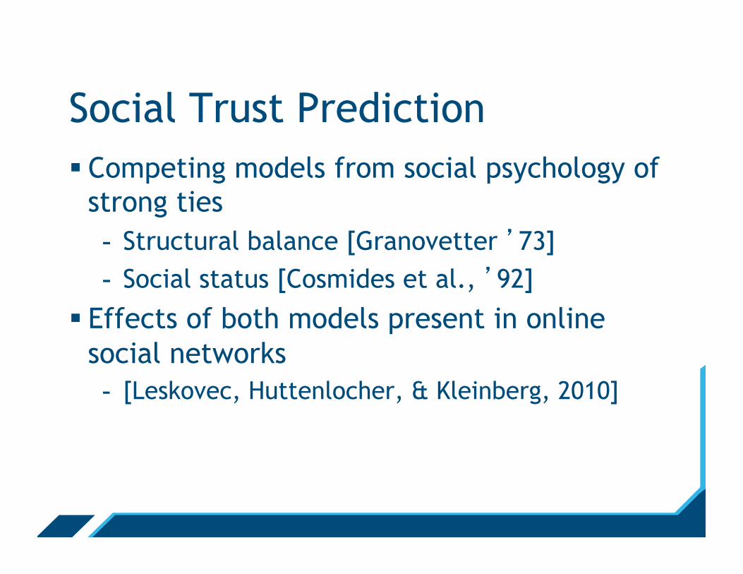
Social Trust Prediction § Competing models from social psychology of

strong ties -  Structural balance [Granovetter ’73] -  Social status [Cosmides et al., ’92]

§ Effects of both models present in online social networks

-  [Leskovec, Huttenlocher, & Kleinberg, 2010]

Structural Balance vs. Social Status"§  Structural balance: strong ties are governed

by tendency toward balanced triads"-  e.g., the enemy of my enemy..."

§  Social status: strong ties indicate unidirectional respect, “looking up to”, expertise status"-  e.g., patient-nurse-doctor, advisor-advisee"

2

–+–

+++

A

B

C A

B

C

(a) Structurally-balanced triads

++

–

A B C

(b) Consistent status links

Fig. 1. Implied structures according to competing theories of structural balance and status. Thepositive trust relationships from A to B and B to C imply opposite relationships from C to A inthe two models.

illustrates examples of such stable structures. If A strongly trusts B, and B stronglytrusts C, then triadic closure implies that A will likely trust C (and vice versa). On theother hand, if A does not trust B, B does not trust C, and C does not trust A, thisrepresents an unstable state that structural balance theory suggests should be less likelyto occur, as the theory prefers triads with one or three strong trust links.

A competing idea is that these social systems are governed by status or reputation.This is related to ideas from social psychology on reputation [4], where individuals aretrusted based on their expertise in a particular area. In a social status model, the notionof trust is that the trustee (i.e., the person being trusted) is of higher status than thetruster (i.e., the person who is trusting). Thus, under a status model, individuals existin a hierarchy from the most trustworthy to the least trustworthy, along which trustpropagates in triangular structures. As for structural balance, if A strongly trusts B, andB strongly trusts C, then status also implies that A will likely trust C. However, asillustrated in Figure 1(b), in contrast to structural balance, status predicts that C willlikely not trust A in this case. Similarly, if A does not trust B and B does not trust C,then status disagrees with structural balance and implies that A likely does not trust C.

1.1 Related Work

A large community of research focuses on computational modeling of social trust.Methods for analyzing trust include graph-based approaches [5,6,7], probabilistic mod-els [8,9,10], as well as other logic-based approaches [11]. These contributions tend tobe fixed computational models based on particular theories of trust, whereas in this pa-per, we propose PSL as a general tool that provides the flexibility to explore variousmodels without the need to adapt and redesign inference algorithms.

The foundations for many of these computational approaches stem from the vastsociological and psychological literature on human behavior. Recent studies have ana-lyzed some of these theories in the context of social media data, specifically comparingthe structural balance- and status-based models we emulate in this work [12,13]. Trust isalso an important topic in business analytics; for example, modeling of trust is a usefulcomponent for effective viral marketing and e-commerce [14].

2

–+–

+++

A

B

C A

B

C

(a) Structurally-balanced triads

++

–

A B C

(b) Consistent status links

Fig. 1. Implied structures according to competing theories of structural balance and status. Thepositive trust relationships from A to B and B to C imply opposite relationships from C to A inthe two models.

illustrates examples of such stable structures. If A strongly trusts B, and B stronglytrusts C, then triadic closure implies that A will likely trust C (and vice versa). On theother hand, if A does not trust B, B does not trust C, and C does not trust A, thisrepresents an unstable state that structural balance theory suggests should be less likelyto occur, as the theory prefers triads with one or three strong trust links.

A competing idea is that these social systems are governed by status or reputation.This is related to ideas from social psychology on reputation [4], where individuals aretrusted based on their expertise in a particular area. In a social status model, the notionof trust is that the trustee (i.e., the person being trusted) is of higher status than thetruster (i.e., the person who is trusting). Thus, under a status model, individuals existin a hierarchy from the most trustworthy to the least trustworthy, along which trustpropagates in triangular structures. As for structural balance, if A strongly trusts B, andB strongly trusts C, then status also implies that A will likely trust C. However, asillustrated in Figure 1(b), in contrast to structural balance, status predicts that C willlikely not trust A in this case. Similarly, if A does not trust B and B does not trust C,then status disagrees with structural balance and implies that A likely does not trust C.

1.1 Related Work

A large community of research focuses on computational modeling of social trust.Methods for analyzing trust include graph-based approaches [5,6,7], probabilistic mod-els [8,9,10], as well as other logic-based approaches [11]. These contributions tend tobe fixed computational models based on particular theories of trust, whereas in this pa-per, we propose PSL as a general tool that provides the flexibility to explore variousmodels without the need to adapt and redesign inference algorithms.

The foundations for many of these computational approaches stem from the vastsociological and psychological literature on human behavior. Recent studies have ana-lyzed some of these theories in the context of social media data, specifically comparingthe structural balance- and status-based models we emulate in this work [12,13]. Trust isalso an important topic in business analytics; for example, modeling of trust is a usefulcomponent for effective viral marketing and e-commerce [14].

Structural Balance in PSL

Knows(A,B) ^ Knows(B ,C ) ^ Knows(A,C )

^Trusts(A,B) ^ Trusts(B ,C ) ) Trusts(A,C ),

Tr(A,B) ^ Tr(B ,C ) ) Tr(A,C ),

Tr(A,B) ^ ¬Tr(B ,C ) ) ¬Tr(A,C ),

¬Tr(A,B) ^ Tr(B ,C ) ) ¬Tr(A,C ),

¬Tr(A,B) ^ ¬Tr(B ,C ) ) Tr(A,C )

[Huang, et al., SBP ‘13]

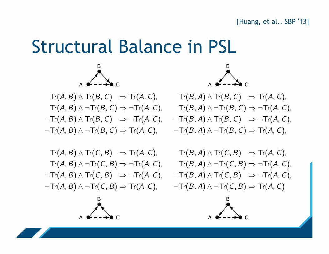
Structural Balance in PSL


Social Status in PSL


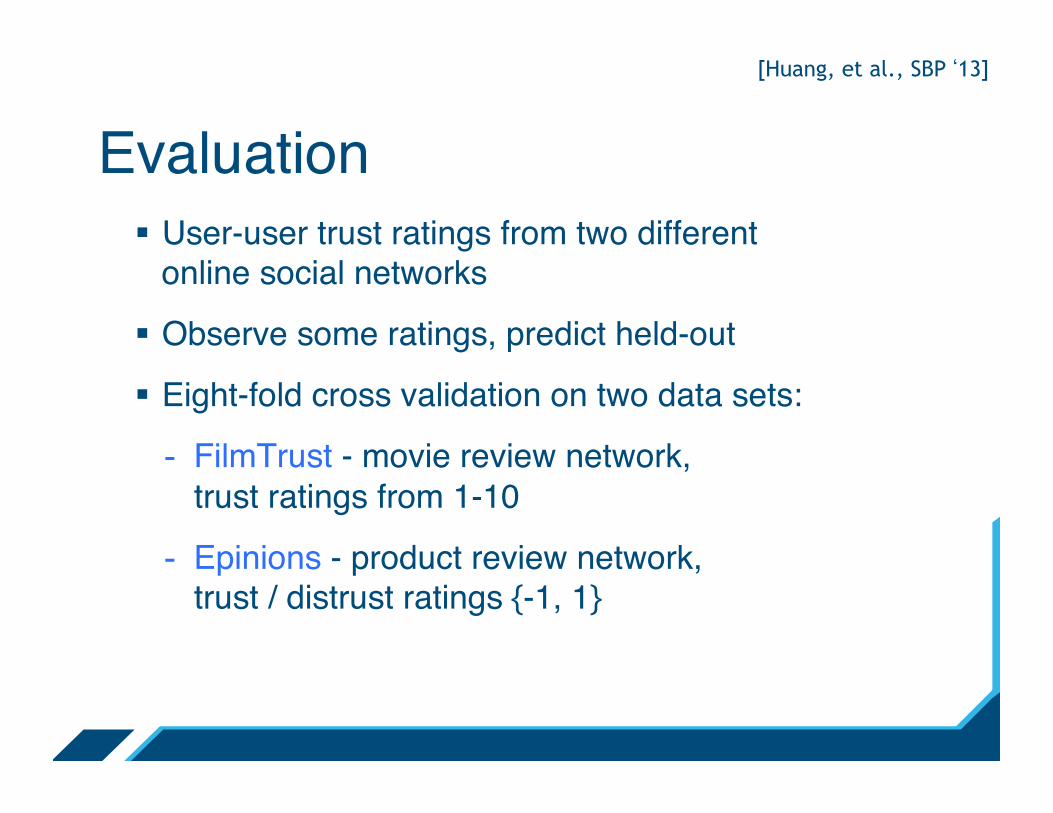
Evaluation"§  User-user trust ratings from two different

online social networks"

§ Observe some ratings, predict held-out"

§  Eight-fold cross validation on two data sets:"

-  FilmTrust - movie review network, trust ratings from 1-10"

-  Epinions - product review network, trust / distrust ratings {-1, 1}"


FilmTrust Experiment"§  Normalize [1,10] rating to [0,1]"§  Prune network to largest connected-component"§  1,754 users, 2,055 relationships"§  Compare mean average error, Spearman’s rank coefficient,

and Kendall-tau distance"

* measured on only non-default predictions"


Epinions Experiment"§  Snowball sample of 2,000 users from

Epinions data set "§  8,675 trust scores normalized to {0,1}"§ Measure area under precision-recall curve

for distrust edges (rarer class)"



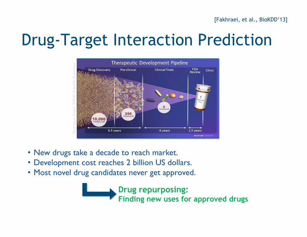
Drug-Target Interaction Prediction

Illus

trat

ion

Cre

dit:

XV

IVO

Sci

entifi

c A

nim

atio

n

• New drugs take a decade to reach market. • Development cost reaches 2 billion US dollars. • Most novel drug candidates never get approved.

[Fakhraei, et al., BioKDD’13]

Drug repurposing: Finding new uses for approved drugs


Drug-Target Interaction Prediction

Data: drug-target (gene product) interaction network + drug-drug and target-target similarities

Task: link prediction

Computational predictions focus biological investigations



Drug-Target Interaction Prediction [Fakhraei, et al., BioKDD’13]


Drug-Target Interaction Prediction •  315 Drugs, 250 Targets •  78,750 possible interactions, 1,306 observed interactions •  5 drug-drug similarities, 3 target-target similarities

Method AUROC Condition PSL 0.931 ± 0.018 10-fold CV Perlman, et al. 2011 0.935

with sampling Yamanishi, et al. 2008 0.884 Bleakley, et al. 2009 0.814


0

0.1

0.2

0.3

0.4

0.5

0.6

0 10 20 30 40 50 60 70 80 90 100

Prec

isio

n

Top N Predictions

with weight learning

without weight learning

Learning Latent Groups §  Can we better understand political discourse in social media by learning groups of similar people? §  Case study: 2012 Venezuelan Presidential Election §  Incumbent: Hugo Chávez §  Challenger: Henrique Capriles

Left: This photograph was produced by Agência Brasil, a public Brazilian news agency. This file is licensed under the Creative Commons Attribution 3.0 Brazil license. Right: This photograph was produced by Wilfredor. This file is licensed under the Creative Commons Attribution-Share Alike 3.0 Unported license.

[Bach, et al., ICML WS 2013]

Learning Latent Groups §  South American tweets collected from 48-hour window around election. §  Selected 20 top users §  Candidates, campaigns, media, and most retweeted

§  1,678 regular users interacted with at least one top user and used at least one hashtag in another tweet §  Those regular users had 8,784 interactions with non-top users

Learning Latent Groups

Schema Matching § Correspondences between

source and target schemas § Matching rules

-  ‘’If two concepts are the same, they should have similar subconcepts’’

-  ‘’If the domains of two attributes are similar, they may be the same’’

Organization

Customers Service & Products

provides

buys

Company

Customer Products & Services

develop

buys

Portfolios includes

develop(A, B) <= provides(A, B) Company(A) <= Organization(A)

Products&Services(B) <= Service&Products(B)

[Memory, Kimmig, Getoor, in prep]

Schema Mapping §  Input: Schema matches § Output: S-T query pairs (TGD)

for exchange or mediation § Mapping rules

-  “Every matched attribute should participate in some TGD.”

-  “The solutions to the queries in TGDs should be similar.”

Organization

Customers Service & Products

provides

buys

Company

Customer Products & Services

develop

buys

Portfolios includes

∃Portfolio P, develop(A, P) ∧ includes(P, B) <= provides(A, B) . . .

[Memory, Kimmig, Getoor, in prep]

Knowledge Graph Identification § Problem: Collectively reason about noisy,

inter-related fact extractions § Task: NELL fact-promotion (web-scale IE)

-  Millions of extractions, with entity ambiguity and confidence scores

-  Rich ontology: Domain, Range, Inverse, Mutex, Subsumption

§ Goal: Determine which facts to include in NELL’s knowledge base

Pujara, Miao, Getoor, Cohen, ISWC 2013

Knowledge Graph Identification

§  Performs graph identification: -  entity resolution -  collective classification -  link prediction

§  Enforces ontological constraints §  Incorporates multiple uncertain sources

Noisy extractions from the

Web

Joint reasoning Knowledge Graph

=

Problem:

Solution: Knowledge Graph Identification (KGI)


Graph Identification in KGI

𝑆𝐴𝑀𝐸𝐸𝑁𝑇(𝐸1, 𝐸2) ⋀. 𝐿𝐵𝐿(𝐸1, 𝐿) ⟹ 𝐿𝐵𝐿(𝐸2, 𝐿) 𝑆𝐴𝑀𝐸𝐸𝑁𝑇(𝐸1, 𝐸2) ⋀. 𝑅𝐸𝐿(𝐸1, 𝐸, 𝑅) ⟹ 𝑅𝐸𝐿(𝐸2, 𝐸, 𝑅) 𝑆𝐴𝑀𝐸𝐸𝑁𝑇(𝐸1, 𝐸2) ⋀. 𝑅𝐸𝐿(𝐸, 𝐸1, 𝑅) ⟹ 𝑅𝐸𝐿(𝐸, 𝐸2, 𝑅)

Noisy Extractions:

Entity Resolution:


KGI Representation of Ontological Rules

Adapted from Jiang et al., ICDM 2012

Illustra/on of KGI

Ontology: Dom(hasCapital, country) Mut(country, bird)

Extractions: Lbl(Kyrgyzstan, bird) Lbl(Kyrgyzstan, country) Lbl(Kyrgyz Republic, country)

Rel(Kyrgyz Republic, Bishkek, hasCapital)

Entity Resolution: SameEnt(Kyrgyz Republic,

Kyrgyzstan)

country

Kyrgyzstan Kyrgyz Republic

bird

Bishkek

SameEnt

Dom Lbl

Rel(h

asCap

ital)

Lbl Lbl

Kyrgyzstan

Kyrgyz Republic Bishkek country

Rel(hasCapital) Lbl

Representa1on as a noisy knowledge graph

A<er Knowledge Graph Iden1fica1on

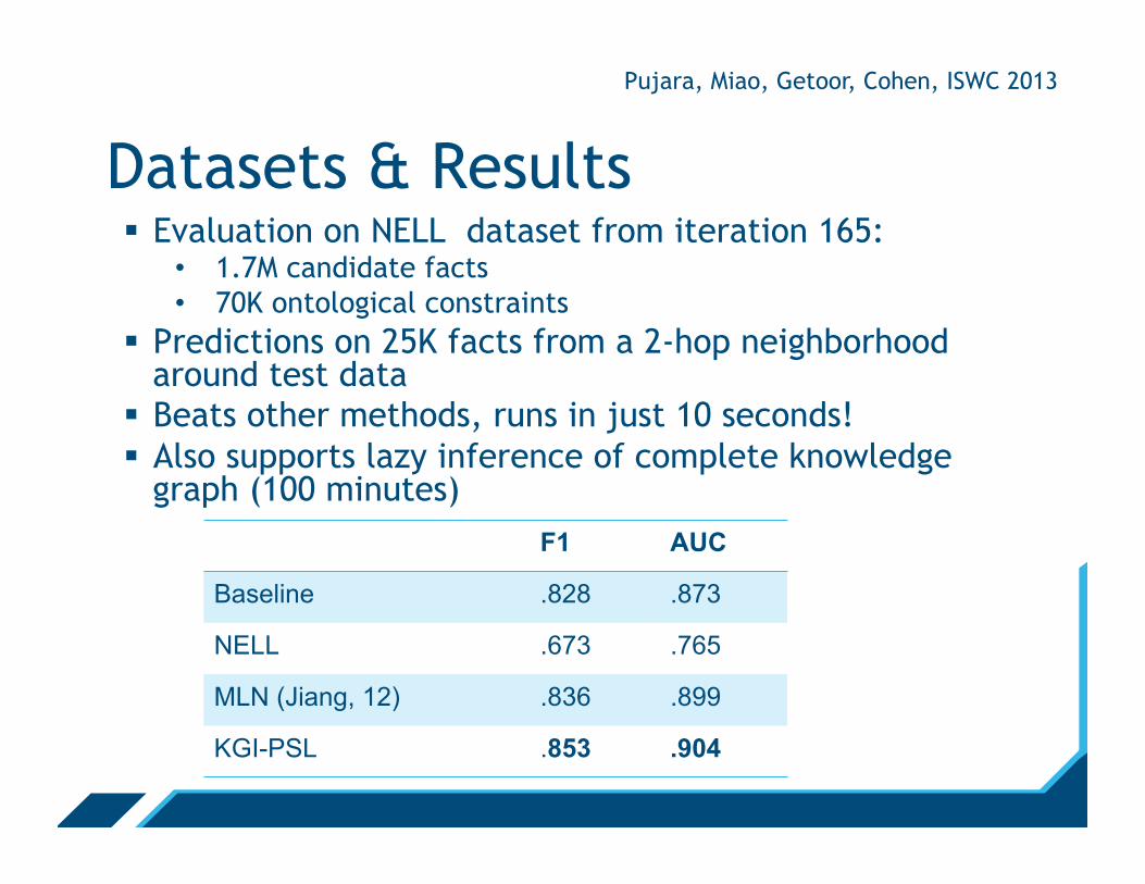
Datasets & Results §  Evaluation on NELL dataset from iteration 165:

•  1.7M candidate facts •  70K ontological constraints

§  Predictions on 25K facts from a 2-hop neighborhood around test data

§  Beats other methods, runs in just 10 seconds! §  Also supports lazy inference of complete knowledge

graph (100 minutes) F1 AUC

Baseline .828 .873

NELL .673 .765

MLN (Jiang, 12) .836 .899

KGI-PSL .853 .904



Conclusion


Closing Comments § Great opportunities to do good work and

do useful things in the current era of big data, information overload and network science – ‘entity-oriented data science’

§ Statistical relational learning provides some of the tools, much work still needed, developing theoretical bounds for relational learning, scalability, etc.

§ Compelling applications abound!

Looking for students & postdocs


psl.umiacs.umd.edu

entity-oriented data science - nist · · 2013-09-05" entity resolution – clustering nodes...

Documents