ENIQ 2nd Pilot Study

ENIQ Report nr. 28

EUR 22540 EN

Compilation of Modelling Resultsand Comparison with Inspection Data

DG JRCInstitute for Energy

2006

Editor: T. Seldis

Mission of the Institute for Energy The Institute for Energy provides scientific and technical support for the conception, development, implementation and monitoring of community policies related to energy. Special emphasis is given to the security of energy supply and to sustainable and safe energy production. European Commission Directorate-General Joint Research Centre (DG JRC) http://www.jrc.ec.europa.eu/ Institute for Energy, Petten (the Netherlands) http://ie.jrc.ec.europa.eu/ Contact details: Arne Eriksson Tel: +31 (0) 224 56 5383 E-mail: arne.eriksson@jrc.nl Legal Notice Neither the European Commission nor any person acting on behalf of the Commission is responsible for the use which might be made of this publication. The use of trademarks in this publication does not constitute an endorsement by the European Commission. The views expressed in this publication are the sole responsibility of the editor and do not necessarily reflect the views of the European Commission. A great deal of additional information on the European Union is available on the Internet. It can be accessed through the Europa server http://europa.eu/ EUR 22540 EN ISSN 1018-5593 Luxembourg: Office for Official Publications of the European Communities © European Communities, 2006 Reproduction is authorised provided the source is acknowledged. Printed in the Netherlands

European Commission Directorate General Joint Research Centre Institute for Energy Petten, The Netherlands

ENIQ 2nd PILOT STUDY

Compilation of Modelling Results And Comparison with Inspection Data

December 2006 ENIQ Report nr. 28 EUR 22540 EN

Approved by the Steering Committee of ENIQ for publication

Foreword The present work is one outcome of the activity of the ENIQ Task Group for Qualification (TGQ) on the ENIQ Second Pilot Study. ENIQ, the European Network for Inspection and Qualification, is driven by the nuclear utilities in the European Union and Switzerland and managed by the European Commission’s Joint Research Centre (JRC). It is active in the field of in-service inspection (ISI) of nuclear power plants by non-destructive testing (NDT), and works mainly in the areas of qualification of NDT systems and risk-informed in-service inspection (RI-ISI). This technical work is performed in two task groups: TG Qualification and TG Risk. A key achievement of ENIQ has been the issue of a European Qualification Methodology Document, which has been widely adopted across Europe. This document defines an approach to the qualification of inspection procedures, equipment and personnel based on a combination of technical justification (TJ) and test piece trials (open or blind). The TJ is a crucial element in the ENIQ approach, containing evidence justifying that the proposed inspection will meet its objectives in terms of defect detection and sizing capability. A Qualification Body reviews the TJ and the results of any test piece trials and it issues the qualification certificates. ENIQ has previously conducted a pilot study to assess the feasibility of the ENIQ Methodology in practice. This first pilot study was successful but, because the component chosen for the study was an austenitic weld, could not fully explore the use of TJs. This is because techniques such as mathematical modelling, at the time of the study, tended to be applicable only to isotropic materials. Assessment of the inspectability of austenitic welds usually requires the use of test pieces with the same metallurgical structure. Accordingly, ENIQ decided to conduct a second pilot study using a ferritic nozzle to shell weld. The main objective of the 2nd pilot study was to show how to fully exploit the potential of TJs in the qualification of inspection procedures and thereby reduce the number of test piece trials on full-scale components. As the subject of the study, a ferritic BWR-type nozzle to shell weld was selected. A TJ was produced, partly relying on modelling, to predict whether a designated ultrasonic inspection would be successful in detecting the specified defects. In parallel, a test piece with deliberately introduced defects was fabricated and inspected with the inspection system specified in the TJ. Predictions and inspection results were compared. In addition, as a separate exercise, three different mathematical models were used to predict the responses of the defects in the test piece to provide information on model applicability and accuracy of prediction. This report summarises the results of the modelling exercise. The contributors, in alphabetical order, are listed below. Special recognition should be given to several specific individuals listed below who made a particularly significant input into the commenting process.

1

I Atkinson Kande, United Kingdom J-A Berglund Ringhals NPP, Sweden R Booler Serco, United Kingdom, Chairman of Task Group Qualification since November 2005 R Chapman British Energy, United Kingdom D Couplet Tractebel, Belgium A Eriksson Directorate General JRC, European Commission L Horácek NRI- Řež, Czech Republic A Jonsson Forsmark NPP, Sweden P Kelsey Rolls-Royce Marine Power, United Kingdom P Krebs Engineer Consulting, Switzerland L Le Ber CEA – Saclay, France B Neundorf Vattenfall Europe Nuclear Energy, Germany T Seldis Directorate General JRC, European Commission, Co-chairman of TGQ H Söderstrand SQC Swedish NDT Qualification Centre, Sweden C Waites Serco, United Kingdom A Walker Rolls-Royce Marine Power, United Kingdom J Whittle John Whittle & Associates, United Kingdom, Chairman of TGQ until November 2005 H Wirdelius Chalmers University of Technology, Sweden The Steering Committee of ENIQ has formally approved this document for publication as an ENIQ report during the 30th SC meeting held in Helsinki (FIN) on 20-21 June 2006. The voting members of the Steering Committee of ENIQ are, in alphabetical order: R Chapman British Energy, United Kingdom, ENIQ Chairman P Daoust Tractebel, Belgium C Faidy EDF-Septen, France K Hukkanen Teollisuuden Voima OY, Finland P Krebs Engineer Consulting, Switzerland B Neundorf Vattenfall Europe Nuclear Energy, Germany, ENIQ Vice-Chairman J Neupauer Slovenské Elektrárne, Slovakia S Pérez Iberdrola, Spain U Sandberg Forsmark NPP, Sweden P Kopčil Dukovany NPP, Czech Republic D Szabó Paks NPP, Hungary European Commission representatives in the Steering Committee: A Eriksson Directorate General JRC, European Commission, ENIQ Network Manager T Seldis Directorate General JRC, European Commission, Scientific Secretary to ENIQ

2

CONTENT

1 Introduction 4 2 Scope of the work 4 3 Test piece 4 3.1 Type and dimensions 3.2 Type of implanted defects 5 4 Inspection 6 4.1 Technique and scan patterns 6 4.2 Probes 6 5 Modelling 6 5.1 Inspection from the inside of the unclad test piece 6 5.1.1 Assumptions 6 5.1.2 Defects to be modelled 7 5.1.3 Modelling results 8 5.1.2 Comparison with inspection results 10 5.2 Inspection from the outside of the clad test piece 12 5.2.1 Assumptions 12 5.2.2 Defects to be modelled 13 5.2.3 Modelling results 14 5.2.2 Comparison with inspection results 15 6 References 16

3

1 Introduction

This report is part of the ENIQ 2nd Pilot Study, concerned with the qualification of ultrasonic inspection of a Boiling Water Reactor (BWR) nozzle-to-shell weld, or more specifically, with the role of the technical justification within the inspection qualification process. This document compiles the results of the two modelling campaigns carried out in the ENIQ 2nd Pilot Study. A comparison between the theoretical predictions and real inspection data is reported as well. Note that the modelling work, which is described hereafter, is part of the 2nd ENIQ Pilot Study. However, this work has nothing to do with the qualification exercise itself. The work was done in parallel with the qualification to illustrate what modelling could do and identify its limitations. The inspection simulations described hereafter are exclusively carried out for the ENIQ 2nd Pilot Study.

2 Scope of the work

The scope of the work consisted of the two modelling campaigns and data from inspection of the component. Simulations and inspection covers detection by peak amplitude, but not sizing:

• Simulating the inspection from the inside of the unclad BWR test piece and predicting the peak amplitude values of a number of defect/probe combinations.

• Simulating the inspection from the outside of the clad BWR test piece and predicting

the peak amplitude values of a number of defect/probe combinations.

• Comparing the predicted and measured peak amplitude values. The defects considered are surface breaking cracks and lack-of-fusion defects, located in the weld and its heat affected zone (HAZ) in the inner 1/3 volume. The modelling has been carried out using three different models. The anonymity of the model is preserved, so that they are just referred to as model A, B, and C.

3 Test piece

3.1 Type and dimensions The test piece is a full-scale BWR nozzle component with a nozzle to shell weld. The nozzle and shell plates are made of ferritic steel equivalent to reactor pressure standards. The cladding at the inner surface is a 6-8 mm 2-layer strip cladding of austenitic steel. Figure 1 shows a sketch of the test piece and its main dimensions are given in Table 1.

4

Figure 1: Test piece.

Vessel diameter

[mm]

Inner radius[mm]

Weld prep. angle [deg]

Shell thickn. [mm]

Nozzle diam. [mm]

Shell weld diam. [mm]

Nozzle surface to shell weld centre

[mm]

~6400 95 4 160 270 700 215

Table 1: Main dimensions of the test piece. 3.2 Type of implanted defects Three different type of defects have been implanted in the test piece: i) surface breaking defects with crack tips both in the clad and base material, ii) near surface defects extending from the clad-base material interface inwards, iii) sidewall lack of fusion defects located at the weld preparation face. The first two types are PISC type A defects, whereas the latter is fabricated by the so-called coupon technique. All defects are positioned in the weld or in the associated heat affected zone. Defect orientation is parallel to the weld, with a tilt angle between 0º and 20º, and skew angle of 0º or 5º. For more details the reader is referred to reference 1.

5

4 Inspection

4.1 Technique and scan patterns The inspection technique applied for detection was ultrasonic contact technique, with water as couplant and the probes scanning perpendicular to the weld centre line. More details are given in references 1-3. 4.2 Probes The following probes – all with flat wedges – have been used for detection. The TRL probes have a focus depth of 8 and 12 mm respectively (F8 and F12).

Probe Wave mode Beam angle [º] Frequency [MHz] Crystal size [mm] T 45 Transversal 45 1.5 32x25 T 60 Transversal 60 1.5 32x21 T 70 Transversal 70 1.5 32x18

Tandem Transversal 45 1.5 32x25 TRL 70 F8 Longitudinal 70 2.0 2(25x15)

TRL 70 F12 Longitudinal 70 2.0 2(Ø 18)

Table 2: Probes used for detection.

5 Modelling

5.1 Inspection from the inside of the unclad test piece 5.1.1 Assumptions The specimen is assumed to be plane with parallel faces and isotropic material properties. The wall thickness is 160 mm. The contact probes are water-coupled. The pulse-echo and tandem configuration is shown in Figs. 2 and 3.

6

y

beam angle

height

tilteff

depth

nozzle Fig. 2: Pulse-echo configuration.

ynozzle

height

depth

tilteffbeam angle beam angle

160 mm

220 mm Fig. 3: Tandem configuration. 5.1.2 Defects to be modelled Table 3 gives an overview of the relevant defects for the simulation of the inside inspection of the unclad test piece. Defects 1, 8, 9, 10, 11, and 12 are surface breaking PISC type A defects. For more details on the implanted PISC type A defects the reader is referred to reference 1. Defects 13-17 are sidewall lack of fusion defect simulations utilising rectangular coupons.

7

defect azimuth [º] ligam. [mm] length [mm] height [mm] skew [º] tilt [º] tilteff [º] D01 13 0 20 5 0 0 1.4 D08 144 0 20 5 5 10 -6.3 D09 162 0 40 10 0 4 5.9 D10 186 0 40 10 5 20 20.7 D11 211 0 60 15 0 10 13.2 D12 238 0 60 15 5 0 5.3 D13 257 2 20 10 0 4 10.2 D14 278 12 30 15 0 4 2.2 D15 302 22 30 15 0 4 9.2 D16 324 2 50 5 0 4 -0.7 D17 350 7 60 5 0 4 5.1

Table 3: Defects to be modelled for the inside inspection. As already mentioned, the modelling treats the specimen as a flat plate, i.e. the defect tilt angles were adjusted to account for the change in effective tilt angle arising from the curvature of the test piece. More details of the implanted defects are given in reference 1. 5.1.3 Modelling results The Tables 4-6 show the peak amplitude values predicted respectively by model A, B, and C. The left column displays the defect number, the top row contains information about the probe type and the scanning direction. The letter “n” stands for scans with the probe beam axis pointing in negative y-direction (see Figs. 2-3) and “p” means positive. The abbreviations F8 and F12 refer to the depth of the focal points of the TRL probes, 8 mm and 12 mm respectively. The peak amplitude values are given in decibels relative to the response from reference reflectors. The reference reflectors are: Ø 3.2 mm SDH at 5 mm depth for the TRL 70 F8 probe, Ø 3.2 mm SDH DAC for the TRL 70 F12 probe, Ø 6.4 mm SDH DAC for the T 45, T 60, and T 70 probes, and Ø 8.0 mm SDH at 40 mm depth for tandem. In some cases, model A predicts amplitude values for both the top and the bottom defect edge. In Table 4 the letters “T” (top) and “B” (bottom) point out for which edge of the defect the given value is computed. The asterisk in Table 4 indicates that there is less confidence in the prediction, because the defect is located in the near-field zone of the interrogating probe. The simulations made with model B were executed with fixed frequency (centre frequency) in order to receive maximum amplitude within prescribed measuring mesh. By experience amplitude calculated with fixed frequency and that in time domain only differs 1-2 dB. The ultrasonic procedure specifies a time gating (it was developed for inspection of a component with cladding) and excludes all information within 10 mm from the probe. Since the inspection only picks up the diffracted signals from defects 1 and 9 it is not relevant to compare model B (monochromatic) and corresponding time gated information. These data are thus indicated in Table 5 with an asterisk.

8

defect TRL 70

F8, n TRL 70

F8, p TRL 70 F12, n

TRL 70F12, p

T 45 n

T 45 p

T 60 n

T 60 p

T 70 n

T 70 p

Tandemn

D01 D08 D09 D10

D11 T D11 B -7.9* -3.0* D12 T D12 B -4.3* -3.3* D13 T D13 B -14.1* -10.1 D14 T -23.5* -17.3 D14 B -10.9* -7.8 -2.0* D15 T -25.7* -21.2 D15 B -13.2 -9.5 -1.6* D16

D17 T D17 B -12.2* -8.7

Table 4: Peak amplitude values (dB) predicted by model A. *) Value with less confidence.

defect TRL 70

F8, n TRL 70

F8, p TRL 70 F12, n

TRL 70F12, p

T 45 n

T 45 p

T 60 n

T 60 p

T 70 n

T 70 p

Tandemn

D01 -22.0* 29.2* 32.3* -0.2* D08 D09 26.6* 22.0* 24.7* 21.0* D10 D11 D12 D13 16.1 10.9 13.5 14.1 D14 8.6 8.8 6.1 14.5 D15 -2.5 6.5 7.4 14.0 D16 D17

Table 5: Peak amplitude values (dB) predicted by model B. *) Value with less confidence.

9

defect TRL 70

F8, n TRL 70

F8, p TRL 70 F12, n

TRL 70F12, p

T 45 n

T 45 p

T 60 n

T 60 p

T 70 n

T 70 p

Tandemn

D01 D08 D09 14.0* -12.8* -8.3* D10 -15.1* -13.6* -12.8* D11 -14.8* -13.6 -12.7* D12 -14.3* -13.3* -8.3* D13 -8.0 9.5 -10.7 6.3 -20.1* -19.0* -15.6* -13.5 D14 -7.4 -6.9 -4.5 -19.6* -14.7 -12.7 -12.1 -9.7 -5.2 D15 -3.7 -19.9* -18.6* -9.1 -15.1 -4.3 -5.5 D16 2.9 0.8 -0.9 -2.4 -18.9* -13.9* -8.7* -23.4 D17 -1.7 -1.3 -5.2 -0.2 -19.4* -17.9* -13.4* -14.6

Table 6: Peak amplitude values (dB) predicted by model C. *) Value with less confidence. The asterisk in Table 6 points out cases in which a rougher discretisation of the defect surface was chosen for model C. Note that the predictions of model C for both TRL probes and the tandem configuration have been computed after the release of the inspection data. 5.1.4 Comparison with inspection results Table 7 shows the measured peak amplitude values obtained after the unclad test piece has been inspected from the inside. The values are given in decibels relative to the response from reference reflectors. The reference reflectors are identical with those described in Section 5.1.3. The abbreviations and letters used in Table 7 are the same as in Tables 4-6.

defect TRL 70

F8, n TRL 70

F8, p TRL 70 F12, n

TRL 70F12, p

T 45 n

T 45 p

T 60 n

T 60 p

T 70 n

T 70 p

Tandemn

D01 -4.6 -6.9 -6.7 -6.7 -12.5 D08 4.2 0.5 -13.5 D09 -6.7 -1.0 -10.8 -2.9 -8.0 D10 -13.5 3.8 -15.8 2.7 D11 -8.0 0.8 -9.8 -1.3 -12.0 D12 -4.4 -3.2 -7.2 -4.8 -6.7 D13 -11.6 6.2 -8.5 5.1 -5.2 D14 -4.8 -11.2 -1.2 -9.4 -8.8 -3.2 0.2 2.9 D15 -3.4 -9.1 -5.8 3.5 6.5 D16 -5.0 -6.5 -5.0 -5.2 -1.8 D17 -4.3 -3.4 -5.8 1.0 0.4

Table 7: Peak amplitude values (dB) obtained after inside inspection of the unclad test piece.

10

A comparison between the predicted peak amplitude values and the measured peak amplitude values has been carried out, and the results are shown in Tables 8-10. The difference of the predicted peak amplitude value with regard to the measured peak amplitude value has been calculated. The values are given in decibels relative to the response from reference reflectors. Note that for model A only the predictions for the bottom edge of defect 14 and 15 have been compared with the inspection result, because the amplitudes are much stronger than the ones from the top edge.

defect TRL 70

F8, n TRL 70

F8, p TRL 70 F12, n

TRL 70F12, p

T 45 n

T 45 p

T 60 n

T 60 p

T 70 n

T 70 p

Tandemn

D01 D08 D09 D10 D11 D12 D13 D14 -1.5* -4.6 -4.9* D15 -3.7 -8.1* D16 D17

Table 8: Difference (dB) of the peak amplitude value predicted by model A with regard to

the measured value. *) Value with less confidence.

defect TRL 70

F8, n TRL 70

F8, p TRL 70 F12, n

TRL 70F12, p

T 45 n

T 45 p

T 60 n

T 60 p

T 70 n

T 70 p

Tandemn

D01 12.3* D08 D09 29.0* D10 D11 D12 D13 19.3 D14 18.2 9.3 11.6 D15 13.2 7.5 D16 D17

Table 9: Difference (dB) of the peak amplitude value predicted by model B with regard to

the measured value. *) Value with less confidence.

11

defect TRL 70

F8, n TRL 70

F8, p TRL 70 F12, n

TRL 70F12, p

T 45 n

T 45 p

T 60 n

T 60 p

T 70 n

T 70 p

Tandemn

D01 D08 D09 D10 D11 D12 D13 3.6 3.3 -2.2 1.2 -8.3 D14 -2.6 4.3 -3.3 -5.3 -3.9 -8.9 -9.9 -8.1 D15 -0.3 0.0 -9.3 -7.8 -12.0 D16 7.9 7.3 4.1 2.8 -21.6 D17 2.6 2.1 0.6 -1.2 -15.0

Table 10: Difference (dB) of the peak amplitude value predicted by model C with regard to

the measured value. 5.2 Inspection from the outside of the clad test piece 5.2.1 Assumptions The specimen is assumed to be plane with parallel faces. Both the base material and the cladding are assumed to be isotropic. The attenuation in the cladding and any reflections at the interface between the clad layer and the base material is not taken into account. During the inspection it was revealed that 6dB was a proper amplification to compensate for transfer losses. Some of the models can model this (viscous damping) but the information was not provided to the modellers. The wall thickness of the specimen is 168 mm. The contact probes are water-coupled. The pulse-echo and tandem configuration is shown in Figs. 4 and 5.

y

beam angle

height

tilteff

depth

nozzle Fig. 4: Pulse-echo configuration.

12

ynozzle

height

depth

tilteffbeam angle beam angle

168 mm

220 mm Fig. 5: Tandem configuration. 5.2.2 Defects to be modelled Table 11 gives an overview of the relevant defects for the simulation of the outside inspection of the clad test piece. Defects 9-12 are near surface PISC type A defects located under the clad. Defects 13-17 are sidewall lack of fusion defect simulations utilising rectangular coupons. defect azimuth [º] ligam. [mm] length [mm] height [mm] skew [º] tilt [º] tilteff [º] D09 162 150.1 40 10 0 4 -5.9 D10 186 150.6 40 10 5 20 -20.7 D11 211 145.4 60 15 0 10 -13.2 D12 238 145.1 60 15 5 0 -5.3 D13 257 147.2 20 10 0 4 -10.2 D14 278 132.0 30 15 0 4 -2.2 D15 302 122.5 30 15 0 4 -9.2 D16 324 152.0 50 5 0 4 0.7 D17 350 147.0 60 5 0 4 -5.1

Table 11: Defects to be modelled for the outside inspection. The defect tilt angles were adjusted to account for the change in effective tilt angle arising from the curvature of the test piece.

13

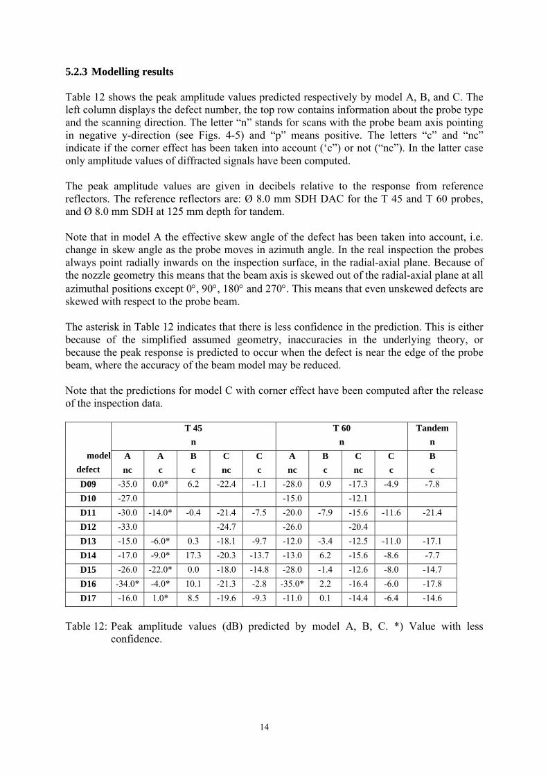
5.2.3 Modelling results Table 12 shows the peak amplitude values predicted respectively by model A, B, and C. The left column displays the defect number, the top row contains information about the probe type and the scanning direction. The letter “n” stands for scans with the probe beam axis pointing in negative y-direction (see Figs. 4-5) and “p” means positive. The letters “c” and “nc” indicate if the corner effect has been taken into account (‘c”) or not (“nc”). In the latter case only amplitude values of diffracted signals have been computed. The peak amplitude values are given in decibels relative to the response from reference reflectors. The reference reflectors are: Ø 8.0 mm SDH DAC for the T 45 and T 60 probes, and Ø 8.0 mm SDH at 125 mm depth for tandem. Note that in model A the effective skew angle of the defect has been taken into account, i.e. change in skew angle as the probe moves in azimuth angle. In the real inspection the probes always point radially inwards on the inspection surface, in the radial-axial plane. Because of the nozzle geometry this means that the beam axis is skewed out of the radial-axial plane at all azimuthal positions except 0°, 90°, 180° and 270°. This means that even unskewed defects are skewed with respect to the probe beam. The asterisk in Table 12 indicates that there is less confidence in the prediction. This is either because of the simplified assumed geometry, inaccuracies in the underlying theory, or because the peak response is predicted to occur when the defect is near the edge of the probe beam, where the accuracy of the beam model may be reduced. Note that the predictions for model C with corner effect have been computed after the release of the inspection data.

T 45 n

T 60 n

Tandem n

model

defect A nc

A c

B c

C nc

C c

A nc

B c

C nc

C c

B c

D09 -35.0 0.0* 6.2 -22.4 -1.1 -28.0 0.9 -17.3 -4.9 -7.8 D10 -27.0 -15.0 -12.1 D11 -30.0 -14.0* -0.4 -21.4 -7.5 -20.0 -7.9 -15.6 -11.6 -21.4 D12 -33.0 -24.7 -26.0 -20.4 D13 -15.0 -6.0* 0.3 -18.1 -9.7 -12.0 -3.4 -12.5 -11.0 -17.1 D14 -17.0 -9.0* 17.3 -20.3 -13.7 -13.0 6.2 -15.6 -8.6 -7.7 D15 -26.0 -22.0* 0.0 -18.0 -14.8 -28.0 -1.4 -12.6 -8.0 -14.7 D16 -34.0* -4.0* 10.1 -21.3 -2.8 -35.0* 2.2 -16.4 -6.0 -17.8 D17 -16.0 1.0* 8.5 -19.6 -9.3 -11.0 0.1 -14.4 -6.4 -14.6

Table 12: Peak amplitude values (dB) predicted by model A, B, C. *) Value with less

confidence.

14

5.2.4 Comparison with inspection results Table 13 shows the measured peak amplitude values obtained after the clad test piece has been inspected from the outside. The values are given in decibels relative to the response from reference reflectors. The reference reflectors are identical with those described in Section 5.2.3. The abbreviations and letters used in Table 13 are the same as in Table 12.

T 45 n

T 60 n

Tandem n

defect Measurement

c Measurement

c Measurement

c D09 -1.9 -8.3 -5.3 D10 -6.9 -4.0 D11 0.5 -7.8 -5.4 D12 -3.6 -7.3 -0.8 D13 -6.4 -7.3 5.3 D14 -7.5 -7.1 6.8 D15 -9.2 -7.9 -7.5 D16 4.7 -5.6 0.4 D17 3.3 -5.2 6.7

Table 13: Peak amplitude values (dB) obtained after outside inspection of the clad test piece. A comparison between the predicted peak amplitude values and the measured peak amplitude values has been carried out, and the results are shown in Table 14. The difference of the predicted peak amplitude value with regard to the measured peak amplitude value has been calculated. The values are given in decibels relative to the response from reference reflectors.

T 45 n

T 60 n

Tandem n

model

defect A nc

A c

B c

C nc

C c

A nc

B c

C nc

C c

B c

D09 -33.1 1.9* 8.1 -20.5 0.8 -19.7 9.2 -9.0 3.4 -2.5 D10 -8.1 -5.2 D11 -30.5 -14.5* -0.9 -21.9 -8.0 -12.2 -0.1 -7.8 -3.8 -16.0 D12 -29.4 -21.1 -18.7 -13.1 D13 -8.6 0.4* 6.7 -11.7 -3.3 -4.7 3.9 -5.2 -3.7 -22.4 D14 -9.5 -1.5* 24.8 -12.8 -6.2 -5.9 13.3 -8.5 -1.5 -14.5 D15 -16.8 -12.8* 9.2 -8.8 -5.6 -20.1 6.5 -4.7 -0.1 -7.2 D16 -38.7* -8.7* 5.4 -26.0 -7.5 -29.4* 7.8 -10.8 -0.4 -18.2 D17 -19.3 -2.3* 5.2 -22.9 -12.6 -5.8 5.3 -9.2 -1.2 -21.3

Table 14: Difference (dB) of the peak amplitude value predicted by model A, B, C with

regard to the measured value. *) Value with less confidence.

15

6 References

1. ‘ENIQ 2nd Pilot Study – Modelling of Defects in ENIQ Nozzle Assembly 21 – Input Data’, ENIQ.TGQ(02) Input Data. Internal working document.

2. ‘Inspection Procedure for the 2nd ENIQ Pilot Study’, ENIQ Report ENIQ.PILOT2 (04)

4, March 2004. 3. ‘Inspection Procedure for the 2nd ENIQ Pilot Study – External Surface Inspection’,

ENIQ Report ENIQ.PILOT2 (05) 1, March 2005.

16

European Commission EUR 22540 EN – DG JRC – Institute for Energy ENIQ 2nd Pilot Study - Compilation of Modelling Results and Comparison with Inspection Data Editor Thomas Seldis Luxembourg: Office for Official Publications of the European Communities 2006 – 16 pp. – 21 x 29.7 cm EUR - Scientific and Technical Research Series; ISSN 1018-5593 Abstract The present report compiles the results of the mathematical modelling work carried out in the ENIQ 2nd Pilot Study. As the subject of the study a ferritic BWR-type nozzle to shell weld with deliberately introduced defects was selected. Three different models have been applied to predict the peak amplitude responses of the defects for two different ultrasonic inspection scenarios: i) inspection of the unclad BWR test piece from the inside and ii) inspection of the clad BWR test piece form the outside. The results of the simulations are reported and compared with real inspection data.

The mission of the Joint Research Centre is to provide customer-driven scientific and technical support for the conception, development, implementation and monitoring of EU policies. As a service of the European Commission, the JRC functions as a reference centre of science and technology for the Union. Close to the policy-making process, it serves the common interest of the Member States, while being independent of special interests, whether private or national.