enhancing sliding mode control with proportional...
TRANSCRIPT

Turk J Elec Eng & Comp Sci
(2015) 23: 126 – 148
c⃝ TUBITAK
doi:10.3906/elk-1301-182
Turkish Journal of Electrical Engineering & Computer Sciences
http :// journa l s . tub i tak .gov . t r/e lektr ik/
Research Article
Enhancing sliding mode control with proportional feedback and feedforward: an
experimental investigation on speed sensorless control of PM DC motor drives
Mehmet DAL∗
Department of Electricity and Energy, Kocaeli Vocational High School, Kocaeli University, Kocaeli, Turkey
Received: 24.01.2013 • Accepted: 19.03.2013 • Published Online: 12.01.2015 • Printed: 09.02.2015
Abstract:This paper investigates the enhancement of sliding mode control (SMC) with the combined use of feedforward
torque compensation and proportional error feedback control. The proposed enhancement is adapted to the control of
permanent magnet (PM) DC motor drives by synthesis of the equivalent control equation augmented as proportional
feedback and feedforward terms. A novel sliding function, introduced by utilizing the estimated load torque and
the estimated rotor current, is examined and compared with another known sliding function obtained by nonideal
differentiation of the estimated rotor speed. The significance of the proposed enhancements to SMC consists of the
elimination of disturbance, the reduction of the discontinuous control gain magnitude, and the reduction of chattering.
The contribution of this study is demonstrated by a performance comparison between several control versions, where
the aim is the achievement of good performances in both the speed estimation and state tracking accuracy in the speed
sensorless control of PM DC motor drives under varying load inertia. These latter statements are verified by several
comparative simulations and experiments.
Key words: Sliding mode control, chattering reduction, sensorless speed control, DC motor drives
1. Introduction
Modern control strategies have prompted the use of the permanent magnet (PM) DC motor as the most
efficient and economical actuator for high-performance motion control applications, including guided vehicles,
factory automation, robotics, and milling. In these applications, precise position and speed/torque controls
are required to perform the required tasks. The bandwidth of the closed loop varies linearly with the load
inertia. Therefore, linear controllers, like a fixed-gain proportional plus integral (PI) controller, cannot keep
the stability of the closed loop in the case of large inertia variations. However, linear controllers with improved
versions are confirmed as the state-of-the-art and most trustable controllers; thus, these controllers have the
most widespread applications in industry. Moreover, it has been verified that a combined use of feedforward
plus feedback with a linear controller can significantly improve performance in motion control systems, where
the feedforward term can eliminate the measurable disturbance effects that arise on the system output [1].
On the other hand, the sliding mode control (SMC) considered in variable structure control is a widely
known nonlinear, high-frequency switching feedback control approach. The main advantage of SMC consists
of robustness to bounded plant parameter variations and external disturbances, as well, as the fact that SMC
has an order reduction property that provides good dynamic response comparable to the behavior of first-order
systems [2–4]. In the past decade, therefore, the sliding mode approach has increasingly found a place in the
∗Correspondence: [email protected]
126

DAL/Turk J Elec Eng & Comp Sci
control of electric motor drives and power converters [5–7] and in many other applications, such as automotive
and flight controls, robotics, space devices, and the control of chemical process [8]. However, undesired high-
frequency oscillations on the system output that are caused by both high-magnitude control gain and nonideal
switching action are the main obstacle in the implementation of SMC. This phenomenon, which is known as
chattering, can, for example, wear out the mechanical actuators and increase the current ripple in the electrical
system. Furthermore, chattering may also lead to instability in closed-loop control systems [9].
Consequently, for the variable structure systems control community, the challenge has arisen to smooth
the discontinuous control and reduce the chattering while preserving the main properties of the SMC [10–12].
Reducing the switching control gain directly and/or using a smoothing filter are well-known methods that
result in the weakening of the sliding mode and unsatisfactory control performance [13]. A significant number
of studies proposed to smooth the discontinuous control were surveyed in [14] and the references therein, where
the main concern was to achieve an optimal trade-off between the tracking precision and control bandwidth.
However, these solutions are mostly theoretical, and the practical aspect of SMC is not considered much.
This paper aims to combine the advantages of the sliding mode approach with the feedforward torque
compensation plus a proportional error feedback to improve the control accuracy and robustness. The proposed
combined SMC law is derived by an alternative interpretation of the sliding mode equivalent control equation.
The feedforward component combines back-electromotive force (EMF) and the disturbance that arises in the
variation of load torque and mechanical parameters. The feedback signal includes the sum of the direct switching
SMC plus the proportional error feedback signal. A well-known combined (or integrated) speed control strategy
of DC motor drives proposed in [10] is considered as an adequate example to explore the properties of the
proposed enhancement to SMC, and its performance is assessed in the operation of a motor drive system under
2 different load inertia. Moreover, a novel switching function, formed using the estimated acceleration, is also
examined and compared with another switching function that uses nonideal differentiation of the estimated
angular speed. The estimated speed is obtained using a unified sliding mode observer proposed in [10] and the
load torque is estimated by the well-known disturbance observer proposed in [15].
The proposed combined SMC has several advantages: rejection of the disturbances that arise in the closed-
loop path, considerable reduction of the control gain magnitude, better trajectory tracking in both the transient
and steady-state conditions, cancellation of the filtering of the discontinuous control, and the minimization of
chattering. These statements are verified by comparative simulations and experiments, which are carried out
on a small-sized PM DC motor drive system. The hardware setup uses the recent rapid development of digital
signal processor (DSP)-based rapid control prototyping (RCP) tools [16], which make it easy to implement the
advanced control strategies without hand code writing.
2. Problem statement
The sliding mode equivalent control is a well-known approach found by recognizing that σ(x) = 0 is the necessary
condition to make the state trajectory stay on the sliding surface, σ(x) = 0 [2]. The SMC design is completed
in 2 steps by selecting a constructible switching function σ(x) and by synthesizing an adequate control law that
can force the system state to reach the sliding surface in a finite time and maintain it there forever. However,
the most distinguished ideal features of the SMC can arise when the frequency of the switching control is high,
theoretically infinite. However, imperfections in the switching action limits the switching frequency and causes
a nonideal sliding motion, where the trajectory remains close to the switching surface σ(x) = 0. The switching
function is the main factor in the formation of the discontinuous control, which naturally changes depending
127

DAL/Turk J Elec Eng & Comp Sci
on the sign of this function. Therefore, the system dynamics under sliding mode are governed by the switching
function σ(x) and thus by the desired control law, which has to be designed such that the desired dynamics are
obtained during sliding mode. A brief presentation of the equivalent control is provided in the following text.
Consider a system defined by x = Ax(t) + B(x)u ; inserting this equation into the differentiation of the
switching function σ(x) yields:
dσ(x)
dt= Gx = GAx(t) +GB(x)u, (1)
where the gradient matrix G = ∂σ∂x corresponds to the slope of the selected sliding surface. In Eq. (1), the
control that makes σ(x) = 0 is called the equivalent control, and by replacing u with ueq , it can be calculated
from Eq. (1) as:
ueq = − (GB)−1
GAx(t), (2)
which is not such a control actually applied to the system input, but is rather an interpretation of a control
that maintains a sliding motion on the sliding surface σ(x) = 0 [8]. A conventional direct switching form of
SMC is usually given by:
u(t) = −Msign(σ(t)), (3)
where M is the control gain, being a nonzero scalar, and sign is well-known sign function defined as sign(σ(t)) =
1 for σ(x) > 0 and u = ueq +Msgn(σ2) for σ(x) < 0.
The exact calculation of the equivalent control as given in Eq. (2) is possible if 2 constraints are satisfied,
i.e. the matrix GB has to be invertible, and there must be no disturbance and no parameter variations in
the controlled plant. Considering that most real systems have varying parameters, it is assumed that the
equivalent control can be captured by passing the discontinuous control in Eq. (3) through a low-pass filter
(LPF), i.e. T ˙ueq(t) + ueq(t) = u(t) [2], where ueq is the average value or estimation of the ideal continuous
control corresponding to the equivalent control given in Eq. (2), and T is the time constant of the LPF used
to capture the equivalent control. This approximation can be construed based on the fact that the equivalent
control has to be naturally continuous and corresponds to the low-frequency component of the switching control
given in Eq. (3). This construing can also be verified as inserting Eq. (2) into Eq. (1) implies the following:
σ(x) = −GB(x)(u− ueq). (4)
If the sliding mode exits once, i.e. σ(x) = 0 and σ(x) = 0, then the equivalent control becomes equal to the
actual control u , and the sliding motion will be maintained on the sliding surface σ(x) = 0. However, with
the use of the control in Eq. (3), a high magnitude of control gain is required to push the system state towards
the sliding surface and start the desired sliding motion. Unfortunately, not only is the increase of the gain
magnitude alone not enough to start a sliding motion, but it also increases the chattering magnitude. As stated
previously, reducing the control gain directly or passing the discontinuous control in Eq. (3) through a LPF
adversely affects the sliding mode existence. Based on this fact, a fast switching control signal passing through
a LPF may exhibit the same behavior as a SMC with a boundary layer using a saturation function [17].
On the other hand, in the case of DC motor drives with an H-bridge converter, a continuous control input
is required for pulse-width modulation (PWM) signal generation. Therefore, the control law in Eq. (3) has
to be passed through a LPF, but in this case, it provides an unsatisfactory tracking performance in the speed
128
DAL/Turk J Elec Eng & Comp Sci
sensorless control of DC motor drives [18]. This finding necessitates enhancing the SMC law in Eq. (3) in an
acceptable manner without losing its main properties.
Many strategies using SMC were proposed in order to improve the control performance and robustness to
external disturbances and plant parameter variations for DC motor drives in [19–21] and the references therein.
A recent method relevant to the high-order (second-order) SMC approach and proposed for the cascaded control
structure of DC motor drives was extensively studied in [22] and the references therein. The disadvantage of this
method is the requirement of a high-resolution speed feedback device, which is expensive. In order to reduce
the chattering, 2 different gain adaptation techniques proposed in [11] were adapted to current-controlled DC
motor drives in [23].
These adaptation techniques, however, were found to be unusable for the combined speed control of DC
motor drives in this present study. Consequently, the present paper investigates the further enhancement of
SMC with a reasonable assumption, where a combined SMC law is derived by an alternative interpretation of
the equivalent control for speed sensorless control of PM DC motor drives.
3. Proposed speed controller
3.1. Plant model
The dynamic model of a PM DC motor can be described by the following well-known equations:
di
dt= −R
Li− ke
Lω +
1
Lu, (5a)
dω
dt= −B
Jω +
1
Jkti−
1
JtL, (5b)
where u is the motor supply voltage; i is the rotor current; ω is the rotor angular speed; tL is the load torque;
R and L are the resistance and inductance of the rotor winding, respectively; ke and kt are the back-EMF
constant and motor torque constant, respectively; B is the viscous friction coefficient, which is usually neglected
to simplify the model; and J(= Ja + JL) is the combined inertia of the rotor and load.
3.2. Switching function
A linear combination between the tracking error of the angular velocity and its derivative is a suitable and usual
selection as the switching function for DC servo drive systems.
σ1 = c(ω∗ − ω) + (ω∗ − ω) (6)
Here, eω(= ω∗−ω) and eω(= ω∗− ω) denote the speed tracking error and its differentiation, respectively. From
a theoretical point of view, if the sliding mode exists, i.e. σ1(t) = 0 and σ1(t) = 0, on the switching surface in
Eq. (6), then the asymptotic convergence of the state error (eω(t) = eω(0)e−t/c) is guaranteed. On the other
hand, considering the existence of the sliding mode c(ω∗ − ω) + (ω∗ − ω) = 0 implies the rotor current to be:
i =J
kt(c(ω∗ − ω) + ω∗ +
1
JtL), (7)
which can be derived by inserting the acceleration in Eq. (5b) into Eq. (6), where the machine parameter B
is neglected. This finding verifies that the switching function in Eq. (6) enables one to establish a combined
129

DAL/Turk J Elec Eng & Comp Sci
speed/current control scheme for a DC motor, which is different than the conventional cascaded speed/current
control schemes. Moreover, if the existence of sliding mode is guaranteed with the use of Eq. (6), then, at least
theoretically, the drive system response becomes dependent on design parameter c only; thus, the controller
robustness with respect to parameter variations in the electrical and mechanical subsystem will be improved.
In this idea as suggested in [10], however, several practical issues should be considered in the implementation,
e.g., the control law in Eq. (3) is unsatisfactory to push the system state towards the sliding surface; thus,
an improved control law is required in the implementation [18]. On the other hand, the acceleration signal is
required to establish the switching function in Eq. (6), and it is difficult to get it precisely from the direct
measurement of the rotor angular speed due to the well-known exact differentiation problem [22]. In digital
controlled systems, therefore, the acceleration of the rotor shaft can normally be calculated by nonideal numeric
differentiation of the measured angular speed, which can be handled by an incremental encoder, or, alternatively,
it can be calculated by a state observer. The angular speed measured by an optical encoder is usually passed
through a LPF to suppress the undesired measurement noises, and then a nonideal differentiation can be
performed by digital controllers.
In order to improve the control performance of DC motor drives, the modified control version proposed
in [18] was given by u = M sign(sω)+Gpeω + ktω), where adding a proportional error feedback term arbitrary
to the switching control together with the back-EMF provides better speed tracking performance with respect
to both control laws, i.e. the conventional SMC in Eq. (3) and the well-known PI-based cascaded speed/current
control. However, with the use of the conventional SMC in Eq. (3), the rotor current ripple is mandatorily
acceptable. A further improvement of this control version is proposed in this study, which will be presented in
the next section.
3.3. Combined speed controller
A combined speed control strategy, suggested in [10], is considered for a further improved speed sensorless
control of DC motor drive in this study. The speed tracking error and its derivative are evaluated as the state
variables ω∗ − ω = eω = x1 and ω∗ − ω = eω = x2 , and then a linear combination between the angular speed
tracking error and its derivative is defined as the desired switching surface for the drive system.
σ1 = cx1 + x2 (8)
A controllable canonical state space model, which describes the tracking error dynamics in the closed-loop speed
control system, is given by:
x1 = x2 = ω∗ − ω, (9)
x2 = ω∗ − ω, (10)
and using Eqs. (5a), (5b), and (7), Eq. (10) is derived as follows:
x2 = −ktkeJL
cx1 −R
Lx2 + f(t)− kt
JLu, (11)
where f(t) = ω∗ + RL ω
∗ + RJL tL + ktke
JL ω∗ + kt
J tL is imposed as the disturbance entering the closed-loop control
path. In [10], the disturbance f(t) is disregarded, expecting that it will be compensated by discontinuous control
u = M sign(σ). However, it is a well-known fact that in real-life systems that operate under SMC, neglected
dynamics in the closed loop may result in chattering, which was experimentally verified in [18]. Based on this
130

DAL/Turk J Elec Eng & Comp Sci
finding, a further enhancement to SMC is aimed at in this paper considering an alternative interpretation of
Eq. (11). First, inserting Eq. (5a) into Eq. (10) yields
x2 = ω∗ − ktJi+
ktJtL, (12)
and inserting Eq. (5a) into Eq. (12) and then inserting Eq. (7) into the resulting equation gives
x2 = ω∗ − ktR
JL
J
kt
(c(ω∗ − ω) + ω∗ +
1
JtL
)︸ ︷︷ ︸
i
+ktkeJL
ω − ktJL
u+ktJtL. (13)
Eq. (13) can then be rewritten as
x2 =R
Lcx1 −
ktJL
u+ fm(t), (14)
with fm(t) = ω∗ + RL ω
∗ + RJL tL + kt
J tL + ktke
JL ω . Now, considering the definition of the equivalent control, it
can be derived by taking the time derivative of Eq. (8) and then equating it to 0.
σ1|u=ueq= cx1 + x2 = 0 (15)
Inserting both Eqs. (9) and (14) into Eq. (15) gives the following:
σ1 = cx1 +R
Lcx1 −
ktJL
u+ fm(t). (16)
Supposing that the sliding mode σ1(t) = 0 is achieved imposes a validity of constraint x1 = −cx1 that can be
derived from Eqs. (8) and (9), and then, equating Eq. (16) as 0 and solving it for ueq ( = u) gives:
ueq =JL
kt(R
L− c)cx1 +
JL
ktfm(t), (17)
where ueq is the exact equivalent control, which is difficult to calculate as given in Eq. (17) due to imperfect
knowledge of the system parameters. Therefore, equivalent control in Eq. (17) can be modified as:
ueq = Gp(ω∗ − ω)︸ ︷︷ ︸
ufb
+ d(t) + keω︸ ︷︷ ︸uff
, (18)
where the first term, Gp(ω∗ − ω), can be interpreted as a proportional error feedback denoted by ufb with the
gain constant Gp = JLkt
(RL − c) c , and the last term can be considered as the feedforward control, uff , which
is interpreted as the sum of the disturbance and back-EMF, i.e. uff = d(t) + keω , where the disturbance that
arises in the closed-loop path is given by d(t) = JLkt
(ω∗ + RL ω
∗ + RJL tL + kt
L˙tL). In Eq. (18), ueq denotes the
best estimate of the exact equivalent control given in Eq. (17), where the load torque tL is normally unknown
in most cases. Thus, in Eq. (18), the estimated load torque tL and its derivative are used instead of their real
values. However, variation of the motor parameters is disregarded in this study. The estimated load torque is
obtained using a disturbance observer proposed in [15]. A brief structural explanation of this observer will be
given in a further section.
131

DAL/Turk J Elec Eng & Comp Sci
As stated above, the representation of the equivalent control as given in Eq. (18) leads to finding a
novel combined control law. The equivalent control in Eq. (18) is a continuous control signal corresponding to
the average value of the discontinuous control in Eq. (3) when a sliding motion exists on the sliding surface
σ1(t) = 0. However, the existence of the sliding mode σ1(t) = 0 is not guaranteed. Hence, a desired control can
be obtained by the Lyapunov approach to attempt to ensure that the state trajectory reaches the sliding surface
in a finite time and remains there forever. To this end, inserting Eq. (18) into Eq. (16) yields the following:
σ1 =ktJL
(ueq − u), (19)
where it can be easily seen that the equivalent control converges to the desired control (ueq → u) if the sliding
mode exits, σ1 → 0 and σ1 → 0. According to the Lyapunov stability criteria, this can be ensured by satisfying
the reaching condition σ1σ1 < 0, which imposes σ1 = −Nsgn(σ1), where N is a positive scalar constant
selected by a designer. Now, solving Eq. (19) for u yields a novel control law denoted as u1 :
u1 = ueq + ηsgn(σ1), (20)
with η = N JLkt
. Moreover, in this study, a modified version of the sliding variable is also proposed. This can
be derived by inserting the acceleration in Eq. (5b) into Eq. (6):
σ2 = c(ω∗ − ω) + (ω∗ − ktJi+
1
JtL). (21)
One significant advantage of using this switching function is that it cancels out the requirement of the differen-
tiation of the angular speed to get the acceleration signal, which is normally problematic, especially when the
speed trajectory includes some sudden sharp changes. Moreover, the estimated acceleration used in Eq. (21)
acts as active inertia providing higher stiffness. Therefore, the reflection of the load torque in the feedback path
can compensate for the disturbances caused by variation of the load, which can generate unacceptable motion
errors. Consequently, considering the novel sliding function in Eq. (21) implies the modified control version to
be:
u2 = ueq + ηsgn(σ2). (22)
It should be noted that in the case of speed sensorless control implementation, the measured angular speed ω
used in Eqs. (21) and (22), as well as in the feedback loop, has to be replaced by its estimate ω .
The control law in Eq. (22) is represented by a signal flow diagram in Figure 1, where only the
establishment of the sliding function σ2 is considered. Choosing small values for the control gains ηand
Gp reduces the chattering and cancels out the requirement for a LPF, which is generally needed for smoothing
the discontinuous control switched with a high magnitude gain. Considering that the disturbance arising in
the closed-loop path can be obtained by estimation, adding the estimated disturbance as a feedforward term
together with a proportional error feedback to the switching control can improve the tracking accuracy and the
robustness in respect to the variation of load torque.
132

DAL/Turk J Elec Eng & Comp Sci
σ2
sgn
kt
R / L
kt /J
R / (JL)
1/J
K (z-1)
Ts z+
+
-
)(ˆ td
i
Lt
*ω
ω
2u
c
K (z-1)
Ts z
K (z-1)
Ts z
JL / kt
Gpfbu
limiter
ffu
bet uk =ω
smu
η
Figure 1. Signal flow diagram of the proposed sensorless controller given in Eq. (22).
4. Observers
4.1. Sliding mode speed and current observer
In the case of DC motor drives, the unified sliding mode observer proposed in [10] is used in order to estimate
both the rotor current and the angular speed. This observer’s structure is briefly explained by considering its
model, given as follows:
di
dt= −R
Li+
1
Lu− L1
Lsgn(ei), (23)
where i is the estimated rotor current, ei = i− i is the current estimation error, and L1sgn(ei) is a nonlinear
term that is replaced with the back-EMF (ke × ω) in Eq. (5a) and corresponds to the observer’s discontinuous
control. L1 > 0 is the observer control gain constant that serves a similar purpose, as in the well-known
Luenberger observer. The observer in Eq. (22) requires the rotor measured current iand the control input u ,
which corresponds to the motor terminal voltage. In the implementation, the terminal voltage u is not easy
to handle by measurement due to the presence of PWM modulated signals at the motor terminals. Thus, it is
usually replaced by the control input in Eq. (20) or (22). A control input is also used as the reference voltage
vector required for the PWM signal generation. Moreover, the observer’s control input, L1sgn(ei), has to be
passed through a LPF to extract the estimated speed denoted by ω .
In general, the effectiveness of an observer is assessed by examining the estimation error dynamics, which
can be obtained by subtracting Eq. (5a) from Eq. (23):
deidt
= −R
Lei +
keLω − L1
Lsgn(ei), (24)
where the control input u1 or u2 is assumed to converge to the desired supply voltage applied to the rotor
winding; thus, whenever the reaching condition eiei < 0 occurs, a sliding motion starts on the sliding surface,
133
DAL/Turk J Elec Eng & Comp Sci
ei = 0. To this end, gain L1 must be selected to satisfy the inequality |keω| < L1 , which implies the decaying
of the current estimation error and its derivative to 0, i.e. ei → 0 and ei → 0, in a finite time. The value of L1
can be determined by a trial-and-error method in simulation.
The rotor angular speed can be extracted from Eq. (24) by averaging the discontinuous control of the
observer, i.e. passing term L1sgn(ei) through a LPF and then dividing it into machine constant ke(= kt), i.e.:
ω =(L1sgn(ei))eq
kt, (25)
where (L1sgn(ei))eq corresponds to the average value of the discontinuous observer’s discontinuous control
L1sgn(ei). A tunable digital first-order LPF is used for averaging the observer control, and the details regarding
the implementation of this observer can be found in [18].
4.2. Disturbance observer
The disturbance observer devoted to estimating the load torque is required for both purposes, i.e. to compensate
for the disturbance that arises at the control loop and to establish the proposed sliding function σ2 . The load
torque is estimated using a well-known disturbance observer [15], which can be structured in accordance with
Eq. (5b):
tL = kti− Jdω
dt, (26)
where parameter B is neglected again. It is also assumed that the disturbance arises from the variations of the
load torque and the mechanical parameters. The differentiation task is usually performed using a first-order
LPF. Thus, in order to calculate the disturbance torque, the measured current and angular speed of the rotor
are processed in the model in Eq. (27). In the case of sensorless drives, the angular speed ω is replaced with its
estimate ω . The replacement of the differentiation task with a LPF forces the basic structure of the disturbance
observer to be
tL =g
s+ g(kei− Jsω) =
g
s+ g(gJω + kei)− gJω, (27)
where tL denotes the estimated disturbance torque and g is the corner frequency of the LPF. Issues regarding
different implementations of this observer can be found in [21].
4.3. Stability analysis
The stability of the overall system is hard to prove when the observers’ models are taken into account; however,
it can be verified by means of Lyapunov assumption that all of the estimated variables, such as the rotor speed,
the rotor current, and the load torque, converge to their real values, as well as neglecting variation of the
parameters. Based on this assumption, for example, considering the control law in Eq. (22), a Lyapunov-based
stability analysis can be verified by satisfying the reaching condition σ2σ2 < 0 that imposes σ2 = −λsgn(σ2).
Now multiplying both sides of σ2 = −λsgn(σ2) by σ2 yields
σ2σ2 < −λ |σ2| . (28)
Inserting Eq. (21) into Eq. (28) and then inserting Eq. (22) into the resulting equation gives:
σ2ktJL
(ueq − ueq)−ktJL
η |σ2| < −λ |σ2| , (29)
134
DAL/Turk J Elec Eng & Comp Sci
where ueq is assumed as the best estimate of the actual equivalent control ueq . The estimation error, therefore,
is assumed to be bounded by some known function F (x1, x1, x1) = F , i.e. |ueq − ueq| < F , so selecting
kt
JLη = (F + λ) implies
σ2(ueq − ueq)− F |σ2| − λ |σ2| < −λ |σ2| , (30)
which satisfies the desired stability condition.
5. Simulations
In this section, several comparative simulations are performed in order to explore the properties of the proposed
control laws, u1 and u2 . In the simulations, the sliding functions in Eqs. (6) and (24) have to be modified for
speed sensorless drives by replacing the measured angular speed ω with its estimate ω . Next, modified versions
of the sliding functions take the following forms, respectively:
σ1 = c(ω ∗ −ω) + c(ω ∗ − ˙ω), (31)
σ2 = c(ω∗ − ω) + (ω∗ − ktJi+
1
JtL), (32)
where the estimated angular speed and its nonideal differentiation are directly utilized in Eq. (31) to establish
sliding variable σ1 , but the rotor current or its estimate i and estimated load torque tL are used in Eq. (32)
to establish variable σ2 . Consequently, these modifications force the proposed control versions u1 and u2 to
be modified as follows:u1 = ueq + λsgn(σ1), (33)
u2 = ueq + λsgn(σ2), (34)
where the estimated equivalent control is given by ueq = Gp(ω∗− ω)+ d(t)+keω . The modified control versions
in Eqs. (33) and (34) are examined with regards to important issues such as chattering reduction, speed tracking
accuracy, and estimation convergence. Moreover, performance comparisons are performed between the proposed
control u2 and an improved PI-based speed/current control, and between u2 and a conventional SMC that has
a high magnitude gain and also uses a LPF.
Using Simulink blocks, a flexible speed sensorless control scheme of the DC motor drive system is built,
similar to the hardware system configuration described in a later section. However, the H-bridge power converter
and the PWM modulator are assumed to be ideal so their models are not given in the simulation scheme. A
time sampling of 200 µs is used, and the same operation conditions are considered for all of the control versions.
For example, the motor is operated imposing a reversal square-wave speed command with ω∗ = ±200 rad/s
under the same constant load torque. An on-line transition between the control versions can be achieved by
activating software switches inserted into the control scheme. The machine name plates and parameters are
listed in the Table below.
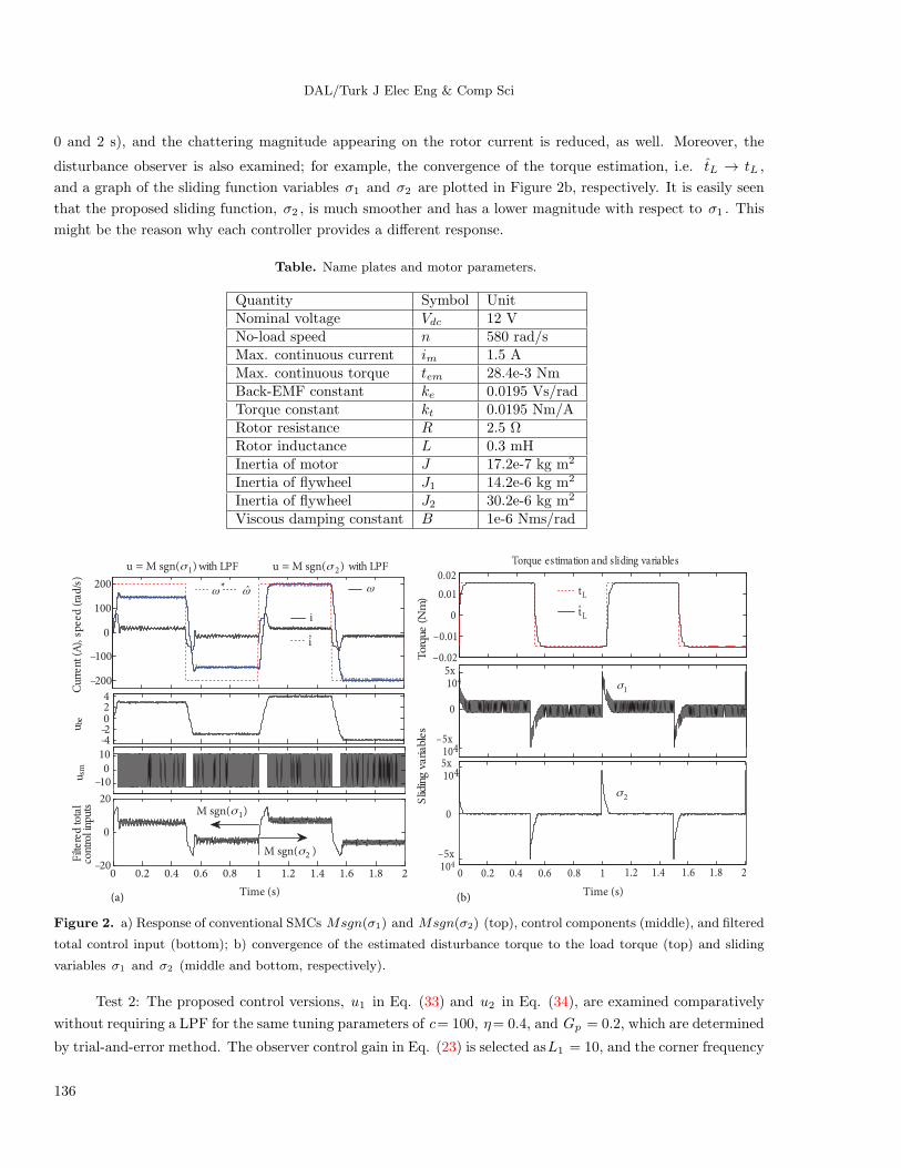
Test 1: In order to explore the properties of sliding functions σ1 and σ2 , these functions are examined
first by a conventional SMC, u = Msgn(σ) with a smoothing filter and a high magnitude gain M (=12). The
corner frequency of the LPF used in the torque observer is determined as 80 rad/s by the trial-and-error method.
The obtained results are shown comparatively in Figure 2a, where the speed tracking performance fails, and a
high magnitude of chattering (oscillation) arises on the rotor current when σ1 is used (between 0 and 1 s). In
contrast, a significant improvement in the speed tracking performance is achieved when σ2 is used (between
135
DAL/Turk J Elec Eng & Comp Sci
0 and 2 s), and the chattering magnitude appearing on the rotor current is reduced, as well. Moreover, the
disturbance observer is also examined; for example, the convergence of the torque estimation, i.e. tL → tL ,
and a graph of the sliding function variables σ1 and σ2 are plotted in Figure 2b, respectively. It is easily seen
that the proposed sliding function, σ2 , is much smoother and has a lower magnitude with respect to σ1 . This
might be the reason why each controller provides a different response.
Table. Name plates and motor parameters.
Quantity Symbol UnitNominal voltage Vdc 12 VNo-load speed n 580 rad/sMax. continuous current im 1.5 AMax. continuous torque tem 28.4e-3 NmBack-EMF constant ke 0.0195 Vs/radTorque constant kt 0.0195 Nm/ARotor resistance R 2.5 ΩRotor inductance L 0.3 mHInertia of motor J 17.2e-7 kg m2
Inertia of flywheel J1 14.2e-6 kg m2
Inertia of flywheel J2 30.2e-6 kg m2
Viscous damping constant B 1e-6 Nms/rad
–200
–100
0
100
200
Cur
rent
(A
), s
peed
(ra
d /s)
0 0.2 0.4 0.6 0.8 1 1.2 1.4 1.6 1.8 2–20
0
20
Filt
ered
t ota
lco
ntro
l inp
uts
–4–2024
–100
10
u sm
i
i
ω*ω ω
u be
with LPF)sgn( 1σMu = with LPF)sgn( 2σMu =
)sgn( 1σM
)sgn( 2σM
0
Slid
ing v
ariable
s
0 0.2 0.4 0.6 0.8 1 1.2 1.4 1.6 1.8 2
0
5x 10⁴
–0.02
–0.01
0
0.01
0.02
Torq
ue (
Nm
)
–5x10⁴
σ1
–5x 10⁴
5x 10⁴
σ 2
Lt
Lt
Torque estimation and sliding variables
(a) (b)Time (s) Time (s)
Figure 2. a) Response of conventional SMCs Msgn(σ1) and Msgn(σ2) (top), control components (middle), and filtered
total control input (bottom); b) convergence of the estimated disturbance torque to the load torque (top) and sliding
variables σ1 and σ2 (middle and bottom, respectively).
Test 2: The proposed control versions, u1 in Eq. (33) and u2 in Eq. (34), are examined comparatively
without requiring a LPF for the same tuning parameters of c= 100, η= 0.4, and Gp = 0.2, which are determined
by trial-and-error method. The observer control gain in Eq. (23) is selected asL1 = 10, and the corner frequency
136

DAL/Turk J Elec Eng & Comp Sci
of the LPF used in this observer is chosen as 75 rad/s. A comparative result is plotted in Figure 3a, where u1
is activated for the first half of the simulation time (between 0 and 1 s) and control version u2 takes place in
the second half of the simulation time (between 1 and 2 s). The components of each control version are plotted
separately in Figure 3b. These components, respectively, are the back-EMF denoted by ube ; the estimated
disturbance d(t); the discontinuous controls λsgn(σ1) and λsgn(σ2), both of which are denoted by usm ; and
the proportional error feedback denoted by ufb , whose significance arises at the transients.
–200
–150
–100
–50
0
50
100
150
200
0 0.2 0.4 0.6 0.8 1 1.2 1.4 1.6 1.8 2–20
–10
0
10
20
ˆ*ω ω ω
i
i
u2
u1
Cur
rent
(A
) an
d sp
eed
(rad
/s)
Con
trol
inp u
ts
u1 no filter u2 no filter
–5
0
5
–4000
0
4000
Co
mp
on
en
ts o
f co
ntr
ol u
1 a
nd
u2
–0.5
0
0.5
0 0.2 0.4 0.6 0.8 1 1.2 1.4 1.6 1.8 2
–100
–50
0
50
100
beu
smu
d
"u
(a) (b)Time (s) Time (s)
Figure 3. Response of the control versions: a) u1 and u2 (top), control inputs u1 and u2 (bottom); b) components of
control u1 (between 0 and 1 s) and u2 (between 1 and 2 s).
In the next simulation, Test 2 is repeated in order to explore how the performances of both control
versions, u1 and u2 , are affected when the disturbance d(t) is not injected. The obtained results are plotted
in Figure 4, where an unsatisfactory performance is obtained in the tracking and estimation of the speed
with respect to the previous test result shown in Figure 3, where injecting d(t) into each controller improves
the trajectory tracking performance. Moreover, without injecting d(t), the response of control u1 is adversely
affected more than that of control u2 . This can be observed clearly in Figure 4.
The next simulation is performed for a performance comparison between the proposed control version
u2 and the improved cascade PI current/speed control proposed in [21]. The relevant results are plotted in
Figure 5, where tracking of the rotor speed and current (top) and control signals uPI and u2 (bottom) are
shown in the left column and the magnified responses are shown in the right column. The superiority of the
proposed controller u2 with respect to the improved uPI controller arises with a faster response time, a better
suppression in current ripple, and no overshoot, which can be observed in the right column in Figure 5. These
comparative results also verify the fact that with proper selection of the sliding function, the performance of
the SMC can be improved.
In addition, several simulations are performed in order to explore the distinction between the controllers’
robustness and the variation of the speed. Therefore, all 3 control versions mentioned above are examined for
various speed ranges. First, the speed tracking performances of the controllers are examined under a constant
137

DAL/Turk J Elec Eng & Comp Sci
load (0.02 Nm) operation mode for a low range of reversal speed with 30 rad/s, and the obtained results are
plotted in Figure 6. Comparing the results in Figures 6a and 6b verifies that both proposed control versions,
u1 and u2 , provide lower speed ripple and lower current ripple with respect to improved uPI control. However,
at this low range of speed, the improved uPI control exhibits a faster transient response.
–200
–150
–100
–50
0
50
100
150
200
0 0.5 1 1.5 2–20
–10
0
10
20
Time (s)
u 1
ω*ω ω
u 2
i
i
Cu
rre
nt
(A)
an
d s
pe
ed
(ra
d/s
)C
on
tro
l in
pu
tsu1 no filter u2 no filter
Figure 4. The response of control versions u1 and u2 without the injection of the d(t) (top), control inputs (bottom).
-200
-150
-100
-50
0
50
100
150
200
Cu
rre
nt
(A)
an
d s
pe
ed
(ra
d/s
)
0 0.5 1 1.5 2-20
-10
0
10
20
Time (s)
Co
ntr
ol i
np
uts
0.5 0.6
-200
-150
-100
-50
0
50
100
150
200
1.5 1.6
-200
-100
0
100
200
ω*ω ω
i
i
i
i
Improved uPI and u2 Improved uPI
u2
ω
*ω
ω
u2
uPI
i
i
ω
*ω
ω
Figure 5. Reponses of the control u2 and improved uPI : tracking of the rotor speed and current (top) and control
inputs (bottom) in the left column, and magnified responses of uPI and u2 in the right column.
138

DAL/Turk J Elec Eng & Comp Sci
Cu
rre
nt
(A)
Sp
ee
d (
rad
/s)
uPI
–40
–30
–20
–10
0
10
20
30
40
0 0.2 0.4 0.6 0.8 1–40
–20
0
20
40
i i
ω
*ω
ω
i i
–40
–30
–20
–10
0
10
20
30
40
0 0.2 0.4 0.6 0.8 1 1.2 1.4 1.6 1.8 2–40
–20
0
20
40
u2
u1 no filte r u2 no filte r
Cu
rre
nt
(A)
Sp
ee
d (
rad
/s) u1
ω
*ω
ω
(a) (b)Time (s) Time (s)
Figure 6. Reponses of the controllers for a lower range reversal speed with 30 rad/s: a) for improved uPI , b) for both
u1 and u2 .
Moreover, the speed tracking performance is also examined under a constant load (0.02 Nm) operation
mode with varying stepped speed ranges (starting at 0 and increasing step-by-step to 50 rad/s, 100 rad/s, and
300 rad/s). The relevant results with an enlargement of the transients’ responses are plotted in Figure 7. As
mentioned above, in a sensorless drive, the improved uPI control version provides larger ripples and larger
overshoot in the current and speed with respect to the proposed control versions u1 and u2 . This can be seen
from comparing Figures 7a, 7b, and 7c, where the transient speed response time seems to be the same for all of
the control versions. For the later simulations, the current traces, i.e. i and i in Figures 6 and 7, are magnified
at a multiplication of 10 for better observation.
6. Hardware setup and experiments
6.1. Hardware setup
The experimental setup, called the DSP-2 DC experimental system, is shown in Figure 8. It consists of several
hardware and software components [16]. These are a small-sized PM DC (ESCAP) motor (with a low-resolution
encoder), a transistorized H-bridge power converter with a current and a voltage sensor, and a digital control
board called DSP-2. The DSP-2 controller, based on the TI TMS320C32-60 core and FPGA Xilinx CS40-
PQ240, can communicate with host PCs via a USB port with a serial RS-232 converter and has its own RCP
tools based on MATLAB/Simulink and the Real-Time Workshop toolbox. Thus, the control algorithms can be
easily programmed using the Simulink building blocks, and after the build-in process, the generated codes are
executed in real time within the DSP-2 controller. In all of the experiments, a sampling period of 200 µs is
used to execute the control algorithm. The software ‘Terminal’ running on the host PC provides a graphical
user interface for data visualization and parameter tuning while the system operates.
139

DAL/Turk J Elec Eng & Comp Sci
1
2
1
2
ω
*ω
ω
Cu
rre
nt
( A)
an
d S
pe
ed
(ra
d/s
)
uPI
0 0.5 1 1.5 2 2.5 3
0
50
100
150
200
250
300
350
0.9 1 1.1–20
0
20
40
60
80
100
120
ix10
10ˆxi
1.9 2 2.10
50
100
150
200
250
300
350
1
2
0 0.5 1 1.5 2 2.5 3–50
0
50
100
150
200
250
300
350
0.9 1 1.1–20
0
20
40
60
80
100
120
1.9 2 2.10
50
100
150
200
250
300
350
1
2
u2
Cu
rre
nt
(A)
an
d S
pe
ed
(ra
d/s
) ωω
*ω
ix10
10ˆxi
(a) (b)
1
2
0 0.5 1 1.5 2 2.5 3–50
0
50
100
150
200
250
300
350u3
0.9 1 1.1–20
0
20
40
60
80
100
120
1.9 2 2.10
50
100
150
200
250
300
350
ω
*ω
ω
ix10
10ˆxi
1
2
Cur
rent
(A
) an
d S
peed
(ra
d/s)
(c)
Time (s) Time (s)
Time (s)
Figure 7. Reponses of the controllers for stepped speed ranges for: a) the improved uPI , b) control version u1 , c) u2 .
Figure 8. DSP-2-based DC experimental system.
140

DAL/Turk J Elec Eng & Comp Sci
In order to load the motor, 2 differently sized aluminum flywheels, a small one with inertia J1 and a
large one with J2 , are used. The load variation is performed by exchanging these apparatuses consecutively,
i.e. each flywheel is mounted on the rotor shaft manually when the relevant study is required.
The overall configuration of the proposed control scheme is illustrated in Figure 9, where all of the
requisite control algorithms in the relevant blocks are programmed using MATLAB/Simulink, and executed by
the DSP-2 controller after the build-in process. In the control scheme, several software switches are employed in
order to perform an easy transition without repeating the build-in process, e.g., sw1 enables altering the speed
feedback signal between the estimated or measured one. Similarly, sw2 can alter control versions to activate
consecutively. Hence, sensored and sensorless drives using the proposed control versions can be used optionally,
making 1 or 0 the value on the pane of the parameter dialogue box shown on the DSP-2 terminal screen in
Figure 8.
H-Bridge
converter
Combined SMCs
(speed controller)
Eq . (33),(34)
Inc.Enc.
DC Link
Flywheel
(J1, J2)
Unified SM
current and
speed
observer (23)
M
i
u PWM
Modulator
VDC
Disturbance
observer (27)
Sliding
functions
Eq .(31),(32)
LTω i
ωω
*ω
Improved PI
cascaded controller
sw2
sw1
DSP-2 controller
Figure 9. Overall configuration of the proposed control scheme.
6.2. Experimental results
The performance of the sensored and sensorless SMC having a high magnitude gain was compared with the
conventional PI speed/current controller in [18]. Therefore, in this section, several comparative experiments
carried out on the DSP-2 experimental setup are presented in order to explore the distinction between the
proposed control laws and the others mentioned above. In all of the experiments, the design parameters, i.e. c
= 100, η = 0.5, and Gp = 0.5, determined by trial-and-error method are used.
Experiment 1: The first comparison is considered between the hybrid control version proposed in [18]
and the modified SMC version u1 . The second comparison is considered between the improved PI controller
proposed in [21] and the novel proposed control u2 . These tests are carried out while a light load (flywheel with
J1) acts on the rotor shaft and a reversal square-wave reference speed ω∗ = 200 rad/s is used. The response of
the high gain version SMC in [18] and u1 is plotted in Figure 10a; similarly, the response of the improved uPI
and u2 is plotted in Figure 10b. In this test, u1 and u2 are examined without injecting estimated disturbance
d(t). In this case, the obtained results verify that all of the control versions, u1 , u2 , and uPI , exhibit almost
the same performance in terms of speed tracking accuracy while the light load acts on the rotor shaft. However,
as can be seen in Figure 10a, proposed control laws u1 and u2 significantly reduce the magnitude of the current
ripple (or chattering) in respect to the significantly reduced chattering that arises on the rotor current in respect
141

DAL/Turk J Elec Eng & Comp Sci
to the control law proposed in [18], where a high gain (M = 12) and proportional error feedback were used.
It should be noted that in cascaded PI-based control schemes, the response time of the speed controller is
determined by the reference current, which is normally limited to 1.5 times the nominal load current of the
relevant motor. This is normally achieved by a limiter that is placed at the output of the speed controller.
However, the combined SMC scheme has a single-loop control structure and the unlikely cascaded structure of
the PI-based speed/current control scheme. Therefore, there is no mechanism that can limit the rotor current
reference; thus, inherently, it can reach a value of twice its nominal value depending on the acceleration of
the rotor shaft. Based on this, in the improved PI-controlled drive scheme, the reference current is limited
intentionally by twice its nominal value to make sure that the operation constraints are the same for all of the
compared control versions.
0.2 0.4 0.6 0.8
–200
–150
–100
–50
0
50
100
150
200
Cu
rre
nt
(A)
an
d s
pe
ed
(r a
d/s
)
and LPF
0.2 0.4 0.6
–200
–150
–100
–50
0
50
100
150
200
u1)sgn( 1σMu =
ω*ω ω ω*ω ω
i
i
i
i
0 0.2 0.4 0.6
–200
–150
–100
–50
0
50
100
150
200
u2
0 0.2 0.4 0.6–250
–200
–150
–100
–50
0
50
100
150
200
250
Cu
rre
nt
(A),
spe
ed
(ra
d/s
)
Improved uPI
ˆ
ii
ω*ω ωω*ω ω
ii
(a) (b)Time (s) Time (s)
Figure 10. Responses of the control versions for load inertia J1 : a) response of the SMC with the LPF and a high-
magnitude gain, and of control u1 ; b) response of u2 and the improved uPI .
Experiment 2: In order to explore the robustness of the proposed control laws with respect to the load
variation, experiment 1 is repeated for the flywheel with inertia J2 , which has a larger value with respect to
J1 . In this case, the obtained results regarding the rotor electromagnetic torque te (= ktxi) and estimated
load torque tL are shown in Figure 11a, where the graphics reflect the typical characteristics of the flywheel
acting on the rotor shaft. The variation of sliding variables σ1 and σ2 with respect to time are also plotted
in Figure 11b, which verifies that σ2 has a smoother and lower magnitude waveform than that of σ1 , which is
also verified in the simulation.
Performance comparisons between the improved PI control uPI and the proposed control versions (u1
and u2) are also performed. The responses of the controllers to the current and speed trajectories are shown in
Figure 12, where each control input and associated components are given in the left column. Control versions
u1 and u2 , are examined without injecting the disturbance d(t), and the obtained result is plotted in Figures
12a and 12b, respectively. The response of the improved uPI control version is shown in Figure 12c. All 3
controllers, uPI , u1 , and u2 , provide almost the same performance in the tracking of the speed and the current.
Concerning these results, it can be noted that the feedback component ufb suppresses the speed tracking error
at the transient instant for control versions u1 and u2 , and component ube compensates for the back-EMF
effect depending on the angular speed variations for all of the control versions.
142

DAL/Turk J Elec Eng & Comp Sci
0 0.5 1 1.5
-0.06
-0.04
-0.02
0
0.02
0.04
0.06
0.5 1 1.5-4
-3
-2
-1
0
1
2
3
4x 10⁴
1σ
2σ
et
x10- 4
Lt
Torque e s tima tion Sliding va ria ble s
To
rqu
e (
Nm
)
(a) (b)Time (s) Time (s)
Figure 11. a) Calculated electromagnetic torque te and estimated load torque tL , b) sliding variables σ1 and σ2 .
0 0.5 1 1.5
–200
–150
–100
–50
0
50
100
150
200
0 0.5 1 1.5–20
0
20–5
0
5
Co
mp
on
en
ts o
f co
nt r
ol u
1
–100
0
100
0.2 0.4 0.6180
210!u
beu
1u
smu
ω*ω ω
i
i
u1 without disturbance )(ˆ td
0 0.5 1 1.5
–200
–150
–100
–50
0
50
100
150
200
0 0.5 1 1.5–20
0
20–5
0
5–200
0
200
0.2 0.4 0.6180
210
smu
!u
2u
ˆ*ω ω ω
Co
mp
on
en
ts o
f co
ntr
ol u
2
i
ibeu
u2 without disturbance )(ˆ td
(a) (b)
0 0.5 1 1.5
–10
0
10
0 0.5 1 1.5
–200
–150
–100
–50
0
50
100
150
200
0 0.5 1 1.5
–5
0
5
0.2 0.4 0.6
180
200
PIu
beuω*ω ω
i
i
Improved uPI
Co
mp
on
en
ts o
f c
on
t ro
l u
PI
(c) Time (s)
Time (s)Time (s)
Figure 12. Responses in the tracking of the speed and current without injecting d(t) in both control versions: a) for
u1 and b) for u2 , respectively; c) response of the improved uPI .
143

DAL/Turk J Elec Eng & Comp Sci
However, from simulation results, it is expected that the response of control version u2 will be improved
by injecting disturbance signal d(t). To verify this, control u2 is examined by adding disturbance d(t), and the
provided result is plotted in Figure 13a, where a better performance is obtained in the tracking of the current
and the speed. In order to provide a better observation, a magnified response of the improved version uPI and
the proposed control versions u1 and u2 is plotted in Figure 13b, where it can be clearly seen that injecting
d(t) into control u2 improves the speed tracking at the transients and stabilizes the speed response in steady
state, as well as improving the convergence of the speed estimation. Moreover, proposed control u2 provides a
slightly faster transient response in respect to other control versions u1 and uPI , which can be seen in Figure
13b.
The variation of the load inertia (by exchanging the flywheels) is reflected as external disturbances
and/or mechanical parameter uncertainties in the drive system. Thus, the above results explore the controllers’
robustness to uncertainties caused by load variations. Moreover, all 3 control versions are examined for various
speed ranges in order to explore the controllers’ robustness to a variation of the speed under load operation
using the flywheel with J1 . First, the experiment is performed for a low-range reversal speed with 30 rad/s,
and the obtained results are plotted in Figure 14. Comparing the results shown in Figures 14a–14c verifies that
both of the proposed control versions, u1 and u2 , exhibit better performance with respect to the improved uPI
in speed tracking. The current ripples are almost the same for all of the control versions. However, u2 receives
a higher current at the transient instants at this low range of speed and u2 exhibits a faster transient response
with respect to u1 and the improved uPI .
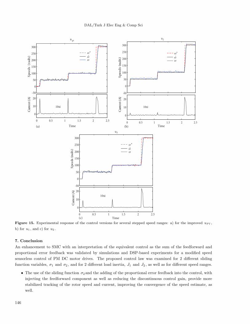
In addition, as done previously in Section 5, the speed tracking performance is also examined for varying
stepped speed ranges (starting at 0 and increasing step-by-step to 50 rad/s, 100 rad/s, and 300 rad/s) and
under a constant load (J1) operation. The relevant results are plotted in Figure 15. In the sensorless drive,
the improved uPI control version provides a larger overshoot in current and speed (see Figure 15a) with
respect to proposed control versions u1 and u2 (see Figures 15b and 15c), where u2 exhibits a better speed
tracking performance at 50 rad/s. In Figure 15, the currents are magnified at a multiplication of 10 for a better
observation.
–100
0
100
–5
0
5
Co
mp
on
en
t s o
f c
on
t ro
l u
2
0 0.5 1 1.5–20
0
20
0 0.5 1 1.5
–200
–150
–100
–50
0
50
100
150
200
0.2 0.4 0.6180
200
!u
ω*ω ω
2u
smubeud
u2 with dis turba nce )(ˆ td
i
i
Cu
rre
nt
(A),
s
pe
ed
(ra
d/s
)
0.1 0.2 0.3
u 2
0.1 0.2 0.3
u1
0.1 0.2 0.3
–200
–150
–100
–50
0
50
100
150
200
Improve d uPI
i
ω *ω
i
ω
(a) (b)Time (s) Time (s)
Figure 13. Response of the proposed control u2 : a) when disturbance signal is injected and b) a magnified performance
comparison for control versions uPI , u1 , and u2 , respectively.
144

DAL/Turk J Elec Eng & Comp Sci
40
–30
–20
–10
0
10
20
30
40
upi
0 0.2 0.4 0.6 0.8 1 1.2
–20
–10
0
10
20
Cu
rre
nt
(A)
10xi
ω
*ω
ω
ω
*ω
ω
–40
–20
0
20
40
u 2
0 0.2 0.4 0.6 0 .8 1 1.2
–20
0
20
Cu
rre
nt
(A)
(a)
(b)
–40
–30
–20
–10
0
10
20
30
40
0 0 .2 0 .4 0 .6 0 .8 1 1 .2
–20
0
20
10xi
u 3
Cu
rre
nt
(A)
Sp
ee
ds
(ra
d/ s
)
(c)
ω
*ω
ω
Time (s)Time (s)
Time (s)
Sp
ee
ds
(ra
d/ s
)
Sp
ee
ds
(ra
d/ s
)
Figure 14. Experimental response of the control versions for a lower range reversal speed with 30 rad/s: a) for the
improved uPI , b) for u1 , and c) for u2 .
145
DAL/Turk J Elec Eng & Comp Sci
–50
0
50
100
150
200
250
300
Speed
s (r
ad/s
)
u pi
0 0.5 1 1.5 2 2.5
0
10
20
Curr
en
t (A
)
Cur r
en
t ( A
)
10xi
ˆ
*ω
ωω
–50
0
50
100
150
200
250
300
Speed
s (r
ad/s
)
0 0.5 1 1.5 2 2.5
0
10
20
10xi
u2
ω
*ω
ω
(a) (b) Time Time
Time(c)
–50
0
50
100
150
200
250
300
Speeds
(rad/s
)
u3
0 0.5 1 1.5 2 2.5
0
10
20
10xi
Cu
rre
nt
(A)
ω
*ω
ω
Figure 15. Experimental response of the control versions for several stepped speed ranges: a) for the improved uPI ,
b) for u1 , and c) for u2 .
7. Conclusion
An enhancement to SMC with an interpretation of the equivalent control as the sum of the feedforward and
proportional error feedback was validated by simulations and DSP-based experiments for a modified speed
sensorless control of PM DC motor drives. The proposed control law was examined for 2 different sliding
function variables, σ1 and σ2 , and for 2 different load inertia, J1 and J2 , as well as for different speed ranges.
• The use of the sliding function σ2 and the adding of the proportional error feedback into the control, with
injecting the feedforward component as well as reducing the discontinuous control gain, provide more
stabilized tracking of the rotor speed and current, improving the convergence of the speed estimate, as
well.
146

DAL/Turk J Elec Eng & Comp Sci
• Moreover, significant chattering suppression and current ripple reduction were achieved by proposed
controls u1 and u2 , without requiring a smoothing LPF. The reduction of the current ripple means the
reduction of the torque pulsation in the motor drive control, which is a significant demand in industrial
applications where a precise torque control is required and the load inertia varies from a very small value
to a very large value (for example, paper machine winders). Thus, the proposed control version may be
extended to large machine drives.
• Although the proposed SMC scheme uses a single-loop control structure and does not require any addi-
tional chattering reduction techniques or a LPF, it is very easy to regulate the rotor speed and current in
a single loop, and the control performance is improved to some extent over that of the improved cascaded
PI current/speed control scheme. However, in the combined single-loop controller, there is no mechanism
to limit the rotor current, so it should be ensured that the rotor current is kept below the permitted
maximum current rating during operation.
The unified sliding mode observer performance was also examined with respect to the variation of the load
inertia, where the weakness of the observer occurs; thus, it necessitates that observer control gain L1 be
adapted to the load variation. Moreover, the convergence of the speed estimates fails at low speeds below 10
rad/s. This leads to the need for further study of the proposed control scheme improvement.
References
[1] Seborg DE, Edgar TF, Mellichamp DA. Process dynamics and control. New York, NY, USA: Wiley, 1989.
[2] Utkin VI. Variable structure systems with sliding modes. IEEE T Auto Contr 1977; 22: 212–222.
[3] DeCarlo RA, Zak SH, Matthews GP. Variable structure control of nonlinear multivariable systems: a tutorial. P
IEEE 1988; 76: 212–232.
[4] Hung JY, Gao WB, Hung JC. Variable structure control: a survey. IEEE T Ind Electron 1993; 40: 1–22.
[5] Utkin VI. Sliding mode control design principles and applications to electric drives. IEEE T Ind Electron 1993; 40:
23–35.
[6] Sabanovic A, Jezernik K, Sabanovic N. Sliding modes applications in power electronics and electrical drives. In:
Yu X, Xu JX, editors. Variable Structure Systems Towards the 21st Century. Berlin, Germany: Springer, 2002. pp.
223–251.
[7] Tan SC, Lai YM, Tse CK. General design issues of sliding-mode controllers in DC-DC converters. IEEE T Ind
Electron 2008; 55: 1160–1173.
[8] Edwards C, Spurgeon SK. Sliding Mode Control: Theory and Applications. London, UK: Taylor & Francis, 1998.
[9] Halil HK. Nonlinear Systems. New Jersey, NJ, USA: Pearson, 2000.
[10] Utkin VI, Gulder J, Shi J. Sliding Mode Control in Electromechanical Systems. London, UK: Taylor & Francis,
1999.
[11] Lee H, Utkin VI. Chattering suppression methods in sliding mode control systems. Annu Rev Control 2007; 31:
179–188.
[12] Fridman L. An averaging approach to chattering. IEEE T Automat Contr 2001; 46: 1260–1265.
[13] Xu JX, Pan YJ, Lee TH. Sliding mode control with closed-loop filtering architecture for a class of nonlinear systems.
IEEE T Circuits Syst 2004; 51: 168–173.
[14] Yu X, Kaynak O. Sliding-mode control with soft computing: a survey. IEEE T Ind Electron 2009; 56: 3275–3285.
147
DAL/Turk J Elec Eng & Comp Sci
[15] Ohnishi K, Matsui N, Hori Y. Estimation, identification, and sensorless control in motion control system. In: Bose
BK, editor. Power Electronics and Variable Frequency Drives: Technology and Applications. Piscataway, NJ, USA:
Wiley-IEEE Press, 1994. pp. 1253–1265.
[16] Hercog D, Curkovic M, Edilbehar G, Urlep E. Programming of the DSP-2 board with the MATLAB/Simulink. In:
IEEE 2003 International Conference on Industrial Technology; 10–12 December 2003. Maribor, Slovenia: IEEE. pp.
709–713.
[17] Slotine JJE, Li W. Applied Nonlinear Control. Englewood Cliffs, NJ, USA: Prentice-Hall, 1991.
[18] Dal M. DSP based sensorless PM DC motor drives using a proportional plus sliding mode control. In: IFAC 2009
2nd Intelligent Conference of Control Systems and Signal Processing; 21–23 September 2009. Istanbul, Turkey:
IFAC. pp. 1475–1479.
[19] Ohishi K, Nakao M, Ohnishi K. Microprocessor-controlled DC motor for load-insensitive position servo systems.
IEEE T Ind Electron 1987; 34: 44–49.
[20] Chang FJ, Twu SH, Chang S. Tracking control of DC motors via an improved chattering alleviation control. IEEE
T Ind Electron 1992; 39: 25–29.
[21] Buja GS, Menis R, Valla MI. Disturbance torque estimation in a sensorless DC Drive. IEEE T Ind Electron 1995;
42: 351–357.
[22] Pisano A, Davila A, Fridman L, Usai E. Cascade control of PM DC drives via second- order sliding-mode technique.
IEEE T Ind Electron 2008; 55: 3846–3854.
[23] Dal M, Teodorescu R. Sliding mode controller gain adaptation and chattering reduction techniques for DSP based
PM DC motor drives. Turk J Electr Eng Co 2011; 19: pp. 531–549.
148