CHAPTER 12

SIMULATED ANNEALING

12.1 ANNEALING AND PROBABILITY

Simulated annealing (SA) is a random search technique for global optimization problems, and it mimics the annealing process in material processing when a metal cools and freezes into a crystalline state with the minimum energy and larger crystal size so as to reduce the defects in metallic structures. The annealing process involves the careful control of temperature and cooling rate, often called annealing schedule.

The application of simulated annealing into optimization problems was pio­neered by Kirkpatrick, Gelatt and Vecchi in 1983. Since then, there have been extensive studies. Unlike the gradient-based methods and other determinis­tic search methods which have the disadvantage of being trapped into local minima, the main advantage of the simulated annealing is its ability to avoid being trapped in local minima. In fact, it has been proved that the simulated annealing will converge to its global optimality if enough randomness is used in combination with very slow cooling. In fact, simulated annealing algorithm is a search method using a Markov chain which converges under appropriate conditions concerning its transition probability.

Engineering Optimization: An Introduction with Metaheuristic Applications. 181 By Xin-She Yang Copyright © 2010 John Wiley & Sons, Inc.

182 CHAPTER 12. SIMULATED ANNEALING

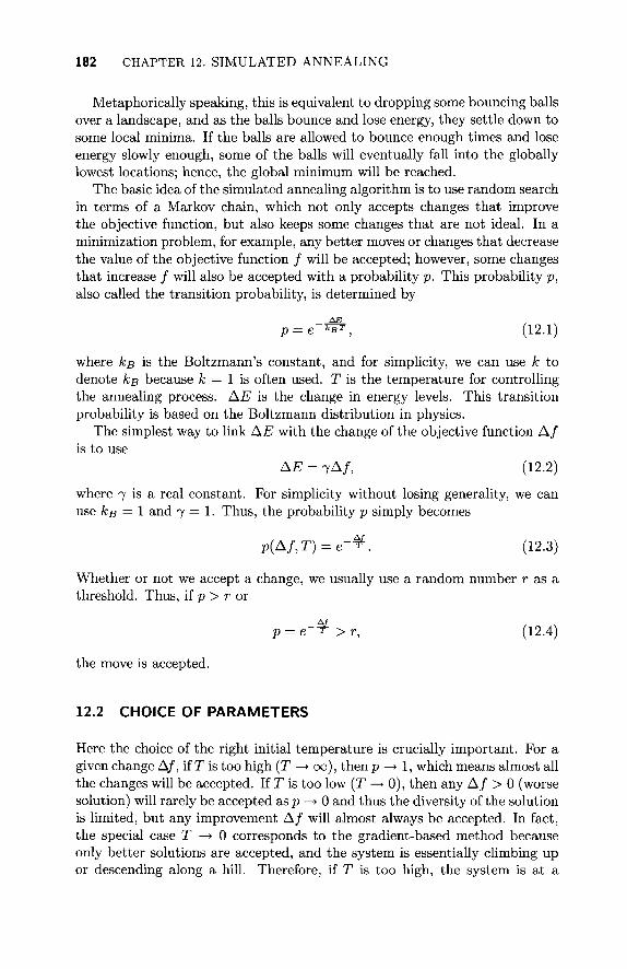
Metaphorically speaking, this is equivalent to dropping some bouncing balls over a landscape, and as the balls bounce and lose energy, they settle down to some local minima. If the balls are allowed to bounce enough times and lose energy slowly enough, some of the balls will eventually fall into the globally lowest locations; hence, the global minimum will be reached.

The basic idea of the simulated annealing algorithm is to use random search in terms of a Markov chain, which not only accepts changes that improve the objective function, but also keeps some changes that are not ideal. In a minimization problem, for example, any better moves or changes that decrease the value of the objective function / will be accepted; however, some changes that increase / will also be accepted with a probability p. This probability p, also called the transition probability, is determined by

ΔΕ p = e k B T , (12.1)

where kß is the Boltzmann's constant, and for simplicity, we can use k to denote kß because k — 1 is often used. T is the temperature for controlling the annealing process. AE is the change in energy levels. This transition probability is based on the Boltzmann distribution in physics.

The simplest way to link AE with the change of the objective function Δ / is to use

AE = 7 Δ / , (12.2)

where 7 is a real constant. For simplicity without losing generality, we can use fcß = 1 and 7 = 1 . Thus, the probability p simply becomes

p(Af,T) = e-¥. (12.3)

Whether or not we accept a change, we usually use a random number r as a threshold. Thus, if p > r or

Δ/ p = e T > r, (12-4)

the move is accepted.

12.2 CHOICE OF PARAMETERS

Here the choice of the right initial temperature is crucially important. For a given change Δ/ , if T is too high (T —> 00), then p —> 1, which means almost all the changes will be accepted. If T is too low (T —> 0), then any Δ / > 0 (worse solution) will rarely be accepted as p —> 0 and thus the diversity of the solution is limited, but any improvement Δ / will almost always be accepted. In fact, the special case T —> 0 corresponds to the gradient-based method because only better solutions are accepted, and the system is essentially climbing up or descending along a hill. Therefore, if T is too high, the system is at a

12.2 CHOICE OF PARAMETERS 183

Simulated Annealing Algorithm

Objective function f(x), x — (xi,...,xp)T

Initialize initial temperature To and initial guess x^ Set final temperature Tf and max number of iterations N Define cooling schedule T <—> aT, (0 < a < 1) while ( T > Tf and n< N )

Move randomly to new locations: xn+i — a;„+randn Calculate Δ / = / n + i ( x n + i ) - fn(xn) Accept the new solution if better i f not improved

Generate a random number r Accept if p = ε χ ρ [ - Δ / / Γ ] > r

end if Update the best x* and / * n — n+ 1

end while

Figure 12.1: Simulated annealing algorithm.

high energy state on the topological landscape, and the minima are not easily reached. If T is too low, the system may be trapped in a local minimum, not necessarily the global minimum, and there is not enough energy for the system to jump out the local minimum to explore other minima including the global minimum. So a proper initial temperature should be calculated.

Another important issue is how to control the annealing or cooling process so that the system cools down gradually from a higher temperature to ulti­mately freeze to a global minimum state. There are many ways of controlling the cooling rate or the decrease of the temperature.

Two commonly used annealing schedules (or cooling schedules) are: linear and geometric. For a linear cooling schedule, we have

T = To - ßt, (12.5)

or T —» T — 6T, where To is the initial temperature, and t is the pseudo time for iterations, β is the cooling rate, and it should be chosen in such a way that T —> 0 when t —> tf (or the maximum number ./V of iterations), this usually gives β = (To -Tf)/tf.

On the other hand, a geometric cooling schedule essentially decreases the temperature by a cooling factor 0 < a < 1 so that T is replaced by aT or

T(t) = TQa\ t = 1,2,...,«/. (12.6)

The advantage of the second method is that T —> 0 when t —> oo, and thus there is no need to specify the maximum number of iterations. For this reason,

184 CHAPTER 12. SIMULATED ANNEALING

we will use this geometric cooling schedule. The cooling process should be slow enough to allow the system to stabilize easily. In practise, a = 0.7 ~ 0.95 is commonly used.

In addition, for a given temperature, multiple evaluations of the objective function are needed. If too few evaluations, there is a danger that the system will not stabilize and subsequently will not converge to its global optimality. If too many evaluations, it is time-consuming, and the system will usually converge too slowly as the number of iterations to achieve stability might be exponential to the problem size.

Therefore, there is a fine balance between the number of evaluations and solution quality. We can either do many evaluations at a few temperature levels or do few evaluations at many temperature levels. There are two major ways to set the number of iterations: fixed or varied. The first uses a fixed number of iterations at each temperature, while the second intends to increase the number of iterations at lower temperatures so that the local minima can be fully explored.

12.3 SA ALGORITHM

The simulated annealing algorithm can be summarized as the pseudo code shown in Figure 12.1. In order to find a suitable starting temperature To, we can use any available information about the objective function. If we know the maximum change max(A/) of the objective function, we can use this to estimate an initial temperature To for a given probability po · That is

max(A/) J-o ~ ; ·

lnpo If we do not know the possible maximum change of the objective function, we can use a heuristic approach. We can start evaluations from a very high temperature (so that almost all changes are accepted) and reduce the temper­ature quickly until about 50% or 60% of the worse moves are accepted, and then use this temperature as the new initial temperature To for proper and relatively slow cooling processing.

For the final temperature, it should be zero in theory so that no worse move can be accepted. However, if Tf —■> 0, more unnecessary evaluations are needed. In practice, we simply choose a very small value, say, Tf = 10 - 1 0 ~ 10~5, depending on the required quality of the solutions and time constraints.

12.4 IMPLEMENTATION

Based on the guidelines of choosing the important parameters such as the cooling rate, initial and final temperatures, and the balanced number of it­erations, we can implement the simulated annealing using both Matlab and

12.4 IMPLEMENTATION 185

Figure 12.2: Rosenbrock's function with the global minimum f, = 0 at (1, l ) .

Figure 12.3: 500 evaluations during the simulated annealing. The final global best is marked with 0 .

Octave. The implemented Matlab and Octave program is given in Appendix B. Some of the simulations of the related test functions are explained in detail in the examples.

EXAMPLE 12.1

For Rosenbrock's banana function

f (x, y) = (1 - x ) ~ + 100(y - x2)2,

we know that its global minimum f, = 0 occurs at (1,l) (see Figure 12.2). This is a standard test function and quite tough for most conven-

186 CHAPTER 12. SIMULATED ANNEALING

Figure 12.4: The egg crate function with a global minimum f, = 0 at (0,O).

tional algorithms. However, using the program given in Appendix B, we can find this global minimum easily and the 500 evaluations during the simulated annealing are shown in Figure 12.3.

This banana function is still relatively simple as it has a curved narrow valley. Other functions such as the egg crate function are strongly multimodal and highly nonlinear. It is straightforward to extend the above program to deal with highly nonlinear multimodal functions. Let us look another example.

EXAMPLE 12.2

The egg crate function

f (x, y) = x2 + Y2 + 25[sin2(x) + in^(^)],

has the global minimum f, = 0 at (0,O) in the domain (x, y) E [-5,5] x [-5,5]. The landscape of the egg crate function is shown in Figure 12.4, and the paths of the search during simulated annealing are shown in Figure 12.5. It would takes about 2500 evaluations to get an optimal solution accurate to the third decimal place.

EXERCISES

12.1 Modify the program in Appendix B so as to investigate the rate of convergence of simulated annealing for different cooling schedules such as

Figure 12.5: The paths of moves of simulated annealing during iterations.

12.2 For standard SA, the cooling schedule is a monotonically decreasing function. There is no reason why we should not use other forms of cooling. For example, we can use

T(t) = To cos2 (t) exp[-at], a > 0.

Modify the SA program discussed in this book to study the behavior of various functions as a cooling schedule.

12.3 Write a program to find the minimum of the following function for any

where -27r < zi 5 27r.

12.4 Modify the Matlab program again to solve the following equality- constrained optimization

subject to an equality constraint

12.5 Modify the program of simulated annealing so as to use multiple par- allel chains for simulated annealing.

188 CHAPTER 12. SIMULATED ANNEALING

REFERENCES

1. C. Blum and A. Roli, "Metaheuristics in combinatorial optimization: Overview and conceptural comparison", ACM Comput. Sum., 35, 268-308 (2003).

2. G. W. Flake, The Computational Beauty of Nature: Computer Explorations of Fractals, Chaos, Complex Systems, and Adaptation, Cambridge, Mass.: MIT Press, 1998.

3. L. J. Fogel, A. J. Owens, and M. J. Walsh, Artificial Intelligence Through Sim-ulated Evolution, John Wiley & Sons, 1966.

4. S. Kirkpatrick, C. D. Gelatt, and M. P. Vecchi, "Optimization by simulated annealing", Science, 220, No. 4598, 671-680 (1983).

5. M. Molga, C. Smutnicki, "Test functions for optimization needs", http://www.zsd.ict.pwr.wroc.pl/files/docs/functions.pdf

6. I. Pavlyukevich, "Levy flights, non-local search and simulated annealing", J. Computational Physics, 226, 1830-1844 (2007).

7. W. H. Press, S. A. Teukolsky, W. T. Vetterling, B. P. Flannery, Numerical Recipes in C++: The Art of Scientific Computing, Cambridge University Press, 2002.

8. E.-G. Talbi, Metaheuristics: From Design to Implementation, John Wiley & Sons, 2009.