Engineering a high-performance SNP detection pipeline

Vasudevan Rengasamy Kamesh MadduriDepartment of Computer Science and Engineering

The Pennsylvania State UniversityUniversity Park, PA, USA

Email: vxr162@psu.edu, madduri@cse.psu.edu

April 18, 2015

Abstract

We present Sprite, a bioinformatic data analysis pipeline for detecting single nu-cleotide polymorphisms (SNPs) in the human genome. A SNP detection pipeline fornext-generation sequencing data uses several software tools, including tools for readpreprocessing, read alignment, and SNP calling. We target end-to-end scalability andI/O efficiency in Sprite by merging tools in this pipeline and eliminating redundan-cies. A key component of our optimized pipeline is parsnip, a new parallel method andsoftware tool for SNP calling. Experimental results on synthetic and real data sets in-dicate that the quality of results achieved by parsnip is comparable to state-of-the-artSNP calling software.

1 Introduction

In this work, we consider the pervasive genetic variation detection workflow in biomedical in-formatics. The goal of this workflow is to automatically determine genetic variations presentin the genome of an individual (called the donor), by comparing the donor genome to areference genome. Among structural variations, the most well-studied are Single NucleotidePolymorphisms, or SNPs. SNPs are nucleotide differences at a single position. Detect-ing these SNPs using current state-of-the-art tools can take more than a day of sequentialcompute time. We explain why this is the case in the next section. Our goal is to designparallel algorithms and identify optimizations to accelerate end-to-end performance of a SNPdetection (or SNP calling) pipeline.

Data reduction by two or three orders of magnitude is a common feature in most genomicdata analysis pipelines. The raw data, or data originating from the DNA sequencers, isusually in plain text format, compressed using gzip, and can be up to several 100 GB insize. Depending on the biological problem of interest, this data is processed in conjunctionwith additional data sets (which can be up to 1 TB), using a combination of analysis tools.

1

The output produced by the SNP detection software is much smaller and usually less than1 GB. The entire workflow is implemented as a script that executes different programs, andis either run on a dedicated server or submitted to the job scheduler of a shared cluster.A modular approach to pipeline construction is a poor match to current workstations, andalso results in very little overall speedup on supercomputers. For instance, the SMaSHbenchmarking effort [34] documents the performance of several variant detection pipelineson representative genomic data sets and a large shared-memory server. Running times arereported to be in the order of tens of hours to multiple days with state-of-the-art software,achieving a very small fraction of peak system performance.

There is a lot of current research on new algorithms and optimizations for various stages ofthis pipeline (reviewed in the next section). Our contributions in this paper follow the sametheme. Additionally, given that our end-goal is to identify SNPs, we explore possible ways forreduce unnecessary I/O, and design parallelization strategies with input data from currentsequencing technologies in mind. The current state-of-the-art deployments of this pipelineuse sequential software for certain stages, which turn out to be significant bottlenecks. Wehave focused our effort on the primary time-consuming steps in this paper and have designednew parallel algorithms and software (prune, sampa, parsnip) for these steps. The end-to-end running time of our pipeline on 16 nodes of the NERSC Edison supercomputer is around34 minutes for a realistic input data set. We also show that the resulting SNP detectionquality is comparable to a pipeline constructed using state-of-the-art tools. The end-to-endtime of the traditional pipeline is 28 hours, and so we achieve a nearly 49.5× speedup.

2 SNP Pipeline Overview

The genome sequences of any two (human) individuals are highly similar. However, the smallpercentage of genetic variation is believed to have important biological and medical implica-tions. Identifying an individual’s single nucleotide genetic variants has become a standardfirst step in many biological and biomedical applications. In this section, we describe theworkflow to detect these variants and prior approaches to exploit parallelism.

The output of a DNA sequencer is a set of reads. A read is a short segment of the genomewhose sequence is known, but whose location in the genome is not known. As sequencingdata becomes ubiquitous, standard workflows for its analysis are becoming commonly used.The basic idea is to align the reads against the human reference genome and identify genomiclocations where aligned reads show a variation in the nucleotide.

When sequence data is initially generated, it is typically stored on disk in multiple gzippedFASTQ (FQ) files. FQ is a text file format that stores each read using four lines, includingthe nucleotide sequence and the quality score of each nucleotide. FQ files are immediatelycompressed as they come off the sequencer. A single sequencing experiment will generatemultiple fq.gz files, with each file containing its own set of reads. FQ files are then putthrough several preprocessing filters, including the removal of low quality reads and trimmingreads to remove low quality nucleotides at the end. These filters are run separately on eachcompressed FQ file and the results are then written back to disk in the same format. The

2

Paired-end read files

.fq.gz

Reads aligned to reference

.sam .bam

Structural variants

Aligner(bwa)

Preprocessing(samtools)

Variant caller(freebayes)

.fq.gz

.vcf

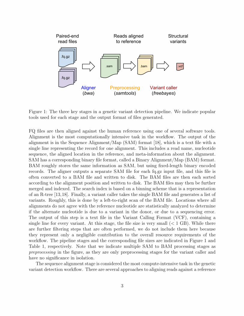
Figure 1: The three key stages in a genetic variant detection pipeline. We indicate populartools used for each stage and the output format of files generated.

FQ files are then aligned against the human reference using one of several software tools.Alignment is the most computationally intensive task in the workflow. The output of thealignment is in the Sequence Alignment/Map (SAM) format [18], which is a text file with asingle line representing the record for one alignment. This includes a read name, nucleotidesequence, the aligned location in the reference, and meta-information about the alignment.SAM has a corresponding binary file format, called a Binary Alignment/Map (BAM) format.BAM roughly stores the same information as SAM, but using fixed-length binary encodedrecords. The aligner outputs a separate SAM file for each fq.gz input file, and this file isoften converted to a BAM file and written to disk. The BAM files are then each sortedaccording to the alignment position and written to disk. The BAM files may then be furthermerged and indexed. The search index is based on a binning scheme that is a representationof an R-tree [13,18]. Finally, a variant caller takes the single BAM file and generates a list ofvariants. Roughly, this is done by a left-to-right scan of the BAM file. Locations where allalignments do not agree with the reference nucleotide are statistically analyzed to determineif the alternate nucleotide is due to a variant in the donor, or due to a sequencing error.The output of this step is a text file in the Variant Calling Format (VCF), containing asingle line for every variant. At this stage, the file size is very small (< 1 GB). While thereare further filtering steps that are often performed, we do not include them here becausethey represent only a negligible contribution to the overall resource requirements of theworkflow. The pipeline stages and the corresponding file sizes are indicated in Figure 1 andTable 1, respectively. Note that we indicate multiple SAM to BAM processing stages aspreprocessing in the figure, as they are only preprocessing stages for the variant caller andhave no significance in isolation.

The sequence alignment stage is considered the most compute-intensive task in the geneticvariant detection workflow. There are several approaches to aligning reads against a reference

3

Table 1: The output format and typical file sizes of various steps in a SNP calling pipeline.

Step Output Format Typical Size

Read preprocessing multiple fq.gz 240 GBAlignment multiple SAM 130 GBBinary encode, sort, merge multiple BAM 130 GBVariant calling single VCF < 1 GB

genome. Usually, an alignment algorithm uses an index of the reference genome. The FM-index [9] is the index of choice for the most popular aligners of sequencing data [15, 17, 20].It can be used to find if a query substring occurs in the reference in time independent of thelength of the reference. The FM-index is a full-text index which is based on the Burrows-Wheeler transform [1, 5] developed for text compression. The implementation of the FM-index stores the Huffman-coded Burrows-Wheeler transform of the reference string alongwith two associated arrays and some neglible space overhead. In addition to alignment, it isused in other bioinformatic areas such as de novo genome assembly [16,32,33] and sequencingdata analysis [31]. An alternate to the FM-index is hash-based index. In this approach, ahash table is created mapping all small strings (called seeds) to their locations in the reference(or, sometimes, in the reads). While initially popular [19, 30], hash-based approaches havelargely been replaced by the FM-index approach due to its superior performance.

There are two main tasks that an alignment software package performs: (1) constructingan index given the set of reference sequences (a one-time operation in most pipelines), and(2) aligning reads to the reference sequences by accessing the index. While there is somework on parallelizing FM-index construction and its underlying subroutines [8], most currentefforts on parallelizing alignment software focus on the alignment step, and prebuilt indexesare available for commonly-used reference sequences. In a shared-memory environment, theindex is loaded into memory and reads are partitioned across multiple threads. This is thepredominant parallelization strategy employed in most x86-based software, and the latestversions of BWA and Bowtie 2 already support multithreading. There is however a lot ofroom for improvement in these multithreaded implementations. Zhang et al. [37] profileperformance of BWA on an Intel Sandy Bridge-based system and observe that the dominantsubroutine is the backward search step. This step involves a tree traversal and results insignificant cache and TLB misses. Computational load imbalances due to coarse-grainedread partitioning can also lead to performance slowdown. Martınez et al. propose a dynamicread reordering scheme [25] for RNA sequence matching. There are also several recently-developed CUDA implementations for NVIDIA GPUs, such as SOAP3 [21], BarraCUDA [14],and CUSHAW [23]. NVIDIA has released the NVBIO software package [28], which providesCUDA subroutines that can be reused by bioinformatics tasks, and also includes a CUDAport of BWA. CUSHAW2-GPU [22] is a notable recent aligner that partitions reads acrossthe host and the GPU. There are also aligners using FPGAs [24, 35]. Convey computer,using their HC-Series hybrid core hardware and tuned bioinformatics software, report whatwe believe are the current-best speedup results (15–20×) over BWA on multicore servers [6].

4

There are also parallel hash-based aligners such as SNAP [36], which are significantly fasterthan BWA and Bowtie 2. However, execution time is only one of the many criteria usedto assess alignment software. Hatem et al. [12] compare several different x86 aligners usingcriteria such as mapping quality, support for gapped alignments, memory footprint, supportfor inexact matches, in addition to execution time. Their main conclusion is that there isno clear winner. Alignment is thus still an open problem and an active topic of currentresearch. Note however that the relative proportions of time spent in various pipeline tasksdepend on the hardware configuration, the software tools used for the tasks and the level ofoptimization they employ, and the specific problem solved using the pipeline. Amdahl’s lawwill drastically limit overall speedups for any efforts that focus exclusively on the alignmentstage.

Parallel I/O optimization, in the context of the genetic variant pipeline, has not re-ceived much attention. Recent work that is most relevant to the proposed research is SeqIn-Cloud [26], a Windows Azure implementation of a genomics pipeline that comprises BWAand GATK. This pipeline implementation uses CRAM [10], a lossless alignment output al-ternative to the BAM file format, and reduces storage costs on this Azure deployment. Twopopular approaches to support parallel sequence search are query partitioning and referencepartitioning. Query partitioning implies splitting up the reads among multiple tasks andreplicating the reference database. A more scalable strategy, used in tools such as mpi-BLAST [7], is reference partitioning. Here, each processor searches whole query sequencesagainst a fraction of the reference. Zhu et al. [38] investigate I/O behavior with mpiBLASTfor different I/O access schemes, and study the performance impact of the degree of I/Oparallelism and the contention of I/O resources on parallel BLAST. It is also one of thefirst papers to examine the impact of I/O contention on genomics pipelines. BLAST [2] is aclassical alignment tool, albeit it is not suitable for the type of data used in variant detectionworkflows. Because of its popularity in other applications, however, it has been a focus ofI/O optimization efforts.

3 The SPRITE Analysis Pipeline

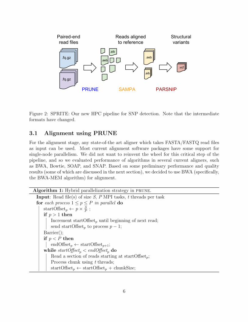
We now present our new SNP calling pipeline called Sprite and explain the rationale be-hind creating new modules. Sprite is made up of three tools, prune, sampa, and parsnip,roughly corresponding to the three key steps of alignment, preprocessing, and variant detec-tion, indicated in the previous section. Figure 2 shows the pipeline stages. Note that theintermediate file formats have changed in this case, but we still work with the restriction ofusing FQ as input and generating VCF-formatted output files. Our pipeline is designed toexploit both shared- and distributed-memory parallelism as much as possible. We use theMPI library for inter-process parallelism and POSIX threads in shared memory. We use theterms MPI task and MPI process interchangeably in discussion below.

5

Paired-end read files

.fq.gz

Reads aligned to reference

.aeb

Structural variants

PRUNE SAMPA PARSNIP

.fq.gz

.vcf

.aib

.aeb

.aib

Figure 2: SPRITE: Our new HPC pipeline for SNP detection. Note that the intermediateformats have changed.

3.1 Alignment using PRUNE

For the alignment stage, any state-of-the art aligner which takes FASTA/FASTQ read filesas input can be used. Most current alignment software packages have some support forsingle-node parallelism. We did not want to reinvent the wheel for this critical step of thepipeline, and so we evaluated performance of algorithms in several current aligners, suchas BWA, Bowtie, SOAP, and SNAP. Based on some preliminary performance and qualityresults (some of which are discussed in the next section), we decided to use BWA (specifically,the BWA-MEM algorithm) for alignment.

Algorithm 1: Hybrid parallelization strategy in prune.

Input: Read file(s) of size S, P MPI tasks, t threads per taskfor each process 1 ≤ p ≤ P in parallel do

startOffsetp ← p× SP

;if p > 1 then

Increment startOffsetp until beginning of next read;send startOffsetp to process p− 1;

Barrier();if p < P then

endOffsetp ← startOffsetp+1;while startOffsetp < endOffsetp do

Read a section of reads starting at startOffsetp;Process chunk using t threads;startOffsetp ← startOffsetp + chunkSize;

6

BWA only supports shared-memory parallelism via POSIX threads. One simple andcommonly-used approach to distributed-memory parallelization is read partitioning and ref-erence sequence replication. For instance, the MPI-based tool pMap [4] provides multi-nodeparallelism for different aligner software using reference replication. The tool divides workamong multiple tasks by assigning a portion of read files to each MPI task. Our overallparallelization strategy is similar to pMap. Instead of just calling the BWA binary as-is ona smaller read file (like what is done in pMap), we modify the latest source code of BWA.These changes were motivated by the following reasons:

• The output of BWA, like other aligners, is a SAM file. SAM is a tab-separated textfile briefly described in the previous section. Not all fields present in the SAM file arerequired for variant calling.

• The textual records should be parsed to obtain usable field values by downstream toolsin order to reorder and index the alignments.

Existing pipelines require that the SAM files(s) be converted to BAM file(s) to easeprocessing the alignment records. We shift some of the burden of downstream SAM fileprocessing to the alignment stage itself, and this has led to make the following modificationsto BWA.

• We exploit hybrid MPI and pthread parallelism to enable BWA to scale across multiplenodes.

• We generate separate alignment files for each contig (or contiguous sequences withoutgaps) in the reference sequence. The reference comprises several large contigs. Achromosome, for instance, could be a contig. In reality, there are about a hundredcontigs of different lengths in the reference.

• We generate alignment records for the cases of full and partial match cases of align-ments. We directly create binary output files of alignment records with condensedinformation.

We refer to our current implementation of this aligner with the above changes as prune.Some key implementation details of these modifications are discussed in the following sub-sections. Note that we can also generate full SAM files with prune, if necessary.

3.1.1 Hybrid MPI and POSIX thread parallelism

In BWA-MEM, the number of threads to be created can be specified using the command lineoption -t. BWA proceeds by reading a chunk of reads, which are processed by the threads inparallel, and a chunk of alignment records are written to the output SAM file. In our MPIparallelization, each task is assigned a fixed number of reads to align. A task in-turn chunksthese reads and assigns to individual threads to process them.

Algorithm 1 summarizes our hybrid parallelization scheme. The input read files canbe in compressed or uncompressed format, and hence BWA uses the zlib function gzread for

7

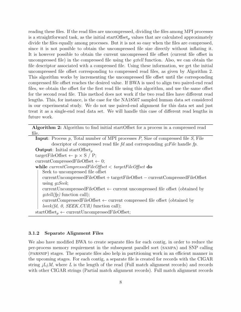
reading these files. If the read files are uncompressed, dividing the files among MPI processesis a straightforward task, as the initial startOffsetp values that are calculated approximatelydivide the files equally among processes. But it is not so easy when the files are compressed,since it is not possible to obtain the uncompressed file size directly without inflating it.It is however possible to obtain the current uncompressed file offset (current file offset inuncompressed file) in the compressed file using the gztell function. Also, we can obtain thefile descriptor associated with a compressed file. Using these information, we get the initialuncompressed file offset corresponding to compressed read files, as given by Algorithm 2.This algorithm works by incrementing the uncompressed file offset until the correspondingcompressed file offset reaches the desired value. If BWA is used to align two paired-end readfiles, we obtain the offset for the first read file using this algorithm, and use the same offsetfor the second read file. This method does not work if the two read files have different readlengths. This, for instance, is the case for the NA18507 sampled human data set consideredin our experimental study. We do not use paired-end alignment for this data set and justtreat it as a single-end read data set. We will handle this case of different read lengths infuture work.

Algorithm 2: Algorithm to find initial startOffset for a process in a compressed readfile.

Input: Process p, Total number of MPI processes P, Size of compressed file S, Filedescriptor of compressed read file fd and corresponding gzFile handle fp.

Output: Initial startOffsetptargetFileOffset ← p × S / P;currentCompressedFileOffset ← 0;while currentCompressedFileOffset < targetFileOffset do

Seek to uncompressed file offsetcurrentUncompressedFileOffset + targetFileOffset− currentCompressedFileOffsetusing gzSeek;currentUncompressedFileOffset ← current uncompressed file offset (obtained bygztell(fp) function call);currentCompressedFileOffset ← current compressed file offset (obtained bylseek(fd, 0, SEEK CUR) function call);

startOffsetp ← currentUncompressedFileOffset;

3.1.2 Separate Alignment Files

We also have modified BWA to create separate files for each contig, in order to reduce theper-process memory requirement in the subsequent parallel sort (sampa) and SNP calling(parsnip) stages. The separate files also help in partitioning work in an efficient manner inthe upcoming stages. For each contig, a separate file is created for records with the CIGARstring ¡L¿M, where L is the length of the read (Full match alignment records) and recordswith other CIGAR strings (Partial match alignment records). Full match alignment records

8

doesn’t have any insertions, deletions or soft/hard clipping, and as a result, are easier toprocess downstream.

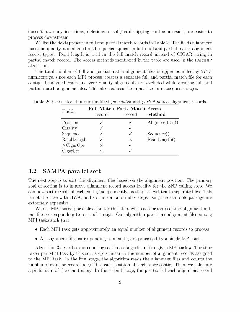
We list the fields present in full and partial match records in Table 2. The fields alignmentposition, quality, and aligned read sequence appear in both full and partial match alignmentrecord types. Read length is used in the full match record instead of CIGAR string inpartial match record. The access methods mentioned in the table are used in the parsnipalgorithm.

The total number of full and partial match alignment files is upper bounded by 2P ×num contigs, since each MPI process creates a separate full and partial match file for eachcontig. Unaligned reads and zero quality alignments are excluded while creating full andpartial match alignment files. This also reduces the input size for subsequent stages.

Table 2: Fields stored in our modified full match and partial match alignment records.

Full Match Part. Match AccessField

record record Method

Position X X AlignPosition()Quality X XSequence X X Sequence()ReadLength X × ReadLength()#CigarOps × XCigarStr × X

3.2 SAMPA parallel sort

The next step is to sort the alignment files based on the alignment position. The primarygoal of sorting is to improve alignment record access locality for the SNP calling step. Wecan now sort records of each contig independently, as they are written to separate files. Thisis not the case with BWA, and so the sort and index steps using the samtools package areextremely expensive.

We use MPI-based parallelization for this step, with each process sorting alignment out-put files corresponding to a set of contigs. Our algorithm partitions alignment files amongMPI tasks such that

• Each MPI task gets approximately an equal number of alignment records to process

• All alignment files corresponding to a contig are processed by a single MPI task.

Algorithm 3 describes our counting sort-based algorithm for a given MPI task p. The timetaken per MPI task by this sort step is linear in the number of alignment records assignedto the MPI task. In the first stage, the algorithm reads the alignment files and counts thenumber of reads or records aligned to each position of a reference contig. Then, we calculatea prefix sum of the count array. In the second stage, the position of each alignment record

9

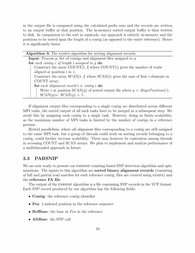
in the output file is computed using the calculated prefix sum and the records are writtento an output buffer at that position. The in-memory sorted output buffer is then writtento disk. In comparison to the sort in samtools, our approach is entirely in-memory and thepositions to be sorted span the length of a contig (as opposed to the entire reference). Henceit is significantly faster.

Algorithm 3: The sampa algorithm for sorting alignment records.

Input: Process p, Set of contigs and alignment files assigned to pfor each contig c of length l assigned to p do

Construct the array COUNT[1..l] where COUNT(i) gives the number of readsaligned at position i in c;Construct the array SCAN[1..l] where SCAN(i) gives the sum of first i elements inCOUNT array;for each alignment record r ∈ contig c do

Write r at position SCAN(p) of sorted output file where p = AlignPosition(r);SCAN(p)← SCAN(p) + 1;

If alignment output files corresponding to a single contig are distributed across differentMPI tasks, the sorted output of all such tasks have to be merged in a subsequent step. Weavoid this by assigning each contig to a single task. However, doing so limits scalability,as the maximum number of MPI tasks is limited by the number of contigs in a referencegenome.

Hybrid parallelism, where all alignment files corresponding to a contig are still assignedto the same MPI task, but a group of threads could work on sorting records belonging to acontig, could further increase scalability. There may however be contention among threadsin accessing COUNT and SCAN arrays. We plan to implement and analyze performance ofa multithreaded approach in future.

3.3 PARSNIP

We are now ready to present our parsnip counting-based SNP detection algorithm and opti-mizations. The inputs to this algorithm are sorted binary alignment records (consistingof full and partial read matches for each reference contig; files are created using sampa) andthe reference FA file.

The output of the parsnip algorithm is a file containing SNP records in the VCF format.Each SNP record produced by our algorithm has the following fields:

• Contig: the reference contig identifier

• Pos: 1-indexed position in the reference sequence

• RefBase: the base at Pos in the reference

• AltBase: the SNP call

10

3

1

A G G T A C T C C A T T C T A

1 L

Ref

G

T

C

A

AACA

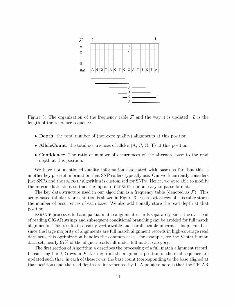
Figure 3: The organization of the frequency table F and the way it is updated. L is thelength of the reference sequence.

• Depth: the total number of (non-zero quality) alignments at this position

• AlleleCount: the total occurrences of alleles (A, C, G, T) at this position

• Confidence: The ratio of number of occurrences of the alternate base to the readdepth at this position.

We have not mentioned quality information associated with bases so far, but this isanother key piece of information that SNP callers typically use. Our work currently considersjust SNPs and the parsnip algorithm is customized for SNPs. Hence, we were able to modifythe intermediate steps so that the input to parsnip is in an easy-to-parse format.

The key data structure used in our algorithm is a frequency table (denoted as F). Thisarray-based tabular representation is shown in Figure 3. Each logical row of this table storesthe number of occurrences of each base. We also additionally store the read depth at thatposition.

parsnip processes full and partial match alignment records separately, since the overheadof reading CIGAR strings and subsequent conditional branching can be avoided for full matchalignments. This results in a easily vectorizable and parallelizable innermost loop. Further,since the large majority of alignments are full match alignment records in high-coverage readdata sets, this optimization handles the common case. For example, for the Venter humandata set, nearly 97% of the aligned reads fall under full match category.

The first section of Algorithm 4 describes the processing of a full match alignment record.If read length is l, l rows in F starting from the alignment position of the read sequence areupdated such that, in each of these rows, the base count (corresponding to the base aligned atthat position) and the read depth are incremented by 1. A point to note is that the CIGAR

11

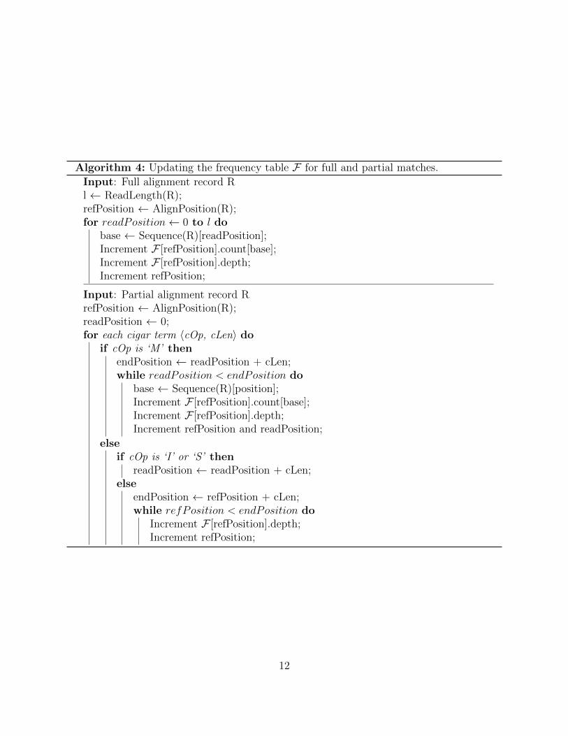
Algorithm 4: Updating the frequency table F for full and partial matches.

Input: Full alignment record Rl ← ReadLength(R);refPosition ← AlignPosition(R);for readPosition← 0 to l do

base ← Sequence(R)[readPosition];Increment F [refPosition].count[base];Increment F [refPosition].depth;Increment refPosition;

Input: Partial alignment record RrefPosition ← AlignPosition(R);readPosition ← 0;for each cigar term 〈cOp, cLen〉 do

if cOp is ‘M’ thenendPosition ← readPosition + cLen;while readPosition < endPosition do

base ← Sequence(R)[position];Increment F [refPosition].count[base];Increment F [refPosition].depth;Increment refPosition and readPosition;

elseif cOp is ‘I’ or ‘S’ then

readPosition ← readPosition + cLen;else

endPosition ← refPosition + cLen;while refPosition < endPosition do

Increment F [refPosition].depth;Increment refPosition;

12

operation M (Match) also contain SNPs, and all read bases in the matched positions neednot actually match with the corresponding bases in the reference sequence.

For partial alignment records, the CIGAR string output of BWA consists of the followingoperations as described in the SAM Format Specification document [18].

• M - Match. This is the only operation which could contribute to SNPs.

• I - Insertion, D - Deletion, S - Soft clipping, H - Hard clipping.

As shown in Algorithm 4, partial alignment records are processed by iterating throughthe CIGAR operations. Each operation in the CIGAR string is a tuple consisting of CIGARoperation type cOp and length cLen of the reference sequence/read on which this operationshould be applied.

If the operation is Match, the base count and depth fields of F are incremented for thematched positions, similar to the full match case described previously. If the operation isDeletion, then the depth field alone is incremented for these positions, since it indicates agap character in these positions. For other operations, cLen bases are skipped in the alignedread to process the next CIGAR operation.

3.3.1 Parallelization

We use MPI to parallelize parsnip. The sorted full and partial match alignment files aremapped to MPI tasks in a many-to-one manner. Our mapping also ensures that

1. Each MPI task gets approximately equal number of alignment records to process.

2. Both the full and partial alignment record files corresponding to a contig are assigned tothe same MPI task. This avoids the need to combine the partial entries in the frequencytable F from different MPI tasks. Such a scenario could occur if files corresponding tothe same contig are assigned to different MPI tasks.

After mapping input files to the MPI tasks, each task proceeds by reading a chunk ofrecords (100,000) at a time, and processing them as described in Algorithm 4, depending onthe record type read.

As is the case with the sampa step discussed in the previous section, parsnip is pleasantlyparallel, since each MPI task has its own set of input files and creates separate output filescontaining the SNP records of the contigs that were assigned to it.

3.3.2 Algorithm Complexity

Both full and partial match algorithms run in time that is linear in terms of the length ofthe aligned reads. F is the major memory-consuming data structure. With parsnip, eachMPI task requires only the current contig’s frequency table F to be in memory. For humanreference genome, the longest contig length is around 250 million base pairs corresponding tothe contig chr10. A row in the F corresponding to one position of reference contig requires 11

13

bytes. So the largest contig requires approximately 2.75 GB memory, which is the maximummemory required per process. As larger number of MPI tasks are created per node, memorycould become a potential bottleneck. This could be again be alleviated by hybrid parallelism,where 1 MPI task per process is created and multiple threads are created, and these threadswithin a task cooperate to process different alignment records corresponding to the samecontig. While this is a straightforward extension, we leave this for future work, as the runningtimes of both parsnip and sampa are extremely low compared to their counterparts in thereference pipeline.

4 Performance Results

In this section, we compare performance and quality results using tools in our new Spritepipeline to a reference pipeline with popular and commonly-used bioinformatics tools.

4.1 Experimental Setup

For all our experiments, we used the Edison supercomputer at the National Energy ResearchScientific Computing center (NERSC) in California, USA. Edison is a Cray XC30 systemwith a peak floating-point performance of 2.57 PF/s, with a total of 5,576 compute nodesand 133,824 cores. Each compute node has two 12-core Intel Ivy Bridge processors. Eachnode also has 64 GB DDR3 memory. We build all the programs using the Intel C compilerand the Cray Programming Environment. Our input files are stored on of the local scratchpartitions of Edison. We use a file stripe size of 8 MB and set large stripe settings to spreaddata across multiple I/O nodes.

We used the following four data sets, downloaded from the SMaSH website [29]. Threeof them use the human genome as reference, and one is based on the mouse genome.

• Venter: this is a synthetic human dataset created by inserting HuRef variants [3] intothe hg19 reference genome.

• NA12878 and NA18507: these are real human datasets consisting of high-coverageIllumina reads.

• Mouse: this is a real dataset consisting of paired-end reads from the B6 mouse strain.

The SMaSH benchmarking article [34] describes these data sets in more detail and explainstheir creation process. The website also gives running times and variant detection qualityinformation for several different combinations of tools in the pipeline we have been focusingon.

Table 3 mentions the list of software tools that we used to build the reference pipeline. Wehave evaluated Sprite’s accuracy and efficiency by comparing our results to ones obtainedfrom the reference pipeline. These tools were picked because of the combination of speedand result quality, as documented on the webpage.

14

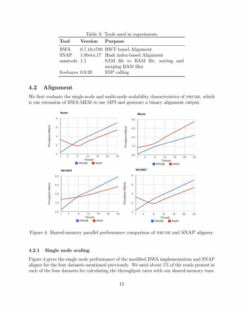
Table 3: Tools used in experiments

Tool Version Purpose

BWA 0.7.10-r789 BWT-based AlignmentSNAP 1.0beta.17 Hash index-based Alignmentsamtools 1.1 SAM file to BAM file, sorting and

merging BAM filesfreebayes 0.9.20 SNP calling

4.2 Alignment

We first evaluate the single-node and multi-node scalability characteristics of prune, whichis our extension of BWA-MEM to use MPI and generate a binary alignment output.

Venter

PRUNE SNAP

1 4 8 12 16 20 240

2

4

6

8

Threads

Thro

ughp

ut (M

bp/s

)

Mouse

PRUNE SNAP

1 4 8 12 16 20 240.0

1.5

3.0

4.5

6.0

Threads

Thro

ughp

ut (M

bp/s

)

NA12878

PRUNE SNAP

1 4 8 12 16 20 240.0

1.5

3.0

4.5

6.0

Threads

Thro

ughp

ut (M

bp/s

)

NA18507

PRUNE SNAP

1 4 8 12 16 20 240

2

4

6

8

Threads

Thro

ughp

ut (M

bp/s

)

Figure 4: Shared-memory parallel performance comparison of prune and SNAP aligners.

4.2.1 Single node scaling

Figure 4 gives the single node performance of the modified BWA implementation and SNAPaligner for the four datasets mentioned previously. We used about 1% of the reads present ineach of the four datasets for calculating the throughput rates with our shared-memory runs.

15

These correspond to around 9 million (Venter), 15.6 million (Mouse), 16 million (NA12878),and 14 million (NA18507) reads. We note that the performance of original BWA-MEM is verysimilar to prune, and hence we do not report its results. SNAP uses a different algorithmicstrategy for indexing and hence we chose to compare performance to our approach.

Due to the hash index-based seed lookup, SNAP’s single core performance is significantlybetter than that of BWA. But it can be seen that, BWA scales better than SNAP, especiallywhen the number of threads is increased from 1 to 8. This could be because in Edison, eachcompute node has 2 sockets with 12 cores each and these 12 cores have shared access to L3cache. SNAP assigns a range of reads to each core and hence when each core brings in a setof reads into L3 cache. It is likely that cores evict each other’s read chunks, and this maylead to more cache misses. In comparison, BWA reads a chunk of reads, and each threadworks towards mapping some of these reads. We believe this could be one possible reasonfor the performance gap. On 24 threads, SNAP is faster than prune only for the mousegenomic data. We will need to further investigate the reasons for this performance switch.Another aspect to mention is that these alignments were carried out using the paired-endsetting, which are often slower than single-ended alignment.

4.2.2 Multi-node scaling

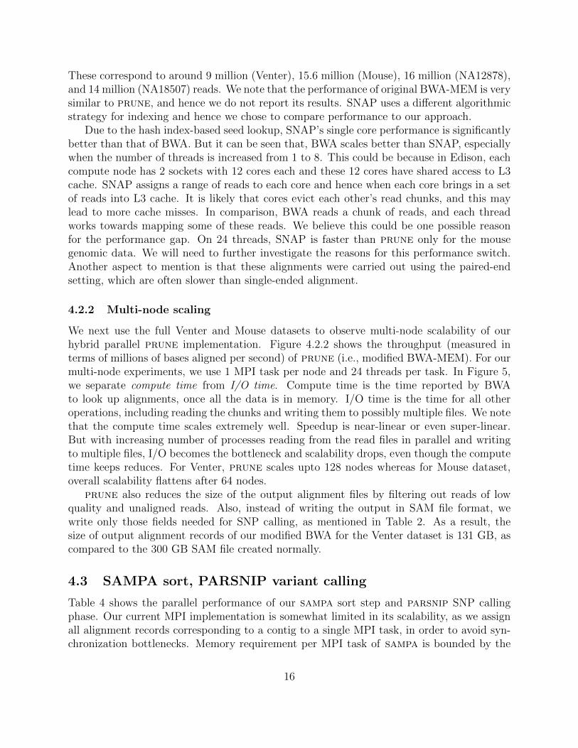
We next use the full Venter and Mouse datasets to observe multi-node scalability of ourhybrid parallel prune implementation. Figure 4.2.2 shows the throughput (measured interms of millions of bases aligned per second) of prune (i.e., modified BWA-MEM). For ourmulti-node experiments, we use 1 MPI task per node and 24 threads per task. In Figure 5,we separate compute time from I/O time. Compute time is the time reported by BWAto look up alignments, once all the data is in memory. I/O time is the time for all otheroperations, including reading the chunks and writing them to possibly multiple files. We notethat the compute time scales extremely well. Speedup is near-linear or even super-linear.But with increasing number of processes reading from the read files in parallel and writingto multiple files, I/O becomes the bottleneck and scalability drops, even though the computetime keeps reduces. For Venter, prune scales upto 128 nodes whereas for Mouse dataset,overall scalability flattens after 64 nodes.

prune also reduces the size of the output alignment files by filtering out reads of lowquality and unaligned reads. Also, instead of writing the output in SAM file format, wewrite only those fields needed for SNP calling, as mentioned in Table 2. As a result, thesize of output alignment records of our modified BWA for the Venter dataset is 131 GB, ascompared to the 300 GB SAM file created normally.

4.3 SAMPA sort, PARSNIP variant calling

Table 4 shows the parallel performance of our sampa sort step and parsnip SNP callingphase. Our current MPI implementation is somewhat limited in its scalability, as we assignall alignment records corresponding to a contig to a single MPI task, in order to avoid syn-chronization bottlenecks. Memory requirement per MPI task of sampa is bounded by the

16

Venter

I/O Compute

16 64 1280

400

800

1,200

1,600

Nodes

Tim

e (s

econ

ds)

Mouse

I/O Compute

16 640

1,500

3,000

4,500

6,000

Nodes

Tim

e (s

econ

ds)

Figure 5: The breakdown of overall execution time of PRUNE into in-memory computationand I/O time of the Venter (left) and mouse (right) data sets.

Comparing SNPs of PARSNIP with Freebayes - Venter Dataset

PARSNIP count Matching SNPs Freebayes count

aS+20T aS+25T aS+30T aS+35T aP+20T2,800,000

2,900,000

3,000,000

3,100,000

3,200,000

Sprite Configuration

Num

ber o

f SN

Ps

Comparing SNPs of PARSNIP with Freebayes - NA12878 Dataset

PARSNIP count Matching SNPs Freebayes count

aS+20T aS+25T aS+30T aS+35T3,600,000

3,800,000

4,000,000

4,200,000

4,400,000

Sprite Configuration

Num

ber o

f SN

Ps

Figure 6: Comparing quality of results obtained using PARSNIP and freebayes on two humandata sets and various confidence measures.

size of the largest alignment file created by prune. For the Venter dataset, the maximumalignment output size is 11 GB corresponding to the contig chr2 and hence, the maximummemory required per MPI process is 11 GB, since we perform the sort in memory. Con-sequently, we limit the number of MPI tasks per node to 4. With 16 MPI tasks, sampafor the entire Venter dataset finishes in 4 minutes and parsnip completes in less than 2minutes. Because these routines are extremely fast, orders-of-magnitude faster than theircounterparts, we did not pursue optimizing them further. We observed similar results forthe other data sets evaluated.

4.4 End-to-end pipeline results

We now compare the whole pipeline execution time of Sprite, as compared to the referencepipeline using a combination of serial and (shared memory-)parallel tools. For both these

17

Venter Mouse

16 64 1280

300

600

900

1,200

Nodes

Thro

ughp

ut (M

bp/s

)

Figure 7: The multi-node parallel performance achieved by just the compute phase ofPRUNE for two data sets.

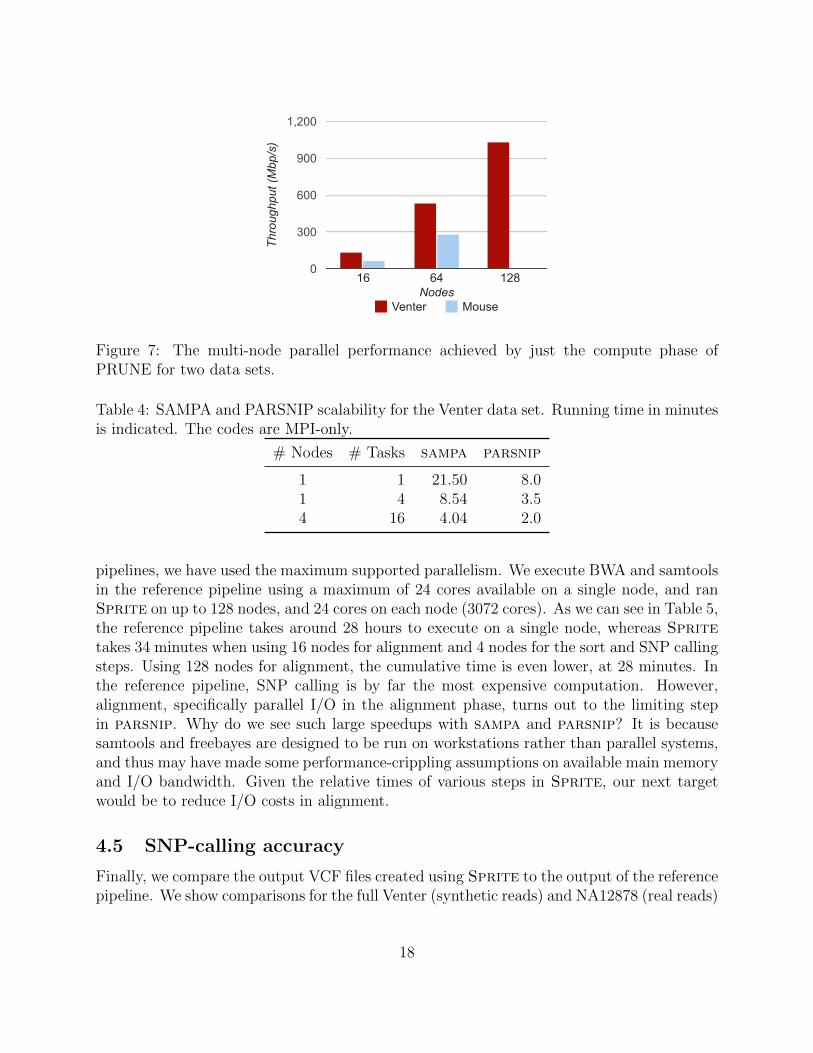
Table 4: SAMPA and PARSNIP scalability for the Venter data set. Running time in minutesis indicated. The codes are MPI-only.

# Nodes # Tasks sampa parsnip

1 1 21.50 8.01 4 8.54 3.54 16 4.04 2.0

pipelines, we have used the maximum supported parallelism. We execute BWA and samtoolsin the reference pipeline using a maximum of 24 cores available on a single node, and ranSprite on up to 128 nodes, and 24 cores on each node (3072 cores). As we can see in Table 5,the reference pipeline takes around 28 hours to execute on a single node, whereas Spritetakes 34 minutes when using 16 nodes for alignment and 4 nodes for the sort and SNP callingsteps. Using 128 nodes for alignment, the cumulative time is even lower, at 28 minutes. Inthe reference pipeline, SNP calling is by far the most expensive computation. However,alignment, specifically parallel I/O in the alignment phase, turns out to the limiting stepin parsnip. Why do we see such large speedups with sampa and parsnip? It is becausesamtools and freebayes are designed to be run on workstations rather than parallel systems,and thus may have made some performance-crippling assumptions on available main memoryand I/O bandwidth. Given the relative times of various steps in Sprite, our next targetwould be to reduce I/O costs in alignment.

4.5 SNP-calling accuracy

Finally, we compare the output VCF files created using Sprite to the output of the referencepipeline. We show comparisons for the full Venter (synthetic reads) and NA12878 (real reads)

18

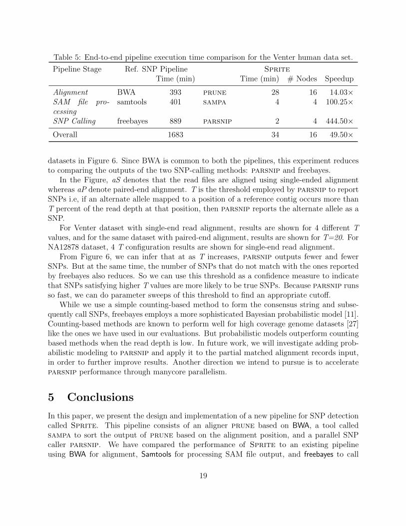
Table 5: End-to-end pipeline execution time comparison for the Venter human data set.

Pipeline Stage Ref. SNP Pipeline SpriteTime (min) Time (min) # Nodes Speedup

Alignment BWA 393 prune 28 16 14.03×SAM file pro-cessing

samtools 401 sampa 4 4 100.25×

SNP Calling freebayes 889 parsnip 2 4 444.50×

Overall 1683 34 16 49.50×

datasets in Figure 6. Since BWA is common to both the pipelines, this experiment reducesto comparing the outputs of the two SNP-calling methods: parsnip and freebayes.

In the Figure, aS denotes that the read files are aligned using single-ended alignmentwhereas aP denote paired-end alignment. T is the threshold employed by parsnip to reportSNPs i.e, if an alternate allele mapped to a position of a reference contig occurs more thanT percent of the read depth at that position, then parsnip reports the alternate allele as aSNP.

For Venter dataset with single-end read alignment, results are shown for 4 different Tvalues, and for the same dataset with paired-end alignment, results are shown for T=20. ForNA12878 dataset, 4 T configuration results are shown for single-end read alignment.

From Figure 6, we can infer that at as T increases, parsnip outputs fewer and fewerSNPs. But at the same time, the number of SNPs that do not match with the ones reportedby freebayes also reduces. So we can use this threshold as a confidence measure to indicatethat SNPs satisfying higher T values are more likely to be true SNPs. Because parsnip runsso fast, we can do parameter sweeps of this threshold to find an appropriate cutoff.

While we use a simple counting-based method to form the consensus string and subse-quently call SNPs, freebayes employs a more sophisticated Bayesian probabilistic model [11].Counting-based methods are known to perform well for high coverage genome datasets [27]like the ones we have used in our evaluations. But probabilistic models outperform countingbased methods when the read depth is low. In future work, we will investigate adding prob-abilistic modeling to parsnip and apply it to the partial matched alignment records input,in order to further improve results. Another direction we intend to pursue is to accelerateparsnip performance through manycore parallelism.

5 Conclusions

In this paper, we present the design and implementation of a new pipeline for SNP detectioncalled Sprite. This pipeline consists of an aligner prune based on BWA, a tool calledsampa to sort the output of prune based on the alignment position, and a parallel SNPcaller parsnip. We have compared the performance of Sprite to an existing pipelineusing BWA for alignment, Samtools for processing SAM file output, and freebayes to call

19

variants. Using 16 compute nodes with 24 cores each, Sprite completes in 34 minutes forthe Venter human data set, as compared to 28 hours taken by the existing pipeline’s singlenode execution. Also, the accuracy of SNPs reported by our variant calling step parsnipis comparable to the SNPs reported by freebayes. We will make our these tools publiclyavailable at our project website: sites.psu.edu/xpsgenomics.

Acknowledgments

This research is supported by the National Science Foundation award # 1439057. We thankmembers of our project research team, particularly Paul Medvedev and Mahmut Kandemir,for helpful discussions.

References

[1] D. Adjeroh, T. C. Bell, and A. Mukherjee. The Burrows-Wheeler Transform: DataCompression, Suffix Arrays, and Pattern Matching. Springer, 2008.

[2] S. F. Altschul, W. Gish, W. Miller, E. W. Myers, and D. J. Lipman. Basic localalignment search tool. Journal of molecular biology, 215(3):403–410, 1990.

[3] N. Axelrod, Y. Lin, P. C. Ng, T. B. Stockwell, J. Crabtree, J. Huang, E. Kirkness,R. L. Strausberg, M. E. Frazier, J. C. Venter, S. Kravitz, and S. Levy. The HuRefBrowser: a web resource for individual human genomics. Nucleic Acids Research,37(suppl 1):D1018–D1024, 2009.

[4] BMI OSU HPC Lab. pMap: Parallel sequence mapping tool. http://bmi.osu.edu/

hpc/software/pmap/pmap.html, last accessed April 2015.

[5] M. Burrows and D. J. Wheeler. A block sorting lossless data compression algorithm.Technical report 124. Technical report, Palo Alto, CA: Digital Equipment Corporation,1994.

[6] Convey ComputerTM

. TGAC speeds search with Convey. http://www.

conveycomputer.com/solutions/life-sciences/, last accessed April 2015.

[7] A. Darling, L. Carey, and W. Feng. The design, implementation, and evaluation ofmpiBLAST. In Proc. 4th Int’l. Conf. on Linux Clusters: The HPC Revolution 2003 inconjunction with ClusterWorld Conference and Expo, 2003.

[8] J. A. Edwards and U. Vishkin. Parallel algorithms for Burrows-Wheeler compressionand decompression. Theoretical Computer Science, 525:10–22, 2014.

[9] P. Ferragina and G. Manzini. Opportunistic data structures with applications. In Proc.Symp. on Foundations of Computer Science, pages 390–398, 2000.

20

[10] M. H. Y. Fritz, R. Leinonen, G. Cochrane, and E. Birney. Efficient storage of highthroughout DNA sequencing data using reference-based compression. Genome Research,21:734–740, 2011.

[11] E. Garrison and G. Marth. Haplotype-based variant detection from short-read sequenc-ing, 2012. http://arxiv.org/abs/1207.3907.

[12] A. Hatem, D. Bozdag, A. E. Toland, and U. V. Catalyurek. Benchmarking short se-quence mapping tools. BMC Bioinformatics, 14:184, 2013.

[13] W. J. Kent, C. W. Sugnet, T. S. Furey, K. M. Roskin, T. H. Pringle, A. M. Zahler, andD. Haussler. The human genome browser at UCSC. Genome research, 12(6):996–1006,2002.

[14] P. Klus, S. Lam, D. Lyberg, M. S. Cheung, G. Pullan, I. McFarlane, G. S. H. Yeo,and B. Y. H. Lam. BarraCUDA - a fast short read sequence aligner using graphicsprocessing units. BMC Research Notes, 5:27, 2012.

[15] B. Langmead and S. L. Salzberg. Fast gapped-read alignment with Bowtie 2. NatureMethods, 9(4):357–359, 2012.

[16] H. Li. Exploring single-sample SNP and INDEL calling with whole-genome de novoassembly. Bioinformatics, 28(14):1838–1844, 2012.

[17] H. Li and R. Durbin. Fast and accurate short read alignment with Burrows-Wheelertransform. Bioinformatics, 25(14):1754–1760, 2009.

[18] H. Li, B. Handsaker, A. Wysoker, T. Fennell, J. Ruan, N. Homer, G. Marth, G. Abeca-sis, R. Durbin, and 1000 Genome Project Data Processing Subgroup. The SequenceAlignment/Map format and SAMtools. Bioinformatics, 25(16):2078–2079, 2009.

[19] H. Li, J. Ruan, and R. Durbin. Mapping short dna sequencing reads and calling variantsusing mapping quality scores. Genome research, 18(11):1851–1858, 2008.

[20] R. Li, C. Yu, Y. Li, T.-W. Lam, S.-M. Yiu, K. Kristiansen, and J. Wang. SOAP2:an improved ultrafast tool for short read alignment. Bioinformatics, 25(15):1966–1967,2009.

[21] C. Liu, T. Wong, E. Wu, R. Luo1, S. Yiu, Y. Li, B. Wang, C. Yu, X. Chu, K. Zhao,R. Li, and T. Lam. SOAP3: ultra-fast GPU-based parallel alignment tool for shortreads. Bioinformatics, 28(6):878–879, 2012.

[22] Y. Liu and B. Schmidt. CUSHAW2-GPU: empowering faster gapped short-read align-ment using GPU computing. IEEE Design and Test, 31(1):31–39, 2014.

[23] Y. Liu, B. Schmidt, and D. L. Maskell. CUSHAW: a CUDA compatible short readaligner to large genomes based on the Burrows-Wheeler transform. Bioinformatics,28(14):1830–1837, 2012.

21

[24] H. Martınez, J. Tarraga, I. Medina, S. Barrachina, M. Castillo, J. Dopazo, and E. S.Quintana-Ortı. Concurrent and accurate RNA sequencing on multicore platforms. Tech-nical Report ICC 2013-03-01, Jaume I University, 2013.

[25] H. Martınez, J. Tarraga, I. Medina, S. Barrachina, M. Castillo, J. Dopazo, and E. S.Quintana-Ortı. A dynamic pipeline for RNA sequencing on multicore processors. InProc. European MPI Users’ Group Meeting (EuroMPI), pages 235–240, 2013.

[26] N. M. Mohamed, H. Lin, and W. Feng. Accelerating data-intensive genome analysis inthe cloud. In Proc. Int’l. Conf. on Bioinformatics and Computational Biology (BICoB),2013.

[27] R. Nielsen, J. S. Paul, A. Albrechtsen, and Y. S. Song. Genotype and SNP calling fromnext-generation sequencing data. Nat Rev Genet., 12(6):443–451, 2011.

[28] NVBIO library. https://github.com/NVlabs/nvbio, last accessed Apr 2015.

[29] SMaSH: A benchmarking toolkit for variant calling. http://http://smash.cs.

berkeley.edu/, last accessed April 2015.

[30] S. M. Rumble, P. Lacroute, A. V. Dalca, M. Fiume, A. Sidow, and M. Brudno. Shrimp:accurate mapping of short color-space reads. PLoS computational biology, 5(5):e1000386,2009.

[31] J. T. Simpson. Exploring genome characteristics and sequence quality without a refer-ence. arXiv preprint arXiv:1307.8026, 2013.

[32] J. T. Simpson and R. Durbin. Efficient construction of an assembly string graph usingthe FM-index. Bioinformatics, 26(12):367–373, 2010.

[33] J. T. Simpson and R. Durbin. Efficient de novo assembly of large genomes using com-pressed data structures. Genome Research, 22(3):549–556, 2012.

[34] A. Talwalkar, J. Liptrap, J. Newcomb, C. Hartl, J. Terhorst, K. Curtis, M. Bresler,Y. S. Song, M. I. Jordan, and D. Patterson. SMaSH: a benchmarking toolkit forhuman genome variant calling. Bioinformatics, 30(19):2787–2795, 2014.

[35] Y. Xin, B. Liu, B. Min, W. X. Y. Li, R. C. C. Cheung, A. S. Fong, and T. F. Chan. Par-allel architecture for DNA sequence inexact matching with Burrows-Wheeler Transform.Microlectronics Journal, 44(8):670–682, 2013.

[36] M. Zaharia, W. J. Bolosky, K. Curtis, A. Fox, D. Patterson, S. Shenker, I. Stoica, R. M.Karp, and T. Sittler. Faster and more accurate sequence alignment with SNAP, 2011.http://arxiv.org/abs/1111.5572, last accessed Apr 2015.

[37] J. Zhang, H. Lin, P. Balaji, and W. Feng. Optimizing Burrows-Wheeler Transform-based sequence alignment on multicore architectures. In Proc. IEEE/ACM Int’l. Symp.on Cluster, Cloud, and Grid Computing (CCGrid), pages 377–384, 2013.

22

[38] Y. Zhu, H. Jiang, X. Qin, and D. Swanson. A case study of parallel I/O for biologicalsequence search on Linux clusters. In Proc. IEEE Int’l. Conf. on Cluster Computing(Cluster), pages 308–315, 2003.

23