Journal of TurbulenceVol. 13, No. 38, 2012, 1–13

Energy exchange in an array of vertical-axis wind turbines

Matthias Kinzel∗, Quinn Mulligan and John O. Dabiri

Graduate Aeronautical Laboratories, California Institute of Technology, Pasadena, CA, USA

(Received 30 March 2012; final version received 7 July 2012)

We analyze the flow field within an array of 18 counter-rotating, vertical-axis wind tur-bines (VAWTs), with an emphasis on the fluxes of mean and turbulence kinetic energy.The turbine wakes and the recovery of the mean wind speed between the turbine rowsare derived from measurements of the velocity field using a portable meteorologicaltower with seven, vertically-staggered, three-component ultrasonic anemometers. Thedata provide insight to the blockage effect of both the individual turbine pairs withinthe array and the turbine array as a whole. The horizontal and planform kinetic energyfluxes into the turbine array are analyzed, and various models for the roughness lengthof the turbine array are compared. A high planform kinetic energy flux is measuredfor the VAWT array, which facilitates rapid flow recovery in the wake region behindthe turbine pairs. Flow velocities return to 95% of the upwind value within six rotordiameters downwind from each turbine pair. This is less than half the recovery dis-tance behind a typical horizontal-axis wind turbine (HAWT). The observed high levelof the planform kinetic energy flux is correlated with higher relative roughness lengthsfor the VAWT array as compared to HAWT farms. This result is especially relevantfor large wind farms with horizontal dimensions comparable to the height of the at-mospheric boundary layer. As shown in recent work and confirmed here, the planformkinetic energy flux can be the dominant source of energy in such large-scale wind farms.

Keywords: wind energy; energy transport; roughness length; turbulence

1. Introduction

The flow field in a wind farm is highly complex due to the interaction between the windturbines and the atmospheric boundary layer. While the fluid mechanics of individual windturbines are reasonably well understood, their performance is less predictable when situatedwithin a wind farm array. Due to aerodynamic interference between adjacent horizontal-axiswind turbines (HAWTs), in modern wind farms the HAWTs are typically spaced 3–5 rotordiameters, D, apart in the cross-wind direction and 6–10 D apart in the streamwise directionto achieve about 90% of the power output of an isolated HAWT [1, 2]. Recent researcheven suggests turbine spacings around 15 D for HAWT arrays based on an optimization ofthe costs per square rotor diameter [3].

To improve the understanding of wind farm aerodynamics, experimental studies haverecently been conducted in situ, e.g., at the Horns Rev wind farm in Denmark. In situmeasurements are challenging due to the large dimensions of the wind turbines and ofthe wind farm. The large spatial scales usually limit these investigations to pointwise

∗Corresponding author. Email: kinzel@caltech.edu

ISSN: 1468-5248 online onlyC© 2012 Taylor & Francis

http://dx.doi.org/10.1080/14685248.2012.712698http://www.tandfonline.com

Dow

nloa

ded

by [

Cal

ifor

nia

Inst

itute

of

Tec

hnol

ogy]

, [M

atth

ias

Kin

zel]

at 1

1:09

21

Sept

embe

r 20

12

2 M. Kinzel et al.

velocity measurements with meteorological towers, light detection and ranging (LIDAR),and satellite-based measurement techniques like synthetic aperture radar (SAR) and scat-terometry [4, 5]. However, these techniques can be sufficient to qualitatively characterizethe wake structures that are created by the individual wind turbines and the wind farm as awhole as well as the power drop between the turbine rows in the downwind direction. Scaledexperiments have been performed in wind tunnels for more detailed analyses, by usinglaboratory-based measurement techniques such as hot wire anemometry, laser Doppleranemometry (LDA), and particle image velocimetry (PIV; see, e.g., [6, 7]). Wind tunnel ex-periments have the limitation that it is usually not possible to simultaneously match both theReynolds numbers and the tip speed ratios (i.e., the ratio of blade tip speed to wind speed;TSRs) that occur in a real wind farm setting. Nevertheless they allow for important insightsinto these flows and are often used to validate numerical results from large eddy simulations(LES) [8, 9]. With the higher spatial resolutions of the wind tunnel experiments and thenumerical simulations, it is possible to access not only the flow velocities but also quantitieslike the Reynolds stresses, dispersive stresses, and fluxes and dissipation of kinetic energy.This data enables investigation of the mechanisms that deliver energy into the windfarm.

The power production of a wind turbine is determined by the kinetic energy flux of theair that moves through the rotor area,

Phorz = 0.5ρArotoru3, (1)

where ρ is the density of air, Arotor the area swept by the rotor, and u the horizontalwind velocity. If Arotor is replaced with the horizontal projected area of the wind farm,then Equation (1) describes the energy flux entering the wind farm from upwind. Thishorizontal kinetic energy flux is the dominant source of power for single turbines and smallwind farms [8]. For a large wind farm, however, the turbines in the rows located the furthestupwind deplete the horizontal energy flux before it reaches the majority of the turbines.Hence, in large wind farms where the length scale of the wind turbine array exceeds theheight of the atmospheric boundary layer (>1000 × 1000 m2), most of the turbines aresupplied by the planform energy flux through the top of the wind turbine array [8]. Theplanform flux of turbulence kinetic energy can be estimated as [7, 8],

Pvert ≈ −ρAplanu <u′w′>, (2)

where Aplan is the planform area above the wind turbine array and <u′w′> is the Reynoldsshear stress with turbulence velocities u′ and w′ in horizontal and vertical direction, re-spectively. Assuming a logarithmic wind velocity profile above the wind farm,

u(z) = u∗κ

[ln

(z − d

z0

)], (3)

the term − <u′w′> can be expressed as

− <u′w′>= u2∗ =

⎡⎣ uκ

ln(

z−dz0

)⎤⎦

2

. (4)

Dow

nloa

ded

by [

Cal

ifor

nia

Inst

itute

of

Tec

hnol

ogy]

, [M

atth

ias

Kin

zel]

at 1

1:09

21

Sept

embe

r 20

12

Journal of Turbulence 3

In this equation, u∗ is the friction velocity, κ the von Karman constant, κ ≈ 0.4, d thezero-plane displacement, which is often approximated by d ≈ 2H/3, and z0 the roughnesslength, which is often approximated by z0 ≈ H/10, where H is the turbine height (see [10]).Using typical values for current HAWTs of hub height H = 100 m and a flow velocity atthe hub height of u = 8 ms−1, the planform kinetic energy flux is approximately 70 Wm−2.

Rather than the rule of thumb z0 ≈ H/10, a more precise estimation of the roughnesslength of HAWT wind farms is often calculated with the Lettau formula [7, 8, 11]:

z0,Lett = 0.5h∗ s

S(5)

The Lettau roughness length depends on the height of the roughness elements, h∗, thefrontal area of the roughness elements, s, and the horizontal area per roughness element, S.For wind turbines, these values are usually chosen to be h∗ = H , s = Arotor, and S = sxsy ,where sx and sy are the dimensions of the horizontal area per wind turbine. For largeHAWTs, typical parameters are a hub height of 100 m, a rotor diameter of 130 m, and aturbine spacing of 10 D in streamwise and 5 D in the transversal direction. This leads toa roughness length of z0,Lett ≈ 1.5 m. In comparison, Frandsen [12] developed a formulaespecially for the calculation of the roughness length of HAWT wind farms:

z0,Fran = zh exp

[−

(8κ2sxsy

πCT

[1 − u2

∗lo

u2∗hi

])1/2]

(6)

Similar to the Lettau formula, the Frandsen formula also takes into account the turbine hubheight, zh = H , and horizontal area per turbine, sxsy , but adds turbine-specific parameters,i.e., the friction velocities at the top and bottom of the turbine rotor, u∗,hi and u∗,lo, and therotor thrust coefficient, CT = 4a(1 − a). Here, a = 0.5(1 − urear/ufront), where urear andufront are the averaged streamwise velocities downwind and upwind of the wind turbine.The performance of both the Lettau and Frandsen formulae will be evaluated for a VAWTarray in this paper.

Calaf et al. [8] report results for LES of a HAWT wind farm with dimensions thatscale to a hub height of 100 m, a rotor diameter of 100 m, and a wind farm area of1000 × 1000 m2. They simulated different turbine spacings and derived values for theroughness length between 0.41 m and 8.9 m depending on the geometrical and turbineparameters. The value that they calculated for a turbine spacing comparable to the one usedabove for the calculation of z0,Lett is 3.2 m. Inserting the Lettau and the numerically derivedroughness length into Equation (4) leads to a planform energy flux of about 21 Wm−2

and 37 Wm−2, respectively, smaller than that derived using the roughness length rule ofthumb z0 ≈ H/10. Considering the Betz limit (see, e.g., [2]), these values reduce to amaximum power production of approximately 12 Wm−2 and 22 Wm−2 for large windfarms. However, current wind farms have a typical power production of about 2.5 Wm−2,which is approximately a factor of seven smaller than these theoretical values [13]. This briefcalculation illustrates that, despite the power coefficients of modern HAWTs approachingthe Betz limit, there remains a significant gap between the performance of modern HAWTfarms as a whole and the theoretical upper bound given by the planform flux of kineticenergy that supplies the wind farm, the Betz limit notwithstanding.

As an alternative to HAWT farms for converting the planform kinetic energy flux toelectricity, here we study an array of counter-rotating VAWTs in a wind farm setting andcompare their performance to that of the conventional HAWTs. Previous work by [14, 15]

Dow

nloa

ded

by [

Cal

ifor

nia

Inst

itute

of

Tec

hnol

ogy]

, [M

atth

ias

Kin

zel]

at 1

1:09

21

Sept

embe

r 20

12

4 M. Kinzel et al.

suggests that wind farms consisting of closely spaced, counter-rotating VAWTs have thepotential to achieve an order of magnitude higher power production per unit footprint areathan the HAWT equivalent. This paper characterizes the energy transfer into an array of 18VAWTs, measures horizontal and planform kinetic energy flux, and compares and contraststhe results with conventional HAWT wind farms.

The turbine array and the experimental setup are discussed in the following section. InSection 3, the velocity field, velocity profiles, and energy transfer into the turbine array arepresented. Finally, in Section 4, the results are summarized and compared to the aforemen-tioned studies of HAWT wind farms in previous wind tunnel and LES investigations.

2. Methods

The VAWT array used in this study is located in the Antelope valley of northern LosAngeles County in California, USA. The location of the array is flat desert terrain for atleast 1.5 km in every direction. The mean horizontal wind speed during the measurementcampaign was 8.05 ms−1 at 10 m, i.e., just above the top of the wind turbine canopy, witha standard deviation of 2.1 ms−1. The prevailing wind direction is from the southwest.The probability density function (PDF) of the horizontal velocity during the time of themeasurements, 5 July–28 October 2011, is displayed in Figure 1(a) and the correspondingwind rose is given in Figure 1(b). The flow conditions were very similar between thedifferent days of the measurement campaign due to the desert climate. Wind speeds wouldusually exceed the cut-in speed of the turbines except for the early morning hours. Thereforemost of the measurements were taken at times when the atmospheric boundary layer is notneutrally stable, i.e., buoyancy effects contribute to the turbulence levels. The turbines area commercially available model (Windspire Energy Inc.) with a lift-based rotor designconsisting of three airfoils and a 1200-W generator that is connected to the base of theturbine shaft. The turbines have a total height of 9.1 m, a rotor height of 6.1 m, and adiameter of 1.2 m. The cut-in and cut-out speed of the wind turbines are 3.8 ms−1 and12 ms−1, respectively. The turbines operate at a nominal rotation rate of 350 rpm and aTSR of 2.3 at a typical inflow velocity of 8 ms−1. The turbine parameters are summarizedin Table 1.

The layout of the facility is shown in the photograph and sketch in Figures 2(a) and (b),respectively. The turbine array is comprised of a grid of nine counter-rotating turbine pairs

4 6 8 10 120.06

0.08

0.1

0.12

0.14

0.16

0.18

PD

F

uhor

[ms-1]

(a)

166h 333h

500h666h

N

S

EW

(b)

Figure 1. PDF of the horizontal velocity (a) and wind rose (b) for the time period of the measure-ments, 5 July–28 October 2011.

Dow

nloa

ded

by [

Cal

ifor

nia

Inst

itute

of

Tec

hnol

ogy]

, [M

atth

ias

Kin

zel]

at 1

1:09

21

Sept

embe

r 20

12

Journal of Turbulence 5

Table 1. Turbine parameters.

Height [m] Rotor height [m] D [m] sx [D] sy [D] ucut-in [ms−1] ucut-out [ms−1] rpm TSR

9.1 6.1 1.2 8 8 3.8 12 350 2.3

Figure 2. Photograph (a) and sketch (b) of the VAWT array. Blue circles symbolize clockwiserotating turbines and red circles symbolize anticlockwise rotating turbines. The axis dimensions aregiven in rotor diameters where D = 1.2 m. The tick marks on the abscissa indicate the measurementlocations.

Dow

nloa

ded

by [

Cal

ifor

nia

Inst

itute

of

Tec

hnol

ogy]

, [M

atth

ias

Kin

zel]

at 1

1:09

21

Sept

embe

r 20

12

6 M. Kinzel et al.

with the turbines in each counter-rotating pair 1.65 D apart from each other. The senseof rotation is such that the turbines rotate into the wind for the prevailing wind direction(see Figure 2(b)). The turbine pairs are arranged on an equidistant grid with distancessx = sy = 8 D = 9.6 m. This baseline configuration was derived from a systematic studyof the dependency of the power production of VAWTs on the layout of the turbine locationsand the wind direction by [14].

The vertical velocity profiles of the flow were measured at 11 positions along the centerline of the turbine array as shown in Figure 2(b). The measurement positions are indicatedon the abscissa. For these measurements, seven three-component ultrasonic anemometers(Campbell Scientific CSAT3) were mounted on one 10-m meteorological tower (Aluma-Towers Inc.) and vertically spaced in 1-m increments over the turbine rotor height. Fig-ure 3(a) shows the ultrasonic anemometers mounted to the met tower and their positioningwith respect to the turbine rotors. A detailed picture of one of the sensors with the threesensor head pairs visible is shown in Figure 3(b). The CSAT3 sensors were operated ata sampling frequency (fsample) of 10 Hz with a measurement uncertainty of less than0.161 ms−1. Both the sensors and the data logger (Campbell Scientific CR3000) were pow-ered by a solar panel and battery system to make the apparatus fully portable. The tower wasmoved consecutively to each measurement position along the center line of the turbine array(see measurement transect in Figure 2(b)). The measurement duration at each position wasapproximately 150 h. This time interval was sufficiently long so as to obtain statisticallyindependent data for the values of the mean and fluctuating velocities.

Because the velocities at the 11 tower positions were not measured simultaneously, thewind speed information from a 10-m reference meteorological tower at the southeast cornerof the turbine array was used to condition the data (Figure 2(b)). This anemometer (ThiesFirst Class) recorded data at 1 Hz with an accuracy of ±3%. Using the reference winddata, the measurements from the seven ultrasonic sensors were divided into 10-min timeintervals and sorted into bins between 4−6 ms−1, 6−8 ms−1, 8−10 ms−1, and 10−12 ms−1

Figure 3. Photograph of a turbine pair with the seven CSAT3 sensors in the background (a) and ofone CSAT3 sensor (b). The met-tower for the sensors can be made out behind the left turbine.

Dow

nloa

ded

by [

Cal

ifor

nia

Inst

itute

of

Tec

hnol

ogy]

, [M

atth

ias

Kin

zel]

at 1

1:09

21

Sept

embe

r 20

12

Journal of Turbulence 7

Table 2. Measurement parameters.

Measurement Measurement Durationfsample [Hz] uncertainty [ms−1] period per location [h]

10 0.161 5 July–28 October 2011 ≈150

depending on the mean velocity information from the reference anemometer. The lower(4 ms−1) and upper bound (12 ms−1) were chosen to coincide with the cut-in and cut-outspeeds of the turbines. Table 2 lists the measurement parameters.

3. Results

Averaging the velocities over the seven sensor positions at each measurement locationyields the average mean horizontal flow velocity at the rotor midheight. The curve for theaveraged mean horizontal flow velocity along the center line of the turbine array is plottedin Figure 4. The measurement transect is plotted on the abscissa and the average of thehorizontal velocity over the rotor height on the ordinate. The three turbine pairs along thecenter line of the turbine array are sketched as vertical bars in the figure at 0 D, 11 D, and22 D. The error bars show the standard deviation, which is indicative of the turbulencefluctuations at each measurement position. The standard deviation was calculated from allinstantaneous velocity measurements. The first measurement point is located 15 D upwindof the wind turbine array where the flow is undisturbed by the presence of the turbines.From this free stream horizontal velocity of 7.2 ms−1, the flow slows down to 6.5 ms−1 atthe position 1.5 D in front of the first turbine pair. This illustrates the blockage effect thatthe turbine array has on the flow. From the second to the third data point, the velocity dropsto 5.1 ms−1 over the first turbine pair as the turbines extract energy from the flow. Thisvelocity drop is followed by a recovery to 6.3 ms−1 as energy is brought into the turbinearray from above and the sides. The energy extraction and recovery cycle repeats itselffor the second and third turbine pairs. The velocity to which the flow recovers is lower

−20 −10 0 10 20 30 400

0.2

0.4

0.6

0.8

1

1.2

u hor /

U∞

x/D

Figure 4. Average mean horizontal flow velocity at rotor midheight normalized by the inflow velocityas measured by the reference anemometer at 10 m plotted over the measurement transect. The threeturbine pairs are sketched as vertical bars. The error bars indicate the standard deviation.

Dow

nloa

ded

by [

Cal

ifor

nia

Inst

itute

of

Tec

hnol

ogy]

, [M

atth

ias

Kin

zel]

at 1

1:09

21

Sept

embe

r 20

12

8 M. Kinzel et al.

Figure 5. Normalized horizontal velocity contours along the center of the turbine array. The threeturbine pairs are indicated by vertical bars.

for the second turbine pair (5.9 ms−1) than for the first but stays approximately the samebetween the second and the third turbine pairs (6.0 ms−1). The distance behind a turbinepair required for the flow to recover to 95% of the wind velocity in front of the turbine pair isapproximately 6 D. This is larger than the distance of 4 D that was observed by [14], albeitfor the wake behind a single VAWT. It is significantly smaller than the 14 D that the flowbehind a typical HAWT requires to recover to 95% of the upwind velocity (see [16]). Afterthe third turbine pair, the curve shows the recovery of the flow up to a point 15 D downwindof the turbine array where the horizontal flow velocity is still lower than at the point 1.5 Din front of the turbine array. The two measurement points 3 D and 1.5 D in front of the thirdturbine pair show how the velocity decreases in front of the turbine pair, which indicates theblockage effect that the individual turbine pairs create in the flow. Therefore, the recoveryregion does not cover the whole area between two turbine pairs but starts right behind theupwind turbine pair and ends approximately 2 D in front of the downwind turbine pair.

When the data from the seven sensors and the 11 measurement locations are combined,the two-dimensional flow field along the center line of the turbine array is revealed. Thenormalized horizontal velocities of this flow field are depicted in Figure 5. The measurementtransect is presented on the abscissa, the vertical direction on the ordinate, and the horizontalvelocity is given as a contour plot. Again, the three turbine pairs are indicated by the blackvertical bars at 0 D, 11 D, and 22 D. The two-dimensional horizontal velocity field revealsdetails regarding the flow around the VAWTs. The highest flow velocities can be found atthe top of the wind turbine array as expected. Also, the wake and recovery regions canbe clearly made out for the three different turbine pairs. The contours show that the flowvelocities drop over the area where the turbine pairs are located as energy is extracted fromthe flow. Subsequently, the flow velocities start to increase again before the flow interactswith the next turbine pair. The increase in the flow velocities is highest close to the topof the turbines but the recovery is also faster at the bottom of the rotors than at midspan.There is a slight difference in the turbine wake region between the three rows of turbines.The flow velocities remain relatively high after the first row of turbines because the energytransfer from the front and the sides is still dominant in this region of the turbine array. Afaster flow recovery can also be seen behind the last row of turbines where there are noturbines located behind or to the sides of the turbine pair. The effect of the absent turbines

Dow

nloa

ded

by [

Cal

ifor

nia

Inst

itute

of

Tec

hnol

ogy]

, [M

atth

ias

Kin

zel]

at 1

1:09

21

Sept

embe

r 20

12

Journal of Turbulence 9

(a) (b)

Figure 6. (a) Profiles of the horizontal flow velocity between 0 < z < 40 D at 15 D (solid) and 1.5 D(dash) upwind and 2 D (dash-dot) and 15 D (dot) downwind of the turbine array. The measurementpoints are given by markers. (b) Profiles of the horizontal flow velocity over the rotor height 1.5 D(solid) upwind, 2 D (dash), 4 D (dash-dot), and 7.5 D (dash-dot) downwind of the third turbine pair.

behind the last turbine pair becomes most obvious near the top of the wind turbines forx > 29 D. However, the flow velocities remain significantly lower behind the turbine arraythan in the same distance upwind of the turbine array.

The interaction between the turbine array and the atmospheric boundary layer is illus-trated in Figure 6(a). The velocity profiles at 15 D (solid line) and 1.5 D (dashed line) upwindof the turbine array as well as 2 D (dash-dotted line) and 15 D (dotted line) downwind of theturbine array are plotted over the vertical distance from the ground. The data on the abscissais plotted logarithmically. The velocity profile of the atmospheric boundary layer upwindof the turbine array is extrapolated below and above the rotor area with the assumption of alogarithmic profile (see Equation (3)). The estimates d = 2/3H and z0 = H/10 were usedto calculate the zero plane displacement and roughness length. For H, the average length ofthe ground vegetation of 0.1 m was applied. The measurement points are given by markerswhile the interpolated part of the curve does not contain markers. The measurement pointsfit very well on the curve for the velocity profile of a logarithmic boundary layer. Theblockage effect of the turbine array is clearly visible at the measurement location 1.5 D infront of the turbine array. Here, the flow velocities are on average 10% lower in the regionof the turbine rotors than they are for the undisturbed velocity profile 15 D upwind of thearray. The largest deviation from the undisturbed profile is close to the rotor midspan. Thisblockage effect is significantly larger for the densely spaced VAWT array than for HAWTwind farms (compare, e.g., [8]). The turbine signature in the horizontal flow velocity profileis more significant at the measurement location 2 D downwind of the turbine array. Theflow velocities are about 32% lower compared to the measurement location 1.5 D upwindof the turbine array. The velocity profile 15 D downwind of the turbine array shows therecovery of the flow velocities in the wake of the turbine array. However, the flow velocitiesonly recover to a value of 86% of the flow velocities 15 D upwind of the turbine array andeven stay 4% below the flow velocities at the position 1.5 D in front of the turbine array.

Profiles of the horizontal flow velocities over the rotor height are plotted in Figure 6(b)for the measurement positions in the proximity of the third turbine pair. These curves allowanalysis of the extraction of energy by the turbine pair as well as the recovery of the flowvelocities in the turbine pair’s wake. The measurement locations are 1.5 D upwind and 2 D,

Dow

nloa

ded

by [

Cal

ifor

nia

Inst

itute

of

Tec

hnol

ogy]

, [M

atth

ias

Kin

zel]

at 1

1:09

21

Sept

embe

r 20

12

10 M. Kinzel et al.

4 D, and 7.5 D downwind of the turbine pair. The velocity profiles are presented for thethird turbine pair because the most measurement positions are available here. However,the corresponding curves for the second turbine pair are qualitatively similar and varyquantitatively by less than 12.5%. A typical wind profile for the flow in the interior ofthe wind farm is represented by the velocity profile 1.5 D upwind of the third turbine pair(solid line). The lowest velocity at this location is 5.3 ms−1 and can be found at a positionaround 1/3H from the bottom of the rotor. From there the velocities monotonically increasetoward the top and the bottom of the rotor. The velocities are significantly higher at thetop than at the bottom of the rotor with values of 7.0 ms−1 and 5.8 ms−1 respectively.The overall velocity profile is due to the higher flow velocities mainly above the turbinecanopy but also below the rotor. Energy is transferred from these outer regions into the areaof the turbine rotors. The flow is more energetic above the turbine canopy, which resultsin the higher flow velocities in the upper regions of the rotors. The flow velocities dropon average 1.4 ms−1 to the next measurement position 2 D downwind of the turbine pair.This drop in velocity is equivalent to a loss of kinetic energy and a power extraction fromthe flow of approximately 1.0 kW based on the frontal area of a turbine pair of VAWTsA2rotors = 14.6 m2 (see Equation (1)). The power density based on the planform area perturbine pair is 11.0 Wm−2. The flow then recovers 0.6 ms−1 on average between 2 D and4 D and 1 ms−1 between 4 D and 7.5 D behind the turbine pair. This is equivalent to apower recovery of 12.7 Wm−2 based on the planar area of one turbine pair, which providesslightly more energy than the turbine pair extracts. Again, the velocity profiles show therecovery of the flow to a value close to the upwind flow velocity within approximately 6 D.

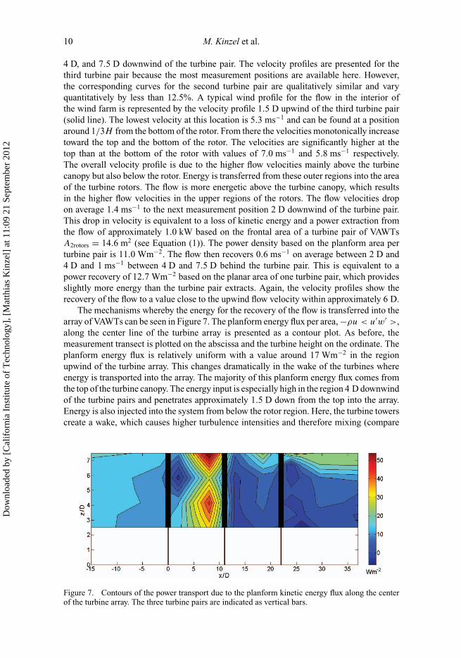
The mechanisms whereby the energy for the recovery of the flow is transferred into thearray of VAWTs can be seen in Figure 7. The planform energy flux per area, −ρu < u′w′ >,along the center line of the turbine array is presented as a contour plot. As before, themeasurement transect is plotted on the abscissa and the turbine height on the ordinate. Theplanform energy flux is relatively uniform with a value around 17 Wm−2 in the regionupwind of the turbine array. This changes dramatically in the wake of the turbines whereenergy is transported into the array. The majority of this planform energy flux comes fromthe top of the turbine canopy. The energy input is especially high in the region 4 D downwindof the turbine pairs and penetrates approximately 1.5 D down from the top into the array.Energy is also injected into the system from below the rotor region. Here, the turbine towerscreate a wake, which causes higher turbulence intensities and therefore mixing (compare

Figure 7. Contours of the power transport due to the planform kinetic energy flux along the centerof the turbine array. The three turbine pairs are indicated as vertical bars.

Dow

nloa

ded

by [

Cal

ifor

nia

Inst

itute

of

Tec

hnol

ogy]

, [M

atth

ias

Kin

zel]

at 1

1:09

21

Sept

embe

r 20

12

Journal of Turbulence 11

Figure 8. Contours of the turbulence intensity along the center of the turbine array. The three turbinepairs are sketched as vertical structures.

Figure 8). However, this energy transfer is 0.4 Wm−2 on average, which is two ordersof magnitude smaller than the one from above the turbine array. Also, its contributionto the total energy flux into the rotor region decreases with increasing size of the windfarm area because the energy below the rotor canopy gets depleted by the turbines locatedfurther upwind and does not reach the majority of turbines in the center of large arrays.The regions of high energy transfer agree with the regions of high horizontal velocity inFigure 5. The region behind the first turbine pair stands out because the Reynolds shearstress is a factor of two higher than in the corresponding regions behind the second andthird turbine pairs. This indicates a higher level of turbulence in the wake of the first turbinepair in comparison to the other two turbine pairs. This is caused by the interaction of thefirst turbine pair, which stands exposed in the front of the turbine array and the atmosphericboundary layer. Averaging the planform energy flux for the highest sensor position from2 D downwind of the second turbine pair to 7.5 D downwind of the third turbine pairresults in an average kinetic energy flux into the turbine array of 22 Wm−2. A separate setof measurements collected 0.8 D away from the symmetry axis of the VAWT array showthat the energy flux is relatively homogeneous in the region where the turbines are located.But it is to be expected that the turbulence intensity and therefore the planform energy fluxare slightly lower in the regions along the lines where the wind does not interact directlywith the turbines. However, these regions constitute only 3.8% of the total wind farm area.Therefore, a constant value is assumed for the planform energy flux. With the planformarea of 8 × 8 D per turbine pair, this leads to a vertical power input of 2.1 kW. This meansthat the 1.0 kW, which were shown to be extracted by one turbine pair, can be suppliedcompletely by the planform energy flux.

The turbulence intensity along the center of the turbine array is shown as a contour plotin Figure 8. As mentioned above the turbulence intensity is the highest in the turbine wakeswith the maximum right behind the rotor.

The roughness length can be estimated by different models, which in turn has aninfluence on the estimate of the planform energy flux. When the roughness length isestimated by z0 ≈ H/10 = 0.91 m, Equation (2) results in a planform energy flux of42 Wm−2. The values of the roughness length as calculated by the Lettau and Frandsenformulae, Equations (5) and (6), are 0.72 m and 0.13 m, respectively. These formulae leadto a the planform energy flux of 29 Wm−2 and 6 Wm−2 respectively. While the value for the

Dow

nloa

ded

by [

Cal

ifor

nia

Inst

itute

of

Tec

hnol

ogy]

, [M

atth

ias

Kin

zel]

at 1

1:09

21

Sept

embe

r 20

12

12 M. Kinzel et al.

Table 3. Roughness lengths and vertical energy flux for VAWT and HAWT [4, 8] arrays.

< uhor > uhor’ z0,Lett z0,Fran Pz0 Pz0,Lett/from Pz0,Fran Pmeasured

[ms−1] [ms−1] z0 [m] [m] [m] [Wm−2] LES [Wm−2] [Wm−2] [Wm−2]

VAWT array 8.05 2.1 0.91 0.72 0.13 42 29 6 24HAWT array 8.4 10 1.5 3.2 71 21 37 2.5

planform energy flux as calculated by the Lettau formula lies within 30% of the measuredvalue, the respective values from the estimation and the Frandsen formulae are off by 90%and 75%. These values are summarized in Table 3 and compared to the correspondingvalues for HAWT arrays.

The total energy that is available inside the wind farm is the sum of the planform energyflux and the power that is transferred into the wind farm from the sides. Taking the windvelocities at the measurement position 1.5 D in front of the first turbine pair as inflowconditions and assuming a logarithmic velocity profile for the area underneath the rotorsleads to a horizontal energy flux of 106 Wm−2 (see Equation (1)). This is approximately fivetimes the power available from the planform energy flux. With the frontal area per turbinepair of 8 × 7.5 D, this results in a horizontal power transport of 9.2 kW. Only 0.76 kW ofthis energy is located in the region below the turbine rotor, which supports that this regionis less significant for the total energy transfer into the turbine array.

4. Conclusions

This experimental field study has analyzed the flow field along the center line of an arrayof nine pairs of full-scale counter-rotating VAWTs. The velocity field shows the blockageeffect of the turbine array as well as the blockage effect of the individual turbine pairswithin the array.

The distance behind a turbine pair that the flow needs to recover to 95% of the windvelocity upwind of the turbine pair is approximately 6 D. In comparison, a recovery distanceof 4 D was observed by [14] for the wake behind a single VAWT. The distance requiredfor a recovery of the flow velocities is significantly smaller than the 14 D that the flowbehind HAWTs needs to recover to 95% of the upwind velocity (see [16]). Hence, pairingthe VAWTs may lead to an overall reduction in the average inter-turbine spacing in windfarm arrays.

The horizontal energy flux from the sides is approximately five times higher thanthe planform energy flux through the top of the turbine canopy. Nevertheless, the planformkinetic energy flux is approximately 15% larger than the energy that the turbines extract fromthe flow, indicating that it is sufficient to supply energy to the turbines. This is important forlarge wind farms where the horizontal dimensions exceed that of the atmospheric boundarylayer height. The horizontal energy flux will be depleted before it reaches the majority ofthe turbines in those cases, leaving the planform energy flux as the primary power source.The high planform energy flux in the VAWT array also appears to enable the flow torecover quickly in the wake region behind the turbine pairs. One possible explanation forthe relatively high planform kinetic energy flux may be the elevated level of turbulence,which is higher close to the ground than in the regions above where the HAWTs operate.Also, the roughness length of the VAWTs appears to have a stronger influence on the flow,

Dow

nloa

ded

by [

Cal

ifor

nia

Inst

itute

of

Tec

hnol

ogy]

, [M

atth

ias

Kin

zel]

at 1

1:09

21

Sept

embe

r 20

12

Journal of Turbulence 13

i.e., increasing the planform energy flux into the turbine array. The roughness length relativeto turbine height was observed to be larger for the VAWTs than for typical HAWTs.

The data suggest that the Frandsen formula, which was developed to calculate theroughness length for HAWT wind farms, does not give a good estimate for a VAWT windfarm. The result for the roughness length obtained with the Lettau formula appears to be inbetter agreement with measurement data. However, the development of a roughness lengthformula specifically for VAWT arrays is desirable.

The results presented in this paper are dependent on several variables that were notinvestigated presently, including the turbine spacing and rotational sense, and the specificsof the VAWT design, such as rotor solidity, TSR, thrust coefficient, etc. Ongoing and futurework is directed toward determining the dependence of energy exchange on these additionalparameters.

Acknowledgments

The authors gratefully acknowledge funding from the National Science Foundation Energyfor Sustainability program (Grant No. CBET-0725164) and the Gordon and Betty MooreFoundation.

References[1] B. Sørensen, Renewable Energy: Its Physics, Engineering, Use, Environmental Impacts, Econ-

omy, and Planning Aspects, Elsevier, London, 2004.[2] E. Hau, Wind Turbines, Springer-Verlag, Berlin, 2006.[3] M. Meyers and C. Meneveau, Optimal turbine spacing in fully developed wind farm boundary

layers, Wind Energy 15 (2012), pp. 305–317.[4] C.B. Hasager, R.J. Barthelmie, M.B. Christiansen, M. Nielsen, and S.C. Pryor, Quantifying

offshore wind resources from satellite wind maps: Study area the North Sea, Wind Energy 9(2006), pp. 63–74.

[5] M. Mechali, R. Barthelmie, S. Frandsen, L. Jensen, and P.E. Rethore, Wake effects at Horns Revand their influence on energy production, European Wind Energy Conference and Exhibition,Athens, Greece, 2006.

[6] L.P. Chamorro, R.E.A. Arndt, and F. Sotiropoulos, Turbulent flow properties around a staggeredwind farm, Bound.-Layer Meteorol. 141 (2011), pp. 349–367.

[7] R.B. Cal, J. Lebron, L. Castillo, H.S. Kang, and C. Meneveau, Experimental study of thehorizontally averaged flow structure in a model wind-turbine array boundary layer, Renew.Sust. Energy 2 (2010), 013106.

[8] M. Calaf, C. Meneveau, and J. Meyers, Large eddy simulation study of fully developed wind-turbine array boundary layers, Phys. Fluids 22 (2010), 015110.

[9] L.P. Chamorro and F. Porte-Agel, A wind-tunnel investigation of wind-turbine wakes: Boundary-layer turbulence effects, Bound.-Layer Meteorol. 132 (2009), pp. 129–149.

[10] J.R. Garratt, The Atmospheric Boundary Layer, Cambridge University Press, Cambridge, 1994.[11] H. Lettau, Note on aerodynamic roughness-parameter estimation on the basis of roughness-

element description, J. Appl. Meteorol. 8 (1969), pp. 828–832.[12] S. Frandsen, On the wind speed reduction in the center of large clusters of wind turbines,

J. Wind Eng. Ind. Aerodyn. 39 (1992), pp. 251–265.[13] D.J.C. MacKay, Sustainable Energy – Without the Hot Air, UIT Cambridge, Cambridge, 2009.[14] J.O. Dabiri, Potential order-of-magnitude enhancement of wind farm power density via counter-

rotating vertical-axis wind turbine arrays, J. Renew. Sust. Energy 3 (2011), 043104.[15] R.W. Whittlesey, S. Liska, and J.O. Dabiri, Fish schooling as a basis for vertical axis wind

turbine farm design, Bioinsp. Biomim. 5 (2010), 035005.[16] N. Kelley and B. Jonkman, A stochastic, full-field, turbulent-wind simulator for use with

the AeroDyn-based design codes, online database (2009). Available at http://wind.nrel.gov/designcodes/preprocessors/turbsim/.

Dow

nloa

ded

by [

Cal

ifor

nia

Inst

itute

of

Tec

hnol

ogy]

, [M

atth

ias

Kin

zel]

at 1

1:09

21

Sept

embe

r 20

12