endogenous growth sophia kazinnik university of houston economics department

Endogenous growth

Sophia Kazinnik

University of Houston Economics Department

A bit of background:

• The neoclassical growth model that we studies previously (Solow-Swan) provides important insights about growth, but also has serious limitations.

• One of the limitations is that the long run rate of growth is determined outside of the model - exogenously.

• As we have seen before, in neoclassical growth model, the steady state rate of growth will be driven by the rate of technological progress.

• But what if we want to know what drives technological progress itself?

Neoclassical Growth Model vs. “New Growth Theory”

2

• A “new growth theory” (endogenous growth) was developed to

extend neoclassical growth theory (exogenous growth). It extends

the neoclassical growth model to allow for endogenously driven

growth (Romer, Lucas).

• Today we will look at couple of core models underlying this

research.

3

Neoclassical Growth Model vs. “New Growth Theory”

4

AK model - preliminaries

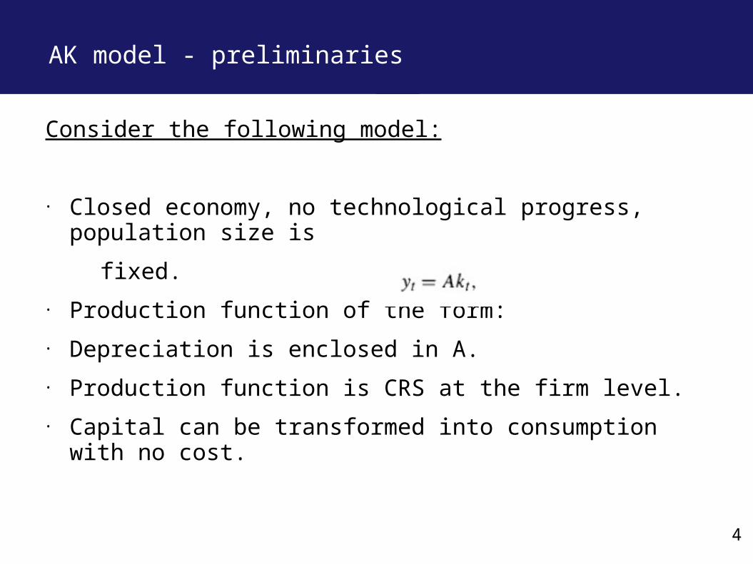
Consider the following model:

• Closed economy, no technological progress, population size is

fixed.

• Production function of the form:

• Depreciation is enclosed in A.

• Production function is CRS at the firm level.

• Capital can be transformed into consumption with no cost.

4

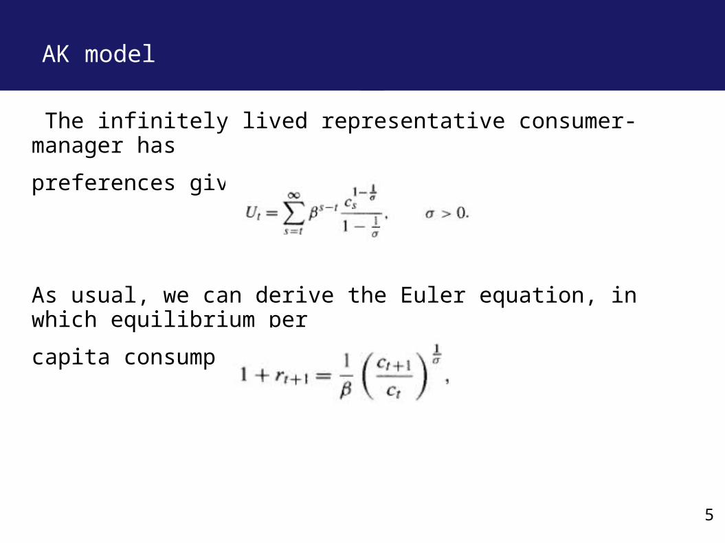
The infinitely lived representative consumer-manager has

preferences given by:

As usual, we can derive the Euler equation, in which equilibrium per

capita consumption obeys:

Now lets determine the equilibrium in this model. 5

AK model

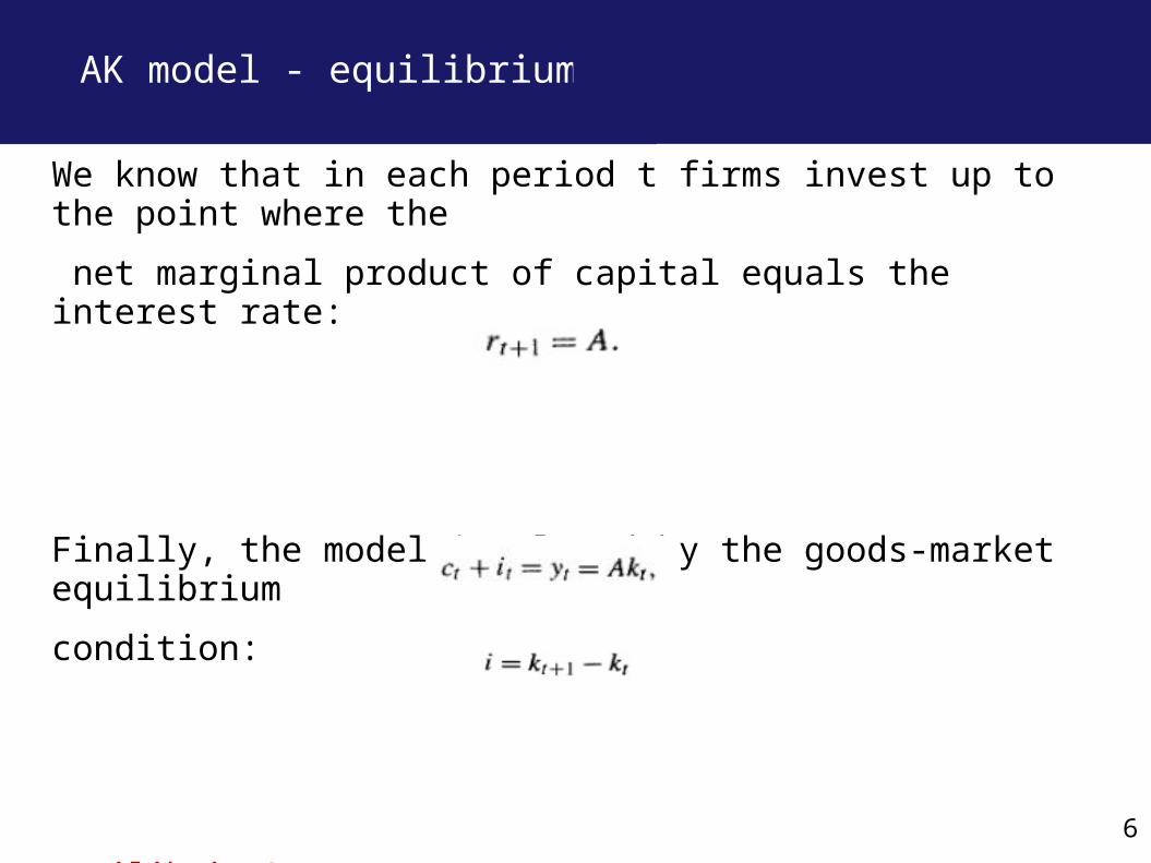
We know that in each period t firms invest up to the point where the

net marginal product of capital equals the interest rate:

Finally, the model is closed by the goods-market equilibrium

condition:

Equilibrium?

6

AK model - equilibrium

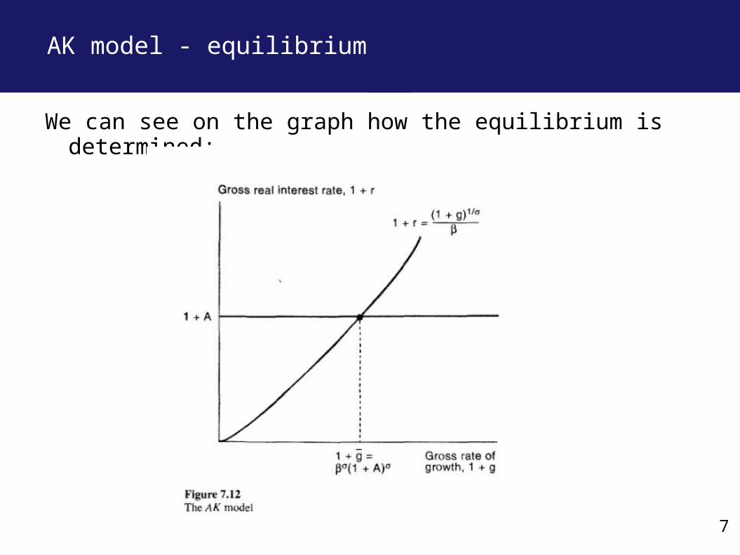
We can see on the graph how the equilibrium is determined:

7

AK model - equilibrium

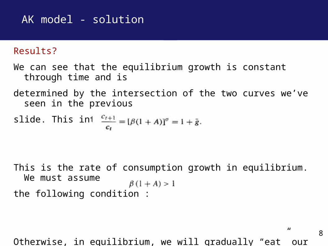
Results?

We can see that the equilibrium growth is constant through time and is

determined by the intersection of the two curves we’ve seen in the previous

slide. This intersection yields:

This is the rate of consumption growth in equilibrium. We must assume

the following condition :

Otherwise, in equilibrium, we will gradually “eat” our capital away.

8

AK model - solution

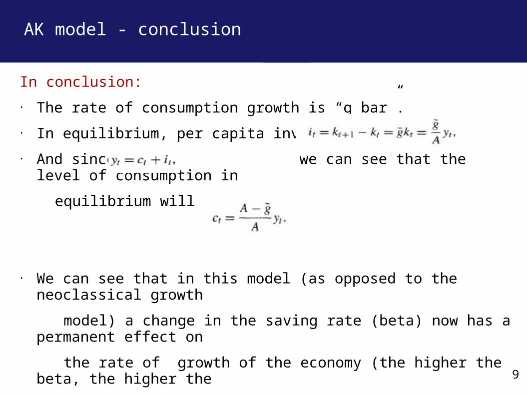
In conclusion:

• The rate of consumption growth is “g bar”.

• In equilibrium, per capita investment is:

• And since we can see that the level of consumption in

equilibrium will be:

• We can see that in this model (as opposed to the neoclassical growth

model) a change in the saving rate (beta) now has a permanent effect on

the rate of growth of the economy (the higher the beta, the higher the

growth rate).9

AK model - conclusion

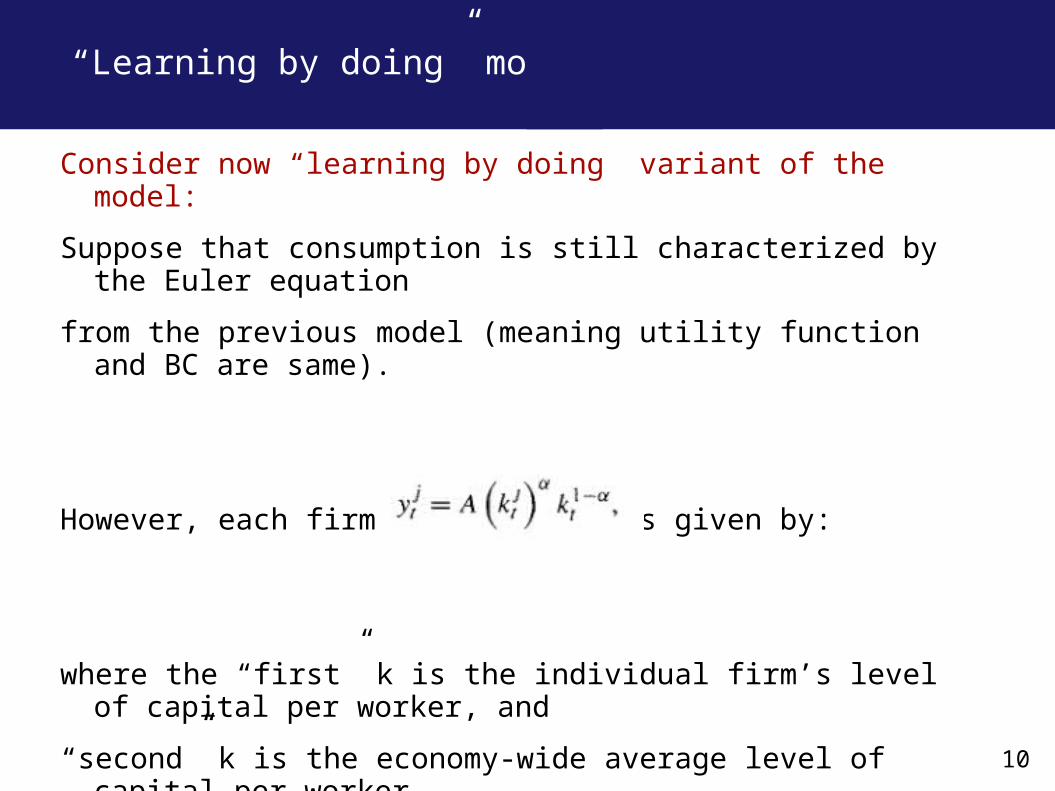
Consider now “learning by doing” variant of the model:

Suppose that consumption is still characterized by the Euler equation

from the previous model (meaning utility function and BC are same).

However, each firm’s j’s output is given by:

where the “first” k is the individual firm’s level of capital per worker, and

“second” k is the economy-wide average level of capital per worker.

10

“Learning by doing” model

11


11

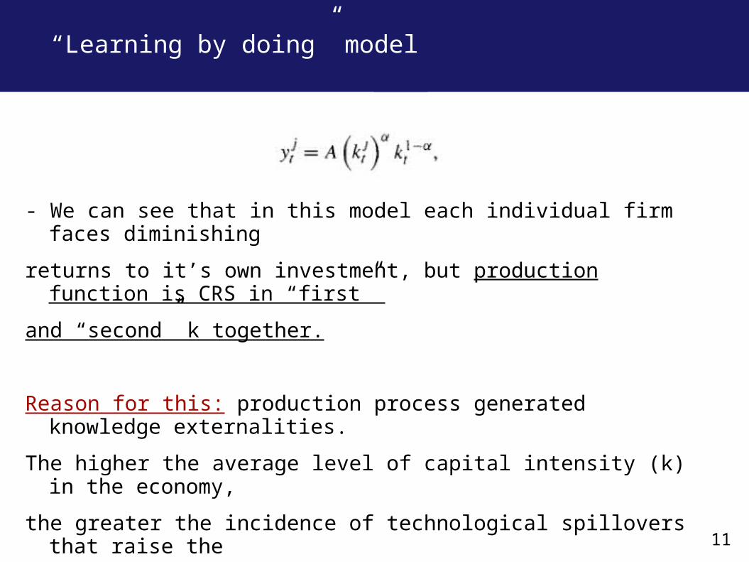
- We can see that in this model each individual firm faces diminishing

returns to it’s own investment, but production function is CRS in “first”

and “second” k together.

Reason for this: production process generated knowledge externalities.

The higher the average level of capital intensity (k) in the economy,

the greater the incidence of technological spillovers that raise the

marginal productivity of capital throughout the economy.

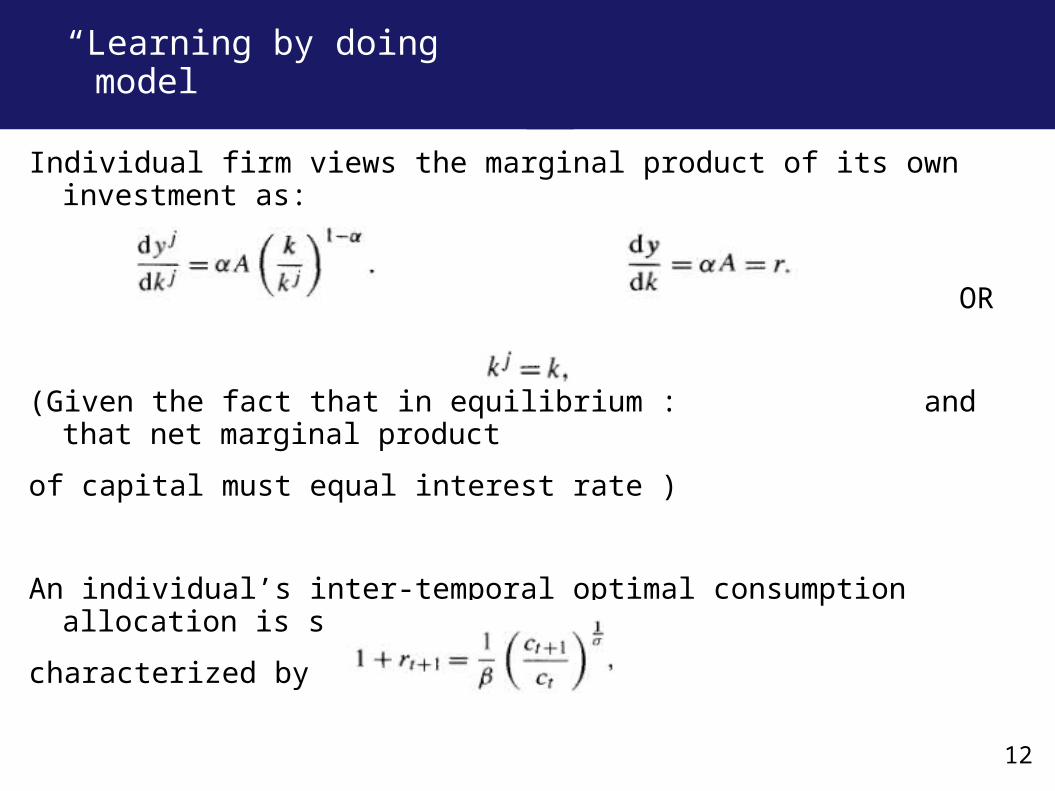
Individual firm views the marginal product of its own investment as:

OR

(Given the fact that in equilibrium : and that net marginal product

of capital must equal interest rate )

An individual’s inter-temporal optimal consumption allocation is still

characterized by the Euler equation:

Equilibrium?

12


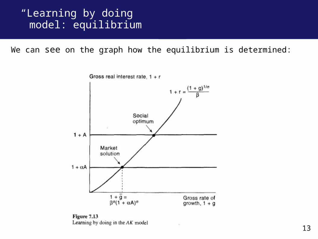
We can see on the graph how the equilibrium is determined:

13

“Learning by doing” model: equilibrium

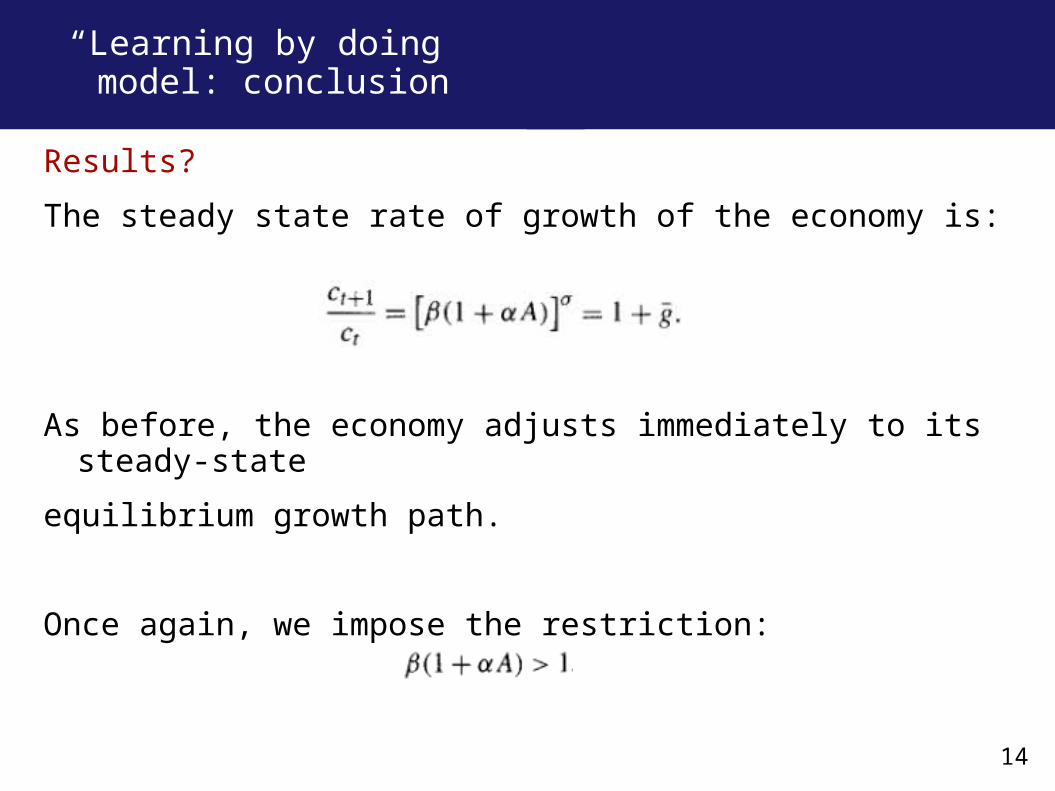
Results?

The steady state rate of growth of the economy is:

As before, the economy adjusts immediately to its steady-state

equilibrium growth path.

Once again, we impose the restriction:

14

“Learning by doing” model: conclusion

15

AK vs. “learning by doing”

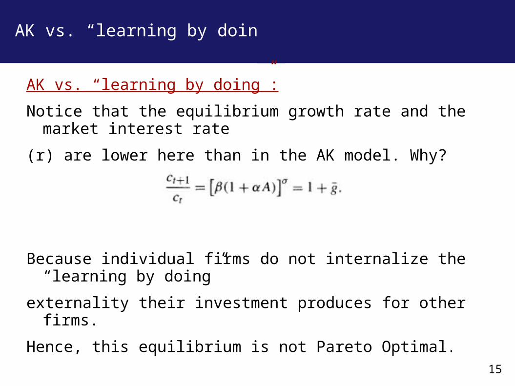
AK vs. “learning by doing”:

Notice that the equilibrium growth rate and the market interest rate

(r) are lower here than in the AK model. Why?

Because individual firms do not internalize the “learning by doing”

externality their investment produces for other firms.

Hence, this equilibrium is not Pareto Optimal.

15

International capital market integration can raise the level of world

output by allowing capital to migrate toward its most productive global

uses.

Here, we will use a stochastic version of the AK model to illustrate how

world capital market integration can raise steady-state growth.

We will start with the closed economy in investment autarky.

16

International Capital Market Integration

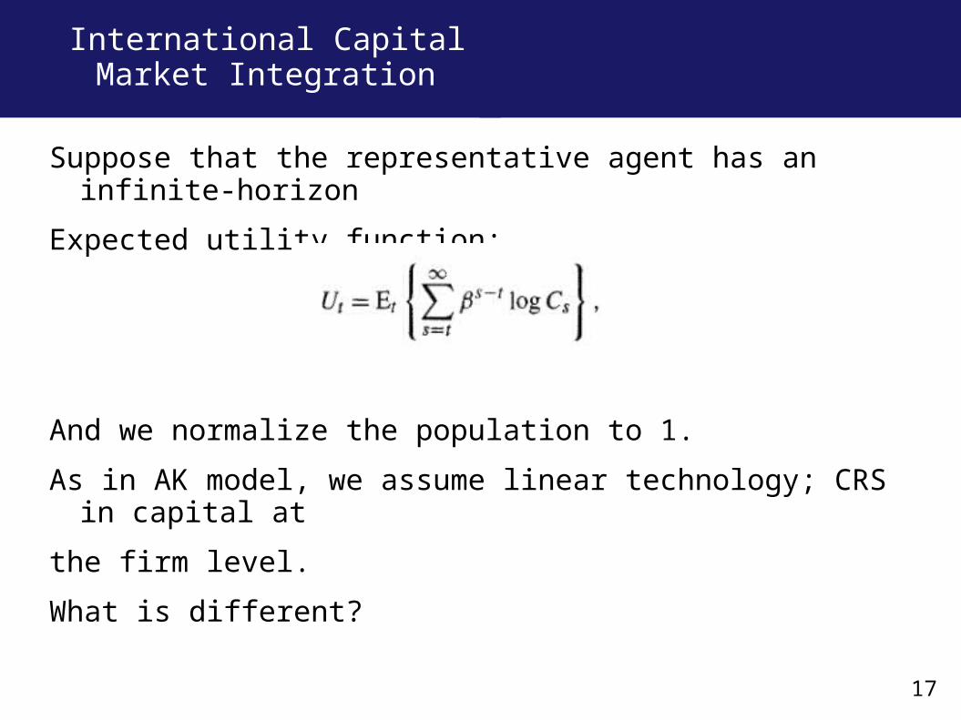
Suppose that the representative agent has an infinite-horizon

Expected utility function:

And we normalize the population to 1.

As in AK model, we assume linear technology; CRS in capital at

the firm level.

What is different?

17


18


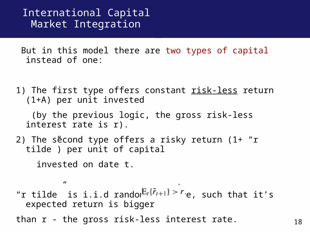
But in this model there are two types of capital instead of one:

1) The first type offers constant risk-less return (1+A) per unit invested

(by the previous logic, the gross risk-less interest rate is r).

2) The second type offers a risky return (1+ “r tilde”) per unit of capital

invested on date t.

“r tilde” is i.i.d random variable, such that it’s expected return is bigger

than r - the gross risk-less interest rate.

18

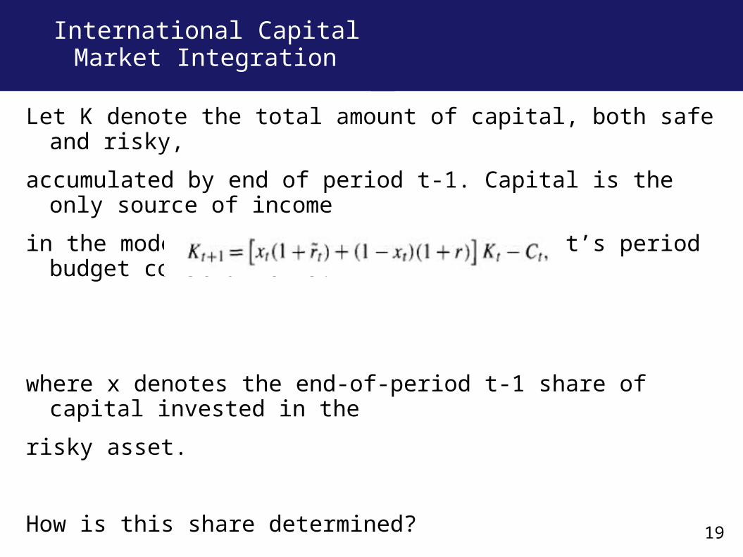
Let K denote the total amount of capital, both safe and risky,

accumulated by end of period t-1. Capital is the only source of income

in the model, so the representative agent’s period budget constraint is:

where x denotes the end-of-period t-1 share of capital invested in the

risky asset.

How is this share determined?

19


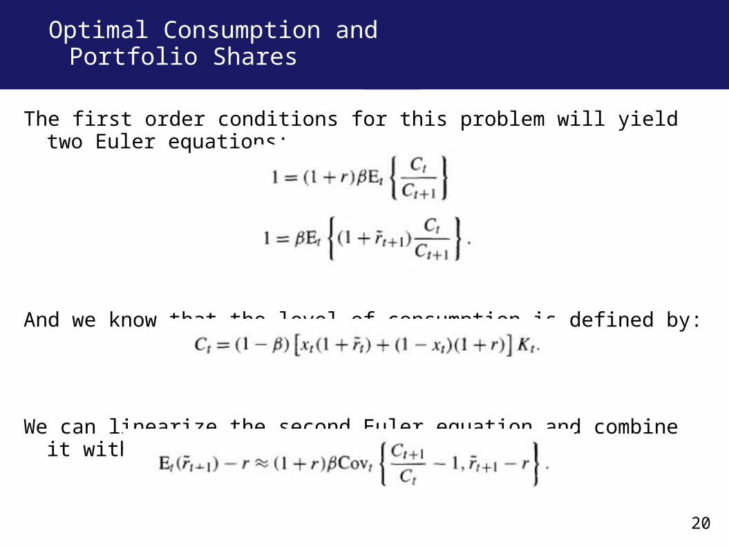
The first order conditions for this problem will yield two Euler equations:

And we know that the level of consumption is defined by:

We can linearize the second Euler equation and combine it with first to yield:

20

Optimal Consumption and Portfolio Shares

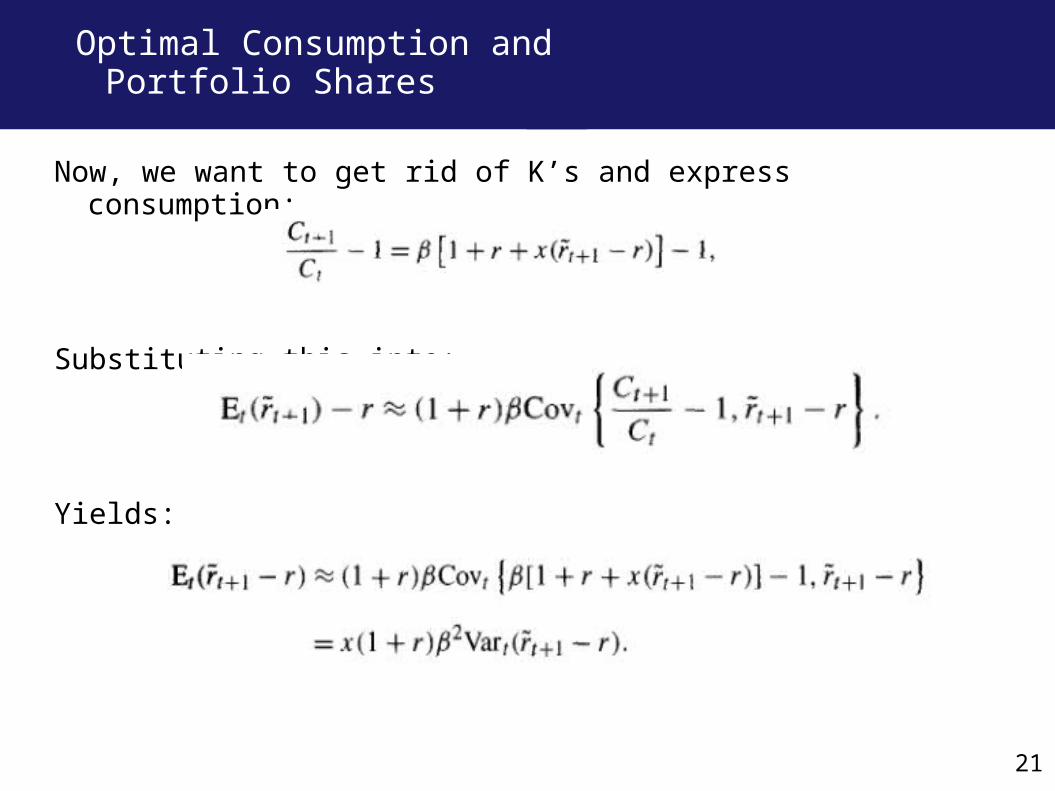
Now, we want to get rid of K’s and express consumption:

Substituting this into:

Yields:

21


22

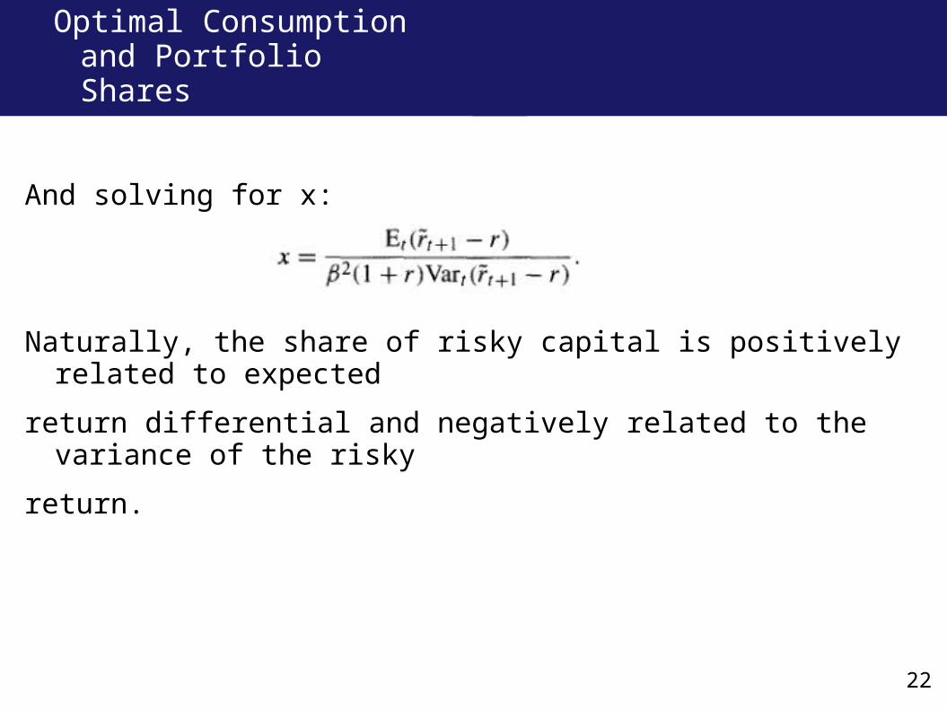
And solving for x:

Naturally, the share of risky capital is positively related to expected

return differential and negatively related to the variance of the risky

return.


22

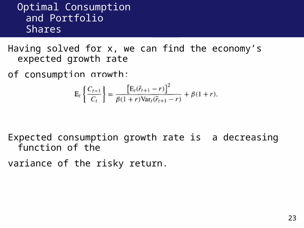
Having solved for x, we can find the economy’s expected growth rate

of consumption growth:

Expected consumption growth rate is a decreasing function of the

variance of the risky return.

23


24

Closed Economy vs. Open Economy

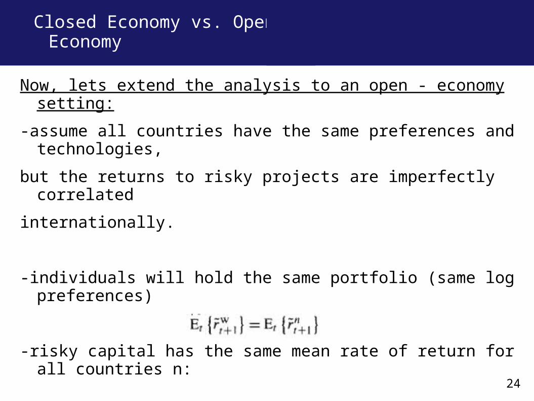
Now, lets extend the analysis to an open - economy setting:

-assume all countries have the same preferences and technologies,

but the returns to risky projects are imperfectly correlated

internationally.

-individuals will hold the same portfolio (same log preferences)

-risky capital has the same mean rate of return for all countries n:

24

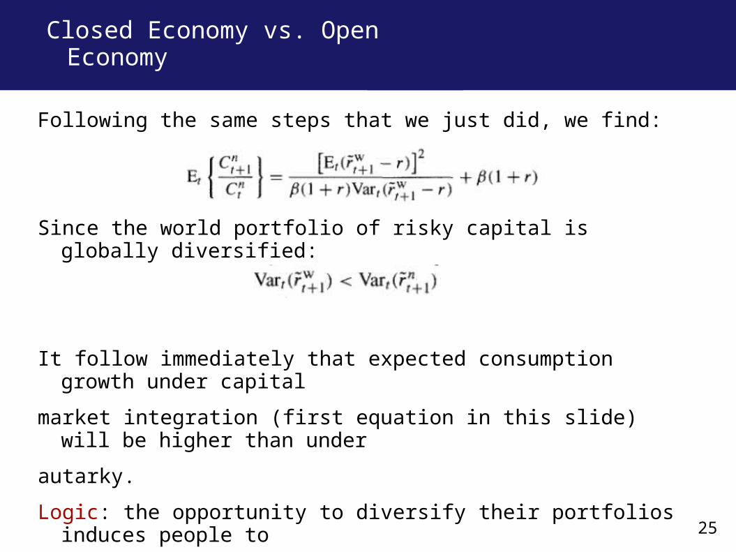
Following the same steps that we just did, we find:

Since the world portfolio of risky capital is globally diversified:

It follow immediately that expected consumption growth under capital

market integration (first equation in this slide) will be higher than under

autarky.

Logic: the opportunity to diversify their portfolios induces people to

allocate a larger share of wealth to risky assets. Hence, expected growth

rises.

25

Closed Economy vs. Open Economy

Comments?

Questions?

26

endogenous growth sophia kazinnik university of houston economics department

Documents