Endogenous Cost Lobbying: Theory and Evidence

John M. de Figueiredo

Duke University and NBER 210 Science Drive

Durham, NC 27708-0360 jdefig@duke.edu

Charles M. Cameron Princeton University

205 Fisher Hall Princeton, NJ 08544

ccameron@princeton.edu

Revised: March 2019

We thank seminar participants at Stanford University, MIT, Harvard University, Princeton University, the University of Chicago, the University of Michigan, UCLA, the University of Palermo, University of North Carolina, George Washington University,

Duke University, and the World Bank, and participants at the Annual Meetings of the Society of Institutional and Organizational Economics, the American Law and Economics Association, the Academy of Management, the American Political Science

Association, and the Midwest Political Science Association. We particularly thank Konstantin Sonin, Tim Groseclose, Keith Krehbiel, Nolan McCarty, Richard Hall, and three referees for detailed and helpful comments. Tom Balmat provided excellent and substantial statistical assistance. Special thanks to Sebastien Thieme who provided us with extremely helpful summaries of

his state-level lobbying data which were employed in revisions to this paper.

Endogenous Cost Lobbying: Theory and Evidence

Abstract

While there has been a substantial growth in the empirical literature on informational lobbying, there has been less

direct testing of the implications of the theoretical models in the area. We provide the first empirical tests of a major

class of models of costly legislative informational lobbying, the Spence-type endogenous cost signaling models. Using

data derived from over 50,000 observations of annual lobbying expenditures in the American states, we find,

substantial support for this class of models’ cross sectional and dynamic predictions. We develop theoretical

extensions to the core model that reflect the variety of observed institutional features of state governments over

multiple periods, and test much more refined and detailed predictions of interest group lobbying controlling for year,

state, and interest group fixed effects. We also test the robustness of these results examining CF-scores and one-sided

interest group lobbying.

Word Count:

Text of Paper (not including this page): 8,742

References: 743

Footnotes: 434

Titles to Figure 1 and Tables 1-10: 73

Total Word Count: 9,992

I. Introduction

One of the main mechanisms that interests groups use to influence policy-making is by finding or producing

information and providing this information to lawmakers through lobbying efforts. Information about the efficacy,

distributional impact, cost, popularity, and legality of programs is extremely valuable to re-election-oriented legislators.

Not surprisingly, then, one finds a “Gucci gulch” of lobbyists outside the committee rooms of Congress and state

legislatures across the county.

Transmitting information to lawmakers – lobbying – is an activity quite distinct, both practically and legally,

from contributing money to political campaigns.1 Nonetheless, informational lobbying requires expenditures by

groups: money to pay lobbyists’ salaries, maintain offices, commission studies, hire experts, and so on. One may gain

at least a rough measure of the extent and importance of informational lobbying by noting that the volume of lobbying

expenditures by special interests at the U.S. federal level is six times that of campaign contributions (de Figueiredo and

Richter 2014).

There have been a number of papers that examine the empirical regularities of informational lobbying.2 This

paper sits as the junction of two currents in the literature. The first current is the analysis of lobbying targeting and

intensity. Here, there are two subcurrents. The first is the micro-political approach. This approach relies on self-

reported survey data, in-depth reviews of public records, and detailed understanding of an issue. These important

studies mostly comprise analyses of one to four issues, up to tens of interest groups, cross-sectional analysis, and

frequently two-sided lobbying (e.g. Austen-Smith and Wright 1994; Honjacki and Kimball 1998, 1999). These papers

have made substantial contributions to understanding targeting, growing a consensus in the literature that both allied

(Caldeira & Wright 1998; Hall & Deardorff 2006; Heberlig 2005; Hojnacki & Kimball 1999; Kollman 1997;

Rotemberg 2003) and marginal legislators on both sides of the issue are targeted for lobbying efforts (Austen-Smith &

Wright 1994, 1996; Bertrand et al 2014; Gawande et al 2012; Holyoke 2003; Kelleher & Yackee 2009). These two

approaches result in a pattern of lobbying where a variety of different legislators are targeted, even by one group, on

1 See de Figueiredo (2002).

2 For an extensive review of the empirical lobbying literature see de Figueiredo and Richter (2014).

the basis of their position in Congress and their position on an issue.3 The studies in the micro-political tradition, while

extremely detailed in who is targeted for lobbying, generally do not describe the intensity of the lobbying effort by the

interest group toward a given targeted legislator over time or over many issues.

The second approach is the macro-political approach. These papers have tended to focus on the intensity of

lobbying. This approach employs large datasets of compulsory lobbyists’ filings and sophisticated statistical analysis.

These important studies comprise hundreds or thousands of interest groups, thousands of issues, and often use both

cross-sectional and time-series analysis to understand the macro-trends in lobbying behavior. Papers in this tradition

show large companies are more likely to lobby than smaller firms (Ansolabehere et al 2002), businesses and trade

associations represent the most intense lobbying groups (de Figueiredo 2004), government attention to an issue attracts

increased lobbying (Leech et al 2005), lobbyists derive their value from both their expertise and their connections

(Bertrand et al 2014), the intensity of city lobbying of state legislatures is determined by city funding and ideological

congruence (Goldstein and You 2017; Payson 2018), and product differentiation amongst firms leads to increases in

lobbying (Kim 2017). The studies in the macro-political tradition, while extremely detailed in their measurement of

the intensity of lobbying, have generally omitted an analysis of targeting.

The second current in political science this paper addresses is the careful testing of formal model implications

that tightly and clearly link theory and testing in a way that can be falsified, to assist the field in supporting and

rejecting broad classes of theoretical models (Clarke & Primo 2012). Along these lines, in both the micro- and macro-

political traditions there is a very small but important literature that directly tests formal models of lobbying (Austen-

Smith & Wright, 1994; Hall & Deardoff 2006; and Kim 2017).4

In this paper, we contribute to both currents in the lobbying literature by attempting to bring an entire class of

game theory signaling models to bear—endogenous cost models—to inform our empirical work and identify how

3 Despite an ongoing debate in some areas, there is consensus in the targeting literature that legislators with agenda-

setting power (Evans 1996) and those on issue-relevant or generally powerful committees (Drope & Hansen 2004) are

likely to be targeted for lobbying.

4 There has been a debate whether theoretical models of lobbying can really be tested with data (see Austen-Smith and

Wright (1996) and Baumgartner and Leech (1996)).

lobbying efforts will respond to different forms of legislative structures and alignment. With respect to the second

current (empirical tests of formal theoretical models), the paper focuses on the most prominent model of informational

lobbying with endogenous costs, the Potters-van Winden-Grossman-Helpman (PWGH) model. To the best of our

knowledge, no empirical paper investigates the predictions of models of Spence-type endogenous cost lobbying

signaling models (Spence 1978).

We start by building the core signaling model and then tailoring it to the institutional structure and alignment

of U.S. states, thus making our model’s prediction more nuanced and reflective of the data. We then employ some of

the most extensive data yet collected on state lobbying expenditures (as distinct from campaign contributions) by

special interest groups. The data were collected from ethics commissions in the American states and include time series

of aggregate lobbying expenditure data from 38 states as well as group-specific annual lobbying expenditures in each

of twelve states, over 50,000 observations. We examine both sets of data. In addition, using the group-specific data, we

construct panel data for groups operating in multiple states. The states involved possess a variety of legislative

institutions, with varying political control and composition. This variation allows us to examine how legislative design

and control affects lobbying expenditures, independent of interest group-specific effects. The expenditures studied here

include approximately $6.7 billion in the aggregate lobbying data and $600 million in the more detailed micro-level

data.5 Thus, the data are well suited for studying expenditures in connection with informational lobbying.

With respect to the first current, our work emanates from the macro-political approach, employing large

datasets across multiple states using panel statistical techniques to predict and describe the overarching trends in the

intensity of lobbying. As we discuss below, the PWGH model predicts that special interest groups increase

informational lobbying expenditures when the legislature is ideologically distant from the interest group. In essence,

5 Detailed expenditure records available in states indicate the bulk of the lobbying expenditures pay the salaries of

lobbyists and their staff, rent for their offices, studies of policies, and fees for expert consultants. None were expended

on campaign advertisements, campaign consultants, campaign literature, get-out-the-vote drives, issue advertising, or

“walking around money.” In fact, it is illegal to report campaign contributions and campaign-type expenditures as

lobbying expenditures. Lobbyists could be corrupt, but such behavior is likely not the mainstream and outside the scope

of this paper.

groups must work harder to persuade a hostile audience. To this extent, we speak to the general effects in the targeting

literature in the micro-political literature. We do not take a stand on whether a group targets “friends” or “enemies” in

their lobbying effort in each of our thousands of group-year observations. We do predict, however, that as the median

voter in the legislature becomes more opposed to an interest group’s position, the interest group will expend more

effort on the people they do choose to target to obtain a favorable policy. We extend the PWGH model to multiple

periods so as to incorporate biennial budgeting. The extended theoretical model makes a series of predictions about

lobbying intensity under different institutional structures and political make-ups. Some of the predictions are

qualitative, indicating the sign of changes. Many of the hypotheses tested are nested, predicting relative levels of

lobbying across institutional structures and relative levels of coefficients. Other hypotheses are rather precise,

predicting a lobbying level that is just not positive for a given institutional structure, but that is, for example, equal to

precisely twice the lobbying level of another institutional structure. The variation in legislative structures and

characteristics across the states enable a rich set of detailed lobbying expenditure hypotheses to be tested. It may be

worth noting that most of these budget predictions are quite distinct from those made by vote buying or campaign

contribution models. In fact, as is widely documented, campaign contributions are closely tied to the electoral cycle

rather than budgeting cycles. Moreover, we know of no theory that would contain all ten of the theoretical predictions,

some with quite precision, of the endogenous cost signaling class of models.

We find strong empirical support for almost all of the model’s predictions. In most cases, the predicted effects

are substantively large, statistically significant, and robust to changes in specifications. To further explore the

robustness of our results, we extend our analysis to consider alternative measurements of interest group ideology and,

perhaps most importantly, issues with one-sided lobbying. The results fare extremely well under both conditions.

Overall, the results provide substantial empirical support for the PWGH class of models of interest group lobbying.

The paper is organized as follows. Section 2 describes the data and initial empirical regularity. Section 3

reviews the PWGH model and extends it to encompass situations when a legislature changes policy only periodically,

as occurs in states with biennial budgeting. Section 4 uses the state data to investigate the PWGH predictions in a series

of empirical tests. Section 5 conducts robustness tests to alternative interest group ideological measurements and one-

sided lobbying. Section 6 discusses the findings and concludes. Appendices A through C contain proofs, theoretical

details, empirical robustness tests, and additional empirical details.

II. The Lobbying Expenditure Data

The Lobbying Disclosure Act of 1995 provided data to scholars on lobbying expenditures at the federal level.

But many state legislatures had already passed similar legislation, creating state ethics commissions that collected data

on lobbying expenditures in the American states. However, little of this data has been collected and analyzed

heretofore.6

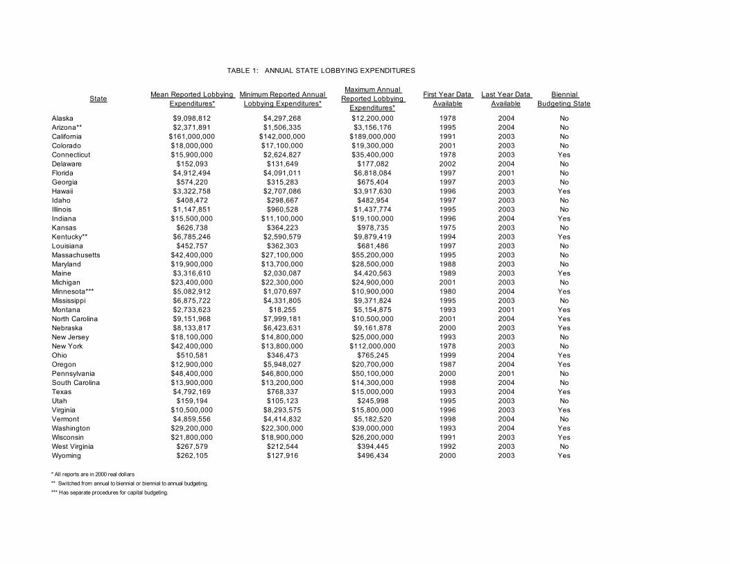
We exploit the state ethics commission data to create three distinct data sets. The first comprises annual

aggregate lobbying expenditures by all interest groups in all states as reported in early 2005, thirty-eight states in all.

Table 1 provides a list of the states, and the time periods for which the data is available and employed in this paper.

This data yields 408 state-year observations.

****INSERT TABLE 1 ABOUT HERE****

The second and more detailed data set consists of annual lobbying expenditures by individual interest groups

in a panel of twelve states: Georgia, Idaho, Indiana, Kentucky, Maryland, Massachusetts, Montana, New Jersey,

Oregon, Virginia, Washington and Wisconsin. These states were chosen on the basis of data quality and availability.

The individual interest group data encompasses more than 50,000 interest-group-state-year observations with lobbying

expenditures. The time periods in the panel average over six years but range from four years to ten years. 7 Each state

averages just over 4,000 observations.

A third data set is derived from this second. It consists of a panel of just over 7,052 interest-_ group-state-year

observations. This sub-sample contains interest groups that are only firms or unions and have lobbied in more than one

budget year in multiple states in the panel.8 There are 600 interest groups which meet these criteria. This sample frame

6 Gray and Lowery (1996) undertook the first substantial effort to examine cross-state level lobbying data with an analysis

of lobbyist registrations.

7 See the Appendix B1 for a discussion of data collection process and comparable datasets.

8 See Appendix B2 for the classification system of interest groups.

is largely driven by the theory, discussed further below. Nevertheless, business and labor interests comprise 42% of

lobbying expenditures recorded.

An obvious issue with the disclosure data is that reporting requirements differ across states. Hence, simple

cross-state differences in lobbying expenditures may largely reflect different legal requirements for reporting

expenditures. Accordingly, in the statistical analyses in the paper, to control for different reporting requirements as well

as other time-invariant unmeasured characteristics, we employ state and interest group fixed effects whenever possible.

To provide an overview of the most striking feature of the data, Figure 1 displays annual lobbying

expenditures in three states with important variation in legislative processes: New York, Wisconsin, and Oregon. New

York has annual regular sessions and annual budgeting, Wisconsin has annual regular sessions but biennial budgeting,

and Oregon has biennial regular sessions and biennial budgeting.

****INSERT FIGURE 1 ABOUT HERE****

The figure suggests a close relationship between lobbying expenditures and the budget cycle (in contrast to

campaign contributions which exhibit a close relationship with the electoral cycle). In particular, Oregon’s and

Wisconsin’s lobbying expenditures increase substantially in budget years, and drop in off-budget years, resulting in a

saw-tooth pattern in expenditures. New York, with annual budgeting, displays no such pattern, however it suggests

there may be non-stationarity in the data (which we address below). Finally, comparing Oregon to Wisconsin, it

appears that regular sessions engender more lobbying intensity than special sessions.

Because previous studies have largely focused on the federal level, where budgeting is annual, the link between

lobbying and budgeting seems to have escaped the notice of analysts using time series data.9 But the pattern is not

difficult to understand. Budgeting forces reconsideration of policy in virtually every arena in which a government is

9 Leech et al (2005) finds a small federal-agency-budget-size effect in a cross-sectional analysis; this data is of only the

U.S. Congress and cannot test budgeting processes. But see also de Figueiredo (2004).

active. Budgeting thus affords a regular opportunity for aggressive claimants to make new or expanded bids on the

public fisc. It also creates a threat – at least potentially – to the rents of virtually every vested interest, as well as the

potential for taxation by the state government and thus rent dissipation for the interest group. In contrast, legislative

action outside the institutionalized budget process requires substantial and sustained investments of time and effort by

legislative entrepreneurs (Arnold 1990). Accordingly, serious change in existing policies, or innovation of new ones, is

rare (Mayhew 1991). Because there is little reason to lobby when the status quo appears inviolable, and considerable

reason to do so when the status quo seems vulnerable, it is no surprise the state data reveals a close link between

lobbying expenditures and budget years in states with biennial budgeting. Moreover, because regular sessions afford

greater scope for legislative action than special sessions, lobbying expenditures predictably are greater in the former

than the latter.

To ensure that this is not merely a spurious correlation, we briefly present a multivariate statistical analysis

confirming the patterns on display in the figure. A battery of augmented Dickey-Fuller and Fisher tests indicates that

some of the longer time series of expenditures, like New York, in this aggregate state-year data are not stationary. The

regressions eliminate the non-stationarity of the data in every state by taking first differences.

We employ a number of independent variables. Table 2 defines each variable and lists its source. Indicator

variables for a budget year and election year for the state legislature are used, as well as variables that measure the

number of days the legislature met in regular session and special session in that year. We characterize the makeup of

the state government as unified Republican, unified Democratic, or divided government. All variables are differenced

within state. In addition, we control for per capita income in the state and use state fixed effects for the 38 states.

****INSERT TABLES 2 AND 3 ABOUT HERE****

In Table 3 we use two different dependent variables: the difference in the log of annual, per capita interest

group lobbying expenditures and the difference in the log of annual interest group lobbying expenditures.

The results across the two models are nearly identical.10 Each 10-day change in the length of the legislative

session results in 6% increase in the lobbying expenditures. The most pronounced effect, however, concerns budget

10 See the Appendix B3 for the methods and approaches for eight alternative specifications considered.

years. Special interests increase their lobbying efforts 23% in years. This result is robust across both specifications

and statistically significant at the 99% level of confidence, controlling for other factors. The patterns shown in Figure 1

seem to be characteristic of broad patterns in the American states.

Having established the importance of the budget cycle to lobbying efforts in this exploratory analysis, we use

this fact and variation in the institutional structures across the states to motivate and explore the validity of theoretical

models of endogenous cost lobbying.

III. Endogenous Cost Lobbying: Theory

Advice-giving by interested or biased parties has spawned a large and complex theoretical literature.

Extensively studied are strategic information transmission by one or more biased advisors using a costless signal, by

one or more advisors using verifiable information, and a single advisor using costly information. The latter class fits

neatly with the state lobby expenditure data, particularly when lobbying is one-sided. Hence, we focus on the class of

lobbying models initiated by Potters and Van Winden (1992) and Austen-Smith (1995) and extended in Grossman and

Helpman (2001: Section 5.2). These models apply the standard technology of costly signaling (“Spence signaling”) to

a political setting; we adapt the models to the specific setting of annual and biennial budgeting. Appendix A1 details

the literature and Appendix A2 assumptions.

A. The Basic Model: Lobbying With Annual Budgeting

In the basic PWGH framework, a legislature (G) has public policy preferences that depend on the state of the

world, a random variable . A special interest group (SIG) has preferences over as well, though in any state of the

world the SIG may prefer higher (or lower) levels of the policy relative to the legislator. In this sense, the SIG is

biased. The SIG, knowing , signals its private information to the decision maker by expending money on lobbying.

In the basic framework, G sets policy, p, de novo, based upon its beliefs about after observing the SIG’s

expenditure.

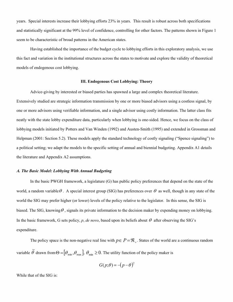
The policy space is the non-negative real line with . States of the world are a continuous random

variable drawn from , . The utility function of the policy maker is

While that of the SIG is:

q q

q

q

+Â=ÎPp

q~ [ ]maxmin ,qq=Q 0min ³q

( )2);( qq --= ppG

where l denotes the monetary expenditure by the SIG.

The degree of SIG bias is parameterized as , which is common knowledge, making the SIG’s ideal point

. Thus, if is positive the SIG wishes a somewhat higher policy than does the policymaker for any state of the

world (positive bias), but if is negative, the SIG wishes a somewhat lower one (negative bias). We associate positive

bias with “liberal” groups and negative bias with “conservative” ones. Bias is defined relative to the legislature. The

sequence of play is: 1) Nature draws using common knowledge distribution ; 2) the SIG (costlessly) learns

and publicly burns money l; 3) the legislature sets policy p.

“Publicly burning money” is not required in a literal sense. The lobbyist could simply invest in more

personnel, elaborate reports or surveys, costly experts, and so on. The key requirements are that the SIG itself chooses

its expenditure level and that the legislator observes the expenditure level. A strategy for the SIG is a function

mapping states of the world into expenditures, . A strategy for the policy maker is a function mapping

expenditures into policy, . An obvious but important point is that, in any equilibrium, the policy maker

will set p to if it knows it.

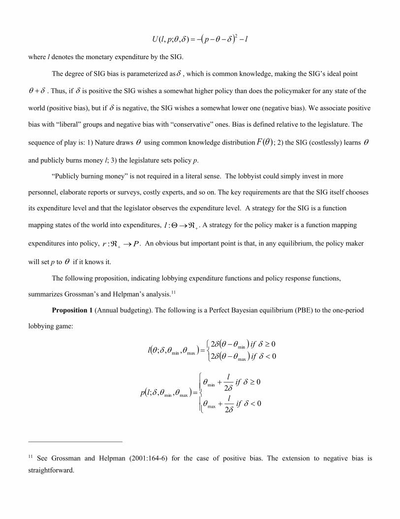
The following proposition, indicating lobbying expenditure functions and policy response functions,

summarizes Grossman’s and Helpman’s analysis.11

Proposition 1 (Annual budgeting). The following is a Perfect Bayesian equilibrium (PBE) to the one-period

lobbying game:

11 See Grossman and Helpman (2001:164-6) for the case of positive bias. The extension to negative bias is straightforward.

( ) lpplU ----= 2),;,( dqdq

d

dq + d

d

q )(qF q

+®Q:l

Pr ®Â+:

q

( ) ( )( )î

íì

<-³-

=0202

,,;max

minmaxmin dqqd

dqqdqqdq

ifif

l

( )ïïî

ïïí

ì

<+

³+=

02

02,,;

max

min

maxmin

dd

q

dd

qqqd

ifl

ifl

lp

Beliefs are determined by Bayes Rule whenever possible.

The intuition behind the result is as follows. The gain to the SIG if G’s belief about is slightly higher is

. To induce truthful revelation, the lobby expenditure function must be such that, at ,

this marginal gain must equal the marginal increase in lobbying expenditure with respect to higher . That is, ,

implying . In addition, lobbying expenditures must be non-negative and equal to zero if for the

case of positive bias, and equal to zero if for the case of negative bias. Importantly, as SIG bias goes to zero,

so does lobbying expenditure: the SIG need not work hard to persuade a legislature whose interests are closely aligned.

But as bias increases, the SIG must work harder to make its case persuasively. The equilibrium is fully separating.

B. Extension: Biennial Budgeting

In some states (e.g., Oregon) the legislature meets only every other year, absent a special session. In these

states, policy is effectively frozen in the off-budget years. In other states (e.g., Wisconsin), the legislature meets

annually but budgeting takes place on a biannual schedule. In these states, modifying budgets in the off-budget year is

not impossible but it is difficult. To analyze lobbying expenditures in states like Oregon and Wisconsin, we extend the

PWGH model to include two periods, a budgeting period and non-budgeting period. Policy is easy to change in the

former; in the latter, it is not.

1. Second Period Equilibrium

Policy making in the budget year establishes a status quo policy, , in place at time 2. The policy maker then

faces a cost of legislating, > 0, to set new policy . The second period utility function for the legislature becomes:

An obvious implication is: if the policy maker knew , it would not legislate unless were sufficiently far from .

If the policy maker alters policy knowing it will set , so the relevant comparison is versus

q

( ) ( )dq ---=¶¶ pUp

2. q=p

q l ¢=d2

dqq 2)( =l minqq =

maxqq =

1p

2k 2p

( )ïî

ïíì

¹---

=--=

if )( action) (no if

),,;(122

222

122

212212

ppkpppp

kppGq

qq

2q 2q 1p

2q 22 q=p ( )221 q-- p

. This implies: do not legislate if . In essence, there is a “hole” in the space and the

policy maker will not legislate if falls in the hole.

We distinguish “high ” states from “low ” ones. In the former, the cost of legislating in the second period

is so high that regardless of the realization of the legislature will not act, i.e., a state where the legislature simply

does not meet in the off-budget years.12 In contrast, in low states there are some realizations of that would lead

the legislature to act, if the value became known. We show in Appendix A3 that high states are defined by

, as this condition assures that the edges of the “hole” extend beyond the

support of . In low states this inequality is reversed, a condition assuring part of the support of lies outside the

“hole.”

In high states lobbying expenditures must be zero in the off-budget years since policy is completely

unresponsive to lobbying, and zero expenditures dominates all other expenditure levels for the SIG. In contrast, in low

states there are levels of that, if known, would lead the policy maker to revise policy. In Appendix A3 we

construct a lobbying expenditure function that induces the SIG to truthfully reveal if it is outside the “hole” and

otherwise indicate that lies in the “hole.” The policy maker sets if lies outside the “hole” and does not

alter policy if it is inside the hole.

Proposition 2 summarizes the second period equilibrium strategies.

Proposition 2 (Off-budget year in states with biennial budgeting). The following comprise second period

strategies in PBE to the two-period lobbying game. 1) High- states: and for all . 2) Low-

states:

12 In practice, all states have provisions where the legislature can be called into special session in the off-budget year. However, for states where the legislature is not already in session, the cost of calling a special session is much higher.

2k- [ ]21212 , kpkp +-Îq 2q

2q

2k 2k

2q

2k 2q

2k

2

11112 },min{},max{21

÷øö

çèæ -+³ ppk qq

2q 2k 2q

2k

2k 2q

2q

2q 22 q=p 2q

2k 12 pp = ( ) 022 =ql 2q 2k

And

Beliefs are determined by Bayes’s Rule where ever possible.

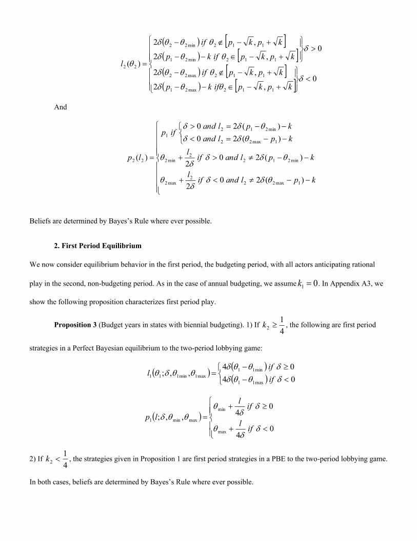
2. First Period Equilibrium

We now consider equilibrium behavior in the first period, the budgeting period, with all actors anticipating rational

play in the second, non-budgeting period. As in the case of annual budgeting, we assume . In Appendix A3, we

show the following proposition characterizes first period play.

Proposition 3 (Budget years in states with biennial budgeting). 1) If , the following are first period

strategies in a Perfect Bayesian equilibrium to the two-period lobbying game:

2) If , the strategies given in Proposition 1 are first period strategies in a PBE to the two-period lobbying game.

In both cases, beliefs are determined by Bayes’s Rule where ever possible.

( ) [ ]( ) [ ]( ) [ ]( ) [ ]ï

ïï

î

ïïï

í

ì

<ïþ

ïýü

+-Î--

+-Ï-

>ïþ

ïýü

+-Î--

+-Ï-

=

0,2

,2

0,2

,2

)(

112max21

112max22

112min21

112min22

22

dqqd

qqqd

dqqd

qqqd

q

kpkpifkp

kpkpif

kpkpifkp

kpkpif

l

ïïïï

î

ïïïï

í

ì

--¹<+

--¹>+

îíì

--=<--=>

=

kplandifl

kplandiflkplandkpland

ifp

lp

)(202

)(202

)(20)(20

)(

1max222

max2

min2122

min2

1max22

min2121

22

qddd

q

qddd

q

qddqdd

01 =k

41

2 ³k

( ) ( )( )î

íì

<-³-

=0404

,,;max11

min11max1min111 dqqd

dqqdqqdq

ifif

l

( )ïïî

ïïí

ì

<+

³+=

04

04,,;

max

min

maxmin1

dd

q

dd

qqqd

ifl

ifl

lp

41

2 <k

In high states, is perfectly revealed but the lobbying expenditure function is twice as steep as in annual

states. In essence, lobby expenditures are shifted into the budgeting year, as the policy lock-in that occurs in the off-

budget year makes the stakes that much higher for the SIG in the budget year. In low states, is again perfectly

revealed and the lobby expenditure function is the same as in the annual states.

C. Empirical Implications

To test the model we utilize the lobbying expenditure functions detailed in Propositions 1-3. However, because

and are unobservable random variables, we take expectations with respect to them to derive expected lobbying

expenditure functions for SIGs over the budget cycle and across different institutional configurations. The four

expected lobbying expenditure functions that result are gathered into Table 4.

INSERT TABLE 4 and TABLE 5 ABOUT HERE

Inspection of the expected lobbying expenditure functions reveals four types of hypotheses, shown in Table 5.

The first concerns the effect of SIG bias on expected lobbying expenditures: regardless of the institutional

configuration, an increase in a SIG’s bias leads (strongly or weakly) to an increase in its lobbying expenditures. We

regard this as the central, critical testable implication of the PWGH framework.

The second group of hypotheses concerns lobbying expenditures in budget years. Ceteris paribus, in budget

years a SIG’s lobbying expenditures should be higher in states with biennial budgeting and high off-year legislation

costs, than in the other two institutional configurations. And, a SIG’s lobbying expenditures in states with annual

budgeting should be indistinguishable from those in biennial states with low off-year legislation costs.

The third group of hypotheses addresses lobbying expenditures in the off-budget years. Ceteris paribus, in off-

budget years a SIG’s lobbying expenditures should be higher in states with annual budgeting, next highest in states

with biennial budgeting and low off-year legislation costs, and lowest in states with biennial budgeting and high off-

year legislation costs. Note that this is the reverse order from that in the second group of hypotheses, a distinctive

feature of the extended PWGH framework.

The fourth group of hypotheses concerns the drop in lobbying expenditures in off-budget years relative to

budget years, in biennial states. Within this group, the following subtle prediction is notable: the ratio of lobbying

2k 1q

2k 1q

1q 2q

expenditures in biennial low-k states between period 1 and 2 should equal the ratio of period 2 lobbying expenditures

between annual states and biennial low-k states.

IV. Data Analysis

In order to test the four main predictions of the PWGH model, we conduct three main sets of analyses. We start by

testing the core prediction in the model, the effect of bias on the amount of endogenous lobbying expenditures. We

then examine the second and third predictions – those concerning inter- or cross-institutional effects by employ two

different estimation methods. Finally, we test the fourth cluster of intra- or within-institutional predictions in high-k

and low-k states over the budget cycle. Appendix B contains a further discussion of data, methods, and results.

A. Core Prediction: Increased Bias Leads to Higher Lobbying Expenditures

We begin by testing the core prediction of the theory: an increase in bias between the legislature and the

interest group leads to higher lobbying expenditures – Hypothesis 1: . Again, this hypothesis does not

predict who will be targeted, but does predict the overall intensity of lobbying conditional on a legislative make-up. In

this subsection, we use 7,052 interest-group-state observations from the twelve-state panel of groups. The groups

analyzed here include all firms and unions operating in multiple states. This sample frame is a natural choice for two

reasons. First, these interest groups frequently have an ideological character (i.e., liberal, conservative) and they are

frequently allied with the major political parties (Democrats for labor, Republicans for firms). Second, by choosing

groups that lobby in multiple states, we can estimate separate interest group fixed effects and state fixed effects. This

sample frame is the third dataset referred to in Section 2.

The dependent variable is the log of lobbying expenditures for group i, in state j, at time t. To measure bias, ,

we create a distance variable which is always positive. This variable measures the ideological distance of the firm

(union) to the legislature. The distance is coded as 0 for a firm if the government (House, Senate, and Governor) is

entirely Republican, and 0 for a union if the government is entirely Democratic. It is coded as 0.5 for both firms and

unions if there is divided government. And it is coded as a 1 for the firm if the government is unified Democratic, and

1 for a union if the government is entirely Republican. In Section V, we utilize more fine-grained measures of firms

( )0³¶¶

dL

d

and unions based on CF-scores. We also include other control variables, such as log of per capita income in the state,

the number days the legislature is in session, and the number of days the legislature is in special session. Group fixed

effects, state fixed effects, and year fixed effects are used, as noted.

Table 6 presents the results. Models 1 through 5 present results with levels. Model 1 uses no fixed effects,

Model 2 adds group fixed effects, Model 3 adds time-varying control variables, Model 4 adds state fixed effects, and

Model 5 includes fixed effects for group, state, and year.

*** INSERT TABLE 6 HERE ***

The coefficient on distance is positive and statistically significant at the 99% level in all specifications. The

inclusion of state fixed effects in Models 4 and 5 causes the size of the coefficient on distance to drop by almost two-

thirds. Substantively, Model 5, with the group, state, and year fixed effects and control variables, estimates there is a

30% increase in lobbying by firms (unions) when the government switches from being unified Republican

(Democratic) to unified Democratic (Republican). Longer regular and special sessions also result in statistically more

lobbying, with each additional 10 legislative days giving rise to 4-5% more lobbying expenditures by special

interests.13

In Models 6 through 10, we replicate the five earlier models using a differences estimator.14 Models 7 through

10 include group, state, and/or year fixed effects as noted, as well. In Model 10, all coefficients are statistically

significant at the 95% or 99% level and all have the same sign as in Model 5. The magnitude of the coefficient on

Distance is somewhat larger than Model 5. It suggests a 73% increase in lobbying by firms (unions) when the

government switches from being unified Republican (Democratic) to unified Democratic (Republican). There is a 5%

increase in lobbying with each additional ten legislative days in the session. That is, a shift in unified government has

almost the same effect as adding 146 session days to the legislative calendar. The effect for special sessions is the

same as the effect of regular sessions in this specification. This result is robust, statistically and substantively

13 For a discussion and alternative estimation approach where legislative session lengths are endogenous to interest group

lobbying, see Appendix B4.

14 This specification addresses concerns of non-stationarity, but certainly the non-stationarity is worth further study.

significant, and consistent with the core prediction of the extended-PWGH model presented in Hypothesis 1, that the

greater the distance between the interest group and the legislature, the more SIG lobbying that occurs.

B. Inter-Institutional Predictions: The Effects of the Budget Cycle on Lobbying

We now employ two different data sets to test the inter- or cross-institutional hypotheses, those shown in

clusters 2 and 3 in Table 5. The first utilizes the individual business-labor data of the previous section and allows us to

estimate the theoretical effects at the micro level. The second utilizes aggregate state level lobbying expenditures from

38 states and allows us to estimate the theoretical effects at the macro level.

In the micro data, we cannot use state fixed effects because of the unvarying state characteristics (i.e. states’

budgetary institutions). Instead, we employ interest group fixed effects, year fixed effects, state random effects, and a

dummy variable, “lax regulations”, which controls for the states’ lobbying expenditures reporting requirements. In the

macro data, we can estimate state fixed effects and then decompose the fixed effects to test the model’s predictions

(following Card and Krueger 1992). We pursue both methods and obtain similar results.

1. Interest Group Level Data

Here we employ the same set of observations as in the previous section. Again, the dependent variable is

logged lobbying expenditures for group i, in state j, at time t. To measure bias, , we utilize the same distance

variable. We retain group fixed effects, year fixed effects, state random effects, and several dummy variables. To

analyze the size of k in the second period, we categorize states into three groups according the standards of the

National Council of State Legislatures (NCSL). The first group comprises states that budget biennially and either do

not meet in the off-year, or have limitations (either legislatively or constitutionally) on the budget bills that can be

considered in the off-year. These are the high-k states with biennial budgeting. The second group comprises states

that budget biennially, meet in the off-year, and have few constitutional or legislative limitations of which types of

bills can be considered in the off-year. These are the low-k states with biennial budgeting. The final group of states

comprises states with annual budgeting; these states are the omitted category in the statistical analysis.15 Finally, as a

15 For a discussion of the categorization by the NCSL, see Appendix B5.

d

partial control for differing expenditure requirements, we include a dummy variable, Lax Regulations, for the states

with the weakest lobbying expenditure disclosure requirements (See Table 2.)

To test the predictions, we must run separate analyses on expenditures in budgeting years and in off-budgeting

years. Thus, we split the sample frame in two: Sample Frame 1 includes budget year data for the sub-sample of

business-labor groups in the 12-state panel, while Sample Frame 2 includes data from the off-budget years for biennial

states and budget years for annual states.

In budget years, the theory predicts groups in low-k states will have similar spending levels as groups in

annual budgeting states (ceteris paribus). However, the theory predicts groups in high-k states will spend at twice this

rate. (See Table 5.) In off-budget years, the theory predicts that group expenditures in low-k states will be lower than

those in annual states. Similarly, group expenditures in high-k states in the off-years are also predicted to be lower than

those in annual states. Additionally, expenditures in high-k states are predicted to be lower than those in low-k states,

in the off-budget years.

*** INSERT TABLE 7 HERE ***

Table 7 presents the results of the estimation. Model 1 uses Sample Frame 1 to test the budget year hypotheses

(Cluster 2 in Table 5); Model 2 uses Sample Frame 2 to test hypotheses about off-budget year expenditures (Cluster 3

in Table 5).

First, note that in both models the coefficient on bias is positive and statistically significant at the 99% level,

again consistent with the core prediction of the theory. A change from a government which is completely aligned with

the SIG’s interest to one which is opposed results in 180% (Model 1) to 134% (Model 2) more lobbying by the SIG,

larger than earlier estimates.

Examining Model 1, the coefficient on Biennial-Low-k is positive but not statistically different from zero,

indicating that lobbying expenditures in budget years in low-k states are not statistically different from lobbying

expenditures in annual states, as predicted. The coefficient on Biennial-High-k is positive and statistically significant at

the 99% level. The point estimate for the coefficient on Biennial-High-k implies that lobbying expenditures in these

states is 82% greater than in annual states. Given the standard error on the coefficient, an F-test fails to reject the

hypothesis that lobbying expenditures in Biennial-High-k states is exactly twice that of annual states. We believe this

is a very stringent prediction and test for a coefficient value. Moreover, an F-test shows that the coefficient on

Biennial-High-k is statistically different and higher than Biennial-Low-k, as predicted. Thus, in this specification, we

find that all predictions in the second hypothesis hold: , , .

Model 2 replicates Model 1 but uses Sample Frame 2 to test the off-budget year hypothesis. The coefficient on

Biennial-Low-k is negative as predicted by the theory, and is statistically significant at the 99% level, lending support

to the Hypothesis 3a (from Table 5). The coefficient on Biennial-High-k is also negative as predicted by the theory,

and statistically significantly different from zero as predicted in Hypothesis 3b. However, an F-test fails to reject the

possibility that off-budget year spending by groups in high-k states is not less than that in low-k states as predicted in

Hypothesis 3c.

Overall, the individual level data show broad support for the theory’s predictions, supporting Hypotheses 2a,

2b, 2c, 3a, and 3b; only Hypothesis 3c does not find support in the individual interest group level data.

2. Aggregate Level Data

We now undertake a two-stage analysis of aggregate expenditure data by state and year (the data used in

Section 2) as a second method for examining these same predictions. In the first stage, we estimate aggregate logged

lobbying expenditures as a function of state fixed effects, plus control variables that vary over time. In the second

stage, we decompose the state fixed effects with cross sectional regressions using non-time varying covariates (Card

and Krueger 1992). The decomposition of the state fixed effects allows tests of the model’s predictions about cross-

institutional effects.

The advantage of the two-stage procedure is its superior ability to control for varying lobby disclosure laws via

the state fixed effects, while still allowing tests of the predictions. However, in order to employ aggregate data, we

must assume that the effect of the second stage variables (low-k, high-k, biennial, total legislatures, etc.) is the same

klowBA LL1

= Akhigh

B LL 21

= klowB

khighB LL

112=

across all interest groups across time.16 Thirty-five state fixed effects are estimated for budget years and thirty-two for

off-budget years.17 These fixed effects become the dependent variables for the second stage regressions.

The results for the first stage regression are found in Appendix B7. The results of the second stage estimation

are shown in Table 8. In addition to the Biennial-High-k, and Biennial-Low-k variables, the second stage regressions

include controls for whether the state has legislative term limits or budget caps, the size of the legislature, the veto

override majority requirements, and an index that describes the degree of professionalization of the legislature. Model

1 examines budget year expenditures while Model 2 examines off-budget years. Both models split the states into high-

k and low-k states.

We first consider the cluster of hypotheses about expenditures in budget years with Model 1. The coefficient

on Biennial-High-k is positive and statistically significant, and the coefficient on Biennial-Low-k is not statistically

different from zero. These results conform to the predictions of the theory in Hypotheses 2a and 2b ( and

). In Table 5, the theory further predicts that expenditures in high-k states will be twice that in annual states

as in Hypothesis 2b ( ). The point estimate of the coefficient on Biennial-High-k indicates that a high-k

state has 70% higher lobbying expenditures relative to annual budget states in the budget years, and an F-test cannot

reject the possibility that at the 95% level of confidence. Finally, the coefficients on Biennial-Low-k and

Biennial-High-k display the same relationship ( , as predicted in Hypothesis 2c) at the 92% level of

confidence, despite only 35 observations.

*** INSERT TABLE 8 HERE ***

We now turn to the hypotheses concerning off-budget year expenditures. Model 2 indicates that both low-k

states and high-k biennial budgeting states have less lobbying in off-budget years than do annual budgeting states, as

predicted by the Hypotheses 3a and 3b. Both low-k and high-k states have 21% less lobbying during these periods.

16 This two-stage estimation procedure cannot be used for the interest group level data in Section IVB1 because interest

group data is available for only 12 states, making the second stage analysis infeasible.

17 We lose some state fixed effects when we difference the data in the first stage.

khighBA LL1

<

klowBA LL1

=

khighBA LL1

2 =

khighBA LL1

2 =

klowB

khighB LL

112=

The data appear to reject the prediction that low-k states have greater lobbying than high-k states in the off-budget

years. (That is, we can reject the prediction in Hypothesis 3c ). Thus, we find support for two of the

model’s three predictions about expenditures in the off-budget years. Overall, the two estimation methods found in

this sub-section, derive qualitatively the same results, finding support for the core hypothesis and five of the six

predictions in the second and third clusters of predictions in both the micro and macro analyses. Only Hypothesis 3c

fails to find support in the analyses.

C. Intra-Institutional Predictions: The Effects of the Budget Cycle on Lobbying

Hypothesis 4a and 4b predict that in biennial budgeting states, expected lobbying expenditures by SIGs is

strictly lower in off-budget years relative to budget years. (That is, and ). As this

observation motivated the construction of the extended model we do not regard these predictions as a strictly valid test

of the model. However, the analyses in Table 9 confirm that the pattern holds in both low-k and high-k biennial

budgeting states. Model 1 demonstrates that lobbying increases 17% in budget years for biennial budgeting low-k

states, and Model 2 demonstrates that it also increases 44% in budget year for biennial budgeting high-k states, relative

to budget years. In addition, as the number of days in a legislative session increases, so does the amount of lobbying

by SIGs. These results are consistent with the first two intra-institutional hypotheses.

*** INSERT TABLE 9 HERE ***

Table 5, however, notes an additional and more subtle prediction about the magnitude of lobby expenditures

over the budget cycle. In particular, the model predicts in Hypothesis 4c : the ratio of off-

budget year expenditures in low-k states to expenditures in annual states, should be the same as the ratio of off-budget

year expenditures in low-k states to budget year expenditures in low-k states. We can use the results in Tables 8 and 9

together to test this prediction from the model. The tables together indicate that while

. An F-test cannot reject the hypothesis that the two ratios are equal to one another, at the 95% level

of confidence. Again, we believe this is a very specific and detailed prediction and test for a ratio of coefficients.

Thus, the data support this more rigorous prediction about expenditures over the budget cycle found in the fourth

hypothesis of the model.

khighB

klowB LL

22>

khighB

khighB LL

21> klow

Bklow

B LL21

>

klowB

klowBA

klowB LLLL

122=

79.2

=Aklow

B LL

86.12=klow

Bklow

B LL

V. Robustness and Extensions

A. Heterogeneity in Interest Groups

One concern that may arise in the previous analysis is that there is measurement error of firms’ and unions’

ideologies. The analysis presented above treats all firms as aligned with Republicans and all unions as aligned with

Democrats, but there could be substantial heterogeneity in these groups’ ideologies.

To address this concern, we employ in this section more fine-grained measures of SIG ideology and distance

where each group has its own unique ideology and thus unique distance measure based on the Bonica (2014) CF-

scores. Here we outline our approach. Appendix C1 details this significant undertaking and presents substantially

more statistical results with this measure.

For all available interest groups, we matched the Bonica CF-scores with our data yielding matches 4,634

observations. We then constructed CF-score measures of the various forms of government. The Distance-CF variable

is the unique distance between each interest group and the state government in power. We then replicate Model 10

from Table 6 in Table 10. Appendix C1 contains detailed replications and discussion of full results.

In Table 10, Model 10CF, the coefficient on Distance-CF is positive and statistically significant at the 99%

level of confidence. The coefficient suggests that a one-point move in CF-Score results in a 28% increase in lobbying.

While the measures of Distance-CF and Distance are not directly comparable, the magnitudes suggest that Distance-

CF results in a similar effect on lobbying as the original Distance measure.

In Table 11, we replicate the models in Table 7, using Distance-CF. Here the results, presented in Model 1CF

and Model 2CF, perform similarly to the main body of the paper. As in Table 7, the coefficient on Distance-CF is both

positive and statistically significant in both models. In Model 1CF, the statistically significant coefficient on Biennial-

High-k implies that lobbying expenditures in these high-k states is 98% greater than annual states, almost exactly the

same as the 100% increase predicted in the theory. The coefficient on Biennial-High-k is statistically different from

Biennial-Low-k, as earlier. In Model 2CF, we explore the off-budget year hypotheses. Appendix C1 discusses the

results in detail. Together, the coefficient values, t-tests, and F-tests provide results consistent with Hypothesis 3a and

3c, but contrary to the predictions of Hypothesis 3b. Overall, the results with Distance-CF mirror the results in the

main analyses congruent with Hypotheses 2a, 2b, 2c, 3a, and 3c.

B. One-Sided Lobbying

A second concern that may arise is that the PWGH theory of lobbying requires only a single lobbying SIG for

the legislature, L, to obtain full information revelation; a second SIG provides no marginal information to L. In our

empirical data, however, there are likely groups lobbying on opposing sides of the issues, known as competitive

lobbying, or in Wilson’s (1980) terminology, interest group lobbying. Interest group lobbying might create random

noise or, at worst, might create biased coefficients.

To address this concern, we examine issues in which we believe there is a predominance of one-sided

lobbying. Because groups on the same side of the issue can coordinate their messaging, the legislature can treat this

information as a single signaler of the information. A number of scholars have identified the pervasiveness of one-

sided lobbying in legislatures. Baumgartner and Leech (2001: 1201), in a sample of 137 issues lobbied at the federal

level find 17% of issues were lobbied by only one group. Baumgartner et al (2009) in a study of federal lobbying on

98 issues find 30% of issues could be considered one-sided (as defined below). Huneeus and Kim (2018), in the most

comprehensive analysis of lobbying to date, analyzed every Lobbying Disclosure Report filed from 1999 to 2018 and

find over 50% of issues are lobbied by only one or two interest groups, most likely on the same side of the issue.

Finally, Thieme (2019b), in his analysis of over 13,000 bills proposed over 13 years in the Wisconsin legislature, finds

that approximately 70% of issues at the state level have one-sided lobbying, as defined below. Thieme (2019a,b) are

the only analyses of this type of which we are aware of state level lobbying, (which is likely quite different from

federal lobbying). This evidence taken together suggests that one-sided lobbying is pervasive in legislatures. In this

subsection our approach is to attempt to identify the issues in our dataset for which there is one-sided lobbying and

then to replicate our analysis on that subset of the data. We do this with two different methods. We outline our

approach and results here and provide more detail and complete results the companion appendices.

1. Thieme (2019a,b)

Our first (and favored) approach is to use Thieme (2019a) data to identify issues in our dataset with one-sided

lobbying. Thieme (2019a) has collected a census of all lobbying on each of the 13,000 bills introduced in the state of

Wisconsin from 2003-2015. Each lobbying SIG identifies its position on each bill (for, against, neutral). We define a

bill as having one-sided lobbying if there are “one or zero groups on one side; everyone else is on the other side,

neutral, or unknown, OR 90% or greater of lobbying groups are on one side.”18 Over 70% of bills introduced into the

Wisconsin legislature are characterized by one-sided lobbying.

Thieme (2019b) categorizes each bill into one of 11 categories. We map our data’s 37 categories into

Thieme’s 11 categories. We impute the Thieme percentages into our data and designate a category as predominated

with one-sided lobbying if it has more than 80% one-sided lobbying. We then replicate our results with this one-sided

lobbying sample frame. We describe the results below. Details of the method and additional results are found in

Appendix C2.

Table 10, Model 10CP presents the replication results from a specification of Table 6, Model 10, with the one-

sided lobbying sample frame. The results are very similar to earlier. A one unit increase in distance is predicted to

have an 82% increase in lobbying. As a further test, Model 10CPCF presents the Thieme one-sided lobbying sample

frame and the Distance-CF measure. Even with both adjustments, the coefficient on Distance-CF is positive and

statistically significant.

In Table 11, we replicate Table 7 using the Thieme’s one-sided lobbying sample frame in Models 1CP and

2CP. The results are strikingly similar to the results in Table 7. Details are in Appendix C2. Suffice it to say here the

coefficients on Distance are both positive and statistically significant, and the coefficient values, statistical

significance, and various F-tests are completely consistent with the main results regarding Hypotheses 2 and 3.

We then replicate this analysis using together the CF-Distance along with the Thieme one-sided lobbying

sample frame, presenting results in Table 11, Model 1CPCF and Model 2 CPCF. The results are similar to the results

found in the previous robustness section of this paper and are consistent with five of the six sub-hypotheses of

Hypotheses 3 and 4.

2. Baumgartner et al (2009)

As an alternative approach, we consider the data found in Baumgartner et al (2009: Table A1). The authors

identify 98 bills over two congresses that were lobbied by interest groups. The authors conducted detailed analysis to

determine the number of groups for, against, and neutral on a given bill. From the position data, we can identify bills

18 We discuss other possible definitions of one-sided lobbying in Appendix C2.

as having one-sided lobbying or interest group lobbying. We mapped the Baumgartner bills into our data’s 37

categories and run a series of weighted OLS regressions that reflect the amount of one-sided lobbying that occurs in

each category. Because 45% of observations are classified in categories with 100% two-sided lobbying, they are

eliminated from our sample frame. We present a much more detailed discussion of this approach and the results in

Appendix C3.

As with the Thieme approach, we have replicated our earlier results in Table 10, Model 10WR. In Model

10WR, the coefficient on Distance is positive, large, and statistically significant at the 99% level of confidence. Its

magnitude suggests a one unit move in distance causes over a doubling in the lobbying expenditures. Overall, the

results of the Baumgartner et al approach are consistent with Hypothesis 1 and the results in the main body of the

paper. In Table 10, Model 10WRCF, we use the more nuanced CF-Distance measures with this weighted regression

approach and the statistically significant results continue to persist. We do not re-estimate Table 7 using our weighted

regression techniques because of limitations in statistical methods for deriving unbiased estimators. A further

discussion is found in Appendix C3.

Overall, the results of both approaches that incorporate only one-sided lobbying yield results that are not only

very similar to the core results in the main body of the paper but are also largely consistent with the signaling theories

of information transmission.

VI. Discussion and Conclusion

In this paper we have examined extensive data on lobbying expenditures in the American states. We used the

data to explore the predictions of the most prominent model of endogenous cost informational lobbying, the Potters-

van Winden-Grossman-Helpman (PWGH) model. Some of the predictions which serve a benchmark for the model’s

testing, such as a group’s lobbying expenditures rising as its preferences move out of alignment with those of the

legislature, are somewhat intuitive, as biased groups must work harder to convince the legislature about policy relevant

conditions. However, the paper extended the basic PWGH model to encompass heterogeneous government power,

heterogeneous interest group ideologies, and time-series variation in budgeting behavior. The extended model makes a

variety of finer-grained predictions about lobbying expenditures across the three institutional designs of annual budgeting,

biennial budgeting with low legislation costs in the off-year (low-k), and biennial budgeting with high legislation costs in

the off-year (high-k). For example, the model predicts that when the likelihood of policy change in the off-years is small

(high-k biennial budgeting), lobbying expenditures shift from non-budget years into budget years such that expenditures

in the budget year of such biennial states should be twice that in annual states. This prediction, and indeed, nine of the ten

predictions generated from the model find support in the empirical analysis. The only prediction that does not find

support is Hypothesis 3c, that low-k states have higher lobbying than high-k states in off-budget years.

Across a variety of alternative specifications using both aggregate and group specific measures, the data strongly

support this prediction. Specifically, we integrate the Bonica (2014) CF-scores into the lobbying data to create unique

distances for each group. In addition, we introduce a series of empirical tests of one-sided lobbying, bringing in datasets

from Thieme (2019a, b) and Baumgartner et al (2009). Although there is substantial descriptive data to suggest that one-

sided lobbying is pervasive, especially at the state level, few studies have focused on this phenomenon specifically, and

never in the context of testing a formal model.

The approach taken in the paper emanates from the macro-political lobbying literature that involves large

datasets, multiple years and issues, and thousands of interest groups. Although we profess to find substantial support for

the PWGH model, parts of these results (such as more lobbying in budget years) could be an artifact of the rising salience

of issues. To the extent that budgeting and salience are highly correlated, it would be difficult to tease these two factors

out in a large-scale study. Likewise, because questions of targeting are beyond the scope of our data, micro-political

studies with in depth analysis of a handful of issues might be a nice complement to the current work in thinking in a more

nuanced way about endogenous cost models of lobbying. Nevertheless, it is unlikely that an alternative theory would find

so many general and specific point predictions.19

In conclusion, it is often claimed that the development of theoretical models in political economy has out-

stripped progress in empirically testing the models. It is perhaps notable, then, when a relatively simple theoretical model

affords demonstrable leverage on extensive data concerning a phenomenon of genuine political significance. Such

appears to the case with the PWGH model.

19 For policy implications of our paper, see Appendices A4 and B6.

REFERENCES Ansolabehere, Stephen, James Snyder, and Micky Tripathi. 2002. “Are PAC Contributions and Lobbying Expenditures

Linked? ” Business and Politics 4(2):131-155. Arnold, R. Douglas. 1990. The Logic of Congressional Action. New Haven: Yale University Press. Austen-Smith, David. 1995. “Campaign Contributions and Access,” American Political Science Review 89(3):566-581. Austen-Smith, David, and John Wright. 1994. “Counteractive Lobbying,” American Journal of Political Science 38:25-

44. Austen-Smith David, and John Wright. 1996. “Theory and evidence for counteractive lobbying,” American Journal of

Political Science 40(2):543-64 Baumgartner FR, Berry JM, Hojancaki M, Kimball DC, Leech BL. 2009. Lobbying and Policy Change: Who Wins,

Who Loses, and Why. Chicago, IL: University of Chicago Press.

Baumgartner, Frank, and Beth Leech. 1996. “Good Theories Deserve Good Data,” American Journal of Political Science 40(1996):565-69

Baumgartner, Frank, and Beth Leech. 2001. “Interest Niches and Policy Bandwagons,” The Journal of Politics 63(2001):1191-1213.

Bertrand M, Bombardini M, Trebbi F. 2014. “Is it whom you know or what you know? An empirical assessment of the lobbying process,” American Economic Review 104(12):3885-3920.

Bonica, Adam. 2014. “Mapping the Ideological Marketplace,” American Journal of Political Science 58(2):367-387. Caldeira Gregory, and Wright, John R. 1998. Lobbying for justice: organized interests Supreme Court nominations, and

United States Senate. American Journal of Political Science 42(2):499-523. Card, David and Alan Krueger. 1992. "Does School Quality Matter? Returns to Education and the Characteristics of

Public Schools in the United States." Journal of Political Economy, 100(1):1-40. Clarke, Kevin, and David Primo. 2012. A Modern Discipline: Political Science and the Logic of Representations. New

York: Cambridge University Press. de Figueiredo, John M. 2002. “Lobbying and Information in Politics,” Business and Politics 4(2):125-129. de Figueiredo, John M. 2004. “The Timing, Intensity, and Composition of Interest Group Lobbying,” NBER Working

Paper #10588, https://www.nber.org/papers/w10588 de Figueiredo, John M. & Brian K. Richter. 2014. “Advancing the Empirical Research in Lobbying,” Annual Review

of Political Science, 17:19.1-19.23. Drope JM, Hansen WL. 2004. Purchasing protection? The effect of political spending on U.S. trade policy. Political

Research Quarterly. 57(1):27-37. Evans D. 1996. Before the roll call: interest group lobbying and public policy outcomes in House committees. Political

Research Quarterly 49(2):287-304. Gawande K, Krishna P, Olarreaga M. 2012. Lobbying competition over trade policy. Inernational Economic Review

53(1):115-32.

Goldstein, Rebecca, and Hye Young You (2017). “Cities as Lobbyists,” American Journal of Political Science

61(4):864-876. Grossman, Gene and Elhanan Helpman. 2001. Special Interest Politics. Cambridge: The MIT Press. Hall RL, Deardorff AV. 2006. Lobbying as legislative subsidy. American Political Science Review 100(1):69-84. Heberlig ES. 2005. Getting to know you and getting your vote: lobbyists’ uncertainty and the contacting of legislators.

Political Research Quarterly 58(3):511-20. Hojnacki M, Kimball DC. 1998. Organized interests and the decision of whom to lobby in Congress. American Political

Science Review 92(4):775-90. Hojnacki M, Kimball DC. 1999. The who and how of organizations’ lobbying strategies in committee. Journal of

Politics. 61(4):999-1024. Holyoke TT. 2003. Choosing battlegrounds: interest group lobbying across multiple venues. Political Research

Quarterly 56(3):325-36. Huneeus, Federico, and In Song Kim. 2018. “The Effects of Firms’ Lobbying on Resource Misallocation,” MIT

Working Paper, http://web.mit.edu/insong/www/pdf/misallocation.pdf Kelleher CA, Yackee SW. 2009. “A political consequence of contracting: organized interests and state agency decision

making. Journal of Public Administration Research Theory 19(3):579-602. Kim, In Song 2017. “Political Cleavages within Industry: Firm-Level Lobbying for Trade Liberalization,” Amerian

Political Science Review 111(1):1-120. Kollman Kenneth. 1997. Inviting friends to lobby: interest groups, ideological bias, and congressional committees.

American Journal of Political Science 41(2):519-44. Leech, Beth, Frank Baumgartner, Timothy LaPira, and Nicholas Semanko. 2005. “Drawing Lobbyists to Washington:

Government Activity and the Demand for Advocacy.” Political Research Quarterly 58(2005):19-30 Mayhew, David. 1991. Divided We Govern. New Haven: Yale University Press. Payson, Julia. 2018. “Cities, Lobbyists, and Representation in Multilevel Government,” NYU Working Paper,

https://drive.google.com/file/d/1I2DD7T5O7syC4LKsg4oqJY0U-qiJlMnF/view Primo, David. 2007. "Stop Us Before We Spend Again: Institutional Constraints on U.S. State Spending," Economics

and Politics 18(3): 269-312. Primo, David, and Jeff Milyo. 2007. “Campaign Finance and Political Efficacy: Evidence from the States,” Election

Law Journal 5(1): 23-39. Potters, Jan and Frans Van Winden. 1992. “Lobbying and Asymmetric Information,” Public Choice 74:269-92. Rotemberg JJ. 2003. “Commercial policy with altruistic voters.” Journal of Political Economy,111(1):174-201 Spence, Michael. 1978. "Job market signaling." Uncertainty in Economics. Academic Press. 281-306. Thieme, Sebastian. 2019a. “Moderation or Strategy? Political Giving by Corporations and Trade Groups,” Journal of

Politics, forthcoming.

Thieme, Sebastian. 2019b. ‘Measuring the Ideology of Private Interests: Evidence of Lobbying Declarations in Three States,” Princeton University Working Paper, https://s18798.pcdn.co/thieme/wp-content/uploads/sites/2501/2018/09/Ideology_and_Extremism_of_Interest_Groups.pdf

Wilson, James Q. 1980. The Politics of Regulation. New York: Basic Books.

State Mean Reported Lobbying Expenditures*

Minimum Reported Annual Lobbying Expenditures*

Maximum Annual Reported Lobbying

Expenditures*

First Year Data Available

Last Year Data Available

Biennial Budgeting State

Alaska $9,098,812 $4,297,268 $12,200,000 1978 2004 NoArizona** $2,371,891 $1,506,335 $3,156,176 1995 2004 NoCalifornia $161,000,000 $142,000,000 $189,000,000 1991 2003 NoColorado $18,000,000 $17,100,000 $19,300,000 2001 2003 NoConnecticut $15,900,000 $2,624,827 $35,400,000 1978 2003 YesDelaware $152,093 $131,649 $177,082 2002 2004 NoFlorida $4,912,494 $4,091,011 $6,818,084 1997 2001 NoGeorgia $574,220 $315,283 $675,404 1997 2003 NoHawaii $3,322,758 $2,707,086 $3,917,630 1996 2003 YesIdaho $408,472 $298,667 $482,954 1997 2003 NoIllinois $1,147,851 $960,528 $1,437,774 1995 2003 NoIndiana $15,500,000 $11,100,000 $19,100,000 1996 2004 YesKansas $626,738 $364,223 $978,735 1975 2003 NoKentucky** $6,785,246 $2,590,579 $9,879,419 1994 2003 YesLouisiana $452,757 $362,303 $681,486 1997 2003 NoMassachusetts $42,400,000 $27,100,000 $55,200,000 1995 2003 NoMaryland $19,900,000 $13,700,000 $28,500,000 1988 2003 NoMaine $3,316,610 $2,030,087 $4,420,563 1989 2003 YesMichigan $23,400,000 $22,300,000 $24,900,000 2001 2003 NoMinnesota*** $5,082,912 $1,070,697 $10,900,000 1980 2004 YesMississippi $6,875,722 $4,331,805 $9,371,824 1995 2003 NoMontana $2,733,623 $18,255 $5,154,875 1993 2001 YesNorth Carolina $9,151,968 $7,999,181 $10,500,000 2001 2004 YesNebraska $8,133,817 $6,423,631 $9,161,878 2000 2003 YesNew Jersey $18,100,000 $14,800,000 $25,000,000 1993 2003 NoNew York $42,400,000 $13,800,000 $112,000,000 1978 2003 NoOhio $510,581 $346,473 $765,245 1999 2004 YesOregon $12,900,000 $5,948,027 $20,700,000 1987 2004 YesPennsylvania $48,400,000 $46,800,000 $50,100,000 2000 2001 NoSouth Carolina $13,900,000 $13,200,000 $14,300,000 1998 2004 NoTexas $4,792,169 $768,337 $15,000,000 1993 2004 YesUtah $159,194 $105,123 $245,998 1995 2003 NoVirginia $10,500,000 $8,293,575 $15,800,000 1996 2003 YesVermont $4,859,556 $4,414,832 $5,182,520 1998 2004 NoWashington $29,200,000 $22,300,000 $39,000,000 1993 2004 YesWisconsin $21,800,000 $18,900,000 $26,200,000 1991 2003 YesWest Virginia $267,579 $212,544 $394,445 1992 2003 NoWyoming $262,105 $127,916 $496,434 2000 2003 Yes

* All reports are in 2000 real dollars** Switched from annual to biennial or biennial to annual budgeting.*** Has separate procedures for capital budgeting.

TABLE 1: ANNUAL STATE LOBBYING EXPENDITURES

Ln(Lobbying Per Capita)State Aggregate Lobbying Expenditures Divided by the Population of the State in a given year, logged (Ethics Commission of Each State where data is available; includes 38 states. Most data is obtain from official disclosures provided.) Population Data from Census and Bureau of Economic Analysis (BEA).

Ln(Lobbying) State Aggregate Lobbying Expenditures in a given year, logged. (Ethics Commission of Each State where data is available; includes 38 states. Most data is obtain from official disclosures provided.)

Interest Group Lobbying Data and Categories

For twelve states, annual lobbying expenditures by registered interest group by year. Categorization of each interest group into each of five categories: corporate, trade association, membership organization, union, and government; for each state for each year. (Ethics Commission of Each State. Most data is obtain from official disclosures provided. N > 50,000)

Budget Year Equal to 1 if the state budget is legally mandated to be created in the year; 0 otherwise. (National Council of State Legislatures--NCSL)

Session Days

The number of legislative days the legislature was in session in that year. For those that reported in calendar days, we divided the number of calendar days by 2.5 to retrieve an approximate number of legislative days. This ratio was determined from a subset of data where both total days and legislative days were reported for the same state-year. Session Dummy is a dummy variable = 1 if the legislature is in regular session and 0 otherwise (Book of the States)

Special Session Days

The number of legislative days the legislature was in session in that year. For those that reported in calendar days, we divided the number of calendar days by 2.5 to retrieve an approximate number of legislative days. This ratio was determined from a subset of data where both total days and legislative days were reported for the same state-year. Special Session Dummy is a dummy variable = 1 if the legislature is in regular session and 0 otherwise (Book of the States)

Election Year Equal to 1 if the legislature holds regularly scheduled election in that year; = 0 otherwise (NCSL)

Republican Government Equal to 1 when the Republican Party holds the governorship, state senate, and state house; = 0 otherwise (Book of the States)

Democratic Government Equal to 1 when the Democratic Party holds the governorship, state senate, and state house; = 0 otherwise (Book of the States)

Ln(Per Capita Income) Log of Per Capita Personal Income of the State in a given year (Bureau of Economic Analysis, Department of Commerce (BEA))

Ln(Population) Log of Population of the State (Census and BEA)

Year Year

Biennial Equal to 1 if a state budgets biennially; = 0 otherwise (NCSL)

Biennial High kEqual to 1 if a state budgets biennially and either does not meet in the off-year, or has limitations on budget bills it can consider in the off-year; = 0 otherwise (NCSL)

Biennial Low kEqual to 1 if a state budgets biennally and meets in the off-year with no restrictions on budget bills that can be introduced; = 0 otherwise (NCSL)

Lax RegulationsEqual to 1 if a state in the 12-state dataset has extremely low reporting requirements, not requiring compensation or other standard disclosure requirements; the states are GA, ID, and MT

Budget Caps Equal to 1 if the state has budget caps; =0 otherwise (Primo, 2007)

Term Limits Equal to 1 if the state has legislative term limits; = 0 otherwise (Primo and Milyo 2007)

Total Number of Legislators The total number of legislators in the state senate and house combined (Book of the States)

Veto Override Requirement The percentage of legislators that must vote for an override of the governor's veto in a given state (Book of the States)

Professionalization IndexA measure of the degree of professionalization of the legislature. This measure is comprised of a rating of the length of the sessions of the legislature, the compensation of legislators, and the amount of staff they have. (Kurtz, NCSL)

Compensation Equal to 1 if the state has a rule regarding the disclosure of lobbyist compensation; = 0 otherwise (Book of the States)

DistanceA measure of the ideological distance of the interest group to the median of the government. It is = 1 if the interest group is a firm (union), and there is Democratic (Republican) unified government. It is = .5 if the interest group is a firm (union), and there is divided government. It is equal to 0 if the interest group is a firm (union) and there is Republican (Democratic) unified government.

TABLE 2: VARIABLES

Model 1 Model 2

Dependent Variable Ln(Lobbying Per Capita)

Ln(Lobbying)

MethodDifferences on

DifferencesDifferences on

Differences

Variable

Budget Year 0.215*** 0.215***(0.06) (0.06)

Session Days 0.006*** 0.006***(0.00) (0.00)

Special Session Days 0.002 0.002(0.00) (0.00)

Election Year -0.039 -0.039(0.04) (0.04)

Republican Government 0.228 0.228(0.13) (0.13)

Democratic Government -0.015 -0.016(0.11) (0.11)

Ln(Per Capita Income) 1.352 1.377(1.20) (1.20)

Constant -0.040 -0.031(0.06) (0.06)

State Fixed Effects Yes Yes

Total R-squared 0.341 0.34F-stat 22.91 22.88

n 351 351

Two-sided t-tests: ** p<.05 *** p<.01

TABLE 3: STATE LOBBYING

Note: Dependent variables and method used are noted. An observation is a state-year.

TABLE 4: EXPECTED LOBBYING EXPENDITURE FUNCTIONS

ANNUAL BUDGETING STATE

BIENNIAL BUDGETING STATE

– LOW

BIENNIAL BUDGETING STATE – HIGH

Period 1

A.

B.

C.

Period 2

D.

E.

F.

TABLE 5: EMPIRICAL PREDICTIONS

CLUSTERS OF PREDICTIONS HYPOTHESES 1. Core hypothesis: Effect of SIG bias on lobbying expenditures 2. Lobbying expenditures in budget years, across institutions a) ; b) ;

c) 3. Lobbying expenditures in off-budget years, across institutions a) ; b) ;

c) 4. Lobbying expenditures over the budget cycle, biennial budgeting states a) ; b)

c) All hypotheses are per SIG, holding bias constant.

2k 2k

( )minmax qqd -=AL ( )min1max11qqd -=klow

BL ( )min1max121

qqd -=khighBL

( )minmax qqd -=AL ( )( )min1max123

22 qqd --= kL klow

B0

2=khigh

BL

0³¶¶dL

klowBA LL1

= Akhigh

B LL 21

=klow

Bkhigh

B LL11

2=klow

BA LL2

> khighBA LL2

>khigh

Bklow

B LL22

>klow

Bklow

B LL21

> khighB

khighB LL

21>

A

klowB

klowB

klowB

LL

LL

2

1

2 =

VariableModel 1 Model 2 Model 3 Model 4 Model 5 Model 6 Model 7 Model 8 Model 9 Model 10

Distance 0.542*** 0.567*** 0.614*** 0.250** 0.267** 0.251** 0.280** 0.282*** 0.317** 0.524***(0.15) (0.08) (0.09) (0.10) (0.11) (0.12) (0.12) (0.12) (0.13) (0.14)

Ln(Population) 0.170*** 2.630 2.060 5.792* 11.581** -11.636*(0.06) (1.55) (1.90) (3.34) (5.23) (6.52)

Ln(Per Capita Income) 1.906*** 0.267 1.576 1.285 0.822 6.784***(0.16) (0.38) (1.28) (0.79) (1.00) (1.47)

Session Days 0.007*** 0.004*** 0.005*** 0.006*** 0.006*** 0.006***(0.00) (0.00) (0.00) (0.00) (0.00) (0.00)

Special Session Days 0.005*** 0.003** 0.004** 0.002* 0.003** 0.004**(0.00) (0.00) (0.00) (0.00) (0.00) (0.00)

Constant 9.071*** 9.058*** -13.551*** -38.980 -42.401 0.052** 0.052*** -0.096** -0.179 -0.339(0.09) (0.05) (1.49) (21.28) (35.65) (0.01) (0.02) (0.04) (0.14) (0.22)

Group Fixed Effects No Yes Yes Yes Yes No Yes Yes Yes Yes

State Fixed Effects No No No Yes Yes No No No Yes Yes

Year Fixed Effects No No No No Yes No No No No Yes

n 7,052 7,052 7,052 7,052 7,052 5,119 5,119 5,119 5,519 5,519

Two-sided t-tests: *p<.10 ** p<.05 *** p<.01

TABLE 6: INTEREST GROUP ANALYSIS FOR MULTI-STATE GROUPS

Levels on Levels Differences

Note: The sample frame is interest groups that engage in multi-state lobbying in 12 states under analysis. The dependent variable is the log of lobbying expenditures by an interest group lobbying in a state-year. Models 1-5 are level on level regression; Models 6-10 are differences on differences regressions. Standard errors, statistical significance, and use of fixed effects are noted. Models 1 and 6 report standard errors clustered on interest group.

Model 1 Model 2

Dependent Variable Ln(Lobbying) Ln(Lobbying)

Method Levels on Levels Levels on Levels

Sample Frame Budget Years for All StatesNon-Budget Years for Biennial States

Budget Years for Annual States

Variable

Distance 1.033*** 0.854***(0.10) (0.12)

Biennial High k 0.599*** -0.320**(0.11) (0.14)

Biennial Low k 0.035 -1.278***(0.14) (0.17)

Session Days 0.002*** 0.002***(0.00) (0.00)

Special Session Days 0.001 0.003(0.00) (0.00)

Ln(Population) -1.014*** -0.333***(0.08) (0.11)

Ln(Per Capita Income) 3.306*** -0.013(0.48) (0.59)

Lax Regulations -3.213*** -4.252***(0.14) (0.17)

Constant -8.380 14.938***(4.30) (4.86)

Group Fixed Effects yes yes

Year Fixed Effects yes yes

State Random Effects yes yes

Wald Statistic 7053.44 6922.74Total R-squared 0.62 0.6278

n 4,966 4,703

Two-sided t-tests: *** p<.01, **p<.05

TABLE 7: INTER-INSTITUTIONAL EFFECTS USING INTEREST GROUP DATA

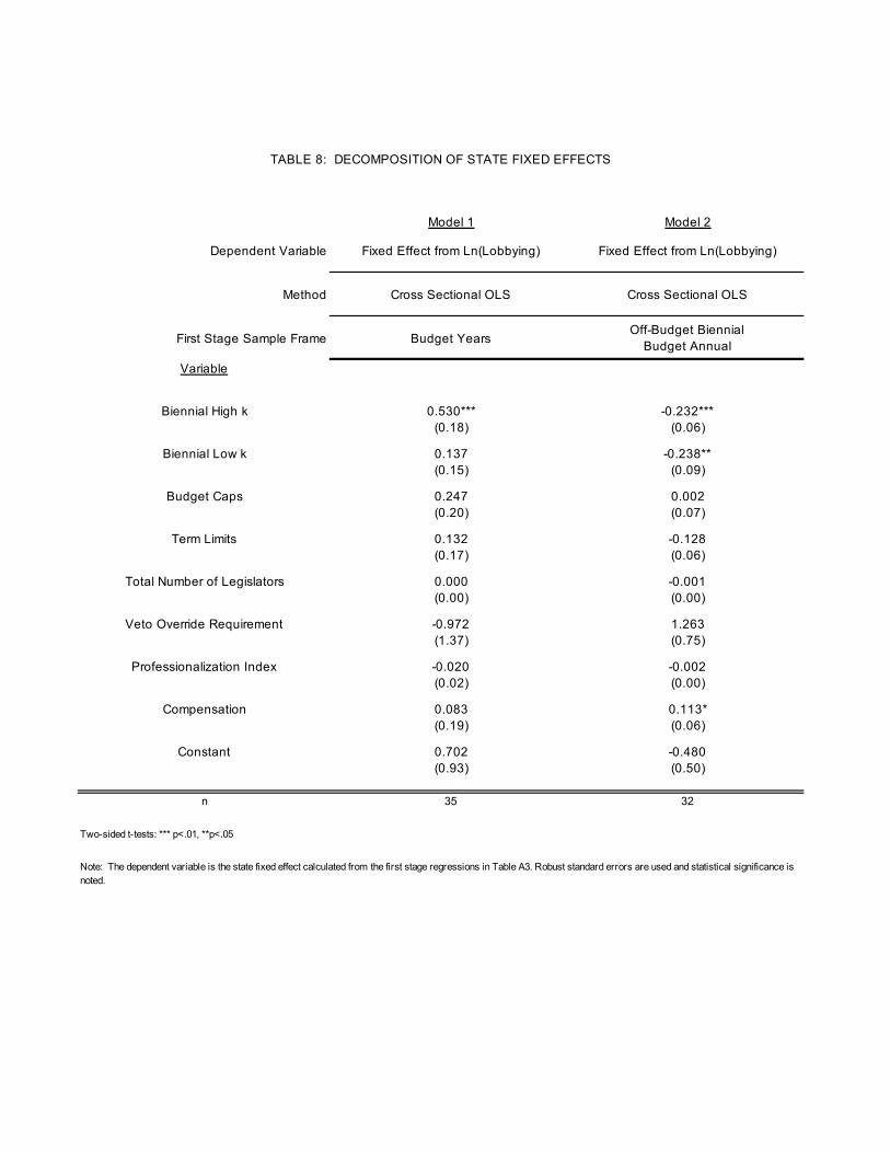
Model 1 Model 2

Dependent Variable Fixed Effect from Ln(Lobbying) Fixed Effect from Ln(Lobbying)

Method Cross Sectional OLS Cross Sectional OLS

First Stage Sample Frame Budget YearsOff-Budget Biennial

Budget Annual

Variable

Biennial High k 0.530*** -0.232***(0.18) (0.06)

Biennial Low k 0.137 -0.238**(0.15) (0.09)

Budget Caps 0.247 0.002(0.20) (0.07)

Term Limits 0.132 -0.128(0.17) (0.06)

Total Number of Legislators 0.000 -0.001(0.00) (0.00)

Veto Override Requirement -0.972 1.263(1.37) (0.75)

Professionalization Index -0.020 -0.002(0.02) (0.00)

Compensation 0.083 0.113*(0.19) (0.06)

Constant 0.702 -0.480(0.93) (0.50)

n 35 32

Two-sided t-tests: *** p<.01, **p<.05

TABLE 8: DECOMPOSITION OF STATE FIXED EFFECTS

Note: The dependent variable is the state fixed effect calculated from the first stage regressions in Table A3. Robust standard errors are used and statistical significance is noted.

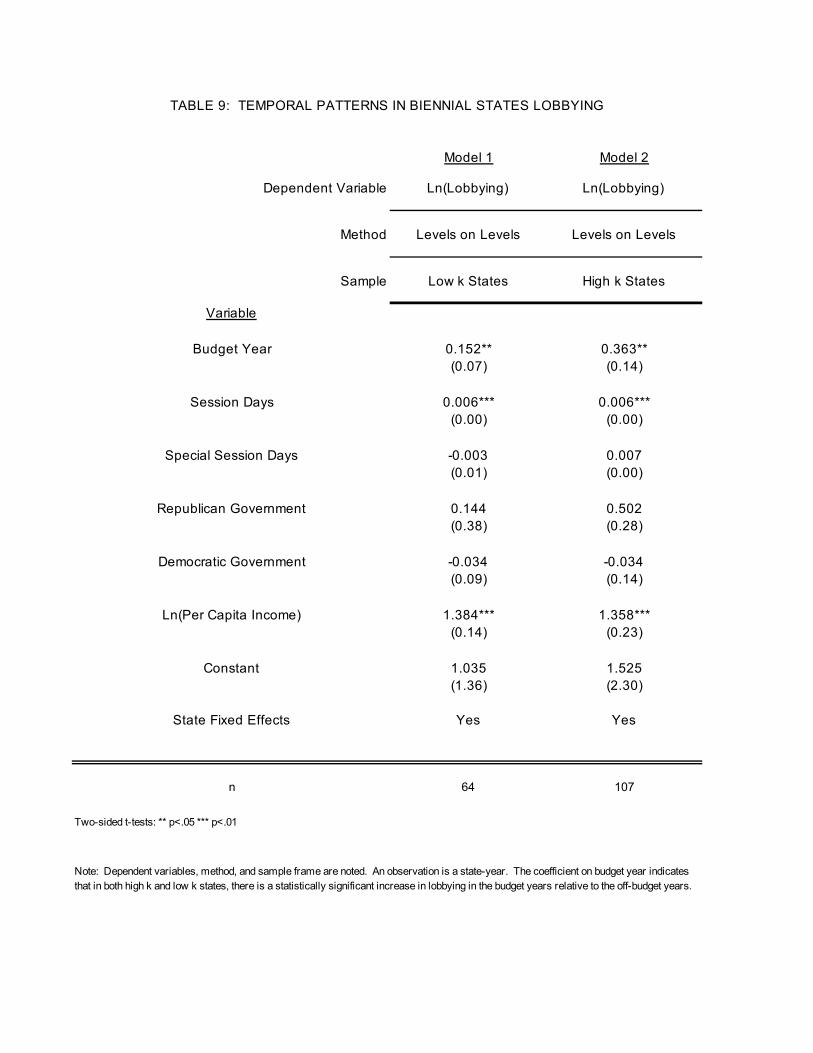
Model 1 Model 2

Dependent Variable Ln(Lobbying) Ln(Lobbying)

Method Levels on Levels Levels on Levels

Sample Low k States High k States

Variable

Budget Year 0.152** 0.363**(0.07) (0.14)

Session Days 0.006*** 0.006***(0.00) (0.00)

Special Session Days -0.003 0.007(0.01) (0.00)

Republican Government 0.144 0.502(0.38) (0.28)

Democratic Government -0.034 -0.034(0.09) (0.14)

Ln(Per Capita Income) 1.384*** 1.358***(0.14) (0.23)

Constant 1.035 1.525(1.36) (2.30)

State Fixed Effects Yes Yes

n 64 107

Two-sided t-tests: ** p<.05 *** p<.01

TABLE 9: TEMPORAL PATTERNS IN BIENNIAL STATES LOBBYING

Note: Dependent variables, method, and sample frame are noted. An observation is a state-year. The coefficient on budget year indicates that in both high k and low k states, there is a statistically significant increase in lobbying in the budget years relative to the off-budget years.

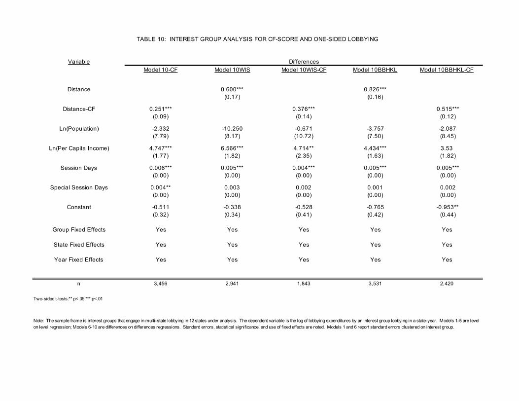
VariableModel 10-CF Model 10WIS Model 10WIS-CF Model 10BBHKL Model 10BBHKL-CF

Distance 0.600*** 0.826***(0.17) (0.16)

Distance-CF 0.251*** 0.376*** 0.515***(0.09) (0.14) (0.12)

Ln(Population) -2.332 -10.250 -0.671 -3.757 -2.087(7.79) (8.17) (10.72) (7.50) (8.45)

Ln(Per Capita Income) 4.747*** 6.566*** 4.714** 4.434*** 3.53(1.77) (1.82) (2.35) (1.63) (1.82)

Session Days 0.006*** 0.005*** 0.004*** 0.005*** 0.005***(0.00) (0.00) (0.00) (0.00) (0.00)

Special Session Days 0.004** 0.003 0.002 0.001 0.002(0.00) (0.00) (0.00) (0.00) (0.00)

Constant -0.511 -0.338 -0.528 -0.765 -0.953**(0.32) (0.34) (0.41) (0.42) (0.44)

Group Fixed Effects Yes Yes Yes Yes Yes

State Fixed Effects Yes Yes Yes Yes Yes

Year Fixed Effects Yes Yes Yes Yes Yes

n 3,456 2,941 1,843 3,531 2,420

Differences

TABLE 10: INTEREST GROUP ANALYSIS FOR CF-SCORE AND ONE-SIDED LOBBYING

Two-sided t-tests:** p<.05 *** p<.01

Note: The sample frame is interest groups that engage in multi-state lobbying in 12 states under analysis. The dependent variable is the log of lobbying expenditures by an interest group lobbying in a state-year. Models 1-5 are level on level regression; Models 6-10 are differences on differences regressions. Standard errors, statistical significance, and use of fixed effects are noted. Models 1 and 6 report standard errors clustered on interest group.

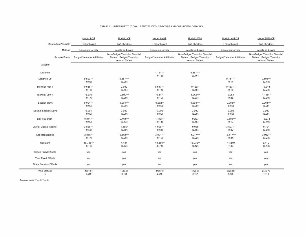
Model 1-CF Model 2-CF Model 1-WIS Model 2-WIS Model 1WIS-CF Model 2WIS-CF

Dependent Variable Ln(Lobbying) Ln(Lobbying) Ln(Lobbying) Ln(Lobbying) Ln(Lobbying) Ln(Lobbying)

Method Levels on Levels Levels on Levels Levels on Levels Levels on Levels Levels on Levels Levels on Levels

Sample Frame Budget Years for All StatesNon-Budget Years for Biennial

States, Budget Years for Annual States

Budget Years for All StatesNon-Budget Years for Biennial

States, Budget Years for Annual States

Budget Years for All StatesNon-Budget Years for Biennial

States, Budget Years for Annual States

Variable

Distance 1.121*** 0.861***(0.13) (0.16)

Distance-CF 0.593*** 0.587*** 0.761*** 0.696***(0.06) (0.08) (0.11) (0.13)

Biennial High k 0.688*** 0.002 0.617*** -0.452** 0.483*** -0.213(0.13) (0.16) (0.14) (0.18) (0.18) (0.23)

Biennial Low k 0.279 -0.890*** 0.117 -1.363*** 0.054 -1.169***(0.17) (0.20) (0.19) (0.23) (0.25) (0.29)

Session Days 0.004*** 0.004*** 0.002** 0.003*** 0.003** 0.004***(0.00) (0.00) (0.00) (0.00) (0.00) (0.00)

Special Session Days 0.001 0.003 -0.000 0.002 0.002 0.000(0.00) (0.00) (0.00) (0.00) (0.00) (0.00)

Ln(Population) -0.914*** -0.461*** -1.112*** -0.227 -0.895*** -0.273(0.09) (0.13) (0.11) (0.15) (0.13) (0.19)

Ln(Per Capita Income) 3.866*** 1.195* 4.005*** -0.065 3.697*** 0.721(0.58) (0.70) (0.64) (0.78) (0.82) (0.99)

Lax Regulations -2.968*** -3.861*** -3.091*** -4.277*** -3.117*** -3.963***(0.17) (0.20) (0.19) (0.22) (0.24) (0.28)

Constant -15.788*** 4.181 -13.850** 13.935** -14.249 6.110(5.18) (5.83) (5.74) (6.42) (7.33) (8.18)

Group Fixed Effects yes yes yes yes yes yes

Year Fixed Effects yes yes yes yes yes yes

State Random Effects yes yes yes yes yes yes

Wald Statistic 4807.04 4500.38 4100.40 4250.93 2525.08 2516.75n 3,259 3,131 2,910 2,747 1,795 1,710

Two-sided t-tests: *** p<.01, **p<.05

TABLE 11: INTER-INSTITUTIONAL EFFECTS WITH CF-SCORE AND ONE-SIDED LOBBYING