Endogenous Comparative Advantage∗

Andrea Moro,

Vanderbilt University, Nashville TN 37235 (USA), andrea@andreamoro.net

Peter Norman,

University of North Carolina at Chapel Hill, Chapel Hill NC 27599 (USA), normanp@email.unc.edu

March 2, 2018

Abstract

We develop a model of trade between identical countries. Workers endogenously acquire skills

that are imperfectly observed by firms, who therefore use aggregate country investment as the prior

when evaluating workers. This creates an informational externality interacting with general equilib-

rium effects on each country’s skill premium. Asymmetric equilibria with comparative advantages

exist even when there is a unique equilibrium under autarky. Symmetric, no-trade equilibria may

be unstable under free trade. Welfare effects are ambiguous: trade may be Pareto improving even

if it leads to an equilibrium with rich and poor countries, with no special advantage to country size.

Keywords: Trade, Specialization, Human Capital, Reputation.

JEL Classification Number: D62, D82, F11, O12

∗Forthcoming: Scandinavian Journal of Economics, DOI: 10.1111/sjoe.12291. It is nearly impossible tothank everybody that contributed comments and suggestions. We thank them all, especially the anonymousassociate editor and two referees. Support from NSF Grants #SES-0003520, #SES-0110131 (Moro), #SES-0001717 and #SES-0096585 (Norman) is gratefully acknowledged.

1

I Introduction

In this paper we develop a stylized model of international trade in which a country can

establish a reputation for having a high quality labor force, providing new insights to the

understanding of the causes of trade, specialization, and inequality across countries.

A reputation for high or low quality of the labor force may arise when employers do not

perfectly observe workers’ competencies and skills. Workers acquire human capital not only

through education and work experience, but also with personal effort and investments that

are not as easily observable. We focus on this informational asymmetry, showing that it may

generate self-fulfilling reputational differences across countries.

Research has shown that informational asymmetries of this kind are empirically relevant.

Farber and Gibbons (1996) and Altonji and Pierret (2001) first showed that employers’ learn-

ing is significant, supporting the assumption that employers initially observe workers’ skills

with noise.1 Recent literature confirms these results2 suggesting a significant scope for the

mechanism proposed in this paper to play a role in determining workers’ wage distribution,

incentives to acquire skills, and sorting across industries.

Based on this evidence, one cannot dismiss the possibility that labor market informa-

tional asymmetries may play a role in explaining, at least in part, trade and specialization

across countries. In this paper, we demonstrate that they are sufficient to generate self-

fulfilling cross-country differences in reputation that imply human capital differences, trade,

and specialization between otherwise identical countries. There is arguably an incomplete

1In most of the literature, the identification of the main effect exploits panel data where workers areobserved over time. If employers imperfectly observe workers’ skills, but learn over time through the obser-vation of productivity signals, then as tenure increases wages should become more correlated with measuresof productivity available to the researcher (typically, workers’ scores in aptitude tests).

2In particular, Lange (2007) measured the “speed” of employer learning finding that, according to thebest estimates, it takes three years for an employer to reduce her expectation error to 50 percent of its initialvalue, and 26 years to reduce it to less than 10 percent of its initial value. Note that median employeetenure is currently just above 4 years, (January 2016, see the U.S. Bureau of Labor Statistics news release“Employee Tenure”, https://www.bls.gov/news.release/tenure.toc.htm, last accessed: February 9, 2018).See also Schonberg (2007), Pinkston (2009), and Kahn and Lange (2014) using U.S. data, and Lesner (2017)with Danish data. Cornwell et al. (2017) use Brazilian data to show that employer variation in workers’perceived race significantly affects wages.

2

understanding of the patterns of trade and specialization observed in the real world, which

suggests that exploring alternative models could provide new insights.3

In our model, technology has constant returns to scale, a country is defined as a la-

bor market, and international trade is frictionless. Countries are symmetric in every respect,

therefore the model always admits symmetric equilibria that replicate autarky, without gain-

ful trade. The only aspect of the model that is non-standard is workers’ skill acquisition.

We investigate the conditions that generate equilibria with asymmetric country reputations

for skill investments and show the properties of such equilibria.

Workers can acquire skills at a cost that varies across workers. There are two sectors de-

manding labor, a “high tech” sector and a “low tech” sector, and skills increase productivity

only in the high tech sector. Incentives to acquire skills are affected by an informational

asymmetry: workers’ skills are only observed by employers with noise, through a signal of

productivity that may be thought of as aggregating information provided by the worker’s

curriculum, interviews, and observation in the workplace. A worker without skills, which we

henceforth call an unqualified worker, may send a good signal, but this is less likely than a

qualified worker (a worker with skills) sending a good signal.

Before observing the noisy signal, the prior probability of investment is determined in

each country by aggregate investment rates summarized by the proportion of qualified work-

ers. The probability of investment of each worker is then computed using her signal, but is

also affected by the prior. Hence, the actual proportion of qualified workers, together with

endogenous relative prices, determines incentives to invest. There is no point in investing in

skills if there are very few qualified workers in the country because firms interpret a good

signal as most likely being noise and the good signal raises the wage very little. Symmetri-

cally, if almost all workers invest, firms ignore bad signals as “bad luck,”and again there is

no point in investing since all workers get high wages regardless of the signal. Incentives to

invest are at the highest at some intermediate level of aggregate investment because this is

3A full empirical investigation of the model implications, which would require accounting for (and sepa-rately identifying) other relevant factors, is outside the scope of this paper.

3

when firms pay most attention to the noisy signals.

Hence, starting from a relatively low level of investments, the value to acquire human

capital increases if the proportion of skilled workers in the economy increases as the signal

to noise ratio decreases. Working against this there are relative price effects that make

the high-tech good less valuable when its supply increases, but these effects are smaller

when countries trade than in autarky. Additionally, when skills increase in one country, the

incentives to acquire skills in the other country are unambiguously reduced because of the

price effects. Hence, an asymmetric allocation of human capital and goods production may

arise even if countries are fundamentally identical. As far as we know, this is an explanation

of trade and specialization that is novel in the international trade literature. What is crucial

for this result is that the reputation for having a qualified labor force is like a public good,

operating within a country regardless of its size.

While our mechanism is novel, there are some similarities with models of agglomeration.

Scale economies and network effects can also create asymmetries between countries. How-

ever, these models usually assume some exogenous differences that are being accentuated in

equilibrium. Moreover, in these models it is typically an advantage to have a large domestic

market, whereas in our model there is no systematic effect favoring large countries. It is

not the number, but the proportion of qualified workers that is critical in generating the

reputational externality because employers, when assessing workers, use the proportion of

qualified worker as their prior for human capital investment. A worker is more likely to be

qualified the higher her country’s proportion of qualified workers.

We highlight this irrelevance of country size by showing that large economies have no

systematic advantage. In many parameterizations where country sizes are allowed to differ,

there is an equilibrium where the large country is the richer as well as an equilibrium in

which the small country is the richer. Which of these equilibria leads to more inequality or

higher welfare is also a matter of parameter choices.

Asymmetric equilibria arise under free trade, but as already noted, there is always at

4

least one symmetric equilibrium with no gainful trade that replicates the autarky allocation.

However, several properties of our model suggest that coordinating on an asymmetric equi-

librium may be plausible.4 First, this is not a model in which some countries are trapped in

a coordination failure and others are not. Incentives in one country depend on investments

in the other and relative price effects are crucial. Asymmetric equilibria may therefore occur

even if the autarky equilibrium is unique. Moreover, the stability conditions under autarky

differ from the stability conditions under free trade. Opening up international trade may

destabilize the unique and stable autarky equilibrium, so cross country income differences

may be an inevitable aspect of free trade even if there are no exogenous differences that

“explain” which country becomes richer.

In any asymmetric equilibrium, a country with more human capital is richer and better

off than the other country. However, this does not necessarily imply that the poor country

is worse off under trade than autarky. Welfare in the poor country can go either way, but

we emphasize the less intuitive possibility by showing an example where an asymmetric

equilibrium Pareto dominates the autarky equilibrium. The intuition is that an increase in

the skill level abroad may drive down the relative price of the high-tech good so much that

exchanging the low-tech good for the high-tech good generates higher welfare in the poor

country compared to domestic production.

Our results are robust to introducing exogenous productivity differences. If one country

has a “fundamental” comparative advantage in the high-tech industry, it may still specialize

as a low-tech industry as a result of the mechanism in our model, provided that the exogenous

differences are not too large.

The next section discusses the contribution of this paper relative to existing literature.

Section III introduces the model, defines the equilibrium, and shows that it can be character-

ized as a planner’s problem, simplifying the analysis that follows. Section IV characterizes

the equilibria under autarky. The main result, the existence of equilibria with trade and spe-

4Matsuyama (2002) argues that multiplicity by itself does not offer a compelling reason for observedasymmetries.

5

cialization, is presented in Section V. Section VI discusses the stability and welfare properties

of equilibria with trade, and the irrelevance of size. Section VII concludes discussing the ro-

bustness of the results to extending the model to multiple countries, to including physical

capital, and migration.

II Related literature

Our main contribution to the literature is to suggest a novel source of trade and comparative

advantage between identical countries. There are several papers in the literature that include

some of the crucial elements of our model, imperfectly observed human capital accumulation,

but in those models either some exogenous differences are posited, or equilibrium multiplicity

in a baseline autarky model is the driving source of specialization.

Our model relates to a literature on trade and endogenous skill formation initiated by

Findlay and Kierzkowski (1983), who develop a general equilibrium model where the driver

of trade is endogenous human capital acquisition as in our model. Countries specialize

because of exogenous differences in the availability of inputs needed to acquire human capital,

generating what we refer to as price effects. In our setup instead, countries are identical also

in the cost of acquiring human capital.5

Among the papers presenting models with asymmetric information, Grossman and Maggi

(2000) and Grossman (2004) have elements that are similar to our setup: a Hecksher-Ohlin

model with imperfectly observable skills. They focus on comparative statics with respect

to changes in the skill distribution. For their purposes it is sufficient to consider how trade

is affected by exogenous differences in the talent distribution across countries, ignoring the

incentives to acquire skills that are central in our model.6

5The focus of this literature is mainly in showing how even if factor price equalization holds (for themarginal worker), trade induces different incentives to acquire human capital across countries. For recentextensions see also Ranjan (2001), Falvey et al. (2010), Auer (2015), Unel (2015), Blanchard and Willmann(2016), and Danziger (2017). In some cases, the exogenous country differences are assumed by analyzing theeffects of trade on a small open economy that takes the world price as given, as in Cartiglia (1997), Bougheaset al. (2011), Bonfatti and Ghatak (2013), or Harris and Robertson (2013).

6Several papers study the effects of informational asymmetries on trade, without focusing on how trade

6

Costinot (2009), like us, seeks to formulate a more fundamental theory of comparative

advantage. The technology is also based on the idea that human capital is more important

for some firms than for others. The main difference is that the model ultimately derives

country differences from exogenous differences in institutional quality and human capital.

Chisik (2003) derives trade in a model where products may acquire, in equilibrium,

different reputation for quality. Self-fulfilling reputation determines the average quality

of a country exports, and comparative advantages arise endogenously because countries

coordinate on selecting different equilibria.7 Similarly, in Chatterjee (2017) comparative

advantages emerge endogenously as a Nash equilibrium of a game in which countries choose

policies that affect sector-specific productivities or relative factor endowments. In these

papers equilibrium multiplicity is needed to generate the comparative advantage. In our

model instead, trade may arise even when there is a unique autarky equilibrium.

While our underlying assumptions are very different, our model shares many features

with trade models with increasing returns (Ethier (1982), Krugman (1980)), their versions

usually referred to as “agglomeration models” (Krugman and Venables (1995), Puga and

Venables (1999)), and the “symmetry-breaking” literature (see Matsuyama (1996, 2004)).

Agglomeration models can sustain a concentration of (high-income) manufacturing because

production costs decrease with the size of the industry. Manufactured goods are inputs in

the production of other goods, implying that being close to other producers saves on trans-

portation costs. This creates incentives to concentrate production. When production costs

arises in equilibrium. Vogel (2007), studies the effect of institutional quality on reducing workers’ moralhazard. Davidson and Sly (2014), study how trade affects one country’s human capital accumulations wheneducation has a signaling role. Park (2011) analyzes trade agreements under imperfect public monitoring,Zhang (2012) consider effects of asymmetric information when exporters are credit constrained, and Creaneand Jeitschko (2016) show that weak institutions may result in welfare-reducing trade in an adverse selec-tion model. Razin and Sadka (2003) use an informational asymmetry to model the role of foreign directinvestments, Casella and Rauch (2002) derive a role for minority groups in international trade using aninformational friction, and McCalman (2002) considers the impact of asymmetric information in bargainingabout trade agreements. Eicher (1999) considers a model that is significantly richer than ours in many ways,but the informational asymmetry is modeled in reduced form.

7Other models based on trust and endogenous quality reputation are Araujo and Ornelas (2007), Araujoet al. (2016), Rasmusen (2017), and Basu and Chau (1998), who assume countries are initially asymmetricas they differ in the endowment of human capital.

7

are neither too small nor too large, there are equilibria where manufacturing is concentrated

in one country that becomes richer.

While our model is considerably less complicated and closer to the neoclassical bench-

mark than models with increasing returns, there is a close similarity in how a pecuniary

externality interacts with local market conditions. There are also crucial differences: our

model resorts to imperfect information rather than global increasing returns. Agglomeration

models predict a positive relation between size and development whereas our model has no

such implications, as illustrated in Section VI. This is because what matters in determining

a country’s reputation is the proportion, not the number of skilled workers.

We borrow some of the modeling assumptions from the statistical discrimination litera-

ture. In Moro and Norman (2004) racial differences arise in a statistical discrimination model

because groups specialize in the level of acquired skill. Here, countries take the role of racial

groups, but embedding the reputational effects in a model in which spillover are carried by

equilibrium price effects creates some additional complications. To make the analysis more

transparent we have therefore simplified the information technology (the noisy signal has

support on two realizations), the production technology (it is linear), so complementarities

arise here because of convexity in preferences only. All these simplifications can be relaxed

at the cost of some additional complexity of the analysis.

III The Model

Two countries, labeled by j = h, f, are populated by a continuum of agents of mass λh and

λf = 1−λh, respectively. Agents are price takers. We build on a simple 2×2×2 trade model

but with factors of production being workers with and without human capital. The model

is closed by a stylized human capital acquisition and an informational technology borrowed

from the statistical discrimination literature.8 Workers cannot migrate.

Agents can invest in human capital. Investment is binary, the investment cost c is private

8See Coate and Loury (1993)

8

information, drawn from a cumulative density G independent of which country the agent lives

in, defined on the interval [c, c]. We call workers who invest in human capital qualified and

the others unqualified. Agents have the same preferences. The utility of an agent consuming

the bundle (x1, x2) is u (x1, x2)− c if the agent invests and u (x1, x2) otherwise, where u is a

homothetic and strictly quasi-concave.

After the investments, nature assigns each worker a signal θ ∈ {g, b} observed by em-

ployers. For simplicity we assume that Pr [g|worker qualified] = Pr [b|worker unqualified] =

η > 12

(that is, g is good news). Our preferred interpretation is that the unobservable invest-

ment is a costly effort decision and the signal is an imperfect measure of the costly effort,

aggregating information from letter of recommendation, grades, tests, etc. . . .

The two consumption goods are produced solely from qualified and unqualified labor,

denoted q and n respectively, according to

y1 (q, n) = q; y2 (q, n) = q + n. (1)

All workers are thus perfect substitutes in industry 2, whereas only qualified workers con-

tribute to the production of good 1.9

Next, after defining equilibrium, we show that given human capital investment the equi-

librium in the goods and labor markets can be characterized as the solution to a planners’

problem, simplifying the derivations that follow. The section concludes with a graphical

representation of the production possibilities set.

Equilibrium

Our notion of equilibrium is analogous to a competitive equilibrium in a perfect information

environment, but the informational asymmetry makes the treatment of the “labor supply”

somewhat non-standard: skilled labor is endogenously determined by incentives that depend

on prices derived from the goods markets.

9This extreme technology is for simplicity only. In previous versions we considered a more generaltechnology with one good being more intensive in skilled labor than the other. This generalization createsno additional qualitative insights. Qualitatively, we need two sectors with different factor intensities, justlike in the Hecksher-Ohlin model with fixed factor endowments.

9

Consider an agent with realized wage w deciding how to allocate her earnings between

the two goods given prices p = (p1, p2). The (ex-post) maximized utility of the worker is

v(w, p) = maxx1,x2

u (x1, x2) , subject to p1x1 + p2x2 ≤ w. (2)

By strict quasi-concavity of u (x1, x2), the optimization problem in (2) has a unique solution.

We denote the demand functions by x1(w, p), x2(w, p).

Employers cannot observe if a worker is qualified, so a labor demand is a map l : {g, b} →

R+. Denote with π any fraction of qualified workers in a country, which can be thought of

as the prior probability that a worker is qualified, before observing the signal. Employers

then use Bayes’ rule to form the posterior, conditional on her signal:

µ (g, π) ≡ ηπ

ηπ + (1− η) (1− π)µ (b, π) ≡ (1− η) π

(1− η) π + η (1− π). (3)

Associated with any fraction of qualified workers, π, and a given labor demand l, the

corresponding quantities of qualified and unqualified workers are:

q = l (g)µ (g, π) + l (b)µ (b, π) (4)

n = l (g) (1− µ (g, π)) + l (b) (1− µ (b, π)) ,

We assume that a strong law of large numbers applies and treat q and n in (4) as both

expected and realized inputs of labor.

Without loss of generality there is a representative firm in each sector and each country,

which takes a wage schedule wj : {g, b} → R+ and output prices pi as given.10 Using (1)

and (4), the profit maximization problem for firms in either sector is:

Sector 1: maxlp1

(l (g)µ

(g, πj

)+ l (b)µ

(b, πj

))− wjgl (g)− wjb l (b) (5)

Sector 2: maxlp2 (l (g) + l (b))− wjgl (g)− wjb l (b) (6)

Agents have rational expectations about the wages and prices, but face uncertainty about

10The caveat is that the informational asymmetry would disappear if (qualified) workers could start theirown firms. We rule this and other contractual solutions to the informational asymmetry out by assumption.One way to justify this is to assume that there is a minimum efficient scale for production and that onlyaggregate output, and not the performance of individual workers, can be observed.

10

the realization of the signal. Denoting v (w, p) the indirect utility function defined in (2),

the expected utility for an agent in country j with investment cost c is

ηv(wjg, p) + (1− η) v(wjb , p)− c if the worker invests in human capital (7)

(1− η)v(wjg, p) + ηv(wjb , p) if not (8)

The worker is better off investing if and only if (7) exceeds (8), or if the cost of investment

is less than the gross incentives. The implied proportion of investors in country j is thus

πj = G((2η − 1) (v(wjg, p)− v(wjb , p))

). (9)

To sum up: optimal consumption plans are defined in (2), (5) and (6) describe the profit

maximization problems for each sector, and (9) summarizes the individually optimal human

capital investments. What remains to describe are the market clearing conditions. Factor

market clearing requires that the aggregate demand for workers with each signal equals the

mass of agents who draw the signal. That is, let lji = (lji (g) , lji (b)) be a labor demand scheme

in industry i and country j. The labor market clearing conditions are:

lj1 (g) + lj2 (g) = ηπj + (1− η) (1− πj) (10)

lj1 (b) + lj2 (b) = (1− η) πj + η(1− πj).

Finally, for the product market equilibrium conditions let xji be the output in industry i and

country j. That is xj1 = lj1 (g)µ (g, πj) + lj1 (b)µ (b, πj) and xj2 = lj2 (g) + lj2 (b) , which allows

us to write the product market clearing conditions for the world market as

∑j=h,f

λj(xji −[ηπj + (1− η) (1− πj)

]︸ ︷︷ ︸#agents with wage wj

g

xi(wjg, p)−

[(1− η)πj + η(1− πj)

]︸ ︷︷ ︸#agents with wage wj

b

xi(wjb , p)) = 0 (11)

Definition 1 A competitive equilibrium consists of output prices p∗, wages wj∗, labor de-

mands lj∗i , outputs xj∗i , and fractions of qualified workers πj∗ for each country j = h, f and

industry i = 1, 2 , satisfying:

(a) lj∗1 solves (5) and lj∗2 solves (6) given pi = p∗i and xj∗1 and xj∗2 are the associated profit

maximizing outputs in j = h, f

11

(b) the product market clearing conditions in (11) are satisfied.

(c) the factor market clearing conditions in (10) are satisfied.

(d) πj∗ satisfies (9) given p = p∗ and wages wj = wj∗for j = h, f

We refer to a situation where all equilibrium conditions except the optimal investment

condition (d) are fulfilled as a continuation equilibrium.11

A Planning Characterization of Continuation Equilibria

For an informationally unconstrained planner, a continuation equilibrium is inefficient: qual-

ified and unqualified workers with the same signal are treated symmetrically, resulting in job

misallocations. However, if the informational asymmetry is viewed as a property of the

environment, then the equilibrium is (constrained) efficient conditional on the investment

behavior. This allows us to describe aggregate equilibrium allocations as solutions to the

planning problem:

max(x1,x2)∈XW (πh,πf)

u (x1, x2) , (12)

where XW(πh, πf

)is the world production possibilities set.

Proposition 1 Suppose that u (x1, x1) is homothetic. Then:

1. In any continuation equilibrium, aggregate world consumption i is a solution to (12)

2. Suppose that (x∗1, x∗2) solves (12), (p∗1, p

∗2) is a normal to a hyperplane that separates the set

of bundles such that u (x1, x2) ≥ u (x∗1, x∗2) and XW

(πh, πf

), and that wj∗g = max {p∗1µ (g, πj) , p∗2}

and wj∗b = max {p∗1µ (b, πj) , p∗2} in each country j. Then these prices, wages and aggregate

consumption are part of a continuation equilibrium.12

The proof is in Appendix 1. The proposition shows that, for fixed investments, versions

of the welfare theorems hold: the equilibrium is characterized by a planning problem where

the informational asymmetry is built into the feasible set. It immediately follows that, given

11This term is mainly due to lack of a better alternative. Due to the workers being non-atomic it does notmake a difference whether investments are made before or simultaneously with the wage posting.

12The allocation of workers in each country is somewhat complicated to describe in general, but is implicitlypinned down as the (almost always) unique allocation that can produce the equilibrium bundle.

12

-

6

��+

��+

dx2dx1

= −πη+(1−π)(1−η)πη

dx2dx1

= −π(1−η)+(1−π)ηπ(1−η)

πη π

π(1− η) + (1− π)η

x1

x2

1

Figure 1: Per capita production possibilities in a country

any(πh, πf

)there is a unique continuation equilibrium up to a re-normalization of the prices.

This allows us to appeal to simple graphs in the analysis.

The Production Possibilities Set

A useful way to represent technology is in terms of the production possibilities set. The

set of feasible production plans in a country depends on the fraction of workers that invest

in human capital, π. Figure 1 illustrates the (per capita) production possibilities set in a

country, which we denote with X (π).

To understand the figure, first observe that (x1, x2) = (0, 1) if all workers are producing

good 2, and that (x1, x2) = (π, 0) if all workers are producing good 1, because only a fraction

π of the workers are productive in Sector 1. There are πη + (1− π) (1 − η) workers with

signal g and π (1− η) + (1− π) η workers with signal b. If all signal g workers are in Sector

1 (πη of these workers are productive) and all signal-b workers are in Sector 2, then the

outputs are given by the point at the kink in the graph. The frontier to the right of the kink

is steeper because in that region all g workers are employed in Sector 1, therefore to increase

production firms must employ more b workers, who are less likely to be qualified. To the left

of the kink instead, only g workers are employed in Sector 1.

The world production possibilities set is given by XW(πh, πf

)= λhX

(πh)

+ λfX(πf)

and is convex by convexity of X (π). The next proposition immediately follows, since the

production possibilities set becomes (weakly) flatter as investment increases:

13

Proposition 2 Suppose that u (x1, x1) is homothetic. Then in any continuation equilibrium

the relative price of the high-tech good is (weakly) decreasing in the countries’ investment πh

and πf .

IV A Parametric Specification

While the results presented below are more general, for simplicity of exposition in the remain-

der of the paper we will restrict attention to Cobb-Douglas preferences, u (x1, x2) = xα1x1−α2 ,

which imply demand functions:

x1(p, w) =αw

p1

x2(p, w) =(1− α)w

p2

. (13)

The continuation utility for a worker that earns wage w is therefore:

v(w, p) =αα(1− α)1−α

pα1p1−α2

w. (14)

We normalize setting p2 = 1 and, abusing notation, write p (π) , wjg (π) and wjb (π) for the

unique continuation equilibrium prices and wages in good 2 units, where π =(πh, πf

).

A qualified worker earns wjg (π) with probability η and wjb (π) with probability 1 − η.

Symmetrically, an unqualified worker earns wjg (π) with probability 1 − η and wjb (π) with

probability η. Computing the expectation of v(w, p) in (14) conditional on investment and

subtracting from this the expectation of v(w, p) conditional on not investing we get the gross

benefits of investment for an agent in country j, denoted Bj (π) :

Bj (π) = E {v (w, p) |qualified} − E {v (w, p) |unqualified} (15)

= αα(1− α)1−α(2η − 1)(wjg (π)− wjb (π))

(p (π))α.

Using condition (d) in Definition 1 we see that any π such that πj = G (Bj (π)) for j = h, f

gives an equilibrium fraction of investors in each country. All that remains to calculate full

equilibria is to derive expressions for the continuation equilibrium prices.

14

6x2

16

πη π x1

x2

1 6JJJJJJJBBBBBBB

x2

1

-πη π x1

-πη π x1

-

Type A Type B Type C

π (1− η)+η(1− π)

Figure 2: Three types of continuation equilibria

Continuation Equilibria in Autarky

As a benchmark, we first consider a closed economy. Suppressing the country index, we write

π for the proportion of qualified workers. There are three possible types of continuation

equilibria, illustrated in Figure 2.13

Type A equilibria (allocation of workers “according to signals”). Graphically, this

type occurs when the tangency is at the kink of the feasible set. All workers with signal b (g)

are working in the low (high) tech sector. Outputs are x1 = ηπ and x2 = (1− η) π+η (1− π) ,

so the demands in (13) pin down the price of the high-tech good as

p (π) =α

1− α(1− η) π + η (1− π)

ηπ. (16)

Candidate equilibrium wages are obtained by the zero profits condition. Since p2 = 1, this

immediately gives wb (π) = 1. The high-tech firm sells ηπ units at price p (π) and hires

ηπ+ (1− η) (1− π) workers with signal g. Zero profits in Sector 1 therefore implies that the

wage in that sector, wg(π), equals the price of good 1 times the expected probability that a

13This is a somewhat unfortunate aspect of having only 2 signals. With a continuum of signals we would geta strictly convex production possibilities set and the tangency condition would determine a unique thresholdsignal. However, as it is much simpler to compute explicit examples with two signals we decided to stick withthe more inelegant case. Calculations are straightforward but may be tedious. We provided more detailedsteps in the online appendix

15

η

11/2

1/2

1

α

Type C

Type A if π ≤ α+η−12η−1

Type B if π ≥ α+η−12η−1

Type B

-

6

Figure 3: Types of autarky equilibria in the (α, η) space

worker with signal g is productive in that sector µ(g, π):

wg (π) = p (π)µ (g, π) = p (π)πη

πη + (1− η) (1− π), (17)

which has the alternative interpretation that wage equals the expected value of output.

Finally, we have to check that a high-tech firm has no incentive to hire signal b workers, and

that a low-tech firm has no incentive to hire signal g workers. These conditions determine

the region where a Type A equilibrium exists (see Figure 3).

Type B equilibria (mixing of good signals). In Figure 2, this corresponds to a tangency

to the left of the kink. Some workers with signal g work in Sector 2. These workers earn the

same wage as g-signal workers in Sector 1, and, since all workers in the low-tech sector are

paid their marginal product, 1, it follows that wg (π) = wb (π) = 1. This provides workers

zero incentives to invest. Because this makes the case less interesting for the full equilibrium,

we refer the reader to the online appendix for details.

Type C equilibria (mixing of bad signals). This type occurs when the demand for good

1 is strong (i.e. when the Cobb-Douglas share α is high). In Figure 2, this corresponds to a

tangency to the right of the kink. In this case a fraction β of workers with signal b (defined

below) works in Sector 1. Workers with signal b are paid 1 if employed in the low-tech

sector. This must equal to the wage when employed in the high tech sector, which is equal

to their expected productivity (price times their probability of being productive). Therefore,

wb (π) = p(π)·µ(b, π) = 1 pins down the price of good 1 as the inverse of the probability

16

���� ��� �

����

����

���� ��� �

���

�

Figure 4: Gross incentives to invest under autarky

that a b-signal worker is productive in the high-tech sector,

p(π) =1

µ(b, π)=π(1− η) + (1− π)η

π(1− η)(18)

The price must also satisfy a relationship imposed by demand shares (13):

p (π) =α

1− α

x2 produced by b-workers︷ ︸︸ ︷(1− β) ((1− η) π + η (1− π))

ηπ︸︷︷︸x1produced by g workers

+ β(1− η)π︸ ︷︷ ︸x1produced by b workers

(19)

Equating the right-hand sides of (18) and (19) determines the fraction of b-signal workers

employed in Sector 1, β. The solution reveals that a positive β exists if and only if α > η,

as illustrated in Figure 3. We refer the reader again to the online appendix for details.

Equilibrium investments in Autarky

To obtain a closed form expression for the incentives to invest as a function of π substitute

the wages and prices derived above into (15). If α ≤ η, this function may be written as:14

B (π) = max

{(2η − 1)

(πη

π(1− η) + (1− π) η

)α(α− (πη + (1− π)(1− η))

πη + (1− π)(1− η)

), 0

}. (20)

Figure 4 plots B (π) for two sets of parameter values. All values where B(π) > 0 in the

figure correspond to type-A continuation equilibria, where g workers produce good 1 and

b workers produce good 2. B (π) is single-peaked, but not necessarily concave (example in

the right panel). Under different specifications of information and output technology the

single-peakedness may break down, but what remains true is that the function is equal to

14See the online appendix for a detailed derivation.

17

���� ���� ���� ���

Figure 5: Equilibrium fixed point maps for two values of c, with η = 2/3, α = 1/2

zero at the extremes, and therefore must be initially increasing, and eventually decreasing.

The reason is that if π = 0 or π = 1 workers are all equally productive in the production

of both goods regardless of their signal (in particular, they are all unproductive in Sector

1 when π = 0), therefore their wage does not depend on the signal. But if better signals

are not rewarded with higher wages, incentives to invest are zero. Only when 0 < π < 1

the signal carries information; workers that receive a good signal are paid higher wages,

generating positive incentives to invest.

Any π such that π = G (B (π)) is an equilibrium fraction of investors. Since G (B (π))

is continuous and takes values on [0, 1], existence follows trivially. The fixed point condition

is illustrated in Figure 5, computed with η = 2/3, α = 1/2 and G uniform over [c, c], with

c − c = 0.2. Changes in c correspond to shifts in the cost distribution. If c < 0 (i.e. when

some workers prefer to invest even without incentives) the equilibrium is unique. For c = 0,

there is a trivial equilibrium with no investment and an equilibrium with π > 0. As c gets

slightly larger there are three equilibria (one with π = 0), whereas if c is sufficiently large

(not shown in the figure), as the curve shifts to the right only the trivial equilibrium with

no investment remains.

In many examples that follow we assume that a unique equilibrium with π > 0 exists

under autarky.15 This is to highlight that country specialization does not rely on countries

15Sufficient conditions are that G ◦ B is concave and c < 0. The first is a technical assumption needed

18

coordinating on different equilibria of the autarkic model (with multiplicity under autarky,

further possibilities for specialization with trade arise). This assumption also eliminates

“nuisance equilibria” with zero investments and makes welfare analysis sharper, not having

to rely on comparisons between sets of equilibria.

V Equilibria in the Trade Regime

In this section we assume that h and f trade on a frictionless world market. We will first

prove by construction the main result of the paper: the existence of a asymmetric equilibria

with trade and specialization. Next, we will provide some evidence of the generality of

the result. While the replication of the autarky equilibrium in both countries remains an

equilibrium of the two-country model (with no trade), we will show in the next section

that this equilibrium may be unstable and conclude the analysis illustrating some welfare

properties of the equilibria with trade.

Illustration of the existence of asymmetric equilibria by construction

The simplest asymmetric equilibrium we can construct occurs when the poor country, which

we label as country h, is fully specialized in the low-tech sector. In such an equilibrium, the

wage gap in h is zero, so the fraction of qualified workers is pinned down as πh = G (0) . The

proportion of qualified workers in f solves a single variable fixed point equation similarly to

the autarky case, but with some extra production of x2 performed in country h. Once πf is

obtained from this condition, it only remains to check that firms in h have no incentives to

hire workers with signal g to produce the high-tech good.

To formalize the argument, assume G = U [0, 0.2]. Assuming all workers in country h

specialize in the production of x2, this induces zero incentives to invest, implying πh =

G(0) = 0 and no incentives to place any worker in Sector 1 in country h. There is always a

to ensure that G() does not intersect the 45 degree line from below. The second assumption posits that anarbitrarily small fraction of workers like to make the investment even if there are no monetary gains. We donot believe this to be unrealistic.

19

trivial equilibrium with πf = 0, zero production of good 1, and zero utility for all, but we

look for non-trivial equilibria with positive incentives to invest in f. If these equilibria exist,

the equilibrium in country f is of type A or C (a fraction 0 < β ≤ 1 of bad signal workers

producing good 1).16 The relative price of good 1 is pinned down by conditions similar to

the autarky case, but modified to take into account the production of good 2 occurring in

country h. The equivalent of (19) is:17

p(πf)

=α

1− α

x2 produced in f︷ ︸︸ ︷λf((1− β) (1− η)πf + η

(1− πf

))+

x2 in h︷︸︸︷λh

λf(ηπf + β(1− η)πf

)︸ ︷︷ ︸x1 produced in f

(21)

Where β = 0 if the equilibrium is of type A (no workers with signal b produce good 1) and

0 < β < 1 if the equilibrium is of type C (some b-signal workers produce good 1). This

equation defines the relative price of good 1 in a type-A equilibrium, and β in a type-C

equilibrium (because b workers are employed in both sectors, the price is determined by

equalizing their marginal productivity in the two sectors: p(πf )µ(b, πf

)= 1).

To derive incentives to invest, we make two additional assumptions that do not hinder the

generality of the result, as we discuss below, but simplify the derivations: we set equal Cobb-

Douglas shares α = 1/2, information technology parameter η = 2/3, and equal country sizes:

λh = λf = 1/2. Simple algebraic simplifications, which we relegate to the web appendix,

show that the continuation equilibrium in country f is of type C. Workers with signal b in

f are employed in both sectors, therefore the price is pinned down by equating the marginal

product of these workers in the two sectors 1 = p(πf )µ(b, πf ), which, using (3), and η = 2/3

implies p(πf ) =(2− πf

)/πf . Wages are:

wfb = 1, wfg = p(πf )µ(g, πf ) =2− πf

πf2πf

1 + πf.

Solving (21) for β, the fraction of b-signal workers in country f employed in Sector 1 is

16In equilibria of type B (mixing of good signals) some good signal workers produce good 2 and thereforereceive wage 1, which is the same as the wage of bad signal workers. This provides no incentives to investleading to the uninteresting equilibrium (πh, πf ) = (0, 0).

17Since we are looking for equilibria where πh = 0 we can drop the dependency of the price on πh.

20

β = (1 + πf )/(4 − 2πf ). We are now in a position to derive incentives to invest in country

f. We substitute our derivations into (15) to obtain,

Bf (πf ) =1

6

(√p (πf )µ

(g, πf

)− 1√

p (πf )

)=

(4− 2πf

1 + πf− 1

)√πf

2− πf, (22)

with µ (g, π) = 2π/(1 + π) from (3). Note that (22) is equal to zero for πf = 0 or 1. The

equilibrium in country f is defined by the fixed-point equation πf = G(Bf(πf))

with one

interior solution at πf = 0.49 with p = 3.095. As will be shown next, this type of trade

equilibrium is robust to perturbations of the parametric assumptions we made.

-���� � ����� ����

����

����

����

���

Solutions to πf = G(Bf(G(0), πf )

))Solutions to π = G (B(π))

Solution to π = G (B(0))

Figure 6: Equilibrium investments under trade with η = 2/3, α = 1/2 for different values ofc.

Robustness of the equilibria with trade

The cost distribution. We explore first how shifts in the cost distribution affect the

existence of asymmetric equilibria of the type we computed above (with full specialization

of h-country workers). Assume a uniform G over [c, c + 0.2], and treat the lower bound of

the distribution c as a variable, holding the other parameters fixed.

Figure 6 illustrates the results. The solid line represents equilibrium investments in

country f if there were no incentives to invest in country h. The dotted line is the fraction

that is willing to invest without incentives, and the line in between represents equilibrium

investments in autarky. It cannot be seen in the figure, but it can be shown that πh =

G (B (0)) is a best response given that the country f invests in accordance with the solid

21

line, so country h investing in accordance with the dotted line and f in accordance with the

solid line is an equilibrium under trade.

Both curves bend backwards, so there is a range with multiple equilibria in the autarky

model (see dashed line where c > 0). If c > 0 zero incentives in county h implies πh = 0.

As can be seen from the solid line bending backwards in this region, there are three best

responses in country f to πh = 0: one is the trivial equilbrium πf = 0 whereas two have

positive investment. There is also a range to the right of approximately c = 0.023 where

there are two non-trivial asymmetric trade equilibria, despite the unique autarky equilibrium

being a trivial zero investment equilibrium (the dashed line can’t be seen but it corresponds

to the horizontal axis in this range). For example if c = 0.05, πf = {0, 0.03, 0.31} are all

best responses to πh = 0.

Multiple autarky equilibria are not necessary for trade to occur. For c approximately

between -0.07 and 0 there is an asymmetric equilibrium with trade, and a unique autarky

equilibrium. For example, when c = −0.05, 25 percent of workers from country h invest

even when there are no incentives to do so. Assuming that this is the case, and placing all

workers of country h in Sector 2, in country f most workers specialize in Sector 1, generating

incentives so that πf = 0.63 is the optimal response, with a relative price of good 1 equal

to 2.16. It remains to be checked that it is optimal to employ country h workers with good

signals in Sector 2. With πh = .25, the expected probability of being qualified for a good

worker is µ(g, 0.25) = 0.4, which multiplied by the price 2.16 gives an expected productivity

of 0.865, less than the unit productivity in Sector 2. In general, one can verify that this

condition, p(πf )η(g, πh) ≤ 1, is satisfied if 4πh

1+3πh ≤ πf , which holds as long as πh = G(0)

is small enough. Indeed for lower values of the lower bound of the cost distribution not

displayed in the figure, as the number of qualified workers in country h increases, it becomes

impossible to sustain this type of asymmetric equilibrium.

Country size and preference parameter. Existence of this type of trade equilibria also

does not hinge on our choice of the values of relative country size λh and of the Cobb-

22

6

-

\\\\\\\

x2

1

λh + λf (πf (1− η) + (1− πf )η)

λh

λfπfη λfπf x1

Type C eq. in country f

slope = −πfη+(1−πf )(1−η)

πfη

Figure 7: World production possibilities frontier when all in h produce good 2

Douglas preference parameter α. Figure 7 shows the production possibilities frontier when

all workers in country h produce good 2. An increase in λh shifts the production possibili-

ties frontier from the solid to the dashed line, but does not change the slope of the frontier

in correspondence to a type-C equilibrium, because the relative productivity of workers in

country f in the two sectors, determined by the information technology, does not change.

Similarly, a change in α changes the slope of the indifference curves. Therefore, perturba-

tions of α and λh (small enough so that the equilibrium remains of type C in countryf)

change the point of tangency but not the equilibrium price, which is defined by the slope

of the production possibilities set.18 Expected productivities, determined by the price and

the information technology, do not change, therefore wages do not change. Incentives and

equilibrium investment remain the same in both countries.

Extreme specialization in country h. Asymmetric equilibria also do not depend on the

extreme specialization in country h we assumed to construct the equilibrium so far. The anal-

ysis gets more complicated because when positive incentives to invest exist in both countries,

solving for equilibrium implies computing the solution to a system of two equations. For an

18Prices are constant because of the simplifying assumption that information technology has only twosignals available. With a more general information structure the production possibilities set would be strictlyconvex, and small perturbations of λh or α would have a small effect on equilibrium prices. To make thecase that a nearby trade equilibrium still exists we would have to rely on continuity arguments.

23

intuition, recall from Proposition 2 that the equilibrium price is decreasing in πf (strictly,

in some regions). From (15), incentives are increasing in price because price increases wages

of g-signal workers more than wages of b-signal workers.19 Hence, an increase in investments

abroad decreases prices and incentives at home. Symmetrically, an increase in investments

at home reduces incentives abroad. This is a negative cross-country externality in human

capital acquisition. These effects create equilibria where countries specialize: rich countries

export the high-tech good and poor countries export the low-tech good, even with a unique

autarky equilibrium.

Formally, consider the region of the parameter space where equiilbria are of type C or A

in both countries so that wjg = p(π)µ(g, πj) and wjb = 1.20 Differentiate (15) to obtain, using

p as shorthand for p(πh, πf ) and introducing notation Ψ = (2η − 1)αα(1− α)1−α:

∂Bf(πh, πf

)∂πf

= Ψp1−αdµ(g, πf )

dπf︸ ︷︷ ︸“information effect”

+ Ψp−α(

(1− α)µ(g, πf ) +α

p

)∂p

∂πf︸ ︷︷ ︸“price effect”

(23)

∂Bh(πh, πf

)∂πf

= Ψp−α(

(1− α)µ(g, πf ) +α

p

)∂p

∂πf︸ ︷︷ ︸“price effect”

(24)

The price effect labeled in the equations is, as discussed, negative, and occurs in both coun-

tries whereas the information effect bites only in the country where investment changes. The

information effect is positive because as the proportion of investors increases, the probability

that an individual with good signal is productive increases as well, but its size depends on the

size of πf . Hence, starting from a non-trivial autarky equilibrium in which πA = πf = πh, an

increase in πf either decreases function Bh and increases Bf , or it shifts Bh downwards more

than it shifts Bf . A decrease in πh has the symmetrically opposite effect. These derivations

illustrate why the informational externality pushes countries to specialize. One can then

find values πh < πf such that Bh(πh, πf ) < Bf (πh, πf ). Whether these values satisfy the

19Either b workers are employed only in Sector 2, in which case their wage is fixed at 1, or some areemployed in Sector 1, in which case their wage is p(π)µ(b, πj) which is less than the wage of g-signal workersemployed in Sector 1, p(π)µ(g, πj).

20This is necessary to have strictly positive incentives to invest in both countries

24

equilibrium conditions depends on the cost distribution, but examples can be constructed to

this end.21

VI Stability, Welfare, and the Irrelevance of Size

Stability

A symmetric equilibrium replicating autarky always exists in the trade regime. However,

this equilibrium can be unstable when the economy is open for trade.22

Consider a parameterization where πA is a stable autarky equilibrium.23 It follows that

π =(πA, πA

)is an equilibrium when the countries are allowed to trade.

We analyze the effects of small deviations from the symmetric equilibrium. Consider

the change in relative price first. When πh = πf = π and assuming again η = 2/3 and

α = 1/2, we are in the region where η ≥ α. The autarky equilibrium must be of type A. One

can derive that when the equilibrium is of type A in both countries, the price is equal to

p(πh, πf ) = (4− πh − πf )/2(πh + πf ),24 therefore p (π, π) = (2− π) /2π, which is consistent

with (16). Differentiating these expression gives: ddπp(π, π) = −1

(π)2(relevant under autarky),

and ∂∂πf p(π

h, πf ) = −2

(πh+πf)2 (relevant with trade). Evaluating each expression at (πA, πA)

we have:

d

dπp(π, π)

∣∣∣∣π=πA

− ∂p(πh, πf )

∂πf

∣∣∣∣πh=πf=πA

=−1

(πA)2 −−2

4 (πA)2 =−1

2 (πA)2 < 0 . (25)

An increase in investments thus has a larger negative impact on the price in autarky, as

intuition suggests. Autarky is equivalent to the trade regime with the added restriction that

21If one is willing to let the parameters of G be free, note for the sake of constructing a trade equilibriumthat there is an infinite number of probability distributions satisfying the three restrictions on their domainthat are needed for (πh, πf ) to hold as a trade equilibrium together with πA as an autarky equilibrium:G(Bh(πh, πf )) = πh, G(Bf (πh, πf )) = πf , and G(B(πA, πA)) = πA.

22Because the model lacks real time, “stability” is a somewhat ad hoc criterion that corresponds to theadjustment dynamic where πjt+1 = G(Bj(πjt , π

kt )), j, k = h, f, j 6= k (or the natural continuous analogue).

Embedding the model in an OLG framework one obtains such dynamic system if one assumes that employerscan not differentiate between workers of different cohorts.

23For example, when c < 0, we know there is a unique autarky equilibrium, which must be stable sinceG(B(π)) must intersect the 45o line from above.

24See the online appendix for the detailed derivation.

25

-

6

π

π, πf

π, πf

G(B(π))

G(Bf (πf , πh = πA))

πA

Figure 8: Best responses under trade and autarky, at the autarky equilibrium

πh = πf = π. We compare the effect of a change in investment on incentives to invest (15)

between the regimes. In the autarky case, we restrict the two arguments of Bf to be equal,

while they are unrestricted in the open economy case. With α = 1/2 and η = 2/3, (23)

further simplifies to obtain (using pA as shorthand for p(πA, πA)) :

dBj (π, π)

dπ

∣∣∣∣π=πA

=

√pA

6

dµ (g, π)

dπ

∣∣∣∣∣π=πA︸ ︷︷ ︸

“information effect”

+1

12√pA

(µ(g, πA

)+

1

pA

)dp(π, π)

dπ

∣∣∣∣π=πA︸ ︷︷ ︸

“price effect”

(26)

∂Bf(πh, πf

)∂πf

∣∣∣∣∣πh=πA

πf=πA

=

√pA

6

dµ(g, πf

)dπf

∣∣∣∣∣πf=πA︸ ︷︷ ︸

“information effect”

+1

12√pA

(µ(g, πA

)+

1

pA

)∂p(πh, πf )

∂πf

∣∣∣∣πh=πA

πf=πA︸ ︷︷ ︸“price effect”

,

(27)

The effect on incentives is decomposed as a positive “information effect” and a negative

“price effect”. The information effect in (26) is the same as in (27), but, by (25), the price

effect is stronger in autarky, so the slope of Bf(πf , πh = πA

)exceeds the slope of the autarky

benefits of investment B (π) , when evaluating both functions at πA (see Figure 8). Hence,

it is possible that G(Bf(πf , πh = πA

)) intersects the 45o line from below at πf = πA even

if G (B(π)) intersects from above. Since the curve G(Bf(πf , πh = πA

)) intersecting the 45o

line from below is a sufficient condition for local instability this shows that the autarky

equilibrium may be destabilized by opening up for trade.25

25Examples are easy to find. When c is uniformly distributed on [0, 2] , the unique (non-trivial) autarky

26

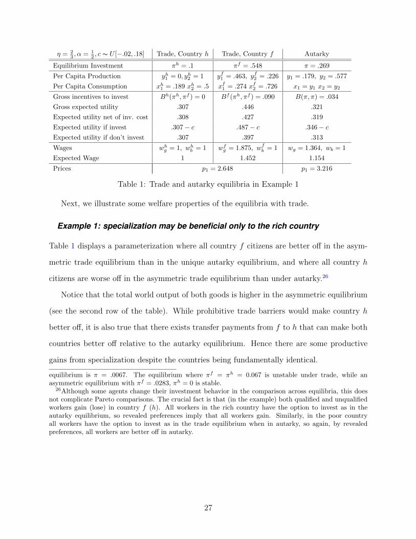
η = 23 , α = 1

2 , c ∼ U [−.02, .18] Trade, Country h Trade, Country f Autarky

Equilibrium Investment πh = .1 πf = .548 π = .269

Per Capita Production yh1 = 0, yh2 = 1 yf1 = .463, yf2 = .226 y1 = .179, y2 = .577

Per Capita Consumption xh1 = .189 xh2 = .5 xf1 = .274 xf2 = .726 x1 = y1 x2 = y2

Gross incentives to invest Bh(πh, πf ) = 0 Bf (πh, πf ) = .090 B(π, π) = .034

Gross expected utility .307 .446 .321

Expected utility net of inv. cost .308 .427 .319

Expected utility if invest .307− c .487− c .346− cExpected utility if don’t invest .307 .397 .313

Wages whg = 1, whb = 1 wfg = 1.875, wfb = 1 wg = 1.364, wb = 1

Expected Wage 1 1.452 1.154

Prices p1 = 2.648 p1 = 3.216

Table 1: Trade and autarky equilibria in Example 1

Next, we illustrate some welfare properties of the equilibria with trade.

Example 1: specialization may be beneficial only to the rich country

Table 1 displays a parameterization where all country f citizens are better off in the asym-

metric trade equilibrium than in the unique autarky equilibrium, and where all country h

citizens are worse off in the asymmetric trade equilibrium than under autarky.26

Notice that the total world output of both goods is higher in the asymmetric equilibrium

(see the second row of the table). While prohibitive trade barriers would make country h

better off, it is also true that there exists transfer payments from f to h that can make both

countries better off relative to the autarky equilibrium. Hence there are some productive

gains from specialization despite the countries being fundamentally identical.

equilibrium is π = .0067. The equilibrium where πf = πh = 0.067 is unstable under trade, while anasymmetric equilibrium with πf = .0283, πh = 0 is stable.

26Although some agents change their investment behavior in the comparison across equilibria, this doesnot complicate Pareto comparisons. The crucial fact is that (in the example) both qualified and unqualifiedworkers gain (lose) in country f (h). All workers in the rich country have the option to invest as in theautarky equilibrium, so revealed preferences imply that all workers gain. Similarly, in the poor countryall workers have the option to invest as in the trade equilibrium when in autarky, so again, by revealedpreferences, all workers are better off in autarky.

27

η = 23 , α = 1

2 , c ∼ U [.04, .24] Trade, Country h Trade, Country f Autarky

Equilibrium Investment πh = 0 πf = .353 π = 0

Production yh1 = 0, yh2 = 1 yf1 = .284, yf2 = .323 y1 = 0, y2 = 1

Consumption xh1 = .107, xh2 = .5 xf1 = .177, xf2 = .823 x1 = y1 x2 = y2

Gross incentives to invest Bh(πh, πf ) = 0 Bf (πh, πf ) = .111 B(π, π) = 0

Gross average utility .232 .381 0

Avg. utility net of inv. cost .232 .355 0

Expected utility if invest .232− c .452− c n/a

Expected utility if don’t invest .232 .342 0

Wages whg = 1, whb = 1 wfg = 2.433, whb = 1 wg = n/a, wb = 1

Expected Wage 1 1.647 1

Prices p1 = 4.660 p1 =n/a

Table 2: Trade and autarky equilibria in Example 2

Example 2: specialization may make both countries better off

In this example trade makes both countries better off. For maximal simplicity we rig this

example so that the “free rider problem” in human capital investments is so severe that

the unique equilibrium under autarky is the trivial equilibrium. However, with trade, the

existence of the other country means that, for any investment πf in country f, the price of

good 1 is higher than without trade if there is no human capital investment in country h.

Hence, trade allows a new market to emerge that would not operate without trade.

Table 2 summarizes one example where the market for good 1 only operates with inter-

national trade. There are multiple trade equilibria and the numbers in the table refer to the

one with the largest fraction of investors in the country producing good 1.27

Consumers are happier when consuming both goods than when consuming only one good.

Because a new market opens up, trade is beneficial for both countries.

Pareto Improving Inequality

The example presented above is extreme, but specialization through trade may more gener-

ally be viewed as an imperfect “solution” to the informational problem.28 In the example,

27(πh, πf ) = (0, 0.0157), is also an equilibrium, but unlike the equilibrium in Table 2 it is unstable.28For a detailed elaboration on this point in the context of discrimination, see Norman (2003).

28

there is no way for a market to open unless the rewards for getting into the market are large

enough. These rewards are bigger if only one country enters the market: the same “kick”

from the local informational externality is generated at a smaller negative price effect. Spe-

cialization reduces the problem of under investment in human capital.

6

-

@@@@@

@@@@@

@@@@@

@@@@@

@@@@@

@@@@@

@@@@@

@@@@@EEEEEEEEE

EEEEEEEEE

EEEEEEEEE

EEEEEEEEE

EEEEEEEEE

EEEEEEEEE

EEEEEEEEE

EEEEEEEEE

EEEEEEEEE

EEEEEEEEE

EEEEEEEEE

EEEEEEEEE

EEEEEEEEE

EEEEEEEEE

EEEEEEEEE

EEEEEEEEE

EEEEEEEEE

EEEEEEEEE

EEEEEEEEE

EEEEEEEEE

EEEEEEEEE

EEEEEEEEE

EEEEEEEEE

EEEEEEEEE

EEEEEEEEE

EEEEEEEEE

EEEEEEEEE

EEEEEEEEE

EEEEEEEEE

EEEEEEEEE

EEEEEEEEE

EEEEEEEEE

EEEEEEEEE

EEEEEEEEE

EEEEEEEEE

EEEEEEEEE

EEEEEEEEE

EEEEEEEEE

EEEEEEEEE

EEEEEEEEE

EEEEEEEEE

EEEEEEEEE

EEEEEEEEE

EEEEEEEEE

EEEEEEEEE

EEEEEEEEE

EEEEEEEEE

EEEEEEEEE

EEEEEEEEE

EEEEEEEEE

EEEEEEEEE

EEEEEEEEE

EEEEEEEEE

EEEEEEEEE

EEEEEEEEE

EEEEEEEEE

EEEEEEEEE

EEEEEEEEE

EEEEEEEEE

EEEEEEEEE

EEEEEEEEE

EEEEEEEEE

EEEEEEEEE

EEEEEEEEE

EEEEEEEEE

EEEEEEEEE

EEEEEEEEE

EEEEEEEEE

EEEEEEEEE

EEEEEEEEE

EEEEEEEEE

EEEEEEEEE

EEEEEEEEE

EEEEEEEEE

EEEEEEEEE

EEEEEEEEE

EEEEEEEEE

EEEEEEEEE

EEEEEEEEE

EEEEEEEEE

EEEEEEEEE

EEEEEEEEE

EEEEEEEEE

EEEEEEEEE

EEEEEEEEE

EEEEEEEEE

EEEEEEEEE

EEEEEEEEE

EEEEEEEEE

EEEEEEEEE

EEEEEEEEE

EEEEEEEEE

EEEEEEEEE

EEEEEEEEE

EEEEEEEEE

EEEEEEEEE

EEEEEEEEE

EEEEEEEEE

EEEEEEEEE

EEEEEEEEE

EEEEEEEEE

EEEEEEEEE

EEEEEEEEE

EEEEEEEEE

EEEEEEEEE

EEEEEEEEE

EEEEEEEEE

EEEEEEEEE

EEEEEEEEE

EEEEEEEEE

EEEEEEEEE

EEEEEEEEE

EEEEEEEEE

EEEEEEEEE

EEEEEEEEE

EEEEEEEEE

EEEEEEEEE

EEEEEEEEE

EEEEEEEEE

EEEEEEEEE

EEEEEEEEE

EEEEEEEEE

EEEEEEEEE

EEEEEEEEE

EEEEEEEEE

EEEEEEEEE

EEEEEEEEE

EEEEEEEEE

EEEEEEEEE

EEEEEEEEE

EEEEEEEEE

EEEEEEEEE

EEEEEEEEE

EEEEEEEEE

EEEEEEEEE

EEEEEEEEE

EEEEEEEEE

EEEEEEEEE

EEEEEEEEE

EEEEEEEEE

EEEEEEEEE

EEEEEEEEE

EEEEEEEEE

EEEEEEEEE

EEEEEEEEE

EEEEEEEEE

EEEEEEEEE

EEEEEEEEE

EEEEEEEEE

EEEEEEEEE

EEEEEEEEE

EEEEEEEEE

EEEEEEEEE

EEEEEEEEE

EEEEEEEEE

EEEEEEEEE

EEEEEEEEE

EEEEEEEEE

EEEEEEEEE

EEEEEEEEE

EEEEEEEEE

EEEEEEEEE

EEEEEEEEE

EEEEEEEEE

EEEEEEEEE

EEEEEEEEE

EEEEEEEEE

EEEEEEEEE

EEEEEEEEE

EEEEEEEEE

EEEEEEEEE

EEEEEEEEE

EEEEEEEEE

EEEEEEEEE

EEEEEEEEE

EEEEEEEEE

EEEEEEEEE

EEEEEEEEE

EEEEEEEEE

EEEEEEEEE

EEEEEEEEE

EEEEEEEEE

EEEEEEEEE

EEEEEEEEE

EEEEEEEEE

EEEEEEEEE

EEEEEEEEE

EEEEEEEEE

EEEEEEEEE

EEEEEEEEE

EEEEEEEEE

EEEEEEEEE

EEEEEEEEE

EEEEEEEEE

EEEEEEEEE

EEEEEEEEE

EEEEEEEEE

EEEEEEEEE

EEEEEEEEE

EEEEEEEEE

EEEEEEEEE

EEEEEEEEE

EEEEEEEEE

EEEEEEEEE

EEEEEEEEE

EEEEEEEEE

EEEEEEEEE

EEEEEEEEE

EEEEEEEEE

EEEEEEEEE

EEEEEEEEE

EEEEEEEEE

EEEEEEEEE

EEEEEEEEE

EEEEEEEEE

EEEEEEEEE

EEEEEEEEE

EEEEEEEEE

EEEEEEEEE

EEEEEEEEE

EEEEEEEEE

EEEEEEEEE

EEEEEEEEE

EEEEEEEEE

EEEEEEEEE

EEEEEEEEE

EEEEEEEEE

EEEEEEEEE

EEEEEEEEE

EEEEEEEEE

EEEEEEEEE

EEEEEEEEE

EEEEEEEEE

EEEEEEEEE

EEEEEEEEE

EEEEEEEEE

EEEEEEEEE

EEEEEEEEE

EEEEEEEEE

EEEEEEEEE

EEEEEEEEE

EEEEEEEEE

EEEEEEEEE

EEEEEEEEE

EEEEEEEEE

EEEEEEEEE

EEEEEEEEE

EEEEEEEEE

EEEEEEEEE

EEEEEEEEE

EEEEEEEEE

EEEEEEEEE

EEEEEEEEE

EEEEEEEEE

EEEEEEEEE

EEEEEEEEE

EEEEEEEEE

EEEEEEEEE

EEEEEEEEE

EEEEEEEEE

EEEEEEEEE

EEEEEEEEE

EEEEEEEEE

EEEEEEEEE

EEEEEEEEE

EEEEEEEEE

EEEEEEEEE

EEEEEEEEE

EEEEEEEEE

EEEEEEEEE

EEEEEEEEE

EEEEEEEEE

EEEEEEEEE

EEEEEEEEE

EEEEEEEEE

EEEEEEEEE

EEEEEEEEE

EEEEEEEEE

EEEEEEEEE

EEEEEEEEE

EEEEEEEEE

EEEEEEEEE

EEEEEEEEE

EEEEEEEEE

EEEEEEEEE

EEEEEEEEE

EEEEEEEEE

EEEEEEEEE

EEEEEEEEE

EEEEEEEEE

EEEEEEEEE

EEEEEEEEE

EEEEEEEEE

EEEEEEEEE

EEEEEEEEE

EEEEEEEEE

EEEEEEEEE

EEEEEEEEE

EEEEEEEEE

EEEEEEEEE

EEEEEEEEE

EEEEEEEEE

EEEEEEEEE

EEEEEEEEE

EEEEEEEEE

EEEEEEEEE

EEEEEEEEE

EEEEEEEEE

EEEEEEEEE

EEEEEEEEE

EEEEEEEEE

EEEEEEEEE

EEEEEEEEE

EEEEEEEEE

EEEEEEEEE

EEEEEEEEE

EEEEEEEEE

EEEEEEEEE

EEEEEEEEE

EEEEEEEEE

EEEEEEEEE

EEEEEEEEE

EEEEEEEEE

EEEEEEEEE

EEEEEEEEE

EEEEEEEEE

EEEEEEEEE

EEEEEEEEE

EEEEEEEEE

EEEEEEEEE

EEEEEEEEE

EEEEEEEEE

EEEEEEEEE

EEEEEEEEE

EEEEEEEEE

EEEEEEEEE

EEEEEEEEE

EEEEEEEEE

EEEEEEEEE

EEEEEEEEE

EEEEEEEEE

EEEEEEEEE

EEEEEEEEE

EEEEEEEEE

EEEEEEEEE

EEEEEEEEE

EEEEEEEEE

EEEEEEEEE

EEEEEEEEE

EEEEEEEEE

EEEEEEEEE

EEEEEEEEE

EEEEEEEEE

EEEEEEEEE

EEEEEEEEE

EEEEEEEEE

EEEEEEEEE

EEEEEEEEE

EEEEEEEEE

EEEEEEEEE

EEEEEEEEE

EEEEEEEEE

EEEEEEEEE

EEEEEEEEE

EEEEEEEEE

EEEEEEEEE

EEEEEEEEE

EEEEEEEEE

EEEEEEEEE

EEEEEEEEE

EEEEEEEEE

EEEEEEEEE

EEEEEEEEE

EEEEEEEEE

EEEEEEEEE

EEEEEEEEE

EEEEEEEEE

EEEEEEEEE

EEEEEEEEE

EEEEEEEEE

EEEEEEEEE

EEEEEEEEE

EEEEEEEEE

EEEEEEEEE

EEEEEEEEE

EEEEEEEEE

EEEEEEEEE

EEEEEEEEE

EEEEEEEEE

EEEEEEEEE

6

-

@@@@@@@@@@@@@@@@@@s s ssB A C

D

A

E

s

s

x2

x1

x2

x1π − k πkπ + k

Figure 9: Specialization expands the world production possibilities

Even in less extreme cases, both countries may gain from specializing: it is always true

that the production possibilities set expands when moving from a situation where both

countries invest at the same rate to an asymmetric investment profile for a constant total

quantity of investors in the world. Figure 9 assumes countries of equal size. In the left

panel, the dashed line represents the frontier when both countries invest at π, whereas

the continous lines (with kinks at B and C) illustrate the frontiers in each country at an

asymmetric investment profile, but with the same aggregate investment.

On the right panel the continuous line (with kinks at D,A and E) is the world production

possibilities frontier under the same asymmetric investment profile assumed in the left panel.

The dashed line reproduces the dashed line from the left panel. The total number of investors

in the world is unchanged, but the world production possibilities set is larger when countries

specialize. To understand, note that the efficient way of increasing x1 starting from the

vertical intercept is to first use good-signal workers from the country with higher investment,

so initially the slope of the world production possibilities set must be the same as the set to

the left with kink at C. The graph is drawn for the case where it is better to use high-signal

29

workers from the low investment country than low signal workers from the high investment

country in Sector 1, but the result is fully general.

The Irrelevance of Size

Changes of the relative size of the countries will in general affect the asymmetric equilibria

due to price effects. The nature of such changes depends on the parameterization.

To illustrate that size does not confer special advantage as it does in agglomeration

models, we construct examples showing that scale effects may go either way. One way

is to look at the extreme case where λh is near zero (see Appendix B for details on the

computation). In this case the foreign (big) country operates as in autarky. In the (small)

home country instead, price effects are absent, because world price is only determined by

investment in the the foreign country. The examples are computed by setting λh = 1

Figure 10 panel (A) was computed using α = 1/2, η = .97, c = −0.005, c = .095 to

illustrate one case where only the big country can be rich. There is a unique symmetric

equilibrium at πA = 0.48. At the autarky equilibrium, incentives to invest in human capital

are decreasing in π in the large country. In the small country instead, additional investment

does not have adverse price effects, and incentives BO increase with π, but not at a fast

enough rate: the best response for the small country G(BO(π, p = pA)) intersects the 450

line only below πA. Therefore there are two asymmetric equilibria where the big country

invests at πh = πA = 0.48 and the other at πf = 0.05 or 0.29, both less than πA.

In the example of Figure 10 panel (B) instead, the small country can be either richer or

poorer than the big country. The figure was computed with the parameters as in Numerical

Example 1 (except for country sizes). Workers’ investment in the small country is more

responsive than in the previous example at the autarky equilibrium, where the best response

intersects the 450 line from below. Both(πh, πf

)= (.27, 0.1) and

(πh, πf

)= (.27, 0.59) are

equilibria. Note that the responsiveness of the best-response function to higher investment,

which determines the location of the fixed points for the small country above and below

πA also depends on the shape of cost of investment distribution, therefore, by changing the

30

1

0.05

0.29

0.48

1.

0 1

0.1

0.27

0.59

1

Figure 10: Equilibrium fixed point maps: large (solid line) and small (dashed line) country

shape of the cost distribution one can easily construct examples where differences between

countries are large or small regardless of country size.

Finally, when the unique autarky equilibrium is at πA = 0, if the large country is large

enough only the small country can be richer. For example, if Example 2 above is extended

to allow for different country sizes, the country must fully specialize in the low-tech industry

if its size exceeds a critical value. Reducing the size of the country from 1/2 on the other

hand only improves incentives. Hence, there are circumstances where the only asymmetric

equilibrium is that the small country becomes rich.

Taken together, these examples show that there may be scale effects in favor of either

the larger or the smaller economy, and that sometimes the equilibrium selection matters.

However, these are not really “country-scale-effects”. Instead, we prefer to think of them as

scale effects that depend on relative size of the North to the South. To understand, suppose

that there are n countries indexed by j ∈ {1, ..., n} , of size λj. Consider an equilibrium in

this model where the set of countries is partitioned into the sets P and R and where πj = πp

for all j ∈ P and πj = πr for all j ∈ R. Finally let λp =∑

j∈P λj and λr =

∑j∈R λ

j. This

is an equilibrium if and only if (πp, πr) is an equilibrium in the two-country model with

countries of sizes (λp, λr). There may of course be other equilibria as well, but at least for

this form of equilibrium the size of the individual country is irrelevant and the relevant scale

effect can be interpreted in our preferred manner.

31

A “development miracle” can be interpreted as a country that re-coordinates from being

part of the developing world to being part of the developed world. The model cannot explain

how such a re-coordination is achieved, but, if the economy is small, the effects on the rest of

the world are negligible. In contrast, a simultaneous re-coordination of a significant fraction

of the “South” leads to large relative price changes so that it is not worth the while as

long as there is no change in the “North”. Obviously, the model is too stylized for policy

recommendations, but this nevertheless suggests that it may be misguided to use a few small

successful countries as a model for all developing countries.

VII Concluding Remarks

We show that endogenous comparative advantages are possible between identical countries

in an essentially neoclassical model. Specialization and trade arise due to an informational

externality: workers are better informed than firms about their abilities.

Two-country model equilibria can be reinterpreted as n-country model equilibria where

countries cluster in two groups in terms of level of development. Equilibria of the n-country

model are neutral with respect to individual country sizes, so the model is consistent with a

world with no particular relationship between size and development.

A natural extension is to introduce physical capital into the production technology. This

would be interesting for analyzing the role of foreign capital and capital flight from poor

countries. As this paper focuses on the effects asymmetric information about skills we have

chosen to ignore physical capital. However, if capital and human capital were complementary

in production, the effects analyzed in this paper would be reinforced.

To understand, suppose initially that capital cannot flow between countries. Except

for a capital market equilibrium condition the model is more or less the same as the one

without capital. Consider an asymmetric equilibrium under the assumption that initial

capital endowments are identical. As capital is more useful in the high-tech industry the

return on capital is higher in the rich country, so, with free capital mobility, the rich country

32

must have a higher per capita level of capital. Notice that the movement of capital from

the poor to the rich country affects incentives to invest positively in the rich country and

negatively in the poor country, strengthening the incentives to specialize.29

Because this is a static model, we do not analyze incentives to migrate. Workers with

good signals in poor countries may find it advantageous to migrate where their skills receive

better rewards. However, such incentives are mitigated if employers recognize the workers’

country of origin. When a foreign employer forms beliefs about a home country worker’s

productivity, she may take into account the worker’s nationality, therefore the expected

productivity computed by foreign and home country employers is the same. Then, incentives

to acquire human capital are defined by citizenship, not residence.30

A Appendix: Proof of proposition 1.

(Part 1) Consider an arbitrary equilibrium. Let x∗ = (x∗1, x∗2) denote the world production,

where x∗i = λhxh∗i + λfxf∗i and xj∗i denotes the production of good i in country j in equilib-

rium. Also let lj∗i (θ) denote the corresponding input of workers with signal g in economy j

and sector i. By profit maximization p∗ixj∗i −∑

θ∈g,bwj∗θ l

j∗i (θ) ≥ p∗ix

j′i −∑

θ∈g,bwj∗θ l

j′i (θ) for any

alternative plan (xj′i , lj′i (·)). Adding over the two sectors and imposing the market clearing

conditions on the labor market we conclude that∑

i=1,2 p∗ix

j∗i −wj∗g (ηπj + (1− η) (1− πj))−

wj∗b ((1− η) πj + η(1− πj)) ≥∑

i=1,2 p∗ix

j′i − wj∗g

(lj1 (g) + lj2 (g)

)− wj∗b

(lj1 (b) + lj2 (b)

)for all

possible alternative production plans (feasible as well as non-feasible in the aggregate).

Now for any feasible alternative allocation lj1 (g) + lj2 (g) ≤ ηπj + (1− η) (1 − πj) and

lj1 (b) + lj2 (b) ≤ (1− η) πj + η(1− πj), implying that∑

i=1,2 p∗ix

j∗i ≥

∑i=1,2 p

∗ix

j′i for any fea-

sible alternative (xj′1 , xj′2 ). Since this must hold in each country we conclude that p∗x∗ ≥ p∗x′

for any alternative feasible world production vector x′ = (x′1, x′2) . Moreover, in order for

29Details are available on request from the authors.30However, employers may also condition their beliefs on migration status, which is as easily recognizable

as citizenship. This raises the possibility that migrants acquire a reputation for higher investment than theirfellow citizens who did not migrate, and that this belief is confirmed in equilibrium.

33

(xj∗1 , xj∗2 ) to be profit maximizing it must be that

∑i=1,2 p

∗ix

j∗i −wj∗g (ηπj + (1− η) (1− πj))+

wj∗b ((1− η) πj + η(1− πj)) = 0. Finally, since u is homothetic, from standard arguments we

have that if (xj∗1 (w) , xj∗2 (w)) maximizes utility of a worker with income w, then (w′

wxj∗1 (w) , w

′

wxj∗2 (w))

maximizes utility of a worker with income w′. Consider the program

maxx1,x2

u (x1, x2) (A1)

s.t p∗1x1 + p∗2x2 ≤ p∗1x∗1 + p∗2x

∗2 = p∗1

∑j=h,f

λjxj∗1 + p∗2∑j=h,f

λjxj∗2 ,

where the star-superscript refers to equilibrium variables. The aggregate consumption bundle

of any equilibrium must solve (A1) because the problem gets the relative consumptions of

x1 and x2 right and p∗1x∗1 + p∗2x

∗2 is the aggregate world income. We conclude that if x∗

is an equilibrium world consumption plan it must solve (A1). Since the set XW(πh, πf

)is contained in the “budget set” of the representative consumer and x∗ ∈ XW

(πh, πf

)it

follows that x∗ must be a solution to (12).

(Part 2) Let x∗ solve (12) and let V ={x ∈ R2

+|u (x) > u (x∗)}

. Quasi-concavity implies

that V is a convex set. The set XW(πh, πf

)is also convex (see Page 13). Moreover,

V ∩XW(πh, πf

)= ∅, so the separating hyperplane theorem (Theorem 11.3. in Rockafellar

(1997)) implies that there exists some p∗ such that p∗x ≥ p∗x∗ for all x ∈ V and p∗x ≤ p∗x∗

for every x ∈ XW(πh, πf

). Let the wages be given by wj∗g = max {p∗1µ (g, πj) , p∗2} and

wj∗b = max {p∗1µ (b, πj) , p∗2}, and let the allocation of workers be as in the planning solution.

Observe in particular that if p∗1µ (θ, πj) > p∗2, then no worker with signal θ is employed in

Sector 2 in the allocation that produces x∗. This is most easily seen in the differentiable case,

where the optimality condition to (12) implies that ∂u(x∗)∂x∗1

/∂u(x∗)∂x∗2

=p∗1p∗2> 1

µ(g,πj). But, 1

µ(θ,πj)is

the cost of producing an extra unit of good 1 by giving up some country j workers with good

signal currently in production of good 2, so we conclude that as if representative consumer

would be better off if some of these workers would be switched to the production of good

1, contradicting optimality of x∗ if p∗1µ (θ, πj) > p∗2 and some of the j workers are assigned

to Sector 2. A symmetric argument holds for when the inequality is reversed. Hence, if

l∗j1 (θ) > 0, then p∗1µ (θ, πj) = max {p∗1µ (θ, πj) , p∗2} = wj∗θ , implying that the profit from

34

hiring any quantity workers with signal θ is zero in Sector 1, whereas if l∗j1 (θ) = 0, then

p∗1µ (θ, πj) ≤ max {p∗1µ (θ, πj) , p∗2} = wj∗θ , so no gain can be earned from hiring a positive

quantity. The argument for Sector 2 is symmetric, which leads us to conclude that the

outputs and (implicit) allocation of workers in the solution to (12) are consistent with profit

maximizing behavior given the prices and wages constructed.

B Appendix: Equilibria when One Country is a Small Open Econ-

omy

Equilibria can be calculated by solving two separate (different) one-dimensional fixed point

problems. Consider the incentives to invest in a country with fraction of investors π under the

“small open economy” assumption that the price (of good 1) is fixed at p. Equilibrium wages

in the small open economy are determined to generate zero profits: wOg = max {pµ (g, π) , 1}

and wOb = max {pµ (b, π) , 1}. The incentive to invest in the small open economy, denoted

BO (π; p) , is thus (using (15)),

BO (π; p) =(2η − 1)αα(1− α)1−α

pαmax {max{pµ (g, π) , 1} −max {pµ (b, π) , 1} , 0} . (B2)

If pA is well defined (i.e., whenever the autarky equilibrium is non-trivial), then

Bh(πh, πA

)→ BO

(πh, p = pA

)for all πh ∈ [0, 1] as λh → 0 (B3)

Bf(πh, πA

)→ B

(πf)

for all πf ∈ [0, 1] as λh → 0,

Assume parameters imply a unique autarky equilibrium, and call it πA. Let pA denote

the associated autarky price. If π = πA, then BO(πA; p = pA

)= B

(πA), and πA solves

π = G(BO(π; p = pA

)). (B4)

While both (B4) and the autarky fixed point equation have πA as a common solution,

incentives diverge for other values of π since in autarky the price changes as π changes whereas

there are no such price effects in (B2). Equation (B4) will therefore in many cases have

solutions different from πA. Now, if πO solves (B4) and if ddπ

∣∣π=πA [π −G (B (π))] 6= 0 and

35

ddπ

∣∣π=πO

[π −G

(BO(π; p = pA

))]6= 0, then, for λh small enough, there exists an equilibrium(

πh∗, πf∗)

in the trade model near(πO, πA

).31

References

Altonji, Joseph G. and Charles R. Pierret (2001), Employer Learning and Statistical Dis-

crimination, The Quarterly Journal of Economics 116, 313–350.

Araujo, Luis F. and Emanuel Ornelas (2007), Trust-Based Trade, SSRN working paper

n.642803.

Araujo, Luis, Giordano Mion, and Emanuel Ornelas (2016), Institutions and Export Dy-

namics, Journal of International Economics 98, 2–20.

Auer, Raphael A. (2015), Human Capital and the Dynamic Effects of Trade, Journal of

Development Economics 117, 107–118.

Basu, Arnab K and Nancy Chau (1998), Asymmetric Country-of-Origin Effects on Intrain-

dustry Trade and the International Quality Race, Review of Development Economics 2,

140–166.

Blanchard, Emily and Gerald Willmann (2016), Trade, Education, and the Shrinking Middle

Class, Journal of International Economics 99, 263–278.

Bonfatti, Roberto and Maitreesh Ghatak (2013), Trade and the Allocation of Talent with

Capital Market Imperfections, Journal of International Economics 89, 187–201.

Bougheas, Spiros, Richard Kneller, and Raymond Riezman (2011), Optimal Education Poli-

cies and Comparative Advantage, Pacific economic review 16, 538–552.

Cartiglia, Filippo (1997), Credit Constraints and Human Capital Accumulation in the Open

Economy, Journal of International Economics 43, 221–236.

Casella, Alessandra and James E. Rauch (2002), Anonymous Market and Group Ties in

International Trade, Journal of International Economics 58, 19–47.

31The slope condition for the autarky equilibrium is satisfied under the conditions that guarantee theequilibrium uniqueness. Its role is that if the equilibrium was at a tangency with the 450 line, the slightesteffect from abroad could eliminate the equilibrium.

36

Chatterjee, Arpita (2017), Endogenous Comparative Advantage, Gains From Trade and

Symmetry-Breaking, Journal of International Economics 109.

Chisik, Richard (2003), Export Industry Policy and Reputational Comparative Advantage,

Journal of International Economics 59, 423–451.

Coate, Stephen and Glenn C. Loury (1993), Will Affirmative-Action Policies Eliminate Neg-

ative Stereotypes?, The American Economic Review 83, 1220–1240.

Cornwell, Christopher, Jason Rivera, and Ian M. Schmutte (2017), Wage Discrimination

when Identity is Subjective: Evidence from Changes in Employer-Reported Race, Journal

of Human Resources 52, 719–755.

Costinot, Arnaud (2009), On the Origins of Comparative Advantage, Journal of Interna-

tional Economics 77, 255–264.

Creane, Anthony and Thomas D. Jeitschko (2016), Shipping The Good Apples Out Under

Asymmetric Information: When Weak Institutions Lead to Welfare-Diminishing Trade,

European Economic Review 85, 246–262.

Danziger, Eliav (2017), Skill Acquisition and the Dynamics of Trade-Induced Inequality,

Journal of International Economics 107, 60–74.

Davidson, Carl and Nicholas Sly (2014), A Simple Model of Globalization, Schooling and

Skill Acquisition, European Economic Review 71, 209–227.

Eicher, Theo S. (1999), Training, Adverse sSlection and Appropriate Technology: Develop-

ment and Growth in a Small Open Economy, Journal of Economic Dynamics and Control

23, 727–746.

Ethier, Wilfred J (1982), Decreasing Costs in International Trade and Frank Graham’s Ar-

gument for Protection, Econometrica 50, 1243–1268.

Falvey, Rod, David Greenaway, and Joana Silva (2010), Trade Liberalisation and Human

Capital Adjustment, Journal of International Economics 81, 230–239.

Farber, Henry S. and Robert Gibbons (1996), Learning and Wage Dynamics, The Quarterly

Journal of Economics 111, 1007–1047.

37

Findlay, Ronald and Henryk Kierzkowski (1983), International Trade and Human Capital:

a Simple General Equilibrium Model, The Journal of Political Economy 91, 957–978.

Grossman, Gene M. (2004), The Distribution of Talent and the Pattern and Consequences

of International Trade, Journal of Political Economy 112, 209–239.

Grossman, Gene M. and Giovanni Maggi (2000), Trade and Diversity, The American Eco-

nomic Review 90.

Harris, Richard G. and Peter E. Robertson (2013), Trade, Wages and Skill Accumulation in

the Emerging Giants, Journal of International Economics 89, 407–421.

Kahn, Lisa B. and Fabian Lange (2014), Employer Learning, Productivity, and the Earnings

Distribution: Evidence from Performance Measures, The Review of Economic Studies 81,

1575–1613.

Krugman, Paul (1980), Scale Economies, Product Differentiation, and the Pattern of Trade,

The American Economic Review 70, 950–959.

Krugman, Paul and Anthony J. Venables (1995), Globalization and the Inequality of Nations,

The Quarterly Journal of Economics 110, 857–880.

Lange, Fabian (2007), The Speed of Employer Learning, Journal of Labor Economics 25,

1–35.

Lesner, Rune V. (2017), Testing for Statistical Discrimination Based on Gender, LABOUR

Online version: doi:10.1111/labr.12120.

Matsuyama, Kiminori (1996), Why Are There Rich and Poor Countries? Symmetry-

Breaking in the World Economy, Journal of the Japanese and International Economies

10, 419–439.

(2002), Explaining Diversity: Symmetry-Breaking in Complementarity Games,

American Economic Review Papers and Proceedings, 241–246.

(2004), Financial Market Globalization, Symmetry-Breaking, and Endogenous In-

equality of Nations, Econometrica 72, 853–884.

McCalman, Phillip (2002), Multi-lateral Trade Negotiations and the Most Favored Nation

38

Clause, Journal of International Economics 57, 151–176.

Moro, Andrea and Peter Norman (2004), A General Equilibrium Model of Statistical Dis-

crimination, Journal of Economic Theory 114, 1–30.

Norman, Peter (2003), Statistical Discrimination and Efficiency, The Review of Economic

Studies 70, 615–627.

Park, Jee-Hyeong (2011), Enforcing International Trade Agreements with Imperfect Private

Monitoring, The Review of Economic Studies 78, 1102–1134.

Pinkston, Joshua C. (2009), A Model of Asymmetric Employer Learning with Testable Im-

plications, The Review of Economic Studies 76, 367–394.

Puga, Diego and Anthony J. Venables (1999), Agglomeration and Economic Development:

Import Substitution vs. Trade Liberalisation, The Economic Journal 109, 292–311.

Ranjan, Priya (2001), Dynamic Evolution of Income Distribution and Credit-Constrained

Human Capital Investment in Open Economies, Journal of International Economics 55,

329–358.

Rasmusen, Eric (2017), A Model of Trust in Quality and North–South Trade, Research in

Economics 71, 159–170.

Razin, Assaf and Efraim Sadka (2003), Gains from FDI Inflows with Incomplete Information,

Economics Letters 78, 71–77.

Rockafellar, R. Tyrrell (1997) Convex Analysis. Princeton Landmarks in Mathematics :

Princeton University Press, Princeton, NJ.

Schonberg, Uta (2007), Testing for Asymmetric Employer Learning, Journal of Labor Eco-

nomics 25, 651–691.

Unel, Bulent (2015), Human Capital Formation and International Trade, The BE Journal

of Economic Analysis & Policy 15, 1067–1092.

Vogel, Jonathan (2007), Institutions and Moral Hazard in Open Economies, Journal of

International Economics 71, 495–514.

Zhang, Xin (2012), Credit Constraints and Decisions in Exports: Theory under Asymmetric

39

Information, Journal of Mathematical Finance 2, p. 238.

40