1

Área 4 - Macroeconomia, Economia Monetária e Finança

Endogeneity and nonlinearities in Central Bank of Brazil’s reaction functions: an

inverse quantile regression approach

Gabriela Bezerra de Medeiros

Professora do Departamento de Economia da Universidade Federal da Paraíba, Brasil

E-mail: gabriela.bm@hotmail.com

Marcelo Savino Portugal

Professor do Programa de Pós-Graduação em Economia da Universidade Federal do Rio Grande do Sul

(PPGE/UFRGS) e pesquisador CNPq, Brasil

E-mail: msp@ufrgs.com

Edilean Kleber da Silva Bejarano Aragón

Professor do Departamento de Economia e do Programa de Pós-Graduação em

Economia da Universidade Federal da Paraíba (PPGE/UFPB), Brasil

E-mail:edilean@hotmail.com

Resumo: Neste trabalho, nós procuramos averiguar não linearidades na função de reação do Banco

Central do Brasil (BCB) através da estimação de regressões quantílicas. Como a regra de política

monetária apresenta regressores endógenos, nós seguimos os procedimentos sugeridos por Wolters (J

Macroecon 34:342-361, 2012) e um estimador de regressão quantílica inversa (RQIV), proposto por

Chernozhukov e Hansen (Econometrica 73:245–261, 2005). Este método nos possibilitou detectar não

linearidades na função de reação do BCB sem a necessidade de fazer suposições específicas acerca dos

fatores que determinam essas não linearidades. Em específico, nós observamos que: i) a resposta da taxa

de juros ao hiato da inflação corrente e esperada foi, em geral, mais forte na parte superior da distribuição

condicional da taxa de juros Selic; ii) a resposta ao hiato do produto apresentou uma tendência crescente e

significativa na parte inferior da distribuição condicional da taxa Selic; iii) a resposta do BCB à taxa de

câmbio real foi positiva e mais elevada na cauda superior da distribuição condicional da taxa Selic.

Palavras-chave: Regras de política monetária ∙ Regressão quantílica ∙ Regressores endógenos ∙ Banco

Central do Brasil.

Abstract: In this work, we seek to investigate nonlinearities in the reaction function of the Central Bank

of Brazil by estimating quantile regressions. As the monetary policy rule has endogenous regressors, we

followed the procedures suggested by Wolters (J Macroecon 34:342-361, 2012) and the method of

inverse quantile regression, proposed by Chernozhukov and Hansen (Econometrica 73:245–261, 2005).

This method enabled us to detect nonlinearities in the Central Bank of Brazil’s reaction function without

the need to make specific assumptions about the factors that determine these nonlinearities. In particular,

we observed that: i) the response of the interest rate to the current and expected inflation was, in general, stronger in the upper tail of the conditional interest rate distribution; ii) the response to the output gap

showed a growing and significant trend in the lower tail of the conditional Selic rate distribution; iii) the

response of the Central Bank of Brazil to the real exchange rate was positive and higher in the upper tail

of the conditional Selic rate distribution.

Keywords: Monetary policy rules ∙ Quantile regression ∙ Endogenous regressors ∙ Central Bank of Brazil.

JEL Classification C32 ∙ E52 ∙ E58

2

1 Introduction

The inflation-targeting regime was adopted by the Central Bank of Brazil (CBB) in July 1999. This

decision was taken six months after the transition from an exchange rate band system to a floating system.

Owing to exchange rate overshooting and to the rise in inflation and in inflation expectations, the

Brazilian government aimed to implement a policy regime that was institutionally committed to

maintaining price stability and providing a new nominal exchange rate anchor for inflation.

For the analysis of the CBB’s monetary policy decisions in the inflation-targeting regime, several

papers have estimated the Taylor (1993) rule or the forward-looking reaction function proposed by

Clarida et al. (2000).1 For instance, Minella et al. (2003) and Minella and Souza-Sobrinho (2013)

estimated a forward-looking reaction function and observed that the CBB strongly reacted to inflation

expectations. Mello and Moccero (2009) utilized cointegration analysis and M-GARCH model

estimations to check for the presence of long-term relationships between the monetary policy interest rate

(Selic rate), inflation expectations, and inflation target, and to verify the presence of volatility spillovers

between inflation expectations and monetary policy. For Brazil, the results gathered by these authors

revealed there exist long-term relationships between the interest rate, expected inflation, and inflation

target, and that higher volatility in monetary policy increases the volatility of the expected inflation.

Sanches-Fung (2011) estimated reaction functions for the CBB in a data-rich environment. Sanches-

Fung’s (2011) evidence points out that the CBB adjusted the Selic interest rate according to the Taylor

principle, but that it did not react systematically to the exchange rate behavior.

An important assumption of the papers mentioned above is that interest rate rules are linear

functions relative to the variables describing economic conditions. By contrast, the economic literature

has come up with numerous reasons why the monetary authority responds nonlinearly to inflation and/or

to the output gap. Nobay and Peel (2000), Schaling (2004) and Dolado et al. (2005) demonstrate that an

optimal nonlinear monetary rule emerges when the central bank has a quadratic loss function and the

Phillips curve is nonlinear. Bec et al. (2002), Nobay and Peel (2003), Dolado et al. (2004), Surico (2007)

and Cukierman and Muscatelli (2008) show nonlinearities in the optimal monetary rule may arise if the

monetary authority’s preferences are asymmetric in relation to inflation and/or to the output gap. By

assessing an optimal monetary policy in an economy where the central bank is uncertain over the Phillips

curve slope, Tillmann (2011) evidences that the interest rate adjustment is nonlinear. Lastly, the zero

lower bound for the nominal interest rate can prompt the central bank to respond nonlinearly to the

inflation rate (Kato and Nishiyama, 2005; Adam and Billi, 2006).2

For Brazil, studies on nonlinearities in the monetary policy rule assess specific features of the

CBB’s asymmetric reaction. For example, Aragón and Portugal (2010), Sá and Portugal (2011) and

Aragón and Medeiros (2013) reveal that the Brazilian monetary authority had an asymmetric preference

for an above-target inflation in the inflation-targeting regime. Moura and Carvalho (2010) find empirical

evidence of nonlinearities in the reaction function that corroborates the CBB’s asymmetric preference

concerning inflation. Lopes and Aragón (2014) describe that the nonlinearity in the interest rate rule

stems from time-varying asymmetric preferences rather than from possible nonlinearities in the Phillips

curve. Schiffino et al. (2013) show that the nonnegativity constraint on the Selic interest rate may affect

the calibration of the CBB’s preferences, implying nonlinearities in the optimal monetary rule. Aragón

and Medeiros (2014) estimate a reaction function whose parameters vary over time and conclude that the

reaction of the Selic rate to inflation varies remarkably throughout the period, showing a downtrend during the inflation-targeting regime.

Unlike the afore-mentioned studies, the present paper seeks to verify nonlinearities in the CBB’s

reaction function by quantile regression estimation. An important advantage of this approach over

1 According to the monetary rule proposed by Taylor (1993), the central bank changes the nominal interest rate in response to

deviations of the current inflation from the inflation target and to the current output gap. In turn, the policy rule formulated by

Clarida et al. (2000) assumes the monetary authority adjusts the interest rate based on expected future inflation rates and on the

output gap. 2 Kato and Nishiyama (2005) and Adam and Billi (2006) argue that, close to the zero bound, the central bank responds more

strongly to a decrease in inflation rate in order to minimize the likelihood of deflation.

3

conventional methods (e.g., least ordinary squares (OLS) and instrumental variables (IV)) is that it allows

estimating the Selic interest rate rule across different quantiles of the conditional interest rate distribution

and not only in the conditional mean of this variable. This permits detecting nonlinearities in the CBB’s

reaction function without having to make specific inferences about the causal factors of these

nonlinearities. Thus, as nonlinearity is determined by the data, the quantile regression method allows

comparing the estimates of the monetary rule parameters obtained for the quantiles of the conditional

interest rate distribution with the mean from the linear reaction function.

Empirically, we used inverse quantile regression (IVQR), proposed by Chernozhukov and Hansen

(2005, 2006), to estimate the CBB’s quantile reaction function parameters during the inflation-targeting

regime. This method was chosen because of the presence of endogenous regressors (inflation rate and

output gap) in the interest rate rule. Some authors, such as Chevapatrakul et al. (2009), Wolters (2012),

and Chevapatrakul and Paez-Farrell (2014), estimate the reaction function by quantile regression. To add

the presence of endogeneity, Chevapatrakul et al. (2009) and Chevapatrakul and Paez-Farrell (2014)

apply the two-stage quantile regression (2SQR) method, while Wolters (2012) uses IVQR.3 Note that

IVQR is a good alternative to the 2SQR method because: i) it yields consistent and unbiased estimates of

all parameters in the model; and ii) the estimates are consistent even when endogenous regressors change

the distribution of the dependent variable (Wolters, 2012).4

The IVQR estimation results for the CBB’s reaction function can be summarized as follows.

While conditional mean estimations showed an insignificant response of the Selic rate to the current

inflation gap, quantile regression results indicated that the CBB’s short-term response to this variable was

significant and increasing between quantiles 0.5 and 0.9. Conversely, the short-term response of the Selic

rate to the output gap increased from quantile 0.2 to quantile 0.7 and was not statistically different from

zero at the extreme quantiles of the conditional interest rate distribution. We also perceived that the short-

term response of the Selic rate to expected inflation was significant from quantile 0.4, exhibiting an

uptrend. Regarding the long-term response, results suggest the Selic rate responded strongly to current

and expected inflation when the interest rate was above the median. On the other hand, the long-term

response to the output gap was significant only at some quantiles on the [0.05, 0.7] interval. This suggests

that the CBB does not react to demand pressures when the interest rate is too high. When we included the

real exchange rate as an interest rate rule regressor, we noticed the CBB responded positively to the real

exchange rate both in the conditional mean and across the interest rate distribution. Moreover, results

show that the reaction to the real exchange rate was, in general, stronger in the upper tail of the

conditional Selic rate distribution.

Aside from this introduction, this paper is organized into four sections. Section 2 describes the

empirical specifications of the CBB’s reaction function and its estimation method across different

quantiles of the conditional interest rate distribution. Section 3 interprets the results. Section 4 concludes.

2 Empirical specifications

In this section, we initially introduce the CBB’s reaction function to be estimated in the conditional mean

of the interest rate. This specification of the policy rule can be derived from the optimal policy problem in

a standard New Keynesian model. Thereafter, we describe the monetary policy rule to be estimated by

quantile regression and the estimation method for this function. Finally, we take into consideration an

alternative specification of the CBB’s reaction function.

3 Chevapatrakul et al. (2009) assess monetary policy conduct in the United States and in Japan, whereas Chevapatrakul and

Paez-Farrell (2014) focus their analysis on Australia, Canada, and New Zealand. In turn, Wolters (2012) estimates the Federal

Reserve’s reaction function. 4 For further details on the 2SQR method, see Amemiya (1982), Powell (1983) and Kim and Muller (2004, 2008).

4

2.1 The monetary policy rule in the conditional mean

Initially, we assumed that CBB monetary policy decisions could be describe by the following reaction

function, estimated on the interest rate conditional mean:

*

1 2 0 1 1 2 1 1 1 2 2(1 ) ( )t t t t t t t t ti E E y i i m

(1)

where it is the nominal interest rate, πt is the inflation rate, π*t is the inflation target, yt is the output gap

(i.e., the difference between actual output and potential output), Et-1(xt) is the expectation of xt conditional

on the information available at the end of the previous period and mt is the exogenous random shock for

the interest rate. This shock is assumed to be i.i.d and can be interpreted as the monetary policy’s purely

random component. Note that we consider a variable inflation target. This is necessary because the

inflation targets established by the Brazilian National Monetary Council varied annually in the period

1999-2004. Finally, we also included it-1 and it-2 in the reaction function to capture the CBB soothing

behavior and to avoid possible serial autocorrelation problems.5

For estimation purposes, the expected values for inflation and output gap in (1) are replaced with

their observed values. By making these amendments, the specification of the policy rule to be estimated is

given by:

*

0 1 2 1 1 2 2( )t t t t t t ti y i i (2)

where β′i = (1 – θ1 – θ2) βi, i=0,1,2, and 1, 1 2, 1( ( )) ( ( ))t t t t t t t t t tE y E y m . The coefficients

β′1 and β′2

(β1 and β2) measure the short-term (long-term) response of the interest rate to inflation and to

output gap.

Once inflation and output gap forecast errors are an integral part of term εt, πt and yt are correlated

with this error term. In view of that, (2) in the conditional mean of the monetary policy’s interest rate will

be estimated by IV and by the generalized method of moments (GMM).

2.2 The monetary policy rule across different conditional quantiles

Quantile regression models manage to determine the heterogeneous impacts of variables at different

points along a distribution. Quantile regression was first proposed by Koenker and Bassett (1978) and

has rather attractive features, namely: i) it can be used to assess the response of the dependent variable to

explanatory variables at different points of the dependent variable distribution; ii) quantile regression

estimators are more efficient than OLS estimators when the error term is non-Gaussian; and iii) quantile

regression estimators are less sensitive to the presence of outliers in the dependent variable (Koenker,

2005).

Quartiles split observations into four segments with equal proportions of benchmark observations

in each segment. Quintiles and deciles, similarly to quartiles, split observations into 5 and 10 segments,

respectively. Quantiles or percentiles refer to the general case (Koenker and Hallock, 2001). For our

monetary policy problem, the τth conditional quantile is defined as qτ (it | it-1, it-2, πt – π*t , yt) such that the

likelihood of the nominal interest rate being smaller than qτ (it | it-1, it-2, πt – π*t , yt) is equal to τ, i.e.:

*1 2

*1 2

| , , ,*

1 2| , , ,| , , , , (0,1)

t t t t t t

t t t t t t

q i y i i

t t t t t ti y i if i y i i di

(3)

where f it | it-1, it-2, πt – π*t , yt (it | it-1, it-2, πt – π*t , yt) is the conditional density of it given it-1, it-2, πt – π

*t and yt. This is a

nonparametric specification in which τ can vary continually between zero and one; hence, there are an

infinite number of possible parameter vectors.6 For τ = ½, equation (3) shows the conditional median

function of it given it-1, it-2, πt – π*t and yt.

5 This procedure was also adopted by Aragón and Portugal (2010) and Minella and Souza-Sobrinho (2013).

6 This requires fewer details about the specification of the distribution of y|x (Greene, 2012).

5

Taking (3), the CBB’s reaction function at quantile τ can be expressed as:

* *

1 2 0 1 2 1 1 2 2| , , ,t t t t t t t t t t tq i y i i y i i

(4)

According to equation (4), the parameters of the CBB’s reaction function can be estimated at different

quantiles, thereby allowing for a complete description of the conditional distribution of the monetary

policy interest rate.

Unfortunately, by virtue of the presence of endogenous regressors πt and yt, the estimation of

reaction function (4) by the quantile regression method proposed by Koenker and Bassett (1978) yields

biased estimates (Kim and Muller, 2012). To circumvent this problem, an alternative would be to use

two-stage quantile regression (2SQR). This method is based on the two-stage least absolute deviation

estimator developed by Amemiya (1982) and Powell (1983), and extended to quantile regression by Chen

and Portnoy (1996) and Kim and Muller (2004, 2012). For our problem, the two stages of the 2SQR

method consist in: i) estimating regressions on endogenous regressors πt and yt as a function of a set of

selected instruments and calculating the adjusted values of these regressors; ii) estimating monetary rule

(4) by quantile regression replacing πt and yt with their adjusted (or predicted) values obtained in step (i).

Although the 2SQR method yields consistent estimators for slope parameters, the intercept

estimator is biased (Kim and Muller, 2012). Because of that, we utilize the inverse quantile regression

(IVQR) method, proposed by Chernozhukov and Hansen (2005, 2006).7 The advantage of this procedure

is that it yields unbiased estimates even when changes in endogenous regressors alter the conditional

distribution of the dependent variable. As pointed out by Wolters (2012), this appears to be the case of the

estimation of the monetary authority’s reaction function in which the nominal interest rate exhibits a zero

bound. Given such constraint, it is reasonable to assume that a decrease in inflation followed by a

reduction in nominal interest rates alters the conditional distribution of this policy instrument. In what

follows, we briefly describe the IVQR method.

2.2.1 Inverse quantile regression

The IVQR method derives from the following moment condition regarded as the major identification

constraint:

, | ,P Y q D X X Z (5)

where P(.|.) stands for the conditional probability, Y is the dependent variable, D is a vector of

endogenous variables, X is a vector of exogenous variables including the constant, and Z is a vector of

additional instrumental variables.8 In the case of interest rate rule (4), Y is the policy instrument it, D is

made of inflation output (πt – π*t ) and output gap (yt), X is the vector that includes the intercept, it-1 and it-2,

and Z is the vector of additional instruments that may include lagged values of inflation gap and output

gap.

In IVQR, the moment condition is equivalent to stating that 0 is the τth quantile of the random

variable Y – qτ(D, X) conditional on (X, Z). Thus, equation (5) is the transform within an analogous sample.

For that reason, we have to find the parameters for function qτ(D, X) such that zero is the solution to the

quantile regression problem, in which the error term regressor is Y – qτ(D, X) in any function of (X, Z). Let

δD = [βπ-π* βy]′ be the vector of parameters of endogenous variables, δX = [β0 θ1 θ2]′ the vector of parameters

of exogenous variables and Λ a set of possible values for δD. Therefore, the conditional quantile as a

linear function is qτ(Y|D, X) = D′δD(τ) + X′δX(τ). According to Wolters (2012), the algorithm that implements the IVQR estimator can be

summarized in three steps. The first step consists in estimating regressions by least squares, relating 7 This method is also known as instrumental variable quantile regression (Chernozhukov and Hansen, 2006).

8 The function qτ(D,X|X,Z) in (5) is a structural quantile function. This is not the same as the conditional quantile function qτ(it |

it-1, it-2, πt – π*t , yt) presented in (4). It is important to say that, in general, the conditional quantile function is not the same as the

structural quantile function. Therefore, to test for robustness, we shall also estimate the CBB reaction function by 2SQR, which

is more closely related to the conditional quantile function.

6

endogenous regressors (D) to the vectors of exogenous variables (X) and instruments (Z), and obtaining

the vector of predicted values ( D̂ ). In the second step, for all δD Λ, we obtain the estimates for vectors

δX and δZ as the solution to the following minimization problem:

,1

1 ˆarg minX D

T

X D Z D t t D t X t Z

t

Y D X DT

(6)

where φτ(u) = (τ – 1(u < 0))u is the asymmetric loss function of the least absolute deviation from the

standard quantile regression and δZ is the vector of parameters related to additional instruments in the

regressions shown in the previous step. In the third step, the estimate of δD is obtained as the solution to

the problem:

arg min

DD Z D Z D

(7)

This minimization ensures that Y – qτ(D, X) no longer depends on D̂ , i.e., on (X, Z). As noted in (6) and

(7), the estimates of the parameters of the model are obtained by the estimation of an array of standard

quantile regressions (in which convex optimization problems are solved in order to estimate δX and δZ, in

combination with a grid search only for the values of the vector of parameters δD.9

2.2.2 Moving blocks bootstrap

To obtain the standard errors of the coefficients of the reaction function estimated by IVQR, we used

moving blocks bootstrap (MBB), proposed by Fitzenberger (1997). This author demonstrates that MBB

yields standard errors that are robust to unknown forms of heteroskedasticity and autocorrelation, both in

linear regressions estimated by OLS and in quantile regressions. As in Clarida et al. (1998) and Wolters

(2012), we restricted the autocorrelation to the time horizon of 1 year, which is reasonable for monthly

data. Note that in MBB each bootstrap block of the variables (including the dependent variable, the endogenous variables, the exogenous variables, and the instruments) is obtained randomly from the whole

sample. After that, the estimates of the parameters by IVQR are obtained for each of the 1000 bootstraps,

and the standard errors are calculated as the standard deviation of the 1000 estimates obtained for each

parameter.10

2.3 An alternative specification for the CBB’s reaction function

Consonant with Minella et al. (2003), Aragón and Portugal (2010) and Minella and Souza-Sobrinho

(2013), we also estimate a specification of the reaction function that includes the deviation of inflation

expectations from the inflation target (or from the expected inflation gap). In this case, the reaction

function with constant parameters is given by:

0 1 2 1 1 2 2t t t t t ti Dj y i i (8)

Whereas the reaction function at quantile τ can be expressed as

1 2 0 1 2 1 1 2 2| , , ,t t t t t t t t tq i Dj y i i Dj y i i

(9)

with variable Djt denoted as

* *

1 1

12

12 12j T T j T Tt

Djj j

E E

(10)

9 For further details, see Koenker (2005) and Chernozhukov and Hansen (2006).

10 For more details about MBB, see Fitzenberger (1997).

7

where j is the monthly index, EjT is the inflation expectation in month j for year T, EjT+1 is the inflation

expectation in month j for year T+1, *T is the inflation target for year T and *

T+1 is the inflation target for

year T+1. As inflation expectations and output gap are potentially endogenous variables, the IVQR

method will be used to estimate the coefficients of monetary rule (9).11

3 Results

3.1 Data and unit root tests

To estimate the CBB’s reaction functions, we utilized monthly series for the period between January 2000

and December 2013. The series were obtained from the websites of the Applied Economics Research

Institute (IPEA) and CBB.

The dependent variable, it, is the annualized Selic rate accumulated on a monthly basis. This

variable has been used as the major monetary policy instrument in the inflation-targeting regime.

The inflation rate, t, is the inflation accumulated over the past 12 months, measured by the broad

consumer price index (IPCA).12

Since inflation targets are considered to be time-varying, we interpolated

the annual targets to obtain the monthly series of the target for the inflation accumulated over the next 12

months.13

The variable Djt is built from the inflation targets set for years T and T+1, and from the inflation

expectations series obtained from the survey conducted by the CBB with financing and consulting firms.

In this survey, firms indicate the inflation rate they expect for years T (EjT) and T+1 (EjT+1). The output gap (yt) is measured by the percentage difference between the seasonally adjusted

industrial production index and potential output. Potential output is an unobservable variable and, for that

reason, it should be estimated. We obtained the proxy for potential output using the Hodrick-Prescott

(HP) filter.

-5

0

5

10

15

20

25

30

00 01 02 03 04 05 06 07 08 09 10 11 12 13

Selic interest rateDeviation of inflation from target

(a)

0

2

4

6

8

10

12

14

8 10 12 14 16 18 20 22 24 26

(b)

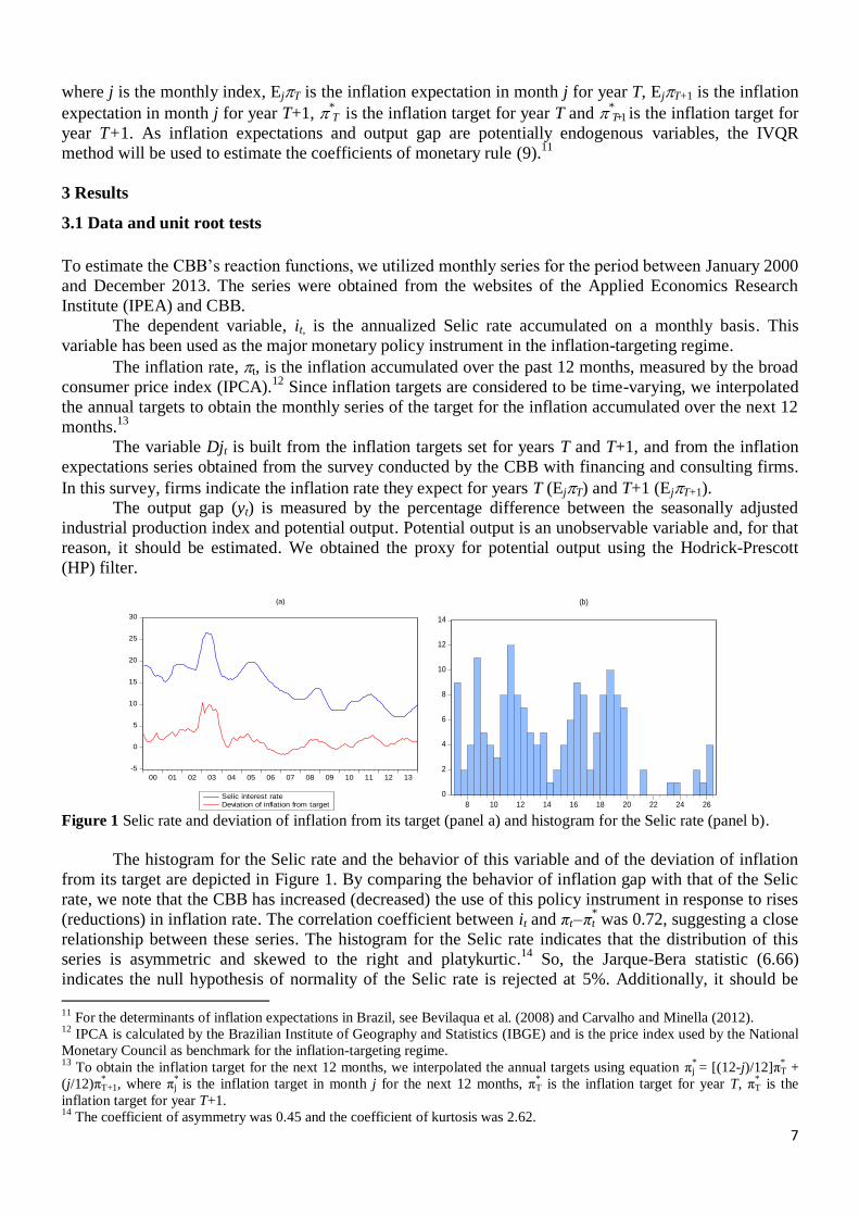
Figure 1 Selic rate and deviation of inflation from its target (panel a) and histogram for the Selic rate (panel b).

The histogram for the Selic rate and the behavior of this variable and of the deviation of inflation

from its target are depicted in Figure 1. By comparing the behavior of inflation gap with that of the Selic

rate, we note that the CBB has increased (decreased) the use of this policy instrument in response to rises

(reductions) in inflation rate. The correlation coefficient between it and πt – π*t was 0.72, suggesting a close

relationship between these series. The histogram for the Selic rate indicates that the distribution of this

series is asymmetric and skewed to the right and platykurtic.14

So, the Jarque-Bera statistic (6.66)

indicates the null hypothesis of normality of the Selic rate is rejected at 5%. Additionally, it should be

11

For the determinants of inflation expectations in Brazil, see Bevilaqua et al. (2008) and Carvalho and Minella (2012). 12

IPCA is calculated by the Brazilian Institute of Geography and Statistics (IBGE) and is the price index used by the National

Monetary Council as benchmark for the inflation-targeting regime. 13

To obtain the inflation target for the next 12 months, we interpolated the annual targets using equation π*j = [(12-j)/12]π

*T +

(j/12)π*T+1, where π

*j is the inflation target in month j for the next 12 months, π

*T is the inflation target for year T, π

*T is the

inflation target for year T+1. 14

The coefficient of asymmetry was 0.45 and the coefficient of kurtosis was 2.62.

8

noted that the Selic rate is way above zero at the lower quantiles. This suggests that the fear of a lower

bound with value zero cannot explain possible asymmetric reactions of the CBB in the lower tail of the

conditional distribution of it.

Before resuming the estimations, we checked whether the variables used in this study are

stationary. Initially, we investigated the order of integration of the variables by the application of three

tests: ADF (Augmented Dickey-Fuller), and MZαGLS

and MZtGLS

tests, suggested by Perron and Ng (1996)

and Ng and Perron (2001).15

As pointed out by Ng and Perron (2001), the selection of the number of lags

(k) was based on the modified Akaike information criterion (MAIC) regarded as the maximum number of

lags of kmax = int(12(T/100)1/4

) = 13. Constant (c) and a linear trend (t) were included as deterministic

components for the cases in which these components were statistically significant.

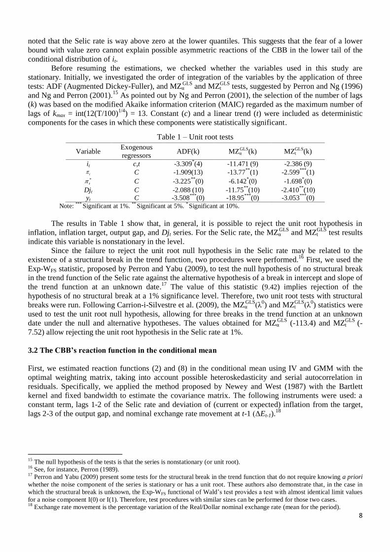
Table 1 – Unit root tests

Variable Exogenous

regressors ADF(k) MZα

GLS(k) MZt

GLS(k)

it c,t -3.309*(4)

-11.471 (9) -2.386 (9)

t C -1.909(13) -13.77**

(1) -2.599***

(1) *

t C -3.225**

(0) -6.142*(0) -1.698

*(0)

Djt C -2.088 (10) -11.75**

(10) -2.410**

(10) yt C -3.508

***(0)

-18.95

***(0) -3.053

***(0)

Note: ***

Significant at 1%. **

Significant at 5%. * Significant at 10%.

The results in Table 1 show that, in general, it is possible to reject the unit root hypothesis in

inflation, inflation target, output gap, and Djt series. For the Selic rate, the MZαGLS

and MZtGLS

test results

indicate this variable is nonstationary in the level.

Since the failure to reject the unit root null hypothesis in the Selic rate may be related to the

existence of a structural break in the trend function, two procedures were performed.16

First, we used the

Exp-WFS statistic, proposed by Perron and Yabu (2009), to test the null hypothesis of no structural break

in the trend function of the Selic rate against the alternative hypothesis of a break in intercept and slope of

the trend function at an unknown date.17

The value of this statistic (9.42) implies rejection of the

hypothesis of no structural break at a 1% significance level. Therefore, two unit root tests with structural

breaks were run. Following Carrion-i-Silvestre et al. (2009), the MZαGLS

(λ0) and MZt

GLS(λ

0) statistics were

used to test the unit root null hypothesis, allowing for three breaks in the trend function at an unknown

date under the null and alternative hypotheses. The values obtained for MZαGLS

(-113.4) and MZtGLS

(-

7.52) allow rejecting the unit root hypothesis in the Selic rate at 1%.

3.2 The CBB’s reaction function in the conditional mean

First, we estimated reaction functions (2) and (8) in the conditional mean using IV and GMM with the

optimal weighting matrix, taking into account possible heteroskedasticity and serial autocorrelation in

residuals. Specifically, we applied the method proposed by Newey and West (1987) with the Bartlett

kernel and fixed bandwidth to estimate the covariance matrix. The following instruments were used: a

constant term, lags 1-2 of the Selic rate and deviation of (current or expected) inflation from the target,

lags 2-3 of the output gap, and nominal exchange rate movement at t-1 (ΔEt-1).18

15

The null hypothesis of the tests is that the series is nonstationary (or unit root). 16

See, for instance, Perron (1989). 17

Perron and Yabu (2009) present some tests for the structural break in the trend function that do not require knowing a priori

whether the noise component of the series is stationary or has a unit root. These authors also demonstrate that, in the case in

which the structural break is unknown, the Exp-WFS functional of Wald’s test provides a test with almost identical limit values

for a noise component I(0) or I(1). Therefore, test procedures with similar sizes can be performed for those two cases. 18

Exchange rate movement is the percentage variation of the Real/Dollar nominal exchange rate (mean for the period).

9

Table 2 – Estimates of the CBB’s reaction functions Parameters Eqn. (2) Eqn. (8)

IV GMM IV GMM

β′0 0.179***

(0.067) 0.171

***

(0.061) 0.120

(0.088) 0.134

*

(0.076)

β′1 0.025

(0.017) 0.016

(0.014) 0.115

***

(0.029) 0.111

***

(0.030)

β′2 0.037***

(0.009)

0.039***

(0.008)

0.042***

(0.010)

0.043***

(0.010) θ1 1.753

***

(0.062)

1.716***

(0.058)

1.627***

(0.068)

1.627***

(0.063) θ2 -0.770

***

(0.062) -0.732

***

(0.057) -0.644

***

(0.070) -0.645

***

(0.063)

β1 1.452 (1.005)

0.995

(0.798) 7.067

**

(3.104) 6.377

***

(2.190) β2 2.196

***

(0.771)

2.407***

(0.865)

2.602**

(1.125)

2.469***

(0.931) J-statistic (p-value) 0.213 0.486 0.803 0.664

Hausman test (p-value) 0.008 0.036 0.000 0.017 Cragg-Donald F-stat 26.61

† 26.61

† 24.00

† 24.00

†

R2-adjusted 0.996 0.996 0.996 0.996

Note: ***

Significant at 1%. **

Significant at 5%. * Significant at 10%. Standard deviation (in brackets).

† Indicates that the

relative bias of the IV (or GMM) in relation to the OLS estimator corresponds to at most 5%.

The set of instruments implies three overidentification constraints. We tested the validity of these

constraints with Hansen’s (1982) J test. Additionally, another two tests were employed: i) Durbin-Wu-

Hausman’ test to verify the null hypothesis of exogeneity of regressors πt – π*t and yt in equation (2), and

Djt and yt in equation (8); and ii) Cragg-Donald’s F test, proposed by Stock and Yogo (2005), to test the

null hypothesis that the instruments are weak.19,20

The results of these tests, shown in Table 2, indicate we

may reject the hypotheses that (current or expected) inflation gap and output gap are exogenous and that

the instruments used in the regressions are weak. Also, the J test shows we cannot reject the hypothesis

that the overidentification constraints are met.

The estimates of the CBB’s reaction function parameters obtained by IV and GMM are quite

similar. For specification (2), the values of the coefficients that measure short-term (β′1 ) and long-term (β1)

responses of the Selic rate to inflation were not statistically different from zero in the conditional interest

rate mean. This suggests that the CBB has not adopted a stabilization policy for the current inflation

around the inflation target, as the increase in inflation has not been followed by a significant increase in

the Selic rate. On the other hand, the Selic rate responded to the changes in output gap. The long-term

coefficients of this variable were equal to 2.2 and 2.4 for rule (2) estimated by IV and GMM,

respectively, and were significant at 1%. Finally, the Selic rate smoothing (θ1+θ2) yielded approximately

0.98. This result is consistent with the literature on short-term interest rate smoothing and indicates the

adjustment of this policy instrument at discrete intervals and in discrete amounts.21

With respect to monetary rule (8), the estimates of coefficient β1 indicate that, in the conditional

Selic rate mean, the CBB has reacted strongly to the deviation of expected inflation from the inflation

target. Specifically, the values obtained for this parameter show the monetary policy rule fulfills the

Taylor principle (1993), i.e., the CBB has increased the Selic rate just enough to rise the real interest rate in response to an increase in expected inflation. This result is in line with those encountered by Minella et

al. (2003), Moura and Carvalho (2010), Sanches-Fung (2011), Aragón and Medeiros (2013) and Minella

and Souza-Sobrinho (2013). Compared to the estimates of β1 for reaction function (2), the CBB has

19

As underscored by Stock and Yogo (2005), the presence of weak instruments may yield biased IV estimators. Thus,

following these authors, we considered instruments to be weak when the bias of the IV or GMM estimator relative to the bias

of the OLS estimator was greater than any value b (for example, b = 5%). 20 The critical values of this test are described in Stock andYogo (2005). 21

For short-term interest rate smoothing, see Goodfriend (1991) and Rudebusch (1995).

10

responded more strongly to expected inflation than to current inflation. This procedure is consistent with

a forward-looking policy rule and indicates the CBB has been concerned mainly with anchoring inflation

expectations to the inflation target set by the National Monetary Council. In regard to coefficient β2, the

results were analogous to those obtained for monetary rule (2) and show the Brazilian monetary authority

has also reacted to the demand pressure.

3.3 Quantile regression results

Now, we present the results for the CBB’s reaction function estimated by IVQR. Figure 2 contains the

coefficients estimated by quantile regressions and the 90% confidence bands. The estimates for each

quantile τ ϵ {0.05,0.1, 0.2,...,0.9, 0.95} are shown. Unlike IV and GMM results, the short-term Selic

interest rate response to inflation gap, β′1 (τ), is statistically different from zero from quantile 0.5 to

quantile 0.9. In contrast, the response to inflation is not significant for the lower quantiles of the

conditional Selic rate distribution. Hence, results reveal that the CBB’s response to inflation gap is

stronger when the Selic rate is adjusted to a higher level than its conditional median. In addition, the

response to inflation is more intense between quantiles 0.5 and 0.9. This result is also observed by

Chevapatrakul et al. (2009) and Wolters (2012) for the Federal Reserve, and by Chevapatrakul and Paez-

Farrell (2014) for the Central Bank of Australia.

Figure 2 also shows that the short-term response of the Selic rate to output gap is significant from

quantile 0.1 to quantile 0.8 and is not statistically different from zero at the extreme quantiles of the

conditional interest rate distribution. In comparison with the IV results, the response to the output gap in

the conditional mean is, in general, stronger than the estimates obtained for the quantiles. However, this

difference is subtle as the confidence interval for the IV estimate includes those estimates obtained by

IVQR.

Figure 2 Estimated coefficients od reaction function (4). Notes: Solid lines show IVQR estimates together with

90% confidence bands of 1000 bootstraps. Dashed lines show IV estimates together with 90% confidence bands.

The results regarding the interest rate smoothing coefficients are significantly different from zero.

Between quantiles 0.05 and 0.8, there was a reduction in coefficient θ1(τ), whereas θ2(τ) increased. By

adding up θ1(τ) + θ2(τ), we verify that the Selic rate smoothing went up from 0.959 at quantile 0.05 to

0.981 at quantile 0.95. This demonstrates that the CBB’s monetary policy is characterized by large

smoothing of the Selic rate and that this smoothing increases at the higher quantiles along the distribution.

Figure 3 depicts the long-term responses of the Selic rate to deviations of inflation from the target

and to output gap for specification (4). The solid line shows the coefficients obtained by IVQR and the

dashed lines show the IV estimates with 90% confidence bands. Consonant with Wolters (2012), we do

not provide the confidence interval for the coefficients at the quantiles because, in general, we had high

11

standard errors which, consequently, implied rather broad confidence intervals.22

A possible explanation

for that is that the sum of the smoothing parameters is very close to 1, yielding very high estimates for the

standard errors obtained by the Delta method.23

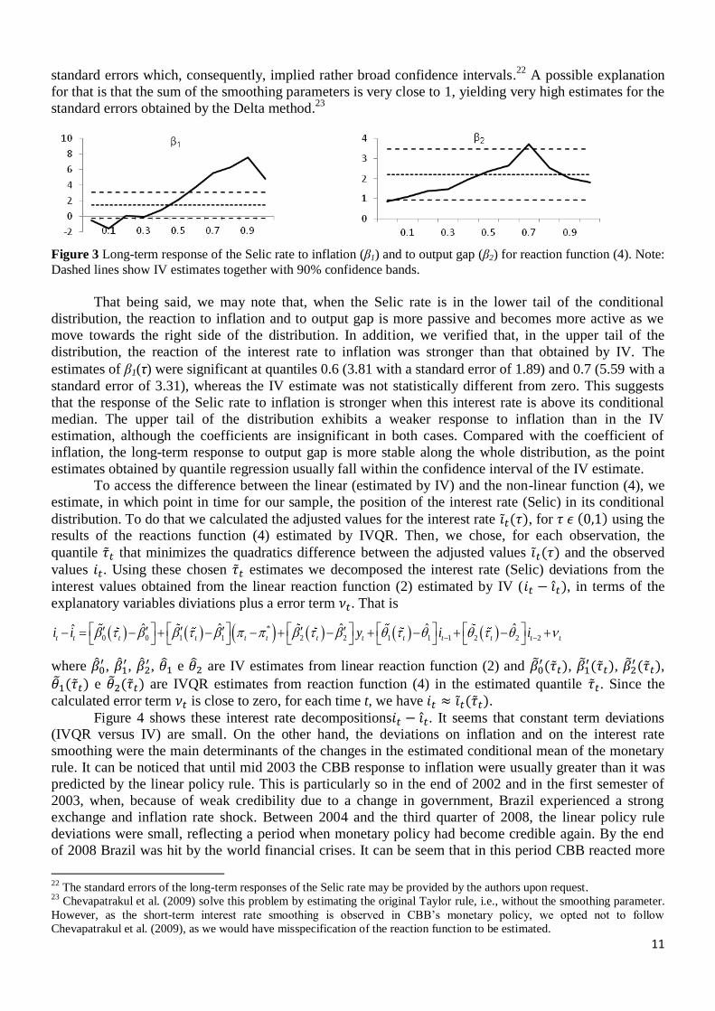
Figure 3 Long-term response of the Selic rate to inflation (β1) and to output gap (β2) for reaction function (4). Note:

Dashed lines show IV estimates together with 90% confidence bands.

That being said, we may note that, when the Selic rate is in the lower tail of the conditional

distribution, the reaction to inflation and to output gap is more passive and becomes more active as we

move towards the right side of the distribution. In addition, we verified that, in the upper tail of the

distribution, the reaction of the interest rate to inflation was stronger than that obtained by IV. The

estimates of β1(τ) were significant at quantiles 0.6 (3.81 with a standard error of 1.89) and 0.7 (5.59 with a

standard error of 3.31), whereas the IV estimate was not statistically different from zero. This suggests

that the response of the Selic rate to inflation is stronger when this interest rate is above its conditional

median. The upper tail of the distribution exhibits a weaker response to inflation than in the IV

estimation, although the coefficients are insignificant in both cases. Compared with the coefficient of

inflation, the long-term response to output gap is more stable along the whole distribution, as the point

estimates obtained by quantile regression usually fall within the confidence interval of the IV estimate.

To access the difference between the linear (estimated by IV) and the non-linear function (4), we

estimate, in which point in time for our sample, the position of the interest rate (Selic) in its conditional

distribution. To do that we calculated the adjusted values for the interest rate , for using the results of the reactions function (4) estimated by IVQR. Then, we chose, for each observation, the

quantile that minimizes the quadratics difference between the adjusted values and the observed

values . Using these chosen estimates we decomposed the interest rate (Selic) deviations from the

interest values obtained from the linear reaction function (2) estimated by IV ( , in terms of the

explanatory variables diviations plus a error term . That is

*

0 0 1 1 2 2 1 1 1 2 2 2ˆ ˆ ˆ ˆ ˆˆ

t t t t t t t t t t t t ti i y i i

where ,

, , e are IV estimates from linear reaction function (2) and

, ,

, e are IVQR estimates from reaction function (4) in the estimated quantile . Since the

calculated error term is close to zero, for each time t, we have .

Figure 4 shows these interest rate decompositions . It seems that constant term deviations (IVQR versus IV) are small. On the other hand, the deviations on inflation and on the interest rate

smoothing were the main determinants of the changes in the estimated conditional mean of the monetary

rule. It can be noticed that until mid 2003 the CBB response to inflation were usually greater than it was

predicted by the linear policy rule. This is particularly so in the end of 2002 and in the first semester of

2003, when, because of weak credibility due to a change in government, Brazil experienced a strong

exchange and inflation rate shock. Between 2004 and the third quarter of 2008, the linear policy rule

deviations were small, reflecting a period when monetary policy had become credible again. By the end

of 2008 Brazil was hit by the world financial crises. It can be seem that in this period CBB reacted more

22

The standard errors of the long-term responses of the Selic rate may be provided by the authors upon request. 23

Chevapatrakul et al. (2009) solve this problem by estimating the original Taylor rule, i.e., without the smoothing parameter.

However, as the short-term interest rate smoothing is observed in CBB’s monetary policy, we opted not to follow

Chevapatrakul et al. (2009), as we would have misspecification of the reaction function to be estimated.

12

strongly to the output gap than it was predicted by the linear rule. Finally, between 2010 and 2012 the

CBB kept the basic interest rate (Selic) below what would be recommended (predicted) by the conditional

mean policy rule. This happens partially because of negative deviations of the IVQR constant in relation

of the IV constant. This may be a reflecting a setting of the basic interest rate systematically below what

would be recommended by the linear reaction function. The policy response to the inflation gap was also

smaller than it was suggested by the linear reaction function in that same period.

Figure 4 Decomposition of policy deviations from the values implied by policy rule (2) estimated at the

conditional mean. Note: The bars denote differences between estimated policy reactions and policy reactions

implied by a policy rule estimated at the conditional mean (constant:

, inflation:

,

output gap:

, interest rate smoothing: ).

Figure 5 shows the short-term coefficients of monetary rule (9) estimated for the quantiles. The

short-term response of the Selic rate to the expected inflation gap is statistically different from quantile

0.4 onwards. Results also demonstrate that this response has an uptrend as we move towards the right side

of the conditional Selic rate distribution. Moreover, note that from quantile 0.6, the estimate of β′1 (τ) is

higher than the estimate obtained by IV. Nonetheless, this difference is not significant, as the confidence

intervals of the estimates at the quantiles include the point IV estimate. Finally, when we compare these

results with those shown in Figure 2, we verify that the short-term response of the Selic rate to the

expected inflation gap is stronger than that to the current inflation gap between quantiles 0.4 and 0.95.

This indicates that the CBB’s forward-looking behavior is observed not only in the conditional mean, but

also in most of the Selic rate distribution.

Figure 5 Estimated coefficients of reaction function (9). Notes: Solid lines show IVQR estimates together with

90% confidence bands of 1000 bootstraps. Dashed lines show IV estimates together with 90% confidence bands.

The response of output gap is significant between quantiles 0.05 and 0.9 and shows a downtrend

along the conditional interest rate distribution. With respect to interest rate smoothing, it should be noted

that the coefficient θ1(τ) has a downtrend whereas the coefficient θ2(τ) exhibits the opposite behavior. As

with monetary rule (4), the sum θ1(τ) + θ2(τ) indicates larger smoothing at the upper quantiles of the Selic

rate distribution.

-1.5

-1

-0.5

0

0.5

1

2002 2004 2006 2008 2010 2012

interest rate smoothing output inflation constant

13

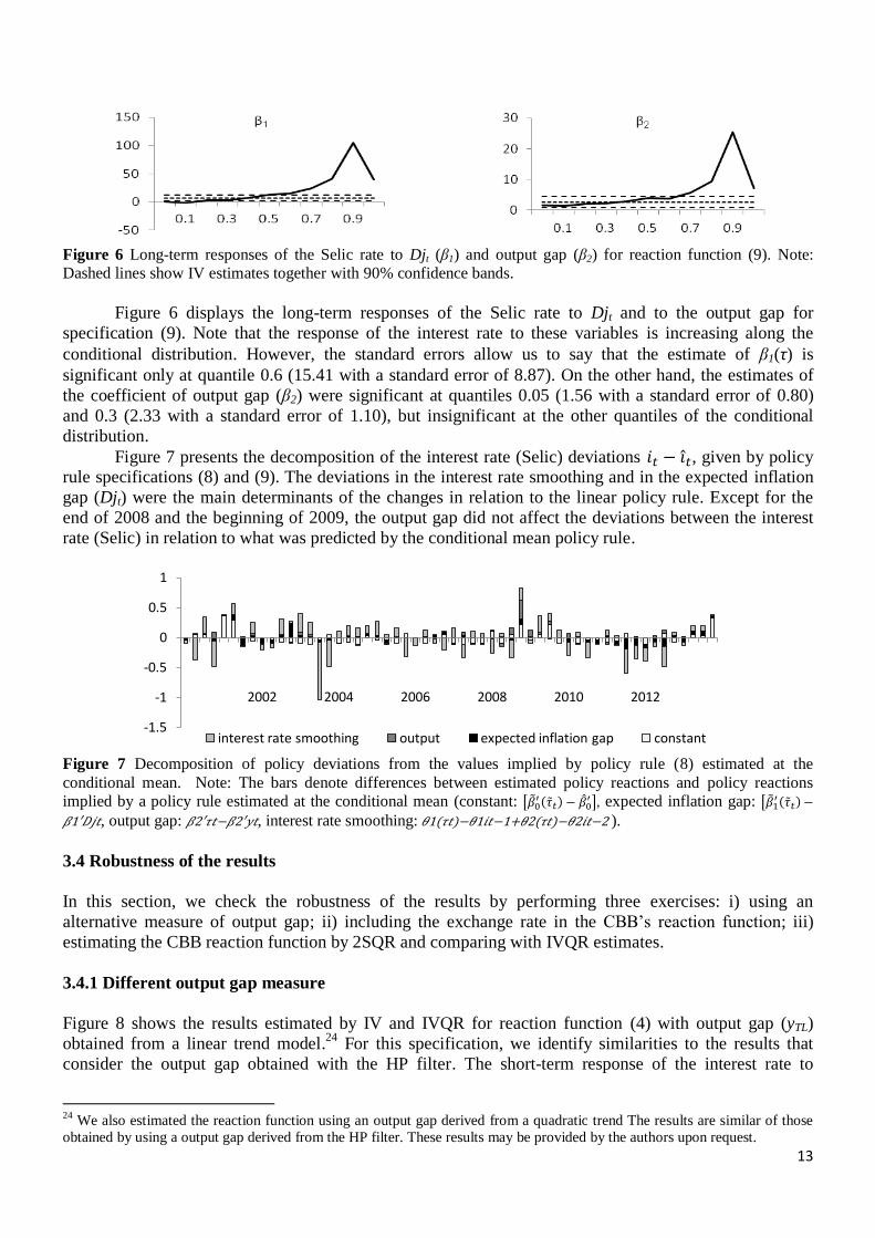
Figure 6 Long-term responses of the Selic rate to Djt (β1) and output gap (β2) for reaction function (9). Note:

Dashed lines show IV estimates together with 90% confidence bands.

Figure 6 displays the long-term responses of the Selic rate to Djt and to the output gap for

specification (9). Note that the response of the interest rate to these variables is increasing along the

conditional distribution. However, the standard errors allow us to say that the estimate of β1(τ) is

significant only at quantile 0.6 (15.41 with a standard error of 8.87). On the other hand, the estimates of

the coefficient of output gap (β2) were significant at quantiles 0.05 (1.56 with a standard error of 0.80)

and 0.3 (2.33 with a standard error of 1.10), but insignificant at the other quantiles of the conditional

distribution.

Figure 7 presents the decomposition of the interest rate (Selic) deviations , given by policy rule specifications (8) and (9). The deviations in the interest rate smoothing and in the expected inflation

gap (Djt) were the main determinants of the changes in relation to the linear policy rule. Except for the

end of 2008 and the beginning of 2009, the output gap did not affect the deviations between the interest

rate (Selic) in relation to what was predicted by the conditional mean policy rule.

Figure 7 Decomposition of policy deviations from the values implied by policy rule (8) estimated at the

conditional mean. Note: The bars denote differences between estimated policy reactions and policy reactions

implied by a policy rule estimated at the conditional mean (constant:

, expected inflation gap:

1′ , output gap: 2′ 2′ , interest rate smoothing: 1( 1 1+ 2( 2 2 ).

3.4 Robustness of the results

In this section, we check the robustness of the results by performing three exercises: i) using an

alternative measure of output gap; ii) including the exchange rate in the CBB’s reaction function; iii)

estimating the CBB reaction function by 2SQR and comparing with IVQR estimates.

3.4.1 Different output gap measure

Figure 8 shows the results estimated by IV and IVQR for reaction function (4) with output gap (yTL)

obtained from a linear trend model.24

For this specification, we identify similarities to the results that

consider the output gap obtained with the HP filter. The short-term response of the interest rate to

24

We also estimated the reaction function using an output gap derived from a quadratic trend The results are similar of those

obtained by using a output gap derived from the HP filter. These results may be provided by the authors upon request.

-1.5

-1

-0.5

0

0.5

1

2002 2004 2006 2008 2010 2012

interest rate smoothing output expected inflation gap constant

14

inflation is increasing along the distribution. In addition, in the upper tail of the conditional distribution,

this response has been stronger than the results estimated by IV and statistically different from zero

between quantiles 0.5 and 0.9. Regarding the short-term response to the output gap, it is significant from

quantile 0.05 to quantile 0.7 and shows an uptrend.

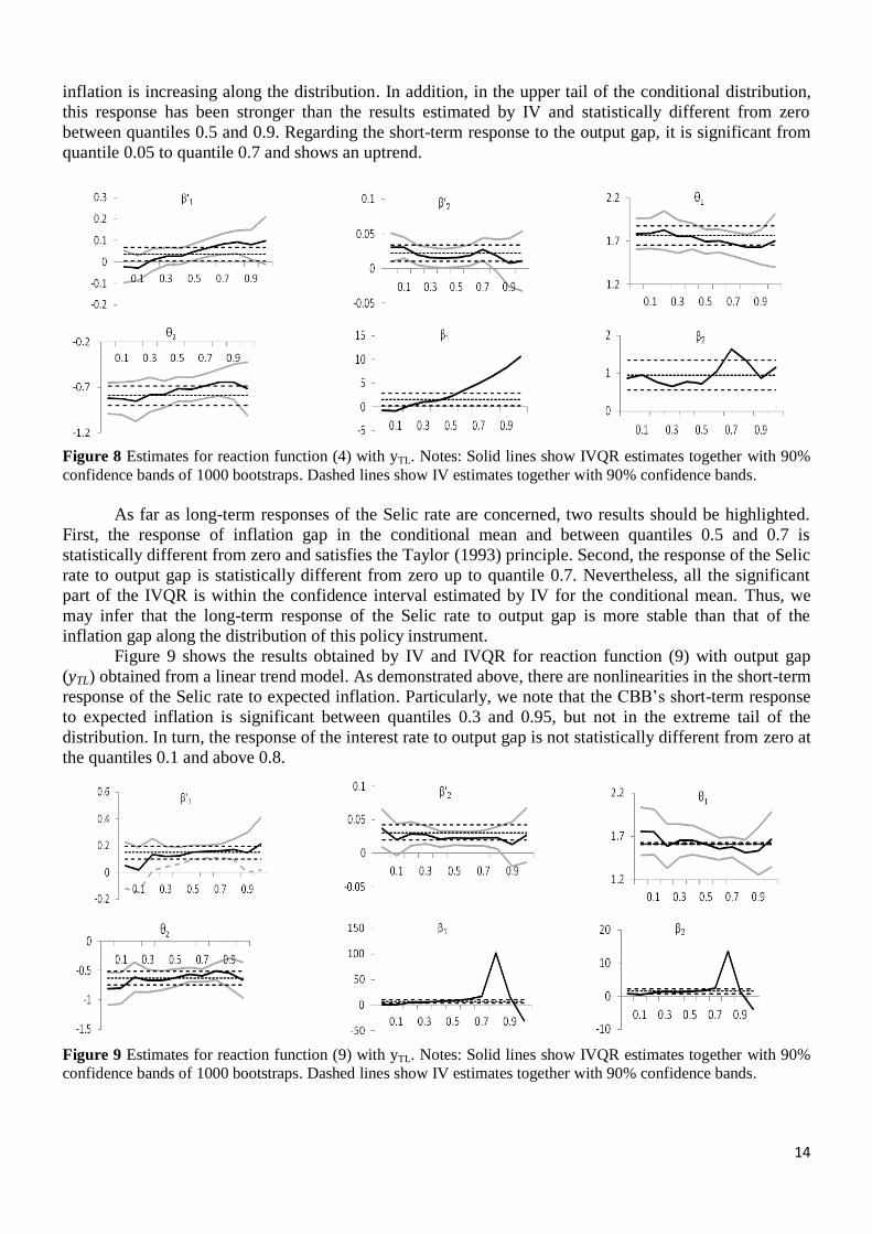
Figure 8 Estimates for reaction function (4) with yTL. Notes: Solid lines show IVQR estimates together with 90%

confidence bands of 1000 bootstraps. Dashed lines show IV estimates together with 90% confidence bands.

As far as long-term responses of the Selic rate are concerned, two results should be highlighted.

First, the response of inflation gap in the conditional mean and between quantiles 0.5 and 0.7 is

statistically different from zero and satisfies the Taylor (1993) principle. Second, the response of the Selic

rate to output gap is statistically different from zero up to quantile 0.7. Nevertheless, all the significant

part of the IVQR is within the confidence interval estimated by IV for the conditional mean. Thus, we

may infer that the long-term response of the Selic rate to output gap is more stable than that of the

inflation gap along the distribution of this policy instrument.

Figure 9 shows the results obtained by IV and IVQR for reaction function (9) with output gap

(yTL) obtained from a linear trend model. As demonstrated above, there are nonlinearities in the short-term

response of the Selic rate to expected inflation. Particularly, we note that the CBB’s short-term response

to expected inflation is significant between quantiles 0.3 and 0.95, but not in the extreme tail of the

distribution. In turn, the response of the interest rate to output gap is not statistically different from zero at

the quantiles 0.1 and above 0.8.

Figure 9 Estimates for reaction function (9) with yTL. Notes: Solid lines show IVQR estimates together with 90%

confidence bands of 1000 bootstraps. Dashed lines show IV estimates together with 90% confidence bands.

15

3.4.2 Exchange rate effects

Several studies have investigated whether central banks react directly to exchange rate movements.

Clarida et al. (1998) revealed that the central banks of Germany and of Japan include the real exchange

rate in their reaction functions, even though the magnitude of the reactions is negligible. Mohanty and

Klau (2004) estimated modified Taylor rules and found that several central banks in emerging countries

(e.g., Brazil and Chile) react to exchange rate movements. Lubik and Schorfheide (2007) estimated a

DSGE model for Australia, New Zealand, Canada, and the United Kingdom and verified that only the

central banks of the first two countries react to exchange rate movements. In line with Lubik and

Schorfheide (2007), Furlani et al. (2010) observed that the CBB does not change the Selic rate in response

to exchange rate movements. Mello and Moccero (2009) revealed that the monetary policy instrument

reacts to exchange rate in Mexico, but not in Brazil, Chile, and Colombia. Aizenman et al. (2011) and

Ostry et al. (2012) demonstrated that the central banks of several emerging markets that adopted the

inflation-targeting regime react to exchange rate movements.

Many are the reasons that may lead the monetary authority to show deep concern for the exchange

rate. First, in an economy with part of the debt denominated in foreign currency, exchange rate

devaluations may increase debt service, hinder the balances of firms and banks, limit credit, expand the

number of bankruptcy filings, and reduce employment and aggregate output. Haussmann et al. (2001) and

Calvo and Reinhart (2002) highlight that the effects on economic agents’ balances has been the major

reason why central banks seek to avoid currency devaluations in the presence of external shocks. On the

other hand, Aghion et al. (2009) developed a theoretical model to show that exchange rate appreciations

may reduce firms’ gains and, consequently, their capacity to take loans and make innovations. This would

negatively affect long-term output growth, with a larger impact on economies with a less developed

financial system. Aizenman et al. (2011) proposed a simple macroeconomic model to assess monetary

policy in a small open economy. They verified that a large weight on exchange rate volatility in the

central bank’s loss function strengthens the reaction of the policy instrument to the exchange rate and

may bring welfare gains. These authors also argue that these gains may be larger in emerging economies

or in those which export commodities, are more vulnerable to shocks on the terms of trade, and have a

poorly developed financial system.

To check whether the CBB has reacted to exchange rate movements, we estimate the following

reaction function on the interest rate conditional mean:

*

0 1 2 3 1 1 2 2( )t t t t t t t ti y e i i (11)

where et is the effective real exchange rate gap (i.e., the deviation of the natural log of the effective real

exchange rate from its trend, estimated by the HP filter).25

In this case, the CBB’s reaction function at

quantile τ can be expressed as:

* *

1 2 0 1 2 3 1 1 2 2| , , , ,t t t t t t t t t t t t tq i y e i i y e i i (12)

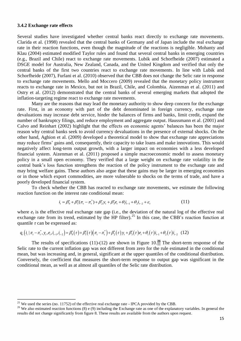
The results of specifications (11)-(12) are shown in Figure 10.26

The short-term response of the

Selic rate to the current inflation gap was not different from zero for the rule estimated in the conditional

mean, but was increasing and, in general, significant at the upper quantiles of the conditional distribution.

Conversely, the coefficient that measures the short-term response to output gap was significant in the

conditional mean, as well as at almost all quantiles of the Selic rate distribution.

25

We used the series (no. 11752) of the effective real exchange rate - IPCA provided by the CBB. 26

We also estimated reaction functions (8) e (9) including the Exchange rate as one of the explanatory variables. In general the

results did not change significantly from figure 8. These results are available from the authors upon request.

16

Figure 10 Estimates for reaction functions (11) and (12). Notes: Solid lines show IVQR estimates together with

90% confidence bands of 1000 bootstraps. Dashed lines show IV estimates together with 90% confidence bands.

Results also reveal that the CBB has a positive response to real exchange rate both in the

conditional mean and along the interest rate distribution. This is consistent with the evidence provided by

Soares and Barbosa (2006), who found a positive response of the Selic rate to real exchange rate, and by

Palma and Portugal (2014), who show that the CBB has given a positive weight to real exchange rate in

its loss function. Finally, results indicate that the response to real exchange rate is usually stronger in the

upper tail of the conditional Selic rate distribution for both specifications.

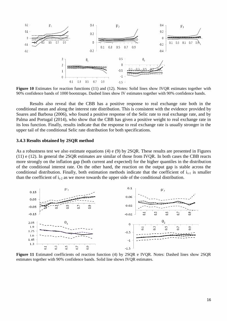
3.4.3 Results obtained by 2SQR method

As a robustness test we also estimate equations (4) e (9) by 2SQR. These results are presented in Figures

(11) e (12). In general the 2SQR estimates are similar of those from IVQR. In both cases the CBB reacts

more strongly on the inflation gap (both current and expected) for the higher quantiles in the distribution

of the conditional interest rate. On the other hand, the reaction on the output gap is stable across the

conditional distribution. Finally, both estimation methods indicate that the coefficient of i t-1 is smaller

than the coefficient of it-2 as we move towards the upper side of the conditional distribution.

Figure 11 Estimated coefficients od reaction function (4) by 2SQR e IVQR. Notes: Dashed lines show 2SQR

estimates together with 90% confidence bands. Solid line shows IVQR estimates.

17

Figure 12 Estimated coefficients od reaction function (9) by 2SQR e IVQR. Notes: Dashed lines show 2SQR

estimates together with 90% confidence bands. Solid line shows IVQR estimates.

4 Conclusions

In this paper, we sought to assess nonlinearities in the CBB’s reaction function by using quantile

regression. As the monetary policy rule has endogenous regressors, we followed the procedures suggested

by Wolters (2012) and the inverse quantile regression (IVQR) method proposed by Chernozhukov and

Hansen (2005, 2006) to estimate the CBB’s quantile reaction function parameters for the inflation-

targeting regime. This method allowed us to detect nonlinearities in the CBB’s reaction function without

having to make specific assumptions about the causal factors that underlie these nonlinearities.

The conditional mean results indicate an insignificant response of the Selic rate to the current

inflation gap, but an otherwise positive one to the deviation of expected inflation from inflation targets.

We also noted that the Selic rate reacted to output gap movements, and the smoothing of this policy

instrument was around 0.98.

The quantile regression results show that the CBB’s short-term response to current inflation was

significant and increasing between quantiles 0.5 and 0.9. In turn, the short-term response of the Selic rate

to output gap increased from quantile 0.2 to quantile 0.7 and was not statistically different from zero at

the extreme quantiles of the conditional interest rate distribution. We also observed that the short-term

response of the Selic rate to the expected inflation gap was significant from quantile 0.4 of the CBB’s

reaction function, exhibiting an uptrend. Concerning the long-term response, results suggest the reactions

of the Selic rate to current and expected inflation were, in general, stronger when the interest rate was

above its median. On the other hand, the long-term response to output gap was significant only at some

quantiles on the interval [0.05, 0.7]. This suggests the CBB does not react to demand pressures when the

interest rate is too high. When we included real exchange rate as a regressor for the interest rate rule, the

CBB had a positive reaction to the real exchange rate both in the conditional mean and along the interest

rate distribution. Moreover, results show the reaction to the real exchange rate was, in general, stronger in

the upper tail of the conditional Selic rate distribution.

References

Adam K, Billi RM (2006) Optimal monetary policy under commitment with a zero bound on nominal

interest rates. J Money Credit Bank 38(7): 1877-1905

Aghion P, Bacchetta, P, Rancière, R, Rogoff, K (2009) Exchange rate volatility and productivity growth:

The role of financial development. J Monetary Econ 56: 494-513

Aizenman J, Hutchison M, Noy I (2011) Inflation Targeting and Real Exchange Rates in Emerging

Markets. World Development 39(5): 712-724

Amemiya T (1982) Two stage least absolute deviations estimators. Econometrica 50: 689-711

18

Aragón EKdaSB, Portugal MS (2010) Nonlinearities in Central Bank of Brazil’s reaction function: the

case of asymmetric preferences. Estudos Econômicos 40(2):373-399

Aragon EKdaSB, Medeiros GB (2013) Testing asymmetries in central bank preferences in a small open

economy: a study for Brazil. EconomiA 14(2): 61-76

Aragon EKdaSB, Medeiros GB (2014) Monetary policy in Brazil: evidence of a reaction function with

time-varying parameters and endogenous regressors. Empir Econ doi: 10.1007/s00181-013-0791-5

Bec F, Salem MB, Collard F (2002) Asymmetries in monetary policy reaction function: evidence for the

U.S., French and German Central Banks. Stud Nonlinear Dyn Econom 6(2):1-22

Bevilaqua AS, Mesquita M, Minella A (2008) Brazil: Taming Inflation Expectation. In: Bank for

International Settlements (ed), Transmission Mechanisms for Monetary Policy in Emerging Market

Economies, BIS Papers 35:139-158

Calvo G, Reinhart C (2002) Fear of floating. Quarterly Journal of Economics 107(2): 379-408.

Carrion-i-Silvestre JL, Kim D, Perron P (2009) GLS-based unit root tests with multiple structural breaks

both under the null and the alternative hypotheses. Econom Theory 25:1754-1792

Carvalho FA, Minella A (2012) Survey forecasts in Brazil: a prismatic assessment of epidemiology,

performance, and determinants. J International Money Finance 31(6):1371-1391

Chen LA, Ponrtnoy S (1996) Two-stage regression quantile and two-stage trimmed least squares

estimators for structural equation models. Commun Stat- Theory Methods 25(5): 1005-1032.

Chevapatrakul, T, Tae-hwan K, Paul M (2009) The Taylor Principle and Monetary Policy Approaching a

Zero Bound on Nominal Rates: Quantile Regression Results for the United States and Japan. J Money

Credit Bank 41(8): 1706-1723

Chevapatrakul T, Paez-farrell J (2014) Monetary Policy reaction Functions in Small Open Economies: a

Quantile Regression Approach. Manch. Sch. 82(2): 237-256

Chernozhukov V, Hansen C (2005) An IV Model of Quantile Treatment Effects. Econometrica 73: 245-

261

Chernozhukov V, Hansen C (2006) Instrumental Quantile Regression Inference for Structural and

Treatment Effect Models. J Econom 132(2): 491-525

Clarida R, Galí J, Gertler M (1998) Monetary policy rules in practice: some international evidence. Eur

Econ Rev 42:1033-1067

Clarida R, Galí J, Gertler M (2000) Monetary policy rules and macroeconomic stability: evidence and

some theory. Q J Econ 115(1):147-180

Cukierman A, Muscatelli V (2008) Non Linear Taylor Rules and Asymmetric Preferences in Central

Banking: evidence from the UK and the US. The B.E J Macroecon 8(1)

de Mello L, Moccero D (2009) Monetary policy and inflation expectations in Latin America: long-run

effects and volatility spillovers. J Money Credit Bank 41:1671-1690

Dolado JJ, Maria-Dolores R, Ruge-Murcia FJ (2004) Nonlinear monetary policy rules: some new

evidence for the US. Stud Nonlinear Dyn Econom 8(3): 1558-3708

Dolado JJ, Maria-Dolores R, Naveira M (2005) Are monetary-policy reaction functions asymmetric? The

role of nonlinearity in the Phillips curve. Eur Econ Rev 49(2): 485-503

Fitzenberger B (1997) The moving blocks bootstrap and robust inference for linear least squares and

quantile regressions. J Econom. 82: 235-287

Furlani LGC, Portugal MS, Laurini, MP (2010) Exchange rate movements and monetary policy in Brazil:

Econometric and simulation evidence. Econ Model 27: 284-295

Goodfriend M. (1991) Interest rates and the conduct of monetary policy. Carnegie–Rochester Series on

Public Policy 34: 7-30

Greene W (2012) Econometric Analysis. 7th edition, Pearson / Prentice Hall

Hansen LP (1982) Large sample properties of generalized method of moments estimators. Econometrica

50(4): 1029-1054

Hausmann R, Ugo P, Ernesto S (2001) Why Do Countries Float the Way They Float? J. Dev Econ 66:

387-414

Kato R, Nishiyama S-I (2005) Optimal monetary policy when interest rates are bounded at zero. J Econ

Dyn Control. 29: 97-133

19

Kim TH, Muller C (2004) Two-Stage Quantile Regression When the First Stage Is based on Quantile

Regression. Econom J 7: 218–231

Kim T-H, Muller C (2012) Bias Transmission and Variance Reduction in Two-Stage Estimation. Aix-

Marseille School of Economics Working Paper No. 1221

Koenker R (2005) Quantile Regression. Econometric Society Monograph, Cambridge University Press,

Cambridge

Koenker R, Bassett G (1978) Regression Quantiles. Econometrica 46(1): 33–50

Koenker R, Hallock K (2001) Quantile Regression: An Introduction. J Econ Perspec 15(2): 143-156

Lopes KC, Aragon EKdaSB (2014) Preferências Assimétricas Variantes no Tempo na Função Perda do

Banco Central do Brasil. Análise Econômica 32(62): 33-62

Lubik TA, Schorfheide F (2007) Do central banks respond to exchange rate movements? A structural

investigation. J Monetary Econ 54: 1069–1087

Minella A, Freitas PS, Goldfajn I, Muinhos MK (2003) Inflation targeting in Brazil: constructing

credibility under exchange rate volatility. J International Money Finance 22(7):1015–1040

Minella A, Souza-Sobrinho NF (2013) Monetary policy in Brazil through the Lens of a Semi-Structural

Model. Econ Model 30:405-419

Mohanty M, Klau M (2004) Monetary policy rules in emerging market economies: issues and evidence.

BIS Working Paper n.149, Basel: Bank for International Settlements

Moura ML, Carvalho Ade (2010) What can Taylor rules say about monetary policy in Latin America? J

Macroecon 32(1):392-404

Newey WK, West KD (1987) A simple, positive semi-definite, heteroskedasticity and autocorrelation

consistent covariance matrix. Econometrica 55(3): 703-708

Ng S, Perron P (2001) Lag length selection and the construction of unit root tests with good size and

power. Econometrica 69(6):1519-1554

Nobay AR, Peel D (2000) Optimal monetary policy with a nonlinear Phillips curve. Econ Lett 67: 159–

164

Nobay AR, Peel DA (2003) Optimal discretionary monetary policy in a model of asymmetric central

bank preferences. Econ J 113: 657-665

Ostry JD, Ghosh, A, Chamon M. (2012) Two Targets, Two Instruments: Monetary and Exchange Rate

Policies in Emerging Market Economies. IMF Staff Discussion Notes, n.12/1

Palma AA, Portugal MS (2014) Preferences of the Central Bank of Brazil under the inflation targeting

regime: estimation using a DSGE model for a small open economy. J Policy Model (fortcoming)

Perron, P (1989) The great crash, the oil price shock and the unit root hypothesis. Econometrica,

57(6):1361-1401

Perron P, Ng S (1996) Useful modifications to some unit root tests with dependent errors and their local

asymptotic properties. Rev Econ Stud 63(3): 435-463

Perron P, Yabu T (2009) Testing for shifts in the trend with an integrated or stationary noise component. J

Bus Econ Stat 27:369-396

Powell J (1983) The asymptotic Normality of Two-Stage Least Absolute Deviations Estimators.

Econometrica 51: 1569-1575

Sá R, Portugal MS (2011) Central bank and asymmetric preferences: an application of sieve estimators to

the U.S. and Brazil, Texto para Discussão, Porto Alegre: PPGE/UFRGS

Sánchez-Fung JR (2011) Estimating monetary policy reaction functions for emerging market economies:

The case of Brazil. Econ Model 28(4):1730-1738

Schaling E (2004) The nonlinear curve and inflation forecast targeting: symmetric versus asymmetric

monetary policy rules. J Money Credit Bank 36(3): 361-386

Schifino, LA, Portugal MS, Tourrucôo F (2013) Regras monetárias ótimas para o Banco Central do

Brasil: considerando a restrição de não negatividade, Texto para Discussão, Porto Alegre: PPGE/UFRGS

Soares JJS, Barbosa FdeH (2006) Regra de Taylor no Brasil: 1999-2005. XXXIV Encontro Nacional de

Economia. Anais. Salvador, 2006.

20

Stock JH, Yogo M (2005) Testing for weak instruments in linear IV regression. In: Identification and

inference for econometric models: Essays in honor of Thomas Rothenberg, ed. D.W. Andrews and J. H.

Stock. Cambridge: Cambridge University Press

Surico P (2007)The Fed's monetary policy rule and U.S. inflation: The case of asymmetric preferences. J.

Econ Dyn Control. 31(1): 305–324

Taylor JB (1993) Discretion versus policy rules in practice. Carnegie-Rochester Conf Ser Public Policy

39:195-214

Tillmann P (2011) Parameter uncertainty and nonlinear monetary policy. Macroecon Dyn 15: 184–200

Wolters MH (2012)Estimating Monetary Policy Reaction Functions Using Quantile Regressions. J

Macroecon 34: 342–361