empirical methods in corporate finance - hbs … methods in corporate finance paul gompers ... 20 25...
TRANSCRIPT

Empirical Methods in Corporate Finance
Paul Gompershb [email protected]
R bi G dRobin [email protected]
Josh Lernerjlerner@hbs [email protected]
Spring 2009Spring 2009
Gompers/Greenwood/Lerner 2009

Good Empirical Research
1. Answers a focused and well specified question
2. Rely on the simplest techniques possible required to establish support for your hypothesis
3. Is well argued and well written
• This course aims to help you with 1 and 2 but mainly 2.
• It takes time to build up the ability to ask good questions, but it is easier when you have an expanded toolkit.
Gompers/Greenwood/Lerner 2009

Administration
• Papers are listed on the syllabus
• We’ll print and bring to class at least one week in advance.
• If you would like to schedule an appointment to meet h f l lwith any of us, please email Peggy
Gompers/Greenwood/Lerner 2009

Course Requirements
• Four referee reports over course of semester
• 5‐15 minute paper proposal and presentation at the end of the semester
• If you audit the course, we hope you still consider doing h l dthe paper proposal and presentation
• While not required, we recommend that you try to replicate some of the main results in papers we cover in class particularly if in a topic that interests youclass, particularly if in a topic that interests you.
Gompers/Greenwood/Lerner 2009

Schedule
Date Topic (s) Instructor
29-Jan Event Studies Robin
5 F b L R bi5-Feb Long-run returns Robin
12-Feb Time-series approaches Robin
19-Feb Panels and Cross-sections 1 Paul
26-Feb Panels and Cross-sections 2 Paul
5-Mar Panels and Cross-sections continued; Combining time-series and cross-section
Paul/Robin
12-Mar Clinical Research (1/2); Experiments and Surveys (1/2);
Josh
19-Mar Experiments and Surveys (1/2); Valuation (1/2); Josh
2-Apr "Structural" Corporate Finance Paul/Robin
9-Apr Using accounting data (1/2); data (1/2) Josh
16-Apr Data Josh/Robin
23-Apr Miscellaneous Paul
30-Apr Presentations: All faculty present
Gompers/Greenwood/Lerner 2009

Advice on Empirical Workf bl• Get a WRDS account if possible
• Even if you work in Stata, you should learn basic SAS for downloading datasets and extracting relevant subsets.g g– Everyone should know basic SQL statements for database work– Key code– SET OPTIONS obs=399999;– This way your programs don’t run forever and you can debugy y p g y g
• Many of the papers on the syllabus have results that are easily replicated. This is a good way to build up your toolkit to do work of your owndo work of your own
• Many corporate finance papers use the Compustat database. As Compustat recently changed all of its variable name mappings older papers require some work to replicatemappings, older papers require some work to replicate.
• I recommend getting acquainted with a good text editor. I prefer “Textpad5”
B t d l d t t l t f SAS St t– Be sure to download syntax templates for SAS, Stata
Gompers/Greenwood/Lerner 2009

Other Useful Resources
Gompers/Greenwood/Lerner 2009

Other Useful Resources
Gompers/Greenwood/Lerner 2009

Lecture 1: Event StudiesLecture 1: Event Studies
Empirical Methods in Corporate FinanceEmpirical Methods in Corporate Finance
Robin Greenwood
January 2009
Gompers/Greenwood/Lerner 2009

Event Studies
• “Analysis of whether there was a statistically significant reaction in financial markets to past occurrences of a i t f t th t i h th i d t ff t fi ’given type of event that is hypothesized to affect firms’ market values.”
• Depending on the application can be used as a measure• Depending on the application, can be used as a measure of the information content of an event (under market efficiency assumption), or as evidence of irrationality (ifefficiency assumption), or as evidence of irrationality (if no news, or statistically significant drift post‐announcement).
• Many famous results in finance derived from event studies…
Gompers/Greenwood/Lerner 2009
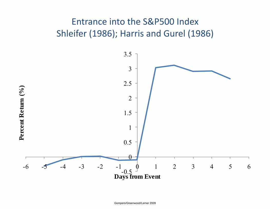
Entrance into the S&P500 IndexShleifer (1986); Harris and Gurel (1986)
3.5
2.5
3
%)
1.5
2
Ret
urn
(%
0.5
1
Perc
ent
0 5
0
0.5
-6 -5 -4 -3 -2 -1 0 1 2 3 4 5 6-0.5
Days from Event
Gompers/Greenwood/Lerner 2009
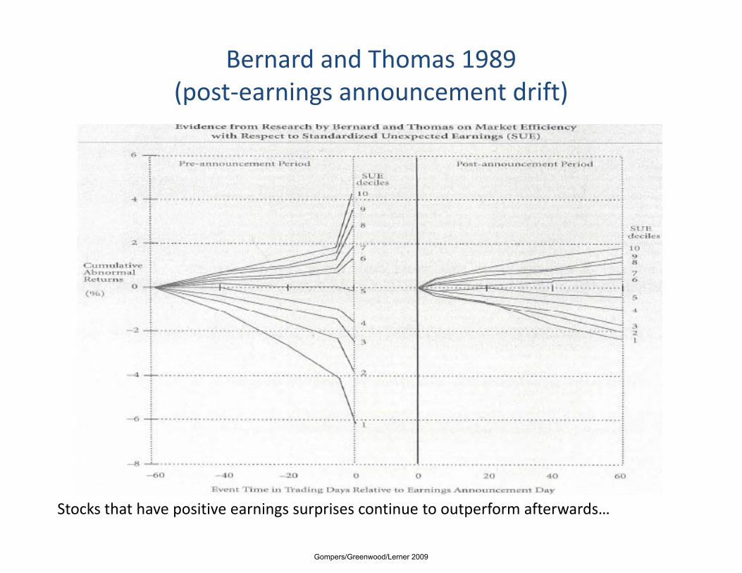
Bernard and Thomas 1989(post‐earnings announcement drift)
Stocks that have positive earnings surprises continue to outperform afterwards…
Gompers/Greenwood/Lerner 2009
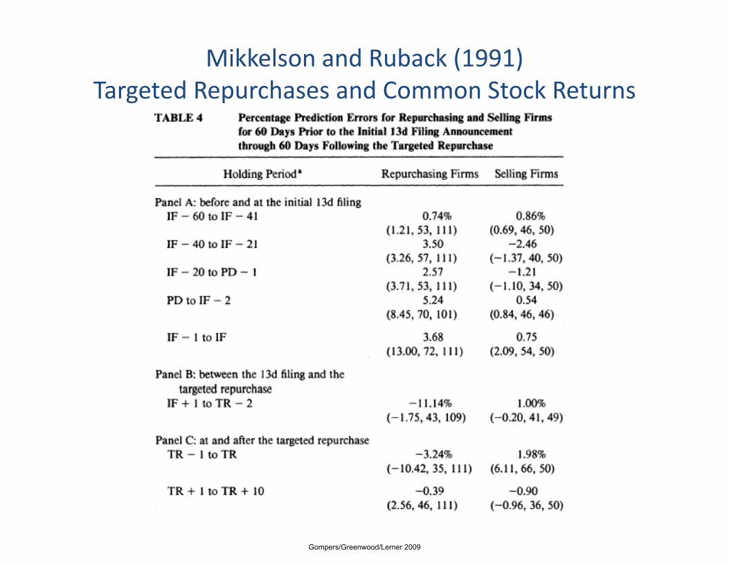
Mikkelson and Ruback (1991)Targeted Repurchases and Common Stock Returns
Gompers/Greenwood/Lerner 2009

Fama, Fisher, Jensen, Roll (1969)Stock Splits
40 Cumulative
3035 abnormal
return %
15
2025
5
1015
05
Month relative to splitp
Gompers/Greenwood/Lerner 2009

Huberman and Regev (2001)
Gompers/Greenwood/Lerner 2009

A rose.com…
Gompers/Greenwood/Lerner 2009

Valuable tool
• If market rationality, impact of news on stock price should allow us to assess impact on firm value of:– Mergers and acquisitions.
– Financing decisions.
Public policy choices– Public policy choices.
• Extensive use in litigation and policy discussions.
Gompers/Greenwood/Lerner 2009
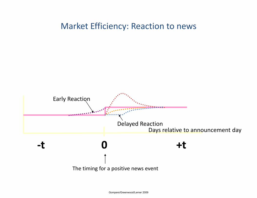
Market Efficiency: Reaction to news
Early Reaction
Days relative to announcement dayDelayed Reaction
00 +t+t‐‐tt
The timing for a positive news event
Gompers/Greenwood/Lerner 2009

Long history…
• First study: Dolley [1933] on stock splits.
• Refinement of technique by late 1960s.
• Formal testing of alternative methods by Brown and Warner [1980, 1985].
• Gradual extension into industrial organization, other economics literature.
Gompers/Greenwood/Lerner 2009

Lecture Plan
• Event Study Design
• Simple example
• Standard significance tests (see CLM, Chapter 4)
• Tips on arranging data for effective use in event studies
• Measures of Abnormal Returns
• Cross‐sectional models– Simple example
• Econometric concerns and more examples– Brown and Warner 1 and 2
– Bittlingmayer and Hazlett
– Greenwood – Returns are correlated for a single event
– Simulating Standard Errors – Barberis, Shleifer and Wurgler
Gompers/Greenwood/Lerner 2009
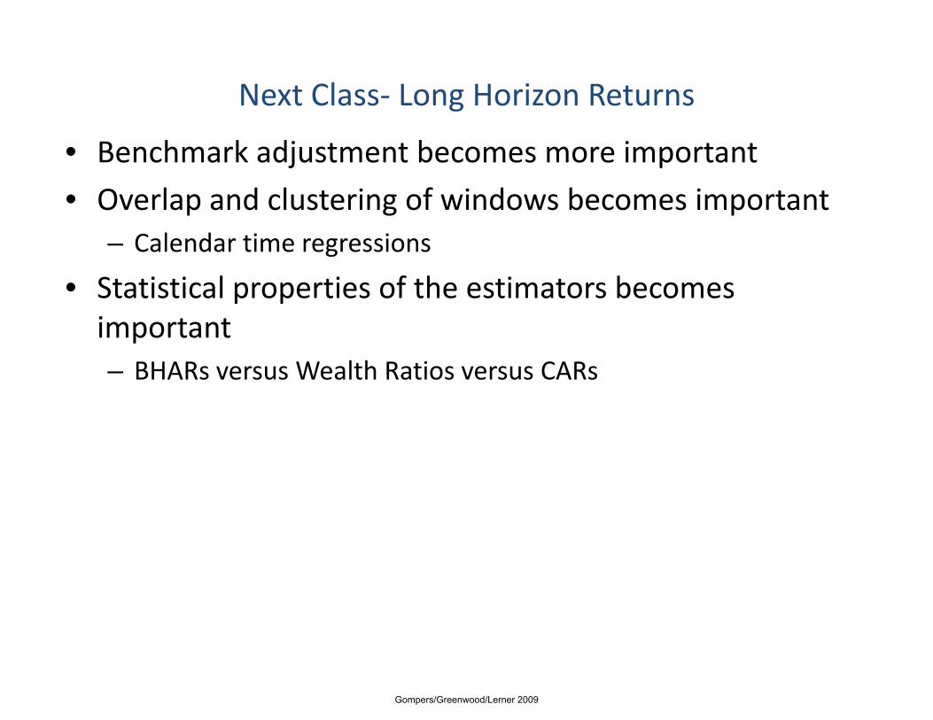
Next Class‐ Long Horizon Returns
• Benchmark adjustment becomes more important
• Overlap and clustering of windows becomes important– Calendar time regressions
• Statistical properties of the estimators becomes important– BHARs versus Wealth Ratios versus CARs
Gompers/Greenwood/Lerner 2009

Crucial elements of any event study
• Event dates.
• Size of “event window”:– Will reflect possibility of leakage, precision of event dating.
• Actual return.
• Expected return.
• Measure of variance.
Gompers/Greenwood/Lerner 2009
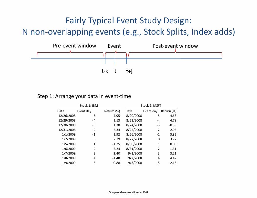
Fairly Typical Event Study Design: N non‐overlapping events (e.g., Stock Splits, Index adds)
Pre‐event window Event Post‐event window
t‐k t t+j
Step 1: Arrange your data in event‐time
Date Event day Return (%) Date Event day Return (%)
Stock 1: IBM Stock 2: MSFT
Date Event day Return (%) Date Event day Return (%)12/26/2008 ‐5 4.95 8/20/2008 ‐5 ‐4.6312/29/2008 ‐4 1.13 8/23/2008 ‐4 4.7812/30/2008 ‐3 1.38 8/24/2008 ‐3 ‐0.3912/31/2008 ‐2 2.34 8/25/2008 ‐2 2.931/1/2009 ‐1 1.92 8/26/2008 ‐1 3.821/2/2009 0 7.79 8/27/2008 0 3.721/5/2009 1 ‐1.75 8/30/2008 1 0.031/6/2009 2 2.24 8/31/2008 2 1.311/7/2009 3 2.40 9/1/2008 3 3.211/8/2009 4 ‐1.48 9/2/2008 4 4.42/ / / /1/9/2009 5 ‐0.88 9/3/2008 5 ‐2.16
Gompers/Greenwood/Lerner 2009

Fairly Typical Event Study Design: N non‐overlapping events (e.g., Stock Splits, Index adds)
Pre‐event window Event Post‐event window
t‐k t t+j
Step 2: Make risk adjustment
Date Event day Return (%) Date Event day Return (%)12/26/2008 ‐5 4.95 8/20/2008 ‐5 ‐4.6312/29/2008 ‐4 1.13 8/23/2008 ‐4 4.7812/30/2008 ‐3 1.38 8/24/2008 ‐3 ‐0.39
Stock 1: IBM Stock 2: MSFT
Date Event day Return (%) Date Event day Return (%)12/26/2008 ‐5 2.67 8/20/2008 ‐5 4.6012/29/2008 ‐4 1.11 8/23/2008 ‐4 13.0112/30/2008 ‐3 3.18 8/24/2008 ‐3 3.26
Stock 1: IBM Stock 2: MSFT
12/30/2008 3 1.38 8/24/2008 3 0.3912/31/2008 ‐2 2.34 8/25/2008 ‐2 2.931/1/2009 ‐1 1.92 8/26/2008 ‐1 3.821/2/2009 0 7.79 8/27/2008 0 3.721/5/2009 1 ‐1.75 8/30/2008 1 0.031/6/2009 2 2.24 8/31/2008 2 1.311/7/2009 3 2.40 9/1/2008 3 3.21
12/30/2008 3 3.18 8/24/2008 3 3.2612/31/2008 ‐2 11.29 8/25/2008 ‐2 ‐0.011/1/2009 ‐1 ‐5.55 8/26/2008 ‐1 ‐0.411/2/2009 0 10.77 8/27/2008 0 5.551/5/2009 1 ‐10.58 8/30/2008 1 ‐3.431/6/2009 2 1.39 8/31/2008 2 ‐6.621/7/2009 3 ‐4.92 9/1/2008 3 ‐0.82/ / / /
1/8/2009 4 ‐1.48 9/2/2008 4 4.421/9/2009 5 ‐0.88 9/3/2008 5 ‐2.16
/ / / /1/8/2009 4 0.31 9/2/2008 4 ‐2.791/9/2009 5 0.09 9/3/2008 5 ‐4.86
Gompers/Greenwood/Lerner 2009
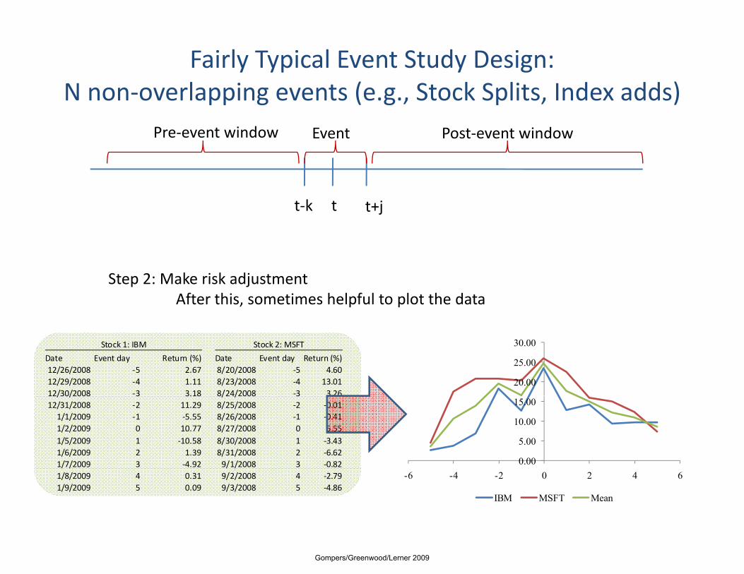
Fairly Typical Event Study Design: N non‐overlapping events (e.g., Stock Splits, Index adds)
Pre‐event window Event Post‐event window
t‐k t t+j
Step 2: Make risk adjustmentAfter this, sometimes helpful to plot the data
20.00
25.00
30.00Date Event day Return (%) Date Event day Return (%)12/26/2008 ‐5 2.67 8/20/2008 ‐5 4.6012/29/2008 ‐4 1.11 8/23/2008 ‐4 13.0112/30/2008 ‐3 3.18 8/24/2008 ‐3 3.26
Stock 1: IBM Stock 2: MSFT
0.00
5.00
10.00
15.0012/30/2008 3 3.18 8/24/2008 3 3.2612/31/2008 ‐2 11.29 8/25/2008 ‐2 ‐0.011/1/2009 ‐1 ‐5.55 8/26/2008 ‐1 ‐0.411/2/2009 0 10.77 8/27/2008 0 5.551/5/2009 1 ‐10.58 8/30/2008 1 ‐3.431/6/2009 2 1.39 8/31/2008 2 ‐6.621/7/2009 3 ‐4.92 9/1/2008 3 ‐0.82
-6 -4 -2 0 2 4 6
IBM MSFT Mean
/ / / /1/8/2009 4 0.31 9/2/2008 4 ‐2.791/9/2009 5 0.09 9/3/2008 5 ‐4.86
Gompers/Greenwood/Lerner 2009

Fairly Typical Event Study Design: N non‐overlapping events (e.g., Stock Splits, Index adds)
Pre‐event window Event Post‐event window
t‐k t t+j
Step 3: Cumulate over desired window
Stock 1: IBM Stock 2: MSFT
Date Event day Return (%) Date Event day Return (%)12/26/2008 ‐5 2.67 8/20/2008 ‐5 4.6012/29/2008 ‐4 1.11 8/23/2008 ‐4 13.0112/30/2008 ‐3 3.18 8/24/2008 ‐3 3.2612/31/2008 ‐2 11.29 8/25/2008 ‐2 ‐0.011/1/2009 ‐1 ‐5 55 8/26/2008 ‐1 ‐0 41
Stock 1: IBM Stock 2: MSFT
Stock 1: IBM Stock 2: MSFT
1/1/2009 1 5.55 8/26/2008 1 0.411/2/2009 0 10.77 8/27/2008 0 5.551/5/2009 1 ‐10.58 8/30/2008 1 ‐3.431/6/2009 2 1.39 8/31/2008 2 ‐6.621/7/2009 3 ‐4.92 9/1/2008 3 ‐0.821/8/2009 4 0.31 9/2/2008 4 ‐2.791/9/2009 5 0.09 9/3/2008 5 ‐4.86
CAR [‐1,0] 5.22 5.14
/ / / /
Gompers/Greenwood/Lerner 2009

Fairly Typical Event Study Design: N non‐overlapping events (e.g., Stock Splits, Index adds)
Pre‐event window Event Post‐event window
t‐k t t+j
Step 4: Can test for significance of Average CAR, or individual CARs
Stock 1: IBM Stock 2: MSFT
Date Event day Return (%) Date Event day Return (%)12/26/2008 ‐5 2.67 8/20/2008 ‐5 4.6012/29/2008 ‐4 1.11 8/23/2008 ‐4 13.0112/30/2008 ‐3 3.18 8/24/2008 ‐3 3.2612/31/2008 ‐2 11.29 8/25/2008 ‐2 ‐0.011/1/2009 ‐1 ‐5 55 8/26/2008 ‐1 ‐0 41
Stock 1: IBM Stock 2: MSFT
Stock 1: IBM Stock 2: MSFT
1/1/2009 1 5.55 8/26/2008 1 0.411/2/2009 0 10.77 8/27/2008 0 5.551/5/2009 1 ‐10.58 8/30/2008 1 ‐3.431/6/2009 2 1.39 8/31/2008 2 ‐6.621/7/2009 3 ‐4.92 9/1/2008 3 ‐0.821/8/2009 4 0.31 9/2/2008 4 ‐2.791/9/2009 5 0.09 9/3/2008 5 ‐4.86
CAR [‐1,0] 5.22 5.14
Take Average
/ / / /
5.18%
Gompers/Greenwood/Lerner 2009

Testing for Statistical Significance
Pre‐event window Event Post‐event window
t‐k t t+j
• Objective is to reject the null hypothesis that the average return is zero.
• Reminder:– Power = probability that test will reject a false null hypothesis =
b b l h ll kProbability that it will not make a type II error.
– Test size = Significance Level = Type 1 error = Probability of rejecting a true null hypothesisrejecting a true null hypothesis
Gompers/Greenwood/Lerner 2009
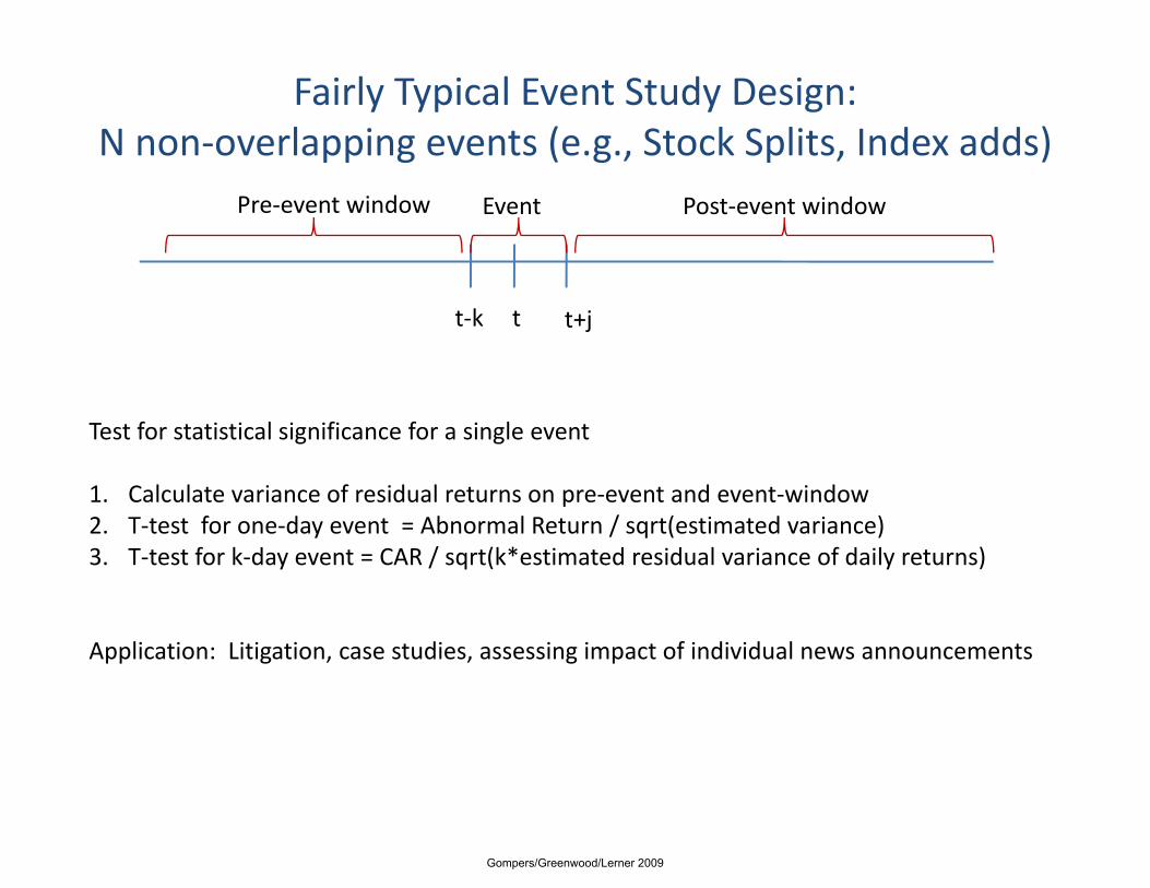
Fairly Typical Event Study Design: N non‐overlapping events (e.g., Stock Splits, Index adds)
Pre‐event window Event Post‐event window
t‐k t t+j
Test for statistical significance for a single event
1. Calculate variance of residual returns on pre‐event and event‐window1. Calculate variance of residual returns on pre event and event window2. T‐test for one‐day event = Abnormal Return / sqrt(estimated variance)3. T‐test for k‐day event = CAR / sqrt(k*estimated residual variance of daily returns)
Application: Litigation, case studies, assessing impact of individual news announcements
Gompers/Greenwood/Lerner 2009

Fairly Typical Event Study Design: N non‐overlapping events (e.g., Stock Splits, Index adds)
Pre‐event window Event Post‐event window
t‐k t t+j
Test for statistical significance for a single event
1. Calculate variance of residual returns on pre‐event and event‐window1. Calculate variance of residual returns on pre event and event window2. T‐test for one‐day event = Abnormal Return / sqrt(estimated variance)3. T‐test for k‐day event = CAR / sqrt(k*estimated residual variance of daily returns)
Related technique: Estimate a regression of R = a + bRm + cEventDummyLess useful for long window events.
Gompers/Greenwood/Lerner 2009

Fairly Typical Event Study Design: N non‐overlapping events (e.g., Stock Splits, Index adds)
Pre‐event window Event Post‐event window
t‐k t t+j
Test for statistical significance for multiple events
1 21
( , )CARt τ τ= 1
2 21 2
2 21 2 1 22 1
ˆ ( , )
1ˆ ˆ( , ) ( , )Nii
t
N
σ τ τ
σ τ τ σ τ τ=
⎡ ⎤⎣ ⎦
= ∑1 2 1 22 1
1 2
( ) ( )
( , )
iiN
N CARt τ τ
=
⇒
⋅=
∑
21 21
ˆ ( , )Nii
tσ τ τ
=∑
Gompers/Greenwood/Lerner 2009
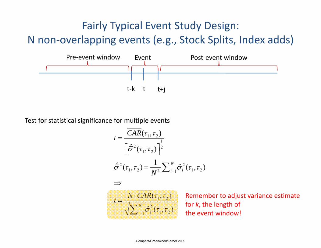
Fairly Typical Event Study Design: N non‐overlapping events (e.g., Stock Splits, Index adds)
Pre‐event window Event Post‐event window
t‐k t t+j
Test for statistical significance for multiple events
1 21
( , )CARt τ τ= 1
2 21 2
2 21 2 1 22 1
ˆ ( , )
1ˆ ˆ( , ) ( , )Nii
t
N
σ τ τ
σ τ τ σ τ τ=
⎡ ⎤⎣ ⎦
= ∑1 2 1 22 1
1 2
( ) ( )
( , )
iiN
N CARt τ τ
=
⇒
⋅=
∑
Remember to adjust variance estimatef k h l h f2
1 21ˆ ( , )N
ii
tσ τ τ
=∑ for k, the length ofthe event window!
Gompers/Greenwood/Lerner 2009

Fairly Typical Event Study Design: N non‐overlapping events (e.g., Stock Splits, Index adds)
Pre‐event window Event Post‐event window
t‐k t t+j
Test for statistical significance for multiple events
1 21
( , )CARt τ τ= Note that this is not the same1
2 21 2
2 21 2 1 22 1
ˆ ( , )
1ˆ ˆ( , ) ( , )Nii
t
N
σ τ τ
σ τ τ σ τ τ=
⎡ ⎤⎣ ⎦
= ∑
Note that this is not the sameAs the cross‐sectional Standard error of the CARsbecause we use pre‐event d t t i f ti t1 2 1 22 1
1 2
( ) ( )
( , )
iiN
N CARt τ τ
=
⇒
⋅=
∑ data to inform our estimate of σ!!!
But cross-sectional standard 2
1 21ˆ ( , )N
ii
tσ τ τ
=∑ error won’t be too far off in most cases.
Gompers/Greenwood/Lerner 2009

Fairly Typical Event Study Design: N non‐overlapping events (e.g., Stock Splits, Index adds)
Pre‐event window Event Post‐event window
t‐k t t+j
Test for statistical significance for multiple events
1 21
( , )CARt τ τ= …And should be exactly the1
2 21 2
2 21 2 1 22 1
ˆ ( , )
1ˆ ˆ( , ) ( , )Nii
t
N
σ τ τ
σ τ τ σ τ τ=
⎡ ⎤⎣ ⎦
= ∑
…And should be exactly the same if the residual standard deviation is the same across securities
1 2 1 22 1
1 2
( ) ( )
( , )
iiN
N CARt τ τ
=
⇒
⋅=
∑
21 21
ˆ ( , )Nii
tσ τ τ
=∑
Gompers/Greenwood/Lerner 2009

Fairly Typical Event Study Design: N non‐overlapping events (e.g., Stock Splits, Index adds)
Pre‐event window Event Post‐event window
t‐k t t+j
Test for statistical significance for multiple events
1 21
( , )CARt τ τ= …One common criticism of1
2 21 2
2 21 2 1 22 1
ˆ ( , )
1ˆ ˆ( , ) ( , )Nii
t
N
σ τ τ
σ τ τ σ τ τ=
⎡ ⎤⎣ ⎦
= ∑
…One common criticism of event studies has been that the variance of returns around the event is higher, in hi h th t t t ill b1 2 1 22 1
1 2
( ) ( )
( , )
iiN
N CARt τ τ
=
⇒
⋅=
∑ which case the t‐stat will be overstated.
Cross‐sectional standard 2
1 21ˆ ( , )N
ii
tσ τ τ
=∑ error partially helps here.
Gompers/Greenwood/Lerner 2009

Fairly Typical Event Study Design: N non‐overlapping events (e.g., Stock Splits, Index adds)
Pre‐event window Event Post‐event window
t‐k t t+j
Cross‐sectional estimator of the variance (Boehmer et al 1991, Page 167 CLM):
( )21[ ( )] ( ) ( )NVar CAR CAR CARτ τ τ τ τ τ= −∑ ( )1 2 1 2 1 22 1[ ( , )] ( , ) ( , )ii
Var CAR CAR CARN
τ τ τ τ τ τ=
= ∑
…Consistent if abnormal returns are uncorrelated in the cross‐sectionCross‐sectional homoskedasticity not required!Cross‐sectional homoskedasticity not required!Benefit of this approach: Very easy to implement, even in Excel !!
Gompers/Greenwood/Lerner 2009

Fairly Typical Event Study Design: N non‐overlapping events (e.g., Stock Splits, Index adds)
Pre‐event window Event Post‐event window
t‐k t t+j
One more technique is to aggregate the individual scaled returns:
ii
CARSCARσ
=
1/2
12
2
( 4) ~ (0,1).4
i
iN LJ SCAR N
L
σ
⎛ ⎞−= ⎜ ⎟−⎝ ⎠⎝ ⎠
…CLM 4.4.24Relevant if CAR variance is higher for high CAR eventsIn practice, I don’t see this very often, stick with simpler method
Gompers/Greenwood/Lerner 2009

Coding tips for doing event studies
• SAS– Steps to compute event‐time
• Start with panel‐>Merge event dates‐>Compute Event timeStart with panel >Merge event dates >Compute Event time• Transpose data in event time and dump to STATA for easy use
• Matlab– Arrange your data in an event‐time matrix
• Stata/Eventus– Eventus can produce a file that already identifies your returns inEventus can produce a file that already identifies your returns in
event time
• ExcelS i bl l f di i h ll l d f i k– Suitable only for studies with small samples and for getting to know your data
• WARNINGS– Watch out for events with duplicate stocks (ie, acquirer buys twice)
Gompers/Greenwood/Lerner 2009
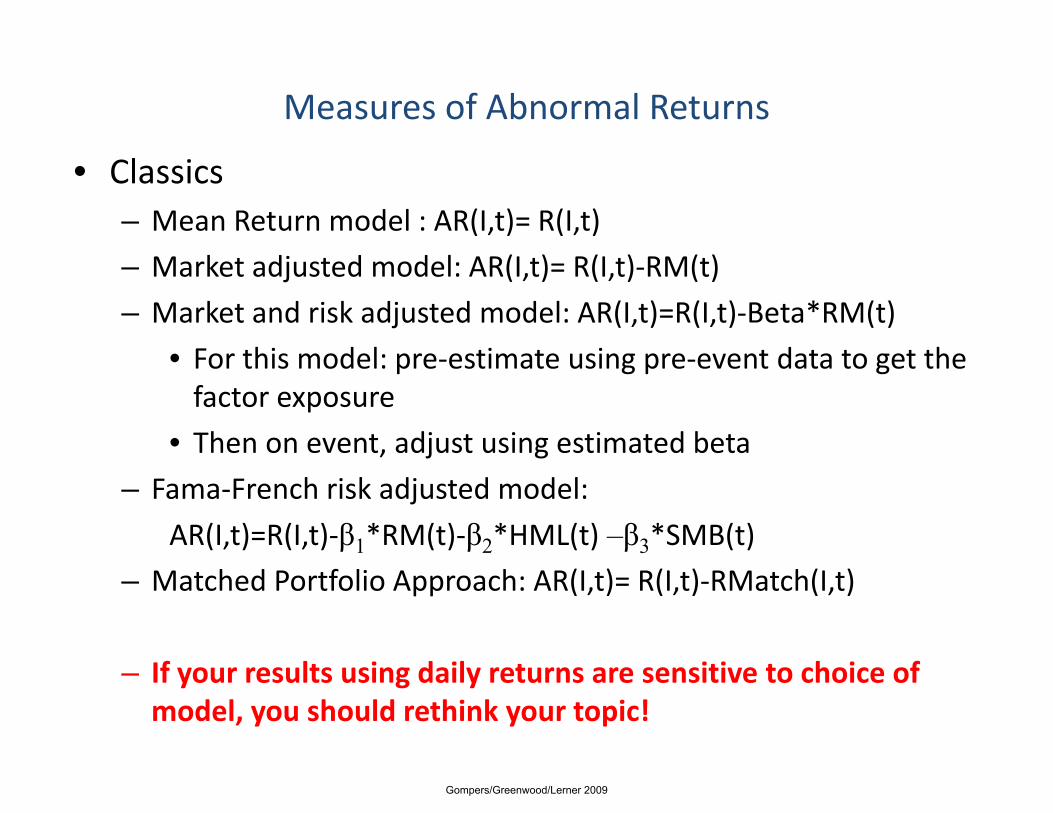
Measures of Abnormal Returns
• Classics– Mean Return model : AR(I,t)= R(I,t)
– Market adjusted model: AR(I,t)= R(I,t)‐RM(t)
– Market and risk adjusted model: AR(I,t)=R(I,t)‐Beta*RM(t)
• For this model: pre estimate using pre event data to get the• For this model: pre‐estimate using pre‐event data to get the factor exposure
• Then on event, adjust using estimated betaj g
– Fama‐French risk adjusted model:
AR(I,t)=R(I,t)‐β1*RM(t)‐β2*HML(t) –β3*SMB(t)
– Matched Portfolio Approach: AR(I,t)= R(I,t)‐RMatch(I,t)
If l i d il i i h i f– If your results using daily returns are sensitive to choice of model, you should rethink your topic!
Gompers/Greenwood/Lerner 2009
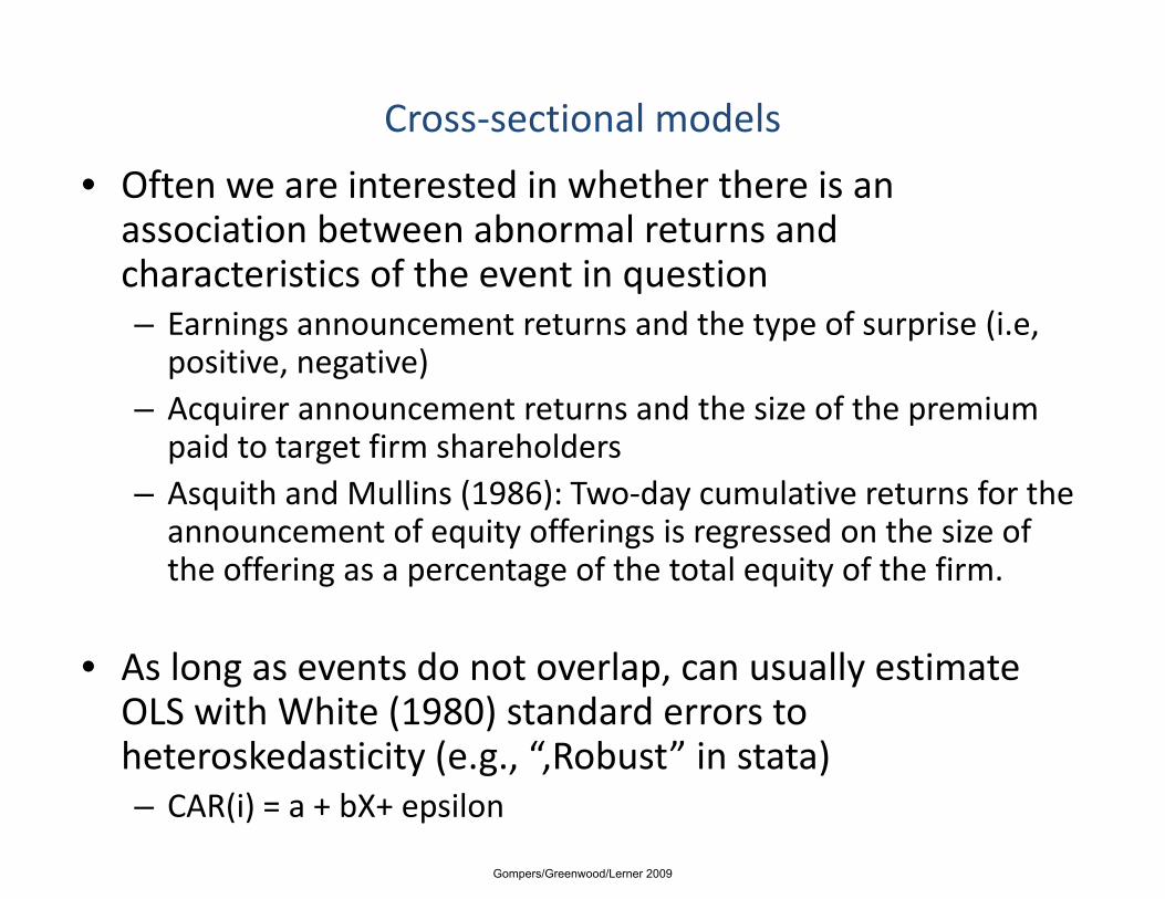
Cross‐sectional models
• Often we are interested in whether there is an association between abnormal returns and characteristics of the event in questioncharacteristics of the event in question– Earnings announcement returns and the type of surprise (i.e, positive, negative)
– Acquirer announcement returns and the size of the premium paid to target firm shareholders
– Asquith and Mullins (1986): Two‐day cumulative returns for the q ( ) yannouncement of equity offerings is regressed on the size of the offering as a percentage of the total equity of the firm.
• As long as events do not overlap, can usually estimate OLS with White (1980) standard errors to heteroskedasticity (e.g., “,Robust” in stata)– CAR(i) = a + bX+ epsilon
Gompers/Greenwood/Lerner 2009
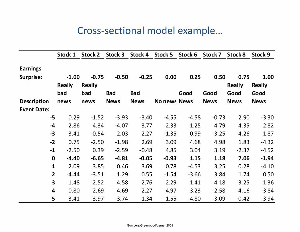
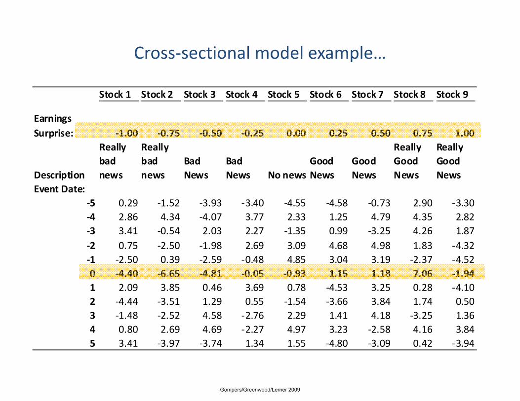
Cross‐sectional model example…
Stock 1 Stock 2 Stock 3 Stock 4 Stock 5 Stock 6 Stock 7 Stock 8 Stock 9
Earnings Surprise: ‐1.00 ‐0.75 ‐0.50 ‐0.25 0.00 0.25 0.50 0.75 1.00
Description
Really bad news
Really bad news
Bad News
Bad News No news
Good News
Good News
Really Good News
Really Good NewsDescription news news News News No news News News News News
Event Date:‐5 0.29 ‐1.52 ‐3.93 ‐3.40 ‐4.55 ‐4.58 ‐0.73 2.90 ‐3.30‐4 2.86 4.34 ‐4.07 3.77 2.33 1.25 4.79 4.35 2.82‐3 3.41 ‐0.54 2.03 2.27 ‐1.35 0.99 ‐3.25 4.26 1.87‐2 0.75 ‐2.50 ‐1.98 2.69 3.09 4.68 4.98 1.83 ‐4.32‐1 ‐2.50 0.39 ‐2.59 ‐0.48 4.85 3.04 3.19 ‐2.37 ‐4.520 ‐4.40 ‐6.65 ‐4.81 ‐0.05 ‐0.93 1.15 1.18 7.06 ‐1.940 4.40 6.65 4.81 0.05 0.93 1.15 1.18 7.06 1.941 2.09 3.85 0.46 3.69 0.78 ‐4.53 3.25 0.28 ‐4.102 ‐4.44 ‐3.51 1.29 0.55 ‐1.54 ‐3.66 3.84 1.74 0.503 ‐1.48 ‐2.52 4.58 ‐2.76 2.29 1.41 4.18 ‐3.25 1.364 0 80 2 69 4 69 2 27 4 97 3 23 2 58 4 16 3 844 0.80 2.69 4.69 ‐2.27 4.97 3.23 ‐2.58 4.16 3.845 3.41 ‐3.97 ‐3.74 1.34 1.55 ‐4.80 ‐3.09 0.42 ‐3.94
Gompers/Greenwood/Lerner 2009

Plot the data
8.00
4.00
6.00
0.00
2.00
1 50 1 00 0 50 0 00 0 50 1 00 1 50urns
-4.00
-2.00-1.50 -1.00 -0.50 0.00 0.50 1.00 1.50
Ret
u
-8.00
-6.00
Earnings Surprise
Gompers/Greenwood/Lerner 2009

Estimate Regression
R = 4.28 EARNSURPRISE - 1.046.00
8.00
0 00
2.00
4.00
s
4 00
-2.00
0.00-1.50 -1.00 -0.50 0.00 0.50 1.00 1.50
Ret
urns
-8 00
-6.00
-4.00
8.00Earnings Surprise
Gompers/Greenwood/Lerner 2009

Interpretation
• Often the intention is to explain an average effect, ie, stocks that go into the S&P 500 go up in price because
l f t hi h ipeople forecast higher earnings.
• Here, the initial puzzle is the average abnormal return, and the cross sectional relation can help explain itand the cross‐sectional relation can help explain it
• Careful, because oftentimes the constant term still remains significant in the regression suggesting that youremains significant in the regression, suggesting that you haven’t explained away the effect
Gompers/Greenwood/Lerner 2009

Brown and Warner 1980Brown and Warner 1980
“Measuring Security Price Performance” [JFE, 1980].
Gompers/Greenwood/Lerner 2009
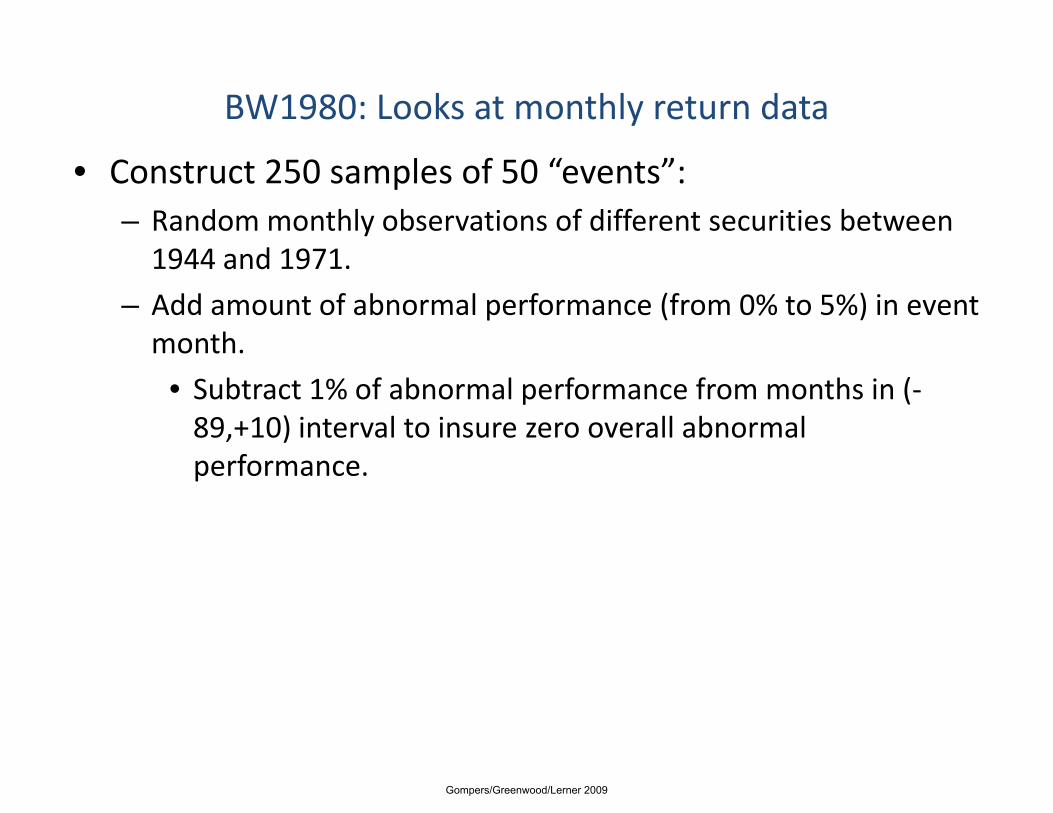
BW1980: Looks at monthly return data
• Construct 250 samples of 50 “events”:– Random monthly observations of different securities between 1944 d 19711944 and 1971.
– Add amount of abnormal performance (from 0% to 5%) in event month.
• Subtract 1% of abnormal performance from months in (‐89,+10) interval to insure zero overall abnormal
fperformance.
Gompers/Greenwood/Lerner 2009

BW 1980: Mean adjusted return
• Compute normalized return in month 0:
∑−
=111
iti RK ∑−= 8979 t
iti RK
2/1112)(
781)( ⎥
⎦
⎤⎢⎣
⎡−= ∑
−
iiti KRRσ89
)(78
)( ⎥⎦
⎢⎣
∑−−t
iiti
)(/)( iiitit RKRA σ−=
Gompers/Greenwood/Lerner 2009

BW 1980: Mean adjusted return (2)
• t‐test looks at whether A (the ratio of returns to variance) is anomalous:– Compare to the average A ratio for portfolio over (‐49,‐11) window:
• “Crude dependence adjustment ”Crude dependence adjustment.
– Could also compute the average of the variances:
• “No dependence adjustment.”
Gompers/Greenwood/Lerner 2009
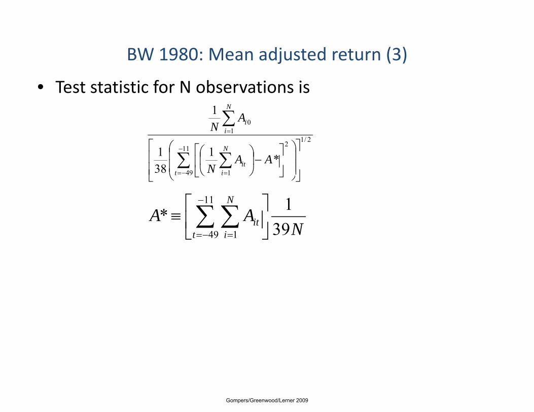
BW 1980: Mean adjusted return (3)
• Test statistic for N observations is
01 ∑
N
iAN
2/1211
49 1
1
*1381
⎥⎥
⎦
⎤
⎢⎢
⎣
⎡
⎟⎟
⎠
⎞
⎜⎜
⎝
⎛⎥⎦
⎤⎢⎣
⎡−⎟⎠
⎞⎜⎝
⎛∑ ∑−
−= =
=
t
N
iit
i
AAN
N
⎦⎣ ⎠⎝
NAA
N
iit 39
1*11
49 1⎥⎦
⎤⎢⎣
⎡≡ ∑ ∑
−
Nt i 3949 1 ⎦⎣ −= =
Gompers/Greenwood/Lerner 2009

BW 1980: Market adjusted return
• In this case, assume beta of one:– Somewhat simpler because no normalization for variance:
• Heteroscedasticity presumed to be less of a problem.
– Generally uses equal‐weighted index.
Otherwise identical– Otherwise identical.
mtitit RRA −=
Gompers/Greenwood/Lerner 2009

BW 1980: Market model adjusted return
• Estimate coefficients for market model using months in (‐89,‐11) interval.
• Define residual as Ait.
• Test statistic resembles market adjusted return:1 N
2/1211 11
10
11
1
⎟⎟⎞
⎜⎜⎛
⎥⎥⎤
⎢⎢⎡
⎟⎟⎞
⎜⎜⎛
⎟⎞
⎜⎛
−∑ ∑ ∑
∑− −
=
Nit
it
N
ii
AA
AN
1 89 89 7977 ⎟⎠
⎜⎝ ⎥
⎥⎦⎢
⎢⎣
⎟⎠
⎜⎝
⎟⎠
⎜⎝
∑ ∑ ∑= −= −=i t t
itN
Gompers/Greenwood/Lerner 2009
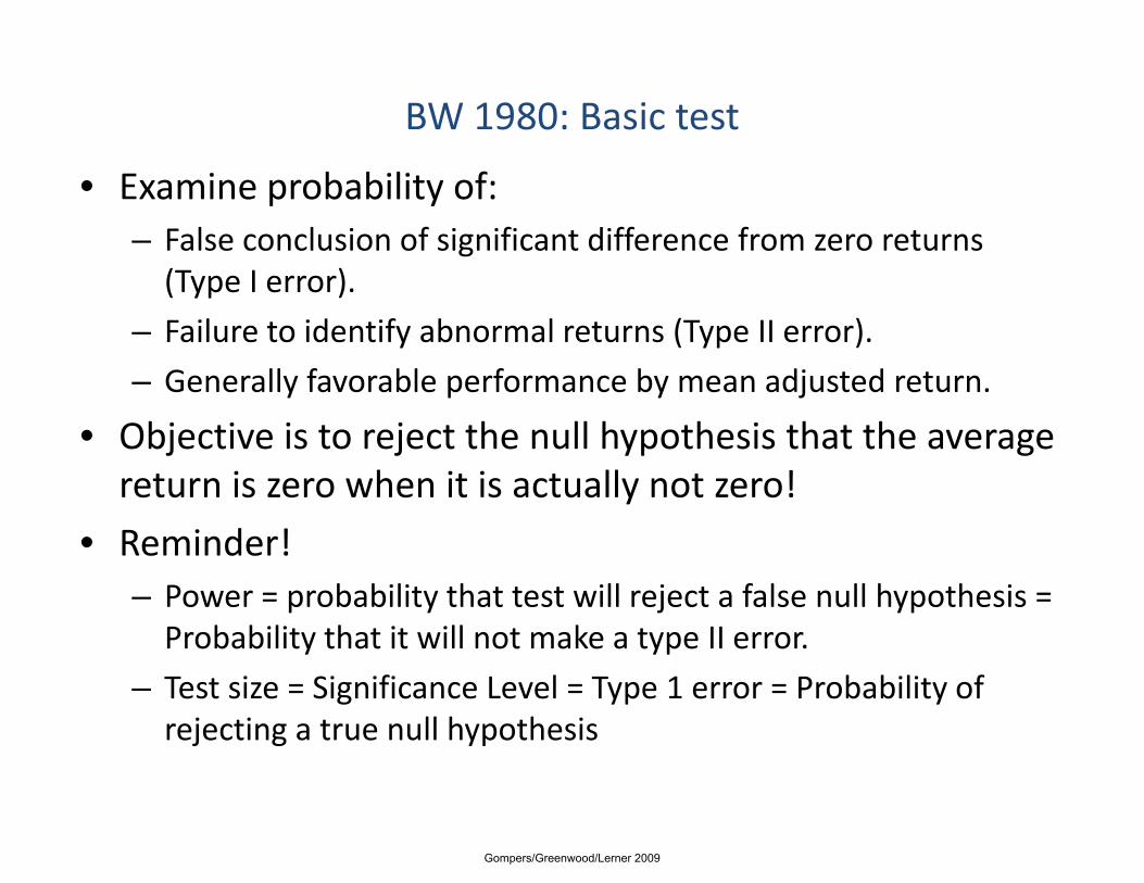
BW 1980: Basic test
• Examine probability of:– False conclusion of significant difference from zero returns (T I )(Type I error).
– Failure to identify abnormal returns (Type II error).
– Generally favorable performance by mean adjusted returnGenerally favorable performance by mean adjusted return.
• Objective is to reject the null hypothesis that the average return is zero when it is actually not zero!etu s e o e t s actua y ot e o
• Reminder!– Power = probability that test will reject a false null hypothesis = p y j ypProbability that it will not make a type II error.
– Test size = Significance Level = Type 1 error = Probability of j ti t ll h th irejecting a true null hypothesis
Gompers/Greenwood/Lerner 2009

Table 1: Main Results
Gompers/Greenwood/Lerner 2009
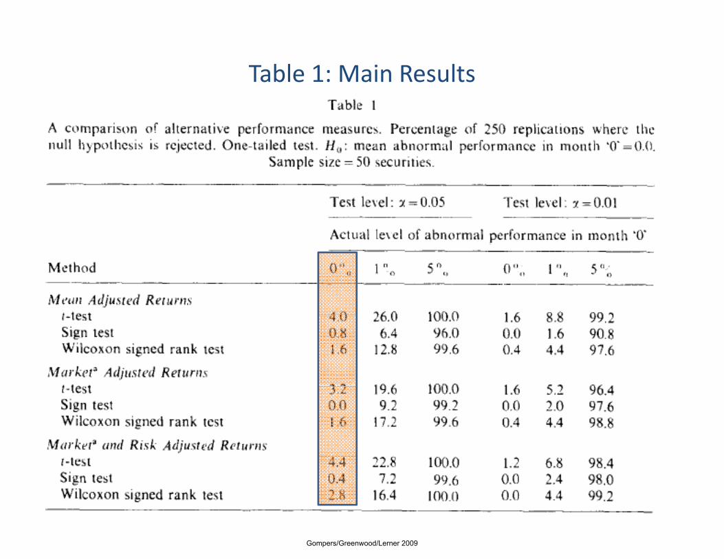
Table 1: Main Results
Gompers/Greenwood/Lerner 2009

Table 1: Main Results
Gompers/Greenwood/Lerner 2009

Table 1: Main Results
Gompers/Greenwood/Lerner 2009

BW 1980: Other results
• Dramatic fall‐off in power when uncertainty in event dates.
• When shifts in overall risk, market model adjustments may actually make worse off.
l h d d dd l l• Value‐weighted index adds little power.
Gompers/Greenwood/Lerner 2009
BW 1980: An important issue
• Many events are clustered in time, e.g.:– Merger waves.
– Regulatory shifts.
• Reduces degree of independence across observations.
• To test, induce event in same calendar month for each sample of 50 firms.
W k f f dj d i h• Weak performance of mean adjusted without dependence adjustment.
Gompers/Greenwood/Lerner 2009
BW 1980: Take‐aways
• In general, simplest methods work as well as more complex:– In some cases even better!
• Poor performance of mean‐adjusted returns when clusteringclustering.
• Getting event dates right is most critical!
Gompers/Greenwood/Lerner 2009

Brown and WarnerBrown and Warner
“Using Daily Stock Returns: The Case of Event Studies” [JFE, 1995].
Gompers/Greenwood/Lerner 2009

BW 1985: Repeats many of same analyses
• Rationale for new analysis:– Daily data has greater problems with non‐normality.
– Daily data has greater problems with non‐synchronous trading.
– Daily variance displays more non‐stationarity, serial dependencedependence.
Gompers/Greenwood/Lerner 2009
BW 1985: Same methodology
• 250 portfolios of 50 firms between 1962 and 1979.
• Gather data in (‐244,+5) window.
• Induce excess performance in event window.
• Compute the excess return measures (Ait) using three methods above.
Gompers/Greenwood/Lerner 2009
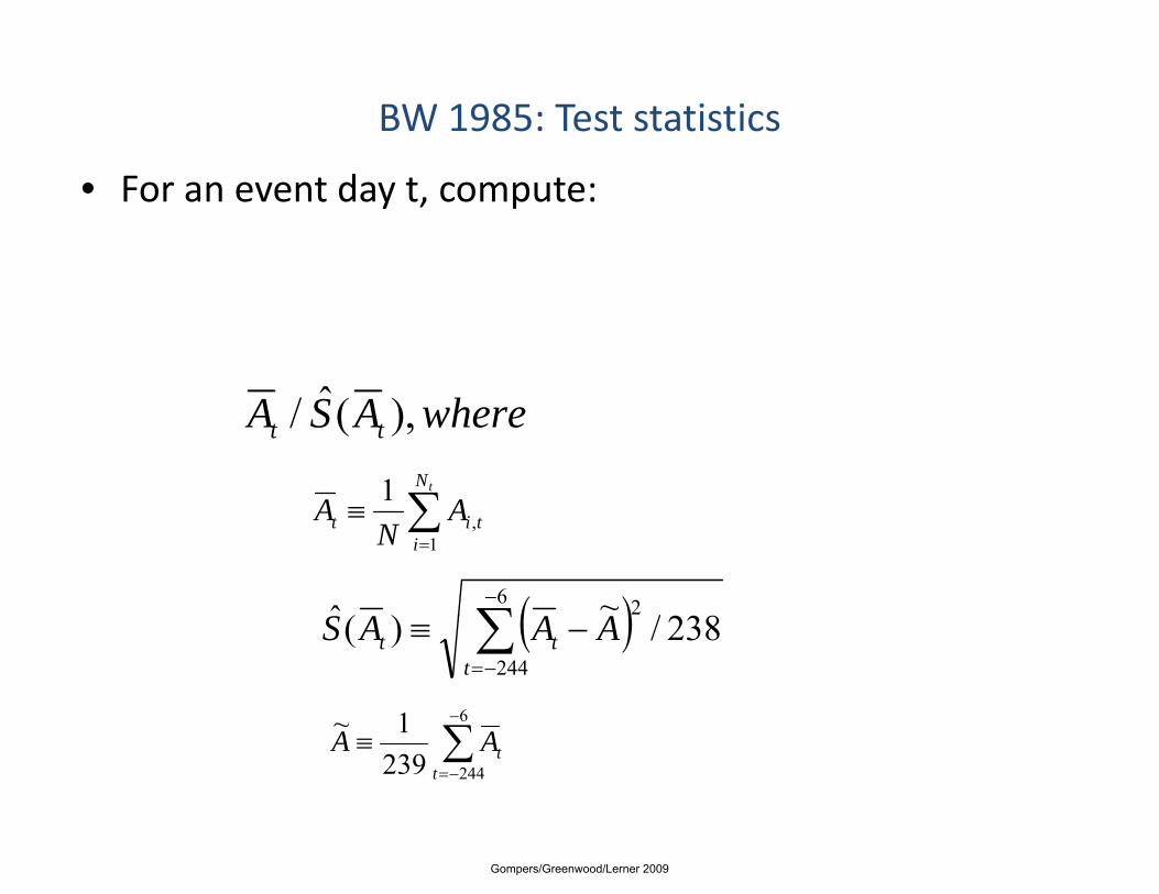
BW 1985: Test statistics
• For an event day t, compute:
ˆ whereASA tt ),(ˆ/
∑tN
AA 1 ∑=
≡i
tit AN
A1
,
( )∑−6 2
238/~)(ˆ AAAS ( )∑−=
−≡244
238/)(t
tt AAAS
∑−61~ ∑−=
≡244239
1t
tAA
Gompers/Greenwood/Lerner 2009

BW 1985: Basic tests
• Little difference between three methodologies.
• Considerable greater power than in monthly analysis (not surprising).
• Deterioration with longer event windows, smaller sample sizes.
Gompers/Greenwood/Lerner 2009
BW 1985: Other key analyses
• Clustering of events:– As before, deterioration in mean‐adjusted returns; little impact
th iotherwise.
• Non‐synchronous trading:Scholes Williams correction to market model makes little– Scholes‐Williams correction to market model makes little difference:
• While estimate of β is biased downward, estimate of α is βbiased upward!
Gompers/Greenwood/Lerner 2009
BW 1985: Take‐aways
• By and large, use of daily data is straightforward:– Little impact of non‐normality, controls for non‐synchronous t ditrading.
– Mean adjusted returns again perform worst.
– With longer windows may need to control for autocorrelation:With longer windows, may need to control for autocorrelation:
• But substantial loss of power.
Gompers/Greenwood/Lerner 2009

Bittlingmayer and HazlettBittlingmayer and Hazlett
“DOS Kapital” [JFE, 2000].
Gompers/Greenwood/Lerner 2009
Looks at market reaction to antitrust case
• “Stylized fact”: Microsoft harms competitors.
• Alternative explanations:– “Good competitor” that benefits other firms:
• E.g., network effects.
i h i i l d ffi i– Antitrust may thus impose social costs, end efficient behavior.
– Private harm but social benefit:Private harm but social benefit:
• Will not be able to discern this argument.
– Regulatory capture theory
Gompers/Greenwood/Lerner 2009

Explores effect on several classes of firms
• Microsoft itself.
• Firms that use Microsoft products:– Input prices should fall after suit.
• Firms that produce complementary products:– Increased demand.
• Rivals:– End of predatory behavior.
Gompers/Greenwood/Lerner 2009
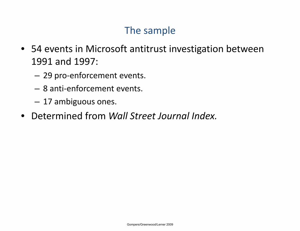
The sample
• 54 events in Microsoft antitrust investigation between 1991 and 1997:– 29 pro‐enforcement events.
– 8 anti‐enforcement events.
17 ambiguous ones– 17 ambiguous ones.
• Determined from Wall Street Journal Index.
Gompers/Greenwood/Lerner 2009
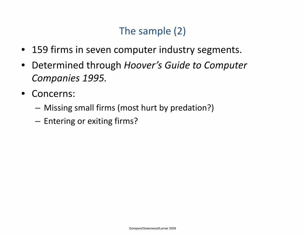
The sample (2)
• 159 firms in seven computer industry segments.
• Determined through Hoover’s Guide to Computer Companies 1995.
• Concerns:– Missing small firms (most hurt by predation?)
– Entering or exiting firms?
Gompers/Greenwood/Lerner 2009
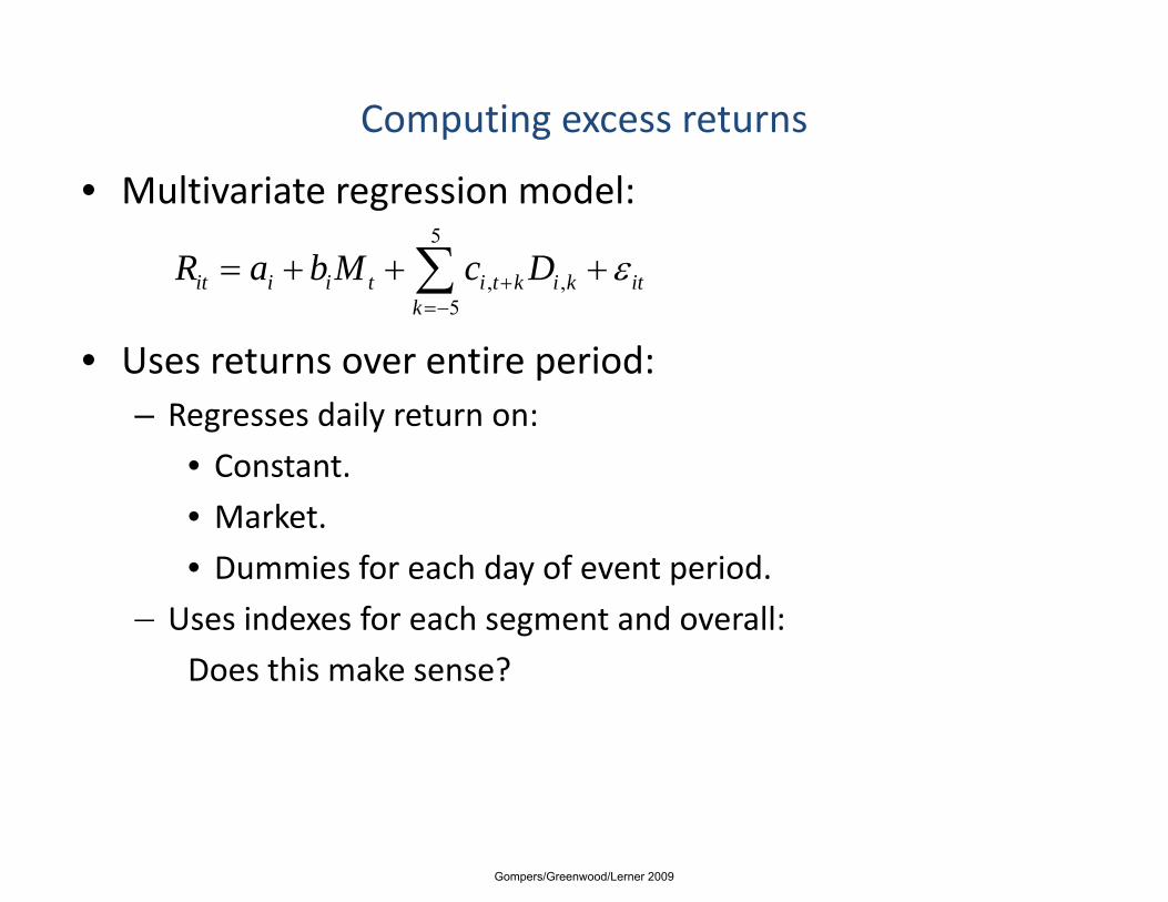
Computing excess returns
• Multivariate regression model:5
it i i t i t k i k itR a b M c D ε+= + + +∑
• Uses returns over entire period:
, ,5
it i i t i t k i k itk
+=−∑
– Regresses daily return on:
• Constant.
M k t• Market.
• Dummies for each day of event period.
– Uses indexes for each segment and overall:Uses indexes for each segment and overall:
Does this make sense?
Gompers/Greenwood/Lerner 2009

Computing excess returns
Estimate market beta
Event
“Multivariate” approachEffectively aggregates all ofEffectively aggregates all of These estimates
Gompers/Greenwood/Lerner 2009

Computing excess returns ‐ Limitations
Estimate market beta
Event
Some data gets underweighted
Some data gets overweighted
P bl ti l if thi k th t thProblematic only if we think that the beta is moving around a lot
Gompers/Greenwood/Lerner 2009
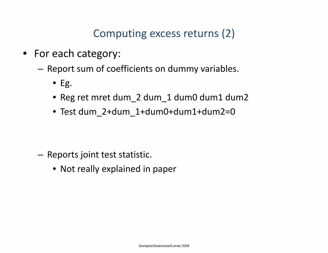
Computing excess returns (2)
• For each category:– Report sum of coefficients on dummy variables.
• Eg.
• Reg ret mret dum_2 dum_1 dum0 dum1 dum2
• Test dum 2+dum 1+dum0+dum1+dum2=0• Test dum_2+dum_1+dum0+dum1+dum2=0
– Reports joint test statistic.
• Not really explained in paper
Gompers/Greenwood/Lerner 2009

Overall effect
• Show positive gains on anti‐enforcement event announcements.
• Weaker, but significant, negative drop on pro‐enforcement event announcements.
h h f• Even stronger when restrict to events where Microsoft stock rose or fell.
Gompers/Greenwood/Lerner 2009

Looking for social welfare harm
• Seek events where 1.5σ reactions of Microsoft, index, in opposite directions:– Is there any evidence of change in social welfare here.
• Only a few events‐‐19 in all!
(• Almost all firm‐specific events (earnings announcements, other litigation, etc.)
P id littl t f l i• Provides little support for claims.
Gompers/Greenwood/Lerner 2009
d l d
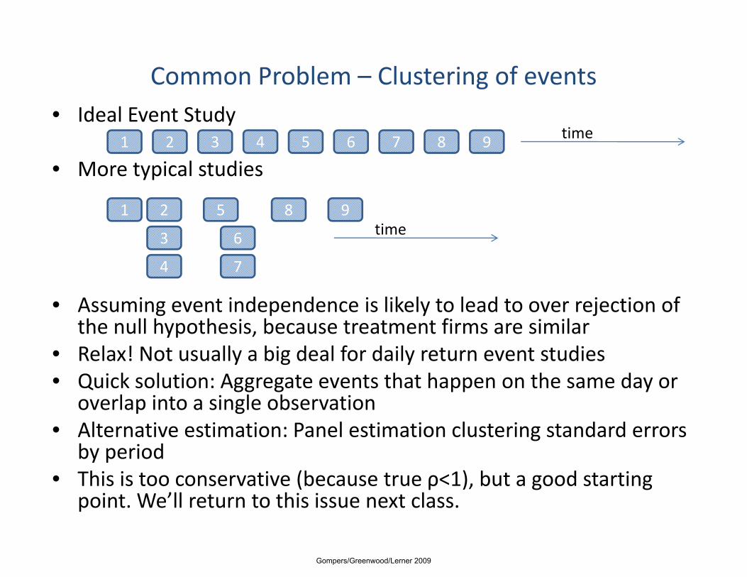
Common Problem – Clustering of events• Ideal Event Study
• More typical studies1 2 3 4 5 6 7 8 9 time
yp
1 2
3
5
6
8 9time
• Assuming event independence is likely to lead to over rejection of the null hypothesis because treatment firms are similar
4 7
the null hypothesis, because treatment firms are similar• Relax! Not usually a big deal for daily return event studies• Quick solution: Aggregate events that happen on the same day or
l i t i l b tioverlap into a single observation• Alternative estimation: Panel estimation clustering standard errors
by periodh (b ) b d• This is too conservative (because true ρ<1), but a good starting point. We’ll return to this issue next class.
Gompers/Greenwood/Lerner 2009

GreenwoodGreenwood
“Short‐ and Long‐term demand curves for stocks: Theory and Evidence on the dynamics of arbitrage” [JFE, 2005].
Gompers/Greenwood/Lerner 2009

Event Summary
• Reweighting of Nikkei 225 Index• Nikkei index equal to sum of prices of constituents divided by index
divisor• 30 Additions experience positive demand shock, 30 deletions
negative demand shock, 195 remainders negative demand shock• Under assumption of 2 430 billion yen of index linked assets• Under assumption of 2,430 billion yen of index linked assets,
rebalancing caused 2,000 billion yen of trading in one week (~ $US 20 billion).
• Substantial variation in demand shocks between stocks:• By Yen size of shock• Max 127 billion Yen Min 221 million YenMax 127 billion Yen, Min 221 million Yen• As a fraction of market capitalization• One deletion experienced a shock equivalent to 17.59% of its
k lmarket capitalization• One additions experienced a shock equivalent to 9.61% of its
market capitalizationGompers/Greenwood/Lerner 2009

A Single Event
Pre-event w indow Event window Post-event window
April 14 Friday
April 17 Monday
April 21Friday
April 24 Monday
Announcement day
Institutions begin rebalancing
Bulk ofinstitutions
are expected to rebalance
on this day
At close,30 index
stocks
stocksreplaced
Gompers/Greenwood/Lerner 2009

Unusual Features of Event
• 30 Adds, 30 Deletes, 195 Remainders• Adds = 30% of new index, Deletes = 3% of old index• Implication: Remainders get significantly downweightedImplication: Remainders get significantly downweighted• Can compute cumulative returns for each of these portfolios:
30
10
20
etur
n
Additions
10
0April 7, 2000 April 17, 2000 April 27, 2000 May 7, 2000
e Pe
rcen
tage
Re
TOPIX
R i d
-20
-10
Cum
ulat
iv Remainders
-40
-30
Gompers/Greenwood/Lerner 2009

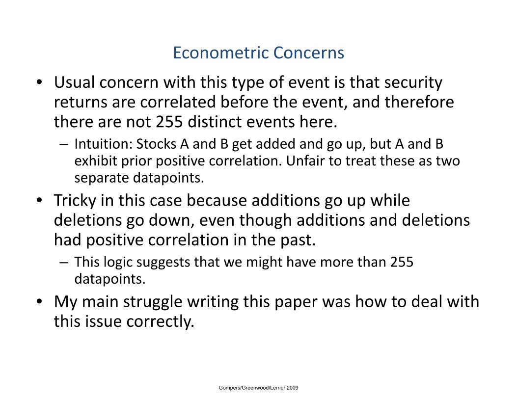
Econometric Concerns
• Usual concern with this type of event is that security returns are correlated before the event, and therefore there are not 255 distinct events herethere are not 255 distinct events here.– Intuition: Stocks A and B get added and go up, but A and B exhibit prior positive correlation. Unfair to treat these as two
t d t i tseparate datapoints.
• Tricky in this case because additions go up while deletions go down, even though additions and deletionsdeletions go down, even though additions and deletions had positive correlation in the past.– This logic suggests that we might have more than 255 d t i tdatapoints.
• My main struggle writing this paper was how to deal with this issue correctly.this issue correctly.
Gompers/Greenwood/Lerner 2009

Theory 1
• Capital Market includes N risky securities in fixed supply given by supply vector Q.
t
∑• Consider a mean variance world, where risk averse
b h f
, ,0 ,1
i t i i ss
D D ε=
= +∑
arbitrageurs have mean variance preferences over next period’s returns.
max [ exp( )]E Wγ
ld d
1'
1 1
max [ exp( )]
[ ]N t t
t t t t t
E W
W W N P P
γ +
+ +
− −
= + −
• Yields Demand1
1 11 [ ( )] ( ( ) ).t t t t t tN Var P E P Pγ
−+ += −
• With supply Qγ
1 1( ) ( ) .t t t t tP E P Var P Qγ+ += −Gompers/Greenwood/Lerner 2009
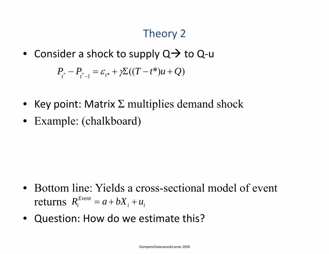
Theory 2
• Consider a shock to supply Q to Q‐u
* * *1(( *) )tt t
P P T t u Qε γ−
− = + Σ − +
• Key point: Matrix Σ multiplies demand shock• Example: (chalkboard)
• Bottom line: Yields a cross-sectional model of event returns Event
i i iR a bX u= + +
• Question: How do we estimate this?
Gompers/Greenwood/Lerner 2009
Econometric Concerns
• Usual concern with this type of event is that security returns are correlated before the event, and therefore there are not 255 distinct events herethere are not 255 distinct events here.– Intuition: Stocks A and B get added and go up, but A and B exhibit prior positive correlation. Unfair to treat these as two
t d t i tseparate datapoints.
• Tricky in this case because additions go up while deletions go down, even though additions and deletionsdeletions go down, even though additions and deletions had positive correlation in the past.– This logic suggests that we might have more than 255 d t i tdatapoints.
• My main struggle writing this paper was how to deal with this issue correctly.this issue correctly.
Gompers/Greenwood/Lerner 2009

Solution: GLS? GLS standard errors?
• Recall the OLS Estimator minimizes2( ) ' ( )y X y Xβ σ β− −
• Yielding estimator1( ' ) ( ' )X X X yβ −=
I went with OLS estimatorWith GLS standard errorsGuiding principle: OLS
• But if instead we think that ( )Var ε = Σ
Guiding principle: OLS Estimates are not sensitiveTo covariance matrix. However, we want to be C ti i
• Then we want the GLS estimator1 1 1( ' ) ( ' )X X X yβ − − −= Σ Σ
Conservative in our Standard errors.
• With standard errors given by1( ) ( ' )Var X Xβ −= Σ( ) ( )Var X Xβ Σ
Gompers/Greenwood/Lerner 2009

Solution: GLS? GLS standard errors?
• Recall the OLS Estimator minimizes2( ) ' ( )y X y Xβ σ β− −
• Yielding estimator1( ' ) ( ' )X X X yβ −=
Roughly speaking, t‐statsGo down from about 10To range of 3 or 4
• But if instead we think that ( )Var ε = Σ
To range of 3 or 4
• Then we want the GLS estimator1 1 1( ' ) ( ' )X X X yβ − − −= Σ Σ
• With standard errors given by1( ) ( ' )Var X Xβ −= Σ( ) ( )Var X Xβ Σ
Gompers/Greenwood/Lerner 2009

Figure 5
Gompers/Greenwood/Lerner 2009

Figure 5Looks like a t‐stat of 30…But GLS adjustment takes it down considerably
Gompers/Greenwood/Lerner 2009
Gompers/Greenwood/Lerner 2009

“Comovement”
Nicholas Barberis – Chicago and NBER
Andrei Shleifer – Harvard and NBERAndrei Shleifer Harvard and NBER
Jeffrey Wurgler – NYU Stern
JFE 2004
Gompers/Greenwood/Lerner 2009
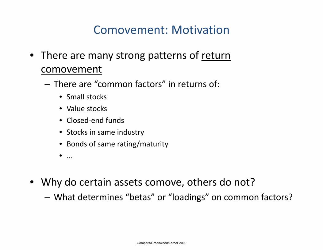
Comovement: Motivation
• There are many strong patterns of return comovement– There are “common factors” in returns of:
• Small stocks
• Value stocksValue stocks
• Closed‐end funds
• Stocks in same industry
/• Bonds of same rating/maturity
• ...
• Why do certain assets comove, others do not?– What determines “betas” or “loadings” on common factors?
Gompers/Greenwood/Lerner 2009

Comovement: Motivation 2
• Traditional view: Fundamentals‐based comovement– Assets comove because their “fundamental values” comove
– A very useful paradigm… but the whole story?
S li id• Some puzzling evidence– Siamese‐twin stocks
– Closed‐end country funds
– Small stocks, value stocks
– Commodities
• Alternative view: Trading‐driven comovement – In addition to fundamentals
Gompers/Greenwood/Lerner 2009
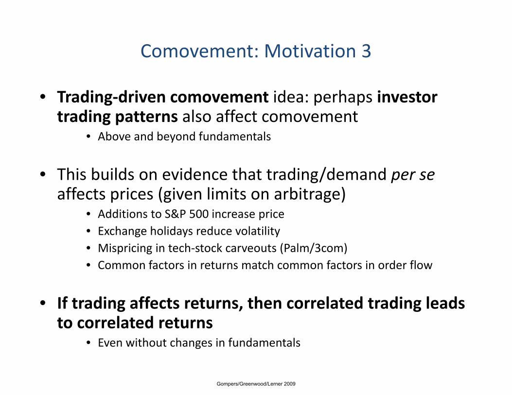
Comovement: Motivation 3
• Trading‐driven comovement idea: perhaps investor trading patterns also affect comovementg p
• Above and beyond fundamentals
• This builds on evidence that trading/demand per se• This builds on evidence that trading/demand per seaffects prices (given limits on arbitrage)
• Additions to S&P 500 increase price• Exchange holidays reduce volatility• Mispricing in tech‐stock carveouts (Palm/3com)• Common factors in returns match common factors in order flow
• If trading affects returns, then correlated trading leads to correlated returnsto correlated returns
• Even without changes in fundamentals
Gompers/Greenwood/Lerner 2009

Comovement: Conjectures
• Trading‐induced comovement models make 3 predictions
• H1: Suppose asset j, previously a member of Y, gets reclassified into X. Then j’s univariate beta w.r.t. the X index will increase, as will its R2 w.r.t. X index.,
• H2: Suppose asset j, previously a member of Y, gets reclassified into X. Then j’s bivariate beta w.r.t. X will increase, and its bivariate beta w.r.t. Y will decrease.
• H3: More and more noise traders (who use X and Y as categories/habitats) mean less and less correlation between X and Y.
Gompers/Greenwood/Lerner 2009

Tests: Event Study
• Setting: S&P 500 additions and deletions– S&P 500 is a category/habitat/classification used by many investors– Membership changes don’t have obvious info. about fundamentals– X = S&P 500– Y = non‐S&P 500 (complement)
• H1: Does univariate S&P beta goes up following addition?• Yes (in daily & weekly returns, but not monthly): Table 1
• H2: Following addition, does bivariate S&P beta go up, non‐S&P beta go down?
• Yes (at every horizon) – Figure 1Yes (at every horizon) Figure 1
• H3: Is correlation between S&P, non‐S&P declining over time (possibly reflecting index fund growth)?(possibly reflecting index fund growth)?
• Yes – Table 4
Gompers/Greenwood/Lerner 2009

Table 1
Gompers/Greenwood/Lerner 2009
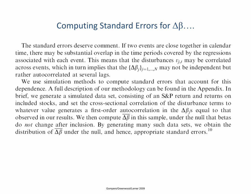
Computing Standard Errors for Δβ….
Gompers/Greenwood/Lerner 2009
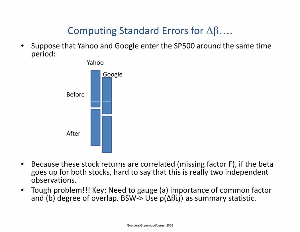
Computing Standard Errors for Δβ….h h d l h d h• Suppose that Yahoo and Google enter the SP500 around the same time
period:Yahoo
G lGoogle
Before
After
• Because these stock returns are correlated (missing factor F), if the beta goes up for both stocks, hard to say that this is really two independent observations.
• Tough problem!!! Key: Need to gauge (a) importance of common factor• Tough problem!!! Key: Need to gauge (a) importance of common factor and (b) degree of overlap. BSW‐> Use ρ(Δβij) as summary statistic.
Gompers/Greenwood/Lerner 2009
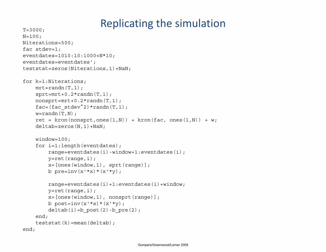
Replicating the simulationT=3000;N=100;Niterations=500;fac stdev=1;eventdates=1010:10:1000+N*10;eventdates=eventdates';teststat=zeros(Niterations,1)+NaN;
for k=1:Niterations;mrt=randn(T,1);sprt=mrt+0.2*randn(T,1);nonsprt=mrt+0.2*randn(T,1);fac=(fac_stdev^2)*randn(T,1);w=randn(T,N);ret = kron(nonsprt,ones(1,N)) + kron(fac, ones(1,N)) + w;deltab=zeros(N,1)+NaN;
window=100;for i=1:length(eventdates);
range=eventdates(i)-window+1:eventdates(i);y=ret(range,i);x=[ones(window,1), sprt(range)];b pre=inv(x'*x)*(x'*y);p y
range=eventdates(i)+1:eventdates(i)+window;y=ret(range,i);x=[ones(window,1), nonsprt(range)];b post=inv(x'*x)*(x'*y); p ( ) ( y);deltab(i)=b_post(2)-b_pre(2);
end;teststat(k)=mean(deltab);
end;
Gompers/Greenwood/Lerner 2009
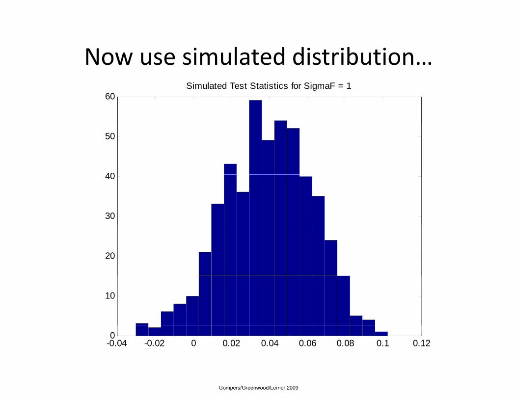
Now use simulated distribution…60
Simulated Test Statistics for SigmaF = 1
40
50
30
40
20
10
-0.04 -0.02 0 0.02 0.04 0.06 0.08 0.1 0.120
Gompers/Greenwood/Lerner 2009
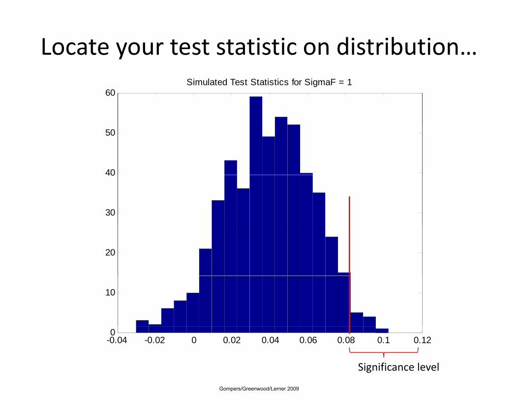
Locate your test statistic on distribution…
60Simulated Test Statistics for SigmaF = 1
40
50
30
40
20
10
-0.04 -0.02 0 0.02 0.04 0.06 0.08 0.1 0.120
Significance level
Gompers/Greenwood/Lerner 2009

Event Studies – Summary and Extensions
Gompers/Greenwood/Lerner 2009
Methodological refinements
• Tests above make assumptions about distribution that may be unappealing.
• Non‐parametric tests address this concern by looking at sign, ranking.
b ll d l [ ] h• Campbell and Wasley [1993] argue that non‐parametric tests provide more robust conclusions than parametric onesones.
• When you are worried about the distribution, usually not that difficult to simulatethat difficult to simulate
Gompers/Greenwood/Lerner 2009
Other methodological refinements (2)
• Often event day is uncertain, e.g.:– Wall Street Journal Index entries.
– SEC filings.
• Can approach in two ways:d i d– Expand event window.
– Model uncertainty in maximum likelihood framework [Ball and Torous, 1988].Torous, 1988].
• Unclear how much extra power more painful ML approach brings.
Gompers/Greenwood/Lerner 2009

Open issues
• Exogeneity of corporate announcements:– Many decisions (e.g., acquisitions) are under the control of
tmanagement.
– They can be expected to be “timed” to fall when they have maximum positive impact on stock price.p p p
– Simple analyses may thus be biased.
Gompers/Greenwood/Lerner 2009

Illustration
• Eckbo, Maksimovic, and Williams [1990] look at announcements of corporate acquisitions.– Estimate “naïve” OLS regressions, as well as maximum likelihood regressions that account for timing of decision:
• With OLS extent of synergies in acquisition do not explainWith OLS, extent of synergies in acquisition do not explain size of reaction.
• Once ML is used, explanatory power of synergy measures increase dramatically.
Gompers/Greenwood/Lerner 2009

Open issues (2)
• Many announcements are at least partially anticipated by the market.
• Danger in cross‐sectional analyses:– May interpret characteristics as being related to event impact.
A ll b l d f di l– Actually, may be related to extent of disclosure.
Gompers/Greenwood/Lerner 2009

Illustration
• Austin [AER, 1993] examines whether market rationally responds to patent awards.
• Concludes that it does:– Patent awards listed in Wall Street Journal have greater importance and more positive reactionimportance and more positive reaction.
– But published patents may also represent more “news.”
Gompers/Greenwood/Lerner 2009
Conclusions
• Contrast to studies of long‐run returns:– Well agreed‐upon methodology.
– Theoretical foundations.
• Huge published literature suggests that most “low‐h i f it” h b l k dhanging fruit” has been plucked
• Continuing opportunities on finance‐economics interfaceinterface.
Gompers/Greenwood/Lerner 2009
Next Class
• Long horizon returns– Applications:
• Security offerings and repurchases
• M&A
• Settings where market efficiency is being called into• Settings where market efficiency is being called into question
• CARs versus BHARs versus Wealth Ratios
• Panel data approaches to clustering when events overlappp g p
• Calendar time regression approaches
Gompers/Greenwood/Lerner 2009