computational methods for quantitative finance
TRANSCRIPT
PreliminariesPricing by binomial tree method
Computational Methods for Quantitative FinanceModels, Algorithms, Numerical Analysis
Christoph SchwabN. Hilber, C. Winter
ETHZ-UNIZ Master of Advanced Studies in Finance
Spring Term 2008
Christoph Schwab Computational Methods for Quantitative Finance
PreliminariesPricing by binomial tree method
Scope of the course
Analysis and implementation of numerical methods forpricing options.
Models: Black-Scholes, stochastic volatility, exponential Levy.
Options: European, American, Asian, barrier, compound . . .
In this course: Focus on deterministic (PDE based) methods
I binomial and multinomial trees
I Finite Difference methods
I Finite Element methods
This course will be continued by the course Monte Carlo methodsin autumn 2008.
Christoph Schwab Computational Methods for Quantitative Finance

PreliminariesPricing by binomial tree method
Organization of the course
13 lectures (2 hours) + 12 exercise classes (1 hour).
I No lectures on March, 27. and May, 1.
I No exercise class on March, 25.
I Testat: 75% of solved homework assignments(theoretical exercises + MATLAB programming).
Examination: On Thursday, May 29, 10–12.Written, closed-book examination includes theoretical andMATLAB programming problems.Examination takes place on ETH-workstations running MATLABunder LINUX. Own computer will NOT be required.
Christoph Schwab Computational Methods for Quantitative Finance

PreliminariesPricing by binomial tree method
Details of the course
I Elementary Pricing
1. Pricing by binomial trees2. Pricing by Finite Difference Solution of PDEs3. American options4. Barrier and Asian contracts
II Pricing by Finite Element methods
5. Variational Formulation of BS model6. Finite Element Methods for infinite horizon problems7. Time stepping for finite horizon European vanillas8. Finite horizon American contracts
III Pricing in incomplete markets
9. Stochastic volatility models10. Levy models
Christoph Schwab Computational Methods for Quantitative Finance

PreliminariesPricing by binomial tree method
OptionsStochastic processesBlack-Scholes model
Outline
PreliminariesOptionsStochastic processesBlack-Scholes model
Pricing by binomial tree methodBinomial tree modelMatlab implementation: Euro1.m–Euro9.m
Christoph Schwab Computational Methods for Quantitative Finance

PreliminariesPricing by binomial tree method
OptionsStochastic processesBlack-Scholes model
Definition
An option is a contract which gives the right (but not theobligation) to buy or to sell a risky asset at a specified date T inthe future (or within a specified period) at a specified price K.
T : maturity or expiry date (after T the option is worthless)
K: strike or exercise price
Options are derivative contracts.
Examples of underlying assets (or underlyings): stocks (shares ofa company), indices (weighted means of several stocks), bonds,currencies, other options . . .
Christoph Schwab Computational Methods for Quantitative Finance
PreliminariesPricing by binomial tree method
OptionsStochastic processesBlack-Scholes model
Examples
Call: right to buy the underlying
Put: right to sell the underlying
Exercise styles
I European: exercise only at maturity T
I American: exercise at any date before the maturity T(the holder chooses when exercise the option)
More complicated, exotic (as opposed to simple vanilla) options:
I Barrier: depend on particular asset price level(s) attained over a period
I Asian: depend on the average price of the underlying over a period
I Lookback: depend on the minimum or maximum asset price over a period
(⇒ path-dependent options)
Christoph Schwab Computational Methods for Quantitative Finance

PreliminariesPricing by binomial tree method
OptionsStochastic processesBlack-Scholes model
Value of an option
The right without obligations is not given for free: option has avalue called premium (do not confuse with the exercise price K!)
What is the fair price of an option? It depends on:
I Assumptions on the market
I Model for the underlying price
Note: the price of standard liquid options is defined by the market(offer-demand equilibrium). Models are mostly needed forvaluation of exotic options.
Christoph Schwab Computational Methods for Quantitative Finance
PreliminariesPricing by binomial tree method
OptionsStochastic processesBlack-Scholes model
Modelling assumptions on the market
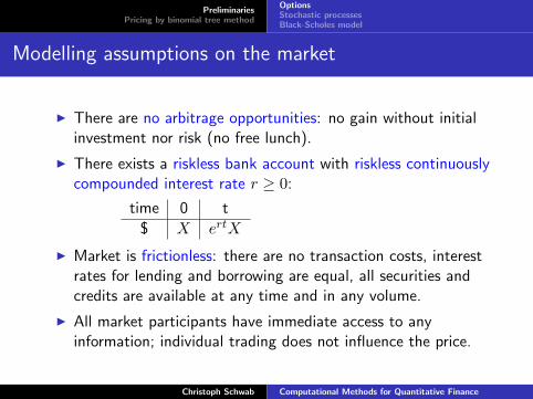
I There are no arbitrage opportunities: no gain without initialinvestment nor risk (no free lunch).
I There exists a riskless bank account with riskless continuouslycompounded interest rate r ≥ 0:
time 0 t
$ X ertX
I Market is frictionless: there are no transaction costs, interestrates for lending and borrowing are equal, all securities andcredits are available at any time and in any volume.
I All market participants have immediate access to anyinformation; individual trading does not influence the price.
Christoph Schwab Computational Methods for Quantitative Finance
PreliminariesPricing by binomial tree method
OptionsStochastic processesBlack-Scholes model
Payoff function
The payoff of an option is its value at the time of exercise.The payoff is a function of the underlying price S at this time.
Examples:
I Call: max(S −K, 0) ≡ (S −K)+.
I Put: max(K − S, 0) ≡ (K − S)+.
Note: the payoff function can be obtained by no arbitrageargument. It does not depend on the model for the underlyingprice.On the contrary, to find values of the option before the exercise, wehave to do some assumptions on the evolution of the asset price.
Christoph Schwab Computational Methods for Quantitative Finance
PreliminariesPricing by binomial tree method
OptionsStochastic processesBlack-Scholes model
Stochastic modelling of the stock price
Stock prices in the future are not known: they are modelled bystochastic processes.
A stochastic process (St)t∈[0,T ] is a random function of t.
Filtered probability space: (Ω,F ,P, (Ft)t∈[0,T ]).
I Ω: set of elementary events ω
I F : σ-algebra of all events (i.e. subsets of Ω)
I P: probability measure on FI (Ft)t∈[0,T ] (filtration): increasing family of σ-algebras.Ft represents the information available up to time t.
(St(ω))t∈[0,T ] is a trajectory or sample path of the process.
Christoph Schwab Computational Methods for Quantitative Finance
PreliminariesPricing by binomial tree method
OptionsStochastic processesBlack-Scholes model
Important definitions
A stochastic process X is adapted (w.r.t. the filtration) if Xt isFt-measurable (notation: Xt ∈ Ft).It means that the value of Xt is revealed at time t.
X is a Markov process if, for any bdd Borel function f and ∀s ≥ t,E[f(Xs) | Ft] = E[f(Xs) |Xt]:the future values of X do not depend on the past but only on thepresent value.
An adapted process X is a martingale if
(i) E[|Xt|] <∞ for all t ≥ 0(ii) E[Xs | Ft] = Xt, for all s ≥ t
(the best prediction for future values is the present value).
X is cadlag if its trajectories Xt(ω) are almost surely rightcontinuous and have left limits at all t ∈ [0, T ].French: continu a droite, limite a gauche.
Christoph Schwab Computational Methods for Quantitative Finance
PreliminariesPricing by binomial tree method
OptionsStochastic processesBlack-Scholes model
Brownian motion
Normal distribution N (µ, σ2) has the density
f(x) = 1√2πσ2
exp(− (x−µ)2
2σ2
).
A stochastic process W is a Wiener process or Brownian motion if
I W0 = 0 a.s.
I W has independent increments: for all t1 ≤ t2 ≤ t3 ≤ t4,Wt4 −Wt3 ⊥⊥Wt2 −Wt1 .
I increments of W are normally distributed:Wt+s −Wt ∼ N (0, s).
Properties:
I Wiener process is a Markov process and a martingale.
I Wt ∼ N (0, t), E[Wt] = 0, VarWt = t.
I W has continuous paths.
Christoph Schwab Computational Methods for Quantitative Finance
PreliminariesPricing by binomial tree method
OptionsStochastic processesBlack-Scholes model
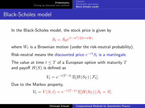
Black-Scholes model
In the Black-Scholes model, the stock price is given by
St = S0e(r−σ2/2)t+σWt
where Wt is a Brownian motion (under the risk-neutral probability).
Risk-neutral means the discounted price e−rtSt is a martingale.
The value at time t ≤ T of a European option with maturity Tand payoff H(S) is defined as
Vt = e−r(T−t) E[H(ST ) | Ft].Due to the Markov property,
Vt = V (S, t) = e−r(T−t) E[H(ST ) |St = S].
Christoph Schwab Computational Methods for Quantitative Finance
PreliminariesPricing by binomial tree method
OptionsStochastic processesBlack-Scholes model
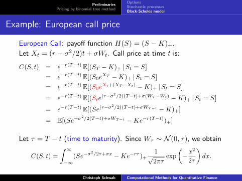
Example: European call price
European Call: payoff function H(S) = (S −K)+.
Let Xt = (r − σ2/2)t+ σWt. Call price at time t is:
C(S, t) = e−r(T−t) E[(ST −K)+ |St = S]= e−r(T−t) E[(S0e
XT −K)+ |St = S]= e−r(T−t) E[(S0e
Xt+(XT−Xt) −K)+ |St = S]
= e−r(T−t) E[(Ste(r−σ2/2)(T−t)+σ(WT−Wt) −K)+ |St = S]
= e−r(T−t) E[(Se(r−σ2/2)(T−t)+σWT−t −K)+]
= E[(Se−σ2/2(T−t)+σWT−t −Ke−r(T−t))+]
Let τ = T − t (time to maturity). Since Wτ ∼ N (0, τ), we obtain
C(S, t) =∫ ∞−∞
(Se−σ2/2τ+σx −Ke−rτ )+
1√2πτ
exp(−x
2
2τ
)dx.
Christoph Schwab Computational Methods for Quantitative Finance
PreliminariesPricing by binomial tree method
OptionsStochastic processesBlack-Scholes model
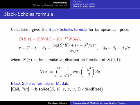
Black-Scholes formula
Calculation gives the Black-Scholes formula for European call price:
C(S, t) = S N(d1)−Ke−rτN(d2),
τ = T − t, d1 =log(S/K) + (r + σ2/2)τ
σ√τ
, d2 = d1 − σ√τ
where N(x) is the cumulative distribution function of N (0, 1):
N(x) =∫ x
−∞1√2π
exp(−y
2
2
)dy.
Black-Scholes formula in Matlab:
[Call, Put] = blsprice(S, K, r, τ , σ, DividendRate)
Christoph Schwab Computational Methods for Quantitative Finance
PreliminariesPricing by binomial tree method
Binomial tree modelMatlab implementation: Euro1.m–Euro9.m
Outline
PreliminariesOptionsStochastic processesBlack-Scholes model
Pricing by binomial tree methodBinomial tree modelMatlab implementation: Euro1.m–Euro9.m
Christoph Schwab Computational Methods for Quantitative Finance
PreliminariesPricing by binomial tree method
Binomial tree modelMatlab implementation: Euro1.m–Euro9.m
Model setting
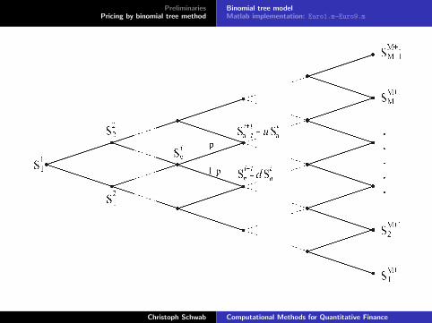
We construct a simple discrete time model:
I M time steps: 0 = t1 < t2 < · · · < tM < tM+1 = T ,ti = (i− 1)∆t, i = 1, . . . ,M + 1, ∆t = T/M .
I At each time step there are only two possibilities for the price:S Su with probability p or S Sd with probability 1− p,d < 1 < u.
Parameters u, d, and p will be chosen such that the binomialmodel converges to the Black-Scholes model as M →∞.
Christoph Schwab Computational Methods for Quantitative Finance
PreliminariesPricing by binomial tree method
Binomial tree modelMatlab implementation: Euro1.m–Euro9.m
Christoph Schwab Computational Methods for Quantitative Finance
PreliminariesPricing by binomial tree method
Binomial tree modelMatlab implementation: Euro1.m–Euro9.m
Choice of parameters u, d, p
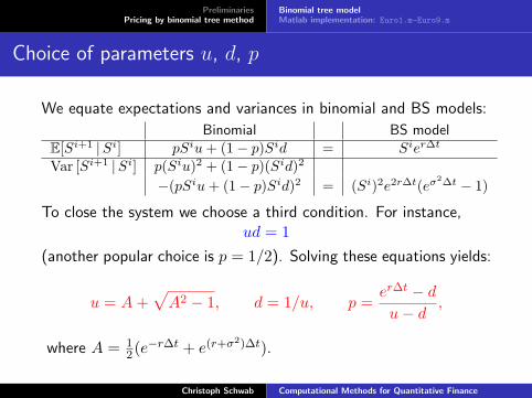
We equate expectations and variances in binomial and BS models:
Binomial BS modelE[Si+1 |Si] pSiu+ (1− p)Sid = Sier∆t
Var [Si+1 |Si] p(Siu)2 + (1− p)(Sid)2
−(pSiu+ (1− p)Sid)2 = (Si)2e2r∆t(eσ2∆t − 1)
To close the system we choose a third condition. For instance,ud = 1
(another popular choice is p = 1/2). Solving these equations yields:
u = A+√A2 − 1, d = 1/u, p =
er∆t − du− d ,
where A = 12(e−r∆t + e(r+σ2)∆t).
Christoph Schwab Computational Methods for Quantitative Finance
PreliminariesPricing by binomial tree method
Binomial tree modelMatlab implementation: Euro1.m–Euro9.m
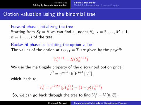
Option valuation using the binomial tree
Forward phase: initializing the treeStarting from S1
1 = S we can find all nodes Sin, i = 2, . . . ,M + 1,n = 1, . . . , i of the tree.
Backward phase: calculating the option valuesThe values of the option at tM+1 = T are given by the payoff:
VM+1n = H(SM+1
n )
We use the martingale property of the discounted option price:
V i = e−r∆t E[V i+1 |V i]which leads to
V in = e−r∆t (pV i+1
n+1 + (1− p)V i+1n )
So, we can go back through the tree to find V 11 = V (0, S).
Christoph Schwab Computational Methods for Quantitative Finance
PreliminariesPricing by binomial tree method
Binomial tree modelMatlab implementation: Euro1.m–Euro9.m
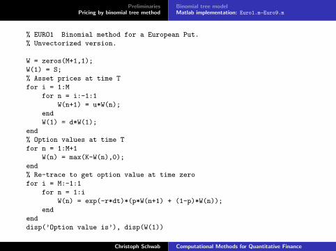
% EURO1 Binomial method for a European Put.
% Unvectorized version.
W = zeros(M+1,1);
W(1) = S;
% Asset prices at time T
for i = 1:M
for n = i:-1:1
W(n+1) = u*W(n);
end
W(1) = d*W(1);
end
% Option values at time T
for n = 1:M+1
W(n) = max(K-W(n),0);
end
% Re-trace to get option value at time zero
for i = M:-1:1
for n = 1:i
W(n) = exp(-r*dt)*(p*W(n+1) + (1-p)*W(n));
end
end
disp(’Option value is’), disp(W(1))
Christoph Schwab Computational Methods for Quantitative Finance
PreliminariesPricing by binomial tree method
Binomial tree modelMatlab implementation: Euro1.m–Euro9.m
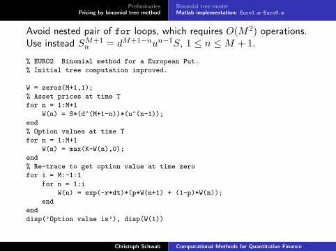
Avoid nested pair of for loops, which requires O(M2) operations.Use instead SM+1
n = dM+1−nun−1S, 1 ≤ n ≤M + 1.
% EURO2 Binomial method for a European Put.
% Initial tree computation improved.
W = zeros(M+1,1);
% Asset prices at time T
for n = 1:M+1
W(n) = S*(d^(M+1-n))*(u^(n-1));
end
% Option values at time T
for n = 1:M+1
W(n) = max(K-W(n),0);
end
% Re-trace to get option value at time zero
for i = M:-1:1
for n = 1:i
W(n) = exp(-r*dt)*(p*W(n+1) + (1-p)*W(n));
end
end
disp(’Option value is’), disp(W(1))
Christoph Schwab Computational Methods for Quantitative Finance
PreliminariesPricing by binomial tree method
Binomial tree modelMatlab implementation: Euro1.m–Euro9.m
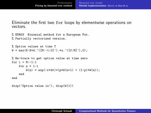
Eliminate the first two for loops by elementwise operations onvectors.
% EURO3 Binomial method for a European Put.
% Partially vectorized version.
% Option values at time T
W = max(K-S*d.^([M:-1:0]’).*u.^([0:M]’),0);
% Re-trace to get option value at time zero
for i = M:-1:1
for n = 1:i
W(n) = exp(-r*dt)*(p*W(n+1) + (1-p)*W(n));
end
end
disp(’Option value is’), disp(W(1))
Christoph Schwab Computational Methods for Quantitative Finance
PreliminariesPricing by binomial tree method
Binomial tree modelMatlab implementation: Euro1.m–Euro9.m
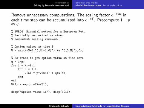
Remove unnecessary computations. The scaling factor e−r∆t ineach time step can be accumulated into e−rT . Precompute 1− pas q.
% EURO4 Binomial method for a European Put.
% Partially vectorized version.
% Redundant scaling removed.
% Option values at time T
W = max(K-S*d.^([M:-1:0]’).*u.^([0:M]’),0);
% Re-trace to get option value at time zero
q = 1-p;
for i = M:-1:1
for n = 1:i
W(n) = p*W(n+1) + q*W(n);
end
end
W(1) = exp(-r*T)*W(1);
disp(’Option value is’), disp(W(1))
Christoph Schwab Computational Methods for Quantitative Finance
PreliminariesPricing by binomial tree method
Binomial tree modelMatlab implementation: Euro1.m–Euro9.m
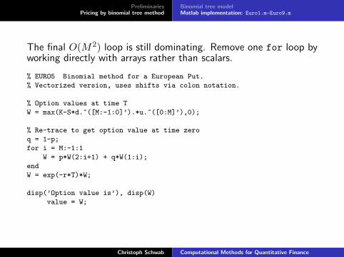
The final O(M2) loop is still dominating. Remove one for loop byworking directly with arrays rather than scalars.
% EURO5 Binomial method for a European Put.
% Vectorized version, uses shifts via colon notation.
% Option values at time T
W = max(K-S*d.^([M:-1:0]’).*u.^([0:M]’),0);
% Re-trace to get option value at time zero
q = 1-p;
for i = M:-1:1
W = p*W(2:i+1) + q*W(1:i);
end
W = exp(-r*T)*W;
disp(’Option value is’), disp(W)
value = W;
Christoph Schwab Computational Methods for Quantitative Finance
PreliminariesPricing by binomial tree method
Binomial tree modelMatlab implementation: Euro1.m–Euro9.m
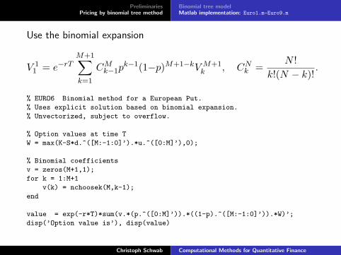
Use the binomial expansion
V 11 = e−rT
M+1∑k=1
CMk−1pk−1(1−p)M+1−kVM+1
k , CNk =N !
k!(N − k)!.
% EURO6 Binomial method for a European Put.
% Uses explicit solution based on binomial expansion.
% Unvectorized, subject to overflow.
% Option values at time T
W = max(K-S*d.^([M:-1:0]’).*u.^([0:M]’),0);
% Binomial coefficients
v = zeros(M+1,1);
for k = 1:M+1
v(k) = nchoosek(M,k-1);
end
value = exp(-r*T)*sum(v.*(p.^([0:M]’)).*((1-p).^([M:-1:0]’)).*W)’;
disp(’Option value is’), disp(value)
Christoph Schwab Computational Methods for Quantitative Finance
PreliminariesPricing by binomial tree method
Binomial tree modelMatlab implementation: Euro1.m–Euro9.m
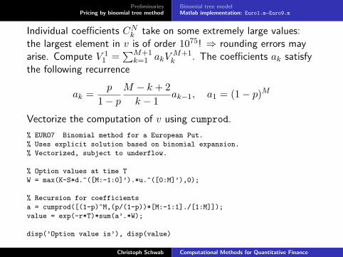
Individual coefficients CNk take on some extremely large values:the largest element in v is of order 1075! ⇒ rounding errors mayarise. Compute V 1
1 =∑M+1
k=1 akVM+1k . The coefficients ak satisfy
the following recurrence
ak =p
1− pM − k + 2k − 1
ak−1, a1 = (1− p)M
Vectorize the computation of v using cumprod.
% EURO7 Binomial method for a European Put.
% Uses explicit solution based on binomial expansion.
% Vectorized, subject to underflow.
% Option values at time T
W = max(K-S*d.^([M:-1:0]’).*u.^([0:M]’),0);
% Recursion for coefficients
a = cumprod([(1-p)^M,(p/(1-p))*[M:-1:1]./[1:M]]);
value = exp(-r*T)*sum(a’.*W);
disp(’Option value is’), disp(value)
Christoph Schwab Computational Methods for Quantitative Finance
PreliminariesPricing by binomial tree method
Binomial tree modelMatlab implementation: Euro1.m–Euro9.m
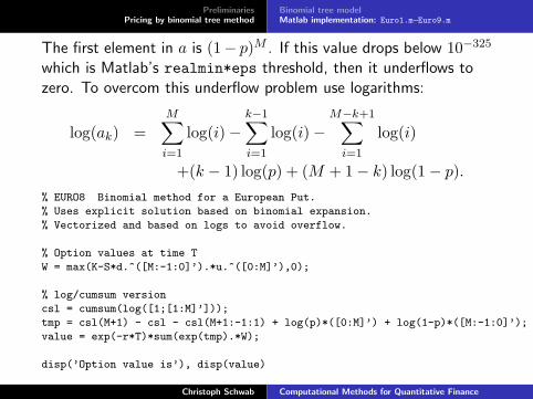
The first element in a is (1− p)M . If this value drops below 10−325
which is Matlab’s realmin*eps threshold, then it underflows tozero. To overcom this underflow problem use logarithms:
log(ak) =M∑i=1
log(i)−k−1∑i=1
log(i)−M−k+1∑i=1
log(i)
+(k − 1) log(p) + (M + 1− k) log(1− p).% EURO8 Binomial method for a European Put.
% Uses explicit solution based on binomial expansion.
% Vectorized and based on logs to avoid overflow.
% Option values at time T
W = max(K-S*d.^([M:-1:0]’).*u.^([0:M]’),0);
% log/cumsum version
csl = cumsum(log([1;[1:M]’]));
tmp = csl(M+1) - csl - csl(M+1:-1:1) + log(p)*([0:M]’) + log(1-p)*([M:-1:0]’);
value = exp(-r*T)*sum(exp(tmp).*W);
disp(’Option value is’), disp(value)
Christoph Schwab Computational Methods for Quantitative Finance
PreliminariesPricing by binomial tree method
Binomial tree modelMatlab implementation: Euro1.m–Euro9.m
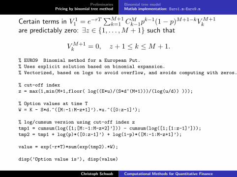
Certain terms in V 11 = e−rT
∑M+1k=1 CMk−1p
k−1(1− p)M+1−kVM+1k
are predictably zero: ∃z ∈ 1, . . . ,M + 1 such that
VM+1k = 0, z + 1 ≤ k ≤M + 1.
% EURO9 Binomial method for a European Put.
% Uses explicit solution based on binomial expansion.
% Vectorized, based on logs to avoid overflow, and avoids computing with zeros.
% cut-off index
z = max(1,min(M+1,floor( log((E*u)/(S*d^(M+1)))/(log(u/d)) )));
% Option values at time T
W = K - S*d.^([M:-1:M-z+1]’).*u.^([0:z-1]’);
% log/cumsum version using cut-off index z
tmp1 = cumsum(log([1;[M:-1:M-z+2]’])) - cumsum(log([1;[1:z-1]’]));
tmp2 = tmp1 + log(p)*([0:z-1]’) + log(1-p)*([M:-1:M-z+1]’);
value = exp(-r*T)*sum(exp(tmp2).*W);
disp(’Option value is’), disp(value)
Christoph Schwab Computational Methods for Quantitative Finance
PreliminariesPricing by binomial tree method
Binomial tree modelMatlab implementation: Euro1.m–Euro9.m
Reference:
Desmond J. Higham, Nine Ways to Implement the BinomialMethod for Option Valuation in MATLAB, SIAM Review, 2002.
(See lecture web site for the link on this paper and accompanyingMatlab files)
Christoph Schwab Computational Methods for Quantitative Finance
PreliminariesPricing by binomial tree method
Binomial tree modelMatlab implementation: Euro1.m–Euro9.m
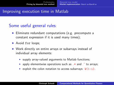
Improving execution time in Matlab
Some useful general rules:
I Eliminate redundant computations (e.g. precompute aconstant expression if it is used many times);
I Avoid for loops;
I Work directly on entire arrays or subarrays instead ofindividual array elements:
I supply array-valued arguments to Matlab functions;
I apply elementwise operations such as .* and .ˆ to arrays;
I exploit the colon notation to access subarrays: W(1:i).
Christoph Schwab Computational Methods for Quantitative Finance
Pricing by Finite Difference Solution of PDEs
Computational Methods for Quantitative FinancePricing by Finite Difference Solution of PDEs
Christoph SchwabN. Hilber, Ch. Winter
Lecture 2
Christoph Schwab Computational Methods for Quantitative Finance
Pricing by Finite Difference Solution of PDEsOption prices as solutions of PDEs: Fokker-Planck equationFinite Difference method for the heat equation
Outline
Pricing by Finite Difference Solution of PDEsOption prices as solutions of PDEs: Fokker-Planck equationFinite Difference method for the heat equation
Christoph Schwab Computational Methods for Quantitative Finance
Pricing by Finite Difference Solution of PDEsOption prices as solutions of PDEs: Fokker-Planck equationFinite Difference method for the heat equation
Setup
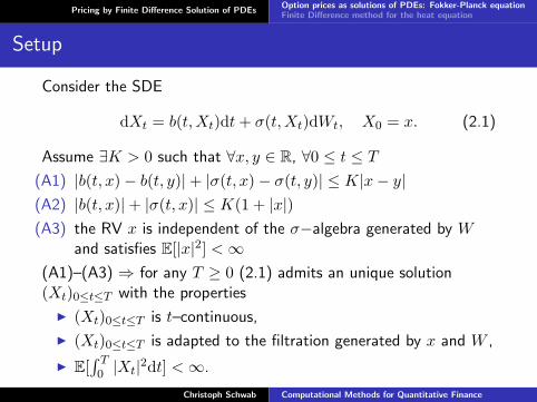
Consider the SDE
dXt = b(t,Xt)dt+ σ(t,Xt)dWt, X0 = x. (2.1)
Assume ∃K > 0 such that ∀x, y ∈ R, ∀0 ≤ t ≤ T(A1) |b(t, x)− b(t, y)|+ |σ(t, x)− σ(t, y)| ≤ K|x− y|(A2) |b(t, x)|+ |σ(t, x)| ≤ K(1 + |x|)(A3) the RV x is independent of the σ−algebra generated by W
and satisfies E[|x|2] <∞(A1)–(A3) ⇒ for any T ≥ 0 (2.1) admits an unique solution(Xt)0≤t≤T with the properties
I (Xt)0≤t≤T is t–continuous,
I (Xt)0≤t≤T is adapted to the filtration generated by x and W ,
I E[∫ T0 |Xt|2dt] <∞.
Christoph Schwab Computational Methods for Quantitative Finance
Pricing by Finite Difference Solution of PDEsOption prices as solutions of PDEs: Fokker-Planck equationFinite Difference method for the heat equation
Setup
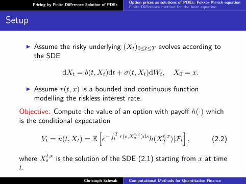
I Assume the risky underlying (Xt)0≤t≤T evolves according tothe SDE
dXt = b(t,Xt)dt+ σ(t,Xt)dWt, X0 = x.
I Assume r(t, x) is a bounded and continuous functionmodelling the riskless interest rate.
Objective: Compute the value of an option with payoff h(·) whichis the conditional expectation
Vt = u(t,Xt) = E[e−
R Tt r(s,Xt,x
s )dsh(Xt,xT )|Ft
], (2.2)
where Xt,xs is the solution of the SDE (2.1) starting from x at time
t.
Christoph Schwab Computational Methods for Quantitative Finance
Pricing by Finite Difference Solution of PDEsOption prices as solutions of PDEs: Fokker-Planck equationFinite Difference method for the heat equation
Infinitesimal generator
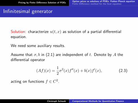
Solution: characterize u(t, x) as solution of a partial differentialequation.
We need some auxiliary results.
Assume that σ, b in (2.1) are independent of t. Denote by A thedifferential operator
(Af)(x) =12σ2(x)f ′′(x) + b(x)f ′(x), (2.3)
acting on functions f ∈ C2.
Christoph Schwab Computational Methods for Quantitative Finance
Pricing by Finite Difference Solution of PDEsOption prices as solutions of PDEs: Fokker-Planck equationFinite Difference method for the heat equation
Infinitesimal generator
Proposition
Assume that σ, b in (2.1) are independent of t. Then the process
Mt := f(Xt)−∫ t
0(Af)(Xs) ds (2.4)
is a martingale with respect to the filtration of Wt. In particular,for all t,
E[f(Xt)
]= f(x) + E
[∫ t
0Af(Xs)ds
]. (2.5)
Proof. Ito’s Lemma, stochastic integral w.r. to W is a martingale.
Christoph Schwab Computational Methods for Quantitative Finance
Pricing by Finite Difference Solution of PDEsOption prices as solutions of PDEs: Fokker-Planck equationFinite Difference method for the heat equation
Infinitesimal generator
Based on this Proposition, we have
TheoremDenote by Xx
t the solution of the SDE (2.1) with initial conditionXx
0 = x. Then for any function f ∈ C2, the functiont→ E[f(Xx
t )] is continuously differentiable and
ddt
E[f(Xx
t )]|t=0 = (Af)(x)
with A as in (2.3)
RemarkThe operator A is called infinitesimal generator of the diffusionprocess Xx
t .
Christoph Schwab Computational Methods for Quantitative Finance
Pricing by Finite Difference Solution of PDEsOption prices as solutions of PDEs: Fokker-Planck equationFinite Difference method for the heat equation
Prices of European contracts are moments of the price process Xxt
of the formu(x, t) = E
[e−
R t0 r(X
xs )dsh(Xx
t )]
(2.6)
where h(x) and r(x) are continuous functions of x ∈ R.
Such moments are solutions of deterministic PDEs, as thefollowing theorem, the so-called Feynman-Kac theorem, shows.
Christoph Schwab Computational Methods for Quantitative Finance
Pricing by Finite Difference Solution of PDEsOption prices as solutions of PDEs: Fokker-Planck equationFinite Difference method for the heat equation
Feynman-Kac
TheoremLet u(x, t) ∈ C2,1(R× R+) be a solution of the parabolic Cauchyproblem
∂tu+Au− ru = 0 in R× R+
u(x, 0) = h(x) in R (2.7)
with A as in (2.3). Then u(x, t) can be represented as in (2.6), i.e.
u(x, t) = E[e−
R t0 r(X
xs )dsh(Xx
t )].
Viceversa, any u(x, t) as in (2.6) which is in C2,1(R× R+) solvesthe deterministic Fokker Planck equation (2.7).
Christoph Schwab Computational Methods for Quantitative Finance
Pricing by Finite Difference Solution of PDEsOption prices as solutions of PDEs: Fokker-Planck equationFinite Difference method for the heat equation
This result is still true in a multi-dimensional model and for thecase when the coefficient functions b, σ and the discounting factorc depend also on t.For p ∈ N consider the system of SDEs
dXkt = bk(t,Xt)dt+
p∑j=1
σkj(t,Xt)dWjt , 1 ≤ k ≤ n. (2.8)
Denote by A the operator
(Au)(x, t) =12
tr[σσ>D2u] + 〈b,∇u〉, (2.9)
where D2 = (∂xixj )1≤i,j≤n is the Hessian, σ = (σij)1≤i≤n,1≤j≤pand 〈·, ·〉 denotes the standard inner product in Rn.
Christoph Schwab Computational Methods for Quantitative Finance
Pricing by Finite Difference Solution of PDEsOption prices as solutions of PDEs: Fokker-Planck equationFinite Difference method for the heat equation
Feynman-Kac (baskets)
Theorem(baskets)
(i) If (Xt)t≥0 is a solution of (2.8) and u(x, t) : Rn × R+ → Rhas bounded, second order derivatives in x and bounded firstorder derivatives in t and if r(t, x) : R+ × Rn → R is acontinuous, bounded function on R+ × Rn, then the process
Mt := e−R t0 r(s,Xs)dsu(Xt, t)
−∫ t
0e−
R s0 r(τ,Xτ )dτ (∂tu+Au− ru) (Xs, s)ds
is a martingale.
Christoph Schwab Computational Methods for Quantitative Finance
Pricing by Finite Difference Solution of PDEsOption prices as solutions of PDEs: Fokker-Planck equationFinite Difference method for the heat equation
(ii) Let u(x, t) ∈ C2,1(Rn × [0, T ]) be a solution of the parabolicCauchy problem
∂tu+Au− ru = 0 in Rn × R+
u(x, T ) = h(x) in Rn (2.10)
with A as in (2.9). Then u(x, t) can be represented as
u(x, t) = E[e−
R Tt r(s,Xt,x
s )dsh(Xt,xT )]. (2.11)
Christoph Schwab Computational Methods for Quantitative Finance
Pricing by Finite Difference Solution of PDEsOption prices as solutions of PDEs: Fokker-Planck equationFinite Difference method for the heat equation
Application to the Black Scholes model
Assume for simplicity that no dividends are paid.Dynamics of risky underlying: Geometric Brownian motion
dSt = St(rdt+ σdWt), S0 = S (2.12)
i.e. we have b(S) = rS, σ(S) = σS. The infinitesimal generator Ais
A =: ABS =12σ2S2∂SS + rS∂S .
Christoph Schwab Computational Methods for Quantitative Finance
Pricing by Finite Difference Solution of PDEsOption prices as solutions of PDEs: Fokker-Planck equationFinite Difference method for the heat equation
The discounted price of a European contract with payoff h(S), i.e.
V (S, t) := E[e−r(T−t)h(ST ) | St = S],
is equal to a regular solution V (S, t) of the Black Scholes (BS)equation
∂tV +ABSV − rV = 0 in R+ × [0, T )V (S, T ) = h(S) in R+
, (2.13)
where
ABS =12σ2S2∂SS + rS∂S .
Christoph Schwab Computational Methods for Quantitative Finance
Pricing by Finite Difference Solution of PDEsOption prices as solutions of PDEs: Fokker-Planck equationFinite Difference method for the heat equation
Heat equation
By change of variables
y(x, τ) := e−αx−βτV (ex, T − 2τ/σ2), α, β ∈ R
the Black-Scholes equation can be transformed to the heatequation (see exercise):
∂τy − ∂xxy = 0 in R× (0, 1/2σ2T ]y(x, 0) = y0(x) in R
We first study finite difference method on this simple example.Boundary conditions If the equation is satisfied for x ∈ (a, b), weneed conditions at x = a and x = b, for all τ . Examples:
I Dirichlet conditions: y(a, τ) = ga(τ), y(b, τ) = gb(τ).I Neumann conditions: ∂xy(a, τ) = ga(τ), ∂xy(b, τ) = gb(τ).
Remark If x ∈ R, we choose a bounded computational domain(a, b) and impose artificial boundary conditions.
Christoph Schwab Computational Methods for Quantitative Finance

Pricing by Finite Difference Solution of PDEsOption prices as solutions of PDEs: Fokker-Planck equationFinite Difference method for the heat equation
Discretization of the domain
Computational domain [a, b]× [0, τmax] is replaced by discrete grid:
(xi, τm), i = 0, . . . , N + 1, m = 0, . . . ,M,
where xi are equidistant space grid points with space step size h:
xi = a+ ih, h ≡ ∆x =b− aN + 1
,
and τm the time levels with time step size k:
τm = mk, k ≡ ∆τ =τmax
M.
Remark It is possible to use variable step sizes ∆xi and ∆τm:for example, to refine the grid near the irregularities of the solution.
Christoph Schwab Computational Methods for Quantitative Finance

Pricing by Finite Difference Solution of PDEsOption prices as solutions of PDEs: Fokker-Planck equationFinite Difference method for the heat equation
Solution on the grid
The exact solution y(x, t) is a surface on [a, b]× [0, τmax]:infinitely dimensional object.
Computer can work only with finite quantities.
Therefore, we represent the solution by its values on the grid:the surface is replaced by (N + 2)× (M + 1) points:
y(x, t) −→ ymi = y(xi, τm), i = 0, . . . , N +1, m = 0, . . . ,M.
The goal is to approximate the values ymi . Values of the solutionbetween grid points are then found by some interpolation.
Christoph Schwab Computational Methods for Quantitative Finance
Pricing by Finite Difference Solution of PDEsOption prices as solutions of PDEs: Fokker-Planck equationFinite Difference method for the heat equation
Difference Quotients (= Finite Differences)
We want to approximate the derivatives of y using only its valueson the grid. First, let us consider a function f(x) of one variable.
Assume that f is twice differentiable with continuous derivatives;we write f ∈ C2. Then, using Taylor’s formula,
f ′(x) =f(x+ h)− f(x)
h+h
2f ′′(ξ), ξ ∈ [x, x+ h] .
If fi = f(xi) are the values of f on the grid xi, we obtain
f ′(xi) ≈ fi+1 − fih
with a remainder that goes to zero as h→ 0.
Christoph Schwab Computational Methods for Quantitative Finance
Pricing by Finite Difference Solution of PDEsOption prices as solutions of PDEs: Fokker-Planck equationFinite Difference method for the heat equation
Notations
f ′(xi) =fi+1 − fi
h+O(h) =: (δ+x f)i +O(h)
f ′(xi) =fi − fi−1
h+O(h) =: (δ−x f)i +O(h)
(δ+x f)i and (δ−x f)i are called one-sided difference quotients of fwith respect to x at xi. They are accurate of first order (O(h)).
Other examples (valid for more regular functions):
f ′(xi) =fi+1 − fi−1
2h+O(h2) =: (δxf)i +O(h2) f ∈ C3 ,
f ′′(xi) =fi+1 − 2fi + fi−1
h2+O(h2) =: (δ2xxf)i +O(h2) f ∈ C4 ,
f ′(xi) =−fi+2 + 4fi+1 − 3fi
2h+O(h2) =: (δ+x f)i +O(h2) f ∈ C3 .
Christoph Schwab Computational Methods for Quantitative Finance
Pricing by Finite Difference Solution of PDEsOption prices as solutions of PDEs: Fokker-Planck equationFinite Difference method for the heat equation
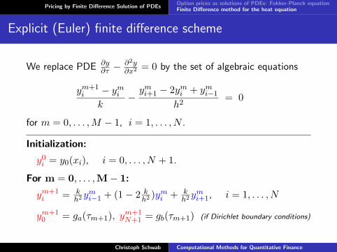
Explicit (Euler) finite difference scheme
We replace PDE ∂y∂τ − ∂2y
∂x2 = 0 by the set of algebraic equations
ym+1i − ymi
k− ymi+1 − 2ymi + ymi−1
h2= 0
for m = 0, . . . ,M − 1, i = 1, . . . , N .
Initialization:
y0i = y0(xi), i = 0, . . . , N + 1.
For m = 0, . . . ,M− 1:
ym+1i = k
h2 ymi−1 + (1− 2 k
h2 )ymi + kh2 y
mi+1, i = 1, . . . , N
ym+10 = ga(τm+1), ym+1
N+1 = gb(τm+1) (if Dirichlet boundary conditions)
Christoph Schwab Computational Methods for Quantitative Finance
Pricing by Finite Difference Solution of PDEsOption prices as solutions of PDEs: Fokker-Planck equationFinite Difference method for the heat equation
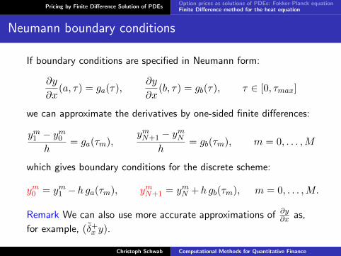
Neumann boundary conditions
If boundary conditions are specified in Neumann form:
∂y
∂x(a, τ) = ga(τ),
∂y
∂x(b, τ) = gb(τ), τ ∈ [0, τmax]
we can approximate the derivatives by one-sided finite differences:
ym1 − ym0h
= ga(τm),ymN+1 − ymN
h= gb(τm), m = 0, . . . ,M
which gives boundary conditions for the discrete scheme:
ym0 = ym1 −h ga(τm), ymN+1 = ymN +h gb(τm), m = 0, . . . ,M.
Remark We can also use more accurate approximations of ∂y∂x as,
for example, (δ+x y).
Christoph Schwab Computational Methods for Quantitative Finance
Pricing by Finite Difference Solution of PDEsOption prices as solutions of PDEs: Fokker-Planck equationFinite Difference method for the heat equation
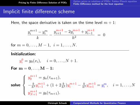
Implicit finite difference scheme
Here, the space derivative is taken on the time level m+ 1:
ym+1i − ymi
k− ym+1
i+1 − 2ym+1i + ym+1
i−1
h2= 0
for m = 0, . . . ,M − 1, i = 1, . . . , N .
Initialization:
y0i = y0(xi), i = 0, . . . , N + 1.
For m = 0, . . . ,M− 1:
solve
ym+10 = ga(τm+1),
− kh2 y
m+1i−1 + (1 + 2 k
h2 )ym+1i − k
h2 ym+1i+1 = ymi , i = 1, . . . , N
ym+1N+1 = gb(τm+1).
Christoph Schwab Computational Methods for Quantitative Finance
Pricing by Finite Difference Solution of PDEsOption prices as solutions of PDEs: Fokker-Planck equationFinite Difference method for the heat equation
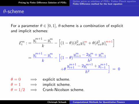
θ-scheme
For a parameter θ ∈ [0, 1], θ-scheme is a combination of explicitand implicit schemes:
Emi : =ym+1i − ymi
k−[(1− θ)(δ2xxy)mi + θ(δ2xxy)m+1
i
]=ym+1i − ymi
k−[(1− θ)y
mi+1 − 2ymi + ymi−1
h2
+θym+1i+1 − 2ym+1
i + ym+1i−1
h2
]= 0
θ = 0 =⇒ explicit scheme.θ = 1 =⇒ implicit scheme.θ = 1/2 =⇒ Crank-Nicolson scheme.
Christoph Schwab Computational Methods for Quantitative Finance
Pricing by Finite Difference Solution of PDEsOption prices as solutions of PDEs: Fokker-Planck equationFinite Difference method for the heat equation
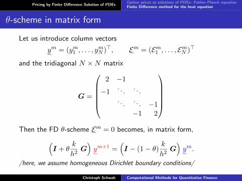
θ-scheme in matrix form
Let us introduce column vectors
ym = (ym1 , . . . , ymN )>, Em = (Em1 , . . . , EmN )>
and the tridiagonal N ×N matrix
G =
2 −1
−1. . .
. . .. . .
. . . −1−1 2
Then the FD θ-scheme Em = 0 becomes, in matrix form,(
I + θk
h2G)ym+1 =
(I − (1− θ) k
h2G)ym.
/here, we assume homogeneous Dirichlet boundary conditions/
Christoph Schwab Computational Methods for Quantitative Finance

Pricing by Finite Difference Solution of PDEsOption prices as solutions of PDEs: Fokker-Planck equationFinite Difference method for the heat equation
Notation
To shorten the notation, let us introduce matrices
B = I + θk
h2G and C = I − (1− θ) k
h2G.
The scheme becomes
Bym+1 = Cym.
To find ym+1, we have to solve this linear system:
ym+1 = B−1Cym.
Christoph Schwab Computational Methods for Quantitative Finance

Pricing by Finite Difference Solution of PDEsOption prices as solutions of PDEs: Fokker-Planck equationFinite Difference method for the heat equation
θ-scheme for some modifications of the PDE
Inhomogeneous heat equation: ∂y∂τ = ∂2y
∂x2 + f(x, τ) =⇒Bym+1 = Cym + k[θfm+1 + (1− θ)fm].
where fm = (fm1 , . . . , fmN ) and fmi = f(xi, τm).
Inhomogeneous Dirichlet BC: y(a, τ) = ga(τ), y(b, τ) = gb(τ) ⇒Bym+1 = Cym +
k
h2[θgm+1 + (1− θ)gm].
where gm =(ga(τm), 0, . . . , 0, gb(τm)
)>.
Neumann BC: ∂y∂x(a, τ) = ga(τ), ∂y
∂x(b, τ) = gb(τ) =⇒
(B−θ kh2
F )ym+1 = (C+(1− θ) kh2
F )ym+k
h[θgm+1 + (1− θ)gm].
where gm =(− ga(τm), 0, . . . , 0, gb(τm)
)>, and F contains only
two non-zero elements: F ij = 0 except F 11 = FNN = 1.
Christoph Schwab Computational Methods for Quantitative Finance
Pricing by Finite Difference Solution of PDEs
Computational Methods for Quantitative FinancePricing by Finite Difference Solution of PDEs (part 2)
Christoph SchwabN. Hilber, Ch. Winter
Lecture 3
Christoph Schwab Computational Methods for Quantitative Finance
Pricing by Finite Difference Solution of PDEsAnalysis of the Finite Difference methodFinite Difference solution of the Black-Scholes equation
Outline
Pricing by Finite Difference Solution of PDEsAnalysis of the Finite Difference methodFinite Difference solution of the Black-Scholes equation
Christoph Schwab Computational Methods for Quantitative Finance
Pricing by Finite Difference Solution of PDEsAnalysis of the Finite Difference methodFinite Difference solution of the Black-Scholes equation
Consistency of the scheme
We have replaced continuous PDE by the following FD equations:
Emi = 0, i = 1, . . . , N, m = 0, . . . ,M − 1 ,
y0i = y0(xi), i = 1, . . . , N
ym0 = 0, ymN+1 = 0, m = 0, . . . ,M (homogeneous Dirichlet BC)
DefinitionThe consistency error Emi at (xi, τm) is the difference operator Emiwith ymi replaced by y(xi, τm) where y is the exact solution.
Note Consistency error measures the quality of the approximationof the differential operator by finite differences. A scheme is calledconsistent if its consistency error goes to zero as h, k → 0.
Christoph Schwab Computational Methods for Quantitative Finance
Pricing by Finite Difference Solution of PDEsAnalysis of the Finite Difference methodFinite Difference solution of the Black-Scholes equation
Consistency error
We want to estimate the consistency errors Emi in terms of meshwidth h and time step size k.
Proposition
If the exact solution y(x, τ) of the heat equation is sufficientlysmooth, then, for m = 1, ...,M − 1 and i = 1, ..., N , we have
|Emi | ≤ C(h2 + k) 0 ≤ θ ≤ 1 ,
|Emi | ≤ C(h2 + k2) θ =12.
where C depends on the exact solution y and its derivatives.
Christoph Schwab Computational Methods for Quantitative Finance
Pricing by Finite Difference Solution of PDEsAnalysis of the Finite Difference methodFinite Difference solution of the Black-Scholes equation
Discretization error
Define εm, the error vector at time τm:
εmi = y(xi, τm)− ymi , 1 ≤ i ≤ N, 0 ≤ m ≤M .
The error vectors εmMm=0 satisfy the difference equation
1k
B εm+1 − 1k
C εm = Em
or, in explicit form,
εm+1 = Aθ εm + kB−1Em
where Aθ ≡ B−1C is called amplification matrix.
Note: the scheme is convergent (in L∞(0, τmax;L2(a, b)) norm) ifsupm
√h‖εm‖l2 → 0 as h, k → 0.
Christoph Schwab Computational Methods for Quantitative Finance
Pricing by Finite Difference Solution of PDEsAnalysis of the Finite Difference methodFinite Difference solution of the Black-Scholes equation
Recall on matrix and vector norms
Let v = (v1, . . . , vN )> and M be an N ×N matrix. We define
‖v‖`2 := (v21 + · · ·+ v2
N )1/2
‖M‖2 := supv 6=0
‖Mv‖`2‖v‖`2
.
Remark If M is symmetric with eigenvalues λl, 1 ≤ l ≤ N , then
‖M‖2 = max1≤l≤N
|λl|.
Property For all v and M , we have ‖Mv‖`2 ≤ ‖M‖2‖v‖`2 .
Remark Let f be a function on (a, b) with f(a) = f(b) = 0, andlet f = (f1, . . . , fN ) be the vector of its values on the grid. Then
‖f‖2L2(a,b) =∫ b
af2(x)dx =
N∑i=0
∫ xi+1
xi
f2(x)dx ≈N∑i=1
f2i h = h‖f‖2`2 .
Christoph Schwab Computational Methods for Quantitative Finance
Pricing by Finite Difference Solution of PDEsAnalysis of the Finite Difference methodFinite Difference solution of the Black-Scholes equation
Consistency + Stability = Convergence
Proposition
For all M ∈ N, 1 ≤ m ≤M , holds
‖εm‖`2 ≤ ‖Aθ‖m2 ‖ε0‖`2 + km−1∑n=0
‖Aθ‖m−1−n2 ‖En‖`2 .
Corollary
If the stability condition ‖Aθ‖2 ≤ 1 holds then, as M →∞,N →∞, the FD scheme converges and, if ε0 = 0,
supm‖εm‖`2 ≤ τmax sup
m‖Em‖`2 .
Christoph Schwab Computational Methods for Quantitative Finance

Pricing by Finite Difference Solution of PDEsAnalysis of the Finite Difference methodFinite Difference solution of the Black-Scholes equation
Stability
When the stability condition ‖Aθ‖2 ≤ 1 is satisfied?
We need some auxiliary results.
LemmaThe eigenvalues of the tridiagonal matrix X ∈ RN×N :
X =
α β
γ α. . .
. . .. . . βγ α
.
are given by
λX` = α+ 2
√βγ cos
( `π
N + 1
), ` = 1, . . . , N.
Christoph Schwab Computational Methods for Quantitative Finance
Pricing by Finite Difference Solution of PDEsAnalysis of the Finite Difference methodFinite Difference solution of the Black-Scholes equation
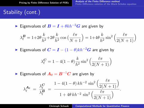
Stability (cont.)
I Eigenvalues of B = I + θkh−2G are given by
λB` = 1+2θ
k
h2+2θ
k
h2cos( `π
N + 1
)= 1+4θ
k
h2sin2
( `π
2(N + 1)
)I Eigenvalues of C = I − (1− θ)kh−2G are given by
λC` = 1− 4(1− θ) k
h2sin2
( `π
2(N + 1)
)I Eigenvalues of Aθ = B−1C are given by
λAθ` =
λC`
λB`
=1− 4(1− θ) kh−2 sin2
( `π
2(N + 1)
)1 + 4θ kh−2 sin2
( `π
2(N + 1)
) .
Christoph Schwab Computational Methods for Quantitative Finance
Pricing by Finite Difference Solution of PDEsAnalysis of the Finite Difference methodFinite Difference solution of the Black-Scholes equation
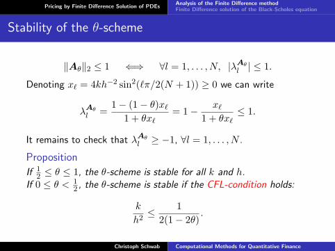
Stability of the θ-scheme
‖Aθ‖2 ≤ 1 ⇐⇒ ∀l = 1, . . . , N, |λAθl | ≤ 1.
Denoting x` = 4kh−2 sin2(`π/2(N + 1)) ≥ 0 we can write
λAθl =
1− (1− θ)x`1 + θx`
= 1− x`1 + θx`
≤ 1.
It remains to check that λAθl ≥ −1, ∀l = 1, . . . , N .
Proposition
If 12 ≤ θ ≤ 1, the θ-scheme is stable for all k and h.
If 0 ≤ θ < 12 , the θ-scheme is stable if the CFL-condition holds:
k
h2≤ 1
2(1− 2θ).
Christoph Schwab Computational Methods for Quantitative Finance
Pricing by Finite Difference Solution of PDEsAnalysis of the Finite Difference methodFinite Difference solution of the Black-Scholes equation
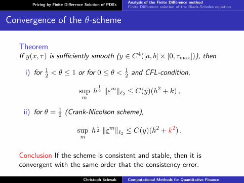
Convergence of the θ-scheme
TheoremIf y(x, τ) is sufficiently smooth (y ∈ C4([a, b]× [0, τmax])), then
i) for 12 < θ ≤ 1 or for 0 ≤ θ < 1
2 and CFL-condition,
supm
h12 ‖εm‖`2 ≤ C(y)(h2 + k) ,
ii) for θ = 12 (Crank-Nicolson scheme),
supm
h12 ‖εm‖`2 ≤ C(y)(h2 + k2) .
Conclusion If the scheme is consistent and stable, then it isconvergent with the same order that the consistency error.
Christoph Schwab Computational Methods for Quantitative Finance
Pricing by Finite Difference Solution of PDEsAnalysis of the Finite Difference methodFinite Difference solution of the Black-Scholes equation
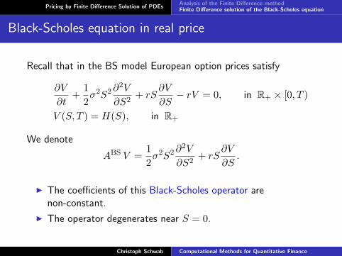
Black-Scholes equation in real price
Recall that in the BS model European option prices satisfy
∂V
∂t+
12σ2S2∂
2V
∂S2+ rS
∂V
∂S− rV = 0, in R+ × [0, T )
V (S, T ) = H(S), in R+
We denote
ABS V =12σ2S2∂
2V
∂S2+ rS
∂V
∂S.
I The coefficients of this Black-Scholes operator arenon-constant.
I The operator degenerates near S = 0.
Christoph Schwab Computational Methods for Quantitative Finance
Pricing by Finite Difference Solution of PDEsAnalysis of the Finite Difference methodFinite Difference solution of the Black-Scholes equation
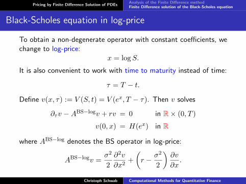
Black-Scholes equation in log-price
To obtain a non-degenerate operator with constant coefficients, wechange to log-price:
x = logS.
It is also convenient to work with time to maturity instead of time:
τ = T − t.Define v(x, τ) := V (S, t) = V (ex, T − τ). Then v solves
∂τv −ABS−logv + rv = 0 in R× (0, T )
v(0, x) = H(ex) in R
where ABS−log denotes the BS operator in log-price:
ABS−logv =σ2
2∂2v
∂x2+(r − σ2
2
)∂v
∂x.
Christoph Schwab Computational Methods for Quantitative Finance
Pricing by Finite Difference Solution of PDEsAnalysis of the Finite Difference methodFinite Difference solution of the Black-Scholes equation
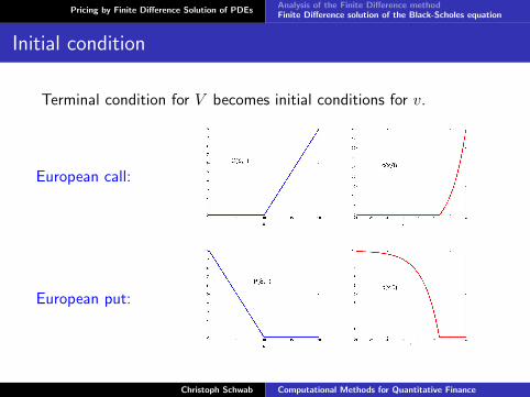
Initial condition
Terminal condition for V becomes initial conditions for v.
European call:
European put:
Christoph Schwab Computational Methods for Quantitative Finance

Pricing by Finite Difference Solution of PDEsAnalysis of the Finite Difference methodFinite Difference solution of the Black-Scholes equation
Truncation of the domain
In the European case, v(x, τ) is defined for −∞ < x <∞.
For numerical solution, we truncate the domain to (−R,R):
∂τvR −ABS−logvR + rvR = 0 in (−R,R)× (0, T ),
vR(x, 0) = H(ex) |x| < R
We then need artificial boundary conditions at x = ±R.
The simplest choice are homogeneous Dirichlet conditions:
vR(±R, τ) = 0 0 < τ < T .
Christoph Schwab Computational Methods for Quantitative Finance
Pricing by Finite Difference Solution of PDEsAnalysis of the Finite Difference methodFinite Difference solution of the Black-Scholes equation
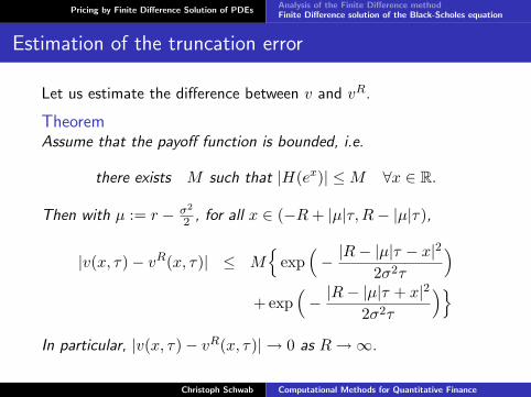
Estimation of the truncation error
Let us estimate the difference between v and vR.
TheoremAssume that the payoff function is bounded, i.e.
there exists M such that |H(ex)| ≤M ∀x ∈ R.
Then with µ := r − σ2
2 , for all x ∈ (−R+ |µ|τ,R− |µ|τ),
|v(x, τ)− vR(x, τ)| ≤ M
exp(− |R− |µ|τ − x|
2
2σ2τ
)+ exp
(− |R− |µ|τ + x|2
2σ2τ
)In particular, |v(x, τ)− vR(x, τ)| → 0 as R→∞.
Christoph Schwab Computational Methods for Quantitative Finance
Pricing by Finite Difference Solution of PDEsAnalysis of the Finite Difference methodFinite Difference solution of the Black-Scholes equation
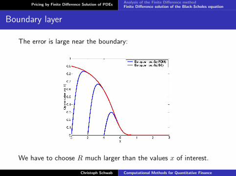
Boundary layer
The error is large near the boundary:
We have to choose R much larger than the values x of interest.
Christoph Schwab Computational Methods for Quantitative Finance
Pricing by Finite Difference Solution of PDEsAnalysis of the Finite Difference methodFinite Difference solution of the Black-Scholes equation
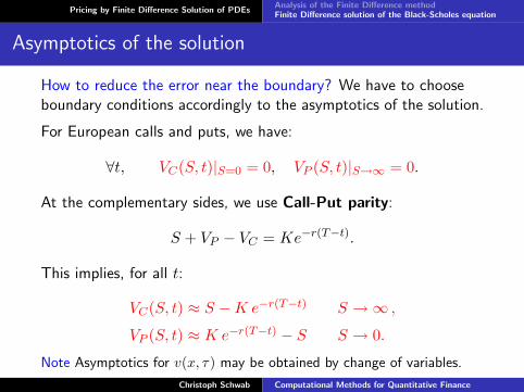
Asymptotics of the solution
How to reduce the error near the boundary? We have to chooseboundary conditions accordingly to the asymptotics of the solution.
For European calls and puts, we have:
∀t, VC(S, t)|S=0 = 0, VP (S, t)|S→∞ = 0.
At the complementary sides, we use Call-Put parity:
S + VP − VC = Ke−r(T−t).
This implies, for all t:
VC(S, t) ≈ S −K e−r(T−t) S →∞ ,
VP (S, t) ≈ K e−r(T−t) − S S → 0.
Note Asymptotics for v(x, τ) may be obtained by change of variables.
Christoph Schwab Computational Methods for Quantitative Finance
Pricing by Finite Difference Solution of PDEsAnalysis of the Finite Difference methodFinite Difference solution of the Black-Scholes equation
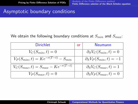
Asymptotic boundary conditions
We obtain the following boundary conditions at Smin and Smax:
Dirichlet or Neumann
VC(Smin, t) = 0 ∂SVC(Smin, t) = 0
VP (Smin, t) = Ke−r(T−t) − Smin ∂SVP (Smin, t) = −1
VC(Smax, t) = Smax −Ke−r(T−t) ∂SVC(Smax, t) = 1
VP (Smax, t) = 0 ∂SVP (Smax, t) = 0
Christoph Schwab Computational Methods for Quantitative Finance
Pricing by Finite Difference Solution of PDEsAnalysis of the Finite Difference methodFinite Difference solution of the Black-Scholes equation
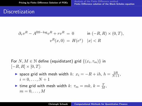
Discretization
∂τvR −ABS−logvR + rvR = 0 in (−R,R)× (0, T ),
vR(x, 0) = H(ex) |x| < R
For N,M ∈ N define (equidistant) grid (xi, τm) in[−R,R]× [0, T ]:
I space grid with mesh width h: xi = −R+ ih, h = 2RN+1 ,
i = 0, . . . , N + 1I time grid with mesh width k: τm = mk, k = T
M ,m = 0, . . . ,M
Christoph Schwab Computational Methods for Quantitative Finance
Pricing by Finite Difference Solution of PDEsAnalysis of the Finite Difference methodFinite Difference solution of the Black-Scholes equation
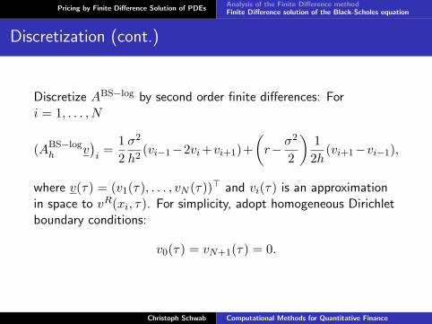
Discretization (cont.)
Discretize ABS−log by second order finite differences: Fori = 1, . . . , N
(ABS−logh v
)i=
12σ2
h2(vi−1−2vi+vi+1)+
(r− σ
2
2
)12h
(vi+1−vi−1),
where v(τ) = (v1(τ), . . . , vN (τ))> and vi(τ) is an approximationin space to vR(xi, τ). For simplicity, adopt homogeneous Dirichletboundary conditions:
v0(τ) = vN+1(τ) = 0.
Christoph Schwab Computational Methods for Quantitative Finance

Pricing by Finite Difference Solution of PDEsAnalysis of the Finite Difference methodFinite Difference solution of the Black-Scholes equation
Discretization (cont.)
Let Ah = ABS−logh − rI ∈ RN×N . Then (where ˙= ∂τ )
v = Ahv, v(0) = H(ex),
where x = (x1, . . . , xN )>.
This is a N ×N -system of ordinary differential equations.
To discretize it, use the θ-scheme. Let wm be an approximation tov(τm). We obtain
1k(wm+1 − wm) = Ah(θwm+1 + (1− θ)wm).
Christoph Schwab Computational Methods for Quantitative Finance
Pricing by Finite Difference Solution of PDEsAnalysis of the Finite Difference methodFinite Difference solution of the Black-Scholes equation
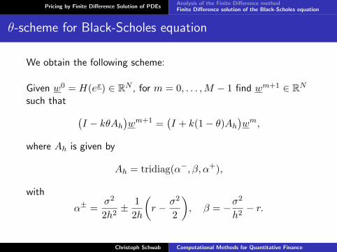
θ-scheme for Black-Scholes equation
We obtain the following scheme:
Given w0 = H(ex) ∈ RN , for m = 0, . . . ,M − 1 find wm+1 ∈ RN
such that (I − kθAh
)wm+1 =
(I + k(1− θ)Ah
)wm,
where Ah is given by
Ah = tridiag(α−, β, α+),
with
α± =σ2
2h2± 1
2h
(r − σ2
2
), β = −σ
2
h2− r.
Christoph Schwab Computational Methods for Quantitative Finance
Pricing by Finite Difference Solution of PDEsAnalysis of the Finite Difference methodFinite Difference solution of the Black-Scholes equation
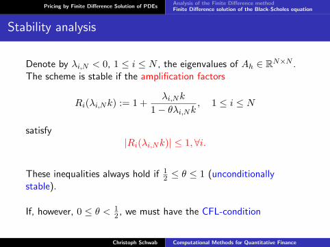
Stability analysis
Denote by λi,N < 0, 1 ≤ i ≤ N , the eigenvalues of Ah ∈ RN×N .The scheme is stable if the amplification factors
Ri(λi,Nk) := 1 +λi,Nk
1− θλi,Nk , 1 ≤ i ≤ N
satisfy|Ri(λi,Nk)| ≤ 1,∀i.
These inequalities always hold if 12 ≤ θ ≤ 1 (unconditionally
stable).
If, however, 0 ≤ θ < 12 , we must have the CFL-condition
Christoph Schwab Computational Methods for Quantitative Finance
Pricing by Finite Difference Solution of PDEsAnalysis of the Finite Difference methodFinite Difference solution of the Black-Scholes equation
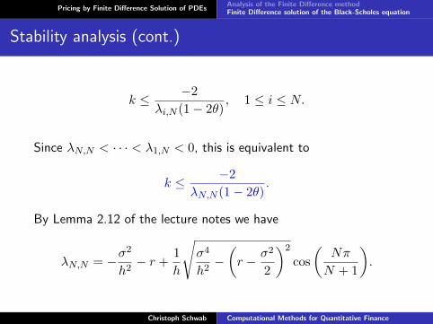
Stability analysis (cont.)
k ≤ −2λi,N (1− 2θ)
, 1 ≤ i ≤ N.
Since λN,N < · · · < λ1,N < 0, this is equivalent to
k ≤ −2λN,N (1− 2θ)
.
By Lemma 2.12 of the lecture notes we have
λN,N = −σ2
h2− r +
1h
√σ4
h2−(r − σ2
2
)2
cos(
Nπ
N + 1
).
Christoph Schwab Computational Methods for Quantitative Finance
Pricing by Finite Difference Solution of PDEsAnalysis of the Finite Difference methodFinite Difference solution of the Black-Scholes equation
Stability analysis (cont.)
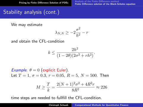
We may estimate
λN,N ≥ −2σ2
h2− r
and obtain the CFL-condition
k ≤ 2h2
(1− 2θ)(2σ2 + rh2).
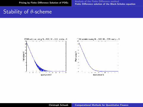
Example. θ = 0 (explicit Euler).Let T = 1, σ = 0.3, r = 0.05, R = 5, N = 500. Then
M ≥ T
k=
2(N + 1)2σ2 + 4R2r
8R2≈ 226
time steps are needed to fullfill the CFL-condition.
Christoph Schwab Computational Methods for Quantitative Finance
Pricing by Finite Difference Solution of PDEsAnalysis of the Finite Difference methodFinite Difference solution of the Black-Scholes equation
Stability of θ-scheme
Christoph Schwab Computational Methods for Quantitative Finance
Pricing by Finite Difference Solution of PDEsAnalysis of the Finite Difference methodFinite Difference solution of the Black-Scholes equation
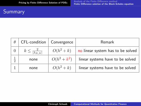
Summary
θ CFL-condition Convergence Remark
0 k ≤ 2|λN,N | O(h2 + k) no linear system has to be solved
12 none O(h2 + k2) linear systems have to be solved
1 none O(h2 + k) linear systems have to be solved
Christoph Schwab Computational Methods for Quantitative Finance
Pricing American options using Finite Difference method
Computational Methods for Quantitative FinancePricing American options using Finite Difference method
Christoph SchwabN. Hilber, Ch. Winter
Lecture 4
Christoph Schwab Computational Methods for Quantitative Finance
Pricing American options using Finite Difference method
Black-Scholes Variational InequalityDomain truncationFinite Difference discretizationSolution of matrix linear complementarity problems (LCPs)
Outline
Pricing American options using Finite Difference methodBlack-Scholes Variational InequalityDomain truncationFinite Difference discretizationSolution of matrix linear complementarity problems (LCPs)
Christoph Schwab Computational Methods for Quantitative Finance
Pricing American options using Finite Difference method
Black-Scholes Variational InequalityDomain truncationFinite Difference discretizationSolution of matrix linear complementarity problems (LCPs)
Assumption
Black-Scholes market, no dividends (δ = 0):
dSt = St(rdt+ σ dWt) t > 0 .
American options are options that can be exercised at any time upto the expiration date T . The problem of optimal exercising isequivalent to an optimal stopping problem: denote by Tt,T the setof all stopping times with values in the interval (t, T ). Then, withthe payoff H(S) = (S −K)+ (call) or H(S) = (K − S)+ (put),
V am(S, t) = supτ∈Tt,T
E[e−r(τ−t)H(Se(r−
σ2
2)(τ−t)+σ(Wτ−Wt))
].
Christoph Schwab Computational Methods for Quantitative Finance
Pricing American options using Finite Difference method
Black-Scholes Variational InequalityDomain truncationFinite Difference discretizationSolution of matrix linear complementarity problems (LCPs)
Basic properties of the Value V am(S, t) of an American contract(δ = 0):
V amC = V eur
C
V amP ≥ V eur
P
V amP (S, t) ≥ (K − S)+, V am
C (S, t) ≥ (S −K)+ .
As for the European vanilla, there is a close connection betweenthe probabilistic representation of the option’s value and adeterministic, PDE based representation of this value.
Christoph Schwab Computational Methods for Quantitative Finance
Pricing American options using Finite Difference method
Black-Scholes Variational InequalityDomain truncationFinite Difference discretizationSolution of matrix linear complementarity problems (LCPs)
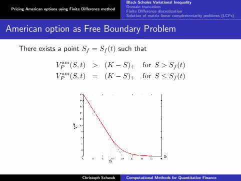
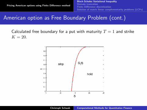
American option as Free Boundary Problem
There exists a point Sf = Sf (t) such that
V amP (S, t) > (K − S)+ for S > Sf (t)V amP (S, t) = (K − S)+ for S ≤ Sf (t)
Christoph Schwab Computational Methods for Quantitative Finance
Pricing American options using Finite Difference method
Black-Scholes Variational InequalityDomain truncationFinite Difference discretizationSolution of matrix linear complementarity problems (LCPs)
American option as Free Boundary Problem (cont.)
A priori the boundary Sf (t) is not known. Therefore, the problemof calculating V am
P (S, t) for S > Sf (t) is called freeboundary-value problem and Sf (t) is called free boundary.
The free boundary Sf (t) separates R+ × [0, T ] into thecontinuation region (hold the option) and the stopping region(exercise the option).
As soon the price of the asset reaches Sf (t) the holder shouldexercise the option. The corresponding time instant τ is calledstopping time.
Christoph Schwab Computational Methods for Quantitative Finance
Pricing American options using Finite Difference method
Black-Scholes Variational InequalityDomain truncationFinite Difference discretizationSolution of matrix linear complementarity problems (LCPs)
American option as Free Boundary Problem (cont.)
Calculated free boundary for a put with maturity T = 1 and strikeK = 20.
Christoph Schwab Computational Methods for Quantitative Finance
Pricing American options using Finite Difference method
Black-Scholes Variational InequalityDomain truncationFinite Difference discretizationSolution of matrix linear complementarity problems (LCPs)
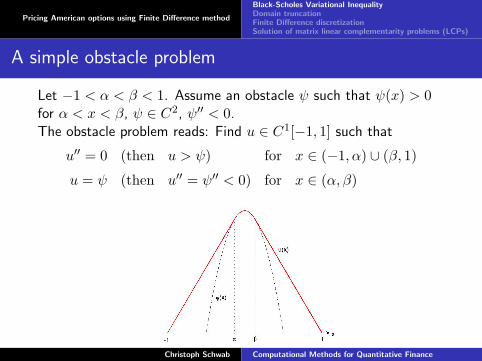
A simple obstacle problem
Let −1 < α < β < 1. Assume an obstacle ψ such that ψ(x) > 0for α < x < β, ψ ∈ C2, ψ′′ < 0.The obstacle problem reads: Find u ∈ C1[−1, 1] such that
u′′ = 0 (then u > ψ) for x ∈ (−1, α) ∪ (β, 1)
u = ψ (then u′′ = ψ′′ < 0) for x ∈ (α, β)
Christoph Schwab Computational Methods for Quantitative Finance
Pricing American options using Finite Difference method
Black-Scholes Variational InequalityDomain truncationFinite Difference discretizationSolution of matrix linear complementarity problems (LCPs)
A simple obstacle problem (cont.)
This manifests a complementarity in the sense
if u > ψ, then u′′ = 0if u = ψ, then u′′ < 0
The obstacle problem can be reformulated as: Find u ∈ C1[−1, 1]such that u(±1) = 0 and such that
−u′′ ≥ 0 in (−1, 1)u ≥ ψ in (−1, 1)
u′′(u− ψ) = 0 in (−1, 1)
Christoph Schwab Computational Methods for Quantitative Finance
Pricing American options using Finite Difference method
Black-Scholes Variational InequalityDomain truncationFinite Difference discretizationSolution of matrix linear complementarity problems (LCPs)
Linear complementarity problem (LCP)
The finite difference discretization of the obstacle problemproceeds in the usual fashion:
−1 = x0 < x1 < . . . < xi < . . . < xN < xN+1 = 1
with
xi = −1 + i∆x, i = 0, 1, . . . , N + 1 , ∆x = 2/(N + 1),
yi ≈ u(xi) : y = (y1, . . . , yN )> ∈ RN .
Christoph Schwab Computational Methods for Quantitative Finance
Pricing American options using Finite Difference method
Black-Scholes Variational InequalityDomain truncationFinite Difference discretizationSolution of matrix linear complementarity problems (LCPs)
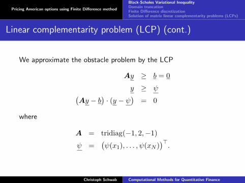
Linear complementarity problem (LCP) (cont.)
We approximate the obstacle problem by the LCP
Ay ≥ b = 0
y ≥ ψ(Ay − b) · (y − ψ) = 0
where
A = tridiag(−1, 2,−1)
ψ =(ψ(x1), . . . , ψ(xN )
)>.
Christoph Schwab Computational Methods for Quantitative Finance
Pricing American options using Finite Difference method
Black-Scholes Variational InequalityDomain truncationFinite Difference discretizationSolution of matrix linear complementarity problems (LCPs)
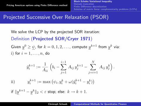
Projected Successive Over Relaxation (PSOR)
We solve the LCP by the projected SOR iteration:
Definition (Projected SOR/Cryer 1971)
Given y0 ≥ ψ, for k = 0, 1, 2, . . . , compute yk+1 from yk via:
i) for i = 1, . . . , n, do
yk+1i :=
1Aii
(bi −
i−1∑j=1
Aij yk+1j −
N∑j=i+1
Aij ykj
).
ii) yk+1i := max
(ψi, y
ki + ω(yk+1
i − yki ))
if ‖yk+1 − yk‖2 < ε stop; else: k → k + 1.
Christoph Schwab Computational Methods for Quantitative Finance
Pricing American options using Finite Difference method
Black-Scholes Variational InequalityDomain truncationFinite Difference discretizationSolution of matrix linear complementarity problems (LCPs)
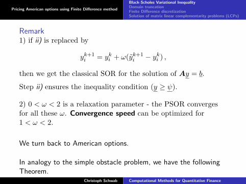
Remark1) if ii) is replaced by
yk+1i = yki + ω(yk+1
i − yki ) ,
then we get the classical SOR for the solution of Ay = b.
Step ii) ensures the inequality condition (y ≥ ψ).
2) 0 < ω < 2 is a relaxation parameter - the PSOR convergesfor all these ω. Convergence speed can be optimized for1 < ω < 2.
We turn back to American options.
In analogy to the simple obstacle problem, we have the followingTheorem.
Christoph Schwab Computational Methods for Quantitative Finance
Pricing American options using Finite Difference method
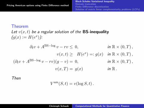
Black-Scholes Variational InequalityDomain truncationFinite Difference discretizationSolution of matrix linear complementarity problems (LCPs)
TheoremLet v(x, t) be a regular solution of the BS-inequality(g(x) := H(ex)):
∂tv +ABS−log v − rv ≤ 0, in R× (0, T ) ,
v(x, t) ≥ H(ex) =: g(x) in R× (0, T ) ,
(∂tv +ABS−log v − rv)(g − v) = 0, in R× (0, T ) ,
v(x, T ) = g(x) in R .
ThenV am(S, t) = v(logS, t) .
Christoph Schwab Computational Methods for Quantitative Finance
Pricing American options using Finite Difference method
Black-Scholes Variational InequalityDomain truncationFinite Difference discretizationSolution of matrix linear complementarity problems (LCPs)
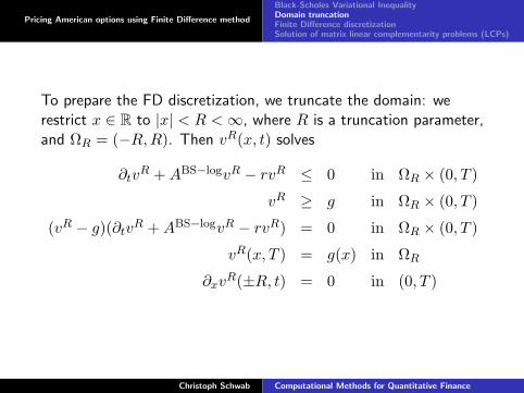
To prepare the FD discretization, we truncate the domain: werestrict x ∈ R to |x| < R <∞, where R is a truncation parameter,and ΩR = (−R,R). Then vR(x, t) solves
∂tvR +ABS−logvR − rvR ≤ 0 in ΩR × (0, T )
vR ≥ g in ΩR × (0, T )
(vR − g)(∂tvR +ABS−logvR − rvR) = 0 in ΩR × (0, T )
vR(x, T ) = g(x) in ΩR
∂xvR(±R, t) = 0 in (0, T )
Christoph Schwab Computational Methods for Quantitative Finance
Pricing American options using Finite Difference method
Black-Scholes Variational InequalityDomain truncationFinite Difference discretizationSolution of matrix linear complementarity problems (LCPs)
As in the European case, we choose the time step ∆t = k = TM ,
and the space step ∆x = h = 2RN+1 .
Then
tm = mk, xi = −R+ ih, i = 0, . . . , N + 1, k = 0, . . . ,M.
The vector of approximate option prices at time level m is
w = (w1, . . . , wN )>; we expect that w(m)i ∼ v(xi, tm).
Christoph Schwab Computational Methods for Quantitative Finance
Pricing American options using Finite Difference method
Black-Scholes Variational InequalityDomain truncationFinite Difference discretizationSolution of matrix linear complementarity problems (LCPs)
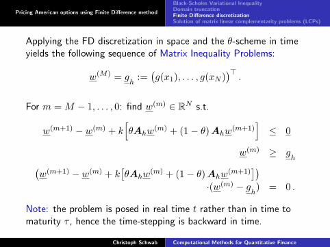
Applying the FD discretization in space and the θ-scheme in timeyields the following sequence of Matrix Inequality Problems:
w(M) = gh
:=(g(x1), . . . , g(xN )
)>.
For m = M − 1, . . . , 0: find w(m) ∈ RN s.t.
w(m+1) − w(m) + k[θAhw
(m) + (1− θ) Ahw(m+1)
]≤ 0
w(m) ≥ gh(
w(m+1) − w(m) + k[θAhw
(m) + (1− θ) Ahw(m+1)
])·(w(m) − g
h) = 0 .
Note: the problem is posed in real time t rather than in time tomaturity τ , hence the time-stepping is backward in time.
Christoph Schwab Computational Methods for Quantitative Finance
Pricing American options using Finite Difference method
Black-Scholes Variational InequalityDomain truncationFinite Difference discretizationSolution of matrix linear complementarity problems (LCPs)
Here, as in the European case
Ah := ABS−logh − rI,
where, due to homogeneous Neumann boundary conditions
0 = ∂xvR(±R, t)
=1
2h(± 3vR(±R, t)∓ 4vR(±R∓ h)± vR(±R∓ 2h, t)
)+O(h2)
the tridiagonal matrix ABS−logh ∈ RN×N is given by
Christoph Schwab Computational Methods for Quantitative Finance
Pricing American options using Finite Difference method
Black-Scholes Variational InequalityDomain truncationFinite Difference discretizationSolution of matrix linear complementarity problems (LCPs)
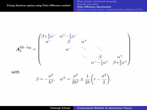
ABS−logh =
β+4
3α− α+−1
3α−
α− β α+
α−. . .
. . .. . . β α+
α−−13α
+ β+43α
+
with
β = −σ2
h2, α± =
σ2
2h2± 1
2h
(r − σ2
2
).
Christoph Schwab Computational Methods for Quantitative Finance
Pricing American options using Finite Difference method
Black-Scholes Variational InequalityDomain truncationFinite Difference discretizationSolution of matrix linear complementarity problems (LCPs)
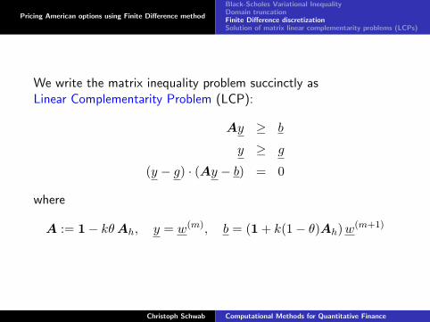
We write the matrix inequality problem succinctly asLinear Complementarity Problem (LCP):
Ay ≥ b
y ≥ g
(y − g) · (Ay − b) = 0
where
A := 1− kθAh, y = w(m), b = (1 + k(1− θ)Ah)w(m+1)
Christoph Schwab Computational Methods for Quantitative Finance
Pricing American options using Finite Difference method
Black-Scholes Variational InequalityDomain truncationFinite Difference discretizationSolution of matrix linear complementarity problems (LCPs)
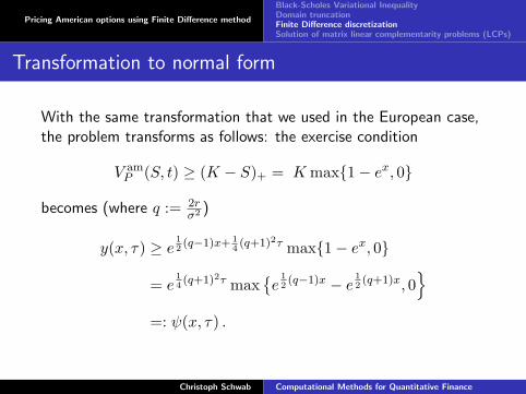
Transformation to normal form
With the same transformation that we used in the European case,the problem transforms as follows: the exercise condition
V amP (S, t) ≥ (K − S)+ = K max1− ex, 0
becomes (where q := 2rσ2 )
y(x, τ) ≥ e 12(q−1)x+ 1
4(q+1)2τ max1− ex, 0
= e14(q+1)2τ max
e
12(q−1)x − e 1
2(q+1)x, 0
=: ψ(x, τ) .
Christoph Schwab Computational Methods for Quantitative Finance
Pricing American options using Finite Difference method
Black-Scholes Variational InequalityDomain truncationFinite Difference discretizationSolution of matrix linear complementarity problems (LCPs)
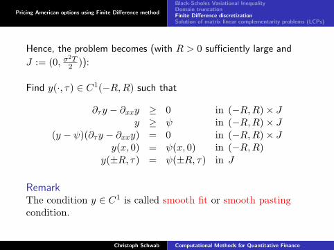
Hence, the problem becomes (with R > 0 sufficiently large and
J := (0, σ2T2 )):
Find y(·, τ) ∈ C1(−R,R) such that
∂τy − ∂xxy ≥ 0 in (−R,R)× Jy ≥ ψ in (−R,R)× J
(y − ψ)(∂τy − ∂xxy) = 0 in (−R,R)× Jy(x, 0) = ψ(x, 0) in (−R,R)
y(±R, τ) = ψ(±R, τ) in J
RemarkThe condition y ∈ C1 is called smooth fit or smooth pastingcondition.
Christoph Schwab Computational Methods for Quantitative Finance

Pricing American options using Finite Difference method
Black-Scholes Variational InequalityDomain truncationFinite Difference discretizationSolution of matrix linear complementarity problems (LCPs)
Inserting finite differences in the parabolic variational inequality(assumed to hold pointwise), we get at each time level the linearsystem of algebraic inequalities for the unknown values
y(m)i ≈ y(xi, τm) at the nodes (xi, τm):
y(m+1)i −λθ(y(m+1)
i+1 − 2y(m+1)i + y
(m+1)i−1
)− y
(m)i −λ(1− θ)(y(m)
i+1 − 2y(m)i + y
(m)i−1
) ≥ 0,
with
λ :=∆t
∆x2=
k
h2.
Christoph Schwab Computational Methods for Quantitative Finance
Pricing American options using Finite Difference method
Black-Scholes Variational InequalityDomain truncationFinite Difference discretizationSolution of matrix linear complementarity problems (LCPs)
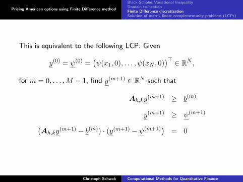
This is equivalent to the following LCP: Given
y(0) = ψ(0) =(ψ(x1, 0), . . . , ψ(xN , 0)
)> ∈ RN ,
for m = 0, . . . ,M − 1, find y(m+1) ∈ RN such that
Ah,ky(m+1) ≥ b(m)
y(m+1) ≥ ψ(m+1)(Ah,ky
(m+1) − b(m)) · (y(m+1) − ψ(m+1))
= 0
Christoph Schwab Computational Methods for Quantitative Finance
Pricing American options using Finite Difference method
Black-Scholes Variational InequalityDomain truncationFinite Difference discretizationSolution of matrix linear complementarity problems (LCPs)
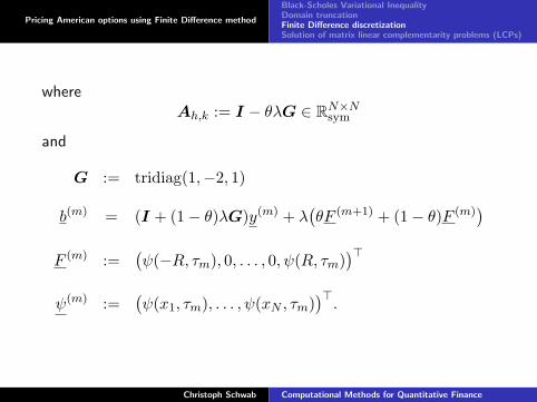
whereAh,k := I − θλG ∈ RN×N
sym
and
G := tridiag(1,−2, 1)
b(m) = (I + (1− θ)λG)y(m) + λ(θF (m+1) + (1− θ)F (m)
)F (m) :=
(ψ(−R, τm), 0, . . . , 0, ψ(R, τm)
)>ψ(m) :=
(ψ(x1, τm), . . . , ψ(xN , τm)
)>.
Christoph Schwab Computational Methods for Quantitative Finance
Pricing American options using Finite Difference method
Black-Scholes Variational InequalityDomain truncationFinite Difference discretizationSolution of matrix linear complementarity problems (LCPs)
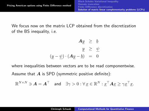
We focus now on the matrix LCP obtained from the discretizationof the BS inequality, i.e.
Ay ≥ b
y ≥ ψ
(y − ψ) · (Ay − b) = 0
where inequalities between vectors are to be read componentwise.
Assume that A is SPD (symmetric positive definite):
RN×N 3 A = A> and ∃γ > 0 : ∀x ∈ RN : x>Ax ≥ γx>x.
Christoph Schwab Computational Methods for Quantitative Finance
Pricing American options using Finite Difference method
Black-Scholes Variational InequalityDomain truncationFinite Difference discretizationSolution of matrix linear complementarity problems (LCPs)
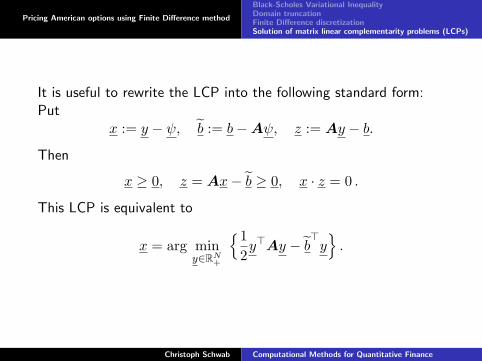
It is useful to rewrite the LCP into the following standard form:Put
x := y − ψ, b := b−Aψ, z := Ay − b.Then
x ≥ 0, z = Ax− b ≥ 0, x · z = 0 .
This LCP is equivalent to
x = arg miny∈RN+
12y>Ay − b>y
.
Christoph Schwab Computational Methods for Quantitative Finance
Pricing American options using Finite Difference method
Black-Scholes Variational InequalityDomain truncationFinite Difference discretizationSolution of matrix linear complementarity problems (LCPs)
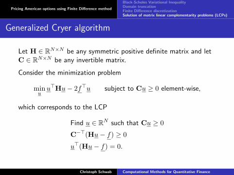
Generalized Cryer algorithm
Let H ∈ RN×N be any symmetric positive definite matrix and letC ∈ RN×N be any invertible matrix.
Consider the minimization problem
minuu>Hu− 2f>u subject to Cu ≥ 0 element-wise,
which corresponds to the LCP
Find u ∈ RN such that Cu ≥ 0
C−>(Hu− f) ≥ 0
u>(Hu− f) = 0.
Christoph Schwab Computational Methods for Quantitative Finance
Pricing American options using Finite Difference method
Black-Scholes Variational InequalityDomain truncationFinite Difference discretizationSolution of matrix linear complementarity problems (LCPs)
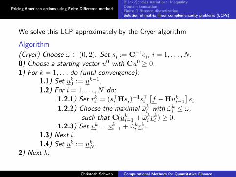
We solve this LCP approximately by the Cryer algorithm
Algorithm
(Cryer) Choose ω ∈ (0, 2). Set si := C−1ei, i = 1, . . . , N .0) Choose a starting vector u0 with Cu0 ≥ 0.1) For k = 1, . . . do (until convergence):
1.1) Set uk0 := uk−1.1.2) For i = 1, . . . , N do:
1.2.1) Set rki = (s>i Hsi)−1s>i[f −Huki−1
]si.
1.2.2) Choose the maximal ωki with ωki ≤ ω,such that C(uki−1 + ωki r
ki ) ≥ 0.
1.2.3) Set uki = uki−1 + ωki rki .
1.3) Next i.1.4) Set uk := ukN .
2) Next k.
Christoph Schwab Computational Methods for Quantitative Finance
Pricing American options using Finite Difference method
Black-Scholes Variational InequalityDomain truncationFinite Difference discretizationSolution of matrix linear complementarity problems (LCPs)
TheoremUnder the above assumptions, the Generalized Cryer Algorithmconverges to the solution of the minimization problem.
Christoph Schwab Computational Methods for Quantitative Finance
Pricing barrier and Asian contracts by Finite Difference method
Computational Methods for Quantitative FinanceFinite Difference methods for barrier and Asian contracts
Prof. Ch. SchwabN. Hilber, Ch. Winter
Lecture 5
Christoph Schwab Computational Methods for Quantitative Finance

Pricing barrier and Asian contracts by Finite Difference methodBarrier OptionsAsian OptionsMatlab implementation
Outline
Pricing barrier and Asian contracts by Finite Difference methodBarrier OptionsAsian OptionsMatlab implementation
Christoph Schwab Computational Methods for Quantitative Finance
Pricing barrier and Asian contracts by Finite Difference methodBarrier OptionsAsian OptionsMatlab implementation
Barrier options differ from vanillas in the sense that the optioncontract is triggered if the price of the underlying hits some barrier,S = B, say, during [0, T ].
To be more specific, consider a contract which pays a specifiedamount at maturity T provided during 0 ≤ t ≤ T the price St doesnot cross a specified barrier B > 0 either from above (‘down-and-out’ barrier option) or from below (‘up-and-out’ barrieroption).
If the barrier is crossed before T , the option expires worthless(‘out’ barrier option). We assume here for convenience that B isconstant.
Christoph Schwab Computational Methods for Quantitative Finance
Pricing barrier and Asian contracts by Finite Difference methodBarrier OptionsAsian OptionsMatlab implementation
The 4 standard ‘out’ barrier options on a risky asset are
1. down-and-out call with terminal payoff (ST −K)+ with valueV Cdo(K,B, T ;S, t) at spot price S and time t,
2. down-and-out put with terminal payoff (K − ST )+ and withvalue V P
do(K,B, T ;S, t),
3. up-and-out put with terminal payoff (K − ST )+ and withvalue V P
uo(K,B, T ;S, t),
4. up-and-out call with terminal payoff (ST −K)+ and withvalue V C
uo(K,B, T ;S, t).
An “in” barrier option becomes the corresponding European vanillawhen the barrier B is crossed at time t ∈ (0, T ). E.g., theup-and-in call becomes the European call when B is crossed frombelow; we denote its price at spot S and time t byV Cui (K,B, T ;S, t).
Christoph Schwab Computational Methods for Quantitative Finance
Pricing barrier and Asian contracts by Finite Difference methodBarrier OptionsAsian OptionsMatlab implementation
A European plain vanilla option pays the same at T as adown-and-out plus an up-and-in with the same barrier B and ofthe same type (call/put) as the plain vanilla. The standard noarbitrage consideration shows that pricing an “in” barrier reducesto pricing the corresponding “out” barrier contract and a plainEuropean vanilla, i.e.
V Cdi (K,B, T ;S, t) = V C(K,T ;S, t)− V C
do(K,B, T ;S, t)
V Cui (K,B, T ;S, t) = V C(K,T ;S, t)− V C
uo(K,B, T ;S, t).(5.1)
Analogous identities hold for values of the other barrier contracts,too.
Christoph Schwab Computational Methods for Quantitative Finance
Pricing barrier and Asian contracts by Finite Difference methodBarrier OptionsAsian OptionsMatlab implementation
Out-Barrier
Assume that the riskless rate r > 0 is independent of t. Inlog-price x = logS, g(x) = (ex −K)+ = f(ex) is the terminalpayoff of a down-and-out call with barrier B = 1 for convenience(general B will be dealt with below). Let
v(x, t) = V Cdo(K, 1, T ;S, t)|x=logS
be the price of the down-and-out barrier call at t < T and at spotS > B = 1. Then,
v(x, t) = E[er(t−T )g(XT )1τ0>T|Xt = x
]where τ0 is the hitting time of (−∞, 0] = (−∞, logB] by theprocess Xt.
Christoph Schwab Computational Methods for Quantitative Finance
Pricing barrier and Asian contracts by Finite Difference methodBarrier OptionsAsian OptionsMatlab implementation
Consequently, v(x, t) is the solution of the BS equation in log-price
∂tv +ABS−logv − rv = 0 in (0,∞)× (0, T )v(0, t) = 0 in (0, T )v(x, T ) = g(x) in (0,∞)
In real price S and for a general barrier B > 0,V (S, t) = V C
do(K,B, T ;S, t) satisfies
V Cdo(K,B, T ;S, t) = E
[er(t−T )f(ST )1τB>T|St = S
]where τB is the first hitting time of [0, B] by the process St.
Christoph Schwab Computational Methods for Quantitative Finance
Pricing barrier and Asian contracts by Finite Difference methodBarrier OptionsAsian OptionsMatlab implementation
Therefore, V (S, t) = V Cdo(K,B, T ;S, t) is solution of the
deterministic BS equation
∂tV +ABSV − rV = 0 in (B,∞)× (0, T )V (B, t) = 0 in (0, T )V (S, T ) = f(S) in (B,∞)
(5.2)
As St →∞, the probability that St ≤ B gets small, so we expectfor 0 < t < T that
V (S, t) ∼ S as S →∞ . (5.3)
The above equations specify V (S, t) completely, and can be solvedapproximately with the FD methods of the previous sections.
Christoph Schwab Computational Methods for Quantitative Finance
Pricing barrier and Asian contracts by Finite Difference methodBarrier OptionsAsian OptionsMatlab implementation
In-Barriers
“In”-barriers become worthless unless St reaches B before T . If Stcrosses B before T , then the barrier option becomes a plain vanillawith identical payoff.
To derive the BS equations for “in” barrier contracts, we considera down-and-in European call and denote by C(S, t) a Europeanvanilla call with same K,T as the ‘down-and-in’ barrier call.
Since the BS equations are linear, we apply the principle ofsuperposition and use (5.1) to derive the BS equations for the “in”barrier.
Christoph Schwab Computational Methods for Quantitative Finance
Pricing barrier and Asian contracts by Finite Difference methodBarrier OptionsAsian OptionsMatlab implementation
We get for V (S, t) = V Cdi (K,B, T ;S, t) the BS PDE
∂tV +ABSV − rV = 0 (B,∞)× (0, T ),
and, by (5.1) and (5.3)
V (S, t)→ 0 as S →∞ .
Finally, again by (5.1) and superposition, we get the terminalcondition
V (S, T ) = 0 in (B,∞)
If S(t) = B for some t < T , then V Cdo(B, t) = 0 yields in (5.1)
V (B, t) = C(B, t) .
Therefore, we must only solve BS (5.2) for S > B.
Christoph Schwab Computational Methods for Quantitative Finance
Pricing barrier and Asian contracts by Finite Difference methodBarrier OptionsAsian OptionsMatlab implementation
European Average Strikes
Asians are path-dependent: their payoffs depend on price history.Consider a European contract with payoff depending on S and on
T∫0
ϕ(S(τ), τ)dτ,
where ϕ is a given function of S, t. E.g. an average strike call haspayoff function
f(S, T ) =
(S − 1
T
∫ T
0S(τ)dτ
)+
.
Christoph Schwab Computational Methods for Quantitative Finance
Pricing barrier and Asian contracts by Finite Difference methodBarrier OptionsAsian OptionsMatlab implementation
To get the PDE for Asians, we introduce the new variable
I(t) :=
t∫0
ϕ(S(τ), τ)dτ . (5.4)
Since the history of the asset price is independent of the currentprice we may treat S(t), I(t) and t as independent variables. Thevalue of an Asian will then be searched in the form V (S, I, t). Toderive a PDE for V , we need a SDE for I(t). Formally, for smalldt > 0,
I(t+ dt) = I + dI =
t+dt∫0
ϕ(S(τ), τ)dτ
=
t∫0
ϕ(S(τ), τ)dτ + ϕ(S(t), t)dt+O(dt) ,
Christoph Schwab Computational Methods for Quantitative Finance
Pricing barrier and Asian contracts by Finite Difference methodBarrier OptionsAsian OptionsMatlab implementation
hence, as dt→ 0, we get the deterministic equation:
dI = ϕ(S, t)dt .
Note that the vector process (S(t), I(t)) is a diffusion. In fact, forϕ(S, t) = S
dS(t) = r S(t)dt+ σ S(t) dWt ,
dI(t) = S(t)dt .
The infinitesimal generator AAS of this diffusion is given by
AASV =σ2
2S2∂2
SS V + r S∂SV + ϕ(S, t)∂IV.
Christoph Schwab Computational Methods for Quantitative Finance
Pricing barrier and Asian contracts by Finite Difference methodBarrier OptionsAsian OptionsMatlab implementation
Applying Ito’s lemma to V (S, I, t) gives the relation
dV = σS∂SV dW +(σ2
2S2∂2
SSV +rS∂SV +∂tV +ϕ(S, t)∂IV)
dt .
No-arbitrage arguments lead to the following PDE for V (S, I, t):
LASV := ∂tV+ϕ(S, t)∂IV+σ2
2S2∂2
SSV+rS∂SV−rV = 0 . (5.5)
The terminal condition is, for the average strike,
V (S, I, T ) = (S − I/T )+ =: f(S, I) ;
the boundary conditions in S are as for the BS case.
Christoph Schwab Computational Methods for Quantitative Finance
Pricing barrier and Asian contracts by Finite Difference methodBarrier OptionsAsian OptionsMatlab implementation
American Average Strikes
Denoting by LAS the operator in (5.5), we find for the value ofAmerican-Asian style contracts the parabolic differential inequality:
LAS V ≤ 0
and the constraint
V (S, I, t) ≥ f(S, I, t) = (S − I/t)+ , 0 < t < T
for the American average strike call. Also, the complementaritycondition
(V − f) · LAS V = 0
must hold, and we have the final condition
V (S, I, T ) = f(S, I, T ) .
The above equations/inequalities specify the value of the Americanaverage strike call.
Christoph Schwab Computational Methods for Quantitative Finance
Pricing barrier and Asian contracts by Finite Difference methodBarrier OptionsAsian OptionsMatlab implementation
Similarity Reduction
In many cases, the bivariate PDE (5.5) can be reduced to aunivariate one the numerical solution of which is less costly. Forillustration, consider the average strike European call:
LAS V = 0, V (S, I, T ) = (S − I/T )+, I(t) =
t∫0
S(τ)dτ .
Writing
f(S, I, T ) = (S − I/T )+ = Smax(
1− 1ST
T∫0
S(τ)dτ, 0),
Christoph Schwab Computational Methods for Quantitative Finance

Pricing barrier and Asian contracts by Finite Difference methodBarrier OptionsAsian OptionsMatlab implementation
and changing the variables
R :=1S
t∫0
S(τ)dτ =I
S,
we get the pay-off Smax(1−R/T, 0).
Making the Ansatz V (S, I, t) = SH(R, t), we find from LASV = 0that H must satisfy the PDE
∂tH +σ2
2R2∂2
RRH + (1− rR)∂RH = 0, 0 < t < T (5.6)
with terminal condition
H(R, T ) = (1−R/T )+ .
Christoph Schwab Computational Methods for Quantitative Finance
Pricing barrier and Asian contracts by Finite Difference methodBarrier OptionsAsian OptionsMatlab implementation
For the boundary conditions at R = 0, R→∞, we get (exercise)
∂tH + ∂RH = 0 at R = 0, 0 < t < T ,
H(R, t) = 0 as R→∞ .
Christoph Schwab Computational Methods for Quantitative Finance
Pricing barrier and Asian contracts by Finite Difference methodBarrier OptionsAsian OptionsMatlab implementation
FD Discretization
We solve (5.6) by Finite-Difference time-stepping from T = M∆tto t = 0, with ∆t = T/M , and truncate 0 ≤ R <∞ to0 ≤ R ≤ Rmax = N∆R.
Let tm = m∆t, Rn = n∆R, m = M, . . . , 0, n = 0, . . . , N . We useFinite Differences with Hm
n ∼ H(Rn, tm). Recall (for f ∈ C4, withfn := f(xn)):
f ′(xn) =1h
(fn+1 − fn
)+O(h) := (δxf)n +O(h)
f ′(xn) =1
2h(− fn+2 + 4fn+1 − 3fn
)+O(h2) := (δ+x f)n +O(h2)
f ′′(xn) =1h2
(fn+1 − 2fn − fn−2
)+O(h2) := (δ2xxf)n +O(h2)
Christoph Schwab Computational Methods for Quantitative Finance
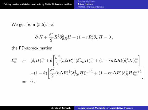
Pricing barrier and Asian contracts by Finite Difference methodBarrier OptionsAsian OptionsMatlab implementation
We get from (5.6), i.e.
∂tH +σ2
2R2∂2
RRH + (1− rR)∂RH = 0 ,
the FD-approximation
Emn := (δtH)mn + θ
[σ2
2(n∆R)2(δ2RRH)mn + (1− rn∆R)(δ+RH)mn
]+(1− θ)
[σ2
2(n∆R)2(δ2RRH)m+1
n + (1− rn∆R)(δ+RH)m+1n
]= 0 .
Christoph Schwab Computational Methods for Quantitative Finance
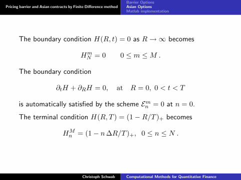
Pricing barrier and Asian contracts by Finite Difference methodBarrier OptionsAsian OptionsMatlab implementation
The boundary condition H(R, t) = 0 as R→∞ becomes
HmN = 0 0 ≤ m ≤M .
The boundary condition
∂tH + ∂RH = 0, at R = 0, 0 < t < T
is automatically satisfied by the scheme Emn = 0 at n = 0.
The terminal condition H(R, T ) = (1−R/T )+ becomes
HMn = (1− n∆R/T )+, 0 ≤ n ≤ N .
Christoph Schwab Computational Methods for Quantitative Finance
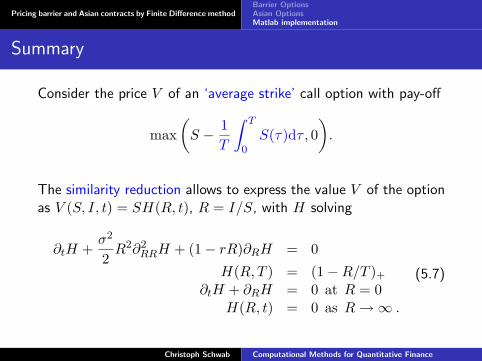
Pricing barrier and Asian contracts by Finite Difference methodBarrier OptionsAsian OptionsMatlab implementation
Summary
Consider the price V of an ‘average strike’ call option with pay-off
max(S − 1
T
∫ T
0S(τ)dτ , 0
).
The similarity reduction allows to express the value V of the optionas V (S, I, t) = SH(R, t), R = I/S, with H solving
∂tH +σ2
2R2∂2
RRH + (1− rR)∂RH = 0
H(R, T ) = (1−R/T )+∂tH + ∂RH = 0 at R = 0
H(R, t) = 0 as R→∞ .
(5.7)
Christoph Schwab Computational Methods for Quantitative Finance
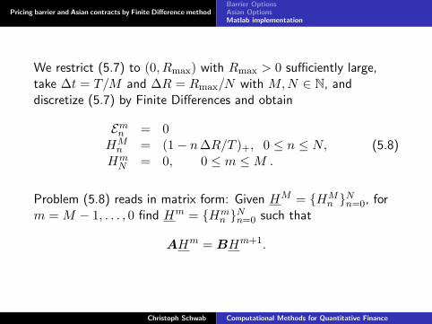
Pricing barrier and Asian contracts by Finite Difference methodBarrier OptionsAsian OptionsMatlab implementation
We restrict (5.7) to (0, Rmax) with Rmax > 0 sufficiently large,take ∆t = T/M and ∆R = Rmax/N with M,N ∈ N, anddiscretize (5.7) by Finite Differences and obtain
Emn = 0HMn = (1− n∆R/T )+, 0 ≤ n ≤ N,
HmN = 0, 0 ≤ m ≤M .
(5.8)
Problem (5.8) reads in matrix form: Given HM = HMn Nn=0, for
m = M − 1, . . . , 0 find Hm = Hmn Nn=0 such that
AHm = BHm+1.
Christoph Schwab Computational Methods for Quantitative Finance
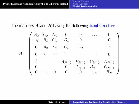
Pricing barrier and Asian contracts by Finite Difference methodBarrier OptionsAsian OptionsMatlab implementation
The matrices A and B having the following band structure
A =
B0 C0 D0 0 0 . . . 0A1 B1 C1 D1 0 0
0 A2 B2 C2 D2...
0 0. . .
. . .. . .
. . . 0... AN−2 BN−2 CN−2 DN−2
0 0 AN−1 BN−1 CN−1
0 . . . 0 0 0 AN BN
Christoph Schwab Computational Methods for Quantitative Finance
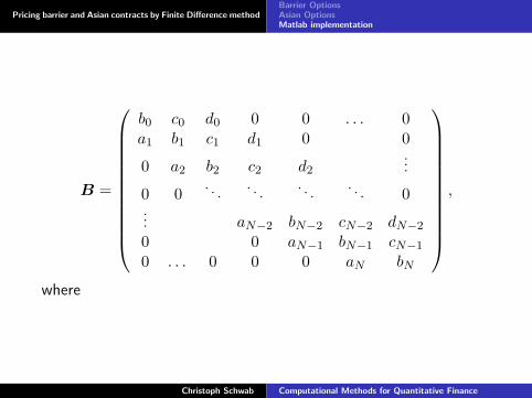
Pricing barrier and Asian contracts by Finite Difference methodBarrier OptionsAsian OptionsMatlab implementation
B =
b0 c0 d0 0 0 . . . 0a1 b1 c1 d1 0 0
0 a2 b2 c2 d2...
0 0. . .
. . .. . .
. . . 0... aN−2 bN−2 cN−2 dN−2
0 0 aN−1 bN−1 cN−1
0 . . . 0 0 0 aN bN
,
where
Christoph Schwab Computational Methods for Quantitative Finance
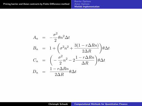
Pricing barrier and Asian contracts by Finite Difference methodBarrier OptionsAsian OptionsMatlab implementation
An = −σ2
2θn2∆t
Bn = 1 +(σ2n2 +
3(1− r∆Rn)2∆R
)θ∆t
Cn =(− σ2
2n2 − 2
1− r∆Rn∆R
)θ∆t
Dn =1− r∆Rn
2∆Rθ∆t
Christoph Schwab Computational Methods for Quantitative Finance
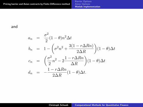
Pricing barrier and Asian contracts by Finite Difference methodBarrier OptionsAsian OptionsMatlab implementation
and
an =σ2
2(1− θ)n2∆t
bn = 1−(σ2n2 +
3(1− r∆Rn)2∆R
)(1− θ)∆t
cn =(σ2
2n2 − 2
1− r∆Rn∆R
)(1− θ)∆t
dn = −1− r∆Rn2∆R
(1− θ)∆t.
Christoph Schwab Computational Methods for Quantitative Finance
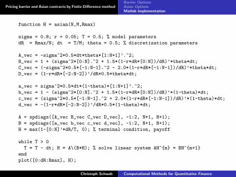
Pricing barrier and Asian contracts by Finite Difference methodBarrier OptionsAsian OptionsMatlab implementation
function H = asian(N,M,Rmax)
sigma = 0.8; r = 0.05; T = 0.5; % model parameters
dR = Rmax/N; dt = T/M; theta = 0.5; % discretization parameters
A_vec = -sigma^2*0.5*dt*theta*[1:N+1]’.^2;
B_vec = 1 + (sigma^2*[0:N].^2 + 1.5*(1-r*dR*[0:N])/dR)’*theta*dt;
C_vec = (-sigma^2*0.5*[-1:N-1].^2 - 2.0*(1-r*dR*[-1:N-1])/dR)’*theta*dt;
D_vec = (1-r*dR*[-2:N-2])’/dR*0.5*theta*dt;
a_vec = sigma^2*0.5*dt*(1-theta)*[1:N+1]’.^2;
b_vec = 1 - (sigma^2*[0:N].^2 + 1.5*(1-r*dR*[0:N])/dR)’*(1-theta)*dt;
c_vec = (sigma^2*0.5*[-1:N-1].^2 + 2.0*(1-r*dR*[-1:N-1])/dR)’*(1-theta)*dt;
d_vec = -(1-r*dR*[-2:N-2])’/dR*0.5*(1-theta)*dt;
A = spdiags([A_vec B_vec C_vec D_vec], -1:2, N+1, N+1);
B = spdiags([a_vec b_vec c_vec d_vec], -1:2, N+1, N+1);
H = max(1-[0:N]’*dR/T, 0); % terminal condition, payoff
while T > 0
T = T - dt; H = A\(B*H); % solve linear system AH^m = BH^m+1
end
plot([0:dR:Rmax], H);
Christoph Schwab Computational Methods for Quantitative Finance
The idea of finite element methodsVariational formulation of parabolic problems
Computational Methods for Quantitative FinancePricing by Finite Element Methods
Prof. Ch. SchwabN. Hilber, Ch. Winter
Lecture 6
Christoph Schwab Computational Methods for Quantitative Finance

The idea of finite element methodsVariational formulation of parabolic problems
Variational formulationGalerkin discretization
Outline
The idea of finite element methodsVariational formulationGalerkin discretization
Variational formulation of parabolic problemsGeneral frameworkExamples
Christoph Schwab Computational Methods for Quantitative Finance

The idea of finite element methodsVariational formulation of parabolic problems
Variational formulationGalerkin discretization
Problem to solve: (here, A is a linear differential operator)
∂u
∂t−Au = f in (0, T )× Iu(x, 0) = u0(x) in I
Multiply by a test function v(x) and integrate on I: Denote(u, v) :=
∫I uv and a(u, v) := −(Au, v) (bilinear form).
Variational formulation: Find u ∈ L2(0, T ;V ) ∩H1(0, T ;V ∗) suchthat
ddt
(u(t), v) + a(u(t), v) = (f(t), v) in (0, T ), ∀ v ∈ V ,u(0) = u0,
where V is some space of test functions.
Christoph Schwab Computational Methods for Quantitative Finance
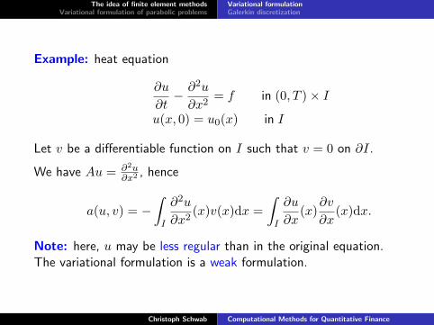
The idea of finite element methodsVariational formulation of parabolic problems
Variational formulationGalerkin discretization
Example: heat equation
∂u
∂t− ∂2u
∂x2= f in (0, T )× I
u(x, 0) = u0(x) in I
Let v be a differentiable function on I such that v = 0 on ∂I.
We have Au = ∂2u∂x2 , hence
a(u, v) = −∫I
∂2u
∂x2(x)v(x)dx =
∫I
∂u
∂x(x)
∂v
∂x(x)dx.
Note: here, u may be less regular than in the original equation.The variational formulation is a weak formulation.
Christoph Schwab Computational Methods for Quantitative Finance
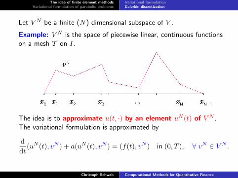
The idea of finite element methodsVariational formulation of parabolic problems
Variational formulationGalerkin discretization
Let V N be a finite (N) dimensional subspace of V .
Example: V N is the space of piecewise linear, continuous functionson a mesh T on I.
The idea is to approximate u(t, ·) by an element uN (t) of V N .The variational formulation is approximated by
ddt
(uN (t), vN ) + a(uN (t), vN ) = (f(t), vN ) in (0, T ), ∀ vN ∈ V N .
Christoph Schwab Computational Methods for Quantitative Finance
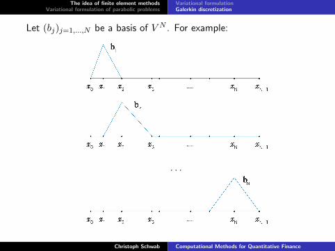
The idea of finite element methodsVariational formulation of parabolic problems
Variational formulationGalerkin discretization
Let (bj)j=1,...,N be a basis of V N . For example:
. . .
Christoph Schwab Computational Methods for Quantitative Finance
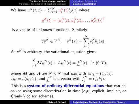
The idea of finite element methodsVariational formulation of parabolic problems
Variational formulationGalerkin discretization
We have uN (t, x) =∑N
j=1 uNj (t)bj(x) where
uN (t) = (uN1 (t), uN2 (t), . . . , uNN (t))>
is a vector of unknown functions. Similarly,
∀vN ∈ V N , vN (x) =N∑j=1
vNj bj(x).
As vN is arbitrary, the variational equation gives
ddt
MuN (t) + AuN (t) = fN (t) in (0, T ),
where M and A are N ×N matrices with Mij = (bi, bj),Aij = a(bj , bi), and fN is a vector with fNj = (f, bj).
This is a system of ordinary differential equations that can besolved using some discretization in time (e.g., explicit, implicit, orCrank-Nicolson scheme).
Christoph Schwab Computational Methods for Quantitative Finance

The idea of finite element methodsVariational formulation of parabolic problems
General frameworkExamples
Outline
The idea of finite element methodsVariational formulationGalerkin discretization
Variational formulation of parabolic problemsGeneral frameworkExamples
Christoph Schwab Computational Methods for Quantitative Finance
The idea of finite element methodsVariational formulation of parabolic problems
General frameworkExamples
Recall that we consider the following problem:
∂u
∂t−Au = f in (0, T )× I
u(x, 0) = u0(x) in I
and its variational formulation:
ddt
(u(t), v) + a(u(t), v) = (f(t), v) in (0, T ), ∀ v ∈ V ,u(0) = u0.
I What are the conditions on the operator A, initial condition u0,right-hand side f , and the space of test functions V for thisproblem to have a unique solution?
I What is the regularity of this solution?
The answers are given in a general framework of Hilbert spaces.
Christoph Schwab Computational Methods for Quantitative Finance

The idea of finite element methodsVariational formulation of parabolic problems
General frameworkExamples
Recall on Hilbert spaces
• Hilbert space: vector space H with scalar (= inner) product (u, v).Example: H = L2(I), (u, v) =
∫I u(x)v(x)dx.
• If X is a vector space, X∗ denotes the space of continuous linearfunctionals on X (dual space):
f ∈ X∗ is a continuous linear mapping from X to R.
If x ∈ X and f ∈ X∗, we denote f(x) = 〈f, x〉 (dual pairing).
• If H is a Hilbert space, H∗ may be identified with H:
f ∈ H∗ ⇐⇒ ∃ l ∈ H : ∀x ∈ H, 〈f, x〉 = (l, x).
We identify f with l and write H ∼= H∗.
Christoph Schwab Computational Methods for Quantitative Finance
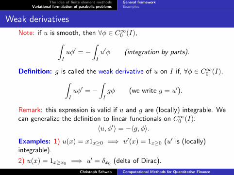
The idea of finite element methodsVariational formulation of parabolic problems
General frameworkExamples
Weak derivatives
Note: if u is smooth, then ∀φ ∈ C∞0 (I),∫Iuφ′ = −
∫Iu′φ (integration by parts).
Definition: g is called the weak derivative of u on I if, ∀φ ∈ C∞0 (I),∫Iuφ′ = −
∫Igφ (we write g = u′).
Remark: this expression is valid if u and g are (locally) integrable. Wecan generalize the definition to linear functionals on C∞0 (I):
〈u, φ′〉 = −〈g, φ〉.Examples: 1) u(x) = x1x≥0 =⇒ u′(x) = 1x≥0 (u′ is (locally)integrable).
2) u(x) = 1x≥x0 =⇒ u′ = δx0 (delta of Dirac).
Christoph Schwab Computational Methods for Quantitative Finance

The idea of finite element methodsVariational formulation of parabolic problems
General frameworkExamples
Recall on Sobolev spaces
The weak derivatives always exist but are not always integrable.
Definition: W 1,2(I) ≡ H1(I) is the space of square integrablefunctions with square integrable first derivative:
H1(I) =u ∈ L2(I) such that u′ ∈ L2(I)
Note: more generally, we can define spaces Wn,p(I) of functions withn weak derivatives, all in Lp(I) (integrable with power p).
Remark: H1(I) is a Hilbert space with the following scalar product:
(u, v) =∫Iuv +
∫Iu′v′.
Christoph Schwab Computational Methods for Quantitative Finance
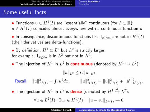
The idea of finite element methodsVariational formulation of parabolic problems
General frameworkExamples
Some useful facts
• Functions u ∈ H1(I) are “essentially” continuous (for I ⊂ R):u ∈ H1(I) coincides almost everywhere with a continuous function u.
• In consequence, discontinuous functions like 1x≥x0 are not in H1(I)(their derivatives are delta-functions).
• By definition, H1 ⊂ L2 but L2 is strictly larger:for example, 1x≥x0 is in L2 but not in H1.
• The injection of H1 in L2 is continuous (denoted by H1 → L2):
‖u‖L2 ≤ C‖u‖H1
Recall: ‖u‖2L2(I) =∫I u
2dx, ‖u‖2H1(I) = ‖u‖2L2(I) + ‖u′‖2L2(I) .
• The injection of H1 in L2 is dense (denoted by H1 d→ L2):
∀u ∈ L2(I), ∃vn ∈ H1(I) : ‖u− vn‖L2(I) → 0.
Christoph Schwab Computational Methods for Quantitative Finance
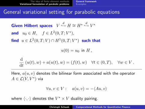
The idea of finite element methodsVariational formulation of parabolic problems
General frameworkExamples
General variational setting for parabolic equations
Given Hilbert spaces Vd→ H ∼= H∗
d→ V ∗
and u0 ∈ H, f ∈ L2(0, T ;V ∗),
find u ∈ L2(0, T ;V ) ∩H1(0, T ;V ∗) such that
u(0) = u0 in H ,
ddt
(u(t), w) + a(u(t), w) = (f(t), w) ∀t ∈ (0, T ), ∀w ∈ V .
Here, a(u, v) denotes the bilinear form associated with the operatorA ∈ L(V, V ∗) via
∀u, v ∈ V : a(u, v) = −〈Au, v〉
where 〈·, ·〉 denotes the V ∗ × V duality pairing.
Christoph Schwab Computational Methods for Quantitative Finance
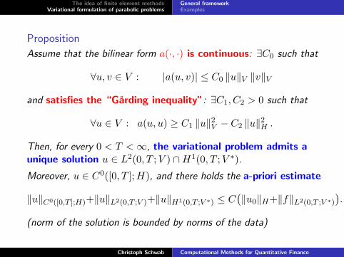
The idea of finite element methodsVariational formulation of parabolic problems
General frameworkExamples
Proposition
Assume that the bilinear form a(·, ·) is continuous: ∃C0 such that
∀u, v ∈ V : |a(u, v)| ≤ C0 ‖u‖V ‖v‖Vand satisfies the “Garding inequality”: ∃C1, C2 > 0 such that
∀u ∈ V : a(u, u) ≥ C1 ‖u‖2V − C2 ‖u‖2H .
Then, for every 0 < T <∞, the variational problem admits aunique solution u ∈ L2(0, T ;V ) ∩H1(0, T ;V ∗).
Moreover, u ∈ C0([0, T ];H), and there holds the a-priori estimate
‖u‖C0([0,T ];H)+‖u‖L2(0,T ;V )+‖u‖H1(0,T ;V ∗) ≤ C(‖u0‖H+‖f‖L2(0,T ;V ∗)
).
(norm of the solution is bounded by norms of the data)
Christoph Schwab Computational Methods for Quantitative Finance
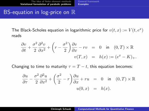
The idea of finite element methodsVariational formulation of parabolic problems
General frameworkExamples
BS-equation in log-price on R
The Black-Scholes equation in logarithmic price for v(t, x) := V (t, ex)reads
∂v
∂t+σ2
2∂2v
∂x2+(r − σ2
2
)∂v
∂x− rv = 0 in (0, T )× R
v(T, x) = h(x) := (ex −K)+.
Changing to time to maturity τ = T − t, this equation becomes:
∂u
∂τ− σ2
2∂2u
∂x2+(σ2
2− r)∂u
∂x+ ru = 0 in (0, T )× R
u(0, x) = h(x).
Christoph Schwab Computational Methods for Quantitative Finance

The idea of finite element methodsVariational formulation of parabolic problems
General frameworkExamples
If h ∈ L2(R) then this problem fits into the general framework with
I H = L2(R)I V = H1(R)I u0 = h
I f = 0I and the bilinear form:
a(u, v) =σ2
2
∫R
u′(x)v′(x)dx+(σ2
2− r)∫
R
u′(x)v(x)dx+∫R
ru(x)v(x)dx.
It can be shown that a(·, ·) is continuous and satisfies the Gardinginequality. In consequence, the general existence result applies.
Christoph Schwab Computational Methods for Quantitative Finance
The idea of finite element methodsVariational formulation of parabolic problems
General frameworkExamples
For most payoffs, h is not in L2(R). In the case of call options,h grows exponentially at infinity: h(x) = (ex −K)+.
To deal with such payoffs, we introduce weighted Sobolev spaces.
We define H1ν (R) (ν ∈ R) by
H1ν (R) := v ∈ L1
loc(R) | veν|x|, v′eν|x| ∈ L2(R).
Similarly,L2ν(R) := v ∈ L1
loc(R) | veν|x| ∈ L2(R).
Note: with this notation, the payoff function of a call belongs toH1−µ(R) for any µ > 1.
• L2ν(R) is a Hilbert space with scalar product
(u, v) =∫
Ru(x)v(x)e2ν|x|dx.
Christoph Schwab Computational Methods for Quantitative Finance
The idea of finite element methodsVariational formulation of parabolic problems
General frameworkExamples
For the variational formulation of this problem, we choose:
I H = L2−µ(R), V = H1−µ(R), u0 = h, f = 0,
I and the bilinear form:
aBS−log−µ (u, v) =
σ2
2
∫R
u′(x)v′(x)e−2µ|x| dx
+∫R
ru(x)v(x)e−2µ|x| dx
+∫R
(− µσ2sign(x) +
(σ2
2− r))
u′(x)v(x)e−2µ|x| dx.
Again, it can be shown that aBS−log−µ (·, ·) is continuous and satisfies the
Garding inequality. So, there exists a unique solution
u ∈ L2((0, T );H1−µ(R)) ∩H1((0, T );H1
−µ(R)∗).
Christoph Schwab Computational Methods for Quantitative Finance
The idea of finite element methodsVariational formulation of parabolic problems
General frameworkExamples
Localization. Excess to payoff
We localize the equation to a bounded computational domainΩR = (−R,R). This requires artificial boundary conditions at ±R.
To choose good conditions, we analyze the solution at infinity.
More precisely, we prove that the excess to payoff
U := u− e−rth(x+ rt)
decays exponentially at infinity.
Christoph Schwab Computational Methods for Quantitative Finance
The idea of finite element methodsVariational formulation of parabolic problems
General frameworkExamples
Assume that h ∈ H1−ν(R) with ν > 0 (in particular, h is continuous).Remark: satisfied for puts and calls (but not for binary options).
Substituting u(τ, x) = U(τ, x) + e−rτh(x+ rτ) into the equation,we observe that U solves the following variational problem:
find U ∈ L2((0, T );H1ν (R)) ∩H1((0, T );H1
ν (R)∗) s.t. ∀ v ∈ H1ν (R)(
dUdτ
(τ, ·), v)L2ν(R)
+ aBS−logν (U(τ, ·), v) = e−rτ
σ2
2K〈f(τ, ·), ve2ν|x|〉
U(0, ·) = 0 in L2ν(R)
where we denote by 〈·, ·〉 the(H1ν (R)
)∗ ×H1ν (R) duality pairing.
Note: H = L2ν(R), V = H1
ν (R), u0 = 0, and, in the case of a call,
f = e−rτ σ2
2 Kδln(K)−rτ .
Corollary: excess to payoff U decays exponentially at infinity.In consequence, zero boundary conditions are a good choice for U .
Christoph Schwab Computational Methods for Quantitative Finance
The idea of finite element methodsVariational formulation of parabolic problems
General frameworkExamples
Space H10(I)H10(I)H10(I)
For localized problems and barrier contracts, we needfunctional spaces with boundary conditions.
Definition
W 1,20 (I) ≡ H1
0 (I) = C10 (I) ‖·‖H1(I)
(closure of C10 (I) with respect to the norm of H1(I)).
Proposition
u ∈ H1(I) belongs to H10 (I) if and only if u = 0 on ∂I.
Christoph Schwab Computational Methods for Quantitative Finance
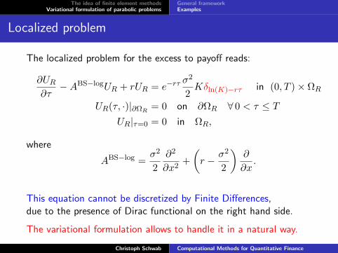
The idea of finite element methodsVariational formulation of parabolic problems
General frameworkExamples
Localized problem
The localized problem for the excess to payoff reads:
∂UR∂τ−ABS−logUR + rUR = e−rτ
σ2
2Kδln(K)−rτ in (0, T )× ΩR
UR(τ, ·)|∂ΩR = 0 on ∂ΩR ∀ 0 < τ ≤ TUR|τ=0 = 0 in ΩR,
where
ABS−log =σ2
2∂2
∂x2+(r − σ2
2
)∂
∂x.
This equation cannot be discretized by Finite Differences,due to the presence of Dirac functional on the right hand side.
The variational formulation allows to handle it in a natural way.
Christoph Schwab Computational Methods for Quantitative Finance
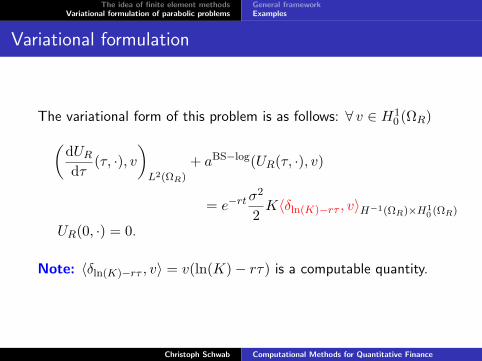
The idea of finite element methodsVariational formulation of parabolic problems
General frameworkExamples
Variational formulation
The variational form of this problem is as follows: ∀ v ∈ H10 (ΩR)(
dURdτ
(τ, ·), v)L2(ΩR)
+ aBS−log(UR(τ, ·), v)
= e−rtσ2
2K〈δln(K)−rτ , v〉H−1(ΩR)×H1
0 (ΩR)
UR(0, ·) = 0.
Note: 〈δln(K)−rτ , v〉 = v(ln(K)− rτ) is a computable quantity.
Christoph Schwab Computational Methods for Quantitative Finance
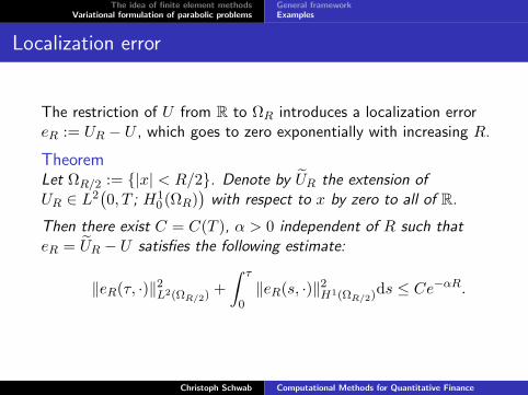
The idea of finite element methodsVariational formulation of parabolic problems
General frameworkExamples
Localization error
The restriction of U from R to ΩR introduces a localization erroreR := UR − U , which goes to zero exponentially with increasing R.
TheoremLet ΩR/2 := |x| < R/2. Denote by UR the extension ofUR ∈ L2
(0, T ; H1
0 (ΩR))
with respect to x by zero to all of R.
Then there exist C = C(T ), α > 0 independent of R such thateR = UR − U satisfies the following estimate:
‖eR(τ, ·)‖2L2(ΩR/2) +∫ τ
0‖eR(s, ·)‖2H1(ΩR/2)ds ≤ Ce−αR.
Christoph Schwab Computational Methods for Quantitative Finance
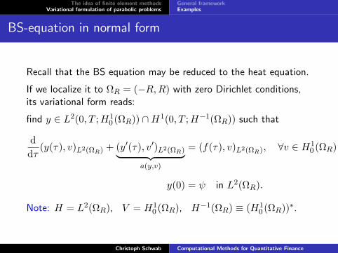
The idea of finite element methodsVariational formulation of parabolic problems
General frameworkExamples
BS-equation in normal form
Recall that the BS equation may be reduced to the heat equation.
If we localize it to ΩR = (−R,R) with zero Dirichlet conditions,its variational form reads:
find y ∈ L2(0, T ;H10 (ΩR)) ∩H1(0, T ;H−1(ΩR)) such that
ddτ
(y(τ), v)L2(ΩR) + (y′(τ), v′)L2(ΩR)︸ ︷︷ ︸a(y,v)
= (f(τ), v)L2(ΩR), ∀v ∈ H10 (ΩR) ,
y(0) = ψ in L2(ΩR).
Note: H = L2(ΩR), V = H10 (ΩR), H−1(ΩR) ≡ (H1
0 (ΩR))∗.
Christoph Schwab Computational Methods for Quantitative Finance
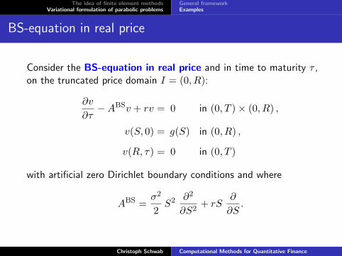
The idea of finite element methodsVariational formulation of parabolic problems
General frameworkExamples
BS-equation in real price
Consider the BS-equation in real price and in time to maturity τ ,on the truncated price domain I = (0, R):
∂v
∂τ−ABSv + rv = 0 in (0, T )× (0, R) ,
v(S, 0) = g(S) in (0, R) ,
v(R, τ) = 0 in (0, T )
with artificial zero Dirichlet boundary conditions and where
ABS =σ2
2S2 ∂2
∂S2+ rS
∂
∂S.
Christoph Schwab Computational Methods for Quantitative Finance
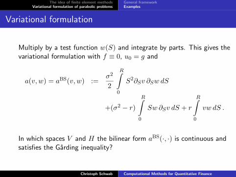
The idea of finite element methodsVariational formulation of parabolic problems
General frameworkExamples
Variational formulation
Multiply by a test function w(S) and integrate by parts. This gives thevariational formulation with f ≡ 0, u0 = g and
a(v, w) = aBS(v, w) :=σ2
2
R∫0
S2∂Sv ∂Sw dS
+(σ2 − r)R∫
0
Sw ∂Sv dS + r
R∫0
vw dS .
In which spaces V and H the bilinear form aBS(·, ·) is continuous andsatisfies the Garding inequality?
Christoph Schwab Computational Methods for Quantitative Finance
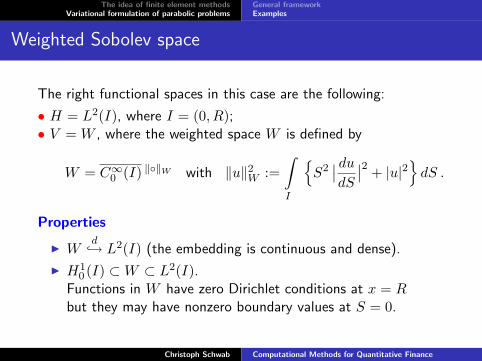
The idea of finite element methodsVariational formulation of parabolic problems
General frameworkExamples
Weighted Sobolev space
The right functional spaces in this case are the following:
• H = L2(I), where I = (0, R);• V = W , where the weighted space W is defined by
W = C∞0 (I) ‖‖W with ‖u‖2W :=∫I
S2∣∣ dudS
∣∣2 + |u|2dS .
Properties
I Wd→ L2(I) (the embedding is continuous and dense).
I H10 (I) ⊂W ⊂ L2(I).
Functions in W have zero Dirichlet conditions at x = Rbut they may have nonzero boundary values at S = 0.
Christoph Schwab Computational Methods for Quantitative Finance