empirical comparison of a of responses with -...

The Stanford Institute for Mathematical Studies in the Social Sciences

VENTURA HALL STANFORD UNIVERSITY

Reprint No. 76

Empirical Comparison of Models for a Continuum of Responses with

Noncontingent Bimodal Reinforcement

PATRICK SUPPES AND HENRY ROUANET MICHAEL LEVINE, AND RAYMOND W. FRANKMANN

Reprinted from Studies in Mathematical Psychology

19a

patguest

Typewritten Text

R.C. Atkinson (Ed.), Studies in Mathematical Psychology. Stanford: Stanford University Press, 1964, pp. 358-379.

Reprinted fr~2-i Studies i~ Mathematical Psychology, edited by R. C. Atkirzor,. Stanford University Press, 11954.

This paper is a direct extension of the earlier work reported by Suppes and Frankmann (1961). A general introduction to the problems of stochastic learning theory applied to a continuum of responses is given in the preceding paper in this volume by Suppes and Rouanet. The present experiment used the same circular apparatus as did Suppes and Frankrnann and Suppes and Rouanet. We abstract briefly from the fuller description given by Suppes and Rouanet. The response x and the reinforcement y vary continuously along the circumference of the circle from O to 2.2. l n the Suppes and Frankrnann study and also In the present study, the reinforcement is noncon'tingent, i.e., the probability distribution of reinforcement is independent of the subjects9 responses and the same distribution is used on every trial. The particular distribution used by Suppes and Frankmann was a triangular distribution on the interval O to 2n. The present study has used the bimodal distribution constructed from the two equal triafigular distributions on the interval, 8 to TZ# and n to 257 (see Fig. 2).

'Fhe aims of the present experiment have been twofold. The first has been to investigate the extent to which the common predictions of the linear and stimulus-sampling models for a continuum of responses will hold when the reinforcement distribution is no longer unimodal as it was in the case of the

This research has been supported by the United States Air Force Office of Scientific Research Directorate of Information Services, under Contract AF 49(638)-1037. Bart of the computing rehted to the analysis of data has been supported by grant USPHS ?d-6154 from the National Institute of Mental Health. We are indebted to Jean Donio and to Sylvia Garfinkel for assistance in the analysis OB dava, and to Eleanor Williamsen for assistance in running subjects.

(Henry Rouanet is now at the University of Paris, and R. W. Frankmann is at the University of Illinois.)

358

epgy

Reprinted fr~2-i Studies i~ Mathematical Psychology, edited by R. C. Atkirzor,. Stanford University Press, 11954.

Suppes and Frankmann stud?. Secondly, a larger number of trials was run in this study than in the Suppes and Frankmann study in order to provide an adequate amQLìnt o€ data at asymptote to test the differential sequential predictions af the linear and stimulus-sampling modeis. In the Suppes an$ Frankrnann and the Suppes and Rouanet studies, no predictions are reported that differentiate the ~ W C I kinds of models.

eoretical results Using the notation of Suppes and Rouanet in the preceding paper, we

may briefly summarize the theoretical results utilized in the analysis of bata. These natilrally fall into three categories.

First, there is the asymptotic response distribution whose density r ( x ) Ss given by &e equation

c 9 .(4 = Y)f(Y) 4J 2 o

where k j x ; y) is the smearing density and f (y) the noncontingent reinforcr- ment density.

and P(XB j Ya-13 These statistics are derived in the preceding article, Their equations at a s p p t ~ t e are as follows:

Sec~ad, there are the rejnforcement-dependent statistics P ( X , 1

i

where

F ( Y ) = j- V f ( Y V Y r

H ( X > Y ) = j” J- k{%?; y) j (y ) dxdy, X Y

The important thing to note about these reinforcement-dependent statistics is that like the asymptotic resporase distribution, they are the same in the linear and stimulus-sampling models.

Far the present experiment we also include the related conditional density

E ( x , Y ) = k j . x ; y ) f ( y ) dy . I ,. Third, there are the asymptotic sequential predictions l'(,Y,, 1 Y7z-l s Xn-&

Predictions of these sequential probabilities differentiate the linear and stimulus-sampling models. In the case of the linear model the result is the foliowing :

Fur the !br-element stimulus-sampling model that assiarr,es that exactly o m stimulus is sampled on every trial (i.e., the Estes pattern model), the ex- @-ession is the following:

shere c is the conditioning parameter. [In the case of statistics (21, (3), and (+j, ih terms of the pattern model c / N = Q, i.e., the sanle expression holds in the pdteern model if e is replgced by C / N : I Àn important observation that can be hade about Eq. (6) for the IW-&int%t mmdel is that it may be written itp the following form:

P ( X , I Y,:, , x ~ - ~ ) = --[Pred. o f ofiC-tteMent modell + (1 - $)R(x.,J

h other words, the sequential prediction at asymptote is a linear combination of the predictions of the one-e!ement model and the asymptotk response distribution. The rationale of this resuit is obvious. When the same dement is sampled on trials 12 and n - 1 then effectively the one-element model may be used to make predictions. The ~ ~ o ~ ~ ~ ~ ~ i t y of such an event, that is, of sampling the same element on both t d s s i s ! /N . On the other hand, if the element sampled on trial n is not the s d ~ e as the element sampled on trial M - k , then the reinforcement otl. tridl tt - i as well as the actual response made has no direct effect on the rbpohse ~ ~ s ~ r i b u t i o n on trial n, for that wil! be determined by the element sarrigled that trial. In order that this intuitive interpretation not be taken literally, however, it shouki be

(6') 1 N

B I R I O D A L C O N T l N G i U h i O F R E S P O N S E S 361

pointed QU^ that the precise rcsult givcn here does not hoid except at asymptote. 'The rc3sons for this may be seen by examining the detailed derivation given in rhe Appendix.

2. ~ x ~ e ~ ~ ~ ~ ~ ~ ~ ~ method Subjects. The subjects were 4 male and 26 female Stanford under-

graduates. Each subject w\\';?s paid $2.50 for the two-hour experimental session. A~~~~~~~~~ The germa1 apparatus is the one described in Suppes and

Frankmann (196f), but of the two circles, only the larger ( 5 feet in diameter) was used in the present study.

ure. 'The instructions to subjects, describing the experiment as a target prediction problem, were identical to those used in the Suppes and Frankrnann study, 4 t h one exception. In the earlier study when the bar of red light was moved around the circumference of the circle at the beginning OE the instructions, it was stopped at the top of the circle. h the present study it was stopped at the randomly selected physical position for the scale zero of a giver, subject.

As soon as questions had been answered by paraphrasing the instructions, 606) triais were run, with one interruption of abmt 3 minutes after the 300th trial, The average rate was 6 triais per minute.

. A411 subjects were run under the same experimental conditions. trial reinforcement sequences were computed using the bimodal

density shown in Fig. 2. By random choice, 30 equally spaced divisions of the circle, starting from an arbitrary physical zero, were assigned without repetition as scale zero points for the separate reinforcemcnt sequences.

The presentation of results has been organized into the following cate- g~ries: conditional variance learning curve; estimation of parameter of smearing distribution; asymptotic response distribution; estimation of learning parameter; goodness of fit of reinforcement-dependent statistics; and ~ o ~ e ~ - ~ ~ ~ e r ~ ~ ~ ~ ~ ~ ~ n g sequential statistics.

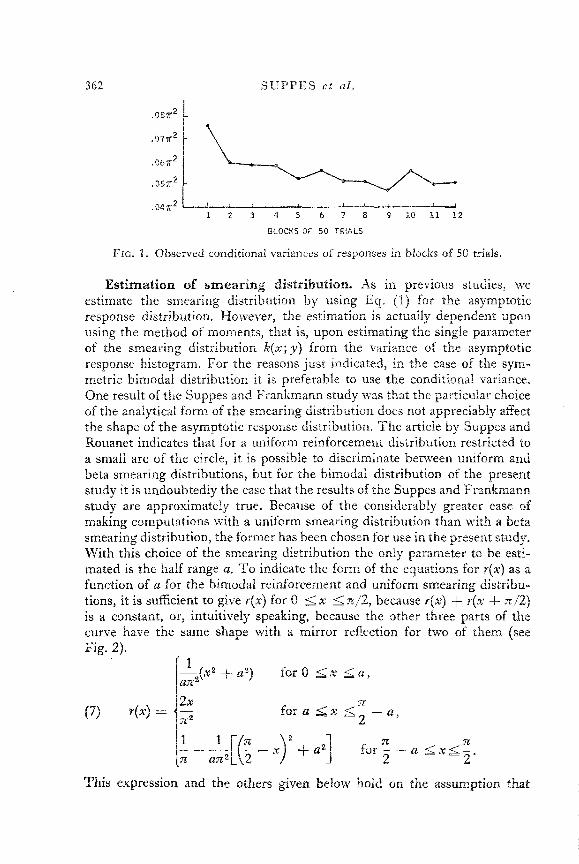
~~~~~~~Q~~~ ~~~~~~~~ ea^^^^^ curve. In previous studies w e have found that the varianw learning curve provides a good index of the rzte of learning. In the case 5f a symmetric bimodal reinforcement diSt?ibUliQn, such 'as was used in the p resa t study, the variance i s not a sensitive measure of learning. There is, however, B natural substitute, namely, the conditional variance, Le., the variance of the c ~ n d i t i o d distribution restricted to ha1.f of the cide. Figure 2 shows the observed variance of the empirical conditional distribution on the interval 0 to 7c combined with that on z to 2z in blocks of fifty trials. It is evident that the variance ia very close to an asymptote at the end OE the first 100 trials and is essentially constant from trials 200 to 600. The asymptotic results that foollow are based on the last 400 trials of the experiment.

362

Estimation of ~~~~~~~~ ~ ì § ~ ~ ~ ~ ~ t ~ ~ ~ . As in previous studies, we estimate the smearing distribution by using Eq. (1) for the asymptotic response distribution. MoweT;er, the estimation is actually using the method of moments, that is, upon estimating the single parameter of the snearing distribution k ( x ; y ) from the variance of the asymptotic response histogram. For the reasons just indicated, in the case of the symmetric bimodal distribution it Ss preferable to use the conditional variance, One result of tke Suppes and Frankmann study was that the particular choice of the analytical form of the smearing distribution, does not appreciably afTect the shape of the asymptotic response distribution. The article by Suppes and Rouanet indicates that for a uniform reinforcement distribution restricted to a small arc of the circle, it is possible to discriminate between uniform and beta smearing distributions, but for the bimodal distribution of the present S F U ~ Y it is undoubtedly the case that the results of the Suppes and Frankmann study are approximately true. Because of the considerably greater ease af making computations with a uniform smearing distribution than with a beta smearing distribution, the former has been chosen for use in the present st.udy. With this choice of the smearing distribution the only pararneter to be estimated is the half range a. T o indicate the form of the equations for ~ ( x ) as a function of a for the bimodal reinforcement and uniform smearing distributions, it is sufficient to give ~ ( x ) for O I x i n/2, because Y(.) + r(x i n/2) ìs a constant, or, intuitively speaking, because the other three parts of the curve have the same shape with a mirror reflection for two of them (see Fig. 2).

This expression and the others given below hold on the assumption that

13ISIODA.L C O N T I N U L T L ~ O F R E S P O N S E S 363

Q < zi4? n.I:ich t u n s out not to he 3 red restriction, for the estimate of a falls definitely heiow this upper bound. It may he noted from Eqs. (7) that. .(x> coincides with the reiaforcement densityj(y) for x between u and x, /2 - a.

From (7) it is straightforward to derive that the asymptotic conditional variance (C.V.) on the interval 0 to z is given by the i o l l ~ ~ i n g expression as a function of a ,

From the natural symmetry of the circle, it is seasonahle to combine the conditional variance computations for the two intervals (O, ;z> arad (z> 2x1 in order to use al? the data. More precisely, for each response in the last 400 trials we computed its squared deviation about the mean of that one cjf the two intervals in which it fell, and then divided the sum of these deviations by “62,000, the number of responses; to obtain the empirical estimate of the conditional variance. AS a partial behavioral check on this rather obvious assumption of symmetry, we tabulated, as shown in Table 1, the number of responses falling in each interval for each subject. The en the null hypothesis that there are exactly 20@ responses in each interval is also shown foor each subject. The responses of subject 21 show a highiy significant deviation from the nuil hypothesis of symmetry. When his = 116.64 is subtracted from the total, the resulting is 37.44, which with 29 degrees of freedom is

212 188 1 ..e4 180 220 4.00 206 294 .36 195 205 .25 194 206 .36 212 188 1.44 220 k80 4.00 198 202 .o4 189 211 1.21 208 192 .64 189 211 1.21 215 185 2.25 200 200 ~ 0 0 184 214 1.96 P93 207 ~ 49

182 218 3 2 4 206 P94 .36 201 199 .QI 200 200 .o0 205 194 .36 92 308 116.64

887 213 1.69 207 193 .49 223 177 5.29 205 195 .25 192 208 .64 I96 204 .l@ 195 205 .25 219 181 3.61 212 188 3.44

364 SUPPES E i af.

not significant at the .IO jevel. Bata frort? subject 21 are retained in ali the empirical computations given in the remainder of the papper, although some improvement of fit would have resulted from omitting his protocol.

Using the computation described, the empirical conditional variance is n051684z2e On the basis of Eq. (S), this leads to the estimate a* = #1930n, and this value is used in the remaining theoretical predictions reported.

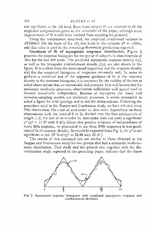
presents the response histogram for the group of subjects in class Intervals of .O53 for= the last 400 trials. The predicted asymptotic response densi<? rhx)? as well as the triangular reinforcement density f ( y ) , are also shown dn the figure. It is evident from the most casual inspection that the response density rex> fits the empirical histogram of responses extremely weli. In order to perform a statisrical test of the apparent goodness of fit of the response density to the response histogram, it is necessary for the validity of the test to select observations that are statistically independent, It is w d l known that for stationary stochastic processes, observations sufficiently weBB spaced tend to become statistically independent. Because at asymptote the h e a r and stimulus-sampling models are stationary processes, it seems reasonable to select a figure for trial spacings and to test for independence, Following the procedure used in the Suppes and Frankmann study, we have selected every fifth observation. o n a test of zero-order vs. first-order dependeme on these observations with :he interval 8 to 2n divided into the four subintervals QE length n/'2> the test of zero-order vs. first-order does not yieid a significant x 2 (x2 = 11.24 with 9 df). Given this positive evidence of independence of every fifth response, we proceeded to use these 2400 responses to test goodness of fit of response density. As would be expected from Fig. 2, the x 2 is not significant at the .O5 Bevel ( x 2 = 52.44 with 38 d€).

The results of this statistical test are similar to those obtained in the Suppes and Frankmann study for two groups that had a unimodal reinforcement distribution. That study and the present one, together with the dis- crimination study reported in the preceding paper, indicate tbat the h e a r

GQQdne§§ 0%' fit O f aSyPnm totie: respo"§" ~ ~ S ~ ~ ~ ~ ~ t ~ ~ ~ . Figure 2

o - 76 311 2 2

FIG. 2. Asymptotic response histogram with predicted asymptotic response a d

256

reinforcement densities.

BI; \ IODAL C O N T I N C ' U L I O F R E S P Q N S Z S 365

and sti~ilulus-sampli~l~ Inodcls for a continuui11 of rcsponscs are nble to predict x , \ . i t h goad quantitative accuracy the asymptotic response distribution on the basis cf estinlaring a single parameter, nanrely, the parameter of the smearing distribution.

st^^^^^^^ ea^^^^^ parameter. T o analyze the goodness of fit of the reinforcement-depcndeIlt statistics, it is first necessary to estimate a second parameter, In the linear nlodel this parameter is usuaiiy designated as the learning parameter O. In the stimulus-sampling pattern models it is the Iearn- ing parameter c i S , where c is the probability of conditioning the stimulus pattern sampled QII each trial, and N is the number of stimulus patterns available for sampling. I t shou'rd be noted that at the level of the reinforcement-dependent statistics it is not possible to make separate estimates of t and ?d but only to esFinlate the ratio c/lv.

2200

2000

1800

l b 0 0

14 O0

1200

x 2 a000

800

b00

4 O 0

200

O I I l I l l I .O8 . I b .24 .32 ,40 .48 .56 ,

c O -E

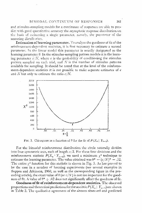
FIG. 3. Chi-square as a function of B for the fit of P ( X n 1

4

For the bimodal reinforcement distribution the circle naturally divides into four symmetric arcs, each of Iength n/2. For these four divisions and the reinforcement statistic P ( X , 1 Y,,-,), we used a minimum x 2 technique to estimate the learning parameter. The value obtained was O* == ( c / N ) * = .32. The entire x 2 function for this statistic is shown in Fig. 3. As has proved to be the case in a number of learning experiments (see several examples in Suppes and Atkinson, 1950, as well as the corresponding figure in the preceding article), the exact value of O (or & / N ) is not too important for the goodness of fit. A value of O* & .O2 does not significantly affect the goodness of fit.

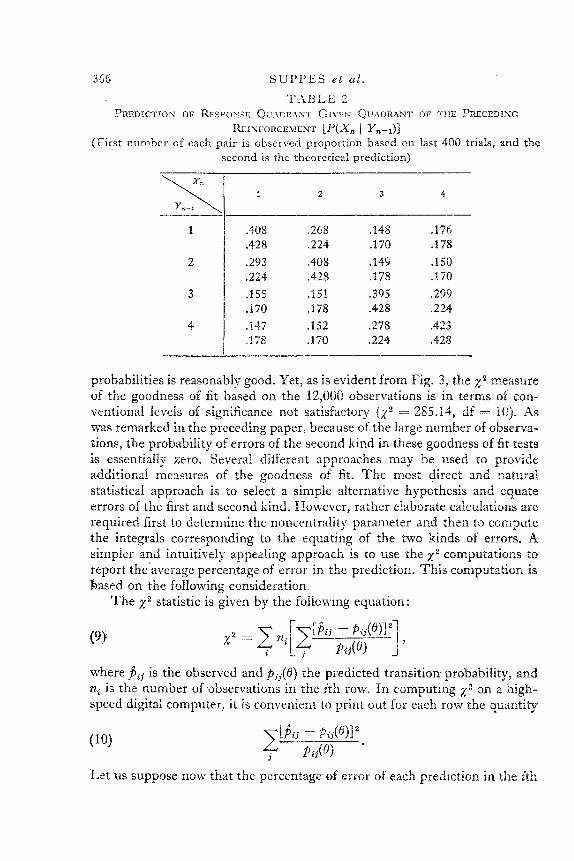
Goodness of fit of reinbbrcemeabt-depelndent statistics. The observed proportions and theoretical predictionsfor the statisticP($jL 1 are shown in Table 2. The qualitative agreement of the sixteen observed and predicted

2 3 4

.268

.224

.408 ,428 .d51 .l78 . l52 . l70

.l48

.l 70 ,149 .l78 .395 .428 .278 ,224

probabilities is reasonably good. Yet, as is evident from Fig. 3 , the measure of the goodness of fit based on the 12,000 observations is in terms of conventional h e l s of significance not satisfactory (x2 = 285.14, df =- 18). As was rernerked in the preceding paper, because of the large number Q€ ob- aerva- tions, the probability of errors of the second kind ir, these goodness of fit tests

essentially zero, Several different approaches may be used to provide additional measures of the goodness of fit. The most girect and natura! statistical approach is to select a simple alternative hypothesis and equate errors af the first and second k i d . However, rather elaborate calcula+' L I O ~ S are required first to determine the noncentrality parameter and then +LO c ~ m p u t e the integrals corresponding to the equating of the two kinds of errors. A simpler and intuitively appealing approach is to use the xa cornputat: '011s t0 report the.average percentage of error in the prediction. This computation is b s e d on the following consideration.

The x 2 statistic is given by the following equation:

where jij is the observed and p i j (@) the predicted transition. probability, and ni is the number of observations in the i h row. In computing x 2 on a high- speed digital computer? it is convenient to print out for each row the quantity

Eet us suppose now that the percentage af error of each prediction in the ith

368 S U P P E S e t n l .

the reinforcement event is the first quadrant on the Ieft in the top figure, and that is the scco~ld quadrant in the bottom figure. The remoteness of the point-sdjacent quadrant P in the top figure is deceptive because the figure does not show the periodicity of the circle. $Te call this the SLAP reduction of ;he 4 X 4 table.

In order to check that this reduction of the data has been approximately guaranteed by the experimental design, a x 2 test of goodness

x of fit was run with the four e m p i r i d SLAP numbers as the parameters. It is to be empha- sized that this test in no way depends ca the parameters of the models. We simply considered the 4 X 4 matrix of transition probabilities P(XtL 1 and used as “theoretical” p r o b a ~ ~ ~ i ~ ~ e s t h e ~ o u r estimated SLAP numbers

FIG. 4, Diagram illustrating the With 8 net degrees of freedom, the resulting SLAP relations. x 2 = 20.47 is just significant at the conventional

.O1 Bevel, but €or the large number oh observations the fit is excellent. In terms ofthe concept of ‘*average” error introduce above, e is less than 4 per cent.

Applying the SLAP reduction to the observed data, we conpare in Table 3 the observed and predicted probabiiities for the four SLAP quadrants. The x? measuring the goodness of fit is comparable ( x 2 = 261.02) to that obtained. for the unreduced data of Table 2.

In certain respects the kind of presentation provided by Table 2 and Tabie 3 belies the continu~us character of the reinforcement and response distributions.. A more detailed and instructive picture of the behavior of subjects with respect to the r e i l . , f~ rcennen t -ce~e~de~~ statistics is given by the conditional densities corresponding to the discrete densities shown in Tables 2 and 3. We have used the symmetries implied by the SLAP test to construct a single conditional density j ( ~ , ~ j The observed histogr and predicted density are S ~ Q W ~ in Fig. 5. The f igxe is drawn f5r the SL data with Y,L- I always placed as the interval (z, $z)- The qualitative agreement between the observed histogram and the predicted density is quite good. The

I Î S L x P

O S S . E .409 ,284 .as1 .l56 Pred. I .428 .224 .l70 .l78

l

o R ? X

FIG. 5. Observed response histogram conditioned upon preceding I’ekkfQrCWflent with corresponding predicted density j (xTL 1 l’n-,).

two most important characteristics of the predicted response density that are nel! confirmed in the data shou’ld be noted. One is the asymmetry of the predicted distribution. The other, which is more subtle and much less likely to be predicted without a definite quanritatlve theory, is the secondary peak or wave in the density for the half of the circHe in which a reinforcement did not occur. On non-theoretical intuitive grounds one natura? prediction would be that the response densiry monotonically decreases away from the quadrant in which a reinforcement occurred. The prediction of the wave as opposed to a monotonicaiiy decreasing function is wel! supported by the empirical data.

YTL-2) . The qualitative agreement between the 64 observed and predicted probabilities for the four quadrants is reasonably good, but d e h i t e quantitative discrepancies do occur, as 4s reflected in the that has a value of 1343.8 with 46 df. T o exahine these discrepancies more closely and yet reduce considerably the number of quantities to be considered, we have been able to apply the SLAP method of reduction to reduce the 16 X 4 table of second- order statistics to a 4 x 4 table. As in the case of Table 3, we first p e ~ ~ 5 ~ ~ ~ ~ a x 2 test of homogeneity to justify the SLAP reduction of the datz. The results were not significant ( z z = 35.80, df = 32, and P > .30).

The observed and predicted probabilities are shewn in Table 1. A word. of explanation is perhaps required about the use of the SLAP coordinates in the case of the second-order statistics. ‘-she row designations refer to the relations between the two reinforcements, and the column designations for the response X,, refer to the SLAP relation between the response quadrant pi, and the reinforcement

Inspection of row P of Table 1 indicates what is perhaps the most serious discrepancy in the prediction of the second-orde: reinforcement statistics. ‘l’he observed proportions for C Q ~ U ~ I I L fit almost exactly the predicted probability for column P, and the observed proportions for column almost exactly the predicted probability for colunnxa L. Analysis of Eq. (3)

I V e turn now to the second-order reinforcement statistics P(Xa j

FIG. 6. Observed response histograms conditioned upon two preceding reinfxcernents with ccrrespordirlg predicted densities.

A j ,394 ,287 .l68 .l51 .374 . i75 .z91 .IS0

.314 .l48 . l50 “380 .l69 . l 5 2 .z99

indicates that no simple change in the learning parameter cmld seriously improve these predictions. The difficulty is that: the theory predicts much stronger effects for the second preceding reinforcement than in fact it seems to be having, We have the somewhat unexpected circumstance that if we compute the fit of the theoretical P(XZ1 j Y,(-:) m the second-ordes statistics given in Table 4, the fit is better than that of the predictions shown in the table. Adjustment of the parameter of the smearing distribhition would improve the Pit of the theoretical second-arder reinforcement statis~ic to the observed data. It is evident from Eq. ( 3 ) that the value of the function H ( X , ~ must increase considerably to account for the discrepancies in row P, beat to increase this function in the case of column L a very substantial increase in the range of the smearing distribution is required. Such an adjustment would seriously disturb the excellent fit of the asymptotic response distribution, as shown in Fig. 2.

As would be expected from Table %, when we turn to the conditional densities j(xTL j k’n-ls the worst fits are for the A and P cases of the SLAP reduction. It is in these two cases that Y7t-l and are most different, and from an empirical standpoint the theory errs in attaching too much importance to the reinforcing egects of YR-2 p as is apparent fmm Fig. 6. The figures are drawn for the SLAP data with Y,-x always placed as the interval (x, +c). The notation j ( x?& j SIL-- i , p z - 2 ) in Fig. h , for instance, means that this is the conditional density for and being the same interval; similar SLAP definitions apply forj(x,, j Ln-l7 n.-2j,j(xn 1 An-l n--l$,

and j ( x n j Pn-l! T h e large secondary wave in the predicted curves €or the A and P cases (Figs. 6c and 6 d ) result from the weight, given Yn--2 and are simply not substantiated by the data, although there Is a small secondary

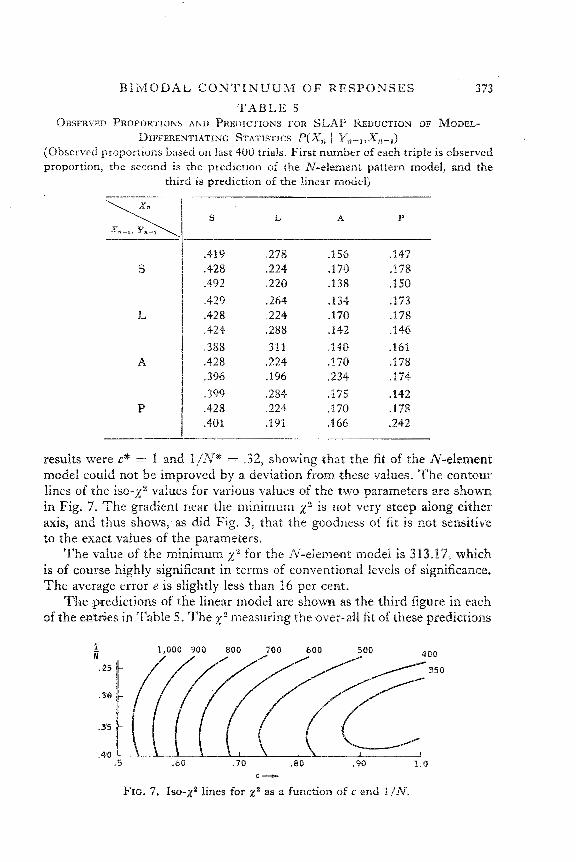
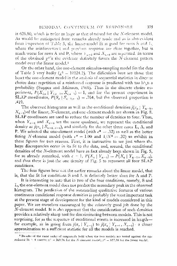
results were P = I and 1/N" = .32, showing .that the fit of the N-element model could not be improved by a deviation from these values. The contoua: lines of the iso-x2 values for various values of the two parameters are shown in Fig. 7. The gradient near the minimum is not very steep along either axis, and thus shows; as did Fig. 3, that the goodness of fit is not sensitive to the exact values of the parameters.

The value of the minimum for the N-eleme-nt model is 3 13.17, which is of course highly significant in terms of conventional levels of significance. The average error e is slightly less than 16 per cent.

The predictions of the linear model are shown as .the third figure in each sf the enx,ries in Table 5. The x 2 measuring the over-all fit of these predictions

F L 1,000 900 800 700 600 500 O0 .25 350

.38

.s5

.40 .5 . t o .70 .85 . so 1.0

C-

FIG. 7. Iso-x2 lines for x2 as a function of c and

one-element mcdei 7/\

N-element mcdel

n 271

N-element d e l

ole-elemeo! mudel

O f l

N-element (,.cdel -

O 2x

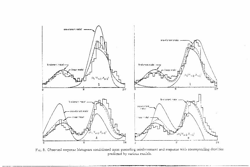
FIG. 8, Observed response histogram conditioned upon preceding reinforcement a r d response with corrcspnnding d e n d i e s predicted by various rr?odeis,

3 76 S U P P E 5 e t a l .

4. S1Jmnnnai-y Statistical learnkg theory %-as been g-neral.ized to produce models for the

study of learning phenonlena i n which both responses and reinf~orcemrnts are measured on a c o n t i n ~ o ~ ~ scale. ‘l’kis paper reports another empirical test o€ these models.

Subjects were instructed to predict, in a sequence cd600 triais, the position of a point target on the circumference of a circle. In fact, the correct positions of the target-the *einforceraaents-wpse independent samples from a fixed distribution having a symmetric, birnodzl density.

Ail of the modeis considered predict the same asy~nptotic m~conditional respome distribution and conditional resp~nse distribution wtienever the conditioning e17ent specifies only reinforcements. The correspondence between the cbserved and predicted asymptotic response distribution is strikingly close. Predictions of the conditional densities range from f2ir to excellent. One unanticipated finding (namely, a secondary peak in the conditional response densities) Ss weli described by the modeis.

‘khe models diaex. in their predictions of conditianal response distrihutions if the conditioning farent specifies a preceding response. 03 the basis of these statistics, one easily rejects the one element n~obel. Bath the iV-element and ‘tinear n ~ d e l s predict the outstanding qualitative characteristics of these conditional distributions, hut the ?<-eIemerrt model, being better able ta emphasize the effects sf the most recerrt past, more precisely describes the data.

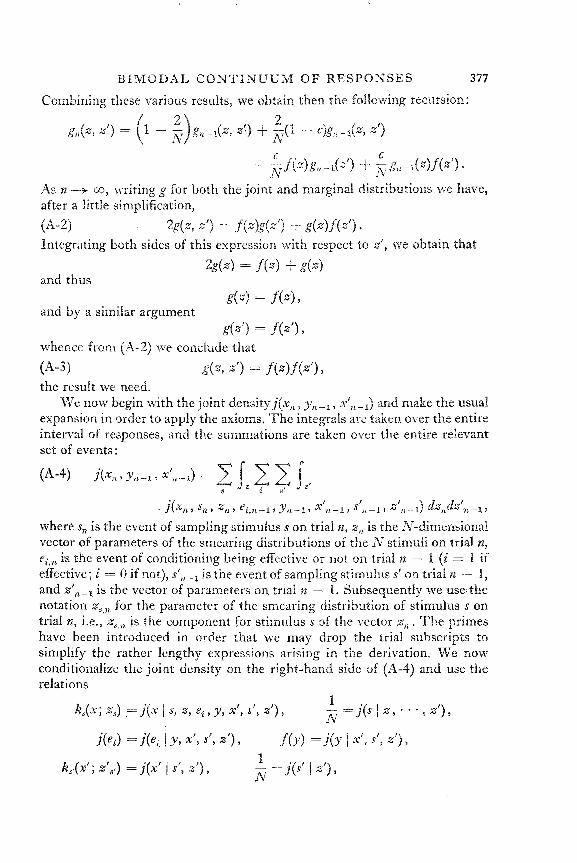
As n ,---f c o , writing g for both :he joint and marginal distributions we Rave, after a little simplification, (11-2) 2g(q d) = f(z>g(z’) * g(.)f(x’). hegrat ing both sides of this expression with respect to Z‘, we obtain that

and thus

and by a similar argument

whence fronl (A-2) w e conclude that

= j-(z) + g(.>

g(::) = $(z> Y

g f 4 = f ( X ’ > >

(A-3) g(z, 2‘) = f(z)f(z’) the result we need.

W e now begin with the joint densityj(x,, , xilL--I j and make the usual expansion in order to apply the axioms. T h e integrals are taken over the entire interval of responses, and the salmnlations are raken over the entire relevant set of events:

. jix.,L 5 S,L P Z,, > e>¿, lL-l 7 Y,1-1 9 x*/L-z $’,l -1 9 x!,, -3 &JZ’:l,,-1 t

where s, is the event sf sampling stinlulus s on trial n, z,, is the N-dimensional vector o i parameters of the smearing distributions of the N stimuli on trial ns ei,% is the event of conditiorJng being effective or not on trial z - 1 (i = 1 if effective; i = O if not), S‘,! .I is the event of sampling stimulus s‘ on trial n -- I , and z ’ / % - ~ is the vector of parameters on trîai n - I. Subsequently we use.the notation x,,, for the parameter of the smearing distribution of stimulus s on trial v , i.e., i s the component for sti~nulus s of the vector x,. The primes have been introduced i j l order that we may drop the trial subscripts to simplify ehe rather Icngthy expressions arising i~ the derivation. We now conditionalize the joiilt density on the right-hand side of (A-4) and use the relations

1 N #+,(x; z,) ,= j(x 1 s, x, P i , y, X’, S’, X’), - = j ($ I z , * . * z ! ) ,

./(ei) = j(.;, ! Y , x’, S’, 2’) s f(y> = j ( y 1 x!, S’; X’), 1 ni

K,.(x.’; Z’,.) = j(x’ j d , :a ’ ) , .- T= j($’ 1 Z’> ~

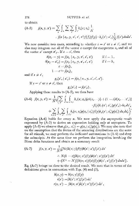
378 SUFYES e t a l ,

to obtain

We now consider two cases, according to whether S = s’ or s # S’, and we also may integrate out all of the vector x except the component ,zs and all of the yector z’ except Z’,, . If s = S‘, then

6(x8, - y ) = j ei t y, X’, S’, X’) i f i - 1, 6(z,* - d s . ) 1 “ i , y, X’, S’, Z’) i f i = o ,

i =A4 I

1 - c..; j ( e , ) s and if s # sØp

g&’, j ZP8,) = j ( x s I 6 2 6 , y, XI, S’, Z’) i

91L(xrs~) = j W e , >

If s = s’ or .Y # S‘, then

Applying these results to (A-S>, we then Rave

Equation (A-6) holds for every n. We now apply the asymptotic result expressed by (A-?) to derive an expression holding at asymptote. To apply (A-3) we observe that g ( x s , x,:.) = g(xs j x:.)g(z;.>. We may also note that on the assumption that the forms of the smearing distributions are th, - same for all stimuli, we may perform the indicated summations in (A-6) and drop the subscripts. A.t the same time we perform the integrztion involving the Dirac delta functions and obtain as a summary result

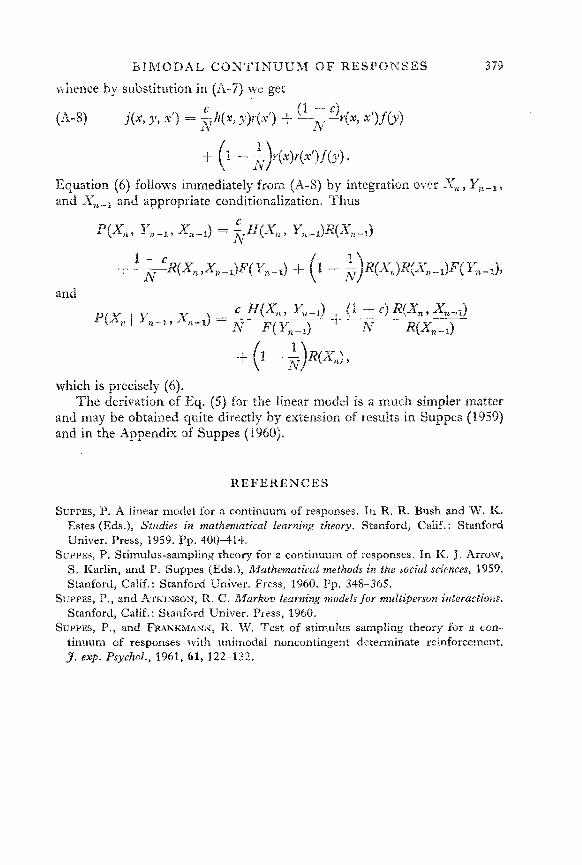
which is precisely (6). The derivation of Eq. (5) for the lisiear model is a much simpler matter

and may be obtained quite directly by extension of results in Suppes (8959) and in the Appendix sf Suppes (1960).

R E F E R E N C E S

SUPPES, P. A linear model for a continuum of responses. h R. R. Bush and W. K. Estes (Eds.), S t ~ ~ d i e s in mathematical learning theory. Stanford, Calif. : Stanford Univer. Press, 1959. Pp. 400414,

SUPPES, P. Scirnulus-sampling theory for a continaurn of responses. In K. J. Arrow, S. Karlin, and P. Suppe:s (Eds.), Mathematical methods 213 the social sciences, 1959. Stanford, Calif.: Stanford LTniver. Press, 1950. Pp. 348-365.

SUPPES, P., and ATKINSON, R. C. Markov learning models for mulhiperson interactions. Stanford, Calif. : Stanford Univer. Press, 1960.

tinuurn of responses with unimodal noncontingent deteminate reinforcement. SUITES, P., and FRANKMANN, n. w . Test O f Stil l luiUS Sanlphg theory fQr B COPZ-

J. ex@. Psychol., 1962, 6 4 , 122-132.

empirical comparison of a of responses with -...

Documents