l Estes’ Statistical Learning Theory: Past, Present, and Future

Patrick Suppes Stanford University

THE PAST

The direct lineage of statistical leaning theory began in 1950 with the publica- tion in Psychological Review of Estes’ article “Toward a statistical theory of learning.” Before saying more about that I recall, however, that there were a number of earlier attempts to develop a quantitative theory of learning which can easily be cited, but I hasten to say that I am not attempting anything like a serious history of the period prior to 1950. I have used the following highly selective but useful procedure of listing the earlier book-length works referred to in the spate of important papers published between 1950 and 1953, which I discuss in a moment. The earlier references referred to (not counting a large number of articles) are Skinner’s Behavior of Organisms, published in 1938, Hilgard and Marquis’ Conditioning and Learning, published in 1940, Hull’s Principles of Behavior, published in 1943, and Wiener’s Cybernetics, published in 1948. These and other earlier works not mentioned played an important role in develop- ing the theoretical concepts of learning used in statistical learning theory and related theories developed by others shortly thereafter. The basic concepts of particular importance are those of association and reinforcement expanded into the concepts of stimulus, response, and reinforcement, and the processes of stimulus sampling and stimulus conditioning. Other important psychologists who contributed to this development and who were not mentioned on the basis of the principle of selection I used are Guthrie, Thorndike, Thurstone, Tolman, and Watson.

The work of all these psychologists would seem to be almost a necessary preliminary for detailed quantitative and mathematical developments. (Wiener’s

1

of 1953 a number of important theoretic articles had appeared that set the tone for another decade. I mention especially and in chronological orde the two Psycho6ogicu6 Review articles in 195 1 of Bush and Mosteller, which presented in clear and workable mathematical fashion models of simple learning and models of stimulus generalization and discrimination; the 1952 article by George Miller on finite Markov processes; and the 1952 article by Miller and McGill on verbal learning. I end with the 1953 Psycho6ogicul Review article by Estes and Burke on the theory of stimulus variability. These are not the only articles on learning that appeared dwing this period, nor even the only theoretical ones. But they are by the psychologists who created a new theoretical approach in psychology. To an unusual degree, Estes’ 1950 article marks in a very definite way the beginning of this new era*

My own involvement with Bill Estes and learning theory began after 1953. We first began to work together in 1955 when we were both fellows at the Center

1. ESTES' STATISTICAL LEARNING THEORY 3

for the Advanced Study in the Behavioral Sciences at Stanford. It is probably fair to say that I learned more about learning theory in the fall of 1955 in my almost daily interactions with Bill at the Center than at any other time in my life. He brought me quickly from a state of ignorance to being able to talk and think about the subject with some serious understanding. I had previously tried to read the works of Hull mentioned earlier, but had found it fairly hopeless in terms of extension and further development, for the reasons already indicated. Once Bill began explaining to me the details of statistical learning theory I took to it like a duck to water, because I soon became convinced that here was an approach that was both experimentally and mathematically viable.

Over the years I have become involved in other aspects of mathematical psychology, especially the theory of measurement, the theory of decision mak- ing, and the learning of school subjects such as elementary mathematics. In the process I have had the opportunity to work with colleagues who have also taught me a lot, particularly Duncan Luce, Dave Krantz, Amos Tversky, Dick Atkin- son, and Henri Rouanet. But although many years have passed since Bill and I worked together on a regular basis, I still remember vividly my own intellectual excitement as we began our collaboration in that year at the Center.

More generally in the 10 years following that initial burst of activity from 1950 to 1953, Bill had many good students and much good work was published both by him, his colleagues, and his students. In fact, in my own judgment the decade and a half from 1950 to 1965 will be remembered as one of those periods when a certain new approach to scientific theory construction in psychology had a very rapid and intense development, perhaps the most important in this century.

THE PRESENT

I think it is fair to say that in the 1970s and 1980s much of Bill's own interests shifted from learning theory to problems of memory and related areas of cogni- tion. During this period the new wave of enthusiasm was for cognition rather than for learning. Fortunately, in the last few years we have had a return to a central concern with learning in the recent flourishing of connectionism and the widespread interest in neural networks. It is apparent enough that many of the new theoretical ideas have a lineage that goes back to the developments in learning theory between 1950 and 1965.

I am not going to try to give a survey of these new ideas (see Suppes, 1989), but rather give three applications that arise out of statistical learning theory and related work on stochastic models of learning in the 1950s. These applications are also not meant to be a survey, but reflect my own current work. My purpose in discussing them is to show how the basic ideas of statistical learning theory remain important and have the possibility of application in quite diverse areas of theoretical and practical concern.

given day includes exercises from a selection of the strands appropriate to the student’s grade level. In general the exercises are selected across the strands on a random basis according to a curriculum distribution, which is itself adjusted to be a convex mixture with a purely subjective distribution depending upon the indi- vidual student’s strengths or weaknesses. The curriculum probability distribution is itself something not to be found in the general theory of‘ curriculum in textbooks, but is essential to the operational aspects of the kind of course I am describing- I do not here, however, go into the details of either the curriculum distribution or the individual student distribution, nor do I discuss the equally

- important problems of contingent tutoring when the student makes a mistake, or how a student is initially placed in the course.

The detailed use of learning theory occurs in monitoring and evaluating when

1. ESTES' STATISTICAL LEARNING THEORY 5

a student passes a mastery criterion for leaving a given equivalence class of exercises to move on to a more difficult concept or skill. Here we have been able to apply detailed ideas that go back to the framework of statistical learning theory introduced in Bill Estes' 1950 paper, but with an application he probably never originally had in mind: to the daily activity of students in schools in many parts of the country. Classical and simple ideas about mastery say that all that is needed is a test. On the basis of the relative frequency of correct answers in a given sample a decision is made as to whether the student shows mastery. But the first thing that one finds in the detailed analysis of data is that when a student is exposed to a class of exercises, even with previous instruction on the concepts involved, the student will show improvement in performance. The problem is to decide when the student has satisfied a reasonable criterion of mastery.

The emphasis here is on the data analysis of the actual learning, not on the setting of a normative, criterion of mastery. For this purpose some standard notation is introduced. Although in almost all of the exercises concerned, the variety of wrong student responses is large, I move at once to characterize responses abstractly as either correct or incorrect. With this restriction in mind I use the following familiar notation:

= event of incorrect response on trial n,

Al,n = event of correct response on trial n,

X, = possible sequence of correct and incorrect responses from Trial 1 to n inclusive,

q, = P(AoJ, the mean probability of an error on Trial n,

4 = 41,

Also, and _A1 are the corresponding random variables. The learning model that Zanotti and I have applied to the situation described is

one that very much fits into the family of models developed by Estes, Bush, Mosteller, and the rest of us working in the 1950s. In addition to q, there are two parameters to the model. One is a uniform learning parameter (Y that acts con- stantly on each trial, because the student is always told the correct answer; and the second is a parameter w, which assumes a special role when an error is made. This is one way to formulate the matter. A rather more interesting way perhaps is to put it in terms of the linear learning model arising from statistical learning theory analyzed very thoroughly in Estes and Suppes (1959, 1959a, 1959b). The parameter (Y corresonds to 1 - 8 in the linear model derived from statistical

- learning theory. The linear learning model derived from statistical learning theo- ry puts all of the weight as such on the reinforcement. The generalization consid- ered here is straightforward and can be found in earlier studies as well. In terms

is

Q 1 2 3 4 5 6 7 E 9 10 11 l2 13 14 15 16 17 18 19 20

Tnals

FIG. 1.1. Addition at grade-level 3.65, sample size = 612, Q = 0.545, &O = 0.847.

_.

1. ESTES' STATISTICAL LEARNING THEORY 7

YI 8 O

u) L

B m U

U

FIG. 1.2. Multiplication exercises at grade level 3.65, sample size = 487, 4 = 0.508, ¿i = 0.875.

for example, 3.65 for multiplication. But this does not mean that all the students doing these exercises were in the third grade, for with the individualization possible, studeilts can be from several different chronological grade levels. The sample sizes on which the mean curves are based are all large, ranging from 406 to 616. The students do not come from one school and certainly are not in any well-defined experimental condition. On the other hand, all of the students were working in a computer laboratory run by a proctor in an elementary school so there was supervision of a general sort of the work by the students, especially in terms of schedule and general attention to task. In these mean learning curves and the sequential data presented later, the students who responded correctly to the first four exercises have been deleted from the sample size and from the data, because in terms of the mastery criterion used, students who did the first four exercises correctly in a given class were immediately moved to the next class in that strand. No further deletions in the data were made. For each figure the estimated initial probability q of an error and the estimated learning parameter OL

are given. The data and theoretical curves shown in Figs. 1.1-1 -4 represent four from a

sample of several hundred, all of which show the same general characteristics;

s B

etween two fraction exercises there might well intewen cises, one a word problem, another a decimal problem, and so on. Also, it is probably true for all of the students that they had had some expos~e by their classroom teacher to the concepts used in solving the exercises, but, as is quite familiar from decades of data on elementary-school mathematics, students show clear improvement in correctness of response with practice. In other words, learning continues long after formal instruction is first given. The most dramatic example of an improvement is in Fig. 1.4. This is not unexpected, because understanding and manipulation of fractions are among the most difficult con- cepts for elementary-school students to master in the standard curriculum,

In Tables i . f - 1.4, data from the same four classes of exercises are analyzed in terms of the more demanding requirement on the learning model to fit the sequential data. In the present case we looked at the first four responses with, as already indicated, the data for students with four correct responses deleted. This left a joint distribution of i5 cells, and in the case of the sequential data, the

1. ESTES' STATISTICAL LEARNING THEORY 9

1 Z 3 4 5 6 7 8 9 10 11 12 13 14 15 l6 17 l8 19 ZO

Tnals

FIG. 1.4. Fraction exercises at grade level 4.40, sample size = 616, 4 = 0.849, â = 0.736.

TABLE 1.1 Observed and Theoretically Expected Distribution for the First Four Responses to Addition

Exercises at Level 3.65. Sample Size - 612, DF = 11. W = 0.188. q = 0.406, ¿i - 0.750, x2 - 14.39

CeIl Observed Expected

O000 25 20.6 O00 1 36 35.0 O01 o 19 21.1 O01 1 75 70.6 O100 13 15.6 O101 34 39.3 o1 10 31 25.5 o111 163 151.6 1 O00 12 12.7 1 O01 19 27.3 1010 19 17.3 101 1 60 80.0 1100 18 14.6 l101 49 48.3 1110 39 32.6

Sample Size - 406, DF - 11, i, - 0.188, ij = 0.281, â = 0.7

0000 O00 1 OOlQ O01 4 O100 0101 o1 10 o11 1 l O00 1 OOI 1010 101 4 l100 1101 1110

12 12 9 29 10 23 21 115 8 47 13 54 8 43 32

9.4 16.0 10.5 36.3

8.6 22.3 15.6 103.4 8.2 18.1 12.4 62.6 11.5 41.3 29.7

1. ESTES' STATISTICAL LEARNING THEORY 1 1

TABLE 1.4 Fraction Exercises at Level 4.40.

Sample Size - 616, DF = 11, S - 0.313, 4 = 0.813. â = 0.688, g - 8.87

C8ll Obsawed Expected

O000 O00 1 O01 o 001 1 0100 0101 o1 10 o111 1 O00 1001 1010 101 1 1100 1101 1110

76 96 34

121 21 41 18

141 6

12 9

16 5

13 7

73.5 89.8 38.8

126.0 21.7 40.5 21.1

136.5 7.7

11.5 55

23.8 42 9.9 5.5

directly and the best estimates were not precisely the same for the two different statistics, as is familiar in learning data. It is also apparent that if we used the same values for both mean learning curves and the sequential data, the fits would still be reasonably good in all four classes exhibited in Figs. 1.1- 1.4 and Tables

The main point of my presentation of these data is to show the viability of the learning models that originate in statistical learning theory and related work in the 1950s to nonexperimental school situations. I argue that the examples given show that much deeper application of mathematical and quantitative learning concepts and theories can be applied directly to school learning. This ap- plicability of a very direct kind contrasts quite markedly to any attempt to apply in the same quantitative fashion learning ideas to be found in the earlier work of Hull or Skinner, for example, cited at the beginning of the previous section.

1.1-1.4.

Robots that Learn

In this example of the application of statistical learning theory a more radical attitude is taken toward the use of the theory, because it is not an application directed at the analysis of data from human or animal performance, but rather uses the theory as the basis of a built-in mechanism to smooth out and make robust the performance of a robot that is learning a new task. The idea of such instructable robots, on which I have now worked for a number of years with Colleen Crangle and others (Crangle & Suppes, 1987, 1990; Maas & Suppes, 1985; Suppes ¿'z Crangle, 1988) is organized around two leading ideas. First, robots should be able to learn from instructions given in ordinary, relatively

two-dimensional applica- omplicated rather rapidly.

A typical one-dimensional task that we may think of for purposes of illustration is a robot opening a door. Its problem is to position itself along an interval parallel to the door when closed. Within that framework we think of three kinds of feedback or reinforcement to the robot: positional feedback, accuracy feed- back, and congratulatory feedback, where each of these different kinds of feed- back are expressed in ordinary qualitative language. In the case of positional feedback, we have three range constants indicating how much the means should be moved. The constants are. qualitatively thought of as large, medium, and small, with the large parameter being 2, the medium 1, and the small 0.5. (The exact value of these parameters is not important.) In this framework we have then the relations between feedback and learning shown in Table l S .

Notice that all of the positional feedback commands are not given. It is understood that for each of those to the left, there is a corresponding one to the

1. ESTES’ STATISTICAL LEARNING THEORY 13

TABLE 1.5 Relation Between Feedback and Learning

FeedbacMßeinforcement Learning

Much further left!

Right just a little! Pn + 0 - k

Move to the left! P w ~ =i ln-o

Be more careful! Pm1 = 0;

P W ~ =Pn-20

No need to be so cautlous! ~ n t l = Jan

Just right! Pn-tl ‘n u&, =uk

right, and vice versa. In the case of the positional feedback the variance stays the same, and only the mean is changed. In the case of accuracy feedback, shown in the second part of Table 1.5, only the variance is changed, not the mean. The algebraic expression of the change in variance reflects the fact that we are restricting ourselves in the present example to the open interval (O, 1). Finally, congratulatory feedback is to indicate that the distribution being used is satisfac- tory. Its location and accuracy is about right and so the mean should be the last response, that is pn+ I = rn, and the variance stays the same. In order to reduce the number of figures, in Fig. 1.5 I show at each step only the distribution on the basis of which the response is made. The response is shown by a heavy black vertical line and then the verbal feedback that follows use of this distribution to the right of the graph. The graphs are to be read in sequence starting at the top and moving to the right from the upper left-hand comer. I should note that the initial instruction not shown here is “Go to the door,” which is also repeated at the beginning of each new trial.

As the graphs are meant to show, with appropriate reinforcement and further trials, the robot ends up with a reasonable distribution for the task of opening the door. It might seem that we should not go to all this trouble of repeated trials and the use of English, when one could just program in from the beginning the correct distribution. This has been very much the attitude in much of the work in computer science on robots, but a little reflection on the wide world of practical activities will indicate that it is a very limited approach to performing most tasks. Complicated problems requiring sophisticated motor and perceptual skills are really never handled by the explicit introduction of precise parameters. Appren- tices learn from watching and getting instruction of a general sort from a master craftsman. A youngster learning to play the piano or learning tennis is not told

ction sf robots, but just that seems to be concep-

ect robots to perform ay we have thought

about learning in the past seems to me very appropriate for thinking about learning in the future as far as robots are concerned. In this simple example, for instance, I have certainly bypassed all of the problems of laying out the exact cognitive and perceptual. capabilities of the robots to whom the theory is sup- posed to apply. When one turns to actual examples, it is clear that the cogmitive and perceptual capabilities will be severely limited but can in many cases be adequate to specific tasks. It is my own conjecture that the kind of ideas initiated by Bill Estes and others in the 1950s will have a useful, and in many cases central, role to play in the training of robots for specific tasks, not merely in the distant future but rather soon.

1. ESTES‘ STATISTICAL LEARNING THEORY 15

Learning Boolean Functions

In this third example I turn to purely theoretical issues, but ones that have been the focus of a number of papers in computer science in the last few years, especially by Valiant ( 1984, 1985). Much of the work of Valiant and others-I mention especially the recent long article by Blumer, Ehrenfeucht, Haussler, and Warmuth ( 1989)-has been on learnability of various classes of concepts, in- cluding especially Boolean classes. The thrust of this theoretical work has essen- tially been to show under what conditions concepts can be learned in polynomial time or space. These general polynomial results are important, but I would like to focus here on reporting joint work with Shuzo Takahashi in which we are much more concerned with detailed results of the kind characteristic of learning theory as applied to human behavior. Secondly, the work of Valiant has emphasized the importance of considering only restricted Boolean functions that have some special syntactic form, for example, disjunctive normal form. Although I state some general results that Takahashi and I have obtained, I mainly concentrate on examples, in order to show the power of imposing a learning hierarchy whenever pertinent conditions obtain.

For the analysis of learning Boolean functions, it is very natural to go back for the learning process to one of Bill Estes’ most important papers, the 1959 one entitled “Component and pattern models with Markovian interpretations.” I especially have in mind Bill’s introduction of the pattern model in this paper. The assumptions about the pattern model close to his that we use are these: First, one stimulus pattern is presented on each trial; second, initially all patterns are unconditioned; third, conditioning occurs with Probability 1 to the correct re- sponse on each trial. This last assumption is a specialization of the general formulation Estes uses in which conditioning occurs with Probability c. In this application, intended for machine learning, it is appropriate to set c = 1 . Fourth, there are two responses, 1 for the pattern being an instance of the concept, and O for its not so being. Finally, for the initial discussion I make a sampling assump- tion that is much more special than any assumed in Bill’s 1959 paper, but one that is useful for the purposes of clarifying the role of a hierarchy in the learning of Boolean functions. This is the strong assumption that there is a complete sam- pling of patterns without replacement.

The intuitive idea of the hierarchy is easily introduced, and the reasons for it as well. Suppose we are interested in learning an arbitrary Boolean function of n variables. Then there are 2“ patterns. Without introducing a hierarchy there is, in the general case, no natural way to avoid sampling all of the patterns if we want to learn the concept completely. Even when we want to learn the concept in- completely, but with reasonable confidence of a correct response, if the patterns are distributed more or less uniformly, then learning by sampling each pattern is not feasible-not feasible in the technical sense that it is exponential in n.

es:

e = h(scf*<q 9 -%h f*<.,, - 4 ) s g*Cf& 9 %*h f,<., 9 .*m Nt -- 22 = 4 H, = 7 X 2' = 28.

Introducing one more matter of notation, let F, = ISA - function symbols in t. We may then state the following theorems that are easily

Theorem l D For berms with only binary functions, if V , 2 4 and Va L F, then proved.

H , 5 Np-

1. ESTES' STATISTICAL LEARNING THEORY 17

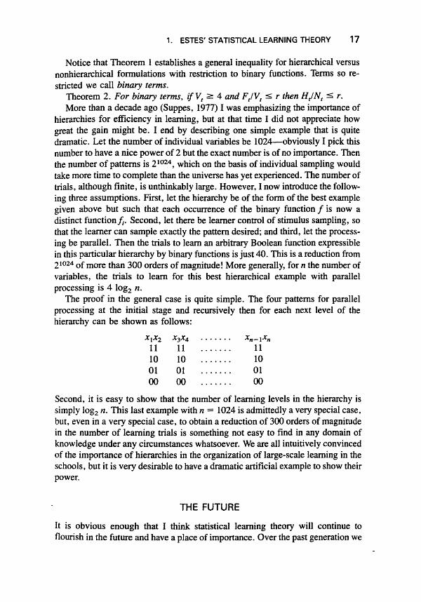
Notice that Theorem l establishes a general inequality for hierarchical versus nonhierarchical formulations with restriction to binary functions. Terms SO re- stricted we call binary terms.

Theorem 2. For binary terms, if Vt 2 4 and FtlVt 5 r then HtINt 5 P. More than a decade ago (Suppes, 1977) I was emphasizing the importance of

hierarchies for efficiency in learning, but at that time I did not appreciate how great the gain might be. I end by describing one simple example that is quite dramatic. Let the number of individual variables be 1024-obviously I pick this number to have a nice power of 2 but the exact number is of no importance. Then the number of patterns is which on the basis of individual sampling would take more time to complete than the universe has yet experienced. The number of trials, although finite, is unthinkably large. However, I now introduce the follow- ing three assumptions. First, let the hierarchy be of the form of the best example given above but such that each occurrence of the binary function f is now a distinct function&. Second, let there be learner control of stimulus sampling, so that the learner can sample exactly the pattern desired; and third, let the process- ing be parallel. Then the trials to learn an arbitrary Boolean function expressible in this particular hierarchy by binary functions is just 40. This is a reduction from

of more than 300 orders of magnitude! More generally, for n the number of variables, the trials to learn for this best hierarchical example with parallel processing is 4 log, n.

The proof in the general case is quite simple. The four patterns for parallel processing at the initial stage and recursively then for each next level of the hierarchy can be shown as follows:

x,x, x3x4 ....... X,- 1%

11 11 ....... 11 10 10 ....... 10 o1 o1 ....... o1 O 0 0 0 ....... O0

Second, it is easy to show that the number of learning levels in the hierarchy is simply log, n. This last example with n = 1024 is admittedly a very special case, but, even in a very special case, to obtain a reduction of 300 orders of magnitude in the number of learning trials is something not easy to find in any domain of knowledge under any circumstances whatsoever. We are all intuitively convinced of the importance of hierarchies in the organization of large-scale learning in the schools, but it is very desirable to have a dramatic artificial example to show their power.

THE FUTURE

It is obvious enough that I think statistical learning theory will continue to flourish in the future and have a place of importance. Over the past generation we

easily be misled into understanding the difficulty of developing it or the usefulness of simplifying abstractions like the pattern model. A pluralism of levels of abstraction and of comesponding models is, in my judgment, a perma- nent feature of any science of complex phenomena. It is naive and mistaken to think we shall find the one true complete theory of learning based on accurate details of how neurons and their connections actually work. Many different levels of theorizing will continue to be of value in many different domains. There is every reason to think that the kinds of applications of statistical learning theory described in the previous section will have a robust future.

More generally, the classical concepts of association, generalization, and discrimination will be extended, but it seems likely that these basic concepts will continue to play the role in the psychology of learning that the concepts of

1. ESTES' STATISTICAL LEARNING THEORY 19

classical mechanics such as force, mass, and acceleration have played for 200 years of physics. It is not that physics has not developed many new concepts and theories, it is, rather, that once fundamental concepts are put in some reasonable mathematical framework and are recognized as having great generality, they do not disappear. Such will be the future of the fundamental ideas of statistical learning theory.

ACKNOWLEDGMENTS

I am grateful to Duncan Luce for a number of helpful comments on an earlier draft.

REFERENCES

Blumer, A.. Ehrenfeucht, A.. Haussler, D., & Warmuth, M. K. (1989). Learnability and the Vapnik-Chervonenkis dimension. Journal of the Assocrarfon for Computrng Machinery, 36, 929- 965.

Bush, R. R., & Mosteller, F. (1951a). A mathematical model for simple learning. Psycholagrcal Review, 58, 313-323.

Bush, R. R., & Mosteller, F. (1951b). A model for stimulus generalization and discrimination. Psyhologrcal Review, 58. 413-423.

Crangle. C.. & Suppes, P. (1987). Context-fixing semantics for instructable robots. Internanonal Journal of Man-Machine Studies, 27, 371-400.

Crangle. C., & Suppes, P. (1990). Introductlon dialogues: Teaching new skills to a robot. Proceed- rngs of the NASA Conference on Space Telerobotics, January 31 -February 2,1989, pp. 9 1 - 10 1.

Estes, W. K. (1950). Toward a statistical theory of learning. Psychological Review, 57, 94- 107. Estes, W. K. (1959). Component and pattern models wlth Markovran interpretations. In R. R. Bush

& W. K. Estes (Eds.), Studies rn mathematrcal leurnrng theory (pp. 9-52). Stanford, CA: Stanford University Press.

Estes. W. K.. & Burke, C. J. (1953). A theory of stimulus vanability m learning. Psychologrcal Revrew. 60, 276-286.

Hllgard. E. R., & Marquis, D. G . (1940). Conditioning und Leurnmg. New York: Appleton- Century

Hull. C. L. (1943). Princrples of Behavior. New York: Appleton-Century. Maas. R.. & Suppes, P. (1985). Natural-language Interface for an instructable robot. Internatronal

Mlller. G. A. (1952). Finite Markov processes in psychology. Psvchologicul Revrew, 17. 149-167 Miller, G. A., & McGill, W. J. (1952). A statistical descnptlon of verbal learning. Psvchometrrka.

Skinner. B. F. (1938). The behavior of organisms. New York: Appleton-Century. Suppes. P. (1959a). A linear model for a contmuum of responses. In R. R. Bush & W. K. Estes

(Eds.), Studies m mathemarm.zl learning theory (pp. 400-414). Stanford, CA: Stanford Univer- sity Press.

Suppes, P. (1959b). Stimulus sampling theory for a continuum of responses. In K. J. Arrow, S . Karlin, & P. Suppes (Eds.). Mathematical methods in the social sciences (pp. 348-365). Stan- ford. CA: Stanford University Press.

Journal of Man-Machine Studies. 22, 215-240.

17. 369-396.