empirical analysis of demand under consumer … analysis of demand under consumer ... this study the...
TRANSCRIPT

UNIVERSITY OF CALIFORNIA DIVISION OF AGRICULTURAL SCIENCES GIANNINI FOUNDATION OF AGRICULTURAL ECONOMICS
Empirical Analysis of Demand Under Consumer Budgeting
Jurg Bieri and Alain de Janvry
Giannini Foundation Monograph Number 30 • Septem.ber 1972
CUG GB930 1-60 (1972)
CALIFORNIA AGRICULTURAL EXPERIMENT STATION
In this study the neoclassical consumer behavior theory and its relation to empirical research in demand are presented in a unified framework. The goal is to make a contribution towards "bridging the gap" between empirical and theoretical demand analysis by generalizing and specializing the theory and extending its applicability to estimation of demand parameters.
The neoclassical theory of consumer behavior and its extension to separable utility functions are treated first. Consumer budgeting as a behavioral justification for separability is then investigated and the concept of stagewise utility maximization is explored in the context of the above neoclassical theory.
Based on this framework, estimation procedures for demand parameters are devised which greatly reduce the amount of empirical information needed to obtain results. An empirical example is provided as an illustration of these procedures.
THE AUTHORS:
Jurg Bieri is Assistant Professor of Agricultural Economics and Assistarit Agricultural Economist in the Experiment Station and on the Giannini Foundation, University of California, Berkeley.
Alain de Janvry is Assistant Professor of Agricultural Economics and Assistant Agricultural Economist in the Experiment Station and on the Giannini Foundation, University of California, Berkeley.

CONTENTS
I. Introduction and Summary . 3 II. Neoclassical Demand Theory 5
III. Separable Utility Functions . 13 Weak Separability . . 13 Strong Separability . . 14 Pointwise Separability . 15 Pearce Separability 15 Block-Additivity . . . 15 Gossen Additivity 16
IV. Estimation of Demand Parameters Under Separability: A Review . . . . • . 16
V. Budgeting and Recursive Systems of Demand Equations . . . . . . . . . . . . 20
VI. Determination of Local Group Prices Indexes Under Strong and Weak Separability . 22
VII. Estimation of Price and Income Slopes and Forcasting Under Strong and Weak Separability 26
VIII. Estimation of Price and Income Slopes Under Separability into Homogeneous Subfunctions and Under the Composite Goods Theorem . 29
IX. A proposal for Stepwise Forecasting . . 32 X. Estimation of Demand Parameters with a
Quadratic Utility Function . . . . . 35 XI. Partitions of the Commodity Space . . 39
Testing Whether a Given Partition is Strongly
Discovering a Partition and the Nature of Its Separable . . . . . . . . 39
Separability . . . . . . . . . . . 40 Cluster Analysis of Demand . . . . . 42
XII. Estimation of the Flexibility of Money and International Comparisons . . . . . . 43
XIII. Estimation of Expenditure Functions for Major Categories of Items. . . . . . . . . . 47
XIV. Estimation of Second-Stage and Two-Stage Demand Parameters . 49 Glossary of Symbols . 55 Literature Cited . . 57
jurg Bieri and Alain de Janvry
EMPIRICAL ANALYSIS OF DEMAND UNDER CONSUMER BUDGETING1
I. INTRODUCTION AND SUMMARY
DETAILED KNOWLEDGE of the magnitude of price and income elasticities of con sumer demand is essential for decision-making in both free and planned market economies. In spite of their importance, few elasticities have been estimated in the context of complete systems of demand equations deriving consistently from utility theory. This deficiency results from a prevalent "gap between theory and empirical analysis" (Houthakker, 1960a) of consumer behavior. This gap arises from the fact that the neo-classical theory provides an insufficient basis for empirical analysis because of the weakness of its restriction on behavior and that the factual confrontation of its postulates or of its derived hypotheses is a near impossibility as discussed by Clarkson (1963) and Mishan (1961).2 As a result, many econometricians, desirous to evaluate the demand for consumer goods, start their analyses by deciding that " ... it would, therefore, be a mistake to impose the a priori considerations of this theory on the assumptions of our statistical analysis" (Cramer, 1962, p. 1). The same difficulty is found in many fields of economic analysis. Samuelson (1947, pp. 3 and 4) noted that"... only the smallest fraction of economic writings, theoretical and applied, has been concerned with the derivation of operationally meaningful theorems," where "by meaningful theorem, I mean simply a hypothesis about empirical data which could conceivably be refuted, if only under ideal conditions."
Three distinct but complementary courses of action can be followed to cope with this gap between theory and empiricism, which is essentially a problem of degrees of freedom (de Janvry and Bieri, 1969). First, the theory of consumer behavior can be modified, both by specializing it through further specification of the structural model and by generalizing it through broadening the context of application of the model to allow for intertemporal and interpersonal comparisons (Houthakker; 1960a; Papandreou, 1958). These extensions of theory aim at providing systems. of demand equations which are adequate for statistical estimation. Secondly, the data base can be extended, both in the temporal and cross-sectional dimensions, for ex,. ample, through consumer panel surveys. Thirdly, statistiCal methods can be im,.. proved to deal with specification errors in linear models, particularly multieolli~
1 Submitted for publication May, 1972. 2 See, nevertheless, the tests of Koo (1963) and Dobell (1965} on the consistency of eon··
sumer choices using revealed preferences and of Barten (1967) on the symmetry of the Slutsky substitution terms matrix. Both tests only provide weak evidence because the ideal conditions of the model are not met in the data.
[3]

4 Bieri and de J anvry: Empirical .Analysis of Demand
nearity and serial correlation, and with nonlinear estimation. In the present study all three approaches are followed, but main emphasis is given to theoretical extensions.
The additional behavioral assumption of stepwise decision-making resulting from the budgeting of consumer expenditures ala Strotz (1959, 1957) and Gorman (1959) is imposed on the neoclassical model. The objective of the present study is to render this extended model amenable to measurement and, in this fashion, of contributing toward a methodology for bridging the gap between theory and empirical analysis of demand.
In section II a synthesis of the neoclassical theory of consumer behavior is presented for the purpose of deriving the restrictions it imposes on the parameters of demand equations. The definitions of different types of separability are given in section III in terms of the restrictions they impose on the utility function as well as on the price elasticities. Section IV reviews previous applications of the separability assumption to empirical analysis. Four categories of utilizations are distinguished. The first consists of imposing the separability hypothesis directly on the utility function, the second and third of introducing the restrictions implied by separability in the demand functions or their total differentials, and the fourth of using the relationships among demand parameters implied by separability to derive additional parameters from a set of known ones.
The implications of the budgeting hypothesis on the estimation of systems of demand equations are investigated in section V. Budgeting implies a stepwise maximization of a separable utility function according to which income is allocated first to budget categories, and then the optimal levels of commodity demand within each group are determined. Under reasonable assumptions about the stochastization of the first-stage expenditure functions and the second-stage demand functions, the latter can be .estimated independently because the system as a whole is then recursive. By contrast to the demand functions obtained from the neoclassical model, each second-stage demand function contains only as many parameters as there are items in the budget category, plus one for the group expenditure variable. As a result, the time series data requirements are limited to prices of items in the budget category and to group expenditure. For this budgeting procedure to be efficient in simplifying the consumer's decision process without loss of utility, price indexes, at least in differential form, need exist. In section VI the existence of local i13dexes under strong separability is proven, and their functional form is given. A similar derivation shows that, under weak separability, a whole matrix, rather than a vector, of local price indexes is now required.
The relationships between second-stage and two-stage (overall) income and price slopes are established in section VIII under strong separability. The factors needed to correct the second-stage slopes are functions of elements which are either directly observable or estimable from cross-section information, except for one parameter which is proportional to the marginal utility of income. An estimation procedure for this parameter, based on cross-section data at two points in time, is made explicit.
In the next section it is shown that global group price indexes exist if the utility function is separable into homogeneous subfunctions or if Hicks' theorem on composite goods holds (Hicks, 1939). After deriving the functional form of these price indexes and the corresponding quantity indexes, the expenditure functions, as well
5 Giannilni Founda,tion Monogra,p·h • Number 30 • September, 197$
as the second-stage and two-stage income and price slopes, are obtained under perfect aggregation. Although short-run forecasts of group expenditures can be obtained under local aggregation using the total differential of the expenditure functions, long-run forecasts require the existence of global allocation functions. Because' of the stringent conditions for their existence, a compromise is suggested in section IX. Global functions are used to predict group expenditure, but secondstage demand functions are then estimated under strong separability only. The resulting specification error is analyzed.
Because of the need of having demand equations, which are easily amenable to statistical estimation and are derived from a nonseparable utility function for the measurement of second-stage demand parameters, the quadratic utility function is considered in section X. After presenting the properties of this function, two methods for estimating the demand parameters are developed. The first is based on an orthogonal regression technique and the second on a linearization of the demand equations.
Direct tests or empirical determination of partitions are possible and provide an empirical foundation for the hypothesis of separability. Several methods are proposed in section XI for testing or finding budgeting categories. These procedures are based on cross-sections at one or two points in time or on previous estimates of price and income elasticities. Partial empirical evidence tends to confirm the separability between the food and nonfood items, also the existence of some groupings within the food category.
The flexibility of money is a key variable in the estimation of demand parameters with consumer budgeting because it enters into the equations establishing a correspondence between second-stage and two-stage elasticities. It constitutes, in addition, a practical although restrictive cardinal indicator of welfare because it is a transformation of the marginal utility of income (Goldberger, 1967b). A number of values of the flexibility of money, obtained from the literature, are related functionally to income and prices. Predictions based on an empirical fit of this function can then be calculated.
The methodology for the empirical analysis of demand under consumer budgeting developed in this study is illustrated in the last two sections with Argentine data. Expenditure functions are estimated in section XIII. They permit the determination of changes in group expenditures due to percentage changes in the price of individual items aµd in income. In section XIV, second-stage demand elasticities are measured and transformed into two-stage elasticities.
II. NEOCLASSICAL DEMAND THEORY
Let U (q1, ••• , ~T; a1, ..• , aT) be an individual consumer's intertemporal utility function, assumed to be at least twice differentiable, where qi (qu ... q,,,,) is an n-dimensional vector of quantities demanded in period t, at is a vector of parameters, and Tis the, consumer's planning horizon.3 Under the assumption of "weak time perspective/' which implies some restrictions on the complementarity between consumption in the different time periods, Koopmans, Diamond, and Williamson
3 A glossary of symbols is given on page 55.

6 Bieri and de Jarvvry: Empirical .cl.nalysis of Demand
(1964) have shown that the intertemporal utility function U can be rewritten in the separable form
where Vis continuous and increasing in u and U1·u is the instantaneous utility, while U1 is the aggregate utility function of the consumption program that starts with the second period, evaluated as if it were to start immediately. The consumer
T
is assumed to maximize V, subject to a budget constraint L '!ftqt = Y, where Y is t-1
the present value of the stream of disposable income and Pt the vector of discounted prices in period t. He will follow in this fashion a "naive optimum path" (Blackorby, 1968) where the optimum intertemporal allocation of expenditures is determined through a new maximization at each point in time.4
Let us assume that the consumer has been able to allocate his income over present and future consumption programs-a decision process we shall make explicit later.6 If m is the income allocated to the first period, the problem then reduces to the maximization of the instantaneous utility under the constraint that p'q = m (for simplicity, the time indexes are henceforth omitted). The objective function is, hence, to maximize, with respect to q and X,
u(q, a) - X(p'q - m) (1)
where X is a Lagrange multiplier. The first-order conditions for a maximum of utility are:
uq(q, a) - Xp 0 (2)
p'q-m=06
where uq(q, a) is an n-coordinate vector of marginal utilities, iJu~q,q;
a) , i = 1, ... , n.
The second-order conditions are:
> 0 for all i 1, ... , n (3)(-1)'
, 0
where H(i)(•) is the principal minor of order i of the symmetric Hessian matrix H with characteristic element iJ2u(q, a)/iJq;iJq;(i,j = 1, ... , n)1 and where P<i) is the
4 This decision strategy is of an "open loop" nature and is thus generally suboptimal for a multiperiod optimization.
• A similar procedure to the budgeting described in section IX for allocating income to groups within a single period can also be used to distribute the present value of the stream of all future disposable income between instantaneous and future consumption programs.
6 A more general formulation would be obtained in a nonlinear programming framework with p'q - m ;;:;:; 0, q '1;; O. Thia latter formulation properly characterizes the corner solutions while the neoclassical formulation used does not.
7 Throughout the text when characterizing elements of matrices, the first index refers to rows and the second to columns.

1 Gian11Mli Founilation Monograph • Number 80 • September, 1972
corresponding vector of i elements of p. When i =n, the matrix H bordered by price vectors, as in equation (3), is the "bordered Hessian matrix." Equations (2) and (3) constitute the structural form of the model.
If we let the parameters a be functions of a set of s exogenous variables z that characterize the consumer (his social, familial, and individual characteristics-in particular, his habits), the reduced form of the model is:
q = q(p, m, z) (4)
).. = X(p, m, z).
The first n equations are the demand equations which span an (n - 1) dimensional space since any nth quantity can be obtained from the (n - I) others through the budget constraint.
To derive the restrictions implied by the model on the parameters of the demand functions, we take the total differential of the system of reduced-form equations:
(5)
where
Q an n X n matrix of Cournot price slopes iJqifiJp1 q,,. = an n-coordinate vector of income slopes aqi/am Qz = an n X s matrix of elements aq.;/iJZ; Ap =an n-coordinate vector of elements fJX/iJp; Xm =ax/am
and
X, = an s-coordinate vector of elements iJX/aZi.
Taking similarly the total differential of the system of first-order conditions, we get
H -pJ [dq] = [Xln 0 (6)
[ -p' 0 dX q' -1
where Uqz is an n X s matrix of elements iJU;/iJzil and In is an identity matrix of size n. This system can be solved for dq and dX since the inverse of the bordered Hessian exists according to (3). Equating the expressions obtained for dq and dX in the systems of equations (5) and (6), we get the "fundamental equations" (Theil, 1965; Barten, 1964):

8 Bieri aniJ, iJ,e J anvry: Enwir·ioai Analysis of Demand
qm -p 0Q'] [ H r[H• -u.J (7)A~ = -p'[~; Am 0 q' -1 O'
or
QJ [B :.J [H" -u.J (8)[~; qm 0
A' = b'Am q' -1 O'
where we defined
(9)[_:, -:J [:, :J [~· :J The fundamental equations (8) and (9) imply the following restrictions on de
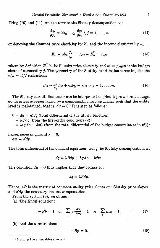
mand parameters. From the system (8), we obtain: (a) The Slutsky decomposition of the price slopes
Q =AB+ bq' (10)
where AB is the matrix of Slutsky substitution terms Ab;1(i, j 1, ... , n) and bq' is the matrix of income effects b;q1(i, j = 1, ... , n). The second-order conditions and the symmetry of the Hessian matrix imply that B is symmetric, negative semidefinite.8 All the cross-price substitution effects are, hence, symmetrical, Ab;; = Ab1,(i r6 j = 1, ... , n), and the own-price substitution effects Abii(i = 1, ... , n) are negative or zero.
(b) Two definitions
aq., b' 1- b or am = - ; i = , ... ,n (11)
and Am= -bo• (12)
(c) The decomposition of the price slope of the marginal utility of income
, (13)
(d) The Tintner-Ichimura equations (Basmann, 1956, p. 51)
Q. = -BUqz·
s If D is the determinant of the bordered Hessian matrix, D;; the cofactor of its (i, j)th element, and D;. of its (i, n + l)st element, the Slutsky decomposition of price slopes is:
i'Jq; X D,; + D,. . i'Jp; D D q,.
Symmetry of H implies that D;; D;; and, hence, that XB is symmetric. The second-order conditions imply that D., and Dare of opposite signs and, hence, that all the diagonal elements of XB are negative or zero since X is always nonnegative.
9 Gia'lll/1,ini FO'Unilation Monograph • Number 30 • Septemb·er, 1972
Using (10) and (11), we can rewrite the Slutsky decomposition as:
aq, "b aq, . . 1,,.-- = I\ ;,; - q; ,,.-- i, J = , ... ,n (14)up; um
or denoting the Cournot price elasticity by E•; and the income elasticity by ·ru,
(15)
where by definition E,; is the Slutsky price elasticity and w; p;q;/m is the budget share of commodity j. The symmetry of the Slutsky substitution terms implies the n( n - 1)/2 restrictions
E,; = w; E;; + w;(11; - ,,,,)i ;>!! j = 1, ... , n. (16)w,
The Slutsky substitution terms can be interpreted as price slopes where a change, dp, in prices is accompanied by a compensating income change such that the utility level is maintained, that is, du= 0.9 It is seen as follows:
0 = du = u~dq (total differential of the utility function) = "Ap'dq (from the first-order conditions (2)) = "A(q'dp - dm) (from the total differential of the budget constraint as in (6));
hence, since in general "A ;>!! 0, dm = q'dp.
The total differential of the demand equations, using the Slutsky decomposition, is:
dq "ABdp + bq'dp - bdm.
The condition du = 0 thus implies that they reduce to:
dq = "ABdp.
Hence, AB is the matrix of constant utility price slopes or "Slutsky price slopes" and q'dp the necessary income compensation.
From the system (9), we obtain: (a) The Engel equation:
-p'b = 1 or Lp, iJq,. = 1 or (17) i am
(b) and then restrictions
-Bp = 0. (18)
9 Holding the z variables constant.
10 Bieri and de Jar11Vry: Empir·ical Analysis of Demand
Premultiplying (IO) by p and using equations (17) and (18), we get the Cournot aggregation equation
'Q I '"' (}qip = -q or L...J pi- -q; or L w;,Eii -w1 j = 1, ... , n. (19)i ()pj i
An alternative form of the same restriction is obtained by postmultiplying (10) by p which gives
aq, '°'E . 1Qp = bm or L ~qi Pi ~m or L...J if= -ru i = , ... , n. (20)i vpj um i
Further properties of the demand functions are their uniqueness and their homogeneity of degree zero in prices and income. The first property derives from the differentability of the utility function and the nonvanishing Jacobian of the transformation (implied by the second-order conditions) which guarantee a unique solution to the system of structural equations. The second property derives from the budget constraint which is homogeneous of degree zero in p and m.
Applying Euler's theorem to the demand equations provides a set of n restrictions on the demand parameters, known as the Euler aggregation equations:
0 or L aq; Pi + aq; m 0 or i ap1 am (21)
I: 'f/i = o i = 1, ... , n. i
But these restrictions are not independent of the Slutsky and Cournot aggregation equations since they can be derived from (10), (17), and (18) and are identical to (20).
Making an account of the number of independent restrictions among demand parameters, the properties of the matrix of Slutsky substitution terms imply
n2
---n
restrictions (in(n 1) symmetry restrictions on the off-diagonal terms
and n negativity restrictions on the diagonal terms); the Engel aggregation equation implies one restriction; and either the Cournot aggregation, the Euler aggregation, or.1..~quations (18) imply another n restrictions.
·Using equations (2) and (17),
au -u~b = -A.p'b =A..
am
Hence, A. is the marginal utility of income. The elasticity of A. with respect to income has been called by Frisch (1959) the "money flexibility,"~ A.mm/A.. Being a function of A., ;;; is a function of prices and income.
Since, from (12) and (9), Am bo = -IHl/D where D is the determinant of the bordered Hessian matrix, IHI ¢ 0 if A.m ¢ 0, that is, if the marginal utility of income is not independent of income. The Hessian matrix then has an inverse, and we can express B, band bo in terms of H-1 as:

11 Giannini Foundation Monograph • Number 30 • September, 1972
(22)
(23)
(24)
The price slopes are hence decomposed further than in (10) into
Q = xn-1 - (A/'Am)bb' + bq'. (25)
The total differential of the demand equations, using the decomposition of equation (25) due to Frisch (1959, p. 184), becomes
dq = AH-1dp - b (~m b' - q') dp - bdm. (26)
The matrix of Slutsky substitution terms is separated in an additive fashion into a matrix of "specific" substitution effects, AH-1, and a matrix of "general" substitution effects ('r./'Am)bb'.
The specific substitution terms can be interpreted as price slopes where a change dp in prices is accompanied by a compensatory income change such that the level of the marginal utility of money is maintained, that is, d'r. = 0.10 This can be seen as follows:
0 = d'r. = 'r.~dp Amdm (from (5))
Ab'dp - Amq'dp + Amdm (from (8)).
Hence, dm = -[('A/'Am)b' - q'Jdp.
Thus, to recapitulate:
Q is the matrix of usual Cournot price slopes where money income is held constant.
'AB is the matrix of income compensated or Slutsky price slopes with constant utility.
xH-1 is the matrix of income compensated or Frisch price slopes with constant marginal utility of income (MUM).
q'dp is the income compensation to maintain utility constant.
( - :m b' q') dp is the income compensation to maintain the MUM constant.
Frisch's decomposition can be rewritten in terms of elasticities by premultiplying (25) by D-;;1 and postmultiplying it by D:P where D,, denotes the diagonal matrix whose elements are the arguments of the vector x:
io Holding the z variables fixed.
12 Bieri and de Jarvvry: Empirical Analysis of Demand
E = E** - +rir/Dw - riw', (27) ml\m
while in similar notation the Slutsky decomposition in (15) is
E = E* - 1JW1• (28)
In these equations E is the Cournot price elasticity matrix with constant money income, E* the Slutsky price elasticity matrix with constant utility, E** the Frisch price elasticity matrix with constant MUM, 11 is the vector of income elasticities, and w the vector of budget shares.
A slightly stronger specification of the utility function is to assume that H is negative definite. The second-order conditions are then necessarily satisfied since
holds for all i. The following additional properties are also obtained:
U;; < 0 all i = 1, ... , n.
The indirect utility function, first introduced by Hotelling (1932) and investigated extensively more recently by Samuelson (1965), is a function of prices and income that gives the maximum value of utility for each price and income situation. It thus constitutes an ideal welfare indicator. It can be written as u[q0 (p, m)] = v(p, m) where q0 is the maximizing value of q. The partial derivatives of v(p, m) with respect to m and p are:
av f aqoam = Uq am = - Xp'b = A.
Hence, again, X is the marginal utility of income.
' (av)' ,Q " 'Q " , nap = Uq = "p = - "q. (29)
- l av h d d t· · 1. · fHence, q = T ap are t e eman equa 10ns m exp wit orm.
The indirect utility function can be solved uniquely for the expenditure function
m = m(u, p).
11 Roy identity (1943).

13 Giannmi Foundation Monograp·h • Number :!JO • September, 1972
It gives the minimum income level necessary to obtain the level of utility u when prices are p.
The price and utility slopes of the expenditure function are: am/iJp = q(u, p), the Hicksian demand equations in explicit form; and iJm/iJu l/f.., the reciprocal of the marginal utility of income. The expenditure function permits defining the true cost-of-living index P between two price situations po and P1 where the level of utility is maintained constant,
P = m(u, p1)/m(u, po).
III. SEPARABLE UTILITY FUNCTIONS
The demand equations derived from the neoclassical theory are generally not amenable to econometric analysis because of the large number of independent parameters entering these equations. The length of the time series available on consumer behavior is usually short relative to the number of items that enter into the consumer's budget, and the problem is further complicated by multicollinearity among price series. This problem of degrees of freedom which is common to many areas of economic analysis can be dealt with using three distinct complementary approaches. One is the specialization of the theoretical model through additional behavioral postulates in order to reduce the number of independent parameters. Another is the extension of the data base, in particular through the combination of time series and cross-section observations. The third is the development of more efficient estimation methods, in particular to cope with the problem of multicollinearity. All three approaches are used in this monograph.
Further restrictions on the neoclassical model of consumer choice have been introduced by Leontief (1947) and Sono (1961) through the assumption of separability of the utility function.
Consider a partition of the set of n commodities into S mutually exclusive and exhaustive subsets (groups) of sizes nR(R =I, ... , S). The idea of separability consists of specifying that the ratio of the marginal utilities of a pair of commodities r and s is not affected by the quantity consumed of a third commodity k. Hence, if u,. denotes the marginal utility of item r, rands are separable from kif
Several types of separability have been defined according to the respective groups to which commodities r, s, and k belong.
Weak Separability
Under weak separability, commodities r and s are in the same group, while k belongs to another group:
iJ(u,/u/)/iJq1o = 0 for all r, r'dl; ktR. (30)
14 Bieri and de Jawvry: Empir.foal .Analysis of Demand
The corresponding utility function is of the form
u(q) F[fr(qr11 • • • , qr ) , · · · , f s(qs1, • • • , qs )], (31)"'r ns
and the Slutsky substitution terms are
(32)
(JRK is a proportionality parameter that is a function of prices and income. Equati.ons (32) and (18) imply that the own-price Slutsky substitution term is of the form
(33)
Goldman and Uzawa (1964) have shown that equations (30), (31), and (32) can be taken as equivalent definitions of weak separability.
Strong Separability
Under strong separability, commodity k belongs to a group that does not contain r and s, while these two commodities may or may not be in the same group:
iJ(ur/u.)/iJqk 0 for all kfK; r, s ~ k. (34)
Hence, when r and s belong to the same group, strong separability reduces to weak separability.
The corresponding utility function is of the form
u(q) = F[fr(q11, .. ·,qr ) + · · · + fs(qs1, • · ·, qs )] ' (35)"r "s
and the Slutsky substitution terms are
(36)
, (37)
where the proportionality parameter 6, while still a function of prices and income, is now independent of the groups concerned. Again, equations (35), (36), and (37) can be taken as equivalent definitions of strong separability.
Pointwise Separability
If there is only one commodity in each group, strong separability reduces to pointwise separability
iJ(u,/u;)/iJq,. = 0 for all i, j, k = 1, ... , r. (38)
15 Giannini Foundation Monograph • Niimber 30 • September, 1972
The corresponding utility function is of the form
(39)
and the Slutsky substitution terms are
for all i ~ j = 1, ... , n (40)
(41)
Pearce Separability
If, in addition to weak separability between groups, commodities are point-wise separable within each group, the partition is Pearce separable (1964) and
for all r, r'eR; k ~ r, r'. (42)
The corresponding utility function is of the form
and the Slutsky substitution terms are
(44)
r, r'eR (45)
(46)
Two cardinal versions of strong and pointwise separability are, respectively:
Block-Additivity
Under block-additivity, 'I.ti;= 0 for all id, jEJ ~I, where u,1 is the (i, j)th element of the Hessian matrix which is, hence, block-additive. Thus, while under separability ratios of marginal utilities are independent of certain quantities consumed, under additivity this independence applies directly to the marginal utilities.
The corresponding utility function is
u(q) = f1(q11' ... , qr ) + ... + fs(qs11 .. . , qs ). (47)nl ns
The Slutsky substitution terms are the same as those under strong separability where (} takes on the particular value
v (} = -"X/Xm = -m/w (48)

16 Bieri and de Jarvvry: Empirical Analysis of Demand
since the specific substitution term in Frisch's decomposition (25) vanishes for items in different groups.
Gossen Additivity
Gossen additivity is the case, of pointwise block-additivity, hence, of a diagonal Hessian matrix. The Slutsky substitution terms are the same as those under pointwise separability with fl -m/:f.
Note that additivity can be specified with a utility function that is only twice differentiable as, for example, the quadratic while strong, weak, or Pearce separability requires the utility function to be at least thrice differentiable.
Pointwise additivity implies severe restrictions on the substitutability and complementarity between commodities. Green (1961) has shown that in this case either (1) all goods are normal and substitutes for each other or (2) one good is normal and a substitute for all other goods which, in turn, are either inferior and complements to each other or neutral and unrelated to each other. Pointwise additivity thus seems to be acceptable only when applied to the quantity indexes of major categories of items in which case (1) above is likely to be satisfied. For this reason, Pearce separability appears to be a rather implausible specification of the utility function. But use of pointwise additivity then requires the existence of quantity and price indexes for these major categories of items. As we shall see later, existence of such indexes (which require either separability into homogeneous subfunctions or Hicks' theorem (1939)) is empirically doubtful.
IV. ESTIMATION OF DEMAND PARAMETERS UNDER SEPARABILITY: A REVIEW
The hypothesis of separability has been widely used in the empirical analysis of consumer demand for the purpose of reducing the number of independent parameters in the equations to be fitted. We can categorize as follows the ways in which it has been utilized:
1. The functional form of separable utility function is completely specified. Demand functions can then be derived explicitly and estimated. The functional forms of utility that have been used for empirical analysis imply Gossen or blockad,titivity, with the exception of the quadratic (Bieri and de Janvry, 1971a).
Under Gossen additivity, the ratio of the price elasticities of any two items with respect to a third one is equal to the ration of their income elasticities. Houthakker's (1960a) "direct addilog,"
u(q) = L n
a,,r/f,i, 0 < f3i < 1, a; > 0, La;= 1, i-1 i
is in this category and implies further that ratios between income elasticities are constant. The "Stone-Geary" (Stone, 1954; Geary, 1949-50; Parks, 1969; Goldberger, 1967a; and Powell, 1966),
17 Giannini Foundation Monograph • Number 30 • September, 1972
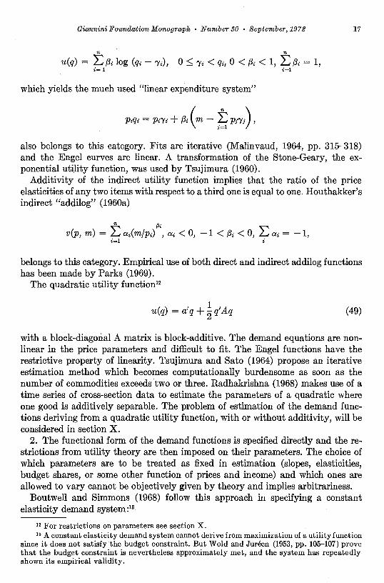
u(q) = :t f3i log (qi - 'Yi), 0 ::; 'Yi < qi, 0 < f3i < 1, :t {3; = 1, i= I i=l
which yields the much used "linear expenditure system"
p;qi = Pi'Yi + {3; (m - t Pi'Yi), 1~1
also belongs to this category. Fits are iterative (Malinvaud, 1964, pp. 315-318) and the Engel curves are linear. A transformation of the Stone-Geary, the exponential utility function, was used by Tsujimura (1960).
Additivity of the indirect utility function implies that the ratio of the price elasticities of any two items with respect to a third one is equal to one. Houthakker's indirect "addilog" (1960a)
n {3;
v(p, m) = L ai(m/pi) , ai < 0, -1 < f3i < 0, La; = -1, ~l i
belongs to this category. Empirical use of both direct and indirect addilog functions has been made by Parks (1969).
The quadratic utility function12
u(q) = a'q + 1 q1Aq (49)
2
with a block-diagonal A matrix is block-additive. The demand equations are nonlinear in the price parameters and difficult to fit. The Engel functions have the restrictive property of linearity. Tsujimura and Sato (1964) propose an iterative estimation method which becomes computationally burdensome as soon as the number of commodities exceeds two or three. Radhakrishna (1968) makes use of a time series of cross-section data to estimate the parameters of a quadratic where one good is additively separable. The problem of estimation of the demand functions deriving from a quadratic utility function, with or without additivity, will be considered in section X.
2. The functional form of the demand functions is specified directly and the restrictions from utility theory are then imposed on their parameters. The choice of which parameters are to be treated as fixed in estimation (slopes, elasticities, budget shares, or some other function of prices and income) and which ones are allowed to vary cannot be objectively given by theory and implies arbitrariness.
Boutwell and Simmons (1968) follow this approach in specifying a constant elasticity demand system :13
12 For restrictions on parameters see section X. 13 A constant elasticity demand system cannot derive from maximization of a utility function
since it does not satisfy the budget constraint. But Wold and Jureen (1953, pp. 105-107) prove that the budget constraint is nevertheless approximately met, and the system has repeatedly shown its empirical validity.

18 Bieri and de J anv1·y: Empfr.ieal AnaJysis of Demand
log q a + E log p + 17 log m. (50)
Assuming strong separability and using the Slutsky, Cournot, and Engel aggregation equations, the equations of (50) reduce to
log qr = ll!r + .?: .Brr'(log Pr' log Pr)+ !_11r LL 'l]k m K""R k
r ""'' (51)
[w"(log Pk - log Pr)] - 11r (2: L Wk log Pk log m), nR K k
where wk = pkqk/m denotes the budget shares and .Brr'
treated as fixed parameters. Because the income elasticities enter in two regression parameters and the re
striction that this imposes among regression coefficients is nonlinear, estimation of the system is iterative. The procedure is computationally cumbersome, has no known convergence, and does not provide knowledge of the statistical properties of the estimates obtained. The number of coefficients to be estimated in each equation is reduced from n in the neoclassical model to nR 1, yet the iteration has to be performed over the whole system of n equations. Byron (1970) proposes a method to estimate the constant elasticity demand system subject to the parameters satisfying the nonlinear restrictions imposed by the separability hypothesis.
Powell (1966) starts with a linear expenditure system and imposes the implied additivity restrictions only at the mean price and quantity levels. Fits are again iterative. Goldberger (1967b, pp. 95~101) shows that Powell's formulation is essentially identical to the one deriving from a Stone-Geary.
3. The hypothesis of separability can be introduced in the context of total differentials of the demand functions. This is the approach followed in the "Rotterdam School" by Theil (1965, 1967b), Barten (1969, 1967, 1968), Barten and Turnovsky (1966), and Parks (1969). It has the advantage of not requiring specification of the demand functions and of being linear in the price and income slopes which permits an easy imposition of the theoretical restrictions on these slopes. The total differential of the system of demand equations, presumably taken at some eguilibrium point in the center of the observed scatter of points, is, using the ~utsky decomposition (10), dp A.Bdp - qmq'dp qmdm, or, using the identities dp = D.d log q where D. is a diagonal matrix of elements q, dp = E*d log p 17w1d log p + 17d log m where E* D-;1 A.BDP is the matrix of constant utility price elasticities and w the vector of budget shares. Multiplying each equation by the corresponding budget shares, we get the system
Dwd log q = DwE*d log p + Dw11[d log m w'd log p]. (52)
Approximating the differentials by first differences, Barten (1967) estimates this system treating DwE* and Dw11 (the "marginal budget shares") as fixed parameters. Decomposing further E*, using Frisch's decomposition (25), into

19 Giannini Foundation Monograph • Niimber 30 • September, 1972
D* = E** - lriri'Dw v w
where E** = n-;;1'xH-1DP is the matrix of MUM compensated price elasticities, Theil (1965, 1967a) estimates the system
Dwd log q = DwE**d log p _ l (Dwriri'Dwd log p)v w
(53) + Dwri(d log m - w'd log p).
The estimable parameters are now DwE**, ~' and Dwri· Estimation is iterative because the unknown income elasticities enter into the definition of the variable attached to the flexibility of money. Under block-additivity (Barten, 1964), the system becomes, using (36) and (37),
w,d log q, = L w,E~'(d log Pr' - d log p,) _ l W,rJ, L L ,',.,, i:, K"'R T
(54) [wkT/k(d log Pk - d log p,)] + w,ri,(d log m - w'd log p), all rtR.
Estimable parameters are as before, but the number has decreased from n + 1 in (52) and n + 2 in (53) to nn + 1. Again, estimation is iterative unless the income elasticities are known a priori. In most cases, the Rotterdam model has been estimated under Gossen additivity (Theil, 1965, 1967a), in which case (53) reduces to the simple expression
IDwd log q= -1 DwD 71 (I -IrJrir1Dw) dlog p + Dwri(d log m - w 'd log p)v
w v (55)
where wand Dw'YJ are estimated by iterating.
Major difficulties with the Rotterdam School approach are:
(a) The equation fitted has local validity only since it is the tangent hyperplane to the demand surface at one equilibrium point. The approximation may be quite poor if the range of variation of the data is large and the true demand curves not approximately linear.
(b) Approximating differentials by first differences creates a problem of specification error which is all the worse as the true demand equations depart more from linearity.
(c) The choice of the parameters to be treated as fixed in the estimation remains arbitrary.
(d) The iterative estimation system followed is cumbersome, has no known convergence properties, and has no distribution theory for the resulting estimates.
Goldberger (1969) has shown that, if the model (55) with Gossen additivity and constant marginal budget shares were to hold in the large, it could be derived from
20 Bieri and de J anvry: Empir·ical .Analysis of Demand
a Stone-Geary utility function. In that case we could use directly the equations of the linear expenditure system instead of equations in differential form.
4. The relationships among parameters implied by separability are used directly to derive additional parameters from a set of known ones. Johansen (1964) and Amundsen (1964) use the Gossen additivity assumption to derive all direct and cross-price elasticities from the knowledge of the income elasticities and of either the money flexibility~ or of one price elasticity in (41). Brandow (1961) and George and King (1971) use the assumption of block-additivity to estimate the cross-price elasticities between food and nonfood items.
V. BUDGETING AND RECURSIVE SYSTEMS OF DEMAND EQUATIONS
We saw that separability has been used in the empirical analysis of consumer demand as a way of obtaining further restrictions on price and income slopes and of thus reducing the number of independent parameters to be estimated. Justification for the introduction of the separability hypothesis in the classical model of consumer behavior was based upon the property of independence of certain ratios of marginal utilities between pairs of items with respect to the quantities demanded of other items.
Strotz (1957, 1959) and Gorman (1959) propose a very appealing behavioral interpretation of the separability property in terms of budgeting of the consumer's expenses over groups of commodities as a simplifying process in decision-making. With budgeting, maximization of the utility function takes place in stages, say, two for simplicity. In the first stage, income is allocated to a set of S(R = I, ... , S) groups of commodities or budget categories. In the second stage, each group expenditure mR, determined in the first stage, is allocated to the nR(r = 1, ... , nR) individual items in group R.
The first-stage group expenditure equations are:
s mR = mR(Pr, ... , Ps, m), R = I, ... , S, with L mR = m (56)
R-I
where PR = PR(PR1, • •• , PR ), R = I, ... , S, are group price indexes (which,nR
fc.tr the time being, are assumed to exist) that are functions only of prices in the corresponding group. The second-stage demand equations are:
The demand equations for individual commodities after maximization in two stages, which we shall call the "two-stage demand equations," are consequently
Thus, the two-stage price and income slopes are, respectively,
21 Giannim,i Foundation Monograph • Number 30 • September, 1972
( aq, ) + aq, amR r r' eR 1 (58)
ap,' mR amR aPR ap,' '
where the symbol ( )mR indicates that mR has been held constant in the process of
differentiation,
aq,-8
-mR
amR aPK::ip -
8-, reR, keK ;;r; R
v K Pk (59)
and
aq, am
= aq, iJmR
amR . iJm
(60)
To the three definitions of price slopes introduced in section II, namely, (I) the Cournot price slopes where money income is held constant, (2) the Slutsky price slopes where utility is held constant, and (3) the Frisch price slopes where the marginal utility of income is held constant, we are, hence, now adding a fourth definition-(aq,/ap,r)mR-the second-stage Cournot price slopes where group ex
penditure is held constant. Just as in the Cournot price slopes, these second-stage Cournot price slopes can be
further decomposed into: (I) second-stage Slutsky price slopes where the group utility fR (.) in the utility function is held constant and (2) second-stage Frisch price slopes where the marginal utility of expenditure on group R, f...R, is held constant.
Since mR is determined in a first-stage maximization, it is predetermined with respect to q,, and the system of first- and second-stage demand equations is blockrecursive. One block is composed of the first-stage expenditure equations and the other of the second-stage demand equations. If we assume that random disturbances are introduced in these equations to account for errors in maximizing, the variancecovariance matrix of residuals will be block-diagonal since maximization is performed in two separate stages. Thus, the second-stage demand equations can be fitted independently of the first-stage expenditure functions. Further, second-stage maximization takes place separately in each budget category so that errors in maximizing cannot be transmitted from one group to another. The variancecovariance matrix of the system of second-stage demand equations is, hence, also block-diagonal, and each of the S systems of equations can be fitted separately. Within each of these systems, all the exogenous variables are the same-namely, PR1, ... , PR , mR-SO that, following Zellner (1962), consistent and efficient esti
"R mates can be derived from equation-by-equation fits using least-squares.
This last fact is very useful for empirical analysis of consumer demand, both in terms of data requirements and of degrees of freedom. We typically do not have time series data on the quantities demanded, and prices of all the items entering the consumer's budget. For example, we have none on services and durable goods, and this prevents the use for measurement purposes of the demand equations derived from the classical model. Here, by contrast, to estimate second-stage demand functions, we need only data on the items that compose the separable group(s) in

22 Bieri and de J awvry: Empirical Analysis of Demand
which we are interested. The number of parameters in the equations to be estimated drops from n + 1 to nR 1.
Once second-stage parameters are estimated, the corresponding two-stage parameters can be derived with little additional information from equations (58), (59), and (60) which are specialized for the cases of strong and weak separability in section VII and illustrated in section XIV.
Forecasts of demand in this framework can be obtained in a stepwise fashion: Expenditures on budget categories are determined first and then the quantities demanded of particular items within these groups. This also is useful since it is the way in which forecasting often takes place, particularly for planning purposes. Aggregate consumption forecasts obtained in macromodels are successively disaggregated into forecasts on groups and on elementary commodities. Several examples of this approach can be found in Sandee (1964).
The determination of the first-stage group expenditure levels requires the existence of group price indexes. We require that these indexes be such that the quantities determined through maximization in two stages be consistent with the quantities determined by direct maximization. The existence conditions for such indexes were set forth by Gorman (1959): "Perfect" (that is, nonlocal) price indexes PR(pR11 ••• , PR ) exist if the utility function is weakly or strongly separable into
"R
linear homogeneous utility subfunctions; local price indexes dPR(dpR 11 ••• , dpR ) "R
exist if the utility function is strongly separable .. If the utility function is weakly separable, local price indexes dPKR(dpRll ... , dpR ) exist that are specific to each
"R
expenditure equation, say K. From local price indexes, only the adjustments from one equilibrium point in response to small changes in prices and income can be determined. We now turn to the determination of these indexes.14
VI. DETERMINATION OF LOCAL GROUP PRICE INDEXES UNDER STRONG AND WEAK SEPARABILITY
To determine expenditure adjustments on budget categories according to equa
tion (56) in differential form, dmR = ~ :;; dPR ~rr;:: dm, we need to determine
a set of S local group price indexes of the form, (61)
on the basis of which consistent two-stage maximization can be performed. As set forth by Gorman (1959, p. 471), these indexes will exist if
am11/ap/c _ (amR/aPK) (aPK/ap") ale {)mR/{)pk' - (amR/aPK) (8PK/8PJc') a,./
14 The existence of the second-stage demand equations requires weak separability of the direct utility function (Bieri and de Janvry, 1971b ). Another case where second-stage demand functions exist is under weak separability of the indirect utility function {Lau, 1970 and Bieri, 1972).
23 Giannini Foundation Morw_grap·h • N1imber 30 • September, 1972
is independent of R. This condition obtains if the utility function is strongly separable or weakly separable into homogeneous subfunctions. If consistency with direct maximization is obtained, the changes in consumption levels dqr, determined through direct maximization, are equal to the ones determined on the basis of group price indexes. We can, hence, determine the functional form of the local group price indexes, starting from the changes in expenditure on individual commodities determined through direct maximization.
The total differential of direct maximization demand equations is, under strong separability and using Slutsky's decomposition,
where q,. 8qr/8z. Multiplying by price and summing over all items in group R, we get:
L p,.dqr = L L; Abrr'P.-dPr' + (J (E Prbr)( L L b1Cdp1c)v..Rr r r r k (63)
+ (~ p,b,)(dm - ~ ~ q,dp,) ( ~ p,qrz) dz.
But, from equations (18) and (17), respectively,
E E brr'Pr = 0, and E E P.br -1. R r R r
Hence,
eb,' (1 + E b,p,) .r<R
Substituting into the demand equation and defining
L Prbr = -amR/am = bR and L p,(aq,/oz) amR/az = mR., T r
we get
E p,.dq, = e E b,dp, roR
Thus, the change in group expenditure
dmR = I: p,dq, + E q,.dp,, r r
obtained from direct maximization, is
dmR = L (8b, + q,)dp, bRdm + mR.dz. (64)rrR
Hence, if we define the local group price indexes as
24 Bieri and de Janvry: Empirical Analysis of Demand
dPR = L (8br qr)dpr, (65) r
these indexes satisfy Gorman's aggregation conditions
independent of K. The first-stage adjustment-in-group-expenditure equations are then
dmR = dPR - bR (am - L dPK) + mR.dz R = 1, ... , S. (66) all K
In these equations the first term, dPR, can be interpreted as the change in group R expenditure that results from holding the quantities in this group and X fixed (the z variables are also held fixed). (dm - L dPK) is the income compensation cor
an K responding to this change in expenditure. This can be seen as follows: for dmR dP R
n n n
to hold, we need dm = L dPK = L (8b, + q.)dpi or L p,dq. = L 8b,-dp;. This all K i=l i=l i=l
" holds in particular for dq, = 0, all i, and L b,-dp; = 0. The last equality implies i-1
dX = 0 as shown in equation (26). Due to consistency, the first-stage budget constraint L dmR dm is satisfied,
R
and the sum of any S - 1 expenditure equations equals the last one if L mR. = 0. R
We can aggregate any two groups, say, groups Rand R', into a separable aggregate. Let
dmR+R' = dmR + dmR'; - iJmR+R'/om bR+R' = bR bR', 8mR+R'/i1z =mR+R'.• mRz + mR'z
and
pien, the first-stage aggregate-group expenditure equation is
(67)
Under weak separability, adjustments in budgeting cannot be performed on the basis of S local group price indexes since Gorman's aggregation conditions are not satisfied. The group price indexes that enter each specific first-stage expenditure equation are functions of both the group and the equation to which they refer. That is, there only exist local aggregates of the form:

25 Giannini Foundation Monograph • Number SO • September, 1972
such that
dmR = dmR(dPRI, ..• , dPRs, dm, dz) R I, ... , S,
and consistency with direct maximization is obtained. The existence and the form of these local indexes and the corresponding first
stage adjustment-in-expenditure equations are obtained, as previously, by summation of direct maximization demand equations in total differential form. We get:
(68) [ORKbk + qk]dpk - bRdm + mR.dz.
Hence, if we define as local price indexes
(69)
and
dPRR = ~ ( 11'Rbr + q,) dp,, all R (70)
where 'll'R = L (JRKbK/(I + bR); (71)
K"'R
the first-stage expenditure equations are correspondingly
(72)
Analogously to the case of strong separability, the first dPRR can be interpreted as the change in group R expenditure holding all the quantities and the marginal utility of expenditure for each group fixed. Aggregation over groups is performed as previously.
In summary, consistent adjustments in budgeting can be performed under weak separability from the knowledge of 82 local group price indexes. By contrast, adjustment in budgeting can be performed under strong separability from the knowledge of only S local group price indexes. While under strong separability the twostage price slopes are given by equations (58) and (59), under weak separability they become:
(73)
(74)

26 Bier·i and de J anvry: Empirical Analysis of Demand
VII. ESTIMATION OF PRICE AND INCOME SLOPES AND FORECASTING UNDER STRONG AND
WEAK SEPARABILITY
The relationships between two-stage and second-stage demand parameters under strong separability were given in equations (58), (59), and (60), page 21. Local group price indexes, on the basis of which consistent budgeting can be performed, were defined in equation (61). Combining these two pieces of information, we now obtain for the two-stage price and income slopes the following useful expressions:
(75)
(76)
8qr b b (Jm = r/R R, (77)
In terms of price and income elasticities and under the assumption of blockadditivity, implying fl = -m/~, these equations become
(78)
Erk = -WkT/r/RT/R ( 1 + iT/k/KT/K)' rER, kEK ;;;:!: R (79)
T/r T/r/RT/R (80)
m 8qr mRwhere T/R = -bR - and T/r/R = -!I- - = -b,,RmR/q,.j mR vmR q,
Quantification of the price and income slopes (75), (76), and (77) requires the estimation of three sets of parameters:
1. We need to estimate from time series data the second-stage demand parame
ters (~qr,) and !qr at each equilibrium point from a fit of the correspondingvPr mR vmR
second-stage demand equation
qr = qr(PR11 ... ' PR 'mR)"R
that derives from the maximization of

27 Giamm.ini Foundatfon Morwgraph, • N1lmber 30 • Septemb'()r, 1972
We need, for this purpose, to choose a particular functional form, either for fR(.) or for q,(.), with the requirement that it does not imply any type of separability between the items in the group. As we saw in section IV, there are few functional forms of fR(.) that do not imply separability and, at the same time, yield demand equations that are amenable to statistical fits. The quadratic utility function is one of them, and we will develop a method to estimate its demand equations in section X. Starting directly with a specification of q,(.), the choice is again severely limited. The family of doublelog and semilog functions offers acceptable approximations to second-stage demand equations. Because of their good empirical performance and their easiness for mathematical manipulation of the demand elasticities, constant elasticity demand functions are used in section XIV where an empirical illustration of the estimation of second-stage parameters is provided. If the demand functions are nearly linear, they can be approximated by the total differentials at one equilibrium point which corresponds to the approach followed by the Rotterdam School.
2. We need to estimate the first-stage parameters bR, for all groups R of interest, also at each equilibrium point. This can be done from cross-section data within the population stratum for which the utility function is assumed to hold. At one equilibrium point, prices are constant over individuals, while m and z (which characterize the explicit differences between consumers in the survey) vary. The first-stage adjustment in expenditure function can consequently be integrated into a function mR = mR(m, z) that holds for each individual in the stratum, at a given point in time, with fixed parameters. Fit of this function yields estimates of bR at each level of income.15
3. We finally need to estimate fJ. From the expenditure functions (64) and using the identities dmR = L p,dq, + L q,dp, and bR = L p,br, we get
r r r
E p,dq, E b,dp,' = 8 ' + L L (fJbk + qk)dp" - dm + mRz dz. L p,b, L p,b, K k L Prbr
r
Subtracting these equations for two groups, R and K, gives
(81)
- Lp,dq, - a where dQR = - ' b and dPR = L "'q, dp,. Once the second-stage expenditure
r r vmR
16 In equations (78) (79) and (80), some elasticities are estimated from cross~ections, while others are obtained from time series. The usual caveat as in Meyer and Kuh (1957) applies.

28 Bieri and de Janvry: Empirical Analysis of Demand
slopes aqr/amR and the first-stage parameter amR/am have been estimated, 6 can be obtained from observations on prices and quantities at two adjacent points in time.
Alternatively, 6 could be obtained from the prior knowledge of one cross-group price slope (76) and of the income slopes of the two commodities concerned.
If the partition is block-additive, 6 is related to the "money flexibility" through 6 = -m/°'tJ. A number of prior estimates of °'tJ are available in the literature; and relationships between °'tJ and the level of income and prices can be established empirically, enabling the prediction of °'tJ for any given level of real income. This problem will be treated specifically in section X.
Once the three sets of parameters I, 2, and 3 have been measured, estimates of price and income slopes at each equilibrium point are obtained from equations (75), (76), and (77).
Under weak separability, the first-stage expenditure functions were derived in (72); and the matrix of local price indexes, on the basis of which consistent budgeting can be performed, was given in (69), (70), and (71). Using those in the definition of the two-stage price slopes (73) and (74), we obtain
(82)
(83)
In these equations the second- and first-stage parameters are estimated as in I and 2 above. Estimation of the within-group price slopes (82) requires prior knowledge of one such slope to derive TrR. Similarly, prior knowledge of one crossgroup price slope is needed to estimate each ORK and from these the slopes (83).
Forecasts of demand are obtained in the second-stage equations from
(84)
where the superscript f denotes forecasted exogenous variables. The forecasted expenditure level, mR, needs to be obtained from the first-stage expenditure functi<)lls. Since there exist only local group price indexes in the first stage, all we can determine is the adjustment in expenditure, drYi,R, from an equilibrium point, m~, in response to forecasted small changes in prices and income. We then obtain in the case of strong separability
?nR = m~ + dmR(dPf, ... 'dP~, dm1). (85)
Consequently, this forecast is obtained along the tangent hyperplane to the firststage expenditure function at some equilibrium point. If the forecasted changes in prices and income are not small and/or if the first-stage expenditure functions are highly nonlinear, then the forecasted expenditure levels are only first-order approxi

29 . Giannini Foundation Monograph • Number 30 • Septemoor, 1972
mations to the consistent expenditure levels. While short-run forecasts of demand may be obtained in this fashion, long-run forecasts would require knowledge of the first-stage expenditure functions and not simply of their tangents. Perfect price aggregates are required for this purpose. They exist either with separability into homogeneous subfunctions or if Hicks' theorem on composite goods is satisfied within each separable group; but empirical evidence indicates that both of these conditions seem unlikely to be met. These two cases of perfect aggregation are analyzed in section VIII.
VIII. ESTIMATION OF PRICE AND INCOME SLOPES UNDER SEPARABILITY INTO HOMOGENEOUS
SUBFUNCTIONS AND UNDER THE COMPOSITE GOODS THEOREM
Let us assume that the utility function
u = u[fi(q1), ... ,fs(qs)]
is weakly separable into linear homogeneous functions, fR(qR 1, ••• , qRnR). From
Euler's theorem and the first-order utility maximizing conditions in the second stage, we have
(86)
Using Roy's identity given in equation (29), we obtain the second-stage demand functions explicitly as
(87)
The budget constraint L p,.q, = mR then yields AR L p,i)AR/iJPr which shows r r
that AR is homogeneous of degree minus one in prices only. We thus have iJAR/iJmR = 0. From equation (13) we now get iJAR/iJp, = -ARiJq,/iJmR. Another expression for the same slope can be obtained from (87). Comparing the two expressions yields
(88)
that is, the second-stage income elasticities are unitary. The second-stage price slopes, derived directly by differentiation in (87), become
30 Bieri and ae Janvry: Empirfoal Analysis of Demand
(()qr) = mR (-()2'AR) +q,q,' all r r'eR (89)fJpr' "'R AR ap,apr' mR ' ,
and are thus symmetric.16
We now start with equation (64) and impose the linear homogeneity restriction on the group utility functions~ The group expenditure function becomes
where the local group price indexes are defined as
dPR = L qrdp,/XRmR, for all R. (91) r
These indexes can be integrated using equation (87) into linear homogeneous price indexes ·
PR = 1/XR, for all R. (92)
The corresponding quantity indexes using equation (86) can be defined as
(93)
so that PRQR mR. The total differential of the aggregate demand functions, substituting (90) into the identity
becomes
1& The Slutsky substitution matrix thus can be expressed as (omitting the group R subscript)
m ( a2x )XB=- --- +2X op op' m
Using Euler's theorem, we have 2, a x (ax)'-p =2 ap
sJthat we can rewrite
XB = m (1. - qp')(- ~).x m op ap'
The matrix
is negative semidefinite and the matrix
(1 q!') is idempotent; as a consequence, X Bis negative semidefinite as it should be.

31 Giannmi Foimdation Monograp·h • Nitmber 30 • September, 1972
(94)
+ aQR I: (e aQK - QK) dPK + aQR dm. am K.,,<R am am
Hence, the price elasticities of these aggregate quantities are:
and
(95)
(96)
which are commonly used elasticities for a pointwise separable partition obtained in (40) and (41).17 In those equations, WR= mR/m is the budget share of group R. The two-stage income slopes now are
(97)-br =
where aQR/am is the first-stage income slope. The two-stage price slopes become
aqr = (aq, ) + _!£_ amR . aP R r r'ER apr' ap,' mR mR aPR apr' ' '
or, using equations (89) and (91) and the budget constraint to get amR/aPR QR+ PRaQR/aPR with aQR/aPR being the first-stage, own-price slope, we obtain
aQR PR) , (98)aPR . Qn 'r, r cR.
The matrix of corrective factors for all r, r'eR is symmetric and, hence, the matrix of two-stage, cross-price slopes for all items in a same group is symmetric. Finally,
(99)
where aQR/aPK is the first-stage, cross-price slope. Similar results can be obtained if Hicks' theorem on composite goods holds
within each group R. We then have, using the price of item R1 as a base
PRr dpRr = dpR1 r 1, ... , nReR, all R (100)
PR1
17 See, for example, Frisch (1959), Amundsen (1964), Johansen (1964), and Brandow (1961)

32 Bieri and de J anvry: Empirical Analysis of Demand
and global indexes of the form
(101)
can be defined such that PRQR'= mR. The total differentials of the expenditure and aggregate demand functions have the same form as equations (90) and (93), respectively. The price elasticities of the aggregates are again the elasticities of a pointwise separable partition as in equations (94) and (95).
In conclusion, first-stage group price indexes exist if separability into homogeneous subfunctions is postulated or if Hicks' theorem holds. The first-stage expenditure functions are then available, and forecasts of expenditure levels can be obtained from them. Although the restrictions implied by either of these cases are stringent, they may be acceptable for long-run forecasting. In view of these problems, the following compromise is proposed, except for very short-run forecasting, where the solution developed in section VII is acceptable. In this compromise, the conditions for the existence of price indexes are assumed to hold in the first stage but not in the second.
IX. A PROPOSAL FOR STEPWISE FORECASTING
We saw that, though the assumption of a separable utility function is acceptable, difficulties arise in forecasting because the first-stage expenditure function is not available. Only the tangent to this function can be known, so we get only firstorder approximations to forecasts of group expenditures. On the other hand, the first-stage expenditure function is available under the assumption of separability into homogeneous subfunctions. But the consequences on second-stage demand functions are then the source of dissatisfactions with the restrictiveness of the model.
A satisfactory compromise may be reached if we assume separability into homogeneous subfunctions in the first stage, for the purpose of obtaining perfect group price indexes, but relax the homogeneity assumption in the second stage. If we do this, the optimizing quantities determined are no longer consistent with direct maximization. But this difference represents, utility-wise, the cost that the consumer must incur for not being able to allocate income directly to individual commodities and for needing group price indexes for this purpose.
'The first-stage group price indexes are then of the form described in section VII. With a large number nR of elementary commodities within each group, these indexes can be satisfactorily approximated by any linear homogeneous price indexes on the basis of a theorem due to Wilks (1938, p. 27).18
Having no restrictions on the second-stage functions, the two-stage price and income slopes are [making use of the expressions for amR/aPR, aPR/apr, amR/aPK, aPK/apk obtained in section VII and of equations (75), (76), and (77)]:
18 For a reference to this same theorem in a similar context, see Klein (1950, p. 20).

33 Giannini Foundation Monogmp-h • N1tmber 30 • September, 1972
(103)
(104)
In terms of price and income elasticities and under the assumption of blockadditivity, these equations become:
E:,' = (E,r')mR + Wr'1/r/R (::: - 1/R)(1 ~ 1/R), r, r'eR (105)
E:k -Wk1/r/R1/R (i + ~1/K), reR, keK ~ R (106)
h 1/r = 1/r/R'¥/R· (107)
The superscript h in E:,1, E:k, and ,,,: indicates that these elasticities have been
obtained under the assumption of separability into homogeneous subfunctions in the first-stage income allocation.
The discrepancies between the measurements of demand elasticities with and without the assumption of homogeneity are:
~r' - Err' l Wr'1/r/R'¥/R (~ - 7/R) (1 '¥/r';R) 1 r, r'eR (108)V mR w
1~k -Er" - -Wk'¥/r/R'¥/R1/K(I - '¥/kJK), reR, keK ~ R (109)
v w
'¥/~ - '¥/r = 0. (110)
The money flexibility is negative as long as the marginal utility of income decreases with income (or, as we saw in section II, if the Hessian matrix His negative definite). The group income elasticity '¥/R is commonly found to be smaller than the reciprocal of the budget share, m/mR, since groups with high income elasticities tend to have small budget shares. Then, the sign ,of the discrepancy depends upon the magnitude of '¥/r/R relative to one or, equivalently, upon the size of 1/r relative to '¥/R if:
'¥/r' > 1/R, E:r' - Err' > 0, and the within-group price elasticities are overestimated, assuming homogeneity in the first stage; 1/r' < 1/R, E';,.1
- Err' < 0, and they are underestimated; ,,,,, < 1/K, E~" - Er,, > 0, and the cross-group price elasticities are overestimated, assuming homogeneity in the first stage; 1/k > '¥/K, E:" - E," < 0, and they are underestimated.
34 Bieri and de J anvry: Empirical Analysis of Demand
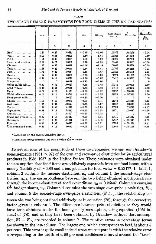
TABLE 1
TWO-STAGE DEMAND PARAMETERS FOR FOOD ITEMS IN THE UNITED STATES*
'YJr/R ~' w, E..,. (E..,.)mR Corrective factort
•Err-Err•E,..- E..,.
E"XlOO
1 2 3 4 5 6 7 8 ---
BeeL .. .............. 1.81 0.47 .02834 -0.95 -1.05 .09572 .050909 -ll.36 Veal.. .... .... ······· 2.23 0.58 .00422 -1.60 -l.61 .01266 .014208 -0.89 Pork .. , ... 1.23 0.32 .02194 -0.75 -0.82 .06975 .007620 -1.02 Lamb and mutton .... 2.50 0.65 .00180 -2.35 -2.35 .00453 .008282 -0.35 Chicken .... ...... ... 1.42 0.37 .00919 -1.16 -1.19 .03067 .006738 -0.58 Turkey, .... .... .. 1.88 0.49 .00229 -1.40 -1.41 .00765 .004659 -0.33 Fish .......... ....... 1.62 0.42 .00553 -0.65 -0.67 .01882 .006796 -1.05 Butter ......... .. ... 1.27 0.33 .00396 -0.85 -0.86 .01274 .001665 -0.20 Shortening ....... .... 0.46 0.12 .00251 -0.80 -0.80 .00410 -.000767 0.10 Margarine. ...... () 0 .00158 -0.80 -G.80 0 0 0 Other edible oils....... 0.12 0.03 .00320 -0.46 -0.46 .00146 - .000399 0.09 Lard (direct) .. ....... -0.19 -0.05 .00136 -0.40 -0.40 -.00114 .000382 -0.10 Eggs .. ........... ... 0.62 0.16 .01128 -0.30 -0.32 .02322 - .003236 1.08 Fluid milk and cream. 0.62 0.16 .02786 -0.29 -0.35 .07536 -.007993 2.76 Evaporated milk .. 0 0 .00172 -0.30 -0.30 0 0 0 Cheese........ ....... 1. 73 0.45 .00375 -0.70 -0.71 .01274 .005814 -0.83 Ice Cream .. ...... 1.35 0.35 .00590 -0.55 -0.57 .01938 .003410 -0.62 Fruits ...... .. ...... 1.54 0.40 .01839 -0.60 -0.66 .06230 .018743 -3.12 Vegetables ..... ... 0.58 0.15 .02335 -0.30 -0.35 .04571 .009587 -3.20 Cereals............. 0 0 .01819 -0.15 -0.15 0 0 0 Sugar and syrups ..... 0.69 0.18 .01649 -0.30 -0.34 .03711 - .004342 1.45 Beverages ....... ,,,, 0.88 0.23 .01031 -0.36 -0.39 .02747 -.001343 0.37 Potatoes ... ... 0.31 0.08 .00469 -0.20 -0.21 .00538 - .001221 0.61 Dry beans and peas ... 0.46 0.12 .00392 -0.25 -0.26 .00640 - .001198 0.48
•Calculated on the basis of Brandow (1961). v
t Calculated using equation (78) with a value of., = -0.86.
To get an idea of the magnitude of these discrepancies, we can use Brandow's measurements (1961, p. 27) of the own and cross-price elasticities for 24 agricultural products in 1955-1957 in the United States. These estimates were obtained under the assumption that food items are additively separable from nonfood items, with a money flexibility of -0.86 and a budget share for food mR/m = 0.23177. In table 1, column 2 contains the income elasticities, 77,1 and column 1 the second-stage elasticities, '1/r/R, the correspondence between the two being obtained multiplicatively through the income elasticity of food expenditure, '11R 0.25667. Column 3 contains tile budget shares, Wr. Column 4 contains the two-stage own-price elasticities, Err, and column 5 the second-stage own-price elasticities, (Err)mR' the relationship be
tween the two being obtained additively, as in equation (78), through the corrective factor given in column 6. The differences between price elasticities as they would have been obtained under the homogeneity assumption, using equation (105) instead of (78), and as they have been obtained by Brandow without that assumption, E~, - E,,, are recorded in column 7. The relative errors in percentage terms are shown in the last column. The largest one, which corresponds to beef, is about 5 per cent. This error is quite small indeed when we compare it with the relative error corresponding to the width of a 90 per cent confidence interval around the "true"

35 Giannini Foundation Monograph • N1tmber 30 • September, 1972
value of the own-price elasticity for beef. Again, according to Brandow's estimates (1961, p. 29), the relative error resulting from the variance of the estimator of the elasticity for beef is about 54 per cent.
We cad also determine the size of the misallocation of income to budget categories that results from using global price indexes, that is, the consumer behaves as if the group utility functions were linearly homogeneous instead of the existing local indexes. Measurement of this misallocation in budgeting is only possible locally since the expenditure functions are only defined in terms of total differentials under weak or strong separability.
We saw that, with homogeneous subfunctions, group price and quantity indexes can be defined as in (92) and (93). In differential form the price indexes are given in equation (91) and the total differential of the expenditure function in equation (90). Hence, the difference in local budget adjustments between strong and stronghomogeneous separability is:
where the superscript h indicates that homogeneous separability has been used. This difference is a weighted sum of the distance to one of the second-stage expenditure elasticities, 7/r/R·
X. ESTIMATION OF DEMAND PARAMETERS WITH A QUADRATIC UTILITY FUNCTION
We have seen in section VII how the price and income elasticities of demand can be known from estimation of the second-stage demand parameters, (aqr/apr')mR
and aqr/amR. Correspondence between second-stage and two-stage demand parameters was established through the "fundamental equations of budgeting" (75), (76), and (77) under strong separability and (84), (85), and (77) under weak separability. We shall now deal with the problem of estimation of the second-stage parameters.
Two approaches can be followed: one consists of specifying directly the functional form of the second-stage demand equations; the other of postulating a functional form for the group subfunctions in the utility function and of deriving from it the corresponding second-stage demand equations. In both cases the functional forms specified should not imply any type of separability among items in the group, unless, of course, we have a priori information on the existence of separability within the group, because it would unduly restrict the degree of substitutability or complementarity among items. We shall follow the first approach in section XIV where a system of constant elasticity, second-stage demand equations is specified. In this section estimation of second-stage demand equations, deriving from quadratic utility subfunctions, is analyzed.
In section IV we have seen that, where the functional form of the demand function is postulated directly, the choice of which parameters to treat as fixed in estimation turns out to be largely arbitrary. It, thus, seems more logical, as Houthakker

36 Bieri and de J anvry: Empirical Analysis of Demand
(1961) pointed out, to solve the problem of parametrization at the level of the utility function. 19 The problem with this approach is that all the utility functions that have been specified for empirical analysis of demand imply additivity....:..._the Stone-Geary (Stone, 1954; Geary, 1949), the exponential (Tsujimura, 1960), the direct and indirect addilog (Houthakker, 1960a), the pointwise additive quadratic (Tsujimura and Sato, 1964), and the block-additive quadratic (Radhakrishna, 1968). We have seen that, while the specifications may be satisfactory for broad categories of items (provided, of course, that these categories can be characterized by price and quantity indexes, which is doubtful), they are not acceptable for subfunctions in a separable partition.
Consider the quadratic utility function
1u(q) = a'q + 2q1Aq (111)
where a is an n-coordinate vector of parameters, and A is a fixed negative-definite matrix of order n. It does not imply additivity unless A is further constrained. Its existence can be justified by regarding it as a second-order Taylor expansion of a general utility function around some equilibrium vector of quantities.
The first-order conditions for a maximum of utility under the budget constraint p'q = m are the structural equations
(112)[_:, -:J [J -[~J Inverting the left-hand side matrix as in (9), (22), (23), and (24), we get the demand functions
From the fundamental equations (8), we obtain
' (115)
(116)
(117)
Q = A[A-1 _A -1pp'A-1(p'A-1p)-1] _ A-1p(p'A-1p)-1q' (118)
= AA-1 - (A/Am)qmq~ - qmq' (Frisch decomposition (25))
= AB - qmq' (Slutsky decomposition (10)).
19 Arbitrariness as to the functional form chosen remains.
37 Gia'f!ll!ini JJ'ounaati-On Monogravh • Nqimber 30 • Septemb-er, 1972
Since the marginal utilities must be positive, a and A must be such that a+ Aq > 0. Because A is negative definite, this implies that q'a > -q'Aq > 0. And for q'a > 0 for all values of q;?: 0, we need a> 0. Thus, the parameters of the quadratic utility function must satisfy the two restrictions a + Aq > 0 and a > 0.
An interesting property of the quadratic utility function is that it permits an easy determination of the distance to saturation levels of conswnption provided these exist. Saturation is defined here as the quantity vector q* whose consumption yields the absolute maximum level of utility. It is given by the unconstrained maximum of the utility function
q* = -A-1a.
Defining m* = p'q* as the "bliss income" that permits reaching q*, the demand function (113) can be rewritten as
Using equations (114) and (115), the flexibility of money becomes
;;; >..mm/A= - m · m*-m
Hence, - .! can be used as a welfare indicator since it characterizes the relative v w
distance of current income to the saturation expenditure level m*, evaluated at current prices. For each commodity, the relative distance to saturation is given by
aqi m* - m 1 T/i·qi = am qi = v
w
Hence, knowledge of the flexibility of money and of the income elasticities provides a measure of the relative distance to saturation.
A further advantage of the quadratic function is that, once the structural parameters a and A are known, programming methods have been developed for the estimation of Engel curves by Houthakker (1960b) and of demand functions by Wegge (1968).
The demand equations (113) are highly nonlinear in the parameters a and A and, hence, difficult to estimate. We now turn to the problem of their statistical estimation.
We rewrite the reductid form equations (113) and (114) as:20
qi - Bia - b1mi - B1e1 t = 1, ... , T (119)
At Am me - b;a - biet t =I, ... , T t
20 The vector a can be specified to vary with t as, say, a, + Dz, where z, stands for an a0
s-dimensional vector of observable variables. Since this generalization does not affect the estimation procedures, the simpler specification a, = a will be adhered to.
38 Bieri amd de Janvry: Empirical .t!nalys-is of Demand
where the error term vector ee is assumed to have the properties E(e1) = 0 and E(e1el) = 2;, The variance-covariance matrix of the error terms on the demand equations, that is, B12;B1 is, thus, singular and dependent on t.21
In a first-estimation procedure, the expected value of Xe, E(X1) is treated as a parameter; the demand equations in (119) can be transformed to show E(Xe) explicitly using equation (113).
(120)
The first n - 1 equations from the set (120) are now used in the estimation since this will guarantee a nonsingular variance-covariance matrix (Powell, 1969). We now haven - 1 equations and T observations in time. The parameters contained in the matrix A and the vector a vary with i = 1, ... , n - 1, whereas the parameters E(X1) vary with t = 1, ... , T. Thus, the n - 1 equations represent observations for the vector E(X,), t 1, ... , T, and the T points in time represent the observations for estimating A and a. We have no way of normalizing22 the equations to make them amenable to ordinary regression techniques without getting into the situation of having to estimate parameters which vary with i and t, that is, for which there are no degrees of freedom. An orthogonal regression technique (Malinvaud, 1964) is thus used to estimate the parameters of (120). This procedure is based on minimizing the sum of squares of the residuals subject to an admissible normalization rule. The system of n - 1 equations and T observations can be written as a univariate model and standardized (centered around the means with respect to t) to eliminate the vector a' = [a1 ... a,,_1] from the estimating equations.23
The estimates of the elements of A are then obtained as the solution vector to a determinental equation. The estimates for E(Xi), all t, are recovered as linear combinations of the estimates of A. Finally, using the estimates obtained (including the ones for the vector a), the parameters of the deleted equation can also be recovered. The procedure is described in detail in Bieri and de Janvry (1971a).
A second estimation method consists in using mathematical approximations to linearize the demand functions. For this procedure, equations (120) are pre-multiplied by A - 1 to give:
(121)
These equations are now linearized so that ordinary regression techniques become ' applicable.24 The resulting equations are as follows:
t = 1, ... , T (122)
21 This dependence may not be too serious since B, is homogeneous of degree zero in the price vector p,. The variance-covariance matrix is singular in view of equation (18).
22 That is, reducing the coefficients of one set of variables, to be used as "dependent," to unity.
23 The estimates of the parameter vector a are obtained by using the estimates of A and E (X,), all t.
24 The approximations used are given in Bieri and de Janvry (1971a).

39 Giannin·i Foundation Monograph • NU1nber 30 • September, 197/t
where Pt represents a price index linear homogeneous in all prices and (3 and n are a vector and matrix of parameters to be estimated. Price and income slopes can be measured directly in equations (122) by taking the appropriate derivatives. The structural parameters A and a can also be recovered up to a constant, just as in the procedure first described.2°
XI. PARTITIONS OF THE COMMODITY SPACE
We have outlined in the previous sections a method for estimating the parameters of consumer demand. The method derives rigorously from an extension of the neoclassical theory of consumer behavior obtained through the introduction in this model of the assumption of budgeting of consumer expenditures. We turn in the following sections to an empirical application of the method; but before doing this, it is of importance to obtain some empirical support of the assumption of consumer budgeting. Up to this point, we have relied directly on a rationalization of consumer budgeting as a simplifying device in the face of a complex situation of decisionmaking. While this, indeed, seems to be a sensible behavioral specification, empirical confrontation remains desirable.
Budgeting requires the existence of group price indexes, at least in local form. In turn, existence of group price indexes implies separability of the utility function. We can, hence, test directly for separability of particular partitions of the set of commodities. Tests of separability are necessary but not sufficient for budgeting.
Testing Whether a Given Partition Is Strongly Separable
Consider first the case of pointwise strong separability for which the following test was developed by Pearce (1964). Equations (40) and (41) give the Slutsky substitution terms under pointwise separability. The total differential of the demand equations becomes
dq; = bi [!!__ dpi L (Obi qi)dpi - dm] i = 1, ... , n. (123)Pi i
Subtracting equation (123) for two commodities, i and j, results in
dpj)- all i, J = 1, ... , n. (124)Pi
If the income slopes have been estimated from cross-section data and two observations in time are available for the vectors q and p, dq and dp can be approxi
25 With this method, the parameters fl and 11 are related to A as follows: An element-byelement division of fi/P, and np,/P, gives estimates Ii, say. Using the average 'E, we have
E (X,) A-I [m' t} p,][~J and
(Bieri and de Janvry, 197la).
40 Bieri and de Janvry: Empirical Analysis of Demand
mated by first differences. Equation (124) provides 1/2 n (n -1) estimates of e. Equation (81) permits an extension of this test to the case of strongly separable partitions. A similar extension obtains in testing for strongly separable partitions with homogeneous subfunctions. Subtracting two equations (94) for commodities Rand K gives
(125)
Equations (125) and (124) are the same, except that we are now dealing with quantity and price indexes for aggregate commodities.
At the same time, in providing tests of separability, equations (124), (93), and (125) permit estimation of 0. A treatment of the statistical problems encountered in using these equations to test for equality of the estimated O's is given in Bieri (1969).
Discovering a Partition and the Nature of Its Separability
Separability implies a restriction on the Slutsky substitution terms. Estimation of those without the separability assumption and inspection of the type of restriction they satisfy would, hence, permit discovering whether a set of commodities is partitionable and, also, through what type of separability.
We can always define a parameter of proportionality, ()ih such that
is identically satisfied. Using the Slutsky decomposition (14), this parameter is related to the price and income elasticities through
()ij Wj'YJi'Y/j 11 . . 1a i, J = , ... , n. (126)m E ii + Wj7];
Under strong separability, O;;/m = 0/m for all id, jd ;;"' I. Under weak separability, O;;/m = Ou/m for all id, jEJ ;;"'I. Under block-additivity, O;;/m = -c';; for all id, jEJ ;;"'I. And under Gossen additivity, O;;/m = -c';; for all i andj. Hence, knowledge of the price and income elasticities estimated without the assumption of separability permits the estimation of 0,-;fm and the determination of whether there is Sjparability and of what type.26
Unfortunately, there exist few matrices of price elasticities that have been obtained without the hypothesis of separability, precisely for the same reason as that for which separability is being used-because generally there are not enough degrees of freedom to estimate an unrestricted matrix. We are, hence, confronted with a vicious circle where estimates of the price elasticities are necessary to establish empirically the existence and nature of separable partitions of the commodity space; but at the same time, separability is necessary to estimate these elasticities. One notable exception is Brandow's matrix of price elasticities for. 24
26 It is not possible, though, to distinguish between strong and additive partitions from O;;/m unless we know a priori the value of the money flexibility. See section XII for empirical evidence on v
w.

41 Giannini Foundation Monograph • N~imber 80 • September, 1972
food products (Brandow, 1961) which has not been directly estimated as a whole but constructed from a combination of prior and sample information on the elasticities. While the assumption of block-additivity has been used to calculate the own and cross-price elasticities of the "nonfood" category, it has not been employed explicitly in the quantification of the elasticities of food items. Calculation of the 9iifm from these data indicates a weakly separable partition within food items of two main groups: 1) beef, veal, pork, lamb and mutton, chickens, turkeys, and fish and 2) cheese, ice cream, fruits, sugar, and syrups. It does not seem possible to categorize other food items into groupings. Detailed results are given in de Janvry (1966).
Since few prior estimates of matrices of price elasticities are available and since direct estimation of those from time series data without the assumption of separability is generally impossible, it is important to seek methods that could yield information on the 9;/s from cross-section data. Analysis of the residuals from fits of Engel functions deriving from a quadratic utility function permits this. Correspondence between the variance-covariance matrix of these residuals and the matrix of Slutsky substitution terms was first established by Theil and Neudecker (1958) and later elaborated on by Kuznets (1963, 1965) and Bieri and de Janvry (197la).
With fixed prices, the demand functions derived from the quadratic utility function (see, for example, (113)) can be expressed as
qh = -(Ba),. - bmh - Beh h = 1, ... , H (127)
where we have assumed that the parameter vector a varies over consumers, whereas the parameter matrix A is fixed. 27 The error term Bei. is assumed to have zero expectation and a variance-convariance matrix~" which is singular in view of the budget constraint.
A reduced, linearly independent set of Engel functions for the commodities i = 1, ... , n - 1 can be derived by maximizing a constrained utility function which yields the following equation:28
where the subscripts I and II indicate vectors with the last element deleted and matrices with the last row and column exluded, respectively; p/stands for prfp,., that is, the vector of deflated prices (the last price serves as numeraire).29 The variance-covariance matrix of the error terms now becomes Bn'l:tu,.Bu and is non
singular. For this variance-covariance matrix to be proportional to Bu, we need to have '2u" = ohB1[~ It is shown in Bieri and de Janvry (197la) that this condition
27 In the expression (Ba )h, only the vector a is assumed to vary with h according to ah + Dgh, with gh being an s-dimensional vector of observable variables that take intoa0
account characteristics specific to the individual consumer h. Thus, the Engel functions are linear only after these specific effects have been eliminated.
28 That is, the budget constraint is imposed on the utility function prior to maximization by reducing the quantity vector from n ton - 1 elements.
29 Note that both a,.h and p.. are scalars referring to the last commodity qn.

42 Bieri and de J anvry: Empirical Analysis of Demand
is met if the errors eh are introduced into the first-order maximizing conditions and the consumer is assumed to behave rationally in the sense of minimizing the loss in utility he incurs because of the errors.30This behavioral assumption thus allows us to conclude that the variance-covariance matrix of the errors in the Engel functions is proportional to the Slutsky substitution matrix. This knowledge, together with estimates of the income slopes, thus permits us to detect additively separable partitions of the commodity space.
Cluster Analysis of Demand
Since discovery of partitions via the price elasticities is a difficult task, it is tempting to look directly for groupings of commodities from the cross-sectional correlations among quantities demanded of the various items.31 If decision-making on quantities demanded is done through preliminary budgeting over groups, items within a same budget category will tend to show high intercorrelations among themselves and also similar profiles of correlations with items outside the group. Factor and cluster analyses can then be used to determine these groups.
Tryon's technique of cluster analysis (1964) was used on household budget data collected in 1927-28 in Germany. Nineteen food items and 10 nonfood items were clustered, and the analysis was repeated for each of three types of families: 1) without children, 2) with one child under 16, and 3) with two children under 16. Clusters were determined by first introducing orthogonal axes by principal components in the correlation configurations and then rotated obliquely. Rotated axes are set through the center of gravity (centroid) of the clusters identified, and the definition of the clusters is revised stepwisely until all variables have their highest projection (loading) on the axis of the cluster which they help define. 32
Nearly identical clusters were obtained for each of the three family types. They are:
1. Butter and fats. 2. Milk and eggs. 3. White and rye bread. 4. Meats, fish, cheese, pastry, and coffee. 5. Flour, starch, cereals, and sugar. 6. Beans and potatoes. 7. Vegetables and fruits.
' 8. Rent, furniture, heating, hygiene, and education. 9. Entertainment, vacation, and transportation.
10. Clothing and maintenance of clothing.
The results indicate a separation of food and nonfood items, and the groupings
30 We assume, of course, that the consumer cannot avoid mistakes altogether. 31 Two more methods to determine partitions have been proposed by Bieri (1969): One is
based on revealed preferences; the other makes use of canonical correlation analysis to estimate the parameters of a quadratic utility function from the first-order conditions under the form
l/p; [a; + r a;k qk J= 1/p; [a; + r a;k qk J for all pairs i, j.
32 Further details and empirical results are given in de Janvry (1966).

43 Giannini Foundation Monograph • Number 30 • September, 1972
obtained seem to have a plausible interpretation in terms of budgeting categories. Nevertheless, ease of empirical analysis in the search of separable partitions has been obtained at the cost of difficulty in interpretation of the groupings observed in terms of structure of the utility function.
XII. ESTIMATION OF THE FLEXIBILITY OF MONEY AND INTERNATIONAL COMPARISONS
The flexibility of money appears as a key variable in the estimation of demand parameters with consumer budgeting and block-additive partitions of the utility function since it enters into the specification of the two-stage price elasticities (78) and (79). Frisch (1959) has, in addition, given it a role of its own as a cardinal welfare indicator since it is a transformation of the marginal utility of income. As we saw in section II, ~ is negative if H is negative-definite. It is a function of prices and income and, according to Frisch, it increases from large negative values to small negative values as the level of real income increases. We are interested in getting an empirical estimate of this relationship so that production of ~ may be obtained for specific levels of prices and income and used in the estimation of two-stage price and income slopes. To do this, we collected from the literature all the estimates of ~we could find, together with the levels of income and prices at which they have been obtained.
The flexibility of money has been estimated in a number of studies where use was made of the additivity hypothesis following one or the other of the approaches described in section III. Table 2 gives the values obtained for Xi by Brandow (1961), Powell (1965, 1966), Dillon and Powell (1965), Amundsen (1964), Frisch (1959), Johansen (1964), Barten (1964, 1967, 1968), Theil (1965), Pearce (1961), and Gruen et al. (1967). Table 2 also indicates the country for which~ was obtained, the time period over which it was estimated, the average level of per capita disposable income in U.S. dollars for that period and approximately the year to which it corresponds, and the level of the cost-of-living index in the United States that same year.
If we assume food to be additively separable from all other items in the consumer's budget, other measurements of ~ can be derived from studies where the price and income elasticities of food have been estimated. Using the Slutsky decomposition and the expression ( 41) for the own-price substitution effect under additivity, one gets for the money flexibility
V 17;(1 - W,"TJ;)w= . (129)E;; + W;17;
Evaluating the budget shares in the year corresponding to the average level of disposable income in the sampling interval, we give in table 2 a series of other
v ~ measurements of w based on the econometric analyses of Waugh (1964), Brandow (1961), Burk (1961), Tweeten (1967), Girshick and Haavelmo (1947), Tobin (1950),

----------------
44 Bieri and de Janvry: Empirical Analysis of Demand
TABLE 2
ESTIMATIONS OF THE FLEXIBILITY OF MONEY
v•Country and PeriodAuthor -wcase number
United States 1926-1941Waugh 1.57
2 1
1926-1941Waugh 1.30 3 1948-1962Waugh 1.12 4 1948-1962Waugh .61 5 1923-1941Brandow 1.01 6 1948-1956Brandow .99 7 1955-1957Brandow .86 8 1924-1941Burk 1.96 9 1948-1957Burk .89
10 1922-1941Tweeten 1.53 11 1946-1965Tweeten 1.23 12 1922-1941Girshick and Haavelmo 1.26 13 1929-1941 2.44 14
Tobin 1929-1942 1947-1949
Cochrane and Lampe 1.34
15 1929-1941 1.22 16
Chetty 1922-1941 1.26
17 Fox
1947-1960 1.47Suits and Sparks
Argentina 1950-1963de Janvry 2.97
19 18
Barreiros, Fucaraccio, 1950-1963 3.90and Herschel
Chile 1952-1963 1.1220 Dillon and Powell
Canada 1952-1963 1.5521 Powell
Norway 1.930-195922 Amundsen 3.00
23 2.00 24
Frisch 1959 1950 2.00Johansen
The Netherlands 1923-1939 1950-1961
25 Barten 2.00
26 1921-1939 1948-1958
Barten 2.16
27 1921-1939 1948-1958
Barten 3.14
28 1921-1939 1948-1963
Theil 2.50
United Kingdom 1952-1958 2.0029 Pearce' Australia 1950-1962 2.87
31 30 Gruen et al.
1950-1960 2.35Powell
fit
570 570
1,668 1,668
559 1,520 1, 736
564 1,548
553 1,668
553 566
704 566 553
1,600
380
380
348
1,325
755 863 647
529
476
476
573
778
997 958
Year of -m
1932 1932 1955 1955 1932 1951 1956 1932 1952 1932 1955 1932 1932
1941 1932 1932 1955
1959
1959
1959
1956
1956 1959 1950
1956
1955
1955
1958
1955
1958 1956
pt
47 .6 47.6 93.3 93.3 47 .6 90.5 94.7 47.6 92.5 47 .6 93.3 47 .6 47.6
51.3 47.6 47.6 93.3
101.5
101.5
101.5
94. 7
94.7 101.5 83.8
94. 7
93.3
93.3
100.7
93.3
100.7 94. 7
Predicted v§
-w
1.46 1.46 1.44 1.44 1.47 1.19 1.13 1.47 1.19 1.48 1.14 1.48 1.46
1.34 1.46 1.48 1.17
2.93
2.93
3.09
1.33
1.86 1. 79 1.90
2.31
2.44
2.44
2.28
1.81
1.63 1.61
• -w is Frisch's (1959) money flexibility. t mis the average per capita disposable income in United States dollars. tP is the U.S. Department of Labor's Consumer Price Index for all items (1957-1959 = 100), reproduced in U.S.
Department of Agriculture (1967). v
§Predicted -w is from equation (130). SouncEs: Waugh (1964); Brandow (1961); Burk (1961); Tweeten (1967); Girshick and Haavelmo (1947); Tobin (1950);
Cochrane and Lampe (1953); Chetty (1968); Fox (1954); Suits and Sparks (1965); de Janvry (1970); Barreiros, Fucaraccio, and Herschel (1965); Dillon and Powell (1965); Powell (1965); Amundsen (1964); Frisch (1959); Johansen (1964); Barten 1968, 1964, 1967); Theil (1965); Pearce (1961); Gruen et al. (1967); and Powell (1966).
v

45 Giannini Foundation Monograph • N1tmber 30 • September, 1972
Cochrane and Lampe (1953), Chetty (1968), Fox (1954), Suits and Sparks (1965), de Janvry (1970), and Barreiros, Fucaraccio, and Herschel (1965).
A certain number of studies, where either J;" or Eii and 7/i for food had been measured, were not used because consumption expenditure instead of disposable income had been employed as a budget constraint.33 Assuming savings to be separable from consumption, the relationship between ~ obtained from disposable income and ~ obtained from consumption can be established. The formula is rather complex, and the studies using consumption expenditures were consequently left aside.
We can establish an empirical relationship between~ and the levels of disposable income and prices reported in table 2. This relationship should be homogeneous of degree zero in income and prices.
We fitted the constant elasticity equation
v 1.872 .602 m 2
log. ( -w) = (6.574) (-4. ) log. p R = .46, F 24.61, lei = .24, (130)961
and the linear equation
(131)
Data between parentheses are t-ratios and le[ is the average absolute deviation of the residuals. In all fits the regression coefficients on the real income variable are highly significant.
Table 2 gives the predicted values of _J;" from equation (130), and figure 1 gives a geometrical representation of the observations and the two fits in the space (-~, m/P). Note that, by using for P the cost of living index in the United States, we do not account for intercountry differences in purchasing power of the dollar.34
For Argentina, predicted values of the flexibility of money for 1959 are -2.93 in equation (130) and -2.69 in (131) which are close to the direct estimate -2.97 obtained in de Janvry (1970) for the same year. The two-stage price elasticities, calculated for Argentina in section XIV, are for the period 1960-1963. The average level of per capita disposable income during this period is iii= U.S. $493 and P = 104.9. Both equations (130) and (131) yield for this period a predicted flexibility of money of- - 2.56.
In calculating the two-stage price elasticities (78) and (79), we thus recognize, as Frisch suggested, that J;" is not a fixed parameter but a function of prices and income. We predict ~for a specific year or time span and calculate the price elasticities for this particular point or interval in time.
We saw in section X that, when a quadratic utility function is postulated, knowL
33 As, for example, Goldberger (1967a). 34 If the purchasing power of the dollar is higher in lower income countries, the estimated
equations may underprediet - ! for those countries.

46 Bieri and de J anvry: Empirical Analysis of Demancl
v -w
3.8
3.6
3.4
3.2
3.0
2.8
2.6
2.4
2.2
2.0.
1.8
1.6
1.4
1.2
1.0
.8
.6
.4
.2
80• • 19
•20
• 27
• 30
• 13
·8
.17
12 ~
16" '15 • II • 3
•3
•4
3 4 5 6 7 8 9 10 11 12 13 14 15 16 17 18 19 m p
Fig. 1. International comparisons of the flexibility of money. , edge of ~ permits us to quantify the relative distance to saturation, both for total expenditure from (m* - m)/m -1/~ and for expenditure on each item from (q~ qi)/qi = -r!if~. These are worthwhile welfare indicators to be known since they describe the magnitude of unfilled wants relative to current consumption levels.
From the income elasticities of major categories of items estimated for Argentina in 1963 and given in section XIII, we can calculate the following values;

47 Giannim,.~ Foundation Monograph • Nitmber 30 • September, 1972
Relative distance to saturation levels
in per cent 100 (m* - m)/m 39.1 100 (qf - q.;)/qi
Food 19.3 Cleaning 18.6 Health services 22.8 Housing services 27.2 Clothing 37.3 Recreation 44.9 Personal services 45.3 Education 64.5 Durables 70.0 Vacation 77.6 Servants 88.3 Automotive expenditure 127.5 Real property 130.6 Other expenditures 27.1
These results indicate, for example, that, while unsatisfied wants of food amount to only 19 per cent of current consumption levels, for automotive expenditure and real property they are as high as 128 per cent and 131 per cent, respectively.
XIII. ESTIMATION OF EXPENDITURE FUNCTIONS FOR MAJOR CATEGORIES OF ITEMS
Frisch's scheme (1959) for estimating all price and income elasticities for the quantities demanded of major categories of items, based on the assumption of pointwise additivity, has been used frequently in the literature. The method is appropriate if there exist group quantity indexes. As we saw in section VIII, this is the case only if Hicks' theorem on composite goods is satisfied within each separable group or if the separable subfunctions in the utility function are homogeneous of degree one. Direct observations of price variations show that the first case is not encountered in practice. Available estimates of the elasticities of quantities demanded of individual items in a same group-food, for example-with respect to group expenditure are generally not all equal to one, contradicting the second case.
Since group quantity indexes are unlikely to exist, it seems reasonable to shift the emphasis from quantities demanded of major categories of items to group expenditure levels and to look for a way of determining the changes in group expenditure levels resulting from changes in the prices of specific items and of income. The first-stage expenditure functions (66) and the price indexes (65) enable us to predict these changes, based on the assumption of strong separability.
We have seen in section VIII that the total differential of the expenditure function, where either Hicks' theorem is satisfied or the utility subfunctions are homogeneous, is:
48 Bieri and de J anvrfl: Empirical Analysis of Demand
Under Hicks' theorem, dPR/PR = dpRI/PRI, and with homogeneous subfunctions, dPR/PR = I: q,.d,p,/mR. By analogy to (132), we can rewrite the expenditure
r
function (66) as:
dmR = (1 + bR)(ObR + mR)dPR bR I: (8bK +mK)dPK bRdm + mR.dz (133) K,,.<R
by defining the group price indexes as:
(134)
h * - 8prb, + p,q, . w ere a, - 8bR + mR
In (133) the first-stage price slopes are, with block-additivity,
(135)
(136)
All the elements that enter into these slopes are observed or estimable from crosssection data. This is also true for the a~'s which can be rewritten as:
(137)
The advantage of rewriting the expenditure function (66), as in (133), is that the sl?pes (135) and (136) can now be used to characterize the change in group expenditure that would result from imposing an equal rate of change in all the prices of a group or to trace the impact on group expenditure of a rate of change dp,/p, in the price of one particular item. In this case the first-stage slopes (135) and (136) must be multiplied by a: of equation (137). We now turn to an empirical example, using Argentine data.
Using a consumer budget survey made in 1963 in all major cities of Argentina, income elasticities are estimated from constant elasticity Engel functions relating expenditure on individual items to total expenditure. These elasticities are reported in table 3 together with the budget shares w, and WR. The elasticities for the budget categories, 11R, are calculated as I:w,71,/wR. The weights a: of the local group
r
price indexes (134) are then calculated according to equation (137).

49 Giannini Foundation Monograph • Number 30 • September, 1972
TABLE 3 WEIGHTS OF GROUP PRICE INDEXES
'11R,1)rt
Food.......·...... ., ....... .. , ......... Meat and fish .. .... ...... ,,, ........ Potatoes ........ ,, .................... Fruita and vegetables ................. Bread and starches................ , , .. Milk and cream .. .................... Sugar ................... , ............. Oil.. ...................... ........... Cheese ... , ... , .... , ··················· Nonalcoholic drinks .................... Beer ...... ························· Wine......... , ... . ' .. . . Other alcoholic drinks.................. Other foods ......................
Cleaning .. , ...................... , .. Health services ................... Housing services ..... , ................... Clothing.................. , .............. Reereation ..... , ............ , ............ Personal services ......................... Education ............................... Durables.... , ... , .... ·················· Vacation ................................. Servants ......... ............ ,, Automotive expenditure ......... ,, ...... Real property........ , . , ················ Other expenditures...... ················
0.494 0.504 0.337 0.560 0.304 0.577 0.318 0.321 0.679 0.618 I. 766 0.380 1.407 0.505 0.475 0.584 0.696 0.956 1.149 1.160 1.651 1.791 1.987 2.261 3.265 3.344 0.694
WR,Wr
0.403 0.108 0.022 0.068 0.034 0.026 0.015 0.014 0.012 0.020 0.002 0.020 0.002 0.060 0.024 0.049 0.088 0.102 0.067 0.043 0.016 0.048 0.022 0.017 0.063 0.010 0.036
a,.t
0.2667 0.0587 0.1633 0.0921 0.0699 0.0404 0.0376 0.0271 0.0467 0.0019 0.0524 0.0028 0.1481
t All the estimated elasticities are significant at the 95 percent confidence level.
The observed expenditure levels mR of budget categories are given in the last column of table 4. From those and the information contained in table 3, the firststage price slopes are computed using equations (135) and (136) and reported in the body of table 4.
The results indicate, for example, that a 10 per cent increase in all food prices leads to an increase of 1,358 pesos (1963) in food expenditure, to a decline of 72 pesos in automotive expenditure (due to the high income elasticity of this budget category), and so forth. On the other hand, an increase of 10 per cent in the price of
meats and fish alone results in a change in the price index for food of a: dp,Pr
(.2667)(.1) = .0267. Since amR/aPR for food is equal to 13,579 pesos, this change induces an increase in food expenditure of (.0267)(13,579) = 362 pesos which represents an increase of 1.7 per cent over the observed level.
XIV. ESTIMATION OF SECOND-STAGE AND TWO-STAGE DEMAND PARAMETERS
With the money flexibility predicted in section XII and the income elasticities estimated in section XIII, we now measure the second-stage elasticities (Err')mR
and '1/r/R in order to know the two-stage elasticities of demand (78), (79), and (80). Continuing with the example on Argentine data, we make use for this purpose of

TABLE 4
FIRST-STAGE PRICE SLOPES (amn/aPx)
Food Cleaning
Health services
Hou:;ingservices
Clothing
Recreation
Personal services
Education
Durable3
Vacation
Servants
Automotive expenditure
Real property
Other expenditures
mB*
Food................ ..........
1988 pesos
13,579 -203 -393 -665 -664 -~ -244 -59 -150 -51 -21 180 51 -272 21, 011 Cleaning ...... ...... ...... ... -193 l,088 -22 -38 -38 -22 -14 -3 -9 -3 -1 10 3 -16 1,251 Health services ....... ..... -485 -29 l,916 -96 -95 -55 -35 -8 -22 -7 -3 26 7 -39 2,555 Housing services .... ,, .. ,,, ... -1,038 -62 -121 3, 136 -204 -118 -75 -18 -46 -16 -6 55 16 -84 4,588 Clothing ...... ..... , .. , ....... -1,653 -99 -192 -326 3,007 -188 -120 -29 -73 -25 -10 88 25 -133 5,318 Recreation . .. ············ ..... -1,306 -78 -152 -257 -257 1, 777 -94 -23 -58 -20 -8 70 20 -105 3,493 Personal services . ..... , .. ... ... -848 -51 -99 -167 -167 -96 1, 165 -15 -38 -13 -5 45 13 -68 2,242 Education....... ............ .. -448 -27 -52 -88 -88 -51 -32 288 -20 -7 -3 24 7 -36 834 Durables.................. .... -1,458 -88 -170 -287 -287 -166 -105 -25 687 -22 -9 78 22 -118 2,503 Vacation ..... , ........... ..... -741 -45 -86 -146 -146 -84 -54 -13 33 246 -5 40 11 -60 1, 147 Servants .... ........... .. ..... -651 -39 -76 -128 -128 -74 -47 -11 -29 -10 100 35 14 -53 887 Automotive expenditure ...... , -3,488 -210 -406 -687 -685 -396 -252 -61 -155 -53 -21 -718 53 -281 3,285 Real property.............. .... -907 -55 -106 -179 -179 -103 -66 -16 -40 -14 -6 48 -244 -73 834 Other expenditures......... -424 -25 -49 -84 -84 -48 -31 -7 -19 -6 -3 23 6 1,334 1,877
*Per capita mR was obtained from CONADE (1967) using an average family size of 3.9 according to CELADE (1967).

51 Giannini Foundation Monograph • Number 30 • September, 1972
time series on consumption of 23 food products elaborated by Nunez (1971) for the period 1938-1967. The data, which are the only ones presently available on consumption, are constructed from production, import, export, intermediate demand, and stock variation data. They therefore characterize consumer demand at the wholesale level, measured in raw-product units-for example, in wheat instead of bread.
The functional form specified for the second-stage demand equations should not imply any kind of separability among items in a same group. For this reason and because of their empirical merits, constant elasticity equations are used. Food expenditure and individual commodity quantity data are on a per capita basis. To take into account the effect of aggregation over individuals, two additional variables have been introduced into the demand functions: One considers the distribution of income which is characterized by the share of wages, z1, in the net national income, z2; the other, the degree of urbanization measured by the proportion of rural, Z4, to total population, za.
Furthermore, the prevalence of habits in consumption is taken into account through the specification of a Nerlovian partial adjustment scheme which results in the introduction of the one-year lagged quantity variable in the demand functions. Alternative regressions are run with and without the z and lagged quantity variables; and from these, the best in terms of goodness of fit as judged by the adjusted R2 were retained.
The budgeting procedure has permitted reducing the number of prices entering the demand functions from a total of n to np35 ; this number, however, is still large so that a further reduction is required in order to avoid the problem of multicollinearity and an excessive loss of degrees of freedom. A workable procedure consists of using a statistical approximation by pooling into a principal components index the prices of all items which are not closely related to the quantity of the commodity in a particular demand function. This index, which thus varies from equation to equation, is then used as a numeraire.
The ordinary least-squares estimates of the second-stage demand functions are presented in table 5.
Since expenditure shares for individual items are based on food expenditure at the wholesale level, that is, WrfF = Prqr/mF, these are transformed into budget shares, using the National Account Statistics (United Nations), in which the average share of raw food in total consumption expenditures is given as Wp = mp/m = .15 for the years 1960-1963. To calculate the two-stage price and income elasticities,
we also need 7/F = aamF . ~which, from the National Account data, is estimated m mp
to equal 0.48 with a variance of 0.04 (Sjastaad, 1966). On the basis of these two pieces of information and of the estimated second-stage
demand functions, we can then calculate the two-stage elasticities which are presented in table 6.36 All other goods (group NF) are assumed separable from food.
36 The subscript F, instead of R, now denotes the budget category Food. 36 All the second-stage elasticities are long run: for the equation estimated without the
lagged quantity variable, the price and income coefficients represent directly the long-run elasticities; for those estimated with the habit-formation variable, the elasticities are computed, following Nerlove's partial adjustment model, by dividing the price and income coefficients by one minus the coefficient of the lagged variable.

TABLE 5
ESTIMATES OF SECOND-STAGE DEMAND FUNCTIONS
Constant (Err)mF f/l'/F
.:!. ~ q-1t R' D.W.term .. •• Beef Lamb Pork Fish
Beef. .... , .. , 2.690 -0.401 0.062 0.082 -0.073 0.236 0.478 0.157 0.132 0.00 1.64 (2.41) (-5.33) (0.89) (1.10) (-1.95) (1.62) (2.60) (0.68) (1.08)
Lamb..... ... , .. 0.340 0.050 -0.244 0.002 0.134 -0.039 -0.291 -1.253 0.87 1. 79 (0.30) (0.48) (-2.47) (0.02) (2.36) (-0.19) (-1.16) (-3.61)
Pork ...... ..... -1.512 0.235 0.168 -0.835 0.034 0.499 0.545 0.87 2.18 (-1.10) (1.64) (1.32) (-5.75) (0.52) (1.77) (6.08)
Fish .. ....... .. 5.241 0.520 -0.085 -0.024 -0.388 -0.299 0.464 1.086 0.82 1.00 (1.99) (2.57) (-0.48) (-0.13) (-4.76) (-0.84) (1.95) (2.01)
Milk
Milk ............. 2.619 -0.335 0.353 0.271 -0.435 0.57 1.66 (3.72) (-3.55) (2.72) (1.76) (-2.75)
Wheat Rice
Wheat............ 1.982 -0.032 0.031 0.175 0.464 0.31 2.29 (1.72) (-0.35) (0.56) (1.14) (2.52)
Rice............. -5.078 -0.521 -0.422 1.021 -0.036 0.007 0.085 0.39 1.14 (-1.86) (-1.78) (-1.60) (2.03) (-1.04) (0.20) (1.15)
Potatoes
Potatoes ......... 4.070 -0.157 0.092 -0.154 0.34 2.35 (2.69) (-2.67) (0.29) (-0.93)
Garlic Onions Tomatoes
Garlic............ -1.802 -0.204 -0.075 0.076 1.043 -1.064 3.019 0.362 0.85 2.06 (-0.51) (-1.89) (-0.42) (0.50) (1.48) (-1.44) (2.73) (2.68)
Onions ........... -l.183 -0.100 -0.420 0.068 0.911 -1.501 2.468 0.65 2.05 (-0.43) (-1.21) (-2.99) (0.57) .. (1.71) (-2.62) (4.02)
Tomatoes ........ -1.976 -0.119 -0.342 -0.132 1.391 0.409 1.708 0.79 2.16 (-0.85) (-1.71) (-2.89) (-1.31) (3.11) (0.85) (3.31)

TABLE 5-Continued
Constant term (E,,)mF 'lr/F !.':.
Z2 !.':.
"" q_1t JJ:l D.W.
Grapes...........
Tangerines......
Apples.........•.
Oranges..........
Pears ............
Peaches ..........
Peanuts..... , ....
Sunflower... , ...
Cottonseed... ...
Sugar............
Mate.............
2.456 (1.49)
-3.273 (-2.16) -0.222
(-0.11) -2.207
(-1.53) -3.582
(-L20) -6.876
(-3.12)
-1.447 (-0.36)
2.068 (0.73)
-2.741 (-0.66)
5.900 (3.59)
-0.702
Grapes
0. 742 (2.15)
0.941 (2.87) 0.632
(1.42) 0.794
(2 .47) 0.989
(1.64) I. 717
(3.62)
0.251 (0.28) 0.142
(0.21) 0.460
(0.47)
-0.161 (-0.80)
0.113
-0.894 (-2.68)
0.077 (3 .42)
-0.023 (-0.74)
0.102 (1.34)
0.244
2.133 (6.42)
0.000 (0.02)
-0.018 (-0.65)
0.056 (0.81)
-0.659
0.267 (1.92) 0.453
(2.30)
0.347 (l.43) 0.503
(2.83) 0.378
(1.94)
0.404 (2.97)
0. 752
0.67
0.85
0.84
0.83
0.76
0.71
0.56
0.40
0.27
0.69
0.75
1.97
2.12
1.98
1.88
2.34
2.14
I. 78
1.85
2.28
2.14
2.65
-0.311 (-3.20)
Tangerines Apples Oranges Pears Peaches
-0.885 (-8,85) -0.120
(-0.88) 0.187
(l.50) 0.009
(0.05) -0.045
(-0.31)
0.638 (8.87)
-0.445 (-4.54)
0.226 (2.49) 0.186
(1.47) 0.201
(1.94)
0.375 (3.73) 0.445
(3.25) -0.753
(-7.53) 0.158
(0.79) 0.087
(0.60)
-0.739 (-5.00) -0.175
(-0.87) -0.147
(-0.84) -0.817
(-3.19) -0.386
(l.78)
0.181 (1.59) 0.112
(0. 72) 0.038
(0.35) 0.328
(I. 70) -0.763
(-4.64)
Peanuts Sunflower Cottonseed
-1.932 (-1.60)
0.583 (1.10)
-0.694 (-0.91)
1.612 (1.43)
-0.062 (-0.13)
0.350 (0.48)
-0.432 (-0,73) -0.096
(-0.25) -0.439
(-0.71)
Sugar
0.314 (3 .75)
Mate Coffee
-0.084 0.041 (-0,68) (-0.78) (0.67) (0.59) (0.90) (-1.89) (3 '78)
Coffee... , .. ,, .... -5.180 -0.107 -0,337 1.140 0.358 -1.010 -0.366 0.47 2. 14 (-2.01) (-0.41) (-2.14) (2.41) (0.63) (-1.42) (-1.48)
t One year lagged quantity.

Bieri and de J an·vry: Empirical Analysis of Demand
TABLE 6
TWO-STAGE PRICE AND INCOME ELASTICITIES
E,,, E,,NF
Beef Lamb Pork Fish
Beef.. ... ., .... ' - .408* .078 .101t -.082* -.064 Lamb... .. ... .042 .245* .001 .134* .009 Pork .. . . . . . . . .- . . .734* .396t -1.809* .083 -.257 Fish ...... ...... .460 - .092* -.031t -.390 .070
Milk
:\[ilk .... ........ - .287* -.083
Wheat Rice
Wheat ... ..... -.029 .060 .076 Rice.... ... - .463* .453* .262
Potatoes
Potatoes ..... .... -.132* -.019
Garlic Onions Tomatoes
Garlic.... - .313* -.107 .158 !
.383 Onions ...... ..... - .096t -.414* .090 .214 Tomatoes. ..... - .113* -.332* - .099f .326
---Grapes
---Grapes. ....... - .257* .174
Tangerines Apples Oranges Pears Peaches
Tangerines .... -.879* .655* .393* -.736* .190t .221 Apples .. ....... -.116 -.434* .457* -.173 .118 -.148 Oranges ... ... .261f .327* -1.006* -.198 .063 -.254 Pears .. .027 .373t .323 -1.489* .618* .424 Peaches .... ..... -.035 .232f .121 -.38lt - .746* .401
Peanuts Sunflower Cottonseed
Peanuts .. -1. 952t 2 .483t - .626 -.090 Sunflower.. 1.178t -.US .192 .067 Cottonseed .. -1.103 .590 .703 .173
---Sugar
---su,,r .... .. , .. .509* .063
Mate Coffee
Mate .. ...... .... -.334 .170 -.107 Coffee .. ..... .. -.068 - .238* -.193
~' w,
Percent
.131t 3.39 -.019 .41
.527t .48 - .144t .12
.169* 2.34
.156 1.64
.536* .14
.038 .92
.784 .09
.437t .14
.668* .51
.356" 1.37
.452t .11
.303t .33
.520" .38
.868t .08
.824* .24
.184 .29
.137 .62
.355 .08
-.130 1.02
.219 .21
.401* .21
• Significant at the 90 percent confidence level. t Significant at the 70 percent confidence Jevol
The budget category NF has an income elasticity of 1.09 from the Engel aggregation equation. We note that, because of the low money flexibility for developing countries such as Argentina, cross-group elasticities tend to be negative, indicating complementarity between budget categories at low income levels.
The significance levels indicated in table 6 pertain to the calculated two-stage

55 Giannini Foun&tion Monograph • N1tmber 30 • September, 1972
parameters. Because the corrective terms relating second-stage to two-stage price elasticities are quite small, the significance levels of the first parameters are taken as a lower bound to the significance levels of the second. Under the assumption that the random terms in the expenditure and demand equations represent errors in the maximization process of the utility function, the residuals will not be correlated when they belong to equations that correspond to different decisions. For this reason, the residuals in the first-stage expenditure functions are not correlated with the residuals in the second-stage demand equations; nor are the residuals in the second-stage equations correlated with each other when they pertain to different budgeting categories. Hence,
Cov (71p, 11r;F) Cov (11r;F, 11k/K) = 0.
Significance levels of the second-stage income elasticities are, hence, calculated from the approximation
Estimates of all cross-price elasticities between food products are not available since, in each second-stage demand equation fitted, a number of prices were collapsed into a principal components index. Further assumptions on the structure of the utility function are necessary to derive them from available parameters. If the restrictive assumption is made that subgroups within food items are block-additively separable, all cross-price elasticities could then be recuperated from equation (79). The assumed partition of food products into separable groups is similar to the one specified in de Janvry and Bieri (1969, p. 38).
ACKNOWLEDGMENT
The authors are deeply indebted to Professor George M. Kuznets for his original contributions to the content of this Monograph and for the excellence of his teaching in demand analysis which aroused our interest to pursue research in this field.
GLOSSARY OF SYMBOLS
n = number of items in the con z = s-coordinate vector of exogesumer's budget no us variables affecting con
q = n-coordinate vector of quanti sumer choices other than curties demanded rent prices and income
p = n-coordinate vector of prices >.=Lagrange multiplier m = disposable income or total ex
Uq = n-coordinate vector of marginal penditure utilities Ui = au/<Jq;u(.) = thrice-differentiable utility
function with positive marginal H = n X n Hessian matrix of eleutility everywhere ments Ui; = a2u/aqia~
a = vector of parameters H CiH>> = i X i principal minor of H
56 Bieri and de Janvry: Empirical Analysi,s of Demand
P<•l = i-coordinate vector composed R, K = subscripts used to index groups, of the i first coordinates of p R,K I, ... ,S.
Q = n X n matrix of Cournot price PR = price index of group R slopes aqi/ap1 QR = quantity index of group R
qm = n-coordinate vector of income fR(.) = separable subfunction of a utility functionslopes aq./8m
hp = n-coordinate vector of elements mR = expenditure on group R ax/ap. WR = budget share of group R, wn =
Am = marginal utility of income mn/m bR = negative of income slope of exax/am
Q. = n X s matrix of elements penditure on group R, bR = -amR/iJmaq./az1
x. = s-coordinate vector of elements '1/R = income elasticity of expenditure on group R, '1/R = -bR/WRiJX/iJz;
a, = price weights in local groupu,. = n X s matrix of elements price index dPR8u./8z1
I,. = n X n identity matrix a~ = weights of rates of change in b -qm prices in local group price index
bo =-Am dPR XB = n X n matrix of Slutsky sub q., = aq,/az
stitution terms Xb.1 mR = amR/az E = n X n matrix of Cournot price brtR = -aq,/amR
elasticitiesEi; = (aq./ap1)(p1/q;) '1/rtR = (aq,/amR)(mR/q,) '1/ = n-coordinate vector of income Wr/R = p,q,/mR
elasticities '1/i = (iJq;fiJm) (m/q;) a = n-coordinate vector of paramew = n-coordinate vector of budget ters in quadratic utility func
shares w, = p;q,/m tion E* = n X n matrix of Slutsky price A = n X n negative-definite matrix
elasticities E~ of parameters in quadratic utility functionE** = n X n matrix of Frisch price
q* = n-coordinate vector of saturaelasticities E~* tion levels D = determinant of the bordered
m* "bliss income" that permitsHessian matrix reaching q*
D;J = cofactor of the (i, j)th element e n-coordinate vector of random J of the bordered Hessian matrix
disturbances with moments (O,D;o = cofactor of the (i, n l)st eleli)ment of the bordered Hessian
fJ variable used in the definition of matrix strong separability in equation D,, diagonal matrix whose elements (36)are the arguments of the vec
fJnK variable used in the definitiontor x of weak separability in equa~ = "flexibility of money" orincome tion (32)
elasticity of X 'lf'R = - L,9RKbK/(l + bR), see equaqo = optimizing value of q K,,sR
v(.) = indirect utility function tion (71).
57 Giannini Foundation Monograp·h • Number 30 • September, 1972
LITERATURE CITED
AMUNDSEN, A. 1964. Private consumption in Norway, in Europe's future consumption (J. Sandee, ed.) Am
sterdam: North-Holland Publishing Company, pp. 162-64. BARREIRos, I. A., A. FucARAccrn, and F. HERSCHEL
1965. Funciones de consumo en la Argentina. Paper presented at the second meeting of the Argentine Economic Association, p. 30.
BARTEN, A. P. 1964. Consumer demand functions under conditions of almost additive preferences, Econo
metrica, 32(1-2) :1-38. 1967. Evidence on the Slutsky conditions for demand equations, Rev. of Econ. and Stat.,
49(1) :77-84. 1968. Estimating demand equations, Econometrica, 36 (2) :213-51.
BARTEN, A. P., and S. J. TuRNOVSKY 1966. Some aspects of the aggregation problem for composite demand equations, Internat.
Econ. Rev., 7(3):231-54. BASMANN, R. L.
1956. A theory of demand with variable consumer preferences, Econometrica, 24(1) :47-58. BIERI, JURG HANS
1969. The quadratic utility function and measurement of demand parameters, unpub. Ph.D. diss., Dept. of Agric. Econ., Univ. of California, Berkeley.
1972. Decentralizability in demand analysis and second-stage demand functions. Giannini Foundation of Agric. Econ., Univ. of California, Berkeley (mimeo.).
BIERI, J., and A. DE JANVRY 1971a. The quadriatic utility function: estimation of demand parameters. Giannini Foundation
of Agric. Econ., Univ. of California, Berkeley. 1971b. Aggregation, budgeting, and separability in demand analysis. Giannini Foundation of
Agric. Econ., Univ. of California, Berkeley (mimeo.). BLACKORBY, C.
1968. Rational rules for intertemporal decision making. Dept. of Econ., Univ. of California, Santa Barbara (mimeo.).
BOUTWELL, wALLACE K., JR., and RICHARD L. SIMMONS 1968. Estimation of demand for food and other products assuming ordinally separable utility,
Amer. Jour. of Agric. Econ., 50(2) :366-78. BRANDOW, G. E.
1961. Interrelations among demands for farm products and implications for control of market supply, Penn. Agric. Exp. Sta. Bui. 680.
BURK, MARGUERITA, C. 1961. Trends and patterns in U.S. food consumption, Econ. Res. Serv., U.S.D.A., Agriculture
Handbook No. 214, Table 3.2. BYRON, R.
1970. A simple method for estimating demand systems under separable utility assumptions, Rev. of Econ. Stud., 37:(110) :261-74.
CELADE 1967. Estimaci6n del mimero de hogares familiares segun sexo-edad del jefe, 1960-1980, Argen
tina, Series C, No. 83. Santiago, Chile. CHETTY, v.
1968. Pooling of time series and cross section data, Econometrica, 36(2) :279-90. CLARKSON' G.
1963. The theory of consumer demand: a critical appraisal. New York: Prentice Hall, Inc. CocHRANE, W., and H. LAMPE
1953. The nature of the race between food supplies and demand in the United States, Jour. of Farm Econ., 35(2) :203-22.
CoNADE 1967. Estudios de politica fiscal en la Argentina, Bui. No. 65, Vol. VI. Buenos Aires, Argentina.
CRAMER, JAN SALMON 1962. The ownership of major consumer durables: a statistical survey of motor cars, refrig
erators, washing machines, and television sets in the Oxford savings survey of 1953. Cambridge: Cambridge Univ. Press.

58 Bieri and de Janvry: Empirical Analysis of Demand
DE JANVRY, ALAIN 1966. Measurement of demand parameters under separability, unpub. Ph.D. diss., Dept. of
Agric. Econ., Univ. of California, Berkeley. 1970. Estimaci6n de sistemas de ecuaciones de gastos y demanda, Economica (La Plata),
16(1) :31-59. DE JANVRY, ALAIN, and JuRG BIERI
1969. On the problem of degrees of freedom in the analysis of consumer behavior, Amer. Journ. of Agric. Econ., 50(5) :172o'.-36.
DILLON, J., and A. POWELL 1965. Un modelo econorpetrico de la demanda al detalle en Santiago de Chile, Cuadernos de
Economia, 2(7) :31'--38. DoBELL, A. R.
1965. A comment on Anthony Y. C. Koo's "An empirical test of revealed preference theory,'' Econometrica, 33(2) :451-55.
Fox, KARL A. 1954. Structural analysis and the measurement of demand for farm products, Rev. of Econ. and
Stat., 36(1) :57-66. FRISCH, RAGNAR
1959. A complete scheme for computing all direct and cross demand elasticities in a model with many sectors, Econometrica, 27(2):177-96.
GEARY, R. 1949-1950. A note on "A constant-utility index of the cost of living," Rev. of Econ. Stud.,
18(45) :65-66. GEORGE, P. S., and G. A. KING
1971. Consumer demand for food commodities in the United States with projections for 1980. Univ. of California, Giannini Foundation Monograph 26. Berkeley.
GrnsmcK, M.A., and TRYGVE HAAVELMO 1947. Statistical analysis of the demand for food: examples of simultaneous estimations of
structural equations, Econometrica, 15(2) :79-110. GOLDBERGER, A.
1967a. A cross-country comparison of consumer expenditure patterns. Univ. of Wisconsin, Systems Formulation, Methodology, and Policy Workshop Paper 6706.
1967b. Functional forms of utility: a review of consumer demand theory. Univ. of Wisconsin, Systems Formulation, Methodology, and Policy Workshop Paper 6703.
1969. Directly additive utility and constant marginal budget shares, Rev. of Econ. Stud., 36(106) :251-54.
GOLDMAN, S. M., and H. UzAwA 1964. A note on separability in demand analysis, Econometrica, 32(3) :387-98.
GORMAN, w. M. 1959. Separable utility and aggregation, Econometrica, 27(3) :469-81.
GREEN, H. A. JOHN 1961. Direct additivity and consumers' behaviour, Oxford Economic Papers, 13(2) :132-36.
GRUEN, F. H., A. A. PowELL, B. W. BROGAN, G. C. McLAREN, R. H. SNAPE, T. WACHTEL, and L. E. WARD
1967. Long term projections of agricultural supply and demand, Australia, 1965-1980. Vol. 1. Clayton, Victoria, Australia: Dept. of Econ., Monash University, p. 4-12.
Hiqrn, J. R. 1!!39. Value' and capital: an inquiry into some fundamental principles of economic theory.
London: Oxford Clarendon Press. HOTELLING, H.
1932. Edgeworth's taxation paradox and the nature of demand and supply functions, Jour. of Polit. Econ., 40(5) :577-616.
HouTHAKKER, H. S. 1960a. Additive preferences, Econometrica, 28(2) :244-57. 1960b. The capacity method of quadratic programming, Econometrica, 28(1):62-87. 1961. The present state of consumption theory, Econometrica, 29( 4) :704-40.
JOHANSEN, LEIF 1964. A multi-sectoral study of economic growth. Amsterdam: North-Holland Publishing
Company. KLEIN, LAWRENCE ROBERT
1950. Economic fluctuations in the United States, 1921-1941. (Cowles Comm. for Research in Economics, Mono. 11.) New York: John Wiley and Sons, Inc.

59 Gianniini Foundation Monograp·h • Number 30 • September, 1972
Koo, ANTHONY Y. C. 1963. An empirical test of revealed preference theory, Econometrica, 31(4) :646-64.
KooPMANS, TJALLING C., PETER A. DIAMOND, and RICHARD E. WILLIAMSON 1964. Stationary utility and time perspective, Econometrica, 32(1-2) :82~100.
KUZNETS, GEORGE M. 1963. Theory and quantitative research, Jour. of Farm Econ., 45(5):1393-1400. 1965. Notes on measurement of demand under separability. Giannini Foundation on Agri
cultural Economics, Univ. of California, Berkeley (mimeo.). LAu, L. J.
1970. Duality and utility structure, unpub. Ph.D. diss., Dept. of Econ., Univ. of California Berkeley.
LEONTIEF1 WASSILY 1947. Introduction to a theory of the internal structure of functional relationships, Econo
metrica, 15(4) :361-73. MAUNVAUD, E.
1964. Methodes statistiques de l'econometrie. Paris: Dunod. MEYER, J., and E. KuH
1957. How extraneous are extraneous estimates? Rev. of Econ. and Stat., 39(4) :380-93. MISHAN, E. J.
1961. Theories of consumer's behaviour: a cynical review, Econornica, 28(109) :1-11. NuNEz, A.
1971. A quantitative macroeconomic study of Argentinian agriculture, forthcoming Ph.D. diss., Dept. of Econ., Univ. of California, Berkeley.
PAPANDREOu, ANDREAS GEORGE 1958. Economics as a science. Chicage: Lippincott Co.
PARKS, RrcHARD W. 1969. Systems of demand equations: an empirical comparison of alternative functional forms,
Econometrica, 37(4) :629-50. PEARCE, I. F.
1961. An exact method of consumer demand analysis, Econometrica, 29(4):499-516. 1964. A contribution to demand analysis. Oxford, England: Oxford Univ. Press.
POWELL, ALAN 1965. Postwar consumption in Canada: a first look at the aggregates, Canadian Jour. of Econ.
and Polit. Science, 31(4) :559-65. 1966. A complete system of consumer demand equations for the Australian economy fitted by
a model of additive preferences, Econometrica, 34(3) :661-75. 1969. Aitken estimators as a tool in allocating predetermined aggregates, Jour. of the Amer.
Stat. Assoc. 64(327) :913-22. RADHAKRISHNA, R.
1968. A method of deriving price and income effects from family budget data, Metroeconomica, 20(1) :26-32.
RoY, R. 1943. De l'utilite: contribution a la theorie des choix. Paris: Hermann et Cie.
SAMUELSON, P. A. 1947. Foundations of economic analysis. Cambridge: Harvard Univ. Press. 1965. Using full duality to show that simultaneously additive direct and indirect utilities im
plies unitary price elasticity of demand, Econometrica, 33(4) :781-796. SANDEE, J. (ed.)
1964. Europe's future consumption. Amsterdam: North-Holland Pub. Co. SJAASTAD, L.
1966. Consumption patterns in Argentina. Dept. of Econ., Univ. of Chicago, Illinois (rnimeo.). SoNo, MASAzo
1961. The effect of price changes on the demand and supply of separable goods, Internat. Econ. Rev., 2(3) :239-71.
STONE, R. 1954. Linear expenditure systems and demand analysis: an application to the British pattern
of demand, Economic J our., 64(255) :511-27. STROTZ, ROBERT H.
1957. The empirical implications of a utility tree, Econometrica, 25(2) :269-80. 1959. The utility tree, a correction and further appraisal, Econometrica, 27(3) :482-88.
SuITs D. and G. SPARKS 1965. Consumption regressions with quarterly data, Brookings quarterly econometric model of
the United States. (J. Duesenberry et al., eds.) Chicago: Rand McNally &Co., Chapter 7.

60 Bieri ana ae J anvry: Empiriaa:t L'J.nalysis of Demand
THEIL, HENRI 1965. The information approach to demand analysis, Econometrica, 33(1) :67-87. 1967a. Economics and information theory. Amsterdam: North-Holland Pub. Co. 1967b. Lectures on econometrics. Center for Mathematical Studies in Business and Economics,
Univ. of Chicago. THEIL, H., and H. NEUDECKER
1958. Substitution, complementarity, and the residual variation around Engel curves, Rev. of. Econ. Stud., 25(67) :114-23.
TOBIN, J. 1950. A statistical demand function for food in the U.S.A., Jour. of the Royal Stat. Soc.,
Series A, 113(II) :113-41. TRYON, R. c.
1964. Theory of the BC TRY system of cluster and factor analysis. Dept. of Psychology, Univ. of California, Berkeley (mimeo.).
TSUJillWRA, K. 1960. Family budget data and market analysis, Bulletin de l'Institut International de Sta
tistique, 38:215-42. TsuJIMURA, K., and T. SATO
1964. Irreversibility of consumer behavior in terms of numerical preference fields, Rev. of Econ. and Stat., 46(3):305-19.
TWEETEN, LUTHER G. 1967. The demand for United States farm output, Food Research Institute Studies in Agri
cultural Economics, Trade, and Development, 7(3):343-69. UNITED NATIONS, DEPAR'l'MENT OF ECONOMIC AND SOCIAL AFFAIRS
Various issues. Yearbook of national accounts statistics. New York. U.S. DEPARTMENT OF AGRICULTURE
1967. Agricultural statistics, 1967. WAUGH, FREDERICK V.
1964. Demand and price analysis. U.S.D.A., Technical Bui. No. 1316, p. 13. ~~L .
1968. The demand curves from a quadratic utility indicator, Rev. of Econ. Stud., 35(102) :· 209-24.
WILKS, s. 1938. Weighting systems for linear functions of correlated variables when there is no dependent
variable, Psychometrika, 3:23-40. WoLD, HERMAN, and LARS JuREEN
1953. Demand analysis: a study in econometrics. New York: John Wiley and Sons, Inc. ZELLNER, ARNOLD
1962. An efficient method of estimating seemingly unrelated regressions and tests for aggregation bias, Jour. of the Amer. Stat. Assoc., 57(298) :.348-67.
L25m-9,'72 (Q3880) WP ~141

GIANNINI FOUNDATION MONOGRAPH SERIES
What it is
The Giannini Foundation Monograph Series is comprised of technical research reports relating to the economics of agriculture. The series, introduced in 1967, is published by the California Agricultural Experiment Station. Similar technical economic research studies formerly were published in Hilgardia.
Each Monograph is a separate report of research undertaken in the California Experiment Station by staff members of the Department of Agricultural Economics and the Giannini Foundation of Agricultural Economics in the University of California. Topics covered range from analyses of farm and processing :firms to broader problems of interregional resource use and public policy.
The Monographs are written in technical terms with professional economists as the intended audience. No attempt is made to reduce the writing to terms understandable to the layman. Each Monograph carries an abstract on the inside front cover.
Monographs are published at irregular intervals as research is completed and reported.
How to obtain copies
In general, copies will be sent free on request to individuals or organizations. The limit to California residents is 20 titles; the limit to nonresidents is 10. There is no distributi-On through agencies or stores.
A list of available Monographs in the series is published annually and may be obtained by writing to Agricultural Publications (address below). The list also explains how some out-of -print issues, including reports that formerly appeared in Hilgardia, may be obtained on microfilm or as record prints. To obtain the Giannini Foundation Monograph Seri.es regularly, certain minimum qualifications must he met:
As a gift. Some libraries, educational institutions, or agricultural experiment stations may receive Monographs as issued where there is a definite need for the material and it will he made available to a con. siderable number of interested economists. Address requests to Agri' cultural Publications. Please give particulars. ·
As an exchange for similar research material. Address requests to Librarian, Giannini Foundation of Agricultural Economics, University of California, Berkeley, California 94720.
With the exception of communications about exchange agreements (see above) , address all correspondence concerning the Giannini Foundation Monograph Seri.es to:
Agricultural Publications University of California Berkeley, California 94720