demand dynamics under consumer regret: an empirical analysis (supply and demand side)

Demand Dynamics Under Consumer Regret: AnEmpirical Analysis

Meisam Hejazi Nia

with Dr. Ozalp Ozer and Dr. Gonca SoysalUniversity of Texas at Dallas

[email protected]

December 17, 2013

Meisam Hejazi Nia (UTD) Demand Dynamics Under Consumer Regret December 17, 2013 1 / 25

Consumers are Regretful

(a) Fashion Goods (b) Sales (c) Product Availability


Consumers Decision

Utility of Purchase

1 Ownership Utility

2 ConsumptionUtility

Disutility of Purchase

1 Price

Behavioral Elements

1 High Price Regret

2 Stock Out Regret


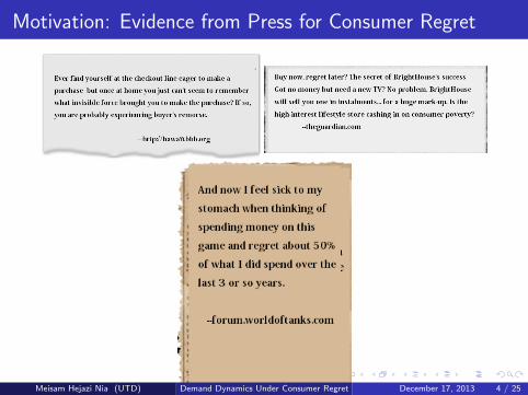
Motivation: Evidence from Press for Consumer Regret


Every day Low price or Promotion Strategy?

Rational Consumer:Forward Looking

Consumer BehaviorFuture Regret

Pricing and MarkdownEmpirical Studies

Soysal & Krishnamurthi (2012)Nair (2007)Li,Grandose & Netessine(2013)

Pricing and MarkdownTheoretical Research

Ozer & Zhang(2013)Nasiry & Popescu (2009)Rotemberg (2010)Decidue, Rudi & Tang(2012)

General(Service, Product as-sortment, product cus-tomization, equity pur-chase, choice model)

Lemon, White & Winder(2002)Gourville & Soman(2005)Solnik (2008)Syam, Krishnamurthi &Hess (2008)Thiene, Boeri & Chorus(2012)


Research Questions

What are the effects of high price regret and stock out regret in purchasedecision of consumers for seasonal goods?

What is the extent of ownership and consumption utility for the fashionproduct?

How much heterogeneity exists in consumers price sensitivity, high priceregret, and stock out regret?

What is firm’s optimal pricing and signaling strategy for seasonal goodswhen consumers are forward looking and regretful?

How optimal strategy and equilibrium result changes when consumers haveheterogeneous price and regret sensitivity, and when consumersexpectations are distorted?


Overview

Data

Leading specialty apparel retailer

Women’s coats: Two years of 105 SKU’s each on average for 30weeks

Weekly sales, revenue, starting inventory, unit acquisition cost

Methodology

Simple regression and Likelihood estimation of aggregate Logit andBLP

General Methods of Moment (GMM)

Delta method


Results

Results

BLP model fits the data better than supply side and withoutheterogeneity models.

Price sensitivity and consumption utility are Significant.

Stock out regret is only significant after accounting for heterogeneity(BLP).

There is second a segment of consumers that are more price sensitive,more regretful to high price, and less regretful for stock out.


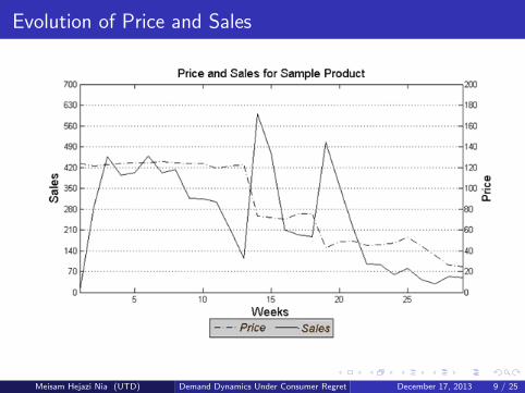
Evolution of Price and Sales


Basic Statistics: Average revenue and quality sold atdifferent relative price points

Relative Price (%) Revenue (%) Quantity sold (%)

70-100 0.896 1.23160-69 0.855 1.32550-59 0.671 1.22440-49 0.966 2.08730-39 1.193 3.19420-29 1.517 6.447< 20 0.081 0.490


Consumer’s Decision

Consumer’sDecision

Purchase

Purchasein firstPeriod

Purchasein second

Period

Not Purchase


First Model:Basic

Model

Ui1 = α + (0.5di1 + ridi2)θ + βppi1

+αpai2(pi1 − pi2) + ξi1 + εi1

i = 1..105, t = 0..2 ,

ri = 11.0025

di1

εit ∼ EV 1(0, π2

6 ) , ξit ∼ N(0, σ2ξ )

Ui2 =

ri (ai2(α + 0.5di2θ + βpPi2)

+(1− ai2)βr (0.5di1 + ridi2)θ) + ξi2 + εi2

Ui0 = εi0

i :Product index

t:Period index (0 for not purchase)

Uit :Utility of Consumer for Purchasein period (t = 0 not purchase)

Pit :Price of product i at period t

ait :Availability of product i at periodt

ri :Discount factor for product i

dit :Duration of period t for product i

ξit:Unobserved aggregate demandshock

α: Ownership utilityθ: Weekly consumption Utilityβp: Price Sensitivityαp: High Price Regret


First Model:Basic

Model



i = 1..105, t = 0..2 ,

ri = 11.0025

di1

εit ∼ EV 1(0, π2

6 ) , ξit ∼ N(0, σ2ξ )

Ui2 = ri (ai2(α + 0.5di2θ + βpPi2)


Ui0 = εi0

i :Product index

t:Period index (0 for not purchase)







α: Ownership utilityθ: Weekly consumption Utilityβp: Price Sensitivityαp: High price regretβr : Stock Out Regret


Second Model:Consumption Heterogeneity

Model

Ui1 = α + (0.5di1 + ridi2)ciθ + βppi1


i = 1..105, t = 0..2 ,

ri = 11.0025

di1

εit ∼ EV 1(0, π2

6 ) , ξit ∼ N(0, σ2ξ )

Ui2 = ri (ai2(α + 0.5di2ciθ + βpPi2)

+(1− ai2)βr (0.5di1 + ridi2)ciθ) + ξi2 + εi2

Ui0 = εi0






ci :Cost of product i (quality)


α: Ownership utilityθ: Weekly consumption Utilityβp: Price Sensitivityαp: High price regretαp: High Price Regret


Third Model:Ownership Heterogeneity

Model

Ui1 = αci + (0.5di1 + ridi2)θ + βppi1


i = 1..105, t = 0..2 ,

ri = 11.0025

di1

εit ∼ EV 1(0, π2

6 ) , ξit ∼ N(0, σ2ξ )

Ui2 = ri (ai2(αci + 0.5di2θ + βpPi2)


Ui0 = εi0








α: Ownership utilityθ: Weekly consumption Utilityβp: Price Sensitivityαp: High price regretβr : Stock Out Regret


Fifth Model:Fixed Effect

Model

Ui1 = αi + (0.5di1 + ridi2)θ + βppi1


i = 1..105, t = 0..2 ,

ri = 11.0025

di1

εit ∼ EV 1(0, π2

6 ) , ξit ∼ N(0, σ2ξ )

Ui2 = ri (ai2(αi + 0.5di2θ + βpPi2)


Ui0 = εi0







αi : Product specific ownership utilityθ: Weekly consumption Utilityβp: Price Sensitivityαp: High price regretβr : Stock Out Regret


Sixth Model: BLP type model

Model

Ui1 = α + (0.5di1 + ridi2)ciθ + βpjpi1

+αpjai2(pi1 − pi2) + ξi1 + εi1

i = 1..105, t = 0..2 , j = 1, 2

ri = 11.0025

di1

εit ∼ EV 1(0, π2

6 ) , ξit ∼ N(0, σ2ξ )

Ui2 = ri (ai2(α + 0.5di2ciθ + βpjPi2)

+(1− ai2)βrj(0.5di1 + ridi2)ciθ) + ξi2 + εi2

Ui0 = εi0








α: Ownership utilityθ: Weekly consumption Utilityβpj : Price Sensitivityαpj : High price regretβrj : Stock Out Regret


Estimation: Aggregate Logit

Basic Model (Demand Side)



εit ∼ EV 1(0, π2

6 ) , ξit ∼ N(0, σ2ξ )

Ui2 =



Ui0 = εi0

Estimation

Ui1 = Vi1 + εi1

Ui2 = Vi2 + εi2

Ui0 = εi0

Sit = eVit∑2s=0 e

Vis

Vi1 = ln(Si1)− ln(Si0)

Vi2 = ln(Si2)− ln(Si0)

Sit = salesitMi

Mi = 1.25Invi


Estimation: BLP

BLP type Model (Demand Side)

Ui1 = α + (0.5di1 + ridi2)ciθ + βpjpi1

+αpjai2(pi1 − pi2) + ξi1 + εi1

εit ∼ EV 1(0, π2

6 ) , ξit ∼ N(0, σ2ξ )

Ui2 = ri (ai2(α + 0.5di2ciθ + βpjPi2)

+(1− ai2)βrj(0.5di1 + ridi2)ciθ) + ξi2 + εi2

Ui0 = εi0L(Ω) =

∏Tt=1 fξ(D

−1t (qt ; Ω)) ‖J‖

‖J‖ =∥∥∥∂D−1

t (qt ;Ω)∂qit

= | ∂ξit∂qit|

= | − ∂G/∂qit∂G/∂ξit

= | − −1∑2k=1 NkitPikt(qt |Ω)[1−pkit(qt |Ω)]

|

Estimation

Ω = (α, c , β, π, σxi )

δi1 = α + c + γc + βp1pi1

αp1ai2(pi1 − pi2) + ξi1

δi2 = ri (ai2(α + c + βp1pi2)

+(1− ai2)βr1((0.5di1 + ridi2)ciθ) + ξi2

β2 = (β2 − β1), , β2 = (β2p, α2p, β2r )

MSi1 = π1iexp(δi1)∑2t=0 exp(δit)

+(1− π1i )exp(δi1+βp2pi1+αp2ai2(pi1−pi2))∑2

t=0 exp(Uit2)

MSi2 = π2iexp(δi1)∑2t=0 exp(δit)

+ (1− π1i )

exp(δi2+ri (ai βp2pi2+(1−ai )βr2ai2(0.5di1+ridi2)ciθ))∑2t=0 exp(Uit2)


Estimation:GMM

Supply Side Model (Model 7)

Ui1 = α + (0.5di1 + ridi2)ciθ + βppi1


i = 1..105, t = 0..2 ,

ri = 11.0025

di1

εit ∼ EV 1(0, π2

6 ) , ξit ∼ N(0, σ2ξ )

Ui2 = ri (ai2(α + 0.5di2ciθ + βpPi2)


Ui0 = εi0

Estimation

π = (pi1 − ci )si1 + ri ((1− di )pi1 − ci )si2∂pi∂pi1

= 0∂pi∂di

= 0

∂pi∂pi1

= ((pi1 − ci )(si1 − s2i1 − si1si2riai (1− di ))

+ri (1− di )(pi1 − ci )[riai si2(1− di )− si1si2

−s2i2riai (1− di )])bp + (pi1di si1 − pi1s

2i1aidi − ri

(1− di )pi1[aidi si1si2])ah + si1 + ri (1− di )si2 = 0

∂pi∂di

= [(pi1 − ci )(riaipi1si2si1) + ri (1− di )

(pi1 − ci )[−riaipi1si2 + s2i2riaiaipi1]]bp

+[pi1(ai si1pj1 − ai si1pi1)− r(1− d)pi1

(si2aipi1si1)]ah − ripi1si2 = 0


Estimation:Delta Method to Identify Stock Out RegretCoefficient

Basic Model



εit ∼ EV 1(0, π2

6 ) , ξit ∼ N(0, σ2ξ )

Ui2 =



Ui0 = εi0

Estimation

η = θβr

V

(θη

)=

(σ11 00 σ22

)

βr = η

θ

µ =

(1θ

− η

θ2

)V (βr ) = µ′V

(θη

)µ


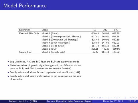
Model Performance

Estimation Model LL AIC BIC

Demand Side Only Model 1 (Basic) -319.46 648.93 662.20Model 2 (Consumption Util. Hetrog.) -317.81 645.61 658.88Model 3 (Ownership Util Heterog.) -318.46 646.92 660.19Model 4 (Both Heterogen.) -318.83 647.66 660.93Model 5 (Fixed Effect) -187.70 593.38 882.66Model 6 (BLP) 206.16 -402.33 -389.06

Supply Side Model 7 (Supply Side) -45.22 104.44 123.02

Log Likelihood, AIC and BIC favor the BLP and supply side model.

Global optimizer of genetic algorithm rgenoud, and DEoptim did notwork on BLP, and GMM (needed for not smooth function).

Supply side model allows for auto regression with coefficient (1.64)

Supply side model uses transformation to put constraint on the signof variables.


Parameter Estimate

Parameter Model1 (Ba-sic)

Model 2(Cons. Hetr.)

Model 3(Ownr. Hetr.)

Model 4 (BothHetr.)

Model 5 (FixedEffect)

Model 6 (BLP) Model 5 (Sup-ply)

Ownership utility(α) 0.34 0.53 0.01 -0.004 0.25 1.10( 0.70 ) ( 0.36 ) ( 0.01 ) ( 0.010 ) ( 0.22 )

Consumption utility(θ) 0.010 0.001* 0.026* 0.001* -0.288* 0.000 0.06( 0.024 ) ( 0.000 ) ( 0.013 ) ( 0.000 ) ( 0.085 ) ( 0.000 )

Price Sensitivity (βp) -0.003 -0.006* -0.006 -0.003 -0.051* -0.003* -8.56( 0.002 ) ( 0.003 ) ( 0.004 ) ( 0.003 ) ( 0.013 ) ( 0.002 )

High price Regret (αp) 0.008 0.008 0.009 0.007 0.166* -0.002 -1.08( 0.009 ) ( 0.009 ) ( 0.009 ) ( 0.009 ) ( 0.039 ) ( 0.005 )

Stock out Regret (βr ) 1.452 0.440 0.009 0.476 0.165 -4.66** 43.88( 2.155 ) ( 0.637 ) ( 0.517 ) ( 0.570 ) ( 0.288 ) ( 1.546 )

Segment Size (π) 0.998

** p < .05, * p < .1.

For supply side model Hessian is negative semi definite, so it is notpossible to calculate standard errors.

For the BLP model second segment heterogeneity parameters were(βp, αp, βr ) = (−3.38e − 9,−0.0005, 0.0140)

Hessian for parameter heterogeneity in BLP is negative.


Finding’s Summary and Conclusion

BLP model fits the data better than supply side and without heterogeneitymodels.

Price Sensitivity and consumption utility are Significant.

Stock out regret is only significant after accounting for heterogeneity(BLP).

There is a second segment of consumers that are more price sensitive,more regretful to high price, and low regretful for stock out.


Thank You


demand dynamics under consumer regret: an empirical analysis (supply and demand side)

Data & Analytics