the demand for education in norway: an empirical analysis
TRANSCRIPT

1
The Demand for Education in Norway: An
Empirical Analysis of Education
Expenditures
Sindre Tytingvåg,
June 2015
UiS Business School
Norsk tittel: Etterspørsel etter Utdanning i Norge,
En Empirisk Analyse av Utdanningsutgifter

2
FACULTY OF SOCIAL SCIENCES,
UIS BUSINESS SCHOOL
MASTER’S THESIS
STUDY PROGRAM:
Master in Business Administration
THESIS IS WRITTEN IN THE FOLLOWING
SPECIALIZATION/SUBJECT:
Economic Analysis
IS THE ASSIGNMENT CONFIDENTIAL? No
TITLE:
The Demand for Education in Norway: An Empirical Analysis of Education Expenditures
NORSK TITTEL:
Etterspørsel etter Utdanning i Norge: En Empirisk Analyse av Utdanningsutgifter
AUTHOR
ADVISOR:
Gorm Kipperberg
Student number:
207410
…………………
Name:
Sindre Tytingvåg
…………………………………….
ACKNOWLEDGE RECEIPT OF 2 BOUND COPIES OF THESIS
Stavanger, ……/…… 2015 Signature administration:……………………………

3
Abstract
The complex development of a country’s economic situation with various components
affecting it in many different ways may lead to important changes as a result of a shift in one
or more important factors. Allocation of scarce resources is crucial for so many different
agents in all sorts of markets. Important decisions will have to be made by an individual, a
firm and a corporation, and this chain of decision making leads all the way up to the central
government of a country. One of these factors that might seem simple at first, but is indeed
very wide is the demand for education in a country. In general, the demand for education
shows not only the quantity of education demanded, but also what kind of human capital is
being demanded in a labor market by certain firms.
In this thesis, the demand for education has been estimated by using an existing framework
that conducts analyses of individual demand through government and private education
expenditure. The analysis is conducted by using income, defined as real GDP and government
revenue, and the price of education as the important explanatory variables. Data for income
and price estimates are collected from both national and international statistics sources, with
the use of cross-sectional data from 2012 for most of the income variables and time series
data for price and income variables in the time period of 1997-2012. The main objective of
this analysis is to estimate income and price effects that can explain the ratio of education
expenditures to GDP.
The results does not yield any estimated income or price elasticity that are applicable to
explain the total education expenditures in Norway for any of the estimation methods using
the two-step analysis. The same outcome results from a time series regression of total demand
for high education splitting the analysis into a government and a non-government (private)
component that is aggregated in the analysis, but it does show evidence for a positive and
small income elasticity that does result in a small impact on total demand for education.
Aggregative analysis shows that the income elasticity of 0.238 while the price elasticity is
-0.121, so in sum the aggregate analysis suggests that education is a normal good. It is not
possible to explain the education spending to GDP ratio through the government component
of aggregate demand, but the private component yields an income elasticity of -0.884 and a
price elasticity of -0.372. This suggests that private education is an inferior good (not a Giffen
good), but the available data for private education are considered too uncertain to conclude
this.

4
List of Tables
6.1 - Total expenditures for primary education ........................................................................ 62
6.2 - Total expenditures for secondary education .................................................................... 63
6.3 - Total expenditures for high education ............................................................................. 64
6.4 - Two Component Analysis of Expenditure for High Education ....................................... 68
6.5 - Aggregate Demand Analysis, Two-Step and Time Series ............................................... 71
6.6 - Two-Component Aggregate Demand, two-step and time series ..................................... 74
6.7 - Fixed and Random Effects ............................................................................................... 79
6.8 - Hausman test of Fixed and Random Effects .................................................................... 80
List of Figures
Figure 2.1: The Labor Supply Curve ....................................................................................... 21
Figure 2.2: The Labor Demand Curve ..................................................................................... 24
Figure 2.3: Social Welfare Function with Two Goods ........................................................... 29
Figure 5.1: Regional Education Expenditures per Capita ........................................................ 52
Figure 5.2: Regional Population and the GDP per Capita (GDP in NOK) .............................. 54
Figure 5.3: Per Capita Education Expenditure in Norway 1997-2012 ..................................... 54
Figure 5.4: School Enrollment in Norway 1997-2012 ............................................................. 55
Figure 5.5 Two Component Aggregate Education Expenditures in Norway ........................... 56
Figure 5.6: Two Component School Enrollment in Norway ................................................... 57
Figure 5.7: Two Component Estimation of Inflation-adjusted Price of Education .................. 57
Figure 5.8: Government Revenue and Real GDP per Capita ................................................... 58
Figure 5.9: Per Capita Government Expenditures.................................................................... 59
Figure 6.1: Aggregate Demand Compared to the Two-Step and Time Series Estimation ...... 72
Figure 6.2: Aggregate Demand for the Government Component ............................................ 75
Figure 6.3: Aggregate Demand for the Private Component ..................................................... 77

5
Acknowledgements
Writing this thesis serves as an important test of the skills I have learned when completing
this Master’s Degree at the University of Stavanger Business School. While there were many
interesting topics to choose between, it was very difficult to find a topic of personal
preference that would be very amusing to conduct such a research that concludes with this
thesis.
Choosing to analyze demand for education came up as a random thought, with formerly
conducted studies by well-known economists as a supplement when choosing the analysis
framework. On the other hand, I have taken great interest in both micro- and macroeconomics
through my studies at the UiS Business School, and such a subject was perceived as a nice
mix between these two. In addition, the demand for education will also be a very interesting
to follow in the future when looking at the amount of layoffs and saving measures being taken
in certain parts of Norway.
First of all, I would like to thank Gorm Kipperberg, Ph. D., for being my advisor for this
thesis. Conducting a research proposal in a course taught by Gorm helped aided me in finding
an interesting topic early, and this part also served as a “kick start” in the preliminary phases
of the thesis writing. Even if the supervision had to be done through Skype and emails due to
his employment in Japan this semester, I was never in doubt that he would be the right advisor
for this thesis. I knew that I would receive honest feedback and good advice bringing me back
on track if I ever stumbled upon any difficulties during the progress of this research.
In addition, I would also like to thank my family and closest friends for their great support. A
very special thank you is given to my parents, who have supported me through my entire life,
no matter what kind of opportunities I have wanted to pursue. My return to Stavanger
pursuing a Master’s degree in Business Administration turned into some of my most
challenging times in life, but the way my mother and father have battled various challenges
and physical limitations has served as my greatest inspiration to keep on performing my best
at all times..
Finally, I would like to thank the University of Stavanger and the UiS Business School for
five fantastic years of education. The many interesting courses being taught, a staff with great
skills and the access to a huge amount of good study material and research publications
through different libraries and databases have helped me tremendously through courses I have
attended, in addition to individual and group research.
6
Table of contents
Abstract .................................................................................................................................... 3
List of Tables ............................................................................................................................ 4
List of Figures .......................................................................................................................... 4
Acknowledgements .................................................................................................................. 5
1. Introduction .......................................................................................................................... 8
2. Motivation and Background ................................................................................................. 10
3. Theory ................................................................................................................................. 15
3.1. The Demand for Education from Individuals and Firms ....................................... 15
3.2. Labor Supply and Labor Demand ......................................................................... 18
3.2.1. Labor Supply and the Neoclassical Labor-Leisure Choice Model ..................... 19
3.2.2. Labor Demand and the Profit Maximization Problem ....................................... 22
3.2.3. The Neoclassical Model of Labor and Leisure, an Approach for Schooling ..... 25
3.3. Utility Maximization of Government Provisioning for Goods and Services ........ 26
3.3.1. Substitution, Income and Price Effect ............................................................... 29
4. Methodology and Data ......................................................................................................... 33
4.1. The Model, Regression of the Demand Analysis and Estimating Variables ....... 33
4.1.1. Fixed Effects and Random Effects in Panel Data .............................................. 38
4.1.2. Analyzing the Demand for Education in Norway ............................................... 41
4.2. Panel Data .............................................................................................................. 44
4.3. Important Assumptions and Hypotheses ............................................................... 46
5. Statistical Analysis ............................................................................................................... 51
6. Regression Analysis of Demand for Education ................................................................... 61

7
6.1.1. Demand Analysis for Three Levels of Education ...............................................61
6.1.2. Two Component Time Series Analysis of High Education ................................67
6.1.3. Aggregate Demand .............................................................................................70
6.1.4. Aggregate Demand: Two-step, Two Component Analysis .................................. 73
6.2. Testing for Fixed Effects and Random Effects ..................................................... 78
7. Discussion ............................................................................................................................ 81
8. Conclusion ............................................................................................................................ 88
9. References ............................................................................................................................ 91
10. Appendix ............................................................................................................................ 94

8
1. Introduction
In the dynamic world today with various markets experiencing rapid changes and the need for
them to adapt to these, areas and sectors needed to adapt are numerous and increasing.
Everything from strategy, management and marketing to innovation, worker knowledge and
bundles of product properties are subject to moderation and evaluation due to consumer
demand and changes in the consumers’ preferences. All of these factors on a superficial level
lead to several changes at different areas concerning this.
One of the areas that is affected by these changes is the education sector. Changes both in the
business cycles and in the optimal ways of running a business in order to be competitive
affects a country’s focus and policies towards education. Over time, both the supply and
demand for education have developed together with technological advances, complexity of
firms and business structure (Cappelen et al., 2013). As the demand for more advanced
education increases, there is also a need for a higher supply of more educated labor with more
formal credentials in order to succeed in a competitive market (Lazear & Gibbs, 2009).
The goal with this research is to determine the demand for education in Norway. The paper
will be focusing on a demand analysis through the Norwegian government’s education
spending and the spending from private institutions by using an existing analysis framework
used to determine the demand for education in China. The paper will consist of a theoretical
and empirical part analyzing the research questions posed, followed by a discussion regarding
the results found from the estimations and analyses. The theoretical framework in chapter 3
and the hypotheses in chapter 5 is aiming to answer the following research questions:
1) How does changes in income and the price of education impact the education
expenditures in Norway?
2) Are there any differences in these changes when comparing education funded by the
government to education funded by private firms or independent organizations?
9
Motivation and background information for this subject is presented in Chapter 2. Chapter 3
will be presenting the theoretical framework including labor supply and labor demand, and a
social welfare model for a government’s resource allocation problem. Chapter 4 presents the
analysis framework and hypotheses constructed to answer the research questions. A
descriptive analysis is conducted in chapter 6, while the results from the estimations are
presented in chapter 7. Chapter 8 discusses the findings and how useful they are to explain the
research questions. The final conclusions are presented in chapter 9, together with suggestions
for further research concerning this subject.

10
2. Motivation and Background
The motivation to do research around this topic is to study the effects of the demand for
education on different levels of education, for different regions in Norway, and how this has
developed through time. Other research has been done involving this topic, e.g. Cappelen et
al. (2013) and Chow & Shen (2006) (the latter based on the population of China), and it will
be interesting to compare the results and outcome to these similar studies to either support or
put the results up for discussion. Education is an important factor for personal welfare and for
a country’s welfare. Being able to develop advanced skills, research and develop new
innovations, important technology and knowledge will benefit the society by improving life
quality, increasing positive and reducing negative externalities from consumption and
production, and increase the tax payment in a country (Wolfe & Haveman, 2002).
A dynamic environment where the markets for products and services experience changes
almost all the time sees the need for adaptability being crucial in order for a firm to stay
competitive and respond to changes that can be disadvantageous compared to their
competitors’ behavior. The firms will have certain preferences for what to look for when
demanding more labor, and hiring workers the right mix of skills could make a huge impact
on their degree of competitiveness in a market (Lazear & Gibbs, 2009). The hiring decision
will also depend on a firm’s allocation of resources towards capital and labor, and further
employment will only be done if the value of the marginal product for capital is greater than
or equal to the wage rate, as long as the value of an additional hire is greater than the cost
(Borjas, 2013). Various analyses will be conducted examining variation across regions for a
given time period and variation across time for a 15 year time period, both based on public
and private education spending in Norway.
The demand for education has developed quite a lot over time, and jobs that formerly used to
require less education or none at all now require advanced education and degrees for firms to
consider the applicants for available positions (burning-glass.com). Because of this
development in necessary skills, the result has been general increase in the cost of labor.
Lazear & Gibbs (2009) also explains that the more advanced the nature of a business and the
competitive situation, the more advanced the skill mix needed. Additionally, the higher formal
education required, the higher the marginal cost for one more unit of labor will be. This is
why it will be crucial for a firm to hire the right employee when a small variation in

11
credentials could reveal large differences in skills and efficiency between candidates, and the
importance is greater when the stakes are higher for the firm (in terms of higher wage paid).
The supply of labor can be regulated by educational policies of the government to some
degree, sketching out their goals and desired achievements based on their country’s demand
for education. This is based on current needs for highly educated labor in different sectors
now and in the future, and in which businesses and sectors they want to motivate expansions.
Focus on increasing both broad and narrow skills can be shown through a government’s stated
goals for education in their country when describing which areas are the most important to
improve when being below par, and which should be maintained or nurtured if the students’
results are strong. This is more evident the higher levels of educations being examined
(Kodde & Ritzen, 1985). At elementary schools the focus will be greater at improving
subjects where struggles are evident while maintaining the performance level where students
are doing well.
Looking at higher levels of education, a government often expresses their wants for increases
in demand and which sectors they want to focus on in the future through different channels of
communication. This can be evident through education spending and through different
initiatives like offering funding to events advertising what the study is like, a prospect over
the jobs available and what a work environment for relevant professions are like. The
Norwegian government also releases statements of what areas they want to support that will
possibly generate benefits for both individuals and firms (Ministry of Finance, 2010).
Through these kind of reports and public statements, they will give directions to what kind of
studies and subjects they would like future students to enroll in. Therefore, some of the most
important influence towards the supply of education are the student preferences and the
necessity of a motivational factor attracting people to enroll at colleges and universities.
An example of motivation for higher education can be found comparing the potential wages at
post-graduation employment compared to the wages earned if they did not enroll at college.
An example of a framework that can measure the salary effect is returns to schooling. When
the returns from more education are greater than the opportunity cost of enrolling to college
(e.g. by working and earning money now), they will want to enroll. As Borjas (2013) also
states, workers will choose a level of human capital investment that will maximize the present
value of their lifetime earnings. Models of returns to schooling have shown that the amount of
education correlates with net earnings post education, in addition to schooling correlating

12
positively with lifetime earnings (Baum & Payea., 2004). On the other hand, the same effect
is limited in Norway. Hægeland & Kirkebøen (2007) shows that educational premiums
increases over time which increases lifetime earnings with years of education, but the
differences in wages when comparing jobs and the requirement of credentials (e.g.
comparison of different jobs where both require college education) are rather small compared
to most of the other OECD-countries (OECD, 2011).
There is also a considerable amount of risk involved in the human capital investment. Kodde
(1986) points out that there are at least four important reasons to assume that these
investments as risky. The main reason being pointed out is asymmetric information and
adverse selection, where one side knows more than the other in a negotiation and can use this
to their advantage. The main issue for an individual is imperfect knowledge about the value of
their abilities and the quality of schooling. It is also impossible to know future demand and
supply and demand conditions with certainty because of the probability of being affected by
unpredictable. An individual will also be uncertain about his or her longevity, affecting future
earnings. The last point of uncertainty is the uncertain timing of job offerings and uncertain
levels of earnings after finishing a desired education.
The uncertainty of job offers after college is one of the biggest concerns for students, and the
risk and concern is even higher when the demand for labor is elastic. In general, this has not
been a problem in Norway in recent times as the demand and supply of labor have been
following each other more closely, and even with an increasing uncertainty due to a dramatic
change in oil prices and recent layoffs in the petroleum industry it is not yet expected that the
close relationship between supply and demand of labor will change in the short run.
(Bjørnstad et al., 2010). The trend in the most recent time, however, is an increasing number
of layoffs in the short run from some of the largest companies within the petroleum due to
measures of saving and efficiency.
In addition, Bardhan et al. (2013) shows that growth in employment opportunities and the
demand for specific occupations tend to increase completion of higher education. With this
information in mind, it is yet to be observed whether an increasing uncertainty in parts of the
Norwegian labor market will have an effect in the long run for the demand for high education
in Norway. Which implications can affect the demand for education? Like mentioned earlier,
the economic prospects and the job situations are very important factors towards willingness
to enroll at college, and as a basis, there should be some prospect about possibilities for future

13
job availability and potential job offers when finishing desired education (Bjørnstad et al,
2010). Wages will also be an important factor, and an increase in wages can influence the
degree of completion for certain occupations and sectors (Bardhan et al., 2013).
Income and price of education will be important factors in the analysis, especially since
capital markets are imperfect. Kodde and Ritzen (1985) explains how agents in capital
markets are restricted in behavior towards funding education through loans and credits to
consumers wishing to enroll to higher education because of human capital as a security “is an
uncertain, illiquid and intangible asset”. Furthermore, the schooling model from Borjas (2013)
shows that as long as the benefits from attending college in terms of discounted post-college
earnings are greater than the direct cost and the opportunity cost of attending, it is worthwhile
to attend college despite the out-of-pocket costs and the foregone earnings given up from
working now. As a measure of utility, a person should attend college up until the point where
the marginal future benefits of schooling equals the marginal cost (but this might lead to a
bias if the labor market situation shifts for the specific education that a potential student
would want to pursue).
Technological advances have raised the bar for education, and like mentioned before this is
making the demand for formal education more relevant (burning-glass.com). Gould et al.
(2001) notes that former investments in technology-specific skills have become obsolete over
time due to the exponential change in technology, and this is more evident in businesses and
sectors where the need for innovations and improvement is greater and more imminent
compared to others. Sources of inequality growth are therefore more evident in times with
large technological changes and in businesses changing rapidly. The situation is the same in
Norway, but not as strong when comparing to a number of other OECD-countries, e.g. the
US. As Hægeland & Kirkebøen (2007) concluded, the wage inequalities are stronger between
different sectors and in the private sector.
The demand for education is also affected by school quality, and Card & Krueger (1990)
shows that higher school quality gives higher returns to schooling, altering the demand for
education to the greater when the chance for attending an educational institution of high
quality is higher. Hægeland el al. also finds that the returns to education in Norway remain
quite stable through time, supporting the wage premium theory from Hægeland & Kirkebøen
(2007). Like Chow & Shen (2006) explains in their research, some countries tend to favorably
subsidize heavily in some areas, while some choose other strategies for subsidization of

14
education like favoring subsidization for poorer regions to decrease differences from
wealthier regions and to improve education opportunities for students and families that cannot
afford high tuition fees and school costs. This statement will rely on a country’s policy for
education funding, where countries favoring a larger degree of public subsidization of
education might not show the same implication of school quality to school systems where
tuition fees is a big part of an institution’s funding.
To be able to study the demand for education in terms of the education spending for the two
different components of funding, various data on income and price must be collected. As the
price is not possible to obtain directly for all levels of education, this variable is calculated to
a constant price estimate. This is also the case for some of the data concerning private
education, as this is either scarce or not publicly available. All data sets are constructed by
data collected or computed mainly from Statistics Norway and the OECD. These data will be
used to analyze the development of the demand for education in Norway on the basis of how
well the predictions from the OLS estimations fit the ratio of aggregate education spending
over GDP.
In the statistical analysis included ahead of the regression analysis, cyclical changes in the
variables included in the analysis will be compared to and explained on the background of the
demand and education expenditures. The statistical analysis of the education expenditures will
be divided into separate parts, where one part will reveal the expenditure per capita for
different levels of education, while the other part will examine the big picture by looking at
total expenditures at different levels. The latter part will also divide this analysis into a
government, a private and an aggregate component. This can ultimately show whether there is
a correlation between the demand and factors like GDP and the returns to education over
time. Education spending as a unit is also compared to different publicly funded sectors in
Norway to illustrate the size of the education spending relative to other important
macroeconomic units and sectors that is fully subsidized or partially funded by the
government.
15
3. Theory
One of the most important economic decisions a government has to do is to allocate resources
to the various tasks and sectors funded through the national budget. Much like a consumer
having different preferences for different goods, a government will allocate of resources to the
sectors and causes that will yield the highest future social benefits. Like states in the
introduction, this can be reflected in party programs and statements towards causes they
consider the most important. Comparing this to consumer theory when the purchasing
decision through consumer demand is made, the government must also take into consideration
that most of their actions must be consistent with their party program. Additionally, the
government must also act in best interest in order for their causes and verdicts to reach an
approval from the majority of the parliament to be able to commit any changes in legislation
and implementation of suggested reforms.
For the simplicity, important publicly provided goods and services at a superficial level are
assumed to be agreed upon quickly, and information about education and other goods and
services funded by the government will be assumed the most relevant values for use in this
study. If the government funding for different goods and services for one time period is fixed,
the utility function for government provision of goods and services can be compared to an
individual’s utility function when choosing an allocation of resources for a given amount of
bundles of different goods.
3.1. The Demand for Education from Individuals and Firms
When analyzing the economic perspective of labor economics and human capital theory, an
important feature will be the analysis of the supply side and the demand side. For a labor
market to exist there must be one side demanding labor (employers) and one side supplying it
(employees), just like in a basic market for goods and services (Borjas, 2013). To expand such
a simple model of supply and demand, it is important to remember that several different
factors will affect both the supply side and the demand side.
In general, the labor supply side (employees) will have certain demands in terms of wage,
work hours and other corresponding terms which the employers will have to satisfy in order
for them to be willing to work, while the labor demand side (employers) will often have strict

16
rules and demands for what they want and who to hire for the given positions (Borjas, 2013
and Lazear & Gibbs, 2009). The importance of such rules and conditions depend on what kind
of firm it is and what type of business the firm is operating in, in addition to the level and
complexity of competition, and experience and credentials of workers wanted are important
keyword for such a topic.
This is where the demand for education comes in when studying behavior on the supply side
at a more detailed level. Education as an investment into human capital will positively affect
factors like being able to choose a more desirable occupation and increase career
opportunities, improve chances to earn a higher salary, learn important skill sets and increase
individual productivity. It could also influence rise in perceived own social well-being and job
satisfaction (Oreopoulos and Salvanes, 2011). Higher education is an important signal to the
employers at the labor demand side. A formal degree proves to the employers that an
individual possesses important skill sets and qualifications needed, and as such credentials are
regarded as general human capital, the potential workers show that they possess necessary
skills in addition to being able to obtain more detailed knowledge, eventually more firm-
specific human capital. The greater the results, the stronger the signal to an employer
(everything else equal), making this an important variable when firms are screening for the
right candidate(s). (Lazear & Gibbs, 2009)
The demand for education can show us a perception of how important education is as a
human capital investment and how it develops in terms of importance as a credential for
employers. When the economy experiences shifts and shocks, it is also interesting to observe
the effects of these. Potentially, it could lead to moderations in credential requirements,
layoffs and shifts towards other businesses, evolution of businesses with creation of new types
of businesses or changes to the existing ones, etc. Studies of such variations can explain
whether these changes correlate to the general economic development in a geographical area
or if there are important deviations from our expectations. Therefore, it will be relevant to add
a time series analysis in order to study and estimate the demand and the education spending
development through time.
A loan will give a consumer (of education) the chance to cover the whole sum or parts of the
cost in order to pursue some education of desire, and then pay it back post-graduation.
Normally such a loan will have a significantly lower interest rate than other types of loans and
credit solutions. A scholarship, on the other hand, is a direct payout to student(s) rather than a
form for mortgage. Depending on a country’s funding for public education, the different

17
schools and institutions, etc., a scholarship will only be awarded to one or more students
satisfying strict rules and conditions. For example, in the US students can receive scholarships
because of excelling with academic results, college sports among others. In addition, there are
also a variety of different funds or organizations awarding such scholarships for various
reasons (but a majority requires excelling in some area). Such organizations are also present
in Norway, but the schools themselves do not award scholarships in a similar degree.
However, a general type of scholarship is awarded to every student with a loan through
“Statens Lånekasse” when passing a given number of subjects (normally 30 study points per
semester in the Norwegian system), but in addition the students must satisfy certain
conditions like having to live at some given distance from their home of origin and wage
earnings having to be below a given limit. Rather than a traditional scholarship, this is a way
to reduce a student’s need for income as an active student and to reduce future costs from
mortgage and interest rates.
Through the time as the development of technology and innovations have led to more
advanced goods and services, the need for more advanced knowledge and credentials has
increased. In general, skill sets and credentials will have to change over time and the change
depends on factors like uncertainty in a market and complexity of a business. In addition, the
demand for credentials in recent time has resulted in employers requiring higher education
and more advanced knowledge from potential employees. A study done by the recruitment
agency Burning Glass in 2014 shows that a higher amount of employers demand college
degrees for jobs where they formerly used to demand lower or no education. As skills and
knowledge required increases, the jobs become more advanced. Many firms have hierarchical
structures favoring division of different skills that is not directly complementary to another
division’s skills. Since such a division of firms have become quite common, the most
preferable kind of managers are those who possess a more general kind of skills and
knowledge. The higher a worker climbs in a hierarchy, the more and the wider skill sets are
required in order to do a best possible job while being able to adapt to market changes,
optimize communication of information and to boost the results and value creation for the
firm (Lazear and Gibbs, 2009).

18
3.2. – Labor Supply and Labor Demand
The combination of Labor supply and labor demand is one of the most fundamental
phenomenons within labor economics when building a foundation for the demand for
education. In general, the labor supply is given by the supply of individuals for work, and the
labor demand is the employers demand for labor. More specifically, the labor supply
determines how many workers choose to enter the labor market (conditions will be specified
later in this part) and how many hours they are willing to rent to their employers. (Borjas,
2013).
In general, a worker chooses a desired combination of work and leisure that can be illustrated
by a neoclassical model of labor-leisure choice. In its most general form, the labor-leisure
curve looks like a downward-sloping budget line showing the combination of individual
consumption and hours of leisure for each hour worked. Specifying the neoclassical model
furthermore, factors like non-labor income can change the look of the graph in different ways,
and it will be normal to assume that an individual’s choice of hours to work is limited by a
country’s legislated restrictions of maximal hours allowed to work and other individual
limitations due to health and other personal factors that restricts the choice of maximal
individual work hours.
At the labor demand side, a firm will hire workers to available positions because consumers
want to purchase a variety of goods and services. Firms hire workers to produce goods and
services in order to fulfill some consumer demand. The demand for labor is therefore derived
from the consumers’ preferences. As noted about the labor supply, some of the restrictions
affecting the labor supply will also directly affect the labor demand, for instance minimum
wages, employment subsidies and restrictions on the ability to layoff and fire workers.
(Borjas, 2013).
The typical similarities between classical microeconomics and labor economics is the use of
indifference curves for utility and the isoquant for the production function, using utility for the
labor supply side and the production function for the labor demand side. Instead of looking at
the consumers’ preferences for bundles of goods, the approach with utility for the labor
supply side looks at differences in preferences for workers in a labor market, showing the
possible trade-offs for hours of work and their consumption (measured in monetary units),
with steeper curves indicating a greater marginal rate of substitution (giving up greater
amounts of consumption for one more hour of leisure). In order to maximize utility, the

19
consumption-leisure model must also include a budget constraint similar to the utility
maximization problem in consumer theory.
A lot of these factors will also be important when mixing the demand for education into labor
supply and labor demand. Assuming that an individual is demanding some education, the
individual will only choose to pursue this education as long as motivation is present. Whether
it is interest in the subject and relevant courses, monetary benefits post-education or a
combination, an individual will only pursue enrollment into education if their subject of desire
is the one that will maximize their utility with respect to education. Looking at the labor
demand side, the an individual’s desire (utility) to choose a certain higher education is
affected by the behavior in the labor market from one or more firms of relevance to education
demanded. If a firm expands (downsizes), the individual’s utility from pursuing the relevant
education will increase (decrease). The more long-term such a situation is assumed to be, and
the more firms doing the same, the bigger impact it will have on the utility for choosing
education of relevance to these firms.
3.2.1. – Labor Supply and the Neoclassical Labor-Leisure Choice Model
Using the framework from Borjas (2013) to set up a UMAX-problem for the labor supply, a
utility function is given as:
� = �(�, �) (1)
Where C = consumption and L = leisure. The indifference curve is downwards sloping and
every combination on the curve shows an equal amount of utility along the entire curve.
Therefore, a point showing a higher sum than any combination of the indifference curve (and
therefore cannot be on the same curve) must be on a different indifference curve with a higher
total amount of utility. The slope of the indifference curve is given by:
��
�� = −
���
���
(2)
In other words, the slope of the curve is the negative of the marginal utility of leisure divided
by the marginal utility of consumption, and the absolute value of the slope is therefore the
marginal rate of substitution in consumption: �����

20
When comparing the UMAX-problem to the consumer theory, a budget constraint in labor
supply can be written as:
� = ℎ + (3)
Where C is consumption, w is the hourly wage rate, h is the hours allocated to the labor
market (and therefore wh equals labor earnings), and finally V is the non-labor income. As
this is a general model, different premiums like overtime pay and similar factors are omitted.
When assuming that the wage rate w is constant, a redefinition of the hours worked h can be
done to account for the time allocation an individual worker will face when allocating
between hours of work and leisure:
� = ℎ+ � (4)
Where T is a defined time period measured in hours (e.g. hours per day, per week, etc.), h is
hours allocated to work and L is allocated to leisure. With this new definition of time,
switching the formula to a definition of h, the budget constraint for a worker can be rewritten
as:
� = (� − �) + (5)
Or
� = (� + )– � (6)
So that hours worked equals total available time minus the time a worker chooses to allocate
to leisure. Nevertheless, the budget line has a negative slope that for each unit of time
decreases with the negative of the wage rate (-w). An important difference from the UMAX-
problem for a consumer when assuming any positive value of the non-labor income (V > 0),
the budget line does not intersect the maximum possible time allocation to leisure, and thus
reaches its minimum at V, which defines the lowest possible value at the Y-axis. A positive
value of V, which shifts the minimum of the budget line from (L = T, 0) to (L = T, V), defines
a new point on the graph called the endowment point E. The endowment point shows how
much a person can consume without entering the labor market. The worker will only be
willing to move from the endowment point if the increase in income is greater than the
reservation wage (the minimum increase in income that makes a worker indifferent from
between working the first hour and remaining at E), which also increases the worker’s utility.

21
What happens to the supply and the hours of work decision when some of the variables
changes? For an individual’s utility to be maximized, an interior solution of the optimal
consumption of goods and leisure must exist for the worker, and the budget line for the
optimal solution must be tangent to the individual’s indifference curve of utility. Ceteris
paribus, if the worker’s wage changes, the same value of the goods can be consumed while
working for less hours. There is a wage effect leading to a worker allocating more hours of
leisure to achieve the new equilibrium, and this moves the worker to an indifference curve at a
higher utility level (leading to a shift in optimal consumption bundle). There is, however, no
change in the endowment point E, as there is no change in the non-labor income. The
minimum wage for a worker (given the non-labor income V) to enter the labor market remains
unchanged. Still, when not making any further assumptions to this model, it is still possible
that a worker will have to work more and give up more leisure hours in order to attain a
higher utility (with slope of –w). The reason is that the new wage increases the opportunity set
(combination of possible consumption and leisure), but in addition to increasing the demand
for leisure, an increase in wage leads to leisure being more expensive (to have more leisure, a
worker will have to give up more work hours. The cost for giving up one hour of work is w).
Figure 2.1: The Labor Supply Curve, UMAX at Point P.

22
Furthermore, what happens when non-labor income V changes? Ceteris paribus, when the
non-labor changes positively (negatively), the entire budget line shifts upward (downward).
The endowment point shifts, so a positive shift leads to the endowment point E shifting
upwards (and vice versa). In general, the worker can jump to a higher indifference curve and
achieve a higher amount of utility and increases consumption at all chosen hours of work. On
one side it means that the worker is better off no matter what, but expenditures will also
increase. Comparing to the wage effect above, the movement along the new budget line
depends on whether increases in income increase or decrease the consumption (ceteris
paribus). If leisure is a normal good, the worker can choose to work less and stay at the same
consumption level as he/she used to before the increase in V. If leisure is an inferior good,
more hours of work is needed in order to maintain the same consumption level as before the
increase in V.
3.2.2. Labor Demand and the Profit Maximization Problem
Looking at labor demand from a worker, the typical problems involved are almost identical to
the producer theory and the πMAX-problem, starting with the production function for a firm:
� = �(�, ) (7)
Where q is the firm’s output, L is the amount of labor and K is the amount of capital. The
amount labor hours is given by the product of number of workers hired times the average
number of hours worked per person, but Borjas (2013, p. 85) simplifies the definition of L to
the number of workers hired by the firm. The same definition ignores the difference in
credentials and experience between the different workers at the firm to create a simple
definition of labor demand. The K is the monetary amount of capital in the firm, such as the
value of machines, land and various physical inputs. Furthermore, the production function
involves important concepts like the marginal product. For this model, the marginal product
of labor is defined as the change in output resulting from hiring an additional worker, while
quantities of all other inputs are held constant. The marginal product of capital is defined as
the change in output resulting from a one-unit increase in the capital stock, holding the
quantities of all other inputs constant.

23
In general, firms would like to maximize their profits. The general framework states that
perfectly competitive firms in a market cannot influence prices of capital and labor. For any
level of total production, a perfectly competitive firm maximizes its profits by hiring the right
amount of labor and capital. The profit function for the firm is given by:
� = ��– �– � (8)
Where the pq is the total production, wL is defined as the total cost of labor denoted by unit
cost of labor times the amount of labor hired, and vK is defined as the total cost of capital
shown by the product of unit cost times the total units of capital hired. The price p is
unaffected by how much output this firm produces and sells, and the price of labor and capital
(w and v respectively) is unaffected by the amount of labor and capital hired, hence profit
maximization is achieved through hiring the “correct” amount.
Looking at the hiring decision, this model assumes that labor can be hired at a constant price
w. Assuming a short run period, where the capital stock is constant, hiring the correct amount
of workers can be denoted by a breakeven point when considering that there is no variation in
prices relative to output or input. The breakeven constraint of optimal hiring can be defined as
the value of hiring an additional unit of labor must equal to the cost of this labor. The
marginal gain from hiring an additional unit of labor is defined as the value of the marginal
product of labor:
��� = � ∗��� (9)
Which is the monetary increase in revenue as a result of hiring an additional worker. The
breakeven constraint can be written as:
��� = (10)
And the value of the marginal product of labor must be declining in order to show that there
must be a limit for how many workers that can be hired and that the value of the additional
worker hired is decreasing the more workers are being hired, or else the firm could have
expanded by hiring an infinite amount of workers and be better off in the short run. The short
run demand curve is the downward-sloping portion of the���. This is also the portion ofthe ���-curve that lies beneath the value of the average product, where the value of theaverage product can be defined as:
��� = � ∗ ��� (11)

24
The relationship between the price for labor and the number of workers hires is shown
through the labor demand curve. The curve shifts upward when labor becomes more
expensive, while a drop in the wage cost could lead to a change in quantity demanded. A
positive (negative) change in the output price p while holding the wage cost equal leads to an
increase in employment because of a corresponding change in the ���.
In the long run, however, the capital stock is no longer constant and the firm maximizes its
profits by choosing how many workers to hire and how much capital stock (plant, equipment,
etc.) to invest in. The possible combinations of labor and capital at the same level of output
are defined as an isoquant. An isoquant is equivalent to a worker’s utility function, with the
production function being q = f(K, L). Different isoquants denotes different production levels,
giving all capital-labor combination that produce a specific number of output. An isoquant
must be downward sloping, different isoquants do not intersect, higher isoquants show higher
levels of output, and all isoquants are convex to the origin.
Figure 2.2: The Demand for Labor, πMAX at Point P
While the isoquant shows the possible production possibilities for some number of output, the
isocost line shows the possible combinations of capital and labor that a firm can hire for a
specific cost outlay (much like the function of the budget line). One specific isocost line
shows all possible combinations of capital and labor for a specific cost outlay, and a higher
25
(lower) line denotes a higher (lower) costs. The isocost is denoted by the firm’s cost of
production:
� = � + � (12)
Like stated in the beginning of this chapter the firm wants to maximize profits by minimizing
their costs, and in the long run they want to minimize the cost for both capital and labor. The
optimal combination of inputs for a firm is defined by the cost-minimizing solution where the
isoquant equals the isocost:
���
���
=
�
�(13)
This means that cost-minimization requires that the marginal rate of technical substitution is
equal to the ratio of prices. This can also be denoted by:
���
�=
���
� (14)
So the last worker hired at wage rate w must equal the last unit of capital hired at per unit
price of capital v. Additionally, since the capital stock is not fixed in the long run, the hiring
decision denoted by the wage rate equal to the value of the marginal product of labor must
now also include a condition where the per unit price of capital is equal to the value of the
marginal product of capital in order to achieve cost minimization:
= ������� = ��� (15)
3.2.3. The Neoclassical model of labor and leisure, an approach for schooling
With the framework from Borjas (2013) about the neoclassical model of labor-leisure being
used as the general framework for labor-leisure decisions, Kodde & Ritzen (1984) expands
this model with the demand for education in focus. With former research suggesting a
negative price effect and a positive income effect for the demand for education, Kodde &
Ritzen (1984) uses an integrated consumption-investment model to investigate and confirm
the results from these studies. Consumption is modelled by assuming that allocation of time
towards education will exert a positive impact on an individual’s utility function, and “the
consequence of the positive marginal utility of education is that pecuniary (monetary) and
non-pecuniary benefits of schooling jointly determine the optimal amount of education”
(Kodde & Ritzen, 1984).

26
As the expanded model also uses demand for education as a way to maximize an individual’s
utility, a utility function can be written as U(q1, q2, s). An individual maximizes his/her utility
by demanding an optimal combination of first and second-period commodities, q1 and q2
respectively, and by allocating time to schooling s. Relative prices, p1 and p2, are assumed
constant in both periods of time. In addition, the feasible demand of consumption depends on
an individual’s maximum wealth while assuming some endowment. The maximum wealth is
the sum of initial endowment A and maximum discounted labor earnings adjusted for out-of-
pocket costs of education. The total time available, T, is defined as the total time in period 1 &
2 and can be allocated to work and education. (Kodde & Ritzen, 1984)
The expanded model excludes the time allocation between work and leisure, and instead
focuses the allocation of time T towards work (h) and education (s). Instead of assuming that
allocating time to anything but work leads to nothing but forgone earnings, allocating time
towards education s is rather assumed to raise future wage rate. In such a two period model,
the future benefits of schooling in period 2 are assumed to be zero and all time will be
allocated to work (no investment towards general human capital occurs in the second period).
3.3. Utility Maximization for the Social Planner, n goods
In reality, the government will of course have a huge variety of different goods and services to
allocate between when making a provisioning decision. The framework from 3.2 can be
expanded to reflect a case that looks more like the government’s decision of funding and
provisioning of public goods and services. This can be done by using the general framework
from Snyder & Nicholson (2008) with the addition of the framework of a social planner like
Pigou (1932) in order to make the general framework measure social welfare. The consumer
utility is changed to the utility of a social planner (Black et. al., 2009):
������� = �(��,��, … ,��) (16)
Which is a simplification of the Bergson-Samuelson social welfare function (Bergson, 1938).
This simplified version of the social welfare function takes aggregate consumption of public
goods and services �� as determinants and omits factors of labor demand and supply. A
commonly used application of this function is to look at the individual social welfare with H
consumers in the economy:
������� = �(��,��, … ,��) (17)

27
There are n different goods or services that the government will have to allocate their
available resource between for provisioning, the aggregate consumption of public education
denoted as��. This is utility function is constructed to denote social welfare by government
provisioning of various goods and services that generates social utility. The use of such a
generalized form of social welfare omits the endowment of goods because it is assumed
irrelevant when the main factor of endowment for public goods is the government funding
from the national budget. More specifically, some goods and services can be consumed by
paying for the amount being consumed with price variation depending on supply. On the other
hand, goods and services like public education is not endowed to some specific sum since the
government subsidizes public education entirely (except from some minor administration
fees). A cost of this kind of service, however, can be expressed through tax payment from the
population.
In order to set up the utility maximization problem, the budget constraint would also need to
be altered in order to find the intersect of the optimality between the indifference curve and
the budget constraint. The budget constraint for the n-good case can be written as:
� ≥ ���� − ���� − …− ���� (18)
With G denoting government revenue as the relevant income. And with maximization
assuming that all income (wealth) is spent in provisioning of goods and services:
� − ���� − ���� − …− ���� = 0 (19)
The expansion of the utility maximization problem into n number of goods is defined as:
(���� =�(��,��, … ,��) s.t.� − ���� − ���� − …− ���� = 0 (20)
The lagrangian expression for the utility maximization problem with n goods can be written
as:
� = �(��,��, … , ��) + �(G - ���� − ���� − …− ����) (21)
With the allocation between n number of goods, the first order conditions for the Lagrangian
expression yields n+1 equations as necessary conditions for an interior maximum:
�
�=
�
�− λ�� = 0 (22)

28
�
�=
�
�− λ�� = 0 (23)
⋮
�
�=
�
�− λ�� = 0 (24)
�
�= �− ���� − ���� − …− ���� = 0 (25)
Rearranging the expressions of the first order conditions yields a general expression of the
relationship between the marginal utilities and their respective prices when comparing two
goods:
�/ � �/ �
= ����
=> MRS(�������) = ���� (26)
Since the lagrangian multiplier � equals the rate of marginal utility of a good by its respective
unit price, each of the goods provisioned should yield the same marginal utility per dollar
spent on provisioning of these goods. This assumes that each of the ratios should be equal; if
one of the ratios are different, there is not an equal marginal enjoyment per dollar for each
goods. When the funds are not optimally allocated utility has not been maximized.
Solving the last one of the first order conditions will yield the interior maximum for each
good that the government wants to fund, giving the Marshallian demand for each goods (n
different Marshallian demand functions):
��∗ = ��(��,��, … ,��,�) (27)
��∗ = ��(��,��, … , ��,�) (28)
⋮
��∗ = ��(��,��, … ,��,�) (29)
The maximum utility from the n-good case can therefore be written generally as:
���� ! !������ = �(��∗,��∗, … ,��∗) = (��,��, … , ��,�) (30)

29
Figure 2.3: Social Welfare Function with Two Public Goods. WMAX Point C with Budget
Line: � ≥ �� + ��"
3.3.1. Substitution, Income and Price effect
Looking at the utility maximization problem, the given inputs makes it possible to compute
the Marshallian demand function for all the n goods and services for a status quo situation.
Expanding this analysis makes it possible to study the effects and changes in allocation and in
optimality when one or more prices change, or when the income changes. A change of one
price might possibly affect the provision of other goods and services, depending on the
amount of the change and how much is being allocated towards the affected good compared
to the other. The price effect is the sum of the income effect and the substitution effect. A
total price effect will therefore depend both on a relative price change for the different goods
the government provides and in the available income a government has available for
provisioning.
Considering the Marshallian demand functions from the indirect utility, given in equation 29.
All prices and the income I from these equations are exogenous, so changes in prices will shift
the budget constraint and force the government to make different allocation choices. When
focusing on the education spending, the most important aspects will therefore be what
happens when the price of education rises, the price of a different good than education ��changes, and what happens to education spending when available income I changes.

30
The definition of the substitution effect says that the consumption patterns will be allocated in
such a way that it still equals the MRS of a new price ratio when one of the provided good’s
price changes, even if the government stays on the same indifference curve. Defining the
borderlines of the government's budget constraint, allocating all of the government revenue G
to education is equal to ����
, while allocating it all to some other good can be written as ����
if:
�� ≠ �� and�� = (��,��, … ,��). (31)
Starting with a price change for the price of education, there is an initial price��� . The new
price after the price change is��� . All other prices and the available revenue G are assumed
unchanged. This leads to a change in the budget constraint, from initial budget to new budget,
where:
� = ��� + �� +⋯+ �� (32)
Changes to � = ��� + �� +⋯+ �� . (33)
First, a change in the price of education leads to some shift in the budget constraint. If the
price of education falls, the budget constraint shifts so that the government can afford a
greater quantity of education �� (ceteris paribus). The opposite happens when the price ofeducation changes from ��� to ��� . Ceteris paribus, the government can now only afford some
smaller amount of education ��. Part of this is due to the substitution effect, but in additionthere is also some income effect. The same happens if the initial price of education remains
the same, but a change in price of a different good, ��, changes from an initial price to a new
price. The income effect arises because the price change leads to a change in the
government’s real income (or real wealth). While the substitution effect assumes staying on
the same indifference curve, the addition of the income effect results in a move to a different
indifference curve depending on whether the price increases or decreases.
Assuming that the prices stays the same, a change in the government’s wealth available for
provisioning of public goods and services is a result of a change in purchasing power.
Depending on the direction of the change, a change in purchasing power results in a
corresponding change in expenditure for all goods and services. A change in wealth still
assumes that the MRS-relationship remains constant since the utility-maximizing conditions
require the MRS to remain constant when moving to a higher level of utility, and this leads to
a parallel shift of the budget constraint. In terms of the government demand of provisioning, a

31
change in the income leads to a direct change in demand (depending on positive or negative
change), while a change in the price of a good or service leads to a change in the
government’s demand for this good (increase in demand if the price decreases while their
demand for this good decreases if it’s price increases, ceteris paribus). In addition, the income
and the substitution effect depends on whether the goods affected by the changes are normal
goods or inferior goods. If the change in a good’s price leads to an opposite change in
demand, the good is a normal good, so if the change in demand goes in the same direction as a
price change it is an inferior good.
The sum of the substitution effect and the income effect is called the price effect. Snyder &
Nicholson (2008) formally states the price effect given by the Slutsky equation. First of all,
the substitution and income effect, respectively, are formally defined as:
Substitution effect = �
��=
��|���������� (34)
Income effect = -
� ∙ �
��= -
� ∙ �
�� (35)
The Slutsky equation sums these two equations into one expression defining the price effect:
�� = substitution effect + income effect (36)
��=
��|���������� − �. (37)
When comparing the framework for individual consumption and resource allocation to the
framework of welfare economics, the measurement of the demand elasticities plus the
division of elasticity measurement into a substitution, income and price effect hold when
comparing to the neoclassical theory of welfare economics (Pigou, 1932, p. 72). The
substitution effect is always negative as long as there is a diminishing MRS. A fall (rise) in �reduces (increases)
����, in addition to MRS decreasing (increasing). This can only occur along
an indifference curve if y increases or if � rises if y decreases. The sign of the income effect
depends on the sign of
�. For a normal good
� is positive, and the entire income effect is
negative. Both in the substitution and the income effect, price and quantity moves in opposite
directions. Since they both work in the same direction, they will yield a negatively sloped
demand curve. For an inferior good,
� < 0 and the two terms in equation … will have
different signs.

32
For this paper, an important measurement to be done in the analysis is estimation on the
background of secondary data, measuring the income and price effect of demand in terms of
elasticities. Elasticities of demand shows the sensitivity or the responsiveness of the quantity
demanded when the income or the price changes. Some of the commonly used demand
elasticities are derived from the Marshallian demand functions of the different goods and
services. For the government case, the Marshallian demand function will be the Marshallian
demand for education �� , where ��∗ = ��(�� ,�� , … ,�� , #). The following definitions ofelasticities observes the effects on the good y as a generalization for any � = (��,��, … ,��):
Price elasticity of demand: $,�� =�∆/�
�∆��/���=
∆
∆��∙��=
��∙�� (38)
Measures the proportionate change in quantity demanded in response to a proportionate
change in a good’s own price
Income elasticity of demand: $,� = �∆/�
∆ /=
∆
∆�∙�
=
�∙�
� � ��
Measures the proportionate change in quantity demanded in response to a proportionate
change in income
Cross-price elasticity of demand: $,�� = �∆/�
�∆��/���=
∆
∆��∙��=
��∙��
(40)
Measures the proportionate change in quantity demanded of y (or ��) demanded in responseto a proportionate change in the price of some other good (j).
(39)

33
4. Methodology and Data
4.1. The Model, Regression of the Demand Analysis and Estimating Variables
The main objective in this paper is to study the demand for education in Norway through the
education spending of the government and private institutions, and to show the impact of
income and price variables on the ratio of education spending to GDP. A statistical analysis
will also compare it to different data like GDP, returns to schooling and to some of the
Norwegian government’s largest expenditure items in order to explain any eventual
differences and outcomes from the analysis. The demand is derived from quantitative changes
in education spending, and the model itself is based on a study done by Chow & Shen in 2006
about the demand for education in China.
The model being used is an OLS estimation with a relevant population figure being used as
weight on the different numbers. The reason for weighting the data against the population is
that the purpose of the model is to measure two different effects in terms of their elasticity,
using a log-log regression. The first effect being measured in the model is the income effect
through the individual income. The second effect is the price effect being accounted for
through an estimated price for education. This gives the following regression:
ln q = %� + %� ln� − %� ln� + ! (41)
Which implies ln pq = %� + %� ln� + (1 − %�) ln� + ! (42)
%� and %� denotes the income and price elasticities. The individual demand for education
services measured by quality-adjusted school enrollment (divided by a population figure
depending on the analysis conducted) is denoted q, and is the main dependent variable. The
income effect is measured as an elasticity through the %�, where d is equivalent to the privateincome I, defined as the real income per capita defined as the inflation-adjusted GDP per
capita measuring this in constant Norwegian kroner. All monetary numbers measured in this
analysis is measured in Norwegian kroner (denoted NOK) except when indicating the use of
other monetary units. Finally, the %� measures the price effect as an elasticity of the price p.
The price p is defined as the total education spending by the product of student enrollment
and the consumer price index. An important implication to the price definition is that the per
student cost from the p accrues to the provider of education, and is an estimation of the price

34
for education for one individual student. For the second regression, pq denotes the total
education spending in constant prices by the population figure.
To capture geographical variations and differences that might be present in Norway, the
income elasticity is estimated by using cross-regional data from each of the 19 counties. This
analysis will not cover data for other Norwegian territories like Svalbard, Jan Mayen and any
eventual data for the offshore sector in the Northern Sea. For the price effect, time series data
will be used to provide historical changes and development over time. An important feature in
these two equations and any configurations of these used in this analysis is that these
equations hold as long as log d across provinces does not correlate with log p (correlation =
0), but this is not possible to test without data for quality-adjusted enrollment across
provinces.
As long as this assumption hold, Chow & Shen points out that it is possible to regress ln pq on
ln d with the (1 - %�)ln p term absorbed in the residual. This assumption is important because,
like in Chow & Shen’s study, this assumption can only be tested if there is publicly available
data on the price of quality-adjusted enrollment across provinces. It is still possible to assume
that provinces with higher per capita income may spend more per student enrolled, with the
possibility that education quality might be higher in these provinces, but for countries like
Norway with a high degree of public subsidization and no direct enrollment costs (except for
a small tuition fee for high education) this might not be the case since education opportunities
does not have to depend on family income. In order to conduct an analysis with one estimate
based on cross-regional data and the other based on time series data, the estimated income
elasticity a is inserted in a transformed equation to estimate ln p:
ln �� − &� ln� = %�� − %�� ln �� + ! (43)
Which can be simplified to ln qia, where the estimated coefficient of the income elasticity %�from equation 41 is now defined as α. An alternative definition for the estimated price
elasticity is b. The analyses at the different levels of education observe that ln p is used as the
dependent variable, regressing ln qia on ln p. To control for any possible bias from
simultaneity in this estimate, ln p can be regressed on ln qia, with any significant differences
between the two estimates suggesting a possible bias. The estimate obtained from ln qia is the
inverse of the price elasticity b. Next, the demand analysis will be conducted on three
different levels of education. When adding primary, secondary and higher education into
separate analyses, the equation can be transformed into:

35
ln ���� = %�� + %�� ln� + �,� = '1 − %�( ln �� + !, � = �, ), ℎ (44)
where (p, s, h) denotes primary, secondary and higher education. The term defined as v is just
a simplification of the original equation, and for the two-step analysis denotes that the price
effect '1 − %�( ln �� is absorbed in the residual. This regression splits the analysis into threedifferent levels, making it possible to generate different outcome and to show eventual
significant differences between the different levels of education. From the social welfare part
in the theory, an additional way to think of the three different levels is to denote � =��,��,��, and the government faces an allocation decision between the three levels. The
exception is for high education, where cross-regional data will be used to estimate the income
effect, but the price effect will be estimated through a time series with the total demand for
high education as dependent variable (with these estimated income effects as comparison for
the estimated income effect from this part).
The formerly stated equations for regressing demand for education and education spending at
the different levels of education are being used for the primary and secondary levels of
schooling, and for high education. Chow & Shen points out that government revenue is an
important explanatory variable for higher education, and this is also the case in Norway where
at least 90% of the education spending for all levels of education comes from publicly funded
education. Liberalization of the market economy during the recent decades have also resulted
in governmental policies and legislation that gave opportunities for private schools to
establish in addition to the already existing independent schools, and the number of students
at private schools and educational facilities, have risen through these years (see the appendix).
Therefore, the demand for education is decomposed into government and non-government
demand with their own income and price variables. This analysis is conducted being aware of
available data about private education being very scarce, especially due to big changes to
legislation concerning private and independent schools. While enrollment and expenditure
data for private education are available for the entire time period (stats.oecd.org), cross-
regional data can only be found for a limited time period from 2005 to 2009 (ssb.no). This
does not affect the time series analysis for the demand for high education, but the collected
and estimated data will be used when analyzing aggregate demand.
The problem with this model is that even though most variables can be divided into
government and non-government, the issue about regional quality-adjusted enrollment still
holds at the primary and at the secondary level of schooling, and this is not possible to find

36
separately due to no publicly available data about this. These two components are therefore
aggregated in the time series analysis for primary and secondary education, and the analysis
of education demand for different levels of education also sees high education aggregating
enrollment data to provide an estimate of income and price effect for each level. The
dependent variable in a cross-regional analysis is the total education spending for an
appropriate population measure, while the two-step time series analysis uses the income-
adjusted enrollment (or with price as dependent variable to check for simultaneity). The cross-
regional analysis takes income as explanatory variable, while time two-step time series uses
price only (eventually the income-adjusted enrollment). The pure time series analysis used in
the aggregate demand analysis uses both income and price as explanatory variables to the
total education spending or the education spending to real GDP ratio.
Even if the first analysis also includes aggregate enrollment for high education, data are
publicly available both about private and public higher education. For the government
demand, � denotes the real government revenue per capita and the price � ! is defined asbudgetary spending divided by the product of student enrollment and the consumer price
index. For the demand for private education, the income variable y is the real GDP per capita,
while the price component ��! is given the non-budgetary spending (private spending) dividedby the product of enrollment and the consumer price index. This gives a general regression
equation of the demand for higher education:
ln � = %� + %� ln� − %� ln � ! + %� ln� − %" ln ��! + !, � = �, ), ℎ (45)
Which implies
ln � = %� + %� ln� + (1 − %�) ln� ! + %� ln� + (1 − %") ln ��! + !, � = �, ), ℎ (46)
Both the government and the private income component is adjusted for inflation to measure
revenue and income in constant Norwegian Kroner. Finally, the regression will be configured
to estimate the aggregate demand for education. This part of the analysis should give output
for a general model, and the main purpose of the aggregate demand for education is to try to
provide an explanation of the peak and slight decrease in the Norwegian education spending.
Each element in this regression is now given the superscript a to denote that they are variables
in the aggregate analysis. When explaining the ratio of education expenditure to real GDP, ln
d from equation 44 is subtracted from both sides. The aggregate demand regression equation
in this case can be written as:
37
ln(���� /��) = %� − (1 − %��)ln�� + (1 − %��)ln�� + ! (47)
The relationship between the dependent variable and the explanatory variables in this
equation can be interpreted through the study done by Chow & Shen (2006):
“If the income elasticity is not much below unity and the price elasticity is substantially below
unity, the ratio of education spending to GDP will increase as income increases since the
income term on the right-hand side will have a positive or a small negative effect while the
price term shows that an increase in price resulting from an increase in demand will assert a
positive effect.” (Which is the case if there is a positive income elasticity α and a positive
price elasticity p after insertion into the equation, with the size of each elasticity in accordance
to the citation.)
The equation of aggregate demand concludes the main objective of this analysis; to analyze
the impact and effect of income and price on the ratio of a country’s education expenditures
over GDP. With this equation in mind, this analysis will be divided into two parts. The first
part is a two-step analysis based on equation 44, using cross-regional data to estimate the
income elasticity and time series data to estimate the price elasticity, by first regressing total
(aggregate) education spending on income, while the time series needs the constructed
variable ln qia, regressing ln p on ln qia. This analysis will yield estimates for fitted values for
the elasticities that can be inserted into equation 47. A second time series analysis can be
conducted to control for a possible bias by the computed inverse estimate for the price effect,
by regressing ln qia on ln p. Finally, the aggregate ratio of total education expenditures over
GDP is used to estimate the elasticities by regressing time series data only. The outcome
yielded from this part gives a predicted model of the actual spending over GDP ratio. The
outcome from the estimations will give indications about the goodness-of-fit, and plausibility
of the fitted and predicted values actually explaining the real spending over GDP ratio.
The last analysis splits the aggregate analysis into two components with primary, secondary
and high education data aggregated. Both of the separate components will be analyzed
through two of the different methods introduced. The first part will be the two-step analysis of
government and private education (separately), and the second part analyses whether income
and price effects can explain the total education spending to GDP ratio through time series
analysis of equation 44. While the two-step analysis is conducted from equation 44, only the
private component can use equation 44 directly for the pure time series analysis of the
spending ratio. Since the dependent variable takes GDP, and not government revenue, the
38
dependent variable must be reconfigured in order to properly control for the effect of
government income and price of education. This is done by subtracting ln GDP from both
sides of equation 47:
ln *�#
$+− & � ln� = %�
�− ln�� + *1 − %�
�+ ln � � + ! (48)
The fitted (two-step) and predicted (time series) values will then be plotted against the
observed values of the education spending over GDP ratio, with regression data giving some
indication of the goodness-of-fit before plotting.
4.1.1. Fixed Effects and Random Effects in Panel Data
A demand analysis like demand for education will often rely on some sets of panel data in
order to estimate demands. Panel data is defined as a dataset where the behavior of
individuals is observed across time. Each individual can be a person as well as companies,
public institutions, countries etc. Panel data also allows control for variables that are not
directly observable or measurable. It also allows control for variables that change over time,
but not across different individuals or entities. There are two different effects that can explain
the results from the sets of panel data, fixed effects and random effects.
Torres-Reyna (2007) gives an explanation of these two effects both theoretically and
mathematically. The fixed effect is used to explore the relationship between a predictor and
outcome variables within some entity. Each entity has its own individual characteristics that
may or may not influence the predictor variables. Considering a regression equation with one
dependent variable and one independent variable, the equation for the fixed effect can be
written as:
,�� = %�-�� + &� + !��, i = 1,2,…,n ; t = 1, 2, …, T (49)
Where ,�� is the dependent variable for an entity i and in time t, %� is the coefficient of theindependent variable -��, &� is the unknown intercept for each of the n entities. !�� is the errorterm for each entity i across time t. To show that there is a fixed effect, the model can be
averaged over time by dividing the equation by T (Wooldridge, 2009). This can be written as:
,.� = %�-.� + &� + !.� (50)
39
Where ,.� = �%�∑ ,��&��� . Similar expressions are used for the independent variable and the
error term, but the intercept &� remains fixed over time. Subtracting equation 49 by 50 yields
time-demeaned data for each of the non-fixed variables, while the unobserved fixed effect &�disappears. This is shown by:
,0�� = %�-0�� + !0 ��, I = 1, 2, …, n ; t = 1, 2, …, T (51)
Where ,0�� = ,�� − ,.�, and so on. This is also called the within transformation. Since OLS-
regression on this equation uses time variation in y and x within each cross-sectional
observation, and with the fixed effect&� eliminated from the regression, Wooldridge (2009)
recommends estimating the equation by pooled OLS. A pooled OLS estimator based on time-
demeaned variables is called a fixed effects estimator, or a within estimator. A between
estimator can be obtained as the OLS estimator on the cross-sectional equation 61. The time
average T is used for both y and x before running a cross-sectional regression.
The use of fixed effects assumes that something within the individual may impact or bias the
predictor or outcome variables, and this is necessary to be controlled for. Under a strict
exogeneity assumption on the explanatory variables the fixed effects estimator is unbiased.
Fixed effects will remove the effect of time-invariant characteristics, making it possible to
assess the net effect of the predictors on the outcome variable. A second assumption to fixed
effects is that time-invariant characteristics are unique to the individual and should not
correlate with other individuals’ characteristics. Due of omitting time-invariant
characteristics, the estimated coefficients of a fixed-effects model cannot be biased. Since
each entity is different, their error term and constant (%� or c) should not be correlated withthe others’. More formally, the error term for each entity must therefore be homoscedastic and
serially uncorrelated across t (Wooldridge, 2009). Correlation between individual’s error term
leads to fixed effects not being suitable since inferences may not be correct and this might be
a relationship to be modelled by random effects. In case of unbalanced panels, in data sets
where some years are missing for some cross-sectional units in a sample, the estimation will
change from time T to the number of time periods for cross-sectional data, ��. The sum of
cross-sectional time periods is�� + �� +⋯+ ��. It is important that the data missing is of
such a character that the set becomes a nonrandom sample.
Random effects, on the other hand, occur when the variation across entities is assumed to be
random and uncorrelated with the predictor or independent variables included in the model.
For a regression model with random effects, the equation can be written as:

40
,�� = %� + %�-��� +⋯+ %'-��' + &� + !��, i = 1,2,…,n ; t = 1, 2, …, T (52)
Or
,�� = %� + ∑ %�-���'� + &� + !�� , t = 1, 2, …, T ; j = 1,2,…,k (53)
Where an intercept is included to assume that the unobserved effect, &�, has zero mean. The
main purpose in fixed effects and first differencing models is to eliminate &� due to it’scorrelation with with one or more of the -���. In this case, though, the unobserved effect isassumed uncorrelated with each of the explanatory variables in all time periods.
Transformation to eliminate &� will therefore result in inefficient estimators (Wooldridge,
2009). Assuming that an unobserved effect &� is uncorrelated with each explanatory variableleads to equation 50 becoming a random effects model:
���1-���,&�2 = 0, � = 1, 2, … ,�; 3 = 1, 2,… ,4. (54)
In addition to this assumption, all the assumptions from fixed effects also holds for the
random effects model. In order to estimate %�, a key feature to the model is the composite
error term, which can be defined as �� = &� + !��. The equation from the unobserved effects
model can now be rewritten as:
,�� = %� + %�-��� +⋯+ %'-��' + ��� . (55)
With &� in the composite error term, the term is serially correlated across time for each j.
Therefore, under the random effects assumptions:
����'��,��( = (�
((�)(�
�), � ≠ ). (56)
Where 5�� = Var(&�) and 5+� = Var(!�� ). Such a positive serial correlation shows that apotentially substantial error term leads to pooled OLS regression will be incorrect when the
standard error ignores this correlation, and this leads to the test statistics also being incorrect
(Wooldridge, 2009).
Random effects also assume that an entity’s error term does not correlate with the predictors,
allowing the time-invariant variables to act as explanatory variables. Individual characteristics
that may or may not influence the predictor variables must be specified, and omitting one or
more of these characteristics might result in an omitted variable bias. (Torres-Reyna, 2007)

41
The big question that arises when dealing with panel data is to determine whether an
unobserved effect is a fixed or a random effect. Knowing that the fixed effects allows
arbitrary correlation between &� and -���, while random effects does not allow this, the fixed
effects are thought to be the more convincing tool for estimation of ceteris paribus effects.
But, if the key explanatory variable is constant over time it is not possible to use fixed effects
to estimate its effect on Y, while being aware of only using random effects when assuming
that the unobserved effects are uncorrelated with all explanatory variables. It is therefore
common to include as many time-invariant controls as possible among the explanatory
variables (which is not necessary to include in a fixed effects analysis). Random effects are
also more efficient in a general than in a pooled OLS estimation (Wooldridge, 2009).
Both effects are still applied in various papers and then formally test for statistical significant
differences in the coefficients on time-varying explanatory variables in order to determine
whether unobserved effect(s) is (are) random or fixed effects. The first to propose such a test
was Hausman (1978). Comparing to the framework presented in this part so far, the main idea
of the Hausman-test is to use random effects estimates with the covariance from equation 51
as a null hypothesis, or else the null hypothesis of random effects is rejected by this test. As
Wooldridge (2009) also states, a failure to reject the null hypothesis means that either random
effects and fixed effects estimates are sufficiently close, so it does not matter which one is
being used, or the size of sampling variation is so large in the fixed effects estimates that it is
impossible to conclude that practically significant differences are statistically significant. This
might happen due to lack of information in the data in order to obtain precise estimates. On
the other hand, a general rule for the Hausman test is that a rejection leads to the assumption
from the random effects equation being false, and therefore fixed effects estimates are to be
used.
4.1.2. Analyzing the Demand for Education in Norway
Why is Norway an interesting area to study the demand for education? First of all, it is
because the current state and the development of the Norwegian economy is very significant
compared to other countries, which does have a lot to do with a high demand for e.g.
petroleum products from countries in emerging markets like China and India that have not
been as badly hit by the economic crisis in 2008/2009 that many of the developed countries
42
were. Second, the development of economic markets and market powers are quite different to
other developed economies where market liberalism is and have been stronger through time.
Norway is a country that has been controlled through socialistically oriented governments
during many years, where even the central bank was subject to strict government control.
With some influence from governmental reigns of more liberally oriented parties, Norway has
taken some steps towards a greater part of liberalism in their market economy (rather than
reverting when shifting back to socialistic government reigns), thus limiting the public control
over markets for goods and services. Pre-1970, Norway did not have any kind of businesses
or industries that could generate revenues anywhere near the level they are at today, even
though their fish industry and exports have been quite known for years for both volume and
perception of quality worldwide (Bore & Skoglund, 2008).
Except from fisheries, the Norwegian economy were built on farming and some minor
industrial businesses in addition to some smaller factories and industry, which can explain the
long-term significant import barriers (which still are quite high in some areas with only minor
decreases). This was also a contribution to the country being a lager when it came to
importing and implementing great innovations and new technology that most developed
countries had enjoyed for years. After some time of speculation and research around the
potential of finding oil reservoirs in the northern sea, the economy faced a huge positive boom
when the oil reservoirs proved to be large and many in numbers.
As the economy rose, the market economy had to develop and change as well in order to
benefit global trade and large-scale export worldwide. The newfound wealth would show to
have an impact on both a macro- and a microeconomic level. As prognoses for extraction of
oil and increasing wealth would seem to be almost unlimited in the short term, the need for
changing the financial policy were neglected, proving to be disastrous for some years. In the
beginning of the 1980’s the economy shifted from a strong growth to a significant decline as
the revenues from the oil sector declined while people’s access to mortgage and the banks’
willingness to lend out capital were high. The restrictions made and the revolutional changes
made on the financial policy were long overdue, but did prove itself working and efficient
when being implemented (Thøgersen, 2011).
As for the model being used, the main parts of the analysis are originally used for analyzing
the Chinese economy and the demand for education in China. It is used because of similarities
in the two countries’ market economy and, to some extent, the degree of public market power.

43
Without comparing the governance of these two, both Norway and China are countries that
have chosen to give the government full market power and control, but over time have
liberalized their market power gradually, though at different rates (regardless of China being
one of Norway’s largest buyers of oil and petroleum-related products).
In comparison to the Chinese study, Chow & Shen wanted to perform a demand analysis on
the background of a sudden shift in educational spending and in non-government spending. A
similar effect is also evident in Norway, but there are some important differences when
comparing to the most recent data. Data given from Statistics Norway (2015) based on
numbers from 2013 shows that there might be a shift in education spending. On average, there
has been a growth in the Norwegian government’s education spending, most significantly
since the oil boom in the 70’s. This is due to the need for more educated labor for the
petroleum sector in order for Norway to supply a sufficient number of engineers and
operators, but with such an expansion in the economy it will also reveal opportunities to
advance in other important areas, e.g. health care and various public services.
What makes this comparison interesting in recent times is that China still is increasing
spending on education (Yuan & Zhang, 2014), while the same spending by the government in
Norway has leveled out some in the later years, at approximately 7% of the GDP, and some of
the observed differences tend to cycle rather than increase or decrease in some specific
direction (Statistics Norway, 2015)
One big difference in the model from Chow & Shen when comparing the school systems and
financing of these is that China uses the possibility of “leasing” public schools to offer private
firms or organizations the possibility to run the school and claim a portion or all of the
revenues. In Norway, it either is a pure publicly or privately run school ranging from
elementary to higher educational institutions (but private schools does receive economic
support/grants from the government that can only be used on the operation of these). This
must also be taken into account, as e.g. the costs from public schools are significantly greater
than those from private schools since there is a majority of public schools in Norway.
44
4.2. Panel Data
For the estimation of the different variables in the regressions specified in the former parts,
data must be provided to the analysis. Like mentioned above, estimation of the income effect
requires cross-provincial data and the price effect estimation requires time series data,
assuming that income and price does not correlate when cross-provincial price of enrollment
is omitted. In order for the panel data assumption (for both fixed and random effects), it is
also necessary that an entity’s data in the time series analysis does not correlate with other
entities. This is important to avoid serial correlation, but for each two-step analysis this is only
assumed to be true without being able to test it. The analysis conducted in this research paper
is based on secondary data already available from Statistics Norway through different
publications. Some other, important sources will also be used for data collection, like large
databases such as the OECD.
The first parts of the analysis will be treated in a general form without dividing different
sources of spending because of the non-existing separation in the available data sets. To
estimate the income effect, the equations from part 3.1 states that income in this regression is
defined as the natural logarithm of GDP per capita. For this part of the analysis, the regression
at a cross-regional level will be used. The data set for the cross-regional analysis is gathered
from “Regional Accounts” with data from 2012 (Statistics Norway, 2014). This publication
includes GDP per capita split into regions.
For the estimation of the price effects from its elasticity, different data sets will be needed in
order to conduct the time series analysis when the elasticity a of the income effect is given.
This includes data for education spending, student enrollment and the yearly consumer price
index of Norway. All data on the price effect are also based on data sets from Statistics
Norway. Data on education spending is gathered from the statistics database KOSTRA, while
the consumer price index and data on quality-adjusted student enrollment is collected from
both statistics from KOSTRA and from the database of statistics at Statistics Norway. Any
scarce or missing data sets concerning educational data at Statistics Norway are supplied from
the OECD statistics.
As mentioned about estimating the variables for higher education, the analysis will also be
split into two separate parts as data from both governmentally funded and privately funded
education is available. The data for this part of the analysis is very important when splitting it
into a separate government and private component, as long as separate data are available for
45
both the income effect and the price effect estimation. The problem in this part of the analysis,
which is common to the analysis done by Chow & Shen (2006) in China, is that the data
concerning private education is very scarce and fractioned. Furthermore, the statistical
measurement concerning facts about students and institutions has become more common in
the most recent times, leaving a big part of the statistics databases’ collected time series data
empty. The only data available concerning the quality-adjusted student enrollment at private
institutions in Norway is from high education. With separate analyses for the government and
the private component with respect to the income effect, the resulting estimates of the income
effect will be aggregated for the time series analysis in the two-step analyses.
When it comes to data for public and private education, these will be collected from different
sources. As done at the lower levels of education, income and price-related data will also be
collected from Statistics Norway. While the income effect relevant to public education � uses the government revenue per capita, the same variable in the private component uses the
GDP per capita. When the α and b have been estimated through their separate regressions, the
time series analysis needs to aggregate the two variables. The government component of the
time series analysis, with respect to the price effect, defines � ! as the government’s budgetary
spending (for higher education) divided by the product of student enrollment and CPI. All
relevant data for this part can be found from Statistics Norway. Due to the lack enrollment
data for private educational institutions, the product of student enrollment and CPI is the same
in the private component of the price effect, but the numerator in this part is the non-
budgetary education spending. While the publicly available statistics is somewhat limited in
this area in Norway, this data is available through statistics from OECD.
In addition to the regression of the demand for education in Norway, this analysis will also
include comparisons to some important data like GDP, national budgets (accounts) and
returns to schooling. This is simply to give a shallow interpretation whether or not there might
be any relevance between these measures and the demand for education. Since education to a
great extent is a publicly financed good, a broad measure of value creation like GDP could
possibly give an explanation if the growth in both demand and GDP seem to correlate over
time. Returns to schooling is an important measure for the demand for education when it
comes to future returns as a monetary incentive to demand more education and accept an
opportunity cost of foregone earnings by choosing not to work. Data for GDP can be found
both from several historical reports from Norges Bank, but also from Statistics Norway where
this data can be easily found as a time series. Data on returns to schooling is based on Bhuller

46
et al. (2011) measuring the returns in Norway over time, which makes it possible to compare
to the estimated demand analysis.
4.3. Important Assumptions and Hypotheses
In the methodological framework by Chow & Shen (2006) there are some important
assumptions on the background of the framework construction. An important first assumption
says that there will exist an income effect and a substitution effect that are constant in terms of
elasticities during the same period. First, depending on the size of the elasticities, there will be
a constant income effect and a constant substitution effect. There is no preliminary indication
made about either of them being negative or positive, but the assumption holds for both the
government and non-government demand for education. Comparison to the outcome of the
analysis and comparing to the general assumptions of these effects, the use of this assumption
in this research leads to the following first hypothesis:
Hypothesis 1: With relative income and the relative price of education being uncorrelated,
the income elasticities are predicted to be positive, while the price elasticities are predicted to
be negative for all levels of education.
Many former studies have found a negative price effect, e.g. Kodde & Ritzen (1984), and
estimating the substitution and the price effect in the given regressions in terms of elasticities
would be predicted to show the same result as these former outcomes. The income effect is
also covered by measurement of elasticities, and comparing to studies such as Kodde &
Ritzen (1984), Tannen (1978), Radner & Miller (1975) and Chow & Shen (2006) should
reveal similar outcomes for data from Norway in terms of positive income elasticity. When
estimating the income elasticity with cross sectional data, the variable sees a transformation to
time series by constructing a new dependent variable ln qia, which equals ln q – a ln y.
The second assumption is split into three different assumptions. Assumption A states the first
one only states that the income effect can be estimated by using cross-regional data when
there is a lack of relevant data for the price effect. The next assumption B states that the
supply of education can be assumed predetermined because of a change in the number of
teachers and educational facilities available increases slowly relative to an increase in private
income or government revenue. The last assumption C states that given the income effect, an
observed increase in price from the time series can be used to estimate the price elasticity. The

47
first assumption explains the reason for the two-step analysis being used, as data like quality-
adjusted enrollment could be unavailable, but this will also be used to estimate fitted values
that can be compared to the real numbers collected or computed. The next two assumptions
simply assume validity for a price elasticity estimated from time series given the estimated
income elasticity from the cross-regional data. Even though these can be challenged, the
validity of the assumptions is important for the empirical analysis.
In addition to these assumptions, regression analyses conducted in the next chapter seeks to
obtain the best linear unbiased estimates. Whether it is through simple regression (cross-
regional and time series) in the two-step analysis or through time series multiple regression,
the Gauss-Markov assumptions must hold for these estimates to be used as possible evidence.
Except from random samples and an expected error term equal to zero, it is also important
that the obtained estimates are homoscedastic and show no signs of autocorrelation.
Additionally the estimates should not show signs of multicollinearity between independent
variables, and a good confirmation of potentially strong evidence should also show signs of
high goodness-of-fit and a small probability of random effects (Wooldridge, 2009).
While the validity of the assumptions is important for the analysis, some of the regression
models must be made into time series analyses with at least two independent variables. An
example of this is the splitting of high education into two different components. The reason
that only high education is divided into a government and a non-government component is
because this level of education consists of the highest percentage of educational facilities by
total facilities, approximately 10%. While it is possible to separate both components by using
separate cross-regional and time series data through a two-step analysis, the analysis is
aggregated due to the lack of cross-regional expenditure data available for the private
government institutions. Conducting the analysis for high education with total demand as the
dependent variable predicts the following hypothesis:
Hypothesis 2: When splitting the analysis of higher education into two components,
government and private education respectively, income effects are assumed to be positive,
while price effects are assumed to be negative for both the government and private
components separately. The elasticities of private effects (income and price) are predicted to
be slightly more sensitive than for the government.
For the aggregate demand component, all levels of education and both components are
computed into aggregate education spending, income and price variables in order to examine
48
the main objective of the research. This objective is fulfilled if the income effect and price
effect is able to explain the ratio of total education expenditures over real GDP. For this
objective to be realized, the following hypothesis must be true. When estimating the two
different effects through equation 44 of aggregate demand, the analysis is split in two. This
ratio is also estimated through the two-step analysis of cross-regional data for the income
elasticity d and time series estimation of the price elasticity p. Because of a possible scenario
where one hypothesis is made covering both methods used for the aggregate analysis, leading
to one part of this hypothesis being true while the other is false, separate hypotheses are made
for the two different methods of analysis:
Hypothesis 3: Estimating the income effect through cross-regional data and the price effect
from time series data with a constructed dependent variable of income-adjusted demand, the
obtained elasticities can be used as fitted values to explain the education spending over GDP
ratio in equation 44.
Hypothesis 4: The estimation of the income effect and the price effect respectively through
the two-step analysis, using cross-regional data to estimate the income effect and time series
data to estimate the price effect, yields fitted values that can explain the education spending
over GDP ratio for the government spending and private spending separately.
The outcome from these analyses will be plotted to graphically illustrate the goodness-of-fit
when trying to explain the spending to GDP ratio, supplied with important data from the
analysis output to determine whether it can be used as proof.
Following immediately is a split of the aggregative analysis into the two different
components, government and non-government education. While this part of the analysis also
has additional objectives of both components being able to explain the spending to GDP ratio,
any eventual biases or lack of evidence to prove the relationship between the ratio and the
independent variables could possible illustrate if the insufficient evidence is from one of the
components or both. This analysis is also conducted by the two different methods, the two-
step analysis and the time series ratio. Predicting that both models could explain the spending
to GDP ratio, the following hypotheses must be true:
Hypothesis 5: By conducting a two-step analysis of the education spending over GDP ratio
for government expenditures and private expenditures separately, this regression will yield
best estimates that can explain the separate ratios.

49
Hypothesis 6: By conducting a time series analysis of the education spending over GDP ratio
for government expenditures and private expenditures separately, this regression will yield
best estimates that can explain the separate ratios.
Yielding best estimates means that both the income and price elasticity estimated from the
separate OLS estimations satisfy the Gauss-Markov theorems for best linear unbiased
estimates. The main difference when conducting separate analysis for aggregate government
data and private data sees the need for two different paths to correctly estimate the different
elasticities for the two separate components. The general dependent variable is the natural
logarithm of the product of price and quantity over GDP. For the private component, the
regression of this variable is straight forward as the income variable for the private component
is defined as the inflation-adjusted GDP. This is not the case for the government component,
but this component cannot deviate from using the mentioned ratio as its dependent variable
when using a specific framework of estimation. In order for this variable to make sense,
equation 44 must be reconfigured, which is done by subtracting ln GDP (ln y) from both sides
of the regression equation. For the government component, equation 45 is used to estimate the
elasticities of income and price respectively.
The fitted values and the predicted values must therefore yield close estimates to the real
values by satisfying the goodness-of-fit assumption through the use of the above equation.
With these hypotheses in mind, two additional hypotheses can be constructed as general
assumptions for the entire analysis with validity being independent of the type of analysis
conducted:
Hypothesis 7: Assuming that estimated income elasticity is a best linear unbiased estimate,
the estimated elasticity of income α is predicted to be positive.
Hypothesis 8: Assuming that estimated price elasticity is a best linear unbiased estimate, the
estimated elasticity of price p is predicted to be negative.
The hypothesis testing of the dependence of income and the price of education on the
education expenditures will also reveal whether income and price of education does indeed
have an effect on the education expenditure for the respective levels. While the null
hypothesis as a measurement of elasticity would state that being unable to reject the null leads
to the conducted research being unable to reject that income and price is perfectly inelastic
through equation 39 and 38 respectively. If hypothesis 1 holds for all levels of education, the

50
income effect leads to a small, positive change in the demand for education (negative if
income decreases). The predicted negative price elasticity of demand leads to a small,
negative change in the demand for education when the price of education �� increases(positive change if �� decreases). All of these determinants would indicate that education is a
normal good in Norway.
Any opposite effects relative to the stated hypotheses recorded from the output will reject the
null if they are statistically significant and found robust according to the Gauss-Markov
theorems of single regression, multiple regression and time series multiple regression analysis
(Wooldridge, 2009). This would lead to an income effect where the demand for education
decreases when the population’s income I increase (and opposite for a decrease in the income
level), while an increase (decrease) in the price for education �� would lead to an increase(decrease) in the demand for education. Using frameworks like Snyder & Nicholson (2008)
and Pigou (1932), the recently described phenomenon would suggest that the income effect
suggests that education is an inferior good, while the price effect suggests that education
might be a Giffen good. If the output points in this direction, further interpretation of this
outcome will be made in the analysis and discussion.

51
5. Statistical Analysis
This section provides analysis of the research question and the hypotheses generated on the
background of this research, theoretical framework and some similar studies done regarding
this topic. This section will be split into two separate sections, where one section aims to
conduct an estimation of the various effects and how they influence the government
expenditure on education and the demand for education. The other section will include
various statistical analyses and will try to explain the development in demand and education
spending without estimations and regressions, on the background of a rather large and
detailed data set concerning both dependent and explanatory variables.
A statistical analysis is conducted in this section as the data set constructed for the purpose of
analyzing demand for education is quite detailed when it comes to comparing demand and
education spending with the income and price effects. As the main goal of this analysis is to
estimate the influence of price and income effect on education demand and government
spending both on a cross-sectional level (one year) and in time series for a specific time
period, statistical analysis can be used as a tool to explain some effects beyond the regression
analysis chosen for this research.
An evident problem that might cause issues for a linear regression when conducted in the data
from Norway, especially in the time series, is that while there is an increase in both real GDP
per capita, the government expenditures and the enrollment numbers, there seem to be some
fluctuations in the demand over time. In addition, there might also be some indicators that one
or more of the effects are lagging compared to the other (which could explain an omitted
variable bias from some of the estimations conducted above). The statistical analysis of the
demand for education will first examine the demand and the education spending for each of
the three levels of education separately, and then an analysis of aggregate demand will be
conducted with comparisons to the regression analysis of aggregate demand.

Figure 5.1: Regional Education
The numerated separation of regions is listed in the data sets from the appendix and will
always be defined for the same region throughout this
regions in Norway have a very large degree of primary education expenditu
total expenditures. The only exceptions are Oslo, Hordaland, Sør
the reason for this is because four of the largest universities in Norway are situated here,
accounting for a majority of the government’s educatio
Additionally, Oslo, Hordaland and Sør
the private education facilities and their main corporate offices in these regions, but this is not
as relevant to the percentage of e
expenditures being small compared to the public funding (approximately 12% of the total
Norwegian education expenditures in 2012).
There is no doubt that Oslo is the region with the largest education expen
expenditures of approximately 18.4 billion NOK, 14% of the total education expenditures
120 billion NOK in Norway. The biggest expenditure item of the capital city is high
education, where public and private education combined sums u
is approximately one third (31.8%) of the total expenditures for high education in Norway.
The average education expenditure
Because of a few regions with
Norwegian counties are below this average, ranging between 7300 to 20800 NOK. Except
from Oslo, other regions above the average are Akershus, Rogaland and Hordaland. These
regions are the four highest populated regio
0
10000
20000
30000
40000
50000
60000
70000
1 2 3 4 5
Regional Education Spending per Capita
ducation Expenditures per Capita
The numerated separation of regions is listed in the data sets from the appendix and will
always be defined for the same region throughout this chapter. Not surprisingly, most of the
regions in Norway have a very large degree of primary education expenditu
total expenditures. The only exceptions are Oslo, Hordaland, Sør-Trøndelag and Troms, and
the reason for this is because four of the largest universities in Norway are situated here,
accounting for a majority of the government’s education expenditures for high eduation.
Additionally, Oslo, Hordaland and Sør-Trøndelag does also have a considerable amount of
the private education facilities and their main corporate offices in these regions, but this is not
as relevant to the percentage of expenditures due to the amount of private education
expenditures being small compared to the public funding (approximately 12% of the total
Norwegian education expenditures in 2012).
There is no doubt that Oslo is the region with the largest education expen
expenditures of approximately 18.4 billion NOK, 14% of the total education expenditures
in Norway. The biggest expenditure item of the capital city is high
education, where public and private education combined sums up to 10.6 billion NOK, which
is approximately one third (31.8%) of the total expenditures for high education in Norway.
expenditures per capita is 22,800 NOK for all levels of education.
Because of a few regions with significantly higher education expenditures, most of the
counties are below this average, ranging between 7300 to 20800 NOK. Except
from Oslo, other regions above the average are Akershus, Rogaland and Hordaland. These
regions are the four highest populated regions in Norway, and as of 2012 the registered
6 7 8 9 10 11 12 13 14 15 16
Regional Education Spending per Capita
Hedupercap Sedupercap Pedupercap
52
The numerated separation of regions is listed in the data sets from the appendix and will
. Not surprisingly, most of the
regions in Norway have a very large degree of primary education expenditure compared to the
Trøndelag and Troms, and
the reason for this is because four of the largest universities in Norway are situated here,
n expenditures for high eduation.
Trøndelag does also have a considerable amount of
the private education facilities and their main corporate offices in these regions, but this is not
xpenditures due to the amount of private education
expenditures being small compared to the public funding (approximately 12% of the total
There is no doubt that Oslo is the region with the largest education expenditures, with total
expenditures of approximately 18.4 billion NOK, 14% of the total education expenditures of
in Norway. The biggest expenditure item of the capital city is high
p to 10.6 billion NOK, which
is approximately one third (31.8%) of the total expenditures for high education in Norway.
for all levels of education.
education expenditures, most of the
counties are below this average, ranging between 7300 to 20800 NOK. Except
from Oslo, other regions above the average are Akershus, Rogaland and Hordaland. These
, and as of 2012 the registered
17 18 19

53
population in these regions was 2.1 million of 4.98 million inhabitants. The total expenditures
per capita seems to be greatly influenced by the price of primary and secondary education per
student, since Bergen and Trondheim are the only regions above 10,000 NOK in education
spending per capita for high education.
While some studies like Chow & Shen (2006) points out that some countries suffer from
biases in the funding of education where the wealthy regions have a higher school quality and
the quality of their education is assumed to be better, the figure shows that this is not the case
in Norway. While the largest regions have the largest aggregate education expenditures, the
relative expenditure for primary education is smaller because of a large number of students in
addition to a significant amount of high education expenditures. Data for per-student
expenditure shows that some of the smaller regions have the highest per student expenditure
for primary and secondary education (see the appendix) due to lower enrollment numbers
because of a small population, and some of these regions might also have some considerable
transportation costs due to a large spread in the settlements relative to the location of the
schools (and the transportation is publicly funded).
In total, the education expenditures for the primary education is the largest, averaging at
approximately 311 million Norwegian kroner, while the secondary and high education are
quite smaller with an average of 149 million kroner for secondary education expenditures and
175 million kroner for the high education. Additionally, the size of high education
expenditures is this large mainly because of the University in Oslo, Bergen, Tromsø and the
NTNU (the Norwegian University of Science and Technology) plus private education in these
regions. Only there four regions are above the average per-capita expenditure of 6,300 NOK.
Oslo, Sør-Trøndelag and Bergen are also above 10,000 NOK, with education expenditures per
capita of 38,000, 20,900 and 19,200 NOK respectively.

Figure 5.2: Regional Population and the GDP per
Kroner)
Looking at the income data, which is measured in
across Norway are not very significant compared to many other countries
in Norway can be defined as poor relative to the other since a large majority of the regions
have a GDP per capita close to the average of 365
per capita with approximately 700,000 NOK.
numbers for each region, most of the regions have a higher GDP per capita relative to the
population number, while only Akershus and Hordaland have a relative GDP per capita over
population lower than 1. Still, like the
important determinant for the demand and the education spending in Norway.
Figure 5.3: Per Capita Education
0
100000
200000
300000
400000
500000
600000
700000
1 2 3 4 5
Regional population and GDP per capita in Norway
0
5000
10000
15000
20000
25000
30000
1997 1998 1999 2000 2001
Education Expenditure in Norway, Time Series
eduexpendh
opulation and the GDP per Capita in Norway (GDP in Norwegian
Looking at the income data, which is measured in real GDP per capita, the in
not very significant compared to many other countries. None of the regions
in Norway can be defined as poor relative to the other since a large majority of the regions
have a GDP per capita close to the average of 365,000 NOK. Oslo also has the largest GDP
per capita with approximately 700,000 NOK. Comparing the GDP per capita to the population
numbers for each region, most of the regions have a higher GDP per capita relative to the
population number, while only Akershus and Hordaland have a relative GDP per capita over
population lower than 1. Still, like the demand analysis shows, the income is not a very
important determinant for the demand and the education spending in Norway.
ducation Expenditure in Norway 1997-2012
5 6 7 8 9 10 11 12 13 14 15 16
Regional population and GDP per capita in Norway
Total population GDP per capita
2001 2002 2003 2004 2005 2006 2007 2008 2009 2010
Education Expenditure in Norway, Time Series
eduexpends eduexpendp eduexpendtot
54
apita in Norway (GDP in Norwegian
GDP per capita, the income differences
None of the regions
in Norway can be defined as poor relative to the other since a large majority of the regions
Oslo also has the largest GDP
the GDP per capita to the population
numbers for each region, most of the regions have a higher GDP per capita relative to the
population number, while only Akershus and Hordaland have a relative GDP per capita over
demand analysis shows, the income is not a very
important determinant for the demand and the education spending in Norway.
16 17 18 19
Regional population and GDP per capita in Norway
2010 2011 2012
eduexpendtot
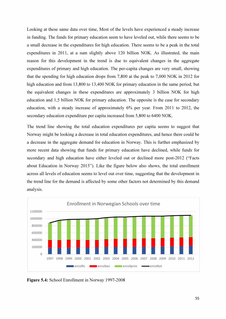
55
Looking at these same data over time, Most of the levels have experienced a steady increase
in funding. The funds for primary education seem to have leveled out, while there seems to be
a small decrease in the expenditures for high education. There seems to be a peak in the total
expenditures in 2011, at a sum slightly above 120 billion NOK. As illustrated, the main
reason for this development in the trend is due to equivalent changes in the aggregate
expenditures of primary and high education. The per-capita changes are very small, showing
that the spending for high education drops from 7,800 at the peak to 7,000 NOK in 2012 for
high education and from 13,800 to 13,400 NOK for primary education in the same period, but
the equivalent changes in these expenditures are approximately 3 billion NOK for high
education and 1,5 billion NOK for primary education. The opposite is the case for secondary
education, with a steady increase of approximately 6% per year. From 2011 to 2012, the
secondary education expenditure per capita increased from 5,800 to 6400 NOK.
The trend line showing the total education expenditures per capita seems to suggest that
Norway might be looking a decrease in total education expenditures, and hence there could be
a decrease in the aggregate demand for education in Norway. This is further emphasized by
more recent data showing that funds for primary education have declined, while funds for
secondary and high education have either leveled out or declined more post-2012 (“Facts
about Education in Norway 2015”). Like the figure below also shows, the total enrollment
across all levels of education seems to level out over time, suggesting that the development in
the trend line for the demand is affected by some other factors not determined by this demand
analysis.
Figure 5.4: School Enrollment in Norway 1997-2008
0
200000
400000
600000
800000
1000000
1200000
1997 1998 1999 2000 2001 2002 2003 2004 2005 2006 2007 2008 2009 2010 2011 2012
Enrollment in Norwegian Schools over time
enrollhi enrollsec enrollprim enrolltot

56
A very important source for the demand for high education is oil related studies among others,
but the sensitivity in other studies will also be affected by performance in the oil sector, and
the oil sector is regarded the most important industry in Norway (Ryggvik, 2010). The value
creation from the oil and gas sector represents approximately 25% of the total GDP in
Norway (ssb.no). Depending on what causes an eventual fall in the performance of the oil
sector, a significant general global decline in the activity of oil and gass could lead to a severe
impact on the Norwegian mainland economy, while an increase in global supply only leads to
a minor decrease in the economy (Bjørnland & Thorsrud, 2014). This goes to show that the
former demand analyses conducted could yield stronger results if there were some kind of
labor market factors involved in the explanation of the education spending ratio.
Figure 5.5: Two Component Aggregate Education Expenditures in Norway
Decomposing the aggregate demand into two different components shows an important
implication for the possible decline in the demand for education. After the liberalization for
the legislation of private and independent schools (lovdata.no), there have been more
significant increases in the demand for private education. However, in the years after the
largest impacts of the global economic crisis, the demand for education funded by the
government in Norway has leveled out and seems to be in the start of a possible decline. Since
the size of the private education is still very small relative to total education expenditures, the
total effect is that there could be a decline in the demand for education after 2011.
0,00
20 000 000 000,00
40 000 000 000,00
60 000 000 000,00
80 000 000 000,00
100 000 000 000,00
120 000 000 000,00
140 000 000 000,00
160 000 000 000,00
1997 1998 1999 2000 2001 2002 2003 2004 2005 2006 2007 2008 2009 2010 2011 2012
Aggregate Education Expenditures, Two Component
govexp privexp totexp

57
Figure 5.6: Two Component School Enrollment in Norway
What can be told when dividing the enrollment into two components? The increase in
enrollment from the start of the time period in 1997 sees an increase in enrollment that
eventually levels out. While there are small increases in the private education enrollment, the
total enrollment numbers for private education have been close to constant both before and
after the liberalization of the private school law in Norway. If the predicted models from the
demand analysis can explain the education spending ratio to some degree, this must mean that
there has been an increase in the price for private education? The estimated inflation-adjusted
price per student for private education confirms this in the figure below. When the enrollment
number is close to constant for private education, the increase in the total education
expenditures for private education is shown by an increase in per-student price for the
provider of education.
Figure 5.7: Two Component Estimation of Inflation-adjusted Price of Education
0
200000
400000
600000
800000
1000000
1200000
1997 1998 1999 2000 2001 2002 2003 2004 2005 2006 2007 2008 2009 2010 2011 2012
Aggregate School Enrollment in Norway, Two Component
enrollg enrolln enrolltot
0
1000
2000
3000
1997 1998 1999 2000 2001 2002 2003 2004 2005 2006 2007 2008 2009 2010 2011 2012
Estimated Inflation-Adjusted Price of Education, Two
Component
Government Private Aggregate

58
Like the correlation analysis of aggregate demand shows, the development of the education
expenditures ratio over time shows that there is some relationship between the expenditure
and the income, but there are some important differences in the fluctuations. The variation is
bigger for the government revenue over time, while the variation is quite low for the private
income. What seems to be an even more important implication when comparing this to the
education spending is that the peak in the spending, and hence the demand to some degree, is
observed earlier in the income data than it is for the changes in education spending. This is an
indication that the income is a leading indicator for the direction of the education funding or
that the education spending is a lagging indicator. The term indicator is relative to the change
in GDP and can either forecast a change in GDP or result in an occurred change in the GDP
(Gottfries, 2013). Gottfries also indicate that employment is a lagging indicator to a shift in
GDP. The comparison in the figure below shows that the government revenue follows the
GDP closely, but is also slightly lagging.
Figure 5.8: Government Revenue and Real GDP per Capita
As a sum of this part of the analysis, there are important differences when comparing the two
components with respect to demand for education and the education expenditure. While the
aggregate education spending shows that there might be a peak and a future decline in this
variable, the government component follows this implication while the private education
spending is increasing. Looking at the demand numbers in terms of enrollment, while there is
a small increase and a peak in accordance to the expenditure data, the increases in these
numbers are very small over time. The enrollment for education funded by the government
0
500
1000
1500
2000
2500
3000
3500
1997 1998 1999 2000 2001 2002 2003 2004 2005 2006 2007 2008 2009 2010 2011 2012
Government Revenue and GDP per capita in
Constant NOK
GDPpercap Govrevpercap

59
seems to have peaked and leveled out for some years, while the demand for private education
is slowly increasing. The increase of cost per-student (in terms of price) for the private
institutions could be a result of the increase in the demand for private education and the
liberalization in legislation, leading to an increase in the establishment of private education
institutions. In general, the corporate decision for education funding and provisioning
(corporate as in government or a private corporation or organization) seems to be a lagging
factor as a result of a change in the economic situation and in enrollment numbers over time.
Still, any suggestions for omitted variable biases seems to suggest that there is at least some
labor market factors that must be included in order to improve the analysis framework when
using this to analyze the demand for education in Norway. Like the data shows from the
research of Bhuller et al. (2011), the returns to schooling in Norway is increasing from 1997
until peaking in 2002, and then declines at a near-constant rate. Comparing this to the data of
education expenditures, there seems to be a negative correlation between the two sides, but
without evidence it is not possible to state whether they actually do behave in the opposite
direction of each other, as the expenditure keeps increasing until peaking in the end of the
time period.
Given the ratio of education spending to real GDP, how much is spent on education compared
to other sectors? The figure below shows an illustration over some of the largest yearly
expenditure items that are funded by the government:
Figure 5.9: Per Capita Government Expenditure, Sector Wise Division
0
50000
100000
150000
200000
250000
1997 1998 1999 2000 2001 2002 2003 2004 2005 2006 2007 2008 2009 2010 2011 2012
Per Capita Government Expenditure
General Public Services Military & Defense Public Safety
Industrial Organization Transportation Environmental protection
Healthcare Education Social Securities
Total per capita

60
Indeed the government expenditures are rising at a nearly constant rate of approximately 6.8%
per year. Social security like age and disability pension plus unemployment compensation are
the largest cost for the government at 407 billion NOK in 2012, or 81,600 NOK per capita,
which constitutes 36.4% of the total public expenditures. The general public services at 46200
NOK per capita include international financial support, public debt transactions,
administration of public administrations at different levels and other services defined as
general public services. The sum of healthcare expenditures per capita is 31,000 NOK in
2012, and education expenditures in 2012 is the fourth largest public expenditure item at
23,800 NOK. Public safety (police, fire departments, courthouses and jails), Military and
defense, industrial organization (agriculture and other natural resource extraction facilities),
and transportation are well below the other expense items, ranging between 4,600 and 18,000
NOK per capita in 2012. Environmental protection has been at a constantly lower level
compared to the other expense items, costing the government just below 300 NOK in 2012.
The given sums and ranking of these have developed over time, and the given time period for
this research shows that social security and general public services have been the two largest
expenditure items throughout this period with small increases every year. In the earlier years
of this period, it is evident that education expenditures were higher than expenditures for
healthcare in Norway. The sudden, significant increase in the health care expenses happened
due to a healthcare reform becoming effect in this time period (Jensen & Bollingmo, 2007).
While this entire time period have seen changes in governance with different priorities within
their budget plans, the expenses within military, public safety, industrial organization and
transportation have only seen smaller increases in their funding, in addition to some cyclical
fluctuations. The greatest increase in any of these was in industrial organization, with a 50%
increase in this item from 2011 to 2012.
While some of the former statistical analyses suggest that there might be signs of a peak in the
Norwegian economy due to a peak in the GDP and a lagging effect in the education spending,
figure 9 illustrates that there still is a steady increase in these expenditures. However, it is still
possible that there could be a peak or a decline in the economy if the government chooses to
maintain the increase in the total expenditure level. This is still possible since possible
changes in the employment rate leads to an increase in the expenditure for social securities.
Since this research does not intend to draw any conclusions about the economic situation in
Norway, the next part in this analysis will try to answer the research questions and the
hypotheses more directly.
61
6. Regression Analysis of Demand for Education
This section will conduct a demand analysis on the background of demand for education and
the government’s education spending. The main purpose of this analysis is to base the
analysis on a model used on a different demography to analyze the same effects estimated in
the original model. In addition, it will also be a test of the model’s applicability showing
whether or not it is possible to use based on data from a different country. As this model has
been used to analyze the effects in China (Chow & Shen, 2006), the outcome will therefore
show if it can be used to analyze these effects in Norway. The applicability could also explain
possible problems with the analysis when used on the population of a different demography,
like omitted variable bias and robustness issues if the output contradicts the theoretical
framework. The amount of data and different categories included might also vary between the
original paper and this research (as one or more categories might be included as opposed to
the other, while some might lack due to availability of data).
6.1.1. Demand Analysis for Three Levels of Education
As explained in the methodology, the analysis is based on equation 40, which implies that
equation 39 is true. The first part of the demand analysis uses this equation to estimate the
income effect and price effect for the different levels of education i, where i = (p,s,h) denotes
the education level (primary, secondary and high education, analyzed separately). First, the
income elasticity is estimated by regressing total education spending for the different levels
for education (divided by an appropriate population number) on real income per capita in
Norway, using cross regional data of 2012. As numbers for quality-adjusted enrollment for
the different regions is not available in Norway, this analysis will also transform the cross-
sectional analysis into a time series analysis when estimating the price effect. The variable ln
qia is constructed as shown by equation 41, where the estimated coefficient of income
elasticity is inserted in ln qia. This constructed variable is used in the time series analysis by
the regression of the price effect on the income-adjusted log quantity (income adjusted
demand). The output of this regression will yield the inverse of the price effect, where the
regression of income-adjusted log quantity on the log price effect could determine any
possible bias in the estimated inverse elasticity. The following table shows the estimates from
the conducted regression for all three levels of education:

62
Table 6.1: Total Expenditures for Primary Education
Explanatory Variable: Coefficient Value: Standard Error: T-value:
Intercept of ln pq 6.508 2.256 2.884 (0.014)
Income elasticity -0.252 0.286 -0.881 (0.395)
Intercept of ln qia 0.492 0.493 0.996 (0.487)
Price elasticity -0.051 0.083 -1.283 (0.547)
- With F-value equal of 0.777 for the income test and 0.382 for the price test, neither of
the hypothesis tests are significant. From the total sums of squares equal to 0.808 and
0.037, the respective residual sums of squares are 0.759 and 0.036.
As table 6.1 shows, the income elasticity is negative and small, and the size of the price
elasticity, derived from the income-adjusted log quantity of enrollment, is also very small. For
this regression, a total of five outliers have been removed because of preliminary testing
showing that the inclusion of these data resulted in output signaling a very poor fit to the
dependent variable. While this table shows a positive number for the price elasticity, this
number is negative after being inserted into its relevant equation. In other words, ln qia is
equal to the constant minus the price effect, so the correct value for the price elasticity is -
0.051, indicating that there is a small, negative price elasticity.
A second way of estimating the price elasticity is by regressing ln p on ln qia, the opposite of
what has been reported. By reversing the variables and changing which one is the dependent
and explanatory variable, the inverse estimate of price elasticity can show whether there is a
possibility of a bias when computed to a proper estimate by assuming that the coefficient of ln
qia must be equal to 1. From the inverse estimate, the price elasticity in this case is -1.93, thus
showing that there could be a presence of a significant bias of simultaneity in this estimate
due to the great difference between the two estimates of the same variable.
Table 6.1 also shows that both the income and price elasticity are insignificant or weakly
significance. The income elasticity would show a possible contradiction of the predictions of
hypothesis 1 when being negative rather than positive, as a positive (negative) percentage
shift in income would lead to a negative (positive) shift in education spending, suggesting that
education might be inferior. However, there is not enough evidence to reject the null
hypothesis of perfect inelasticity, and therefore this OLS estimation cannot prove that income
does have an effect on the total education expenditures in Norway.

63
The same outcome is yielded when examining the price effect. This estimation already suffers
both from the income effect being insignificant when assuming that the size of the dependent
variable from equation 43 depends of the size of the income effect, and also because of the
two different methods of estimating the price effect results in two different values of
elasticity. In addition, neither of the two estimates are found to be significant, with the
regression of price on the income-adjusted log enrollment having a standard error of 0.835
and a t-value of 0.618. Therefore, there is not enough evidence to reject the null hypothesis
for the estimation of price elasticity for primary education no matter which one of the two
methods of estimation being conducted.
Table 6.2: Total Expenditures for Secondary Education
Explanatory Variable: Coefficient Value: Standard Error: T-value:
Intercept of ln pq 7.183 1.217 5.904*** (0.00)
Income elasticity -0.427 0.154 -2.773** (0.013)
Intercept of ln qia 0.142 0.538 0.264 (0.796)
Price elasticity -0.033 0.082 0.405 (0.692)
** Significant at the 5% level
*** Significant at the 1% level
- With F-value equal of 7.689 for the income test and 0.164 for the price test, only the
income test is significant. From the total sums of squares equal to 0.503 and 0.037,
the respective residual sums of squares are 0.759 and 0.036.
The output for secondary education shows that the income elasticity has a negative sign, and
the size of the elasticity is somewhat bigger than in the case of primary education. This OLS
estimation does not exclude any of the Norwegian counties as outliers. Comparing
furthermore to the primary education case, the evidence for inferiority of education is also
stronger for secondary education, and the absolute t-value suggests that this is statistically
significant at the 5% level. Concerning the price effect, the elasticity is estimated to be -0.033,
once again showing a small, negative effect.
In this case, there is a statistically significant income effect, but the following estimation of
price elasticity of secondary education is insignificant through its t-value. An additional test
of a possible bias in this estimate is done by regressing ln p on ln qia, where the inverse
estimate results in an estimate for the log price being -2.86, showing the possibility of a large
bias due to simultaneity. Additionally, the difference between these and their respective
significance shows that neither of these effects are sufficiently evident, as the latter estimation

64
with the price of secondary education being the dependent variable has a standard error of
0.861 and a t-value of 0.405. Therefore, there is not enough evidence to conclude that there is
a negative income effect or a small, negative price effect when analyzing the total expenditure
on secondary education.
Table 6.3: Total Education Expenditures for High Education
Explanatory Variable: Coefficient Value: Standard Error: T-value:
Intercept of ln pq 0.880 4.014 0.219 (0.830)
Income elasticity 0.282 0.512 0.551 (0.592)
- With F-value equal of 0.304 for this hypothesis test, this test is not significant. From
the total sum of squares equal to 0.948, the residual sums of squares is 0.925
This output is given from the demand analysis of total education expenditures for high
education, aggregating the government and private components that will be separated in the
next part of the analysis. This analysis does exclude some outliers, where preliminary analysis
shows that these do have an impact on the outcome of this analysis. An important difference
from the former analyses is that only the income effect is estimated here, to be compared to
the outcome of a two-component time series analysis of high education following this
analysis.
However, this elasticity cannot be used for comparison as the OLS estimation of the income
effect shows that the independent variable is not significant. This time, the income elasticity is
positive (but small), but this is not relevant as the regression yields an insignificant estimate
for the income elasticity. There is not enough evidence to reject the null hypothesis, and
therefore this estimation does not prove that the coefficient value is an unbiased best estimate
of the income elasticity.
To summarize the analysis of the three levels of education, estimation of the income and price
elasticities is conducted by first estimating the income effect by the use of cross-regional data
from Norway, while this yielded estimate is plugged into equation 43 to estimate the price
effect. For the first two levels of education, only the negative income elasticity from the
secondary education is sufficiently significant. There could be various reasons for this specific
part of the empirical model not being applicable for the Norwegian data.

65
From the output of the analyses conducted, there are many factors that suggest issues with the
applicability of OLS estimation for this model. Various indicators show that the goodness-of-
fit for the estimated elasticities cannot possibly be the unbiased best estimates, even when the
income elasticity of secondary education is not perfectly inelastic. Looking at the R-squared
from the various tests, the ratio is between 0.012 and 0.31. Wooldridge (2009) explains that
the R-squared ratio how much of the sample variation in the dependent variable that is
explained by the explanatory variables. When the R-squared ratio is close to 1, the OLS
estimation provides a perfect fit. The concern with this model is that the highest R-squared is
0.31, which states that the OLS line fits 31% of the data. With most numbers around 10% or
below, the OLS estimators show that the goodness-of-fit is very low, and the insignificance of
most numbers are therefore, hence the resulting insignificance or weak significance in both
the hypothesis tests and the estimated elasticities. This raises additional concern around the
applicability of the negative income elasticity of secondary education.
Why does this happen? One of the most obvious reasons, especially due to the many
configurations of equations into single variable tests, is that most of these OLS estimations
would suffer from the omitted variable bias. Even though the variables are put into context
with a regression equation with at least two explanatory models, each of the estimations for
obtaining values of elasticity is conducted with only one explanatory variable. The main
problem with a simple regression analysis is that it violates the ceteris paribus, and it is not
possible to state that a change in y happens because of a change in x when y also depends on
other factors. This is a very bold statement claiming that one effect can explain a change in a
dependent variable while being uncorrelated to all other variables absorbed in the residual (as
income is assumed uncorrelated to price without being testable without quality-adjusted
enrollment for each region).
Conducting ANOVA-tests for all OLS regressions, there are reasons for more concern. As all
of these tests show, the variance explained by the regression is quite low. The number of the
residual is well above 50% for all of the ANOVA-tests, suggesting that most of the variance is
explained in the tests’ estimated error term rather than explained by the regressions. While a
lot of these tests also yield low F-statistics, the tendencies are very clear when comparing to
the low values of R-squared. Since this evidence states that there is a violation of ceteris
paribus because of an omitted variable bias (%� ≠ 0��67� ≠ 0in a simple regression model
with one explanatory variable), the estimated elasticities are not unbiased best estimates for
the actual phenomenon. An omitted variable bias leads to a bias in the estimated elasticities,

66
and the sign and size of the omitted variable depends on the variable(s) that has (have) been
omitted (Wooldridge, 2009, 91). There are signs of this in the price elasticities of primary and
secondary education, but there is not sufficient evidence to determine this as all of these
estimates are insignificant.
Another important factor to determine whether or not the estimates from the regressions are
unbiased best estimates is to test for multicollinearity. Under the Gauss-Markov theorems for
unbiased estimates in time series analysis, none of the independent variables are allowed to
perfectly correlate with each other. This does not mean that the explanatory variables are not
allowed to correlate with each other, but additionally to perfect correlation they are not
allowed to correlate strongly with each other. If they do, multicollinearity would be present in
the estimation. This is not possible to test due to scarce cross-regional data about the quality-
adjusted enrollment for primary and secondary education that is available. Instead, correlation
tests can be conducted in order to examine the correlation between independent and
explanatory variables. Testing for heteroscedasticity shows that all of the variables are
homoscedastic. Conducting a Breusch-Pagan test of heteroscedasticity yields BP-statistics
between 0 and 1.03, and the p-values from the tests indicates that none of the two-step
analyses exhibits heteroscedasticity.
Correlation values shows that for the income effect, the total education expenditures for
secondary education and the income per capita are correlated but opposite (-0.558), while the
income has a low correlation with the expenditure for primary and high education (-0.247 and
0.157 respectively). There are signs of an opposite linear relation between secondary
education spending and income per capita, while there is no linear relationship between
income per capita and education spending for primary and high education. The same
phenomenon passes on to the estimation of price elasticity of education (where the time series
analysis of high education is omitted). The estimated price elasticities are almost uncorrelated
to their respective income-adjusted demand functions, at 0.163 and 0.108 respectively. For
both effects, this shows strong signs for an omitted variable bias, which is a violation of a
simple regression model being sufficient to yield best linear unbiased estimates for the
Norwegian education spending and demand for education at all three levels of education. The
conclusion is that there is not enough to confirm or reject hypothesis 1; it is not possible to
prove that income and price have any effect on the education spending in Norway.
67
6.1.2. Two Component Time Series Analysis of High Education
After the two-step analysis has been conducted for all three levels of education, the following
time series analysis divides the demand for high education into two components:
governmentally funded and privately funded education. High education is the only level being
divided into two components because this level of education has the highest number of private
schools and enrollment rate of all education levels in Norway. Nevertheless, the definition of
a private school is not a unified definition as it consists of both private schools and
independent schools. As stated in the methodology, private schools were forbidden in Norway
until a change in legislation starting in 2005, but independent schools (a majority of these
being religious) were permitted before this. Because of this, publicly available information
about these private institutions have been very limited, and the limitation in detailed
information about quality-adjusted enrollment and expenditures have therefore been estimated
in years before 2005 and after 2009.
The time series estimation has the ratio of total demand for high education in Norway divided
by the population number each year as dependent variable. As of equation 43, the explanatory
variables are the income and price elasticities for the government and private component
aggregated into one time series analysis. The income for the government component is
defined as the inflation-adjusted government revenue per capita, while the price effect is the
ratio of government expenditure for high education over enrollment and CPI. For the non-
government component, the income is defined as real GDP per capita (more specifically the
inflation-adjusted real GDP per capita), while the appropriate per-student price for private
education is defined as the expenditure for private educational institutions over enrollment
and CPI. Another important note about private educational institutions is that most of these
are eligible to receive funds from the government, to be used for the operation of the facility
only (capital transfers of these funds like dividends are prohibited by law).
The time series analysis is not only chosen because of the availability of enrollment numbers,
but also due to the lack of best linear unbiased estimates from cross-regional and time series
analysis from the former analysis. This time series analysis examines if a pure time series
analysis with the explanatory variables of two components will have any effect on the omitted
variable bias. The following estimates are gathered from this analysis:

68
Table 6.4: Two Component Analysis of Expenditure for High Education
Explanatory Variables
(coefficient values and
standard error)
Intercept ln yg ln pg Ln yn Ln pn
-0.783
(2.229)
0.178**
(0.064)
-0.007
(0.130)
-0.453
(0.276)
0.021
(0.046)
Intercept Ln yg Ln pg Ln yn
-0.45
(2.040)
0.183**
(0.061)
0
(0.125)
-0.510*
(0.239)
Intercept Ln yg Ln yn Ln pn
-0.715
(1.790)
0.181***
(0.028)
-0.459*
(0.247)
0.021
(0.044)
* Significant at 10% level
** Significant at 5% level
*** Significant at 1% level
The outcome from the table is based on three different configurations of the regression. The
first row shows the estimates when all of the independent variables are included (the time
series not exclude any outliers from any part of the analysis). The next two rows exclude one
of the two price variables, as they both are insignificant. At least one of them is included in
order to try to avoid a possible omitted variable bias by only including the income effects.
Starting with the original outcome from the time series analysis, the elasticities from
government component can be interpreted as an expected outcome from the relevant
hypothesis. The income elasticity is small and positive, while the price elasticity of education
is very small and negative. The non-government component yields a negative income effect
and a positive price effect.
Since both of the price effects are not significant (t-values of 0.056 and -0.464 for the
government and non-government elasticity respectively), additional regressions are conducted
in order to observe the eventual changes in the estimates when one of the insignificant effects
are removed from the regression equation. As seen in table 5.4, including the price effect of
education funded by the government could result in a perfectly inelastic demand for high
education, ceteris paribus, but this estimate is strongly insignificant (t-value of 0.003) when
the non-government price effect is omitted. Another regression is conducted, including the
price effect for the non-government component. The small changes in each estimate of
elasticity shows that the inclusion of the government price effect has no real effect on the
estimates, which means that this variable should be a part of the residual. While the exclusion

69
of either price effect yields greater significance for the estimated income elasticities, the same
change for the price effects are very small and is still insignificant (t-value of -0.481). There is
not enough evidence to reject the null hypothesis for any of the price effects, no matter which
one of them are included or omitted.
Configurations of equation 43 yield significant values for the government income effect, and
this is also confirmed when the omission of any price variable leads to very small changes in
the income elasticity. In the first regression and the second regression, the estimated
government income elasticity is significant at the 5% level (t-value of 2.777 and 3.002), and
omitting the non-government price effect leads to a change in the income elasticity estimate
from 0.178 to 0.183. Omitting the government price effect yields an estimate that is
significant at the 1% level, and the marginal change indicates that evidence can confirm a
small and positive income elasticity that is slightly above 0.180 (t-value of 6.387). Ceteris
paribus, a 1% change in government revenue per capita results in a 0.18% change in the
demand for high education.
Examining the change in the income effect for the non-government component sees the
elasticity change from a non-significant value in the original regression (t-value of -1.641) to
an estimate that is significant at the 10% level when at least one of the price variables are
omitted (t-value of -2.129 when non-government price of education is omitted and -1.853
when the government price is omitted). The sign of the estimate shows that a 1% change in
the GDP per capita leads to a considerable opposite change (45-51%) in the demand for high
education. The significance of this estimate shows that there is limited evidence that the
demand for education is an inferior good if and only if the non-government income changes,
ceteris paribus.
When further testing the OLS estimators by omitting all price variables, the income elasticity
for the government component remains at 0.183 and is significant at the 1% level (t-value of
6.713), and the income elasticity for the non-government component is now also significant at
the 1% level, the elasticity now being -0.51 (t-value of -2.349). Adding the results from the
ANOVA-tests and the R-squared from each of the regressions conducted, the ANOVA states
that a total sum of squares at 0.34 is explained by the regression sum of squares at 0.27 and
the residual sum of squares at 0.08. Therefore, the majority of variation from the estimated
model is explained by the regression, limiting the possibility of an omitted variable bias.

70
This is reflected in the R-squared, which is equal to 0.776 when omitting the non-government
price effect and by omitting all price effects, while the R-squared is equal to 0.781 for the
original regression and when the government price effect is omitted. The fit of the estimated
elasticities is between 77.6% and 78.1% for the regressed OLS line. This leads to the
goodness-of-fit being quite strong. However, testing the correlation for the entire equation
shows that there could be multicollinearity as the government income effect and price effect
correlates (correlation of 0.875). Assuming that this is false when the price variables are
omitted, there is a strong correlation between the total demand for high education (0.825), but
there is almost no correlation between the demand for high education and the non-government
income. Testing for heteroscedasticity shows that all BP-statistics between 0.42 and 4.66
(lowest p-value being 0.27) does not prove any heteroscedasticity being present in any of the
configurations when estimating the demand for high education.
Therefore, the evidence suggesting inferiority for the demand for education with respect to the
private income effect, ceteris paribus, but this effect is uncertain both because of insufficient
statistical evidence from the OLS regression and because the dependent variable is weakly
correlated to the total demand for education. Hypothesis 2 can only be confirmed for the
government income effect, while there are not enough evidence to confirm or reject this
hypothesis with respect to any of the other explanatory variables. In other words, there is a
small and positive income effect suggesting that an increase in the income level in Norway
leads to an increase in demand for high education. However, this analysis is not able to
sufficiently prove that there is a real effect between the demand for education and private
income. There is no evidence that the price variables have any effect on the demand for high
education.
6.1.3. Aggregate Demand
With the results from the former analyses in mind, the income effect and price effect will now
be tested to examine if they can explain the aggregate demand for education. This is derived
through the expression total aggregate education expenditure for all levels of education over
real GDP, as shown in equation 44. This analysis is also divided into two parts, where the first
part uses equation 44 to perform a two-step analysis, estimating the aggregate income
elasticity by using cross-regional data and the price elasticity from time series data. The
second part conducts a time series analysis based on equation 47, where the dependent

71
variable is the total aggregate expenditure over GDP, with income and price effect as
explanatory variables.
The outcome from the regressions is afterwards plotted, which will clearly show the
goodness-of-fit for each of the methods used compared to the real numbers. While the time
series analysis of the total expenditure over GDP yields a prediction of the real ratio, the
estimates obtained from the two-step analysis provides fitted values that will be inserted into
equation 44. The two-step analysis will also be split in two, where the estimated income
elasticity remains constant for both of these additional parts, while the price elasticity is
estimated first by regressing ln qia on ln p, and finally ln p is regressed on ln qia to obtain an
inverse estimate that through rearrangement can yield an estimate that will determine whether
there is a possible bias in the price elasticity. The following table shows the outcome of the
two-step and time series analysis:
Table 6.5: Aggregate Demand Analysis, Two-step and Time Series
Estimation: Constant: Income Elasticity: Constant (two-step
time series)
Price Elasticity:
Two-step 2.273
(1.650)
0.369*
(0.209)
-7.154***
(0.389)
-0.424***
(0.059)
“” 2.273
(1.650)
0.369*
(0.209)
14.67***
(1.132)
-0.54***
(0.259)
Time Series -4.188**
(1.792)
0.238***
(0.225)
- -0.121***
(0.053)
*Significant at the 10% level
** Significant at the 5% level
***Significant at the 1% level
The conducted analysis on aggregate demand shows some important differences from the
former analyses. Even if some of the analyses have shown signs of consistency with the
predicted effects, the aggregate demand analysis yields estimated elasticities that are
consistent with the predictions in hypothesis 4, no matter the use of the two-step method or
the time series.

Figure 6.1: Aggregate Demand
The two-step method, yields positive income elasticity, while the price elasticity is estimated
to be negative. If the two-step
income and price effect, there could be more considerable changes in the education spe
when any of the effects changes. The income effect is significant at the 10% level, meaning
that there is some evidence for this income elasticity being applicable. Comparing the two
different estimated price effects shows that the small difference b
in a smaller chance for a bias being present in this estimate, and the estimated price elasticity
is strongly significant. To compute the fitted values when comparing to the real numbers, the
appropriate estimate of price elast
hence b = -0.454.
Estimating the ratio of total education
that are consistent with hypothesis
elasticity is negative. Both estimates are significant at the 1% level, suggesting that there is
strong evidence to confirm the hypothesis. Further tests are, however, necessary in order to
confirm that both tests exhibit
conducted, the lacking goodness
is 0.155 for the cross-regional regression and 0.785 for both of the price elasticity estimations.
While the goodness-of-fit seems to be stronger for the price estimation, the use of the
insignificant income elasticity used in the estimation of the price elasticity means that its
goodness-of-fit cannot be considered true. Due to the lack of an aggregate quality
enrollment in the cross-regional data, it is not possible to test for multicollinearity
-3,5
-3
-2,5
-2
-1,5
-1
-0,5
0
1997
1998
1999
2000
2001
Ag
gre
ga
te E
du
cati
on
Sp
en
din
g t
o
GD
P
emand Compared to the Two-step and Time Series
yields positive income elasticity, while the price elasticity is estimated
step analysis can yield the best linear unbiased estimates for the
income and price effect, there could be more considerable changes in the education spe
when any of the effects changes. The income effect is significant at the 10% level, meaning
some evidence for this income elasticity being applicable. Comparing the two
different estimated price effects shows that the small difference between the estimates results
in a smaller chance for a bias being present in this estimate, and the estimated price elasticity
is strongly significant. To compute the fitted values when comparing to the real numbers, the
appropriate estimate of price elasticity is the one obtained from the first entry in table 5
Estimating the ratio of total education spending to GDP through time series yields elasticities
that are consistent with hypothesis 4, where the elasticity of income is positive
elasticity is negative. Both estimates are significant at the 1% level, suggesting that there is
ence to confirm the hypothesis. Further tests are, however, necessary in order to
exhibit valid evidence. In comparison to former two
conducted, the lacking goodness-of-fit for this model is confirmed by their R
regional regression and 0.785 for both of the price elasticity estimations.
seems to be stronger for the price estimation, the use of the
income elasticity used in the estimation of the price elasticity means that its
fit cannot be considered true. Due to the lack of an aggregate quality
regional data, it is not possible to test for multicollinearity
2001
2002
2003
2004
2005
2006
2007
2008
2009
2010
2011
2012
Aggregate Demand
72
eries Estimation
yields positive income elasticity, while the price elasticity is estimated
analysis can yield the best linear unbiased estimates for the
income and price effect, there could be more considerable changes in the education spending
when any of the effects changes. The income effect is significant at the 10% level, meaning
some evidence for this income elasticity being applicable. Comparing the two
etween the estimates results
in a smaller chance for a bias being present in this estimate, and the estimated price elasticity
is strongly significant. To compute the fitted values when comparing to the real numbers, the
from the first entry in table 5.5,
ough time series yields elasticities
where the elasticity of income is positive and the price
elasticity is negative. Both estimates are significant at the 1% level, suggesting that there is
ence to confirm the hypothesis. Further tests are, however, necessary in order to
mer two-step analyses
fit for this model is confirmed by their R-squared, which
regional regression and 0.785 for both of the price elasticity estimations.
seems to be stronger for the price estimation, the use of the
income elasticity used in the estimation of the price elasticity means that its
fit cannot be considered true. Due to the lack of an aggregate quality-adjusted
regional data, it is not possible to test for multicollinearity or for any
2012
73
correlation at all, but a correlation test between the total education spending and the real GDP
per capita shows that there is a low correlation between them (0.394).
Just like the figure shows, there is a much stronger goodness-of-fit between the predicted
model from the time series of the spending to GDP ratio. To confirm this, the hypothesis test
based on this estimation reveals and R-squared at 0.972, so the hypothesis test finds a very
strong goodness-of-fit to the actual ratio. While the former two-step analysis suggests that
there could be an omitted variable bias as the value of the residual sum of squares is estimated
to be quite high, this time series prediction of the ratio directly suggests that the chance for an
omitted variable bias is very low (residual sum of squares at 0.010 of total sum of squares
equal to 0.347). Checking for multicollinearity reveals that the aggregate income and price
effect is almost perfectly uncorrelated with each other (0.08), but it also reveals a strong
correlation between the dependent variable and the price effect plus a weak and negative
correlation between the dependent variable and the income elasticity. Once again this
provides some evidence that the education expenditure is not very dependent on income in
Norway, but the evidence from this time series regression is strong and robust enough to
confirm hypothesis 4. Breusch-Pagan tests shows that there are some signs of
heteroscedasticity for the two-step time series analysis (p-value of 0.17), but this is not
sufficient to reject homoscedasticity.
The analysis shows that the two-step analysis cannot tell us whether income and price have
any effect on the education spending in Norway. The time series analysis shows that income
has a small and positive effect while the price has a small and negative effect on the education
spending. This is consistent with hypothesis 6 and shows that education in Norway is a
normal good. Education spending in Norway increases relative to real GDP increases by
23.8% when there is a 1% increase in income, and the same spending to GDP ratio decreases
12.1% when there is a 1% increase in the aggregate price of education.
6.1.4. Aggregate Demand: Two-step, Two Component Analysis
Further analysis of the aggregate demand sees to divide to the education spending into two
different components. Splitting aggregate demand into a government and a private component
makes it possible to examine the impact of the elasticities on their respective income and price
effects. The analysis is divided in two, by using two different methods for both the
government and the private component. The first method is OLS estimation through the two-
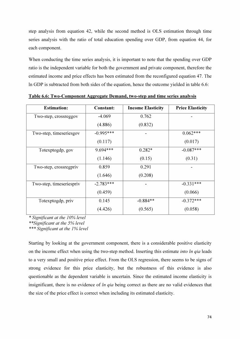
74
step analysis from equation 42, while the second method is OLS estimation through time
series analysis with the ratio of total education spending over GDP, from equation 44, for
each component.
When conducting the time series analysis, it is important to note that the spending over GDP
ratio is the independent variable for both the government and private component, therefore the
estimated income and price effects has been estimated from the reconfigured equation 47. The
ln GDP is subtracted from both sides of the equation, hence the outcome yielded in table 6.6:
Table 6.6: Two-Component Aggregate Demand, two-step and time series analysis
Estimation: Constant: Income Elasticity Price Elasticity
Two-step, crossreggov -4.069
(4.886)
0.762
(0.832)
-
Two-step, timeseriesgov -0.995***
(0.117)
- 0.062***
(0.017)
Totexptogdp, gov 9.694***
(1.146)
0.282*
(0.15)
-0.087***
(0.31)
Two-step, crossregpriv 0.859
(1.646)
0.291
(0.208)
-
Two-step, timeseriespriv -2.783***
(0.459)
- -0.331***
(0.066)
Totexptogdp, priv 0.145
(4.426)
-0.884**
(0.565)
-0.372***
(0.058)
* Significant at the 10% level
**Significant at the 5% level
*** Significant at the 1% level
Starting by looking at the government component, there is a considerable positive elasticity
on the income effect when using the two-step method. Inserting this estimate into ln qia leads
to a very small and positive price effect. From the OLS regression, there seems to be signs of
strong evidence for this price elasticity, but the robustness of this evidence is also
questionable as the dependent variable is uncertain. Since the estimated income elasticity is
insignificant, there is no evidence of ln qia being correct as there are no valid evidences that
the size of the price effect is correct when including its estimated elasticity.
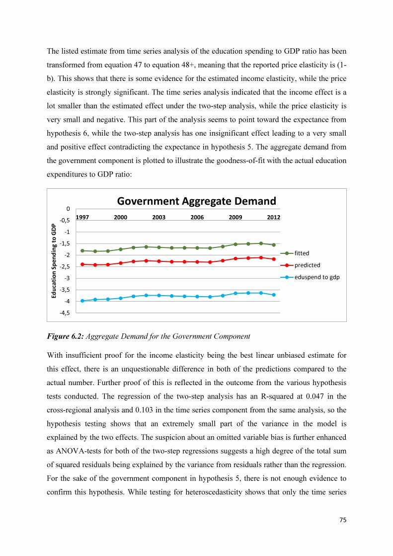
75
The listed estimate from time series analysis of the education spending to GDP ratio has been
transformed from equation 47 to equation 48+, meaning that the reported price elasticity is (1-
b). This shows that there is some evidence for the estimated income elasticity, while the price
elasticity is strongly significant. The time series analysis indicated that the income effect is a
lot smaller than the estimated effect under the two-step analysis, while the price elasticity is
very small and negative. This part of the analysis seems to point toward the expectance from
hypothesis 6, while the two-step analysis has one insignificant effect leading to a very small
and positive effect contradicting the expectance in hypothesis 5. The aggregate demand from
the government component is plotted to illustrate the goodness-of-fit with the actual education
expenditures to GDP ratio:
Figure 6.2: Aggregate Demand for the Government Component
With insufficient proof for the income elasticity being the best linear unbiased estimate for
this effect, there is an unquestionable difference in both of the predictions compared to the
actual number. Further proof of this is reflected in the outcome from the various hypothesis
tests conducted. The regression of the two-step analysis has an R-squared at 0.047 in the
cross-regional analysis and 0.103 in the time series component from the same analysis, so the
hypothesis testing shows that an extremely small part of the variance in the model is
explained by the two effects. The suspicion about an omitted variable bias is further enhanced
as ANOVA-tests for both of the two-step regressions suggests a high degree of the total sum
of squared residuals being explained by the variance from residuals rather than the regression.
For the sake of the government component in hypothesis 5, there is not enough evidence to
confirm this hypothesis. While testing for heteroscedasticity shows that only the time series
-4,5
-4
-3,5
-3
-2,5
-2
-1,5
-1
-0,5
0
1997 2000 2003 2006 2009 2012
Ed
uca
tio
n S
pe
nd
ing
to
GD
P
Government Aggregate Demand
fitted
predicted
eduspend to gdp

76
shows sign of heteroscedasticity, all of the government models exhibit homoscedasticity.
However, with low or no significance in the income effects, the use of the reconfigured
equation 48 to determine the price elasticity makes it impossible to conclude that the evidence
shows a true price elasticity estimate.
Comparing this to the time series analysis of the education spending to GDP ratio from
equation 47, the R-squared and the ANOVA-test suggests a much stronger fit to the actual
model, with an R-squared equal to 0.925, and a total sum of squared residuals at 0.506 only
being explained by a residual sum of squares at 0.038. Transforming this time series analysis
into equation 48 does not show the same effect, as it cannot be used to explain the actual ratio.
Because of the reconfigured equation being constructed to also be dependent of the
government income effect through subtraction of this, using an estimated income elasticity
that has not be proven to be a best estimate might lead to a weakness when predicting an
actual phenomenon. While reconfiguring the dependent variable, the real GDP is now
included in the right hand side of the equation, but is constant while the price effect is variable
with respect to its elasticity. Therefore, the government component of hypothesis 6 cannot be
fully confirmed as there is strong evidence for the price elasticity being a best linear unbiased
estimate, but there is only limited proof due to the income elasticity leading to a poor
goodness-of-fit when plugged into the reconfigured expenditure to GDP ratio for the
government component.
For the private component, the outcome of the two-step analysis is similar to the outcome
from the government component. There is a small and positive income effect from the use of
cross-regional data, while there is negative price elasticity from the time series part. In
general, the strength of the evidence is also very similar as the income elasticity is
insignificant, while the price elasticity is significant all the way to the 1% level. However, this
proof is as questionable as from the two-step analysis of the government component when
using an insignificant estimate to obtain a significant estimate of a different effect.
Nevertheless, figure 2 shows that there is a very poor goodness-of-fit, meaning that the two-
step analysis cannot be used to explain the aggregate education expenditure to GDP ratio for
private education. As a sum of this, there is not enough evidence to conclude that hypothesis 6
is true. It is therefore not possible to reject the chance of both income and price being
perfectly inelastic.
The time series analysis of the aggregate private education expenditures over GDP seems to
exhibit some strong, but opposite results of what has been predicted in hypothesis 6. First, the

77
income elasticity is negative and quite large compared to any other of the elasticities
estimated so far, but the price elasticity is also negative and more modest in size. To be able
to possibly confirm this, this prediction must be consisted with the real values, all plotted in
the figure below:
Figure 6.3: Aggregate Demand for the Private Component
Figure 6.3 suggests a strong goodness-of-fit between the predicted model and the actual ratio
computed. Examining this closer reveals that there is a very high R-squared value for this
OLS estimation, suggesting that the predicted model fits the real ratio at 97.7%, and the
residual is also assumed very small as the ANOVA test predicts that the residual only explains
0.059 of a total sum of squares of 2.577, also suggesting that there is a very low chance for an
omitted variable bias. To confirm that these estimated are the best linear unbiased estimates,
the estimated variables must also be tested for possible heteroscedasticity and
multicollinearity. The Breusch-Pagan test reveals that both of the two-step analyses and the
time series analysis of the spending to GDP ratio is homoscedastic.
A correlation test of all three variables involved in this part reveals that there is no
multicollinearity between the income effect and price effect. However, the test reveals that
there is an almost perfect correlation between the education spending to GDP ratio, but this
dependent variable is hardly correlated with the income effect. Considering that the income
elasticity suggests that income is inferior with a substantial change to education spending
when the GDP per capita increases (holding the price effect constant) this proof might be
considered true, but the low impact it has on the education spending must be taken into
-7
-6
-5
-4
-3
-2
-1
0
1997 2000 2003 2006 2009 2012
Ed
uca
tio
n S
pe
nd
ing
to
GD
P
Private Aggregate Demand
fitted
predicted
eduspend
to gdp
78
consideration. Additionally, further testing must be conducted over a long time period in order
to prove that there is indeed inferiority when holding the price effect constant. In regards of
hypothesis 6, the evidence can is sufficient to reject this hypothesis concerning the income
effect, while it can be confirmed for the private education price effect. It is not possible to
collectively confirm or reject the hypothesis. However, the strong evidence for the price
effects for both components confirms hypothesis 6 with respect to the price effect, which is
also a confirmation that the demand for private education is more sensitive to a change in
price than the demand for education funded by the government. Examining the results, the
negative impact on the income effect followed by a smaller negative impact in the price effect
suggests that the education spending to GDP ratio will decrease as income increases, and the
same happens with an increase in price. Following this ratio closely over time will tell if this
is true.
To summarize the two component aggregate demand analyses, none of the two-step analyses
proves that the elasticities found are applicable as fitted numbers to the education spending to
GDP ratio. This means that this research cannot prove the impact of income and price on the
education spending in Norway. Evidence shows that there is a relationship between the
dependent and the independent variables, but there are not sufficient evidence to claim that
the income elasticity is true. This leads to a very poor fit to the real model, and the conclusion
is that it is not possible to prove the impact that the income has on the education spending to
GDP ratio, while the evidence suggests that the price of public education has a small and
negative effect on the same ratio. The private education component shows that both income
and price has a negative effect on the demand for private education. This evidence suggests
that private education in Norway is an inferior good, but not a Giffen good.
6.2. Testing for Fixed Effects and Random Effects
After looking at the various results from the regression analyses, this section will examine if
the different results depend on variation across time and across components like region and
source of funding. From the methodology part 4.1.1, Torres-Reyna (2007) gives a general
explanation that fixed effects when the tester is only interested in analyzing the impact of
some variables that vary over time. Fixed effects testing through equation 46 removes time-
invariant characteristics to assess the net effect of the explanatory variables on the outcome
variable. For random effects, variation across entities is assumed to be random and
uncorrelated with the explanatory variables. In addition to time-variant characteristics,
regression with random effects can be conducted by using equation 49.

79
To reveal if there are fixed effects or random effects in the regression framework used for this
thesis, various tests can be conducted to reveal if the regressions exhibit random or fixed
effects. In general, the tests conducted with the results listed in table 6.7 will first conduct a
fixed effects test on a regression from a relevant two-step or a time series analysis. Following
this regression, an F-test will be conducted to determine if there is a significant probability of
fixed effects being present in the regression. The null hypothesis will be that there is no fixed
effect. To further control for the possibility of random effects, a pooling OLS regression will
be added. The outcome from the pooling regression will be inserted into a Breusch-Pagan
Lagrange Multiplier test for random effects. Table 6.7 reveals the outcome from the F-test of
fixed effects and the Breusch-Pagan of random effects with further explanation of the results
below:
Table 6.7: Fixed and Random Effects
Entity for Hypothesis Testing: Fixed Effects F-test
F
Random Effects BP-test
χ²
Cross-regional Expenditure, All 63.811 (0.000)*** 228.345 (0.000)***
Time Series Expenditure, All 1902.912 (0.000)*** 211.760 (0.000)***
Time Series High Education 238.565 (0.000)*** 0.672 (0.413)
Time Series Aggregate Demand 8793.943 (0.000)*** 36.309 (0.000)***
*** Significant at the 1% level
The regressions used for these tests are not all the same as used above. The cross-regional and
time series total expenditure pq are aggregated across all levels of education to check for
random effects when using income and price as explanatory variables with the three levels of
education as components for each region or year. The time series analysis of high education
and the aggregate demand uses the government and private education as separate components
for each year. All regressions uses the total education expenditure pq as the dependent
variable for these estimations and tests. The income-adjusted log quantity of demand for
education is not relevant as none of the two-step analyses are included for fixed and random
effects testing. Instead of using the education spending to GDP ratio when the government
component yields valid results for the total spending but not for the ratio, the total education
expenditure is the dependent variable of choice. All of the estimations use income and price
(for different levels of education and sources of funding) as explanatory variables.

80
The results from table 6.7 shows that only the time series analysis of high education exhibits
no sign of random effects. The Breusch-Pagan test of the pooling regression shows that there
are no significant differences across the government and private components, therefore OLS
estimation can be used. (Torres-Reyna, 2010) With all of the other entities exhibiting possible
presence of both fixed and random effects, a Hausman test must be conducted to determine
what kind of estimation that is appropriate for each entity of analysis.
Table 6.8: Hausman Test of Fixed and Random Effects
Entity for Hausman Test Hausman χ² p-value
Cross-regional Expenditure, All 0.041 0.980
Time Series Expenditure, All 0.151 0.928
Time Series Aggregate Demand 38.852 0.000***
*** Significant at the 1% level
The Hausman Test reveals that only the time series analysis of aggregate demand has a
significant Hausman test statistic. The null hypothesis is that the model of preference is the
random effects model, while the alternative is the fixed effects model (Torres-Reyna, 2010).
The comparison of the random and fixed effects output from the regression analyses shows
that both the cross-regional and the time series analysis of the total education expenditures
based on equation 40 should be estimated with a random effects regression like equation 49.
With the time series analysis of the education spending from equation 42 being applicable of
fixed effects regression, it is also possible to estimate the education spending to GDP ratio
from equation 44 without having to account for random effects.
The evidence provides a conclusion that fixed effects within the entities (year, source of
funding) of the time series demand analysis for high education and for aggregate demand are
high enough to use a regression method like OLS to explain the relationship between the
education spending and the explanatory variables across all entities. The cross-regional and
time series analysis, however, cannot yield best estimates through all entities when separating
the levels of education. Both of these components must be estimated by some regression
consistent with equation 49.

81
7. Discussion
After analyzing the demand and education spending, both by separating each level and from
an aggregate demand analysis, the various results vary greatly in the applicability for
interpretation. Starting with the division of the three levels into separate two-step analyses,
OLS estimation of each level revealed that there were possibilities of primary and secondary
education being an inferior good, while the high education possibly could be confirmed as a
normal good. However, insignificance in the estimates of secondary and high education are
confirmed through testing of robustness, showing that all exhibit very low goodness-of-fit to
the total education expenditures for each levels. Correlation tests also show that income is
weakly correlated to the expenditure on all levels, which is a weakness for the significant
income elasticity of primary education in addition to its low goodness-of-fit.
This tendency seems to move on to the next step as the price elasticities of education
estimated by the education expenditures subtracted by the estimated income effects through
their respective elasticity yield insignificant price elasticities on all levels. While the
estimation of price elasticity is omitted for high education, as a time series demand analysis is
conducted in the next part, the estimates from the primary and secondary education is
followed by low goodness-of-fit. In addition, there seems to be some omitted variable bias as
all of the regressions have a very high number of its total sum of squares explained from the
residual sum of squares. The addition of income being uncorrelated with the demand for
education and the total education expenditures in Norway, and the fact that the variables are
insignificant, explains that it is not possible to reject that the income and price of education is
perfectly inelastic. Furthermore, these explanatory variables does not provide best estimated
for the education spending and the quality-adjusted enrollment in Norway.
Because of the lack of publicly available expenditure information for private education cross-
regionally in Norway, an analysis with the total demand for high education is conducted in
accordance to the framework of Chow & Shen (2006). The time series analysis provides some
evidence for the income elasticities being valid. The government income variable is
statistically significant, while both of the price variables are insignificant. Additionally, both
of the price variables are showing signs of multicollinearity as they both correlate strongly to
one of the independent variables in the time series. This brings up the problem with the
omitted variable bias with only one variable of two different components being explanatory,
additionally with the non-government income being uncorrelated with the total demand for

82
education. Together with goodness-of-fit and the ANOVA-test indicating that there is a very
small chance for an omitted variable bias, hypothesis 2 can be confirmed for the government
income effect, but it is not possible to confirm this hypothesis altogether. If the model omits
the price variables, the evidence for best estimates are the strongest, but this might lead to an
omitted variable bias.
Moving on to the aggregate demand analyses, the use of the two-step analysis yields an
insignificant income elasticity α, but the negative price elasticity b is significant. The two
different methods used to estimate the price elasticity shows that there might be some bias,
but not a very large one due to the small difference in the price estimates. While the price
elasticity b has a strong significance with a decent goodness-of-fit plus a strong correlation to
the dependent variable, the use of this estimate is very uncertain as the dependent variable
uses the insignificant income effect with very low goodness-of-fit. Using the time series
analysis for the aggregate education spending to GDP ratio provides estimates that are
strongly statistically significant and with a high goodness-of-fit, suggesting that hypothesis 6
is true. As a supplement, the ANOVA-test suggests that the chance for an omitted variable
bias is very small, so it is probable that income and the price of education can be used to
explain the education spending to GDP ratio. Conducting a correlation test shows that the
ratio correlates strongly to the price variable, while the correlation between the ratio and
income is very small. As multicollinearity is not present, the estimates can confirm hypothesis
6, even if the dependent variable shows a very low correlation to the dependent variable.
Dividing the same aggregate analyses into two different components (government and
private) also provides very similar results compared to the former analyses, where one model
cannot reject perfect inelasticity, while the other can confirm the size and sign of both
elasticities. The income elasticity α for both components (government and private) are
insignificant, while the use of these elasticities in the dependent variable yields a strongly
significant price elasticity b for both components. While the time series analysis for the
education spending to GDP ratio yields an income effect with weak statistical significance
and a strongly significant price effect, the constructed equation for the government time series
analysis yields a weak goodness-of-fit when the right-hand side is subtracted by constant real
GDP. The conclusion for the government component is that there is not enough evidence for
the estimates of the government component to be able to explain the total education
expenditure to GDP ratio. Reconfiguring the equation by including the weakly significant
income elasticity in the dependent variable might show signs of a possible configuration error,

83
but what it does show is that the applicability of this equation relies strongly on sufficient
statistical evidence for the income and price effect no matter what equation is being used. The
two-step analysis sees an identical general result with an insignificant income effect resulting
in a significant price effect. The time series analysis for the private component yields a
predicted model that has a very strong goodness-of-fit together with strongly significant
estimates, but the major concern is its dependence on an insignificant estimate.
The prediction of aggregate private education suggests inferiority for private education due to
the income effect, but this is questionable both due to the low dependency on the income
variable and because of the chosen time series period. The estimates explain that private
education shows signs of being an inferior good, but with a negative price effect this is under
no circumstances a Giffen good. The main issue with this part of the analysis is that an
estimated annual growth rate (and discount rate when estimating data for past years) does not
necessarily capture the real variance if there is a greater variation in yearly growth of the
expenditure. Further analysis of private education could reveal stronger evidence on this
subject in the future, since the private education spending to GDP ratio has changed at a very
small rate compared to the government component.
The problem that sees to arise from all of the two-step analyses is that, assuming that income
and price are uncorrelated, the simple regression models seems to suffer from omitted
variable bias. It also violates the assumption of ceteris paribus, and this suspicion is further
enhanced due to the income effects being very weakly correlated to the total education
spending plus it could destroy the validity of estimated price elasticity when depending on an
insignificant income elasticity. Seeing that this is the case for all two-step analyses throughout
this research, evidence indicates that the education spending in Norway is weakly dependent
on the population’s income level. Because of welfare policies heavily subsidizing public
goods and services, the price elasticities found valid are small in accordance to the predictions
in the hypotheses. The strongest elasticities are observed in the elasticities of private
education, but the private education expenditures are very weakly related to the real GDP per
capita.
Judging from both the descriptive analysis and the regression analyses conducted, there are
indications of the variables used in the different estimations not being sufficient as evidence
to explain the entire demand for education through the education expenditures in Norway.
There seems to be a lack of some important labor market determinants, for example
employment rate (which can be examined aggregative and for different sectors with a

84
variation in demand for formal credentials), post-education career opportunities (which might
be challenging to state as a measurable numeric independent variable) and returns to
education among others. As this is a very general analysis with the determinants being price
and income, a future analysis could also include several factors at a more detailed level.
Examples of such determinants are returns to schooling through time, personal characteristics
like household size, parents’ level of education etc. (Nerman & Owens, 2010), but this is not
necessarily as relevant as other macroeconomic factors determining the chances of
employment (but returns to schooling is important in this case) and the robustness of firms to
avoid large downsizes and shutdowns in difficult economic periods.
To interpret and summarize the actual results of all these OLS estimations, estimation based
on the two-step analysis using cross-regional data for income effect and time series data for
the price effect only cannot explain their impact on the demand for education. While some of
the regressions seems to confirm the predictions made of a positive income effect and a
negative price effect (all effects being of marginal size), it is not possible to reject that each of
the elasticities from a two-step analysis of demand is perfectly inelastic. An important
implication to this evidence is that the omission of the price variables increases the risk of
omitted variable bias.
The same tendency is observed in the two-component time series analysis for high education,
where only the government income elasticity can be confirmed as small and positive. This
means that a change in the government revenue in Norway leads to a positive increase in the
demand for high education. A 1% increase in income leads to 23.8% change in the education
spending to GDP ratio. Since the case of the two-step analysis is the same for aggregate
demand, the time series does however indicate that the aggregate education expenditures in
Norway does depend on income and the price of education. The only difference from the case
of the statistically significant impact of the income effect mentioned above (ceteris paribus) is
that a 1% increase in price � = �� leads to a 12.1% decrease in the education expenditures.
There is an opposite relationship between the cost of providing education and the demand for
education, proving that education in Norway is a normal good. Both of these statistical
evidences shows that the aggregate demand (measured by the education spending to GDP
ratio) in Norway is downward-sloping.
Further analysis reveals that it is not possible to prove that the government income does have
a relationship to the ratio of education spending over real GDP. The evidence explains that the

85
impact of the price is indeed negative and small, but the results yielded cannot reject that the
influence of income and price effect on the education spending to GDP ratio is perfectly
inelastic. The private component of aggregate demand suggests that both income and price
effects have a small and negative impact on the education spending to real GDP ratio. The
interpretation is that a 1% increase in income I leads to a 88.4% decrease in the spending to
GDP ratio and price of education leads to a 37.2% decrease in the spending to GDP ratio, so
this means that the evidence suggests the private education being an inferior good, but not a
Giffen good.
While the inferiority suggested by some of the analyses, especially in the private component,
it is impossible to rule out configuration errors (which could break the evidence of the
government component of aggregate demand if the lack of fit to the actual numbers is actually
not as bad in reality). What might seem to be a possible issue in the regressions of aggregate
spending not divided into separate components is that a major part of the expenditures for all
levels of education are expenditures for education funded by the government. When private
education still is a very small fraction of the total education supply in Norway, it is reasonable
to assume that education is not dependent on income unless there is a big shift in the overall
economic situation in a country. In addition to the education expenditures having a very weak
dependence on the individual income level, all models using private education will suffer
from the lack of data concerning private education.
Even if enrollment data is available both cross-regionally and for time series, the private
education expenditures in this research relies heavily on estimated numbers rather than data
collections. Statistically significant evidence for the income and price effect is not necessarily
applicable as true evidence because of the uncertainty and the need of a time period with real
data for all time periods to confirm the estimated missing numbers. Another interesting
alternative for further analysis of this subject is to substitute real GDP per capita with
government income per capita rather than real GDP per capita (except from the division into
two components) to observe if the outcome yields stronger evidence for a country where
sectors like education is heavily based on public funding. While the government component
does not explain the spending to GDP ratio very well, there is a big risk of configuration error
and of biases due to the dependent variable depending on an estimated income effect, which
in this case seems to change a decent goodness-of-fit into failure of explaining the ratio after
reconfiguration. Like Figure 5.5 – 5.8 from the statistical analysis shows, the variation in
education expenditures cannot be entirely accounted for through the population’s income, the

86
government revenue or the price of income. The quality-adjusted enrollment seems to have
leveled out in the most recent times, and the income measures seem to be a leading effect
compared to the growth in education spending.
This last conclusion for the use of this model on Norwegian data is absolutely not a
suggestion that this way of constructing the model and analysis framework for this kind of
problem is wrong or too simple, but conducting this research on the available data for Norway
suggests that Chow & Shen’s model is more applicable for countries with greater variation in
a population’s income level across regions and when the education sector receives less
funding from the government, having to fund it through a substantial amount of per-student
fees like tuitions. While there might still be a big risk of omitted variable bias in the two-step
analysis when conducted elsewhere, it would be very interesting to see these models used as
demand analysis for countries like the U.S., Canada, the U.K, and other countries where the
differences in private income and the sum of the education price for an individual student is
much higher than what is the case in Norway. The progress made and the empirical work
conducted in this thesis is not an attempt to question the validity of the work made by Chow
& Shen, but should be used as an encouragement to do more research around this subject in
Norway. More explanatory variables should be included to create a better context to the total
picture.
What does this thesis tell then? While it is very evident that the Norwegian data cannot be
used to estimate the impact on the demand and education spending when using a two-step
analysis, the time series of high education reveals that the demand for high education does
depend on the government revenue. While the public income effect � is rather inelastic, the estimated elasticity reveals that significant shifts in the economic situation leading to budget
cuts, results in a decrease in the total demand for high education. Looking at figure 5.5, the
decrease in the growth rate for the education expenditure is not very big, and the enrollment
has been nearly constant for almost the entire time period. If a dramatic change were to
happen to the enrollment rate of high education, there would have to be an equivalent
dramatic drop in government revenue.
The aggregate demand shows that education is a normal good. When the population income
level increases (decreases), the education spending increases (decreases), while an increase
(decrease) in the per student cost of education results in a decrease (increase) in the education
expenditures. Splitting the demand into two components shows that the government
87
component cannot explain the public spending to GDP ratio. While there seem to be strong
evidence of inferiority for the private education, basing this evidence on a high degree of self-
estimated data is not enough to claim that statistically significant evidence is significant in
reality. Both price effects indicate that the education spending will decrease (increase) for
both the government and for private actors if there are substantial increases (decreases) in the
price of education (accruing to the source of education funding). However, it is not possible to
explain whether there are important differences between the government and a private agent
providing education in Norway based on this thesis.
For policy implications, it is evident that small changes in income and price for education will
result in a small change in education spending across all levels of education, and likewise
with large changes. The price is evidently more sensitive to changes when private agents are
providing education, but in total the price is almost inelastic with the significant income
effects relatively more elastic compared to the price effect. High education seems to be the
level that will be most impacted by a greater decrease in education spending and demand for
education following a recession, as it is the income effect with the highest impact on the
demand for its respective level of education. This is also a logical conclusion, as primary and
to some degree secondary is regarded necessary and have the highest enrollment rates across
regions and through time (bearing in mind that primary education is mandatory by law).

88
8. Conclusion
Using an existing framework with income and price effects as independent variables, the
model has a motive to try to explain the demand for education in Norway on the background
of quality-adjusted enrollment and the education spending both funded by the public and by
private agents. In accordance to the results and expectancies from theory and other studies
conducted on similar subjects, the income effect is assumed to be positive, while the price
effect is assumed to be negative for all demand and education spending estimations
conducted. All income and price effects are assumed to be elastic to some degree, making
perfectly inelastic effects a null hypothesis for all regressions.
The analysis of the first hypothesis shows that the education spending of the two lower levels
of education show signs of contradiction toward this hypothesis, while the spending for high
education seems to confirm the hypothesis. However, the evidence found through OLS
estimation is insufficient because the strength of the test statistics shows that it is not possible
to reject perfect inelasticity for income and price elasticities at the primary and secondary
level of schooling. Additional robustness tests with poor goodness-of-fit and signals of
omitted variable bias reveals that it is not possible to tell the real impact of the explanatory
variables on the demand for education in Norway. Hypothesis 1 is therefore rejected.
The analysis of high education is divided into a government and a private component to
analyze the demand for high education in terms of quality-adjusted enrollment through time
series. This analysis confirms hypothesis 2 for the income effect of the government
component, while there are weak evidence for the price effect contradicting this hypothesis in
terms of the private income effect changing in the opposite direction of the demand for
education. The hypothesis as a whole cannot be confirmed, as the removal of the insignificant
price variables leads to a strong goodness-of-fit. In addition, this increases the chance of
omitted variable bias as the model only depends on one variable divided into two different
components. It is not possible to confirm this hypothesis, and this analysis fails to reject
perfect inelasticity of demand for all variables but the government income effect. A 1%
increase in government revenue results in an 18.3% increase in the demand for education.
The analysis of aggregate demand uses both the two-step method and a time series analysis of
the ratio of education spending over real GDP. The two different methods of OLS estimation
yield different results both in impact through their respective elasticities and in size. The two-
step analysis yields positive income elasticity and a negative price elasticity, slightly bigger

89
than the elasticities yielded from the time series analysis of the spending ratio. The strength of
this evidence is not strong enough to confirm hypothesis 4, and the evidence fails to reject that
the income and price are perfectly inelastic. The time series analysis does show stronger
evidence for the income and price effect having an impact on the education spending ratio,
leading to a rejection of the null hypothesis. The sizes of these effects confirm the predictions
from hypothesis 4, with a small positive income effect and a small, but negative income
effect. A 1% increase (decrease) in the real GDP leads to a 23.8% increase (decrease) in the
education spending, while a 1% increase (decrease) in the per student price of education leads
to a 12.1% decrease (increase) in education spending. Hypothesis 3 is rejected, while
hypothesis 4 is therefore confirmed.
To analyze the aggregate demand for any eventual differences between the two components,
these components are separated into their own two-step and time series analyses, with the
dependent variable of the government component being reconfigured to reflect the education
spending to GDP ratio properly for this component. The two-step, two component analysis
yield results that are consistent with the former aggregate analysis, showing that hypothesis 5
cannot be confirmed as the estimated effects does not yield sufficient evidence to reject the
null hypothesis, which is confirmed by poor goodness-of-fit and signs of possible omitted
variable bias. Hypothesis 5 is therefore rejected.
The government component behaves like predicted in hypothesis 6 with both effects being
small. The income effect is positive and the price effect is negative as predicted, but further
application of the estimates shows that it cannot be used to explain the rate of education
spending relative to the real GDP. The private component shows signs of contradiction with a
larger negative income effect close to unity, while the price effect is negative and smaller. All
of the time series estimates are sufficient to reject being perfectly inelastic, but only the
private education component can explain its respective education spending to real GDP ratio.
A regular time series analysis could have confirmed the hypothesis for all but the private
income effect. However, hypothesis 6 can only be confirmed for the private price effect, while
the income effect contradicts the predictions. All in all, hypothesis 6 must be rejected.
The discussion part does also question the legitimacy of the private income estimate due to a
large degree of estimation with very scarce availability of data. As a summary to the entire
regression analysis chapter, hypothesis 7 is confirmed for all the obtained best linear unbiased
estimated except from the private income effect from the two component aggregate demand

90
analysis (which rejects this hypothesis because of the contradicting elasticity). Hypothesis 8 is
confirmed, as all best linear unbiased estimated for the price effects are negative and small.
Most of the results show that there is some impact on the demand for education with a strong
correlation between the price effect and the education spending (but with a small price effect).
A statistical analysis shows that especially the two-step analysis is suffering from an omitted
variable bias when used on Norwegian data. This is observed through an increase in the total
education spending (until the peak in the most recent time periods) that is greater than any of
the cyclical changes in income and price. Testing for random effects does also indicate that
there are some random effects that must be accounted for through regression analysis, limiting
the validity from fixed effects estimation. Except from the private income effect under the
aggregate private demand for education, all of the other estimated elasticities being found
statistically significant are consistent with the predictions from their relevant hypothesis. The
main result with applicable estimates is that income has a small and positive impact on the
demand for education and the price effect having a small and negative impact on the same
demand.
Additionally, there seems to be an indication that the change in income over time is a leading
or current indicator of the development in education spending. Following regulation in
legislation, an increase in the number of education facilities and enrollment in the private
sector indicates that the education spending is a lagging indicator. This assumption is made by
comparing the impact on a macroeconomic factor to the GDP and government revenue, where
figure 5.8 shows that the fluctuations in the income variables occurs ahead of similar
fluctuations in the education expenditures from figure 5.5. However, looking at the total
government spending in figure 5.9 shows that this cannot be concluded without more
evidence.
The answer to the first research question in this thesis finds that education in Norway in
general can be regarded as a normal good, with a positive income effect and a negative price
effect. Separating the analysis into two component suggests that education funded by the
government is a normal good (but cannot explain the spending to GDP ratio), while the
private education seems to be inferior. The private component needs more data and evidence
to confirm that this actually is the case. With the rejection of hypothesis 6, and without a valid
indication of the government component, it is not possible to answer research question 2.
Referring to the discussion chapter, further analysis of this subject should be conducted by
including more variables that takes employment and labor market factors into account.

91
9. References
Bardhan, A., Hicks, D. L. & Jaffee, D. (2013) How Responsive is Higher Education? The
Linkages between Higher Education and the Labour Market. Applied Economics. 45, p.
Baum, S. & Payea, K. (2004). Education pays: The benefits of higher education for
individuals and society. Trends in higher education series. Washington, D.C.: The College
Board.
Bergson, A. (1938) A reformulation of Certain Aspects of Welfare Economics. Quarterly
Journal of Economics. 52(2), p. 310-334.
Bhuller, M., Mogstad, M. & Salvanes, K. G. (2011) Life-cycle Bias and The Returns to
Schooling in Current and Lifetime Earnings. Oslo, Statistisk Sentralbyrå (Statistics Norway)
Bjørnstad, R., Gjelsvik, M. L., Godøy, A., Holm, I. & Stølen, N. M. (2010) Demand and
Supply of Labor by Education towards 2030. Oslo, Statistisk Sentralbyrå (Statistics Norway).
Black, J., Hashimzade, N. & Myles, G. (
Bore, R. R. & Skoglund, T. (2008) Fra Håndkraft til Høyteknologi – Norsk Industri siden
1829. Oslo, Statistisk Sentralbyrå (Statistics Norway). A Dictionary of Economics. 3rd edition.
Oxford, Oxford University Press.
Borjas, G. (2013) Labor Economics. 6th edition. Singapore, McGraw-Hill.
Burning Glass (September 2014) Moving the Goalposts: How Demand for a Bachelor’s
Degree Is Reshaping the Workforce [Internet], Burning Glass. Availible from:
<http://www.burning-glass.com/media/4737/Moving_the_Goalposts.pdf> [Read 3rd of June,
2015].
Cappelen, Å., Gjefsen, H., Gjelsvik, M. L., Holm, I. & Stølen, N.M. (2013) Forecasting
Demand And Supply Of Labor By Education. Oslo, Statistisk Sentralbyrå (Statistics Norway).
Card, D. & Krueger, A. (1990) Does School Quality Matter? Returns to Education and the
Characteristics of Public Schools in the United States. Journal of Political Economy. 100(1),
p. 1-40.
Chow, G.C. & Shen, Y. (2006) Demand For Education In China. International Economic
Journal. 20(2), p. 129-147.
Database for Statistics of High Education. Enrollment for Private and Independent Schools in
Norway [Internet]. Available from: <http://dbh.nsd.uib.no/statistikk/> [Read 3rd of June,
2015].
Gjedrem, S. (2010) What is a Useful Central Bank? Oslo, Norges Bank.

92
Gould, E. D., Moav, O. & Weinberg, B. A. (2001) Precautionary Demand for Education,
Inequality, and Technological Progress. Journal of Economic Growth. 6, p. 285-315.
Hausman, J.A. (1978) Specification Tests in Econometrics. Econometrica. 46(6), p. 1251-
1271.
Hægeland, T. & Kirkebøen, L. J. (2007) Wage Differences between Educational Groups.
Oslo, Statistisk Sentralbyrå (Statistics Norway).
Hægeland, T., Klette, T. J. & Salvanes, K. G. (1999) Declining Returns to Education in
Norway? Comparing Estimates across Cohorts, Sectors and Over Time. Scandinavian Journal
of Economics. 101(4), p. 555-576.
Jensen, B. & Bollingmo, M. (2007) Helsereform: Utfordringer og løsningser. Høgskolen i
Hedmark.
Kodde, D. A. (1986) Uncertainty and the Demand for Education. The Review of Economics
and Statistics. 68(3), p. 460-467.
Kodde, D. A. & Ritzen, J. M. M. (1985) The Demand for Education under Capital Market
Imperfections. European Economic Review. 28, p. 347-362.
Lazear, E.P. & Gibbs, M. (2009) Personnel Economics in Practice. 2nd edition. Chicago, John
Wiley & Sons.
Ministry of Finance (2010) Hovedlinjer i den Økonomiske Politikken og Utsiktene for Norsk
Økonomi. Meld. St. 1 (2009-2010) [Internet]. Available from <
https://www.regjeringen.no/nb/dokumenter/meld-st-1-2009-
2010/id579759/?docId=STM200920100001000DDDEPIS&ch=1&q=> [Read 3rd of June,
2015].
Nerman, M & Owens, T. (2010) The Push Towards UPE and the Determinants of the
Demand for Education in Tanzania. Working Papers in Economics 472. University of
Gothenburg, Department of Economics.
Norges Bank Investment Management (Unknown year) Government Pension Fund Global:
The Fund [Internet], Norges Bank. Available from: < http://www.nbim.no/en/the-fund/>
[Read 3rd of June, 2015].
Oreopoulos, P. & Salvanes, K. G. (2011) Priceless: The Nonpecuniary Benefits of Schooling.
Journal of Economic Perspectives. 25(1), p. 159-184.
The Organization for Economic Co-operation and Development (OECD): Various statistical
sources for education data [Internet], OECD. Available from <http://stats.oecd.org> [Read
3rd of June, 2015].
The Organization for Economic Co-operation and Development (2013) “What Are the Social
Benefits of Education?” Education in Focus.

93
Pigou, A. C. (1932) The Economics of Welfare. 4th edition. London, Macmillian & Co.
Privatskoleloven (2003) Lov om Private Skoler med Rett til Statstilskudd av 1. oktober 2003.
Endringer i privatskolelov 29. juni 2007. Tilgjengelig fra
<https://lovdata.no/dokument/NL/lov/2003-07-04-84?q=privatskoleloven> [Lest 15. juni
2015].
Snyder, C. M. & Nicholson, W. (2008) Microeconomics Theory. 10th edition. Mason,
Thomson South-Western.
Statistics Norway (2014) Facts about Education in Norway. Oslo, Statistisk Sentralbyrå
(Statistics Norway).
Statistics Norway, Various statistical sources: Statistikkbanken, KOSTRA, STATRES &
Offinnut [Internet]. Available from: <http://www.ssb.no> [All statistical datasets read 3rd of
June, 2015].
Thøgersen, Ø. (2011) Pengepolitikkens Evolusjon. Finansråd i Utfordrende Tider – Om
Forvaltning og Økonomisk Politikk.
Torres-Reyna, O. (2007) Panel Data Analysis, Fixed and Random Effects using Stata. New
Jersey, Princeton University.
Torres-Reyna, O. (2010) Getting Started in Fixed/Random Effects using R. New Jersey,
Princeton University.
Wolfe, B. L. & Haveman, R. H. (2002) Social and Nonmarket Benefits from Education in an
Advanced Economy. Federal Reserve Bank of Boston. 47(6), p. 97-142.
Wooldridge, J. (2005) Introductory Econometrics: A Modern Approach. 3rd edition. Mason,
Thomson South-Western.
Yuan, C. & Zhang, L. (2015) Public Education Spending and Private Substitution in Urban
China. Journal of Development Economics. 116, p. 1-16.
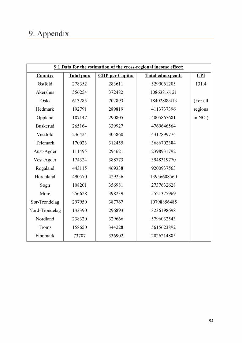
94
9. Appendix
9.1 Data for the estimation of the cross-regional income effect:
County:
Østfold
Akershus
Oslo
Hedmark
Oppland
Buskerud
Vestfold
Telemark
Aust-Agder
Vest-Agder
Rogaland
Hordaland
Sogn
Møre
Sør-Trøndelag
Nord-Trøndelag
Nordland
Troms
Finnmark
Total pop:
278352
556254
613285
192791
187147
265164
236424
170023
111495
174324
443115
490570
108201
256628
297950
133390
238320
158650
73787
GDP per Capita:
283611
372482
702893
289819
290805
339927
305860
312455
294621
388773
469338
429256
356981
398239
387767
296893
329666
344228
336902
Total eduexpend:
5299061205
10863816121
18402889413
4113737396
4005867681
4769646564
4317899774
3686702384
2398931792
3948319770
9200937563
13956608560
2737632628
5521375969
10798856485
3236198698
5796032543
5615623892
2026214885
CPI
131.4
(For all
regions
in NO.)

95
9.2 Data for the estimation of the cross-regional income effect:
County:
Østfold
Akershus
Oslo
Hedmark
Oppland
Buskerud
Vestfold
Telemark
Aust-Agder
Vest-Agder
Rogaland
Hordaland
Sogn
Møre
STrøndelag
NTrøndelag
Nordland
Troms
Finnmark
EnrollP:
34589
76145
59631
25183
22242
32612
20372
14364
22992
59624
62341
14406
33051
35989
17582
29636
29636
19416
9403
EnrollS:
11015
22879
16741
7493
7337
10033
9622
6825
4586
7421
18515
19491
4813
10403
11270
5788
10161
6652
3181
EnrollH:
13916
27945
31509
9917
9738
13170
12153
9088
6007
10126
24400
27450
6121
13752
17529
7329
13126
8929
4132
ExpendP:
3131169225
6367016465
5420100114
2486846433
2330983842
3018110152
2605553200
2107931584
1424923164
2218222176
5472827336
5945835216
1610158620
3263422689
3427160492
1826189594
3212720216
2059338624
1143583457
ExpendS:
1644891980
3492799656
2388656103
1114890963
1078883839
1355327871
1217346574
971770800
675508628
967624190
2435944490
2674594002
813474008
1557953280
1542209340
973009104
1719312327
1107285268
577631428
ExpendH:
523000000
1004000000
10594133196
512000000
596000000
396208541
495000000
607000000
298500000
762473404
1292165737
5336179342
314000000
700000000
5829486653
437000000
864000000
2449000000
305000000
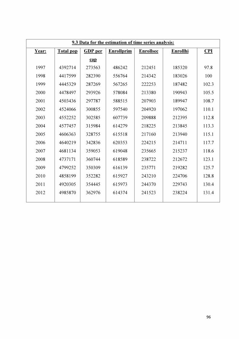
96
9.3 Data for the estimation of time series analysis:
Year:
1997
1998
1999
2000
2001
2002
2003
2004
2005
2006
2007
2008
2009
2010
2011
2012
Total pop
4392714
4417599
4445329
4478497
4503436
4524066
4552252
4577457
4606363
4640219
4681134
4737171
4799252
4858199
4920305
4985870
GDP per
cap
273563
282390
287269
293926
297787
300855
302585
315984
328755
342836
359053
360744
350309
352282
354445
362976
Enrollprim
486242
556764
567265
578084
588515
597540
607739
614279
615518
620353
619048
618589
616139
615927
615973
614374
Enrollsec
212451
214342
222253
213380
207903
204920
209888
218225
217160
224215
235665
238722
235771
243210
244370
241523
Enrollhi
185320
183026
187482
190943
189947
197062
212395
213845
213940
214711
215237
212672
219282
224706
229743
238224
CPI
97.8
100
102.3
105.5
108.7
110.1
112.8
113.3
115.1
117.7
118.6
123.1
125.7
128.8
130.4
131.4

97
9.4 Data for the estimation of time series analysis:
Year:
1997
1998
1999
2000
2001
2002
2003
2004
2005
2006
2007
2008
2009
2010
2011
2012
Eduspendprim
24372000000
27052000000
27504000000
31591000000
34536000000
38017000000
40875000000
42249000000
44146000000
46576000000
49269000000
52530000000
56364000000
59393000000
60658000000
59072000000
Eduspendsec
11997000000
12724000000
12727000000
13418000000
14876000000
15603000000
17317000000
17510000000
18374000000
19405000000
20359000000
22388000000
24013000000
24651000000
25341000000
28309000000
Eduspendhi
15121000000
16797000000
17690000000
18385000000
19544000000
21436000000
23133000000
24714000000
25392000000
26827000000
28425000000
30236000000
32408000000
32778000000
34134000000
30904000000
Eduspendtot
51490000000
56573000000
57921000000
63394000000
68956000000
75056000000
81325000000
84473000000
87912000000
92808000000
98053000000
105154000000
112785000000
116822000000
120133000000
118285000000
Aggprivate
Spend*
2999158481
3344061706
3728628803
4157421115
4635524543
5168609865
5763000000
6763000000
7517000000
8337000000
9662000000
11086000000
11996000000
13701000000
14310000000
15955650000
* Private education spending in time series have been estimated for all but 5 years. Expenditure data are
available for 2005-2009, and on the background of these numbers, an estimate of the average growth in
the available expenditures have been computed for all numbers post 2009. Hence, this average rate is
used to deflate all numbers pre-2005, assuming that the expenditures for private numbers are growing
from the first period and until the last. The analysis framework and the discussion part argues around
this way of estimating when data shows an almost constant demand for private education relative to the
total education spending in Norway.
** All numbers from the regression analysis in chapter 6 have been estimated by the use of table 9.1-9.4
through the statistics software IBM SPSS v2.1

98
9.5 Breusch-Pagan Test of Heteroscedasticity:
Model: BP-statistic: p-value:
Two-step Analysis:
IncomeP
IncomeS
IncomeH
PriceP
PriceS
Time Series Analysis, high edu:
All variables
PPriv omitted
PGov omitted
All price omitted
Aggregate Demand:
Two-step Income
Two-step Price
Time Series Aggregate
Two-Component Aggregate:
Government:
Two-step Gov Income
Two-step Gov Price
Time Series Gov
Private:
Two-step Priv Income
Two-step Priv Price
Time Series Priv
1.026
0.536
0.094
0.571
0.003
4.664
1.814
3.938
0.416
0.081
1.905
2.006
0.020
1.998
2.008
0.043
1.403
0.971
0.31
0.46
0.76
0.45
0.98
0.32
0.61
0.27
0.81
0.78
0.17
0.37
0.89
0.16
0.37
0.83
0.24
0.62
^ None of the values in this BP test was found significant, therefore all models exhibit homoscedasticity.
~ The BP test was conducted by the use of the regression software R. The test was obtained through the package
“lmtest”, using the function “bptest” to test for heteroscedasticity.