emissions, physicochemical characteristics and exposure …epubs.surrey.ac.uk/810771/1/farhad...
TRANSCRIPT

Emissions, physicochemical characteristics and exposure to
coarse, fine and ultrafine particles from building activities
Department of Civil and Environmental Engineering
Faculty of Engineering and Physical Sciences
University of Surrey
Guildford, Surrey, UK
A thesis submitted for the fulfillment of
Doctor of Philosophy
by
Farhad Azarmi
Copyright © Farhad Azarmi, 2016

Statement of Originality
The work presented in this dissertation was carried out by the author at the Department of
Civil and Environmental Engineering, University of Surrey (UK), under the supervision of
my principal supervisor, Dr. Prashant Kumar, and co-supervisor, Dr. Mike Mulheron. This
thesis is my own work and contains nothing which is the outcome of my work performed
in collaboration with others. Any published (or unpublished) ideas and/or techniques from
the work of others are fully acknowledged in accordance with the standard referencing
practices. In addition, no part of this thesis has already been, or is being concurrently
submitted for any other degree, diploma or qualification.
This dissertation contains approximately 54,516 words, 48 figures and 24 tables.
Farhad Azarmi
University of Surrey
Friday, 11th of March, 2016

Acknowledgements
Firstly, I would like to express my sincere thanks and appreciation to my principal
supervisor, Dr. Prashant Kumar for all his excellent supervision, constant support and
kindness over the duration of my PhD. My discussions with Dr. Kumar and his insights
always helped me to get back on the right direction. Dr. Kumar cared so much about my
work and responded to all my queries and questions so promptly. His patient guidance and
encouragement has given to me the confidence and assurance to carry on this research
study. I also thank my co-supervisor, Dr. Mike Mulheron, for his valuable help and advice
throughout the research duration.
I am very grateful to the Department of Civil and Environmental Engineering, University
of Surrey for providing PhD funding support and cara for this work. I am thankful to Prof.
Stephen Baker and Stuart Robinson for permitting the access of the demolition site. Thanks
also to Prof. Vincent Emery, Dr. Norma Denny, Dr. Gary Fuller, Chris Burt, Alan Newland,
Russell Bridges-Smith, Stephen Knight, Daniel Marsh, Shoaib Shafi and Nigel Mobb for
all their helps during my PhD programme. Furthermore, I would like to thank Anju Goel,
Omid Eshaghi, Hossein Jahangiri, Hesam Mehrabi, Zhenchun Yang, Abdullah Al-
Dabbous, Dr. Siavash Adhami and Dr. Sanjay Mukherjee and all the faculty staff for their
great supports and helps throughout my research study as a PhD student.
Last but not least, I would like to present my heartfelt thanks to my family for all their
precious love, support and encouragement through my years of study.

Publications
The work described in this thesis appeared in the following published articles and
presentations:
Journal Articles
Azarmi, F., Kumar, P., Mulheron, M., 2014. The exposure to coarse, fine and ultrafine
particle emissions from concrete mixing, drilling and cutting activities. Journal of
Hazardous Materials 279, 268-279.
Azarmi, F., Kumar, P., Mulheron, M., Colaux, J.L., Jeynes, C., Adhami, S., Watts, J.F.,
2015. Physicochemical characteristics and occupational exposure to coarse, fine
and ultrafine particles during building refurbishment activities. Journal of
Nanoparticle Research 17, 343, doi: 10.1007/s11051-015-3141-z.
Azarmi, F., Kumar, P., Marsh, D., Fuller, G.W., 2015. Assessment of long-term impacts of
PM10 and PM2.5 particles from construction works on surrounding areas.
Environmental Science: Processes & Impacts 18, 208-221.
Azarmi, F., Kumar, P., 2016. Ambient exposure to coarse and fine particle emissions from
building demolition. Atmospheric Environment 137, 62-79.
Conference Articles and Presentations
Azarmi, F., Kumar, P., Mulheron, M., 2014. Coarse and fine particulate emissions from
drilling activity. 4th Postgraduate research Conference, 3rd-4th February, Surrey
University Conference, United Kingdom.

Azarmi, F., Kumar, P., Mulheron, M., 2015. Occupational exposure to coarse, fine and
ultrafine particle emissions from building refurbishment activities. International
Festival of Public Health, University of Manchester, United Kingdom, July 2015.
Azarmi, F., Kumar, P., 2015. Assessment of impact of coarse and fine particles from
building demolition works on surrounding areas. 10th International Conference on
Air Quality-Science and Application, 14th-18th March, Milan, Italy (accepted).
Book chapters
Kumar, P., Azarmi, F., Mulheron, M., 2012. Enlightening and noxious shades of
nanotechnology application in concrete. In: Nanotechnology: Volume 9 Civil /
Construction Engineering. (Studium Press LLC, USA; Govil, J.N. Eds.). ISBN: 1-
62699-009-3). pp. 255-287.
News stories
DIY can be dangerous – but it’s the invisible dust that may harm you the most, The
Conversation, 20 August 2015
How the dust from DIY jobs can give you heart disease or cancer: Call for health and safety
regulations to be updated to protect builders and amateur enthusiasts, Mail Online,
20 August 2015.
Warning to DIY enthusiasts and construction workers as dangerous dust emissions, Science
Newsline, 19 August 2015.
DIY Techniques are found to be less productive, Nature World News, 27 August 2015.
Abstract
Building works include construction and demolition activities, which are common in cities
across the world. Building-related activities contribute a considerable amount of the
construction and demolition waste material worldwide. These activities have the potential
to produce particulate matter (PM), including PM10 (≤10 μm), PM2.5 (≤2.5 μm) and PM1
(≤1 μm), and airborne ultrafine particles (≤0.1 μm). Recent studies have indicated that the
rate of building works undertaken each year is growing exponentially, to meet new urban
design guidelines and respond to demand from the adoption of new building technologies,
which highlights the importance of measuring the amounts of particle emissions from these
sources. The principles of sustainable urban development are well established, but the
extent of pollution due to construction and demolition activities is still unknown. Through
laboratory and field studies, this thesis aims to comprehensively investigate the release of
coarse (referred to as PM2.5–10 fraction), fine (PM2.5) and ultrafine particles from various
building works, assess their physicochemical properties, and estimate the associated
occupational exposure risk from them to on-site workers and individuals in the close
vicinity.
Experiments for this thesis were carried out to measure PM and airborne ultrafine particles
in the size range of (0.005–10 µm) using a fast response differential mobility spectrometer
(DMS50), a tapered element oscillating micro balance (TEOM 1400), a GRIMM particle
spectrometer (1.107 E) and OSIRIS (2315). Measurements were made in various locations:
a controlled laboratory environment (i.e. concrete mixing, drilling, cutting), indoor field
sites (i.e. building refurbishment) and at outdoor field sites (i.e. construction and
demolition). Moreover, dust samples were collected simultaneously for physiochemical
analyses (e.g. SEM, EDS, XPS and IBA). Several important findings were then
extrapolated during the analysis. These findings indicated that ultrafine particles dominated
(74-97%) the total particle number concentrations (PNCs) while the coarse particles (PM2.5-
10) contributed to the majority of the total particle mass concentrations (PMCs), during the
laboratory, indoor and outdoor field experiments. The highest proportion of PNCs and
PMCs was found during the concrete cutting, drilling and wall chasing activities. In
addition, the highest proportion of PMCs was observed in the excavator cabin during a
building demolition at an outdoor field measurement site. Moreover, combining the results
of SEM, EDS, XPS and IBA analysis suggested the dominance of elements such as Si, Al
and S in the collected samples. The data were also used to assess the horizontal decay of
the PMC through a modified box model to determine the emission factors and the
occupational exposure to on-site workers and nearby individuals. The results confirmed
that building-related works produce significant levels of coarse, fine and ultrafine particles,
and that there is a need to limit particle emissions and reduce the occupational exposure of
individuals by enforcing effective engineering controls. These findings could also be useful
for the building industry to develop mitigation strategies to limit exposure to particulate
matter during building works, particularly for ultrafine particles, which are currently non-
existent.

i
Table of Contents
Chapter 1. Introduction ............................................................................................... 1
1.1 Motivation ............................................................................................................ 1
1.2 Research objectives .............................................................................................. 3
1.3 Research approach ................................................................................................ 4
1.3.1 Simulated laboratory investigations .............................................................. 4
1.3.2 Release of particles from indoor activities of building refurbishment ......... 4
1.3.3 Assessment of PM10 and PM2.5 particles from outdoor construction activities
5
1.3.4 Exposure to particles from outdoor building demolition activities .............. 6
1.4 Thesis outline ....................................................................................................... 7
Chapter 2. Background concepts and literature review ............................................ 10
2.1 General overview of PM and ultrafine particles ................................................ 10
2.2 Particle size distribution, modes and fractions ................................................... 12
2.3 Particle mass and number concentrations .......................................................... 15
2.4 Sources of PM and ultrafine particle emissions in the urban environment ........ 16
2.5 Particle emissions from building activities ........................................................ 19
2.5.1 Importance of particle emissions from building activities .......................... 19
2.5.2 Building-related sources of PM and ultrafine particle emissions ............... 21
ii
2.6 Physiochemical characteristics of particles ........................................................ 27
2.6.1 Scanning electron microscopy (SEM) ........................................................ 28
2.6.2 Energy-dispersive X-ray spectroscopy (EDS) ............................................ 29
2.6.3 Ion Beam Analysis (IBA) ........................................................................... 30
2.6.4 X-ray Photoelectron Spectroscopy (XPS) .................................................. 31
2.7 Environmental and health impacts of exposure to atmospheric particles .......... 32
2.7.1 Health effects .............................................................................................. 33
2.7.2 Visibility and climate change ...................................................................... 35
2.8 Regulations, guidance and limits for PM and ultrafine particles ....................... 37
2.9 Chapter summary ............................................................................................... 40
Chapter 3. Materials and methods ............................................................................ 41
3.1 Introduction ........................................................................................................ 41
3.2 Instrumentation ................................................................................................... 42
3.2.1 GRIMM (1.107 E) ...................................................................................... 42
3.2.2 DMS50 ........................................................................................................ 43
3.2.3 OSIRIS (2315) ............................................................................................ 45
3.2.4 TEOM (1400) .............................................................................................. 45
3.2.5 Kestrel 4500 weather station ....................................................................... 46
3.2.6 GPS ............................................................................................................. 46
3.3 Physicochemical analysis ................................................................................... 47

iii
3.3.1 SEM and EDS analysis ............................................................................... 47
3.3.2 XPS analysis ............................................................................................... 47
3.3.3 IBA analysis ................................................................................................ 48
3.4 Emission factors ................................................................................................. 49
3.4.1 Simulated laboratory investigations ............................................................ 49
3.4.2 Building demolition .................................................................................... 50
3.5 Estimation of exposure doses for health risk analysis........................................ 54
3.5.1 Exposure doses of ultrafine particles .......................................................... 54
3.5.2 Exposure doses of PM10, PM2.5 and PM1 .................................................... 56
3.6 Chapter summary ............................................................................................... 58
Chapter 4. Simulated laboratory investigations ........................................................ 59
4.1 Introduction ........................................................................................................ 59
4.2 Methodology ...................................................................................................... 61
4.2.1 Experimental setup ...................................................................................... 61
4.3 Results and discussion ........................................................................................ 65
4.3.1 Particle size distributions ............................................................................ 65
4.3.2 Particle number concentrations ................................................................... 67
4.3.3 Particle mass concentrations ....................................................................... 71
4.3.4 Emission factors .......................................................................................... 75
4.3.5 Exposure assessment ................................................................................... 78

iv
4.4 Chapter summary and conclusions ..................................................................... 80
Chapter 5. Indoor building refurbishment activities ................................................. 83
5.1 Introduction ........................................................................................................ 83
5.2 Materials and methods ....................................................................................... 86
5.2.1 Site description and sampling setup ............................................................ 86
5.2.2 Collection of PM mass on PTFE filters for SEM, IBA and XPS analysis . 89
5.3 Results and discussion ........................................................................................ 89
5.3.1 Number and size distribution of particles ................................................... 90
5.3.2 Particle number concentrations ................................................................... 94
5.3.3 Particle mass concentrations ....................................................................... 97
5.4 Morphology assessment and chemical characterization .................................. 102
5.4.1 XPS and SEM analysis ............................................................................. 102
5.4.2 IBA analysis .............................................................................................. 105
5.5 Exposure assessment ........................................................................................ 106
5.6 Chapter summary and conclusions ................................................................... 108
Chapter 6. Outdoor construction activities ............................................................. 111
6.1 Introduction ...................................................................................................... 111
6.2 Materials and methods ..................................................................................... 113
6.2.1 Description of the sites and sampling set ups ........................................... 113
6.3 Results and discussion ...................................................................................... 118

v
6.3.1 Bivariate concentration polar plots ........................................................... 118
6.3.2 Assessment of paired sites for examining differences in PM concentrations
122
6.3.3 k-means clusters analysis .......................................................................... 124
6.3.4 Particle mass concentrations during working and non-working hours ..... 128
6.3.5 Decay profiles of PM10 and PM2.5 ............................................................ 135
6.4 Chapter summary and conclusions ................................................................... 137
Chapter 7. Outdoor building demolition activities.................................................. 140
7.1 Introduction ...................................................................................................... 140
7.2 Materials and methods ..................................................................................... 143
7.2.1 Sampling set up and site description ......................................................... 143
7.2.2 Collection of PM mass on PTFE filters for SEM and EDS analysis ........ 147
7.3 Results and discussion ...................................................................................... 148
7.3.1 PMCs downwind of the demolition site .................................................... 148
7.3.2 Spatial variations of PM during mobile measurements ............................ 151
7.3.3 Concentrations inside the excavator cabin and temporary on-site office . 156
7.3.4 PM decay profiles ..................................................................................... 159
7.3.5 The PMEFs for building demolition ......................................................... 161
7.3.6 Morphology and chemical characterisation .............................................. 162
7.3.7 Exposure to demolition workers and engineers ........................................ 166

vi
7.4 Chapter summary and conclusions ................................................................... 169
Chapter 8. Summary, conclusions and future work ................................................ 173
8.1 Summary .......................................................................................................... 173
8.1.1 Simulated laboratory investigations .......................................................... 174
8.1.2 Release of particles from indoor activities of building refurbishment ..... 175
8.1.3 Assessment of PM10 and PM2.5 particles from outdoor construction activities
176
8.1.4 Exposure to particles from outdoor building demolition activities .......... 177
8.2 Conclusions ...................................................................................................... 178
8.3 Recommendations for future research .............................................................. 181
References ....................................................................................................................... 184
Appendix A ............................................................................................................. 213
Appendix B ............................................................................................................. 218
Appendix C ............................................................................................................. 230
Appendix D ............................................................................................................. 238
vii
List of Figures
Figure 1.1: Report outline presenting the work breakdown structure for the main chapters.
............................................................................................................................................. 7
Figure 2.1: The aerodynamic equivalent diameter of an irregular and a spherical shaped
particle (Hinds, 1999) ....................................................................................................... 11
Figure 2.2: Typical particle size distribution by number and mass weightings showing
different size modes (Kittelson, 1998) .............................................................................. 14
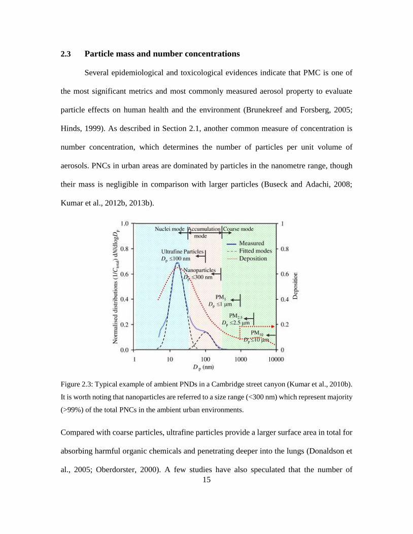
Figure 2.3: Typical example of ambient PNDs in a Cambridge street canyon (Kumar et al.,
2010b). It is worth noting that nanoparticles are referred to a size range (<300 nm) which
represent majority (>99%) of the total PNCs in the ambient urban environments ........... 15
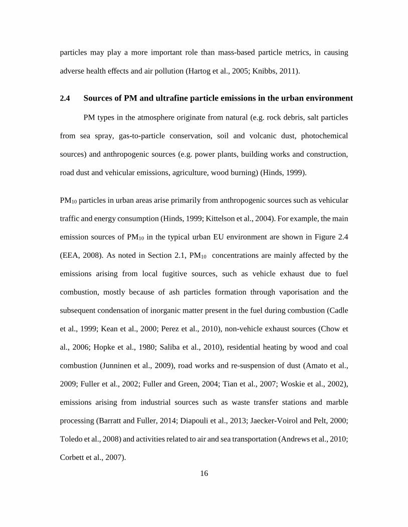
Figure 2.4: Emission sources of PM10 (Gg per year) in EU urban locations; adapted from
EEA (2008). Others sources represented in this figure refer to agriculture, construction and
secondary sources ............................................................................................................. 17
Figure 2.5: Emission source of ambient PM2.5 (Gg per year) in EU urban locations; adapted
from EEA (2008). Other sources in this figure refer to agriculture, construction and
secondary sources ............................................................................................................. 18
Figure 2.6: Particle size and specific surface area of concrete materials; taken from Kumar
et al. (2012a) ..................................................................................................................... 24
Figure 2.7: Relaxation of the ionized atom of Auger electron and X-ray electron emission
(Watts, 1990) ..................................................................................................................... 32
Figure 3.1: Schematic diagram of the box model, showing various dimensions and
parameters; fx and fz refer to the particulate mass flow rate entering and leaving the box in
the x and z directions, respectively. Ux and Uz refer to wind velocities in the x and z
viii
directions; L and W refer to length and width of the box, respectively, and Hm refers to
maximum mixing height ................................................................................................... 51
Figure 3.2: Finding mass median diameter (MMD) of coarse and fine particles using
cumulative particle mass concentrations measured during each activity. DF refers to
deposition fraction which has been estimated using MMD in Eq. (3.11). ........................ 57
Figure 4.1: Schematic of the experiment showing instrumentation used and distances; Lc,
Ld and Lm represents the length between the DMS50 and the sampling points from cutter,
drilling and mixer, respectively. Length of all these sampling tubes is 1 m. .................... 64
Figure 4.2: PNDs for the (a) mixing with GGBS and (b) mixing PFA, (c) drilling, and (d)
cutting ............................................................................................................................... 66
Figure 4.3: Temporal evolution of PNC and their contour plots during (a) mixing with
GGBS, and (b) mixing with PFA ...................................................................................... 68
Figure 4.4: Temporal evolution of PNC and their contour plots during (a) drilling, and (b)
cutting activities ................................................................................................................ 70
Figure 4.5: Mass concentration against time for (a) mixing with GGBS, (b) mixing with
PFA, (c) drilling, and (d) cutting activities ....................................................................... 72
Figure 4.6: Particle number concentration based EFs for all the four activities. Please note
that these are net EFs estimated using the net sum of PNCs (i.e. total during the activity
period minus the background PNCs during pre-activity period) ...................................... 77
Figure 4.7: Particle mass concentration based EFs for all the four activities. Please note
that these are net EFs estimated using the net sum of PMCs (i.e. total during the activity
period minus the background PMCs during pre-activity period) ..................................... 78
ix
Figure 4.8: Respiratory tract deposition dose rate (# min−1) calculated using (i) size-
dependent DFs and average size-resolved PNCs, and (ii) a constant DF and the average
PNC for each activity ........................................................................................................ 79
Figure 5.1: Schematic diagram of the experimental set-up, showing instrumentation used
and sampling locations ...................................................................................................... 87
Figure 5.2: Number of typical activities involved in refurbishment works including (a)
drilling of wood, (b) drilling of concrete slab, (c) cutting, (d) hammering, (e) sanding and
(f) ceiling drilling activities .............................................................................................. 88
Figure 5.3: Average PNDs during the background, activity and non-activity periods ..... 91
Figure 5.4: Average PNDs and proportion of PNCs in various size ranges for the individual
activities. Other activities refer to painting, oiling, carrying metal bars to the site and
moving demolished debris ................................................................................................ 92
Figure 5.5: Average PNCs during the background, activity and non-activity periods ..... 94
Figure 5.6: The Average PNCs on a daily basis during the background, activity and non-
activity periods. The inner and outer circles represent fractions of PNCs in various size
ranges during the activity and non-activity periods, respectively ..................................... 96
Figure 5.7: The concentrations of PM10, PM2.5 and PM1 during the background, activity
and non-activity periods .................................................................................................... 97
Figure 5.8: The average concentrations of PM10, PM2.5 and PM1 during the background,
activity and non-activity period for each day of activity .................................................. 98
Figure 5.9: The concentrations of PM10, PM2.5 and PM1 during the background and activity
period (details of each activity time period is listed in Table B1) .................................. 100

x
Figure 5.10: SEM images of (a) blank filter at ×500, (b) background measurements at
×8000, (c) sample 1 at ×1000, (d) sample 1 at ×8000, (e) sample 2 at ×600, (f) sample 2 at
×8000, (g) sample 5 at ×8000, and (h) sample 5 at ×16000 ........................................... 104
Figure 5.11: Respiratory tract deposition dose rate (# min−1) calculated using (i) a constant
DF and the average PNC during each activity and (ii) size-dependent DFs and average size-
resolved PNCs ................................................................................................................. 107
Figure 6.1: Schematic map of the experimental set-up, showing monitoring stations (MS)
and construction sites: (a) one (CS1), (b) two (CS2) and (c) three (CS3). Please note that the
figure is not to scale and distances are presented in Table 6.1 ....................................... 116
Figure 6.2: Polar plots for PM10 at the (a) CS1, (b) CS2 and (c) CS3; hourly average values
during 24-h measurements were used for all pollutants. These plots present as smoothed
surfaces how concentrations vary depending on the local wind speed and wind direction.
......................................................................................................................................... 120
Figure 6.3: Polar plots for PM2.5 (hourly average values during 24-h measurements were
used for all pollutants) at the CS1. These plots present as smoothed surfaces how
concentrations vary depending on the local wind speed and wind direction .................. 121
Figure 6.4: The polar plots for the paired monitoring stations across each construction site,
for ΔPM10 and ΔPM2.5 (a) at the CS1 and (b) for ΔPM10 at the CS2, respectively .......... 123
Figure 6.5: Clusters identified at CS1 and CS2 sites for PM10 concentrations for 8 clusters.
The shading shows the 95% confidence intervals in the mean. The data have been
normalised in each case by dividing by the mean ........................................................... 126

xi
Figure 6.6: Clusters identified at CS1 for PM2.5 concentrations for 8 clusters. The shading
shows the 95% confidence intervals in the mean. The data have been normalised in each
case by dividing by the mean .......................................................................................... 127
Figure 6.7: The annual average concentrations of PM10 (17 monitoring stations) during
2002-2013 period at the (a) CS1, (b) CS2, and (c) CS3 ................................................... 128
Figure 6.8: Numbers of exceedences over the EU limit value at the individual monitoring
stations ............................................................................................................................ 133
Figure 6.9: ΔPM10 and ΔPM2.5 concentration decay at CS1 and CS2 versus distance in the
direction of wind blowing from construction sites, showing (a) logarithmic, and (b)
exponential best fit functions .......................................................................................... 136
Figure 7.1: Sample of demolition works at the demolition site ...................................... 144
Figure 7.2: Schematic map of the experimental set-up, showing (a, b) monitoring stations
around the demolition site (DS) during (c) fixed site measurements at day 2, and (d) day 3.
Route of mobile measurements around the DS during (e) day 4, and (f) day 5. SP and EP
refer to the start and end points, respectively, while the arrows represent the path of mobile
measurements .................................................................................................................. 146
Figure 7.3: Wind roses diagrams depict the hourly frequency distribution of the wind speed
and direction during the fixed site measurement on day 2 (a) and day 3 (b), as well as during
the mobile measurements on day 4 (c) and day 5 (d), for sequential distances at day 6 (e)
and day 7 (f) .................................................................................................................... 147
Figure 7.4: (a) The average concentrations of PM10, PM2.5 and PM1 with average of
prevailing wind direction, during all days of fixed site measurements. The inner and outer
circles represent fractions of PMCs in various size range .............................................. 150
xii
Figure 7.5: The average concentrations of PM10, PM2.5 and PM1, at (a) route A and (b) route
B, during all days of mobile measurements. The inner and outer circles represent fractions
of PMCs in various size ranges during the background and activity periods. Please note
that SP and EP refer to the start and end points, respectively ......................................... 153
Figure 7.6: The spatially averaged concentrations of PM10, PM2.5 and PM1 during mobile
measurements at (a) route A and (b) route B. The words Avg, DW and UW in the figure
represent average, downwind and upwind, respectively. A number of parallel points at each
route were due to the sensitivity of GPS device, which varied within ±3.5 m at the same
route ................................................................................................................................ 155
Figure 7.7: The concentrations of PM10, PM2.5 and PM1, at (a) the excavator cabin and (b)
temporary on-site office for site engineers and managers during the background and
working periods, respectively ......................................................................................... 157
Figure 7.8: (a) Horizontal decay profiles of ΔPM10, (b) ΔPM2.5 and (c) ΔPM1 at the
demolition site during the sequential measurements; x and y expresses distance from the
demolition site and ΔPM values, respectively ................................................................ 160
Figure 7.9: SEM images of the surface morphology of the particles collected on blank filter,
background measurements, sample 3, sample 4 and sample 5 at ×50, ×1000 and ×8000
resolution. ........................................................................................................................ 165
Figure 7.10: Factor of increased exposure (FIE) representing a ratio of respiratory
deposition doses during the activities over the background level in coarse and fine particles
range during each activity ............................................................................................... 167

xiii
List of Tables
Table 2.1: Summary of past studies showing measured particle number and mass
concentrations from various building activities ................................................................ 21
Table 2.2: Summary of physicochemical analysis of particles collected during number of
building-related activities. ................................................................................................. 28
Table 2.3: Summary of ambient air quality limits and standards; (Directive, 2008; EPA,
2011; WHO, 2006; CPCB, 2010; Kumar, 2009). Please note that N.S. refers to not specified
........................................................................................................................................... 39
Table 3.1: Summary of the instruments used for measuring PM10, PM2.5, PM1 and ultrafine
particles during experiments ............................................................................................. 42
Table 3.2: Measuring capabilities of DMS50 (Kumar et al., 2010a) and GRIMM (Cheng,
2008) ................................................................................................................................. 44
Table 4.1: Summary of sampling data during concrete mixing, drilling and cutting activities
........................................................................................................................................... 63
Table 4.2: Average concentration, geometrical mean diameter and fractions for particles
number during mixing, drilling and cutting activities. ..................................................... 67
Table 4.3: The concentrations of PM10, PM2.5 and PM1 during the activity period. STD and
percentage fraction (PF) represent standard deviation and particles fraction of mixing with
GGBS, PFA, drilling and cutting, respectively. ................................................................ 75
Table 5.1: Summary of samples collected on PTFE filters during the refurbishment activity.
........................................................................................................................................... 89
Table 5.2: Average values of PNCs during the background, activity and non-activity
periods on different days ................................................................................................... 96
xiv
Table 5.3: The concentrations of PM10, PM2.5 and PM1 during the background, activity and
non-activity periods on different days. ............................................................................. 98
Table 5.4: The elemental composition of the all the filters (quantitative XPS analyses).
......................................................................................................................................... 103
Table 6.1: Description of monitoring stations around the construction sites. Monitoring
stations S1-S9, S10-S15, and S16-S17 below are around the CS1, CS2 and CS3, respectively
......................................................................................................................................... 117
Table 6.2: The annual average concentrations of PM10 including the working and non-
working periods at the CS1; ± refers to standard deviation and “–” to the unavailability of
data .................................................................................................................................. 130
Table 6.3: The annual average concentrations of PM2.5 including the working and non-
working periods at the CS1; ± refers to standard deviation and “–” to the unavailability of
data .................................................................................................................................. 130
Table 6.4: The annual average concentrations of PM10 including the working and non-
working periods; ± refers to standard deviation and “–” to the unavailability of data. .. 131
Table 6.5: The average concentrations of PM10 including the working and non-working
periods at the CS3; ± refers to standard deviation ........................................................... 131
Table 6.6: Summary of EU air quality limit values against AQS objectives (Directive,
1999; Directive, 2008; Fuller and Green, 2004) ............................................................. 132
Table 6.7: Number of exceeded days from the EU standard limit and UK government
objective (AQS). Please note that the excedances presented in the parenthesis against each
exceedance number represent the exceedances belonging to the 24 hours. ................... 134
Table 7.1: Description of sampling duration and monitoring sites ................................. 145

xv
Table 7.2: Summary of samples collected on PTFE filters during the demolition activity.
......................................................................................................................................... 148
Table 7.3: PM10, PM2.5 and PM1 concentrations (µg m-3) during mobile measurements at
routes A and B ................................................................................................................ 156
Table 7.4: The elemental composition of the all the filters (quantitative EDS analyses).
......................................................................................................................................... 164
Table 7.5: The RDD rates of coarse and fine particles ................................................... 168

xvi
Glossary
List of Acronyms
AQS Air Quality Strategy
AVG Average
COSHH Control of Substances Hazardous to Health
CS Construction site
DF Deposition fraction
DS Demolition site
EBS Elastic backscattering spectrometry
EDS Energy dispersive x-ray spectroscopy
EF Emission factor
EMEP European Monitoring and Evaluation Programme
EEA European Environment Agency
ENP Engineered nanoparticles
EPA Environmental Protection Agency
EU European Union
FIB Focused Ion Beam
GGBS Ground Granulated Blastfurnace Slag
GPS Global Positioning System

xvii
HEPA High efficiency particulate air filter
HSE Health and Safety Executive
IBA Ion Beam Analysis
ICRP International Commission on Radiological Protection
MMD Mass median diameter
MLD Minimum level of detection
MS Monitoring station
NAEI National Atmospheric Emission Inventory
NIST National Institute of Standards and Technology
PFA Pulverised Fuel Ash
PM Particulate matter
PM10 Particles with diameter ≤10 µm
PM2.5 Particles with diameter ≤2.5 µm
PM1 Particles with diameter ≤1 µm
PMC Particle mass concentration
PMEF Particle mass emission factor
PND Particle number distribution
PNC Particle number concentration
PIXE Particle Induced X-ray Emission

xviii
PSL Polystyrene Latex Sphere
PTFE Polytetrafluoroethylene
PVC Polyvinyl chloride
RDD Respiratory deposited doses
SEM Scanning electron microscope
STD Standard deviation
UFP Ultrafine particle
UK United Kingdom
USA United States of America
VT Tidal volume
WD Wind direction
WEL Work Exposure Limit
WHO World health organization
WS Wind speed
XPS X-ray Photoelectron Spectroscopy
1
Chapter 1. Introduction
This chapter provides an overview of the research in the context of emissions,
physicochemical characteristics and exposure to coarse, fine and ultrafine particles from
building activities. The chapter starts with the background and motivation for the study;
this is followed by a summary of research objectives and approaches, and a conclusion
briefly outlining the structure of the thesis.
1.1 Motivation
Exposure to particulate matter (PM), including PM10 (≤10 µm), PM2.5 (≤2.5 µm)
and PM1 (≤1 µm), and ultrafine particles (≤0.1 µm), is of great concern to the air quality
management community due to these particles’ potentially adverse impacts on human
health and the environment (Chow et al., 2006; Kumar et al., 2010a). There is substantial
epidemiological and toxicological evidence to suggest that it is important to evaluate the
influence of both particle number concentrations (PNCs) and particle mass concentrations
(PMCs) on human health (Brunekreef and Forsberg, 2005; Heal et al., 2012). Particle size
is important, as smaller particles can penetrate deeper into the respiratory system,
increasing the potential to adversely affect human health (Hoet et al., 2004). Some studies
have speculated that when considering exposure to ultrafine particles, PNC is a more
important exposure metric than the particle mass-based metric (Hartog et al., 2005).

2
Typically, ultrafine particles are represented by PNCs, whilst the PM10, PM2.5 and PM1
particles are represented based on PMCs (Kumar and Morawska, 2014).
Within urban environments there are a number of sources of ultrafine particles and PM.
Vehicle emissions and road works are well-established sources of PNCs and PMCs (Amato
et al., 2009; Kumar et al., 2013b; Pey et al., 2009). Previous studies have drawn attention
to other sources of PM10, PM2.5, PM1 and ultrafine particles, such as fossil fuel burning,
mineral industries, mineral dust, and secondary aerosols (Querol et al., 2004; Yatkin and
Bayram, 2008). There are many negative impacts on human health and the environment
through exposure to PM and ultrafine particles , which may lead to higher rates of mortality
around the world (Jacobson, 2005; Kumar et al., 2011a; Stjern et al., 2011).
Consequently, the continuous development of civil and urban infrastructures has led to the
imposition of more stringent regulations on the use of construction materials, and on the
way work is undertaken. Building-related activities have the potential to generate coarse
(hereafter referred to PM2.5–10 fraction), fine (PM2.5) and ultrafine particles due to the
increase in the world population and the growing need for construction and demolition
works. However, the exact quantities of PM and ultrafine particles produced, and the
occupational exposure level of operatives, are poorly understood. This is slowly changing as
we become concerned with climate change and health issues, which highlighting a need to
protect the environment, improve quality of life and sustain the liveable conditions in urban
areas.

3
Whilst research studies have been undertaken to investigate the effects of PM and ultrafine
particles on the environment and health, there is still very little and limited legal regulation,
and a lack of guidelines for restricting public exposure to airborne particles – especially for
ultrafine particles – within the urban environment and at construction and demolition sites.
Setting up health and safety regulatory bodies as a basis for establishing such guidelines is
very important, as there is a clear need to investigate the release of airborne particles.
Therefore, the focus of this thesis remains mainly on building activities where very little is
currently known.
1.2 Research objectives
The aim of this work is to understand how PM and ultrafine particles are emitted
from various indoor and outdoor building sources and assess the physicochemical
characteristics and exposure risks of PM10, PM2.5, PM1 and ultrafine particles, in order to
address concerns associated with the impacts of these particles from such sources. The
specific objectives of this research work are to:
Quantify the emission of particles released during building activities in the
laboratory and field experiments.
Understand the physical and chemical properties of particles, including assessing
particles’ shape, structure, size and composition.
Assess the rate of mass and number emissions of particles during indoor and
outdoor construction and demolition activities.
Estimate the occupational exposure to on-site workers and people in the close
vicinity of the building works.
4
1.3 Research approach
The above objectives are achieved by following the step by step research approach
described in the following subsections.
1.3.1 Simulated laboratory investigations
Detailed investigations of the emission characteristics of ultrafine particles and PM
were carried out in order to measure the quantities of coarse, fine and ultrafine particles
produced from three simulated building activities (concrete mixing, drilling, cutting) at the
Construction Materials Laboratory of Surrey University. These simulated activities
included the mixing of fresh concrete, incorporating pulverised fuel ash (PFA) or Portland
cement with ground granulated blastfurnace slag (GGBS), and the subsequent drilling and
cutting of concrete cubes. A differential mobility spectrometer (DMS50) and GRIMM
(model 1.107 E) instrument were used to measure number, mass and size distributions in
the 5-10,000 nm range. The other objectives of this experiment were to compute the
emission factors of PM10, PM2.5, PM1 and ultrafine particles along with occupational
exposure doses (i.e. respiratory deposition doses) of these particles. The results of these
measurements are presented in Chapter 4.
1.3.2 Release of particles from indoor activities of building refurbishment
After achieving the above aim, 20 indoor building refurbishment activities, including
various activities such as welding, wall chasing, sanding and cementing, were performed to
measure particle mass (PMC) and number (PNC) concentrations. These measurements
were taken in the Chemistry Laboratory at the University of Surrey using the DMS50 and
GRIMM instruments for the measurements of particles in the 5-10,000 nm range. Particles
5
collected on the filters during background (pre-activity), activity and non-activity periods
were analysed using a scanning electron microscope (SEM), through X-ray photoelectron
spectroscopy (XPS), and through ion beam (IBA) analysis, to understand their nature and
physicochemical properties, their potential effects on local air quality, and any health risks
they posed. The emissions of these particles have also been investigated to help understand
the effect of their associated occupational exposure on on-site workers undertaking
building refurbishment. These results are presented in Chapter 5.
1.3.3 Assessment of PM10 and PM2.5 particles from outdoor construction
activities
The above-mentioned points in Sections 1.3.1 and 1.3.2 led to the performance of
follow-up investigations for outdoor construction works. This part of the thesis assessed
the impact of PM10 and PM2.5 arising from construction works on the surrounding
environment in London (UK). Measurements of PM10 and PM2.5 were made at 17 different
monitoring stations around three construction sites between 2002 and 2013. OSIRIS (2315)
and tapered element oscillating micro balance (TEOM 1400) particle monitors were used
to measure PM10 and PM2.5 fractions in the 0.1-10 µm size range along with the ambient
meteorological data (e.g. wind speed and direction). These secondary data were analysed
using the openair package in R, including bivariate concentration polar plots and k-means
clustering techniques. In addition, the polar concentration roses and the k-means cluster
analysis were applied together to a pair of monitoring stations across the construction sites
(i.e. one in downwind and the other in upwind) to estimate the contribution of construction
sources to the measured concentrations. Moreover, the net concentrations from the

6
construction activities were then used to draw decay profiles of the PM emissions against
distances. The results of these investigations are presented in Chapter 6.
1.3.4 Exposure to particles from outdoor building demolition activities
The final part of this thesis investigates the release of PM10, PM2.5 and PM1 around
a building demolition site in order to fill the existing research gaps in the literature. The
measurements were carried out at (i) a fixed-site downwind of a demolished building; (ii)
around the site during a demolition operation, through mobile monitoring; (iii) different
distances away from the demolition site through sequential monitoring (10, 20, 40 and 80
m); and (iv) inside an excavator vehicle cabin and on-site temporary office for engineers
and managers. A GRIMM particle spectrometer was used to measure the mass
concentration and distribution of particles. A weather station (Kestrel 4500) was used to
measure meteorological data (relative humidity and ambient temperature) every 10s at the
measurement site. Furthermore, the position of the PM instrument was continuously
recorded using a Global Positioning System during mobile measurements. The main
objectives of this study were to investigate the quantities of produced particles, their
physicochemical properties, and their potential effect on workers and the surrounding
areas. The results were analysed using openair package in R and map source software
(ArcGIS) to evaluate spatial variation of PMCs upwind and downwind of the demolition
site. In addition, a modified box model was developed to determine the emission factors.
The SEM and an energy-dispersive X-ray spectroscopy (EDS) were used to assess the
morphology and chemical composition of particles such as their shape, structure and
chemical composition. These results are presented in Chapter 7.

7
1.4 Thesis outline
This thesis consists of eight chapters, as presented in Figure 1.1. Chapter 1 discusses
the importance and motivation behind this research, introduces the objectives, and sets out
the approaches taken to achieve those objectives.
Figure 1.1: Report outline presenting the work breakdown structure for the main chapters.
Introduction
Chapter 1
Literature
review
Chapter 2
Simulated
laboratory
investigations
Chapter 4
Indoor
refurbishment
measurements
Chapter 5
Conclusions
Chapter 8
Methodology
Chapter 3
Outdoor
construction
measurements
Chapter 6
Outdoor
demolition
measurements
Chapter 7
Background and planning
Experimental design
Results and conclusions

8
Chapter 2 gives an introduction to the background concepts of this thesis and presents a
review of the existing knowledge of airborne PM and ultrafine particles relating to the
sources of the particles and their impacts on the environment and on human health.
Chapter 3 provides the methodologies and experimental set-up used in the experiments, as
well as descriptions of the instruments used for measuring the particles and for performing
physicochemical analysis, including SEM, EDS, XPS and IBA.
Chapter 4 presents the results gained from measurement of concrete mixing, drilling and
cutting activities. This chapter also discuss the emission factors and occupational exposure
doses.
Chapter 5 presents the results gained from the indoor building refurbishment activities. This
chapter also discusses the emission characteristics of ultrafine particles and PM from these
activities, and sets out a physiochemical analysis of the particles.
Chapter 6 presents the results gained form the assessment of the impact of PM10 and PM2.5
arising from outdoor construction works on the surrounding environment in London.
Chapter 7 presents the results gained from the outdoor building demolition. This chapter
also discusses quantities of produced particles, particle emission factors using a modified
box model, the physicochemical features of particles, and their potential impact on workers
and the surrounding areas.

9
Chapter 8 reviews the stated objectives of this research and presents a summary of the thesis,
followed by an overall conclusion derived from the research. It offers suggestions for
directions for future work.

10
Chapter 2. Background concepts and literature review
This chapter begins with the background, goes on to give an overview of PM and ultrafine
particle emissions, and then provides a literature review related to the sources of these
particles, including building and construction works. This chapter then presents a summary
of the physicochemical characterisation and analysis of captured particles on the filters.
Finally, the chapter presents a review of the existing knowledge of environmental and health
impacts of PM and ultrafine particles.
2.1 General overview of PM and ultrafine particles
The air surrounding us contains a mixture of particles, commonly called particulate
matter (PM), which is a complex mixture of organic and inorganic substances present in
the atmosphere in either solid or liquid form (Heal et al., 2005). Ambient PM is a major
source of air pollution and is known to have adverse impacts on human health (Kan et al.,
2012). PM substances are divided into different sizes based on their aerodynamic diameter,
including PM10 (≤10 µm), PM2.5 (≤2.5 µm) and PM1 (≤1µm). Aerodynamic diameter is
defined as the diameter of a sphere with a standard density (i.e. 1000 kg m-3; the density of
a water droplet) that settles at the same terminal velocity as the particle of interest. Terminal
velocity is the highest velocity reachable by an object as it falls through the air (DeCarlo
et al., 2004). It occurs once particles experience a force, either due to gravity or due to

11
centrifugal motion, which will tend to move in a uniform manner in the direction exerted
by that force. A diameter of a particle with irregular and non-spherical shape can be
converted to an aerodynamic diameter using the Eq. (2.1) given by Hinds (1999):
𝑑𝑎 = 𝑑𝑝 (𝑃𝑝
𝑃𝑜.𝑋)
1/2
(2.1)
where da is the equivalent aerodynamic diameter, Po is the standard particle density (1000
kg m-3), X is dynamic shape factor, dp is a particle diameter and Pp is the density of the
particle. For example, the aerodynamic diameter for a quartz particle with a diameter of 18
µm and with a density of 2700 kg m-3 (Figure 2.1) can be calculated by using Eq. (2.1) as:
𝑑𝑎 = 18 (2700
1000×1.36)
1/2
= 25.3 µm, where X (=1.36) is taken from Table 3.2 in Hinds
(1999).
Figure 2.1: The aerodynamic equivalent diameter of an irregular and a spherical shaped particle
(Hinds, 1999).
Particle mass concentration (PMC) is a common metric to measure the concentrations of
PM10, PM2.5 and PM1. On the other hand, particle number concentration (PNC) is a metric
Irregular particle Aerodynamic equivalent sphere
dp = 18 µm
Pp = 2700 kg m-3
da = 25.3 µm
Po = 1000 kg m-3
Terminal velocity = 0.22 cm s-1Terminal velocity = 0.22 cm s-1
X =1.36

12
to measure concentrations of ultrafine particles. These particles vary greatly in their ability
to affect not only our health and quality of life, but also climate change and visibility
(Hinds, 1999). The size of particles is important, as particles with different dimensions
penetrate differently and smaller particles can move deeper into the respiratory system and
as a result can potentially be the cause of serious negative health effects. In order to address
the issues relating to these particles (PM and ultrafine particles), the subsequent sections
discuss background information on particle size distribution (Section 2.2), particle mass
and number concentrations (Section 2.3), sources of PM and ultrafine particles (Section
2.4), building activities and particle emissions (Section 2.5), physicochemical
characteristics of particles (Section 2.6), health and environmental impacts of exposure to
particles (Section 2.7) and regulations for PM and ultrafine particles (Section 2.8).
2.2 Particle size distribution, modes and fractions
Particle size is the most important parameter for characterising the behaviour of
aerosols. The diameter of airborne particles (Dp) can vary from the nanometre size range
(e.g. 1 nm) up to the micron scale (e.g. 10 μm) and beyond. Almost all properties of aerosols
and also the nature of the laws governing their properties, depend on particle size (Hinds,
1999). There are three major factors influencing particle size: (i) the origin of the materials;
(ii) the source of their emissions; and (iii) the processes of their formation (Morawska et
al., 2008). Particle size range influences particle chemical and physical properties, health
and environmental effects, and atmospheric lifetime (Buseck and Posfai, 1999). There are
no standard terms used to represent particle size range specific to each particle mode, and
so the terminology varies in the literature. Figure 2.2 shows the typical particle size

13
distribution in the urban environment, showing the nucleation (typically defined as
particles <30 nm), accumulation (between 30-300) and coarse modes (over 300 nm) (ICRP,
1994; Kittelson 1998; Kumar et al., 2010). The nucleation mode particles are generally
formed by gas-to-particle conversion due to the rapid cooling and dilution of emitted
gaseous compounds in the atmosphere. Because of their high number concentration,
especially near their source (e.g. roads), these small particles coagulate quickly with each
other due to irregular wiggling and random Brownian motion in the air. Nucleation
particles have relatively short lifetime in the atmosphere. Moreover, nucleation particles
may cause the formation of cloud droplets and may subsequently be removed from the
atmosphere by droplets of rain (Kumar et al., 2010; Hinds, 1999).
The accumulation mode consists primarily of combustion particles emitted directly into the
atmosphere and also formed through the coagulation of the particles in the nucleation
mode. For example, photochemical reactions of volatile organic and oxides of nitrogen
formed the particles in the accumulation mode in the presence of strong sunlight. The
particles in the accumulation mode can be removed from the atmosphere by washout or
rainout, however, they coagulate very slowly to reach the coarse mode. The particles in
accumulation mode account for most of the visibility effects of atmospheric aerosols and
contains the wavelength of visual light.
The particles in coarse mode consist of large salt particles from sea spray, windblown dust
and mechanically generated anthropogenic particles such as those from agriculture,
construction and mining activities (Seinfeld and Pandis, 2006). Because of their large size,
the coarse particles are affected by gravity and readily settle out or deposit on the available

14
surfaces, so their lifetime in the atmosphere could range from a few hours to days or weeks.
Furthermore, meteorological variables such as wind speed can affect the lifetime of the
suspended particles in the atmosphere. For instance, low wind speed reduces the
concentration of windblown dust and soil particles while the high wind speed does the
opposite (Hinds, 1999; Seinfeld and Pandis, 2006). It is worth noting that the definition of
these particle size modes would change when referred to mass distribution. In any size
range, the concentration of particles is related to the curve area in that range. As seen in
Figure 2.3, the particle number distribution (PND) is often expressed in the form of the
logarithmic function of the particle diameter dN/dlogDp or the number of particles per cm3
of air that have diameters in the size range from log (Dp + dDp) (Kumar, 2009; Seinfeld
and Pandis, 2006). The same plot can be generated for particle distribution on the basis of
mass, surface area or volume (Kumar, 2009).
Figure 2.2: Typical particle size distribution by number and mass weightings showing different size
modes (Kittelson, 1998).
15
2.3 Particle mass and number concentrations
Several epidemiological and toxicological evidences indicate that PMC is one of
the most significant metrics and most commonly measured aerosol property to evaluate
particle effects on human health and the environment (Brunekreef and Forsberg, 2005;
Hinds, 1999). As described in Section 2.1, another common measure of concentration is
number concentration, which determines the number of particles per unit volume of
aerosols. PNCs in urban areas are dominated by particles in the nanometre range, though
their mass is negligible in comparison with larger particles (Buseck and Adachi, 2008;
Kumar et al., 2012b, 2013b).
Figure 2.3: Typical example of ambient PNDs in a Cambridge street canyon (Kumar et al., 2010b).
It is worth noting that nanoparticles are referred to a size range (<300 nm) which represent majority
(>99%) of the total PNCs in the ambient urban environments.
Compared with coarse particles, ultrafine particles provide a larger surface area in total for
absorbing harmful organic chemicals and penetrating deeper into the lungs (Donaldson et
al., 2005; Oberdorster, 2000). A few studies have also speculated that the number of
16
particles may play a more important role than mass-based particle metrics, in causing
adverse health effects and air pollution (Hartog et al., 2005; Knibbs, 2011).
2.4 Sources of PM and ultrafine particle emissions in the urban environment
PM types in the atmosphere originate from natural (e.g. rock debris, salt particles
from sea spray, gas-to-particle conservation, soil and volcanic dust, photochemical
sources) and anthropogenic sources (e.g. power plants, building works and construction,
road dust and vehicular emissions, agriculture, wood burning) (Hinds, 1999).
PM10 particles in urban areas arise primarily from anthropogenic sources such as vehicular
traffic and energy consumption (Hinds, 1999; Kittelson et al., 2004). For example, the main
emission sources of PM10 in the typical urban EU environment are shown in Figure 2.4
(EEA, 2008). As noted in Section 2.1, PM10 concentrations are mainly affected by the
emissions arising from local fugitive sources, such as vehicle exhaust due to fuel
combustion, mostly because of ash particles formation through vaporisation and the
subsequent condensation of inorganic matter present in the fuel during combustion (Cadle
et al., 1999; Kean et al., 2000; Perez et al., 2010), non-vehicle exhaust sources (Chow et
al., 2006; Hopke et al., 1980; Saliba et al., 2010), residential heating by wood and coal
combustion (Junninen et al., 2009), road works and re-suspension of dust (Amato et al.,
2009; Fuller et al., 2002; Fuller and Green, 2004; Tian et al., 2007; Woskie et al., 2002),
emissions arising from industrial sources such as waste transfer stations and marble
processing (Barratt and Fuller, 2014; Diapouli et al., 2013; Jaecker-Voirol and Pelt, 2000;
Toledo et al., 2008) and activities related to air and sea transportation (Andrews et al., 2010;
Corbett et al., 2007).
17
Figure 2.4: Emission sources of PM10 (Gg per year) in EU urban locations; adapted from EEA
(2008). Others sources represented in this figure refer to agriculture, construction and secondary
sources.
PM2.5 particles in typical urban backgrounds mainly arise from vehicular sources due to
incomplete combustion of fossil fuels and biomass because of the formation of fine ash
particles during the process (Abu-Allaban et al., 2007; Dall'Osto et al., 2011; Pey et al.,
2009), as well as the secondary gas-to-particle conversion processes that occur due to the
condensation of vapours originating from lubricating oil (i.e. nitrates, sulphate and organic
compounds) and unburned fuel in the atmosphere that take place after rapid cooling and
dilution (Claeys et al., 2004; Heal et al., 2012). For instance, Figure 2.5 shows the important
sources of PM2.5 in EU urban locations which make significant contribution to PM2.5 (EEA,
2008). In addition to secondary gas-to-particle formation and vehicular sources, PM2.5 in
the urban environment arises from non-vehicle exhaust sources (Cao et al., 2014), industrial
sources (Rodrıiguez et al., 2004), residential heating by wood and coal combustion (Ward
and Smith, 2005), road works and re-suspension of dust (Ho et al., 2003) and measurements
related to Saharan dust and ship emissions (Alastuey et al., 2005; Bates et al., 2008).

18
Figure 2.5: Emission source of ambient PM2.5 (Gg per year) in EU urban locations; adapted from
EEA (2008). Other sources in this figure refer to agriculture, construction and secondary sources.
Particles in the PM1 size range are mainly produced from the process of gas-to-particle
conversion, similar to the PM2.5 production process. PM1 concentration in the urban
environmental is considerably affected by vehicular sources mainly through fuel
combustion (Cheng et al., 2011) which is another important source of PM1 emissions, non-
vehicular emissions (Caggiano et al., 2010), soil dust (Labban et al., 2004), also industrial
sources, such as the production of carbon black (Kuhlbusch et al., 2004) and coal
combustion (Chen et al., 2011).
Ultrafine particles can also be generated in significant quantities in cities from vehicular
sources (Charron and Harrison, 2003; Goel and Kumar, 2014; Kumar et al., 2010, 2011c).
There are also other important sources of ultrafine particle emissions such as secondary
particle formation, which may occur wherever the condensation of photochemically
formed low volatility vapours leads to condensational growth, and sulphuric-acid induced

19
nucleation (Kumar et al., 2014), non-vehicular sources (Kumar et al., 2013b; Voliotis et
al., 2014), ship emissions from ports (Saxe and Larsen, 2004), take-off and landing
emissions from aircraft at airports (Hu et al., 2009), domestic biomass burning (Hosseini
et al., 2010) and forest fires by wood burning (Reid et al., 2005).
2.5 Particle emissions from building activities
In many urban areas, fugitive dust from building construction, demolition, and road
sources are important producer of PM and ultrafine particles. Particle emissions can occur
during any stage of works, such as preparation of the land, land cleaning, earth moving and
concreting. These emissions can differ significantly from day to day depending on the type
of each activity, the level of activity, and the ambient meteorological conditions such as
wind speed and direction (Cheng et al., 2010; Unal et al., 2011). Building-related sources
of the PM10, PM2.5, PM1 and ultrafine particles are discussed further in Sections 2.5.1 and
2.5.2. As mentioned in Section 2.4, there are a number of studies of PMCs of ambient PM10
and PM2.5 in urban areas, but fewer studies have focused on the PM1 fractions (Ragheb,
2011), with even less information relating to ultrafine particles released from building
activities (Kumar et al., 2013b). This thesis investigates building-related works such as
concrete mixing, drilling and cutting (Chapter 4), refurbishment (Chapter 5), construction
(Chapter 6) and demolition (Chapter 7).
2.5.1 Importance of particle emissions from building activities
There may be greater understanding of PM10, PM2.5, PM1 and ultrafine particles
from construction and demolition sources in the future due to the development of
sustainable urban infrastructures and growth in the world population, highlighting a need
20
for new construction, demolition, refurbishment or renovation of existing buildings (Kousa
et al., 2002a; Balaras et al., 2007). Concerns associated with the by-products from
construction and demolition sources, quantities of produced PM10, PM2.5, PM1 and ultrafine
particles, emission rates and occupational exposure to those particles, particularly ultrafine
particles, are yet to be addressed. The contributions from these sources might be more
localised and less studied compared with vehicular and industrial sources, but the combined
contributions from building and construction sources could be comparatively large,
particularly in close proximity to such sources (Kumar and Morawska, 2014). Furthermore,
the physicochemical features of coarse, fine and ultrafine particles generated by building-
related works may differ from those particles originating from other sources (e.g. vehicular,
industrial sources), due to likely differences in the formation mechanisms, and this could
have different health and environmental effects (Kumar et al., 2012a; Viana et al., 2008).
There are presently a limited number of legal thresholds and regulations governing PM10
and PM2.5 (e.g. EU, USEPA, WHO), controlling the exposure of the public to airborne
particle concentrations in the urban environment. The regulations and limits for PM10 and
PM2.5 particles that do exist are discussed further in Section 2.8. Furthermore, there are no
guidelines or standards relating to the number concentrations of ultrafine particles, for
numerous reasons, including the limited amount of published information, the lack of
standardisation for sampling and measurement, and a lack of clear epidemiological
evidence (Kumar et al., 2011c).
21
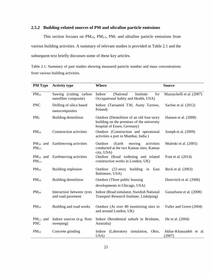
2.5.2 Building-related sources of PM and ultrafine particle emissions
This section focuses on PM10, PM2.5, PM1 and ultrafine particle emissions from
various building activities. A summary of relevant studies is provided in Table 2.1 and the
subsequent text briefly discusses some of these key articles.
Table 2.1: Summary of past studies showing measured particle number and mass concentrations
from various building activities.
PM Type Activity type Where Source
PM10 Sawing (cutting carbon
nanofibre composite)
Indoor (National Institute for
Occupational Safety and Health, USA)
Mazzuckelli et al. (2007)
PNC Drilling of silica based
nanocomposites
Indoor (Tarnamid T30, Azoty Tarnow,
Poland)
Sachse et al. (2012)
PM1 Building demolition Outdoor (Demolition of an old four-story
building on the premises of the university
hospital of Essen, Germany)
Hansen et al. (2008)
PM10 Construction activities Outdoor (Construction and operational
activities a port in Mumbai, India )
Joseph et al. (2009)
PM10 and
PM2.5
Earthmoving activities Outdoor (Earth moving activities
conducted at the two Kansas sites, Kansas
city, USA)
Muleski et al. (2005)
PM10 and
PM2.5
Earthmoving activities Outdoor (Road widening and related
construction works in London, UK)
Font et al. (2014)
PM10 Building implosion Outdoor (22-story building in East
Baltimore, USA)
Beck et al. (2003)
PM10 Building demolition Outdoor (Three public housing
developments in Chicago, USA)
Dorevitch et al. (2006)
PM10 Interaction between tyres
and road pavement
Indoor (Road simulator, Swedish National
Transport Research Institute, Linköping)
Gustafsson et al. (2008)
PM10 Building and road works Outdoor (At over 80 monitoring sites in
and around London, UK)
Fuller and Green (2004)
PM2.5 and
PNC
Indoor sources (e.g. floor
sweeping)
Indoor (Residential suburb in Brisbane,
Australia)
He et al. (2004)
PM10 Concrete grinding Indoor (Laboratory simulation, Ohio,
USA)
Akbar-Khanzadeh et al.
(2007)

22
Concrete drilling, crushing and cutting are common activities both at construction sites
and within domestic situations, and have the potential to generate significant airborne dust
(Cook Jr and Harris, 1992; Kumar et al., 2012c). This is probably due to the higher
rotational frequency, shear stresses and local energy density associated with drilling,
crushing and cutting activities. Some studies have focused on PM10 (Akbar-Khanzadeh and
Brillhart, 2002) and PM2.5 (Flower and Sanjayan, 2007) and ultrafine particles (Kumar et
al., 2012c) created during concrete grinding, manufacturing and crushing activities,
respectively. For example, Kumar et al. (2012c) investigated the emission of ultrafine
particles by simulating building activities, such as crushing concrete blocks in the
laboratory environment and found notable quantities of ultrafine particles (2.27±0.41 ×10⁴
cm-3) compared to the background level (1.40±0.40 ×104 cm-3). Despite the fact that such
activities are undertaken on a daily basis around the world, surprisingly little is known
about the associated exposure levels and physicochemical features of the particles
produced (Broekhuizen et al., 2011). Further literature reviews on concrete mixing, drilling
and cutting are provided in Chapter 4.
Building refurbishment or renovation typically includes bringing older buildings up to
modern standards for improving lighting, heating and energy efficiency, as well as
upgrading outdated buildings (Mickaityte et al., 2008; Sunikka and Boon, 2003). Activities
related to building refurbishment have already grown in number in most European
countries over the last 20 years (Kohler and Hassler, 2002), due to the increase in the rate
of population growth within urban areas (Egbu, 1999). Refurbishment activities can have
an associated carbon footprint of the order of 20% of the emissions that arose from the

23
original construction (Pacca and Horvath, 2002). However, the contribution of the building
refurbishment activities to PM10, PM2.5, PM1 and ultrafine particles and also the extent of
the pollution caused due to refurbishment activities is still unknown. Further literature
reviews on building refurbishment works are presented in Chapter 5.
Construction works involve the processes of building a structure or a facility in ways
known to result in incremental increase of PM10 local concentrations, which may contain a
wide variety of toxic and harmful substances and may adversely impact the health of nearby
residents (Anderson, 2009; Davila et al., 2006; Heal et al., 2012; Loomis, 2000). These
increments in PM10 concentration are typically thought to be due to construction activities
including the resuspension of dust from any on-site vehicles at the construction sites. There
are a few studies concerned with emissions of PM10 arising from outdoor construction
works (Fuller and Green, 2004; Joseph et al., 2009; Font et al., 2014), but there is still very
little work focusing on the fractions of PM2.5 produced from construction activities
(Muleski et al., 2005). For example, Fuller and Green (2004) studied the emission of PM10
particles generated by construction works in London, UK. It was found that the PM10
concentrations breached the 24-h mean EU limit (50 μg m−3) for PM10 concentrations on
numerous occasions at 25% of the monitoring stations. Further details of the literature on
construction activities are provided in Chapter 6.
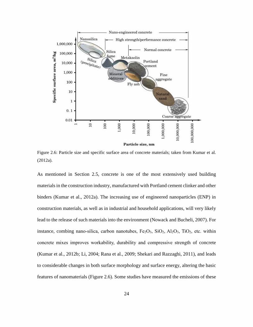
24
Figure 2.6: Particle size and specific surface area of concrete materials; taken from Kumar et al.
(2012a).
As mentioned in Section 2.5, concrete is one of the most extensively used building
materials in the construction industry, manufactured with Portland cement clinker and other
binders (Kumar et al., 2012a). The increasing use of engineered nanoparticles (ENP) in
construction materials, as well as in industrial and household applications, will very likely
lead to the release of such materials into the environment (Nowack and Bucheli, 2007). For
instance, combing nano-silica, carbon nanotubes, Fe2O3, SiO2, Al2O3, TiO2, etc. within
concrete mixes improves workability, durability and compressive strength of concrete
(Kumar et al., 2012b; Li, 2004; Rana et al., 2009; Shekari and Razzaghi, 2011), and leads
to considerable changes in both surface morphology and surface energy, altering the basic
features of nanomaterials (Figure 2.6). Some studies have measured the emissions of these

25
nano-sized particles through different generation methods (Tsai et al., 2012; Tsai et al.,
2009) and a number of other studies have investigated exposure to them during handling
and bagging processes at workplaces (Fujitani et al., 2008; Brouwer, 2010; Tsai et al.,
2011).
Building demolition is the tearing-down of buildings and other structures, which involves
taking a building apart while carefully preserving valuable elements for re-use. Each year,
the number of buildings demolished is expected to growth by 4-time by 2016 in the UK
from the levels of about 20,000 per year in 2008 (ECI, 2005; Roberts, 2008), in order to
meet new building technology and urban design guidelines (Balaras et al., 2007; Kumar et
al., 2015). Demolition and construction waste contribute about 33% of the total waste from
all sectors, which about half of it is demolition waste (Balaras et al., 2007). Building
demolition can be accomplished either mechanically or through implosion. Particles are
then produced during the breaking up and demolition of building materials such as concrete
slabs, iron beams, brick walls and also the shifting of the waste building material from the
site that may lead to resuspension and further generation of particles. Demolition by both
mechanical disruption (Dorevitch et al., 2006) and implosion (Beck et al., 2003) has the
potential to produce significant amounts of PM10, but still much less is known about PM2.5
and PM1, and also the impact of building demolition on the air quality of the surrounding
areas (Beck et al., 2003). Further review of the literature on building works are presented
in Chapter 7.
Recycling of construction waste is one of the effective ways to manage the related
environmental problems, and also helps to save the limited space available of landfill

26
(Nakamura and Kondo, 2002). The enormous amount of construction and demolition waste
produced reached a level where warnings about use were made. Among various types of
materials, concrete waste accounts for about 50% of the total construction and demolition
waste generated (Tam, 2008). After concrete structures are demolished or renovated,
concrete recycling is an increasingly common method of utilising the rubble and remaining
aggregates (Dosho, 2007; Rao et al., 2007). Aggregate recycling of concrete waste is a
cost-effective method which can help the environment. However, there are a limited
number of studies concerned with the exposure to particles generated by concrete recycling
and the associated risks to the workers at recycling sites. For example, Kumar and
Morawska (2014) investigated the exposure to ultrafine particles by simulating a concrete
recycling activity and found significant exposure rate to be 24.83×10⁸ min–1 during
measurements close to the source.
Earthworks cover the processes of soil-stripping, ground-levelling, excavation and
landscaping. Common earthworks take place in roads, railway beds, causeways, dams,
levees, canals, and berms (Smith et al., 2000). For example, Muleski et al. (2005) measured
PM10 during the earth moving, track loading and track out works in Kansas, USA. Average
PM10 emission factors were reported for earthmoving works (~0.41 kg veh-1 km-1), track
loading (~0.06 kg mg-1) and track out works (~0.006 kg veh-1), respectively. Track out is
the transporting of dust and materials waste from the construction site onto the public road
network, where it can be deposited and then re-suspended by vehicles using the network.
This activity can take place when lorries leave the construction or demolition site with
dusty materials which may then spill onto the road (Muleski et al., 2005). There are also a
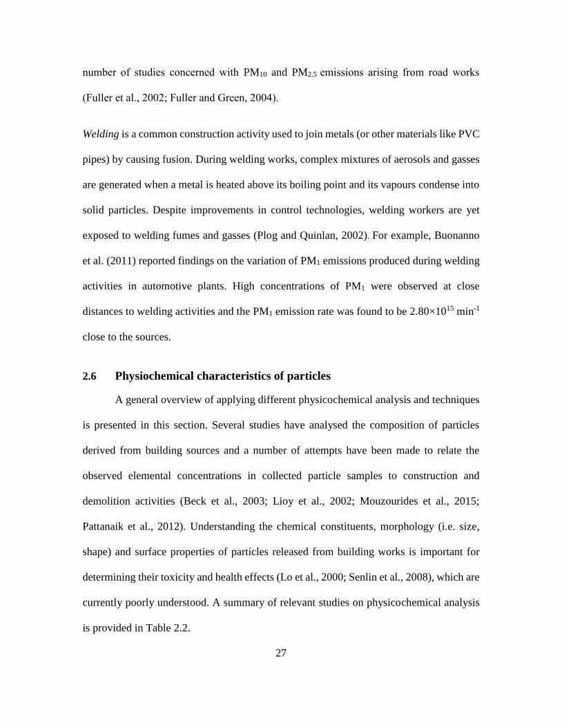
27
number of studies concerned with PM10 and PM2.5 emissions arising from road works
(Fuller et al., 2002; Fuller and Green, 2004).
Welding is a common construction activity used to join metals (or other materials like PVC
pipes) by causing fusion. During welding works, complex mixtures of aerosols and gasses
are generated when a metal is heated above its boiling point and its vapours condense into
solid particles. Despite improvements in control technologies, welding workers are yet
exposed to welding fumes and gasses (Plog and Quinlan, 2002). For example, Buonanno
et al. (2011) reported findings on the variation of PM1 emissions produced during welding
activities in automotive plants. High concentrations of PM1 were observed at close
distances to welding activities and the PM1 emission rate was found to be 2.80×10¹⁵ min-1
close to the sources.
2.6 Physiochemical characteristics of particles
A general overview of applying different physicochemical analysis and techniques
is presented in this section. Several studies have analysed the composition of particles
derived from building sources and a number of attempts have been made to relate the
observed elemental concentrations in collected particle samples to construction and
demolition activities (Beck et al., 2003; Lioy et al., 2002; Mouzourides et al., 2015;
Pattanaik et al., 2012). Understanding the chemical constituents, morphology (i.e. size,
shape) and surface properties of particles released from building works is important for
determining their toxicity and health effects (Lo et al., 2000; Senlin et al., 2008), which are
currently poorly understood. A summary of relevant studies on physicochemical analysis
is provided in Table 2.2.

28
Table 2.2: Summary of physicochemical analysis of particles collected during number of building-
related activities.
2.6.1 Scanning electron microscopy (SEM)
A SEM is a type of electron microscope that produces images of a sample by
scanning it with a focused beam of electrons. Various signals are produced due to the
interaction between the electrons and atoms that can be detected, and which contain
information about an examined sample's surface composition and topography. A very fine
probe of electrons with energies from a few hundred eV to tens of KeV is focused at the
surface of the specimen and scanned across it in a raster or pattern of parallel lines. Signals
Activity type Technique used Description Source
Building
destruction
SEM-EDS It was found that the majority of
particles were composed of building-
related materials such as Ca, Si and S
McGee et al. (2003)
Building implosion XRF The elemental composition of
particles collected in samples was
dominated by Ca, Si, Al and Fe
Beck et al. (2003)
Building
destruction
TEM/SEM-EDS Elements such as Si (dominant), Ca, S,
Zn, Al and Mg were found in collected
samples
Lioy et al. (2002b)
Welding TEM/SEM-EDS Fe (dominant), Mn, S, K and Ca were
found during analysis of welding fume
particles
Jenkins and Eagar
(2005)
Welding TEM-PIXE Elements such as Fe (dominant), Mn,
Ni, and Cr were found during analysis
of welding fume particles
Isaxon et al. (2009)
Drilling TEM/SEM-EDS The elemental composition was
dominated by Zn, Si, Al and Fe via
analysis of collected particles
Bello et al. (2010)
Grinding SEM-EDS and
ICP-MS
The presence of elements such as Fe,
Cr, Mn, Si and Ni were found in
samples collected during grinding
activity
Iavicoli et al.
(2013)

29
are amplified and used to vary the brightness of the trace on a cathode ray tube being
scanned in synchrony with the probe. There is thus a direct positional correspondence
between the electron beam scanning across the specimen and the fluorescent image on the
cathode ray tube.
Mass measurements can now be carried out regularly on a wide range of molecular
structures utilising elastically scattered electrons (Engel and Colliex, 1993). Recent
progress in the acquisition and analysis of electron energy-loss spectroscopy data indicates
that the scanning transmission electron microscope is an efficient tool for mapping the
chemical composition of a biological sample. A few studies have utilised SEM for
examining the solid-phase of metals and metalloids in house dust (Walker et al., 2011),
determining the specific sources of lead in both household dust (Hunt et al., 1992) and the
laser cleaning of building stones (Potgieter-Vermaak et al., 2005). Scanning electron
microscopy together with focused ion beam milling (FIB-SEM) has been used to
investigate the composition of atmospheric particles (Conny, 2013).
2.6.2 Energy-dispersive X-ray spectroscopy (EDS)
There are also techniques such as SEM for analysing morphology and the energy
dispersive X-ray spectroscopy technique (EDS) to find elemental composition, which are
used by numerous environmental studies (Kupiainen et al., 2003; Mouzourides et al., 2015;
Paoletti et al., 2002). For example, Mouzourides et al. (2015) assessed the characteristics
of bulk PM samples collected on polytetrafluoroethylene (PTFE) filters at an urban air
pollution monitoring station in Nicosia (Cyprus) using SEM and EDS techniques. The
results showed the presence of elements such as calcium (Ca), nitrogen (N) and lead (Pb)

30
in the samples. Likewise, Paoletti et al. (2002) studied the physicochemical characteristics
and composition of particles in an urban area of Rome (Italy). They observed that elements
such as carbon (C) and nitrogen (N) mainly originated from vehicular sources. McGee et
al. (2003) also used SEM/EDS analysis to analyse the particles collected during the
destruction of the World Trade Centre that caused the release of high levels of PM into the
local environment in New York (USA). It was found that the majority of particles were
composed of building related materials such as calcium (Ca), silicon (Si) and sulphur (S)
(McGee et al., 2003). Currently, only a limited number of studies have reported
physicochemical properties of particles released from building sources and therefore this
is taken up for investigation in this thesis.
2.6.3 Ion Beam Analysis (IBA)
The conjunction of Particle Induced X-ray Emission (PIXE) and Elastic
Backscattering Spectrometry (EBS) techniques represent powerful tools for measuring the
elemental composition of fine atmospheric particles sampled on filters, as have been
applied by Saitoh et al. (2003) during chemical characterisation of PM10 and PM2.5 in diesel
exhaust particles at the National Traffic Safety and Environment Laboratory in Tokyo
(Japan). The major components of PM10 and PM2.5 were found to be sodium (Na), silicon
(Si), magnesium (Mg), chlorine (Cl), sulphur (S), iron (Fe), calcium (Ca) and zinc (Zn) as
a result of the analysis. Similarly, Kothai et al. (2009) analysed the elemental composition
of atmospheric PM at Vashi in Mumbai (India) and found the presence of components such
as copper (Cu), chromium (Cr) and manganese (Mn) during the PIXE analysis, suggesting
that they originated from anthropogenic sources. Despite these studies there remains a

31
considerable research gap with respect to the presence of elements such as arsenic (As),
cadmium (Cd), chromium (Cr), lead (Pb), nickel (Ni), manganese (Mn) and zinc (Zn)
within the particles arising from building activities.
2.6.4 X-ray Photoelectron Spectroscopy (XPS)
XPS is the most widely used surface analysis technique due to its relative simplicity
of use and the ease of data interpretation. XPS has been demonstrated to be a powerful
technique for examining the surface characteristics of various materials. XPS can perform
elemental analysis for essentially the entire periodic table. The technique is surface-
sensitive because the electrons whose energies are analysed arise from a depth of no greater
than about 2-5 nm (He et al., 2007). Those electrons which are photo-excited, and which
escape without loss of energy contribute to the characteristic peaks in the spectrum; those
which suffer inelastic scattering and suffer energy loss contribute to the background of the
spectrum. After a photoelectron has been emitted, the ionised atom must relax in some
way. This can be achieved by the emission of an X-ray photon. The other option is the
ejection of an electron as an Auger electron. Both types of relaxation are shown in
Figure 2.7 (Watts, 1990). Several studies have been conducted using XPS to analyse the
composition of particles derived from those sources which may contribute trace elements
to urban aerosols and a number of attempts have been made to relate the observed elemental
concentrations in collected aerosol samples to these sources (Adhami et al., 2012;
Batonneau et al., 2004; Chen et al., 2000; Pattanaik et al., 2012; Roguala-Kozlowska et al.,
2008). For example, Roguala-Kozlowska et al. (2008) studied the influence of vehicular
traffic on the particle surface composition of PM10 and PM2.5 in Zabrze (Poland) and found
that the main components of the surface layer of these particles were carbon (C), nitrogen
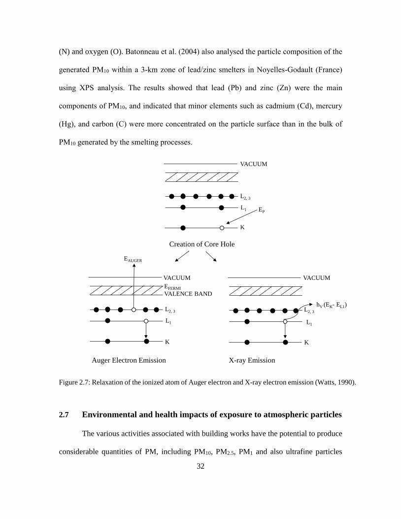
32
(N) and oxygen (O). Batonneau et al. (2004) also analysed the particle composition of the
generated PM10 within a 3-km zone of lead/zinc smelters in Noyelles-Godault (France)
using XPS analysis. The results showed that lead (Pb) and zinc (Zn) were the main
components of PM10, and indicated that minor elements such as cadmium (Cd), mercury
(Hg), and carbon (C) were more concentrated on the particle surface than in the bulk of
PM10 generated by the smelting processes.
Figure 2.7: Relaxation of the ionized atom of Auger electron and X-ray electron emission (Watts, 1990).
2.7 Environmental and health impacts of exposure to atmospheric particles
The various activities associated with building works have the potential to produce
considerable quantities of PM, including PM10, PM2.5, PM1 and also ultrafine particles
Creation of Core Hole
Auger Electron Emission X-ray Emission
VACUUM VACUUM
VACUUM
L2, 3
L1
L1 L1
L2, 3 L2, 3
K
K
K
EP
EAUGER
EFERMI
VALENCE BAND
hV (EK- EL1)

33
(Kumar et al., 2012b, 2013b). These particles have serious environmental and health-
related consequences because they may contain a variety of toxic organic and metallic
compounds (Heal et al., 2012). Details about the impacts of exposure to PM10, PM2.5, PM1
and also ultrafine particles on health, visibility and climate change are discussed in the
following sections.
2.7.1 Health effects
PM10 in the urban environment is harmful since it can easily be introduced into the
respiratory system (Davila et al., 2006), although PM2.5 has been recognised as the 9th most
powerful risk factor for disease globally (Lim et al., 2012). A number of epidemiological
studies have shown that excess mortality comes from exposure to PM10 and PM2.5 particles
from sources such as road traffic and industry (Janssen et al., 2013; Kan et al., 2007;
Namdeo and Bell, 2005). Furthermore, excessive inhalation of PM10 has been linked to a
variety of respiratory diseases, such as lung cancer (Turner et al., 2011; Vineis et al., 2004)
and asthma (Dorevitch et al., 2006; Eggleston et al., 1999). Also, a number of studies have
linked excessive inhalation of PM2.5 to renal (Spencer-Hwang et al., 2011; Weng et al.,
2015) and cardiovascular diseases (Brook et al., 2010; Peng et al., 2008). There is also an
increasing interest in the risks of PM1 and ultrafine particles since these penetrate deeper
into the lungs and are thought to be of greater concern for human health (Chaloulakou et
al., 2003) as PM10 and PM2.5 tend to penetrate into the gas exchange regions of the lung,
but PM1 and ultrafine particles can pass through the lungs to affect cells, tissues and organs
of body. Number of studies have also confirmed the link between PM1 exposure and
morbidity (Pope and Dockery, 2006), and to several health issues such as cardiopulmonary
(Zereini et al., 2012) and pulmonary diseases (Ostro et al., 2010). The smaller size of

34
ultrafine particles compared with PM1 enables them to enter deeper into lungs, causing
both acute and chronic adverse health effects such as asthma, and also cardiovascular and
ischemic heart diseases (Goel and Kumar, 2014). However, the exact number of excess
deaths and higher mortality rate due to exposure to ultrafine particles in the urban
environment is yet unknown (Kumar et al., 2014).
Numerous studies have also reported the increased risk of death caused by PM10 and PM2.5
due to ischemic heart disease among construction welders, plasterers and masons (Cavallari
et al., 2007; Sjögren et al., 2002; Stern et al., 2001). PM10 and PM2.5 have kinetic features,
which mean they can be deposited in different internal parts of the body through the
respiratory system and also can be translocated in the body through the circulatory system
which supplies blood to the heart, liver and kidneys (Kampa and Castanas, 2008). Similar
adverse health effects have even been observed among non-smoking workers at
construction sites (Bergdahl et al., 2004; Verma et al., 2003), as well as depression
problems among construction workers (Haynes and Savage, 2007). Some studies have
shown that workers in construction and demolition industry dealing directly with cement
and concrete materials are exposed to considerable PM10 and PM2.5 emissions (Croteau et
al., 2002; Flanagan et al., 2006) compared with those working in other industries such as
the wood and metal industries (Fischer et al., 2005; Lim et al., 2010). Air pollution due to
PM10, PM2.5, PM1 and ultrafine particles from building activities can also adversely affect
the health of people living close to the operation sites, particularly where measures to
restrict and limit the amount of particles produced from the sites are insufficient (Kumar et
al., 2012b). Hence, estimating the level of PM2.5, PM1 and ultrafine particles exposure

35
becomes even more important when such sites are situated within sensitive areas such as
in the vicinity of hospitals and schools, or in densely built residential areas.
2.7.2 Visibility and climate change
There is sufficient evidence that building-related works such as earthmoving,
building renovation and demolition considerably degrade the air quality of the surrounding
environment (Beck et al., 2003; Font et al., 2014; Hansen et al., 2008; Joseph et al., 2009;
Muleski et al., 2005). One of the most obvious indicators of air quality is visibility.
Visibility is defined as the furthest distance in a given direction at daytime at which it is
just possible to see and identify a prominent dark object against the skyline with the unaided
eye (Tao et al., 2007). A number of studies have demonstrated that visibility is significantly
influenced by the chemical composition, size and concentration of particles (Cheng and
Tsai, 2000; Cheung et al., 2005). Nitrate and sulphate, which are generally formed at a
considerably quicker rate in water droplets under high humidity conditions, are the main
reasons for degraded the visibility (Mangelson et al., 1997; Tang and Munkelwitz, 1994).
In rural regions of Europe, good visibility is usually considered to be 40-50 km, though
anthropogenic works mainly account for reduction of visibility in urban areas (Horvath,
1995; Kim et al., 2001). Reduction in visibility is a result of processes such as light
absorption by water vapor and scattering by aerosol particles such as PM10, PM2.5 and PM1
(Majewski et al., 2014). Several studies have reviewed the impact of PM10 (Vajanapoom
et al., 2001; Wan et al., 2012), PM2.5 (Abby et al., 1994; Zhang et al., 2006) and PM1
(Sabbagh-Kupelwieser et al., 2010; Shi et al., 2014) on decreasing visibility of the
surrounding enviroment. For example, Wan et al. (2012) investigated the air quality impact
of PM10 on atmospheric visibility in the Pearl River Delta (China) and found that visibility

36
was reduced to less than 8 km 22% of the time from 1998 to 2008, mainly due to PM10
emissions.
Climate change is a change in the statistical distribution of weather patterns and may refer
to a change in average weather conditions, or a change in the time variation of weather
based on longer-term average conditions. The effect of aerosols such as PM10 (D’amato et
al., 2010), PM2.5 (Tai et al., 2010), PM1 (Vecchi et al., 2004), ultrafine particles (Feng et
al., 2011) and greenhouse gasses (Meinshausen et al., 2009) is estimated through their
global warming potential, which provides a measure of an aerosol’s effect on global climate
change relative to that of CO2 for a given duration (Pearce et al., 1996). Generally, it is
thought that aerosols change the radiative properties of the atmosphere and represent net
negative radiative forcing, such as a cooling effect on climate and on the Earth’s
temperature. For example, PM10 particles may affect the earth’s temperature by their effect
on scattering the incoming solar radiation as they are bigger than the other particles in size
with shorter lifetime in the air (Tiwari et al., 2009). PM2.5 in the urban environment also
mainly consists of black carbon, which is formed due to incomplete combustion of fossil
fuels and biomass. PM2.5 can stay in the atmosphere for several days or even weeks, which
may cause a rise in the temperature of the Earth by absorbing sunlight and reducing albedo
when deposited on snow (Lonati et al., 2007). PM1 also affects the natural energy balance
of the Earth, largely by reflecting and absorbing solar radiation, but also by influencing the
reflective and absorbing features of clouds through condensation (Vecchi et al., 2004).
However, the uncertainties relating to the direct effects of ultrafine particles on climate
change remain significant and difficult to verify at the present time. However, in order to

37
control the rise in global temperature it is important to control the PM10, PM2.5, PM1,
ultrafine particles and greenhouse gas emissions, as greenhouse gasses have a much longer
lifetime in the atmosphere (Coakley et al., 1983). Because of the above-mentioned health
impacts and other problems such as acid rain, regulatory authorities must now more
carefully control particulate emissions from building, vehicular and industrial sources,
thereby leading to a rapid improvement in local air quality (Schopp et al., 1998).
2.8 Regulations, guidance and limits for PM and ultrafine particles
Environmental and health concerns associated with dust inhalation have led to a
number of reduction and control initiatives of PM10, PM2.5, PM1 and ultrafine particles in
the construction and demolition industries. The UK Health and Safety Executive (HSE)
has provided good practice guidelines to control and limit exposure to hazardous materials
and substances at construction and demolition sites (HSE, 2006, 2011). Moreover, in the
UK ‘Best Practice Guidance’ has been produced by London Councils at the local level, in
partnership with the Greater London Authority which include a number of practical
methods to control dust and emissions from construction and demolition works (Authority
and Councils, 2006). In the US, the United States Environmental Protection Agency
(USEPA) has provided guidelines on specific emission factors for different activities such
as construction, demolition and mineral operations to control and limit PM emissions
(EPA, 2011). These emission inventories are discussed further in Section 7.3.5. However,
construction and demolition sites can be situated within very busy places, where meeting
regulatory expectations and guidelines can often be challenging. Further details on the limit
values of particles are provided in Table 2.3. Moreover, targets have been set by the

38
European Union Directive (1999) for year 2004 and 2010 to limit daily and annual mean
values of PM10 at the European-wide level (Fuller and Green, 2004). For example, the limit
by 2005 was to achieve a daily mean PM10 concentration of 50 µg m-3, not to be exceeded
on more than 35 occasions per year, and annual mean values of 40 µg m-3. In addition, the
target by 2010 was to achieve daily mean PM10 concentration of 50 µg m-3, not to be
exceeded on more than 7 occasions per year, and annual mean concentrations of 20 µg m-
3. However, the target values to be met by 2010 were not carried into Directive 2008/50/EC
(Directive, 2008). Furthermore, a legal limit value for the three-year mean PM2.5
concentration has been proposed by the EU, which cannot exceed of 25 µg m-3 by 2015
(Directive, 2008). In addition, World Health Organisation (WHO) guidelines (WHO, 2006)
propose that the annual and daily mean concentrations of PM10 and PM2.5, should not
exceed (20 and 50 µg m-3) and (10 and 25 µg m-3), respectively. Table 2.3 presents the
ambient PM standards enforced by the EU, USEPA, WHO, Japan and India. There are
currently no national or international regulations or limits for controlling the release of PM1
and ultrafine particles on buildings sites (Kumar et al., 2012c).
There are also number of studies available that quantify the level of exposure workers
experience in workplace environments (e.g. coal- and gas-fired power plant workplaces)
where PM10 (Stephenson et al., 2003), PM2.5 (Kousa et al., 2002b), PM1 (Hicks et al., 2012)
and ultrafine particles (Methner et al., 2010) are produced. However, only limited
guidelines, such as those produced by WHO and HSE, are available for controlling
exposure to particles in workplaces. For example, the HSE recommended controlling
exposure at source by carrying out all tasks, including packaging disposal, in a ducted fume

39
cupboard with a high efficiency particulate air filter (HEPA) and using another effective
local exhaust ventilation, with a HEPA filter. In addition, HSE presented more
recommendations by providing Control of Substances Hazardous to Health (COSHH) and
Work Exposure Limits (WEL) guiltiness, which require employers to control workers’
exposure to substances hazardous to health.
Table 2.3: Summary of ambient air quality limits and standards; (Directive, 2008; EPA, 2011;
WHO, 2006; CPCB, 2010; Kumar, 2009). Please note that N.S. refers to not specified.
PM
(µg m-3)
Arithmetic
Mean
EU WHO USEPA Japan India
(Residential areas)
PM10 Annual mean 40 20 Revokedc N.S 60g
24-hour mean 50a 50 150d 50 100h
PM2.5 Annual mean 25b 10 15e N.S 40g
24-hour mean N.S 25 35f N.S 60h
PM1 Annual mean N.S N.S N.S N.S N.S
24-hour mean N.S N.S N.S N.S N.S
a The EU Directive 2008/50/EC stipulated that annual mean values of PM10 should not exceed a
24-hour mean of greater than 50 µgm-3 more than 35 days in a year.
b Three-year mean PM2.5 concentration cannot exceed of 25 µg m-3.
c The USEPA agency revoked the annual PM10 standard in 2006.
d Not to be exceeded more than once per year on average over 3 years.
e To attain this standard, the 3-year average of the weighted annual mean PM2.5 concentrations must
not exceed 15 μg m–3.
f To attain this standard, the 3-year average of the 98th percentile of 24-h concentrations area must
not exceed 35 μg m–3.
g Annual Arithmetic mean of minimum 104 measurements in a year at a particular site taken twice
a week 24 hourly at uniform intervals.
h 24 hourly 8 hourly or 1 hourly monitored values, as applicable shall be complied with 98% of the
time in a year. 2% of the time, they may exceed the limits but not on two consecutive days of
monitoring.

40
2.9 Chapter summary
This chapter has provided detailed information about the background to and
primary concept of airborne PM and ultrafine particles. This chapter has reviewed the
studies related to mass and number concentrations, particle distribution, sources of particle
emissions, instrumentation, physicochemical analysis, exposure to the particles, health
effects and current regulations. This review has suggested that adverse environmental and
health effects can be expected with exposure to PM10, PM2.5, PM1 and ultrafine particles at
high mass and number concentrations. Several studies mentioned in this chapter
highlighted the importance of PM and ultrafine particles emissions from building sources.
The chapter has also covered the physicochemical characteristics of particles including
their morphology and composition, using different form of analysis. The chapter concluded
with a discussion of the potential impacts of PM and ultrafine particles on the surrounding
environment and considered the associated regulations for controlling particle emissions.
This chapter has highlighted the lack of studies about the release of airborne PM and
ultrafine particles from major building activities such as construction, demolition and
refurbishment, while acknowledging that numerous studies are available on dust emissions
from different sources, such as vehicles and industrial sources. Further researches are
needed to develop appropriate regulations for the control of PM10, PM2.5, PM1 and ultrafine
particles arising from building works in order to provide adequate protection for on-site
workers and individuals living in nearby neighbourhoods. However, these investigations do
not stop here, as further literature reviews are provided in the following chapters that relate to
each individual objective.

41
Chapter 3. Materials and methods
This chapter presents a set of methods, instruments descriptions and the physicochemical
analysis intended for achieving the research objectives.
3.1 Introduction
Experiments were conducted in the controlled laboratory, indoor and outdoor field
sites, to study the emissions of PM10, PM2.5, PM1 and ultrafine particles during building-
related works such as concrete mixing, drilling, cutting, refurbishment, construction and
demolition, as described in Section 1.3. The experimental studies in this section provide
information on particle emission rates, together with methods used to calculate the
respiratory deposition doses and physicochemical features including the morphology and
chemical compositions of particles. Measuring particles in the required size range was
performed using a DMS50 for measurements of PNCs and PNDs and using GRIMM (1.107
E), TEOM (1400) and OSIRIS (2315) instruments for measuring PMCs and PMDs (Table
3.1). A Kestrel 4500 weather station was also used to measure meteorological data (wind
speed, direction, relative humidity and ambient temperature) at the measurement site.
Furthermore, samples were collected on PTFE filters, and each of these samples was
analysed using SEM, EDS, XPS and IBA analysis. The detailed descriptions of these
instruments and their working principles are presented in the subsequent section, Section
3.2.
42
Table 3.1: Summary of the instruments used for measuring PM10, PM2.5, PM1 and ultrafine particles
during experiments.
3.2 Instrumentation
3.2.1 GRIMM (1.107 E)
A GRIMM particle spectrometer (model 1.107 E) was used to measure the mass
distribution of particles per unit volume of air in 15 different channels covering the 0.2–
20 µm in size range (Goyal and Kumar, 2013). The sensitivity of the instrument is 1 µg
m–3, and instrument reproducibility of size-resolved PMC is ±2% over the total measuring
range. Optical signals pass through a multichannel size classifier to a pulse height analyser
that classifies the signals based on size into appropriate channels. Ambient air was drawn
into the unit every 6 second via an internal volume-controlled pump at a rate of 1.2 lit min–
1 (Goyal and Kumar, 2013; Grimm and Eatough, 2009).
Two cross validation approaches were used to ensure the quality of the collected data.
Firstly, the instrument was calibrated in a three-step process by the manufacturer prior to
the on-site measurements, including verification of laser optics, gravimetric correlation
verification and optical calibration against the known size-resolved distribution, density
Work type Chapter number Instrument used Size range (µm)
Simulated laboratory investigations Chapter 4 DMS50
GRIMM (1.107 E)
0.005–5
0.2–20
Indoor refurbishment measurements Chapter 5 DMS50
GRIMM (1.107 E)
0.005–5
0.2–20
Outdoor construction measurements Chapter 6 TEOM (1400)
OSIRIS (2315)
0.1–10
0.4–20
Outdoor demolition measurements Chapter 7 GRIMM (1.107 E) 0.2–20
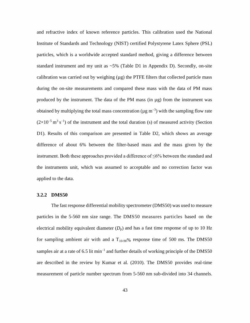
43
and refractive index of known reference particles. This calibration used the National
Institute of Standards and Technology (NIST) certified Polystyrene Latex Sphere (PSL)
particles, which is a worldwide accepted standard method, giving a difference between
standard instrument and my unit as ~5% (Table D1 in Appendix D). Secondly, on-site
calibration was carried out by weighing (µg) the PTFE filters that collected particle mass
during the on-site measurements and compared these mass with the data of PM mass
produced by the instrument. The data of the PM mass (in µg) from the instrument was
obtained by multiplying the total mass concentration (µg m–3) with the sampling flow rate
(2×10⁻⁵ m3 s–1) of the instrument and the total duration (s) of measured activity (Section
D1). Results of this comparison are presented in Table D2, which shows an average
difference of about 6% between the filter-based mass and the mass given by the
instrument. Both these approaches provided a difference of ≤6% between the standard and
the instruments unit, which was assumed to acceptable and no correction factor was
applied to the data.
3.2.2 DMS50
The fast response differential mobility spectrometer (DMS50) was used to measure
particles in the 5-560 nm size range. The DMS50 measures particles based on the
electrical mobility equivalent diameter (Dp) and has a fast time response of up to 10 Hz
for sampling ambient air with and a T10-90% response time of 500 ms. The DMS50
samples air at a rate of 6.5 lit min–1 and further details of working principle of the DMS50
are described in the review by Kumar et al. (2010). The DMS50 provides real-time
measurement of particle number spectrum from 5-560 nm sub-divided into 34 channels.
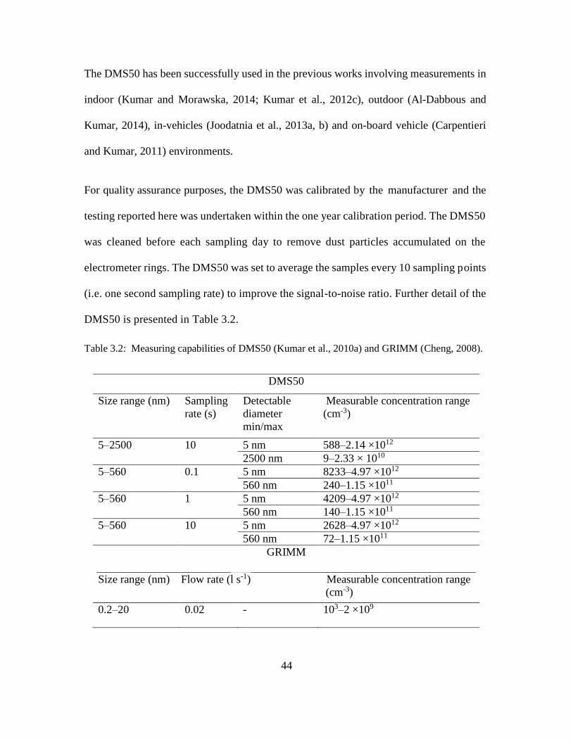
44
The DMS50 has been successfully used in the previous works involving measurements in
indoor (Kumar and Morawska, 2014; Kumar et al., 2012c), outdoor (Al-Dabbous and
Kumar, 2014), in-vehicles (Joodatnia et al., 2013a, b) and on-board vehicle (Carpentieri
and Kumar, 2011) environments.
For quality assurance purposes, the DMS50 was calibrated by the manufacturer and the
testing reported here was undertaken within the one year calibration period. The DMS50
was cleaned before each sampling day to remove dust particles accumulated on the
electrometer rings. The DMS50 was set to average the samples every 10 sampling points
(i.e. one second sampling rate) to improve the signal-to-noise ratio. Further detail of the
DMS50 is presented in Table 3.2.
Table 3.2: Measuring capabilities of DMS50 (Kumar et al., 2010a) and GRIMM (Cheng, 2008).
DMS50
Size range (nm) Sampling
rate (s)
Detectable
diameter
min/max
Measurable concentration range
(cm-3)
5–2500 10 5 nm 588–2.14 ×10¹²
2500 nm 9–2.33 × 10¹⁰
5–560 0.1 5 nm 8233–4.97 ×10¹²
560 nm 240–1.15 ×10¹¹
5–560 1 5 nm 4209–4.97 ×10¹²
560 nm 140–1.15 ×10¹¹
5–560 10 5 nm 2628–4.97 ×10¹²
560 nm 72–1.15 ×10¹¹
GRIMM
Size range (nm) Flow rate (l s-1) Measurable concentration range
(cm-3)
0.2–20 0.02 - 103–2 ×10⁹

45
3.2.3 OSIRIS (2315)
Turnkey’s Osiris instrument (model 2315) was used to measure the mass
distribution of particles per unit volume of air in the 0.4 to 20 µm size range by light
scattering technology in a mass concentration range of 0.1 to 6000 µg m–3 (Tasic et al.,
2012). The Osiris is a portable device that is capable of sampling and measuring particle
concentrations in real-time at high temporal resolution (1 s minimum). The air sample is
continuously drawn into the instrument by a pump with a flow rate set by the
microprocessor at a rate of 0.6 l min–1 through an inlet heated to 50 °C to minimise the
effects of water droplets and particle bound water. Over 20,000 particles a second can be
sized before coincidence effects occur. Several size selective inlets are also available for
the instrument. These can be used to collect a size selected gravimetric sample on the
instrument’s filter and will measure in μg m-3. Osiris also allows wind speed and direction,
temperature and relative humidity to be recorded at the same time. Turnkey Instruments,
OSIRIS monitors, have also been used for the assessment of indoor and outdoor PM levels
as well as personal exposure in a number of past studies (Gulliver and Briggs, 2004a; Kim
et al., 2008).
3.2.4 TEOM (1400)
The TEOM 1400 was used to measure mass of particles per unit volume of air in
the size range of 0.1–10 µm. The instrument was capable of measuring particle mass
concentration in the 0 to 1,000,000 µg m–3 range with a mass flow rate of 3 l min–1 (Cyrys
et al., 2001). The sampling stream and filters were heated to 50 °C to maintain a stable
temperature and eliminate interference from water on the filter. The mass measurement
46
relied on the measurement of the resonant frequency of an oscillating system that consists
of the filter and glass element. A correction factor of 1.3 was recommended in the UK for
comparison of PM10 measurements from TEOM with the EU Directive 1999/30/EC
(Directive, 1999; Fuller and Green, 2004) prior to the development of a dynamic correction
system (Defra, 2009; Green et al., 2009) and was applied in this study. Further details about
the working principle and sensitivity of the TEOM 1400 can be found elsewhere (Ayers et
al., 1999; Green et al., 2001; Meyer et al., 2000).
3.2.5 Kestrel 4500 weather station
A weather station (Kestrel 4500) was used for meteorological measurements
(ambient temperature, relative humidity and barometric pressure), which was set up next
to the measuring instruments. Meteorological information was logged on the Kestrel 4500
at 10 s resolution during all the experiments, though wind speed and direction were not
considered during the simulated laboratory measurements since those measurements were
undertaken in a controlled laboratory environment. Kestrel 4500 has also been used by
past studies for their meteorological assessments (e.g. Burt and Eden, 2004; Al-Dabbous
and Kumar, 2014).
3.2.6 GPS
A Global Positioning System (GPS) device (model: Garmin Oregon 350) was used
to record sampling locations during the mobile measurements on a second basis (1 Hz).
The data collected from the GPS in .gpx format was converted to Microsoft Excel through
the map source software. Arcmap version 10.1 was used to plot spatial variations of PM10,
PM2.5 and PM1 during the different runs (Goel and Kumar, 2015).

47
3.3 Physicochemical analysis
3.3.1 SEM and EDS analysis
Samples collected during building refurbishment (Section 5.2.2) and demolition
(Section 7.2.2) activities were analysed using a JEOL SEM (model: JSM-7100F) to provide
information on the surface morphology of the particles collected on filters. The sample
surface was scanned with a high-energy (~3.0 kV) beam of electrons in a raster pattern.
The scanned area was between 6×6 and 200×200 µm2 according to the magnification used.
The electrons interact with the atoms that make up the sample producing signals, which
contain information about the sample’s surface topography, composition and other
properties such as electrical conductivity (Watt, 1997; JEOL, 2015). In addition, each of
the filter samples collected during building demolition activity (Section 7.2.2) were
analysed using a JEOL SEM with a spatial resolution of 1.2 nm at 30 kV, equipped with
energy dispersive X-ray spectrometer (EDS), to obtain information on the surface
morphology and composition of the particles collected on filters (Chapter 7). The analyses
were performed at The Microstructural Studies Unit of the University of Surrey (UK).
3.3.2 XPS analysis
X-ray Photoelectron Spectroscopy (XPS) analyses were also performed on a
Thermo Scientific Theta Probe spectrometer (East Grinstead, UK) to analyse the surface
chemistry of the particles collected in the filter samples collected during refurbishment
activities (Section 5.2.2). XPS spectra were acquired by applying a Thermo digital twin
anode source, which was operated using the Al Kα at 300W; quantitative surface chemical
analyses were calculated from the high resolution, core level spectra following the removal
of a non-linear background (Section B2). The manufacturer’s software (Avantage version

48
4.74) was used to analyse the results. The software incorporates the appropriate sensitivity
factors and corrects for the electron energy analyser transmission function and effective
attenuation length. Further details of working principle of the XPS can be seen elsewhere
(Watts and Wolstenholme, 2003).
3.3.3 IBA analysis
The non-destructive Ion Beam Analysis (IBA) was also applied on the samples
collected during building refurbishment activities (Section 5.2.2) for investigating the
chemical composition of PM sampled on the filters. Elemental analysis was carried out
using 2.5 MeV proton beam, focused to about 6×6 µm² and scanned over an area of
1000×1000 or 2000×2000 µm² on the sample, with both particle backscattering (EBS) and
particle-induced X-ray emission (PIXE) data collected and treated self-consistently
(Jeynes et al., 2012) using the DataFurnace code, NDFv9.5e (Barradas and Jeynes, 2008).
The EBS spectrum was essentially used for deriving the number of incident particles from
the yield of the filter (i.e. C2F4). In principle, the particle spectrum also contains valuable
information about the light elements (atomic number <12) for which the PIXE is
essentially blind (due to the Be filter placed in front of the SiLi detector for stopping the
intense flux of backscattering particles). In this case, the quantification was unfortunately
not available due to the large signal of alpha particles emitted by the 19F(p,0-4)16O nuclear
reactions. Besides, the strong gamma yield induced by the 19F(p,p’)19F nuclear reaction
(E=110 and 197 keV) drastically increased the background of the PIXE spectrum, making
the minimum detection limits significantly higher than usual. Despite these limitations,
interesting information about the elements with an atomic number >12 became available

49
from the PIXE analysis.
3.4 Emission factors
3.4.1 Simulated laboratory investigations
The emission factors (EFs) calculated for the various operations (i.e. mixing,
drilling and cutting) investigated were estimated in terms of particle number and mass
emissions per unit time (s–1), mass (kg–1) and a combination of both (s–1 kg–1). This
approach was used for calculating EFs in Chapter 4. The net EFs were determined by
subtracting the background mass or number concentrations during the “pre-activity
(background)” period from the total measured during the “activity” period. Using this
approach, both the particle number- and mass-based EFs were estimated for all the four
activities (mixing with GGBS and PFA, drilling and cutting) across the three of the phases
described. EFs on a number basis are estimated in terms of particle number released by an
activity per second (# s–1), per kilogram (# kg–1) and per second per kilogram (# s–1 kg–1).
For PM10, PM2.5 and PM1, the EFs were calculated particle mass per second (µg sec-1), per
kilogram (µg kg–1) and per second per kilogram (µg s–1 kg–1).
For mixing activities, EF of mixing with GGBS and PFA were determined separately.
Mixing activities included both dry and wet mixing periods and the average of both periods
is estimated for each mixing activity. The dry mixing is the period when the water was not
added to the cement, aggregate and sand mixtures. The wet mixing is the period when water
for hydrating the cement and admixtures for producing concrete was used. To state the EF
in terms of number or mass of particles emitted per second (# s–1 or µg s–1), the number or

50
mass concentrations of particles per centimetre cube of sample air (# cm–3 or µg cm–3) were
multiplied by the sample flow rate of DMS50 (108.33 cm3 s–1) and GRIMM (20 cm3 s–1).
The EF based on particles released per second from each kg of material mixed (i.e. # s–1
kg–1 or µg s–1 kg–1) was calculated by dividing the above-noted time based EF (# s–1 or µg
s–1) by the total 21 kg mass of the fresh concrete mix; this mass was 0.12 and 0.08 kg for
cutting and drilling, respectively. Furthermore, multiplication of the above-noted EF (i.e.
# s–1 kg–1 or µg s–1 kg–1) by the typical total time taken by mixing activity (taken here as a
typical time of ~420 s) produced mass-based particle number or mass EFs in # kg–1 or µg
kg–1. Typical times for drilling and cutting activities depends on the hole depths and
rotational speeds of machines, and these were assumed as 60 s for the both the activities
(Oberg, 2004).
3.4.2 Building demolition
The approach presented in this section was applied to calculate particle EFs for the
outdoor building demolition works in Chapter 7. The PMEFs are defined as the mass of
emitted particles per unit area of demolition per second (µg m–2 s–1). These were estimated
for PM10, PM2.5 and PM1 fractions separately using the data collected during the fixed-site
measurements in the downwind of the demolished building (Section 7.2). Generalising the
methods used in this section, to other real field operations is helpful as they provide a basis
to estimate the realistic values of total particle mass emissions from a demolition activity.
A box model was initially developed, and then modified to take into account the horizontal
decay of PM fractions, using the mass balance concept for the assessment of demolition-
related PMEFs (Figure 3.1). Similar modelling approach to estimate the PMEFs has been

51
used by previous studies (Font et al., 2014; Jamriska and Morawska, 2001; Kumar et al.,
2011a).
It has been assumed that the box has a width, length and the maximum height where the
pollutants mix as L, W and Hm, respectively. Formulation of the box model assumes that
the demolition site acts as a control volume (box), and that the air in the box is well mixed
with uniform (Ux in m s–1) and exchange (Uz in m s–1) wind velocities in the x– and z–
directions, respectively. The model also assumes that there is no change in PMCs through
transformation processes in the box (Kumar et al., 2011a). The removal of PM due to
deposition and gravitational settling are assumed to be negligible.
Figure 3.1: Schematic diagram of the box model, showing various dimensions and parameters; fx
and fz refer to the particulate mass flow rate entering and leaving the box in the x and z directions,
respectively. Ux and Uz refer to wind velocities in the x and z directions; L and W refer to length
and width of the box, respectively, and Hm refers to maximum mixing height.
Hm= 8.4 m
UZ
L= 30 m
W= 15 m
Ux, downwind
f z,
ou
t
fx, in fx, out
f z,
in
xy
z

52
On a dimensional basis, it is assumed that the mass flow rate (µg s–1) due to the emissions
from the demolition site is equal to the product of PMEFs (µg m–2 s–1) and the surface area
(m2) (Font et al., 2014).
Mass flow rate = PMEF × L × W (3.1)
Further, consideration of the conservation of mass for PM gives their mass flow rate in the
box as: Net mass flow rate due to demolition activity = mass flow entering and leaving the
box through horizontal advection (fx) + mass flow through vertical exchange (fz). Eq. (3.1)
can then be written as:
PMEF × L × W = [(PM activity × Ux × Hm × L) – (PM background × Ux × Hm × L)] + [(PM activity
× Uz × W × L) – (PM background × Uz × W × L)] (3.2)
Vertical exchange wind velocity is assumed to be negligible, and thus the calculation for
mass flow entering and leaving the box through vertical advection was overlooked from
the calculations of the particle emissions rates. With this assumption, Eq. (3.2) becomes:
PMEFi × L × W = [(PMi,activity × Ux × Hm × L) – (PMi, background × Ux × Hm × L)] or
PMEFi × W = ΔPMi [Ux × Hm ] (3.3)
where ΔPMi (µg m-3) is the subtraction of the PMC during the “background” period from
the total PMCs measured during the “activity” period (i.e. ΔPMi = PM (activity, downwind)
– PM (background); subscript i of PM and PMEF refers to size fractions of PM (i.e. PM10,
PM2.5 and PM1).

53
Since the measurements were taken at ~10 m away from the site, there will be a dilution
between the source (i.e. demolition site) and the monitoring station. Hence the emission
factors using these measured concentrations at a distance away from the source will
underestimate the PMEFs. Therefore, the horizontal decay profiles (Eq. 3.4) were
developed through the sequential measurements in Section 7.3.4 to account for the dilution
between the emission source and sampling location, and back-calculate PM10, PM2.5 and
PM1 concentrations closest (~0.1 m away from demolition site) to the emission source
before putting them in Eq. (3.3).
ΔPMi = –a ln (x) + c (3.4)
where x (m) is a distance from the demolition site. The values of the empirical coefficient
a (µg m–3) are 13.57, 8.51 and 1.77 for PM10, PM2.5 and PM1, respectively (Section 7.3.4).
Likewise, c (–) is a constant with values as 92.57, 40.60 and 11.59 for PM10, PM2.5 and
PM1, respectively. Substitution of Eq. (3.4) into Eq. (3.3) gives:
PMEFi × W = [–a ln (x) + c] [Ux × Hm] (3.5)
Furthermore, the value of Hm is taken as 8.4 m, which is the height of the building; the
similar assumption was taken from Jamriska and Morawska (2001). Since the value of
average synoptic wind speed (U15) were available from at a height of 15 m above the
ground level and that the PMC measurements were taken at a height of about 1.8 m (Section
7.3.1), the log-law was applied to predict the wind speed (Ux) at a height (z) of 1.8 m using
the Eq. (3.6):
Ux =𝑢∗
kln(
𝑧−𝑑
𝑧0) (3.6)

54
where u* (= 0.26 m s–1) is surface friction velocity, k (= 0.40) is a constant, z0 (= 0.5 m) is
surface roughness length, and d (= 1 m) is the zero displacement height (Britter and Hanna,
2003). Substitution of Eq. (3.6) into Eq. (3.5) gives the final equation to estimate the
PMEFs as:
PMEFi =[–𝑎 ln (𝑥) + 𝑐] ×𝐻𝑚×(
u∗k
ln(𝑧−𝑑𝑧0
))
𝑊 (3.7)
3.5 Estimation of exposure doses for health risk analysis
The analysis of the potential health risk of occupants associated with inhalation
exposure of PMs and ultrafine particles was carried out based on estimated respiratory
deposition dose rates. Construction workers are frequently exposed to inhale particles,
particularly ultrafine particles, at building refurbishment sites.
The total dose received by an individual is related to the breathing rate, the period of
exposure and the difference between the number of particles inhaled and exhaled during
each breath (Hofmann, 2011). Including algebraic and semi empirical deposition models,
the inhalation and deposition of particles through the respiratory tract can be estimated in
a number of ways. The deposition fraction model of the International Commission on
Radiological Protection (ICRP, 1994) is a commonly accepted approach, which is applied
here and also adopted by Azarmi et al. (2014) and Goel and Kumar (2015).
3.5.1 Exposure doses of ultrafine particles
Tidal volume and breathing rate depend on age, gender and the level of activity (Int
Panis et al., 2010; Joodatnia et al., 2013a). Multiplication of the tidal volume and the
breathing frequency determines the so-called one minute ventilation (VE).

55
There are two approaches for calculating the dose rate. The first method utilised size-
dependant DFs that were taken by the ICRP respiratory deposition model (Hofmann, 2011;
ICRP, 1994) and the other uses average size resolved PNCs for each activity. The second
method utilised a single DF and the average PNC for each activity. The latter approach is
usually applied in situations where information on size-resolved concentration distributions
is not available. The measurements provided the detailed size distributions of particles and
therefore both the fixed– and variable–DF approaches were used to estimate the dose rate
in this study using Eqs. (3.8) and (3.9), respectively;
Deposited Dose (with constant DF) = (VT × 𝑓) × DF ∑ PNC (𝑖)32𝑖=1 (3.8)
Deposited Dose (with variable DF) = (VT × 𝑓) ∑ PNC(𝑖) × DF(𝑖)32𝑖=1 (3.9)
Where PNCi and DFi are the number concentration and deposited fraction of particles in
each size range (i), respectively. VT is tidal volume that is considered equal to 800 cm-3
per breath for male; f is the typical breathing frequency for male in working light exercise,
which is taken as 0.34 breath per second (Hinds, 1999) and a constant DF value is taken as
0.65 (Chalupa et al., 2004; Int Panis et al., 2010).
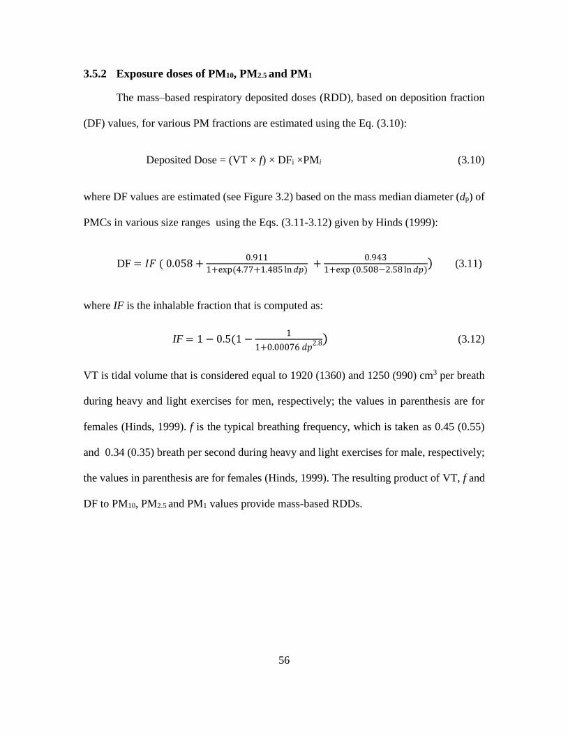
56
3.5.2 Exposure doses of PM10, PM2.5 and PM1
The mass–based respiratory deposited doses (RDD), based on deposition fraction
(DF) values, for various PM fractions are estimated using the Eq. (3.10):
Deposited Dose = (VT × f) × DFi ×PMi (3.10)
where DF values are estimated (see Figure 3.2) based on the mass median diameter (dp) of
PMCs in various size ranges using the Eqs. (3.11-3.12) given by Hinds (1999):
DF = 𝐼𝐹 ( 0.058 +0.911
1+exp (4.77+1.485 ln 𝑑𝑝) +
0.943
1+exp (0.508−2.58 ln 𝑑𝑝)) (3.11)
where IF is the inhalable fraction that is computed as:
IF = 1 − 0.5(1 −1
1+0.00076 𝑑𝑝2.8) (3.12)
VT is tidal volume that is considered equal to 1920 (1360) and 1250 (990) cm3 per breath
during heavy and light exercises for men, respectively; the values in parenthesis are for
females (Hinds, 1999). f is the typical breathing frequency, which is taken as 0.45 (0.55)
and 0.34 (0.35) breath per second during heavy and light exercises for male, respectively;
the values in parenthesis are for females (Hinds, 1999). The resulting product of VT, f and
DF to PM10, PM2.5 and PM1 values provide mass-based RDDs.

57
Figure 3.2: Finding mass median diameter (MMD) of coarse and fine particles using cumulative
particle mass concentrations measured during each activity. DF refers to deposition fraction which
has been estimated using MMD in Eq. (3.11).
0
25
50
75
100
2.5 5.0 7.5 10.0
0
25
50
75
100
0.0 0.6 1.3 1.9 2.5
0
25
50
75
100
0.0 2.5 5.0 7.5 10.0
0
25
50
75
100
0.0 0.6 1.3 1.9 2.5
0
25
50
75
100
0.0 2.5 5.0 7.5 10.00
25
50
75
100
0.0 0.6 1.3 1.9 2.5
0
25
50
75
100
0.0 2.5 5.0 7.5 10.00
25
50
75
100
0.0 0.6 1.3 1.9 2.5
Cum
ula
tive
par
ticl
e m
ass
conce
ntr
atio
ns
of
coar
se a
nd f
ine
par
ticl
es (
%)
0
25
50
75
100
0.0 2.5 5.0 7.5 10.0
Particle size, dp (µg)
0
25
50
75
100
0.0 0.6 1.3 1.9 2.5
50 %
50 %
50 %
50 %
50 %
MMD: 6.00
DF: 0.93
Coarse
particles
Fine
particles
MMD: 1.08
DF: 0.44
MMD: 5.75
DF: 0.93MMD: 1.35
DF: 0.59
MMD: 5.35
DF: 0.94
MMD: 0.75
DF: 0.28
MMD: 5.32
DF: 0.94
MMD: 0.91
DF: 0.37
MMD: 6.50
DF: 0.92MMD: 0.40
DF: 0.14
Fine
particles
Fine
particles
Fine
particles
Fine
particles
Coarse
particles
Coarse
particles
Coarse
particles
Coarse
particles
Fix
ed-s
ite
Mobil
e m
easu
rem
ents
At
dif
fere
nt
dis
tance
sIn
side
the
exca
vat
or
Insi
de
the
off
ice

58
3.6 Chapter summary
This chapter summarises the set of instruments and materials used for measuring
the particle number and mass concentrations, and also presents the methods used to estimate
particle emission factors and occupational exposures. Furthermore, this chapter covers the
physicochemical characterisation of particles using SEM, EDS, XPS and IBA analysis.
This chapter ends by providing descriptions of the instruments used for measuring the
particles, including DMS50, GRIMM (1.107 E), OSIRIS (2315) and TEOM (1400), during
the laboratory, indoor and outdoor field experiments as well as the devices which were
used for measuring meteorological parameters and for recording sampling locations.
Further information about the results of the experiments in the controlled laboratory
environment (i.e. concrete mixing, drilling, cutting), indoor field sites (i.e. building
refurbishment) and outdoor field sites (i.e. construction and demolition) are presented in
Chapters 4, 5, 6 and 7, respectively.
59
Chapter 4. Simulated laboratory investigations
This chapter presents the results of release of ultrafine particles and PM from indoor
simulated building activities (i.e. concrete mixing, drilling and cutting). The chapter also
provides assessments of particles emission factors followed by estimations of exposure
doses.
4.1 Introduction
There have been a number of studies of PMCs of ambient PM10 in urban areas, but
less work has focused on the PM2.5 and PM1 fractions arising from building activities
(Ragheb, 2011) with even less information relating to particles below 100 nm (Kumar et
al., 2013). Whilst research has been undertaken into the effects of ultrafine particles on the
environment and health (Kumar et al., 2011a), there is currently no legal regulation, or
guidelines, for controlling the public exposure to airborne PNCs within the urban
environment, including construction sites (Kumar and Morawska, 2014).
Construction activities such as the mixing, drilling and cutting of concrete have the
potential to generate coarse, fine and ultrafine particles. The manufacture of fresh concrete
typically involves the mixing of coarse and fine aggregates with cement, water and
admixtures in a rotating drum mixer generating considerable airborne dust (Kumar and
Morawska, 2014). Concrete drilling (employing hardened drill bits) is a common activity

60
both at construction sites and within domestic situations and is known to generate coarse
and fine particles (Cook Jr and Harris, 1992). Similarly, the cutting of concrete is common
during refurbishment, maintenance and demolition activities and can also produce coarse
and fine particles. Despite the fact that such activities are undertaken on a daily basis
around the globe, surprisingly little is known about the associated emissions and exposure
levels of the particles produced (Akbar-Khanzadeh and Brillhart, 2002; Broekhuizen et al.,
2011; Kumar et al., 2012b).
Many studies have experimentally measured particle number and size distributions during
manufacturing, handling and usage of engineered nanomaterials (Kumar et al., 2014a,
2010a). For example, PNCs in the 0.06–6.36 ×104 cm−3 range were measured during a
simulated sanding process. Some studies have also measured emissions of nano-sized
particles during different generation methods (Tsai et al., 2012; Tsai et al., 2009), or their
exposure during handling and bagging processes at workplaces (Fujitani et al., 2008; Tsai
et al., 2011). However, most of these studies are related to engineered nanomaterials and
there are hardly many investigations that deal with the construction and demolition
processes.
There are a few studies concerned with PM emissions arising from the drilling and cutting
of materials such as carbon nanofibre as well as composite and silica based nanocomposites
(Sachse et al., 2012), the demolition of structures (Dorevitch et al., 2006), concrete
recycling (2014) and other building and road works (Fuller et al., 2002; Fuller and Green,
2004). A summary of relevant studies is presented in Table 2.1. The importance of particle
emissions from construction sources is likely to increase as the development of urban

61
infrastructure across the globe is expected to reflect world population growth (Kumar et
al., 2012b). In addition, there remain significant uncertainties concerning exposure risk
because the particles characteristics from construction sources may be different from other,
more established sources such as vehicle exhaust (Charron and Harrison, 2003; Kumar et
al., 2010, 2011b) and non-vehicle exhaust sources (Kumar et al., 2013; Voliotis et al.,
2014). Further information about the other sources of PM10, PM2.5, PM1 and ultrafine
particles in the urban environment is described in Section 2.4 (Chapter 2). None of the
studies to date have presented coarse, fine and ultrafine particles emissions and associated
exposure to on-site workers from either of the mixing, drilling or cutting activities (see
Table 2.1), which is the focus of this study.
Taking advantage of research gaps, this work investigates the release of particles in the 5-
10,000 nm range from three (simulated) construction activities (concrete mixing, drilling
and cutting) carried out under controlled conditions in indoor laboratory environment. The
objectives were to analyse the size distributions and proportions of both particle number
and mass concentrations in the studied size range, compute emission factors (EFs) and
exposure to on-site workers.
4.2 Methodology
4.2.1 Experimental setup
Experiments were conducted to measure the release of PM10, PM2.5, PM1 and
ultrafine particles arising from the manufacture of fresh concrete (mixing), and subsequent
processing of hardened concrete by drilling and cutting. The aim of the experiments was
to simulate the activities that occur on typical construction sites and consider the

62
implications for workers who are exposed to such procedures. In addition, using
approaches described in Sections 3.4 and 3.5 in Chapter 3, both the particle number- and
mass-based EFs and occupational exposure doses were estimated for all the four activities
(mixing with GGBS and PFA, drilling and cutting) across the three of the phases described.
A total of four different experiments were performed: (i) concrete mixing with a blended
cement incorporating Portland cement with 35% by weight Ground Granulated
Blastfurnace Slag (GGBS), (ii) concrete mixing with a blended cement incorporating
Portland cement with 35% Pulverised Fuel Ash (PFA), (iii) the drilling of hardened
concrete, and (iv) the cutting of hardened concrete. During each experiment the
measurement of particle emissions was divided into three distinct time periods: (i) the pre-
activity baseline (i.e. background levels in the ambient indoor environment), (ii) the
simulated activity (carried out over a fixed time to enable the EFs and exposure doses to
be estimated), and (iii) the post-activity background level.
The levels of particle emissions arising during each experiment were measured using a
DMS50 and GRIMM instruments (see Section 3.2 in Chapter 3) for measurements of
number and size distributions in the 5-10,000 nm range such that both the particle number
and mass concentrations (PM10, PM2.5, PM1) could be obtained. KESTREL 4500 was also
used for measuring the meteorological data (relative humidity, barometric pressure and
ambient temperature), which was set up next to the DMS50 and GRIMM instruments.
Meteorological information was logged on the Kestrel 4500 during all the experiments
although wind direction and speed were not recorded since all of the measurements
reported here were undertaken in a controlled laboratory environment.

63
Table 4.1: Summary of sampling data during concrete mixing, drilling and cutting activities.
Concrete mixing was carried out using a rotating drum mixer, manufactured by ELE
International (model: EL34-3540/01, Bedfordshire, United Kingdom), with a 100 litre
capacity operating at 60 rpm. Two different concrete mixes were manufactured using the
mix specification shown in Tables A1-A2 (Appendix A) incorporating Portland cement
blended with either GGBS or PFA. Measurements of particle levels were obtained during
the pre-activity and both during the mixing process itself (which took place over a period
of ~180–300 seconds) and subsequently during the measurement of the slump test of the
resulting fresh concrete mix (see Table 4.1). Slump test is used at construction sites to
measure the workability of freshly made wet concrete. This test was carried out following
the method described in BS EN 12350-2. Concrete was filled in a steel slum test cone in
three equal layers to measure the “slump (settlement)” of freshly made concrete after lifting
up the test cone. The test does not involve any mechanical stresses and the probable source
of coarse particles appears to be resuspension of dust from the floor and nano-sized
particles from the chemical reactions undergoing in the fresh mix of concrete.
Date Time Sampling time
(seconds)
Name of activities
03/07/2013 14:40:46
15:27:03
2,777 Mixing with GGBS
04/11/2013 13:28:28
14:39:23
4,255 Mixing with PFA
04/11/2013 14:47:38
15:20:01
1,953 Drilling
04/11/2013 15:21:00
15:41:48
1,248 Cutting
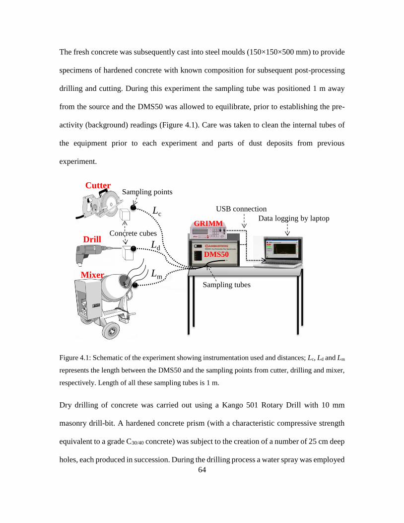
64
The fresh concrete was subsequently cast into steel moulds (150×150×500 mm) to provide
specimens of hardened concrete with known composition for subsequent post-processing
drilling and cutting. During this experiment the sampling tube was positioned 1 m away
from the source and the DMS50 was allowed to equilibrate, prior to establishing the pre-
activity (background) readings (Figure 4.1). Care was taken to clean the internal tubes of
the equipment prior to each experiment and parts of dust deposits from previous
experiment.
Figure 4.1: Schematic of the experiment showing instrumentation used and distances; Lc, Ld and Lm
represents the length between the DMS50 and the sampling points from cutter, drilling and mixer,
respectively. Length of all these sampling tubes is 1 m.
Dry drilling of concrete was carried out using a Kango 501 Rotary Drill with 10 mm
masonry drill-bit. A hardened concrete prism (with a characteristic compressive strength
equivalent to a grade C30/40 concrete) was subject to the creation of a number of 25 cm deep
holes, each produced in succession. During the drilling process a water spray was employed
Mixer
Drill
Cutter
Lc
Ld
Lm
DMS50
Sampling tubes
USB connection
Data logging by laptopGRIMM
Concrete cubes
Sampling points

65
to mimic good construction practice and the sampling tube was positioned at 1 m from the
source in each case (Figure 4.1). Dry cutting was carried out on a hardened concrete prism
(150×150×500 mm) using a Norton BBL527 model, diamond wheel with a blade shaft
speed of 2400 rpm and a 55.88 cm diameter blade of 1.5 mm thickness. Again the sampling
point was 1 m away from source (Figure 4.1).
4.3 Results and discussion
4.3.1 Particle size distributions
The spectrums of particle number distribution (PND) obtained during the simulated
building activities are presented in Figure 4.2a-b (mixing of concrete) and Figure 4.2c-d
(drilling and cutting). It can be seen that during each “activity” period there is a significant
change in the PND over background levels. As expected the post-activity levels are lower
than those obtained during the activity but were somewhat above the original background
reflecting the time taken by particles to disperse after the activity (Section 4.3.2). For
mixing activities undertaken with GGBS and PFA the peak PND values obtained were
2.31×10⁴ and 3.80×104 cm–3 being ~3.0 and 12-times higher than peak background PNDs,
respectively. In terms of nucleation mode particles (those below 30 nm; (Kumar et al.,
2008)) and new particle release, peak PNDs produced during mixing with PFA were ~1.64-
times higher than those obtained with GGBS. This is thought to reflect the particle size,
density and adhesion of the two materials as the mixing process was the same. As seen in
Figure 4.2a-b there is an increase in PNDs in the ultrafine size range during the mixing
process. Figure 4.2c-d show the PND spectrums obtained during the drilling and cutting
of samples of hardened concrete. The peak PND values obtained were 37.10×10⁴ and

66
118.80×104 cm-3, respectively, being ~3.5 and 8-times higher than the background peak
PNDs. A significant increase in nucleation mode particles was observed with cutting
producing a greater release of new particles (over background) than drilling, reflecting the
larger surface area of concrete subject to abrasion. These observations confirm that
significantly more ultrafine particles are released during cutting and drilling activities in
comparison to mixing activities. These results are dissimilar to the findings of Kumar et al.
(2012c), both in terms of peak diameters and the shape of PNDs obtained during their
investigations for estimating the release of particles below 100 nm arising from the
crushing of hardened concrete cubes, the fracture of concrete slabs and the recycling of
concrete debris. For example, their work found peak PNDs at ~20.73×10⁴ and 20.86×10⁴
cm–3 during demolition and dry recycling of concrete, respectively, which is ~2- and ~6-
times larger to that obtained for the drilling and cutting activities reported here.
Figure 4.2: PNDs for the (a) mixing with GGBS and (b) mixing PFA, (c) drilling, and (d) cutting.
104
105
(a)
(b)
(c) (d)
Dp (nm)
dN
/dlo
gD
p(c
m-3
)
0.0
3.0
6.0
9.0
12.0
1 10 100 1000
Background
Drilling activity
Postbackground
0.0
3.0
6.0
9.0
12.0
1 10 100 1000
Background
Cutting
Postbackground
0.0
1.0
2.0
3.0
4.0
1 10 100 1000
Background Mixing with PFA
Slump test Potsbackground
0.0
1.0
2.0
3.0
4.0
1 10 100 1000
Background
Mixing (GGBS)
Slump test
Post background

67
4.3.2 Particle number concentrations
Figure 4.3 and Figure 4.4 show the total PNCs and distribution of particles in
various size ranges obtained during mixing (with GGBS and PFA), drilling and cutting,
respectively. Average PNCs during the activity periods in size ranges 5-30, 30-100, 100-
300 and 300-560 nm were 21.27±2.02 ×10³, 30.97±16.51 ×10³, 279.11±61.92 ×10³ and
732.27±442.51 ×103 cm-3 for mixing with GGBS, PFA, drilling and cutting, respectively.
Average PNC values during mixing with GGBS and PFA were ~4 and 15-times above the
background levels, Table 4.2.
Table 4.2: Average concentration, Geometrical mean diameter and fractions for particles number
during mixing, drilling and cutting activities.
Experiments Time period Average ± STD
(# cm-3) ×103
Geometrical
mean diameter
Ultrafine
particles fraction
(%)
Mixing with
GGBS
Background 5.26±1.24 58.96±2.56 68
Mixing with GGBS 21.72±2.02 53.01±2.50 74
Slump test 11.12±6.10 35.95±3.23 78
Post background 11.88 ±2.25 67.49±2.36 65
Mixing with
PFA
Background 1.98±1.42 63.15±2.39 66
Mixing with fly ah 30.97±16.61 41.93±2.28 82
Slump test 8.61±6.09 34.97±2.15 88
Post background 4.08±1.67 4.08±1.67 80
Drilling Background 69.85±7.15 30.90±2.34 90
Drilling 279.11±61.92 19.55±2.50 95
Post background 146.64±24.35 26.41±2.33 94
Cutting Background 127.32±16.65 27.68±2.28 93
Cutting 732.27±442.51 15.10±2.17 97
Post background 233.64±133.57 23.23±2.40 93

68
Figure 4.3: Temporal evolution of PNC and their contour plots during (a) mixing with GGBS, and
(b) mixing with PFA.
0.0
0.4
0.8
1.2
1.6
14:44:06 14:51:18 14:58:30 15:05:42 15:12:54 15:20:06
PN
C (
#cm
-3)
Time(s)
Background
Mixing
with GGBS
Slump test
Post background
510
20
50
100
200
500
14:44:06 14:51:18 14:58:30 15:05:42 15:12:54 15:20:06
Par
ticl
e dia
met
er (
nm
)
105
1.E+3 6.3E+3 4.E+4 2.5E+5 1.6E+6 1.E+7
dN/dlogdp /cc
0.0
0.4
0.8
1.2
1.6
13:46:34 13:59:31 14:12:29 14:25:26 14:38:24
Background Slump test Post-backgroundMixing with PFA
510
50
100
200
500
13:46:33 14:00:57 14:15:21 14:29:45
20
PN
C (
#cm
-3)
Par
ticl
e dia
met
er (
nm
) 1.E+3 6.3E+3 4.E+4 2.5E+5 1.6E+6 1.E+7
dN/dlogdp /cc
105
Time(s)
(a)
(b)

69
The average PNCs during the drilling activity changed relatively little. For example, these
were ~1.38-times higher for the second hole than during the first hole (Figure 4.4a).
Average values over the period of drilling periods were ~ 4–times higher than background
level (69.85±7.15 ×103 cm-3), as seen in Table 4.2. For all the activities, the ultrafine size
range (below 100 nm) contributed most of the total PNCs. For example, their proportion to
total PNCs during the mixing with GGBS, mixing with PFA, drilling and cutting activities
was 74, 82, 95 and 97%, respectively (see Figure A1 in Appendix A). The peak value for
the “dry” drilling activity was 5.14 105 cm-3 and decreased by ~40% to 3.08×105 cm-3 when
water spraying was employed as a suppression method since particles are less able to
become airborne (Rosenfeld et al., 2001).
The average PNC measured during concrete cutting was 732.27±442.51 ×103 cm-3, which
is ~14–times greater than the background value, Table 4.2. Taken together Figure 4.3 and
Figure 4.4 demonstrate that for both the drilling and cutting activities there is an increase
in PNC with time and the magnitude of PNC are much higher than occurred during the
mixing of fresh concrete. This is thought to reflect the higher rotational frequency, shear
stresses and local energy density associated with drilling and cutting activities. Again these
results are in agreement with those of Kumar et al. (2012c) who reported an increase of
between 2– and 17–times in the total PNC over the background PNCs for various concrete
demolition related activities. After adjusting for background concentrations, the net release
of PNCs during cube crushing and ‘dry’ recycling of concrete events were measured as
~0.77 and 22.70 (×104) cm−3, respectively. The corresponding results reported by Kumar
et al. (2012c) were about (2.76, 0.09), (4.02, 0.13), (36.23, 1.22) and (95.06, 3.22) times

70
smaller than values for mixing with GGBS, with PFA, drilling and cutting activities,
respectively.
Figure 4.4: Temporal evolution of PNC and their contour plots during (a) drilling, and (b) cutting
activities.
0.0
0.5
1.0
1.5
2.0
2.5
14:57:24 15:04:36 15:11:48 15:19:00
Mil
lio
ns
Background Post- background
1st hole
2nd hole
3rd hole
5
10
20
50
100
200500
14:57:24 15:04:36 15:11:48 15:19:00
106
1.E+3 6.3E+3 4.E+4 2.5E+5 1.6E+6 1.E+7
dN/dlogdp /cc
PN
C (
#cm
-3)
Par
ticl
e dia
met
er (
nm
)
Time(s)
0.0
0.5
1.0
1.5
2.0
2.5
15:13:13 15:20:25 15:27:37 15:34:49 15:42:01
Background Cutting Post-background
Time(s)
5
10
20
50
100
200
500
15:13:33 15:20:45 15:27:57 15:35:09
106
PN
C (
#cm
-3)
Par
ticl
e d
iam
eter
(n
m)
1.E+3 6.3E+3 4.E+4 2.5E+5 1.6E+6 1.E+7
dN/dlogdp /cc
(b)
(a)

71
The values of PNC obtained during these processes are not directly comparable but can be
put in perspective of the average roadside and urban background PNCs. The corresponding
values of PNCs in European environments were reported as 3.15±1.60 ×104 cm–3 and
1.63±0.82 ×104 cm–3, respectively (Kumar and Morawska, 2013; Kumar et al., 2014),
indicating that studied activities may produce particles at levels (above background) that
are comparable to, or greater than, those which arise from vehicle exhausts. Given that
construction and demolition activities occur within urban areas this raises important
questions about the need to understand the associated exposure levels to urban dwellers,
building operatives and the need to establish suitable standards and controls.
4.3.3 Particle mass concentrations
Figure 4.5 shows the PMC arising from the mixing of concrete with GGBS and
PFA. The average PM10, PM2.5 and PM1 determined during mixing were 1.89×10³,
0.78×10³, 0.56×10³ µg m-3 and 1.98×10³, 0.94×10³, 0.63×10³ µg m-3, respectively (see
Figure A2 in Appendix A). PMC values showed a rapid increase immediately after the start
of mixing. The peak values of PM10, PM2.5 and PM1 reached 4.10×10³, 3.65×10³ and
2.42×10³ µg m-3 for the concrete containing GGBS. The corresponding values obtained for
the mix containing PFA were 3.66×10³, 2.35×10³ and 1.04 ×10³ µg m-3, which are many
times higher than those for the mixing with the GGBS reflecting the same trend as seen for
the PNCs (see Section 4.3.2). The results of the drilling and cutting activities show a
considerable increase in PMC over background levels. Moreover, the average PM10, PM2.5
and PM1 were calculated as 2.82×10³, 1.19×10³, 0.80×10³ µg m-3 for drilling and 3.77×10³,
1.34×10³, 0.86×10³ µg m-3 for cutting, Table 4.3.

72
Figure 4.5: Mass concentration against time for (a) mixing with GGBS, (b) mixing with PFA, (c)
drilling, and (d) cutting activities.
BackgroundMixing
with GGBS Slump test Post-background
PM
1(µ
g m
-3)
PM
10;
PM
2.5
(µgm
-3)
0.0
0.7
1.4
2.1
2.8
0.0
2.0
4.0
6.0
8.0
14:4
4:1
3
14:4
6:0
7
14:4
8:0
1
14:4
9:5
5
14:5
1:4
9
14:5
3:4
3
14:5
5:3
7
14:5
7:3
1
14:5
9:2
5
15:0
1:1
9
15:0
3:1
3
15:0
5:0
7
15:0
7:0
1
15:0
8:5
5
15:1
0:4
9
15:1
2:4
3
15:1
4:3
7
15:1
6:3
1
15:1
8:2
5
15:2
0:1
9
15:2
2:1
3
15:2
4:0
7
15:2
6:0
1
PM10
PM2.5
PM1
103
BackgroundMixing
with PFASlump test Post background
PM
1(µ
g m
-3)
PM
10;
PM
2.5
(µg m
-3)
103
0.0
0.7
1.4
2.1
2.8
0.0
2.0
4.0
6.0
8.0
13
:48
:01
13
:50
:25
13
:52
:49
13
:55
:13
13
:57
:37
14
:00
:01
14
:02
:25
14
:04
:49
14
:07
:13
14
:09
:37
14
:12
:01
14
:14
:25
14
:16
:49
14
:19
:13
14
:21
:37
14
:24
:01
14
:26
:25
14
:28
:49
14
:31
:13
14
:33
:37
14
:36
:01
14
:38
:25
PM10
PM2.5
PM1
USED
Background
Drilling Post background
PM
1(µ
g m
-3)
PM
10;
PM
2.5
(µgm
-3)
0.0
0.7
1.4
2.1
2.8
0.0
2.0
4.0
6.0
8.0
14
:57
:00
14
:58
:12
14
:59
:24
15:0
0:3
6
15:0
1:4
8
15:0
3:0
0
15:0
4:1
2
15
:05
:24
15
:06
:36
15
:07
:48
15
:09
:00
15
:10
:12
15
:11
:24
15
:12
:36
15
:13
:48
15
:15
:00
15
:16
:12
15
:17
:24
15
:18
:36
15
:19
:48
PM10
PM2.5
PM1
103
Background Cutting Post background
PM
1(µ
gm
-3)
PM
10;
PM
2.5
(µgm
-3)
0.0
0.7
1.4
2.1
2.8
0.0
2.0
4.0
6.0
8.0
15
:13
:00
15
:14
:24
15
:15
:48
15
:17
:12
15
:18
:36
15
:20
:00
15
:21
:24
15
:22
:48
15
:24
:12
15
:25
:36
15
:27
:00
15
:28
:24
15
:29
:48
15
:31
:12
15
:32
:36
15
:34
:00
15
:35
:24
15
:36
:48
15
:38
:12
15
:39
:36
15
:41
:00
PM10
PM2.5
PM1
103
USED
(a)
(b)
(c)
(d)
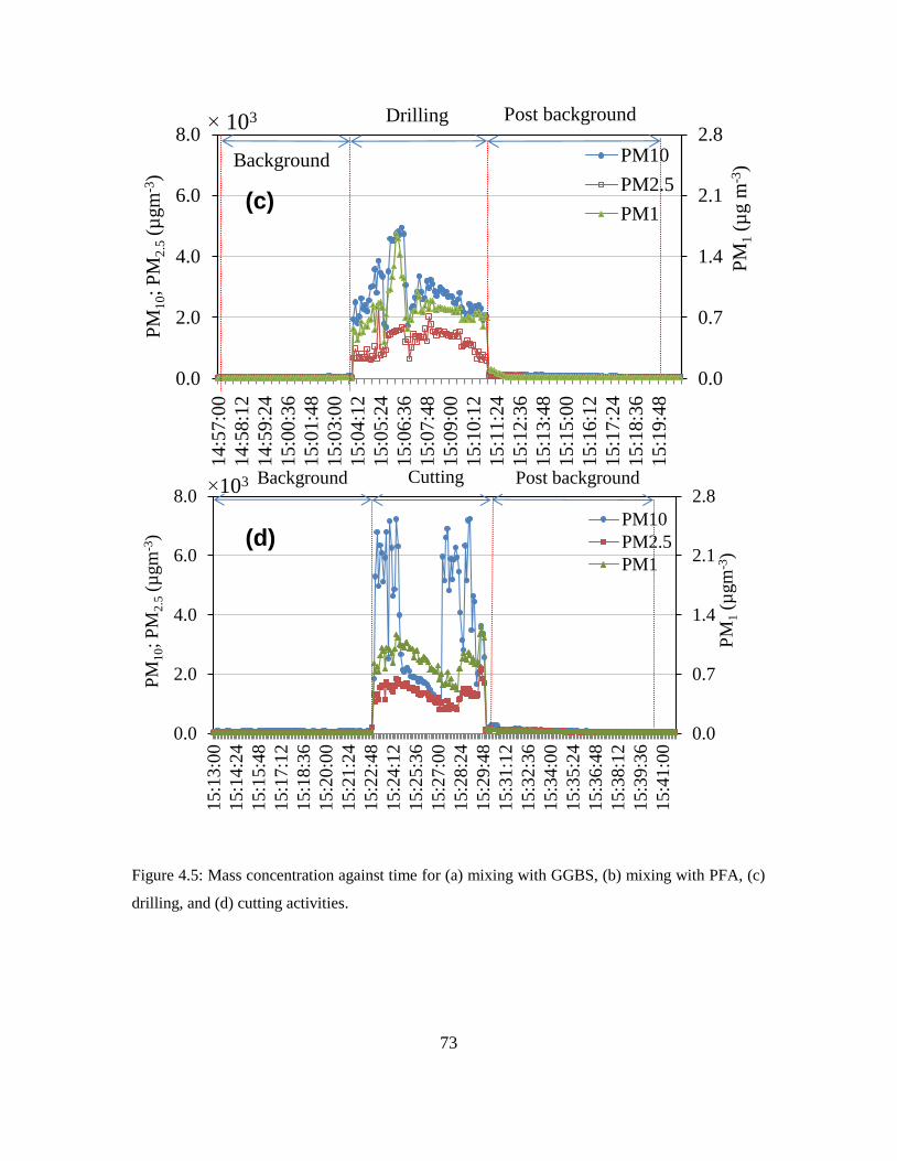
73
Figure 4.5: Mass concentration against time for (a) mixing with GGBS, (b) mixing with PFA, (c)
drilling, and (d) cutting activities.
BackgroundMixing
with GGBS Slump test Post-background
PM
1(µ
g m
-3)
PM
10;
PM
2.5
(µgm
-3)
0.0
0.7
1.4
2.1
2.8
0.0
2.0
4.0
6.0
8.0
14:4
4:1
3
14:4
6:0
7
14:4
8:0
1
14:4
9:5
5
14:5
1:4
9
14:5
3:4
3
14:5
5:3
7
14:5
7:3
1
14:5
9:2
5
15:0
1:1
9
15:0
3:1
3
15:0
5:0
7
15:0
7:0
1
15:0
8:5
5
15:1
0:4
9
15:1
2:4
3
15:1
4:3
7
15:1
6:3
1
15:1
8:2
5
15:2
0:1
9
15:2
2:1
3
15:2
4:0
7
15:2
6:0
1
PM10
PM2.5
PM1
103
BackgroundMixing
with PFASlump test Post background
PM
1(µ
g m
-3)
PM
10;
PM
2.5
(µg m
-3)
103
0.0
0.7
1.4
2.1
2.8
0.0
2.0
4.0
6.0
8.0
13
:48
:01
13
:50
:25
13
:52
:49
13
:55
:13
13
:57
:37
14
:00
:01
14
:02
:25
14
:04
:49
14
:07
:13
14
:09
:37
14
:12
:01
14
:14
:25
14
:16
:49
14
:19
:13
14
:21
:37
14
:24
:01
14
:26
:25
14
:28
:49
14
:31
:13
14
:33
:37
14
:36
:01
14
:38
:25
PM10
PM2.5
PM1
USED
Background
Drilling Post background
PM
1(µ
g m
-3)
PM
10;
PM
2.5
(µgm
-3)
0.0
0.7
1.4
2.1
2.8
0.0
2.0
4.0
6.0
8.0
14:5
7:0
0
14:5
8:1
2
14:5
9:2
4
15
:00
:36
15
:01
:48
15
:03
:00
15
:04
:12
15:0
5:2
4
15:0
6:3
6
15:0
7:4
8
15:0
9:0
0
15:1
0:1
2
15:1
1:2
4
15:1
2:3
6
15:1
3:4
8
15:1
5:0
0
15:1
6:1
2
15:1
7:2
4
15:1
8:3
6
15:1
9:4
8
PM10
PM2.5
PM1
103
Background Cutting Post background
PM
1(µ
gm
-3)
PM
10;
PM
2.5
(µgm
-3)
0.0
0.7
1.4
2.1
2.8
0.0
2.0
4.0
6.0
8.0
15
:13
:00
15
:14
:24
15
:15
:48
15
:17
:12
15
:18
:36
15
:20
:00
15
:21
:24
15
:22
:48
15
:24
:12
15
:25
:36
15
:27
:00
15
:28
:24
15
:29
:48
15
:31
:12
15
:32
:36
15
:34
:00
15
:35
:24
15
:36
:48
15
:38
:12
15
:39
:36
15
:41
:00
PM10
PM2.5
PM1
103
USED
(a)
(b)
(c)
(d)

74
The peak PMC values of PM10, PM2.5 and PM1 during drilling were 4.94×10³, 2.38×10³
and 1.65×10³ µg m-3, which are higher than the values of 7.21×10³, 2.05×10³ and 1.26×10³
µg m-3 for the cutting activity. This substantiates the fact that the cutting activity not only
produces more particles, by number (Section 4.3.2) but also greater particle mass emissions
compared with the drilling activity.
Overall, the results in Figure 4.5 show an increase in the average PMC over background
levels during the various activities reflecting the release of new particles. PM10, PM2.5 and
PM1 are 32, 58 and 86 times the background during the mixing of concrete with GGBS and
32, 50, 89 times when mixing concrete with PFA. In the same way PM10, PM2.5 and PM1
for the drilling activity were 45, 80 and 115 times the background during the drilling
activity, and 50, 80 and 122 times higher during the cutting activity. Depending on the
source the values of PMCs varied, however, in all cases the PMC values increased with
increasing PNCs (see Section A1 in Appendix A).
It is interesting to compare these results with the work of Hansen et al. (2008) who carried
out environmental sampling of PM during demolition of a hospital building. They found a
2.9-times increase in concentration for particles higher than 0.5 μm and 3.3-times for
particles about 1 μm. This increase was less marked than that of demolition by implosion
(Dorevitch et al., 2006) which has been shown to be associated with short-term
concentrations of PM, 10-times higher than pre-implosion levels.

75
Table 4.3: The concentrations of PM10, PM2.5 and PM1 during the activity period. STD and
percentage fraction (PF) represent standard deviation and particles fraction of mixing with GGBS,
PFA, drilling and cutting, respectively.
Activities PM10
Avg ± STD (µg m-3)
PM2.5
Avg ± STD (µg m-3)
PM1
Avg ± STD (µg m-3)
Mixing with
GGBS
Background 58.45±9.19 13.37±5.46 6.52±0.65
Mixing with GGBS 1891.28±1212.20 780.65±769.99 562.23±541.26
Slump test 736.12±416.50 366.44 ±165.26 278.27±40.13
Post background 73.70 ±60.84 59.96 ±25.43 17.76±3.80
Mixing with
PFA
Background 61.60±8.41 18.71 ±14.88 7.14±1.99
Mixing with PFA 1986.12±824.44 945.30±405.7 636.61±48.21
Slump test 846.44±335.68 409.71±402.17 353.67±269.35
Post background 79.63±48.70 62.63±28.71 18.52±2.16
Drilling Background 63.40±7.47 14.98±3.17 6.95±2.42
Drilling 2827.27±820.99 1193.41±391.18 801.49± 228.81
Post background 86.74±25.56 61.25±13.72 18.87±18.72
Cutting Background 74.50±13.547 16.76±18.77 7.12±2.55
Cutting 3777.18±2065.46 1345.85±310.474 867.75±172.37
Post background 89.03±50.42 61.12±28.65 21.95±7.87
4.3.4 Emission factors
EFs for any activity are calculated in accordance with method described in Section
3.4.1. It was made to identify the number and mass of particles being released from the
source and to indicate how many particles can be inhaled by an occupant during the
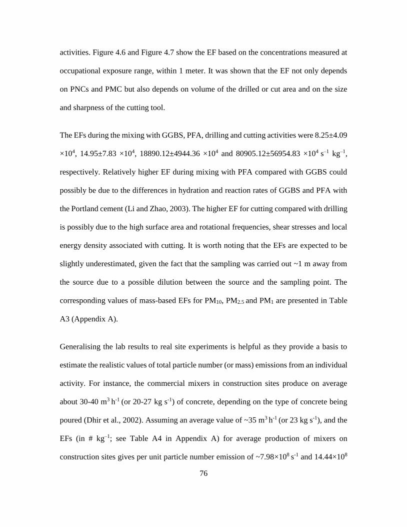
76
activities. Figure 4.6 and Figure 4.7 show the EF based on the concentrations measured at
occupational exposure range, within 1 meter. It was shown that the EF not only depends
on PNCs and PMC but also depends on volume of the drilled or cut area and on the size
and sharpness of the cutting tool.
The EFs during the mixing with GGBS, PFA, drilling and cutting activities were 8.25±4.09
×104, 14.95±7.83 ×10⁴, 18890.12±4944.36 ×104 and 80905.12±56954.83 ×104 s–1 kg–1,
respectively. Relatively higher EF during mixing with PFA compared with GGBS could
possibly be due to the differences in hydration and reaction rates of GGBS and PFA with
the Portland cement (Li and Zhao, 2003). The higher EF for cutting compared with drilling
is possibly due to the high surface area and rotational frequencies, shear stresses and local
energy density associated with cutting. It is worth noting that the EFs are expected to be
slightly underestimated, given the fact that the sampling was carried out ~1 m away from
the source due to a possible dilution between the source and the sampling point. The
corresponding values of mass-based EFs for PM10, PM2.5 and PM1 are presented in Table
A3 (Appendix A).
Generalising the lab results to real site experiments is helpful as they provide a basis to
estimate the realistic values of total particle number (or mass) emissions from an individual
activity. For instance, the commercial mixers in construction sites produce on average
about 30-40 m3 h-1 (or 20-27 kg s-1) of concrete, depending on the type of concrete being
poured (Dhir et al., 2002). Assuming an average value of ~35 m3 h-1 (or 23 kg s-1), and the
EFs (in # kg–1; see Table A4 in Appendix A) for average production of mixers on
construction sites gives per unit particle number emission of ~7.98×10⁸ s-1 and 14.44×10⁸

77
s-1 during mixing with GGBS and PFA, respectively. Similar estimates can be made for the
cutting and drilling activities in order to assess the extent of total particle number emissions
from these activities.
Figure 4.6: Particle number concentration based EFs for all the four activities. Please note that these
are net EFs estimated using the net sum of PNCs (i.e. total during the activity period minus the
background PNCs during pre-activity period).
(a) (b)
(d)(c)
0
2
4
6
8
10
#/sec #/sec.kg #/kg
Mixing with GGBS
107
# s–1 # s–1 kg–1 # kg–1
0
2
4
6
8
10
#/sec #/sec.kg #/kg
Mixing with PFA
107
# s–1 # s–1 kg–1 # kg–1
0
4
8
12
16
#/sec #/sec.kg #/kg
Drilling
109
# s–1 # s–1 kg–1 # kg–10
23
45
68
90
#/sec #/sec.kg #/kg
Cutting
109
# s–1 # s–1 kg–1 # kg–1
0.00
0.10
0.20
#/sec #/sec.kg
107
# s–1 # s–1 kg–1 0.0
0.1
0.2
0.3
0.4
0.5
#/sec #/sec.kg
107
# s–1 # s–1 kg–1
0.0
0.1
0.2
0.3
#/sec #/sec.kg
109
# s–1 # s–1 kg–1 0.0
0.3
0.6
0.9
1.2
1.5
#/sec #/sec.kg
109
# s–1 # s–1 kg–1
Em
issi
on f
acto
rs (
# s–
1;
# s–
1 k
g–
1;
# k
g–
1)

78
Figure 4.7: Particle mass concentration based EFs for all the four activities. Please note that these
are net EFs estimated using the net sum of PMCs (i.e. total during the activity period minus the
background PMCs during pre-activity period).
4.3.5 Exposure assessment
Measuring the occupational exposure to ultrafine particles and PM at construction
sites is subject to several factors, which influence the level of particles exposure. The first
is the size range of the measured particles and their concentration. The average dose rates
0.0
0.2
0.4
0.6
0.8
Mixing
with
GGBS
Mixing
with
PFA
DrillingCutting
0.0
0.1
0.2
0.3
0.4
Mixing
with
GGBS
Mixing
with
PFA
Drilling Cutting
0.0
0.4
0.8
1.2
1.6
Mixing
with
GGBS
Mixing
with
PFA
Drilling Cutting
0.0
0.1
0.2
0.3
0.4
Mixing
with
GGBS
Mixing
with
PFA
Drilling Cutting
0.0
0.1
0.2
0.3
0.4
Mixing
with
GGBS
Mixing
with
PFA
Drilling Cutting
0.00
0.01
0.02
0.03
0.04
Mixing
with
GGBS
Mixing
with
PFA
Drilling Cutting
0.00
0.04
0.08
0.12
0.16
Mixing
with
GGBS
Mixing
with
PFA
Drilling Cutting
Hu
nd
red
s
0.00
0.10
0.20
0.30
0.40
Mixing
with
GGBS
Mixing
with
PFA
Drilling Cutting
PM
(µ
g s
–1)
PM
(µ
g k
g–
1)
PM
(µ
g s
–1
kg–
1)
x100 x100 x100
x102 x102 x102
x100 x100x100
PM10 PM2.5 PM1
PM10 PM2.5 PM1
PM2.5 PM1PM10
0.0
0.3
0.5
0.8
1.0
Mixing
with
GGBS
Mixing
with
PFA
Drilling Cutting

79
over the activities for particle numbers were estimated using (i) constant DF, and (ii) size-
dependant DFs and (as described in Section 3.5). The approach (ii) provided the total
deposited doses as 2.35±0.31 ×10⁸ min−1, 3.40±2.17 ×10⁸ min−1, 32.97±9.41 ×10⁸ min−1
and 88.25±58.82 ×10⁸ min−1 for mixing with GGBS, with PFA, drilling and cutting,
respectively (see Table A5 in Appendix A). Figure 4.8 shows the overall differences
between the two approaches. In general, exposure studies using constant DF values can
provide a satisfactory approximation of the dose inhaled by commuters. However, an
underestimation of dose can be seen for cases in which the vast majority of inhaled particles
are in the nucleation mode (i.e. those below 30 nm in diameter).
Figure 4.8: Respiratory tract deposition dose rate (# min−1) calculated using (i) size-dependent DFs
and average size-resolved PNCs, and (ii) a constant DF and the average PNC for each activity.
0
3
6
9
12
15
1 2 3 4
109
Mixing
with
GGBS
Mixing
with PFADrilling Cutting
Res
pir
ato
ry d
epo
siti
on
do
ses
(# m
in-1
)
0.0
0.2
0.4
0.6
1 2Mixing
with
GGBS
Mixing
with PFA
109
0.0
3.0
6.0
9.0
12.0
15.0
1 2 3 4
Dose calculated by variable DF and concentrations classified by partcile size
Dose Calculated by fixed DF and averaged total concentration
109
Dose with variable DF
Dose with constant DF
80
There is currently no data available for direct comparison of results of this study with other
exposure studies. Therefore the closest possible exposure studies have been picked for this
purpose. For example, Kumar and Morawska (2014) reported results on exposure to
airborne particles during simulated concrete recycling activity. The deposited fraction of
total PNCs were found to be 24.83×10⁸ min–1 during exposure close to the source. The
deposited fraction for mixing with GGBS, with PFA, drilling and cutting was found to be
~0.09, 0.13, 1.32, and 3.55 times higher, respectively, compared with those obtained by
Kumar and Morawska (2014) for concrete recycling. Urban exposure study of Joodatnia et
al. (2013a) estimated the average dose rates over the 30 car journeys in Guildford (UK)
using used size-dependant DFs as 5.50±5.09 ×10⁸ min−1. These come out ~0.43, 0.62, 5.99
and 16.05 times smaller than those for mixing with GGBS, with PFA, drilling and cutting,
respectively. Similarly, Int Panis et al. (2010) calculated the dose rate for cycling and car
journeys in Brussels (Belgium) by applying a constant DF (0.63) as 9.02×10⁸ min-1 and
1.49×10⁸ min-1, respectively. These are about (0.26, 1.58), (0.38, 2.28), (3.66, 22.12) and
(9.78, 59.22) times smaller than those for mixing with GGBS, with PFA, drilling and
cutting, respectively.
4.4 Chapter summary and conclusions
A DMS50 and GRIMM were used to measure particle number and size distributions
in the 5–10,000 nm size range of particles released by mixing, drilling and cutting activities.
The objectives were to understand the number and mass emission characteristics of
particles in various size ranges during these simulated building activities, along with

81
estimating the emission factors and exposure of site workers to ultrafine particles and PM
from these activities.
The cutting was found to produce the highest release of new particles in terms of both
PNCs and PNDs, followed by the drilling and mixing activities. Overall, the results
confirm that the simulated building activities studied here have the potential to release
ultrafine particles at levels above that encountered in the normal background. The use
of water sprays as a controlling measure worked well to suppress associated dust
release.
Ultrafine particles were found to dominate the total PNCs with 74, 83, 95 and 97%
during the mixing (with GGBS and PFA), drilling and cutting activities respectively,
with the highest proportion of ultrafine particles arising from the cutting of concrete.
Particles number distributions were dominated by the 5-100 size range during the both
drilling and cutting activities.
The net average PNC after subtracting the background from the PNCs during the
mixing with GGBS, PFA, drilling and cutting activities were found to be 1.60, 2.89,
20.92 and 60.49 10
4 cm
-3, respectively, showing up 38-times higher values of average
PNCs for cutting activity compared with those for mixing with the GGBS.
The results demonstrate the highest proportion of the total PMCs for coarse particles
with 52% during mixing with PFA, and 58, 59 and 64% for the drilling, mixing with
GGBS and cutting activities, respectively.
The average mass concentration of PM2.5 and PM1 during mixing with GGBS, PFA,
drilling and cutting were measured as (780.65, 562.23), (945.30, 636.61), (1193.41,
82
801.49) and (1345.85, 867.75) µg m-3, which shows many times higher values for
cutting, and drilling than mixing activities.
Particle number based emission rates were estimated as 173.41±8.43 ×10⁴,
314.01±164.55 ×10⁴, 2266.81±593.32 ×10⁴ and 6553.34±4613.34 ×104 s-1 for mixing
with GGBS, PFA, drilling and cutting, respectively, which are much lower than the
emission rate obtained from floor sweeping activity as 2×10⁹ s-1 (He et al., 2004).
This study has presented hitherto missing information concerning the potential for
concrete mixing, drilling and cutting activities to produce ultrafine particles in significant
quantities. This has implications both for the owners of buildings and structures and
regulatory bodies, who appear to be unaware of the potential for building works to give
rise to ultrafine particles at levels significantly above typical background exposures.
Further work now needs to be carried out to compare the results of these laboratory based
studies with data from real indoor and outdoor field sites and establish the exposure levels
that can occur for those carrying out such activities, and those that live or work adjacent
to such sites. For this purpose, the measurements of particles during indoor field activities
(i.e. building refurbishment activities) were carried out and the results are presented in
Chapter 5.

83
Chapter 5. Indoor building refurbishment activities
This chapter presents the results of measurements of PM and ultrafine particles
measurements, taken during the indoor building refurbishment activities (e.g.
welding, wall chasing, sanding and crushing) at an operational refurbishment site.
The chapter also provides information on morphology and composition of the
particles through SEM, XPS and IBA analysis followed by occupation exposure
assessments.
5.1 Introduction
The principles of sustainable urban development are well established, but the extent
of pollution due to refurbishment activities is still unknown. The aim of building
refurbishment is typically to adapt the existing space to meet the needs and expectations of
occupants and bring older buildings up to modern standards for heating, lighting and energy
efficiency, as well as to give outdated buildings an upgrading and redesign that goes beyond
the cosmetic. The drive for sustainable refurbishment includes both the provision of
improved lighting, insulation, ventilation and facilities to ensure the comfort and needs of
users as well as related measures to reduce energy consumption in buildings (Mickaityte et
al., 2008; Omer, 2008; Sunikka and Boon, 2003).

84
Within many existing urban environments, refurbishment has become a major, and
increasingly important, activity and it is predicted to become the dominant construction
activity in the years ahead (Sartori et al., 2008). Due to the increase in rate of population
within urban areas (Egbu, 1999; Kumar et al., 2013a), activities related to refurbishment of
the building stock as a percentage of all building work have already grown in most
European countries over the last 20 years (Kohler and Hassler, 2002). Refurbishment
activities are expected to grow further as more than 60% of the world’s population are
likely to be living in urban areas by 2035 (GroBmann et al., 2013). Such long-term changes
in building demand within Europe will constrain the building professions to shift their
focus from new construction to the maintenance and refurbishment of existing buildings
(Kohler and Hassler, 2002).
In recognition of changes in the age of structure and population rate within urban
environments, significant sectors of the construction industry have concentrated on
developing innovative refurbishment techniques. However, the various demolition and
construction activities associated with building refurbishment are known to produce
copious PM, including coarse, fine and ultrafine particles (Kumar et al., 2012b, 2013b).
PM has serious environmental and health-related consequences because it contains a wide
variety of toxic organic and metallic compounds (Heal et al., 2012). Urban dust,
particularly PM10, is harmful since it can be easily introduced in the respiratory system
(Davila et al., 2006), although there is increasing interest in PM2.5 and ultrafine particles
since these penetrate deeper into the lungs and are thought to be of greater concern for
human health (Chaloulakou et al., 2003). Building activities produce both airborne dust

85
(Batonneau et al., 2004) and the emissions of ultrafine particles (Azarmi et al., 2014;
Kumar and Morawska, 2014) which are causally involved in greater inflammatory
responses than the coarse particles per given mass (HEI, 2013; Kumar et al., 2014).
Refurbishment activities are important part of building construction since these can have
an associated carbon footprint of the order of 20% of the emissions that arise from the
original construction (Pacca and Horvath, 2002). Therefore, the development of efficient
monitoring strategies to study the concentration and distribution of urban particles can help
in mitigating the effects of urban pollution on public health. As a consequence, it is
essential to determine the exposure levels of operatives involved in building refurbishment
as well as understanding the distribution and propagation of particulate materials into the
surrounding environment.
As described in Section 2.4 (Chapter 2) it has now been established that various size of
particles arising from vehicle exhaust and non-vehicle exhaust sources enhance their
concentrations in certain areas (Dall’Osto et al., 2011; Hopke et al., 1980; Kumar and
Morawska, 2014; Kumar et al., 2010, 2011b, 2013b). A few studies have also reported the
particle number and mass emissions arising from the demolition of buildings and transport
structures (Dorevitch et al., 2006; Hansen et al., 2008), concrete recycling (Kumar and
Morawska, 2014) and road works (Fuller et al., 2002; Fuller and Green, 2004). Several
studies have also analysed the composition of particles derived from such sources and a
number of attempts have been made to relate the observed elemental concentrations in
collected particle samples to such activities (Adachi and Tainosho, 2004; Adhami et al.,
2012; Adhami et al., 2014; Batonneau et al., 2004; Chen et al., 2000; Mouzourides et al.,
86
2015; Pattanaik et al., 2012). Further information about the SEM, XPS and IBA analysis
of the particles is presented in Section 2.6 (Chapter 2).
Over the past 35 years, there has been ~20% increase in refurbishment work in relation to
the total volume of UK construction output (Egbu, 1999). This study investigates the
release of particle number distribution (PNDs) and concentrations (PNCs) in sub-
micrometre range, along with PMCs in PM10, PM2.5 and PM1 size range, arising from a
number of refurbishment activities and associated occupational exposure for construction
workers. The characteristics of these particles have also been investigated to help
understand their physicochemical nature and the potential impact of associated exposure
on operatives undertaking building refurbishment.
5.2 Materials and methods
5.2.1 Site description and sampling setup
Experiments were carried out at an indoor refurbishment site (Chemistry
Laboratory) at the University of Surrey that was 31 m long and 15.5 m wide to measure
the PM10, PM2.5, PM1 and ultrafine particles released from refurbishment activities
(Figure 5.1). The data were collected for a total of 55 working hours between 08:00 and
18:00 h (local time) over a period of 8 days; of which, one day was without any activity
that enabled us to evaluate the levels of local background (Figure 5.2).
The refurbishment site had 1 m wide and 0.32 m deep windows that were slightly open
most of the sampling duration (Figure 5.2). However, the ambient wind speed during the
sampling period was relatively low (<1.5 m s–1), giving almost steady dilution conditions
at the site during the study period. There were also three door openings towards a main

87
corridor (Figure 5.2) but these doors were covered with a thick plastic sheet acting as a
temporary protection shield for trapping the particles released on the site. Further details
of the description of site can be seen in Section B1, Appendix B.
Figure 5.1: Schematic diagram of the experimental set-up, showing instrumentation used and
sampling locations.
An exhaustive list of a number of refurbishment activities performed during the sampling
period is presented in Table B1 in Appendix B. Over 20 different refurbishment activities
were counted, including some of the most frequent ones such as general demolition and
cutting of concrete, welding, wall chasing, painting, cutting abrasive blasting, hammering,
impact driving, sawing and cementing (Table B1 and Figure B1). Emitted particles were
measured in the 5-10,000 nm size range using a GRIMM particle spectrometer (model
1.107 E) and a DMS50, as described in Section 3.2 (Chapter 3). The time stamp of both
the instruments was set same to local GMT time. The instrument was placed at the closest
safe place (~2 m from the closest activity) at the site (Figure 5.2). Five different samples
were also collected on Polytetrafluoroethylene (PTFE) filters by the GRIMM instrument
Sampling point
31 m
15
.5 m
Main doorDoor Door
Data logging by laptop
DMS50
GRIMM
KESTREL
4500
Sampling tubes3 m1.5 m 1.5 m
1 m 1 m 1 m
Window
Window
Room 2Room 1
Main Hall
1 m
1 m
1 m
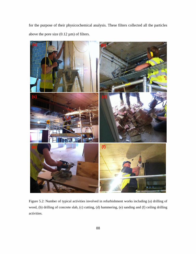
88
for the purpose of their physicochemical analysis. These filters collected all the particles
above the pore size (0.12 µm) of filters.
Figure 5.2: Number of typical activities involved in refurbishment works including (a) drilling of
wood, (b) drilling of concrete slab, (c) cutting, (d) hammering, (e) sanding and (f) ceiling drilling
activities.
(a) (b)
(c) (d)
(e) (f)

89
5.2.2 Collection of PM mass on PTFE filters for SEM, IBA and XPS analysis
Five samples, namely samples 1-5, were collected on PTFE filters that had a
diameter of 47 mm and a nominal thickness of ~1000 µg cm-2. Mass of particles was
collected on filters 1, 2 and 5 during the refurbishment activities. In order to evaluate the
background levels of particles, sample 3 was collected on the same site but on a separate
day when the refurbishment activities were completed. Sample 4 was a “blank filter” which
was not exposed to any experimental activity. This sample was analysed to set the baseline
levels of various elemental species present within the filters. Details on the sampling
duration and mass collected on the sampled filters are provided in Table 5.1. Furthermore,
SEM, IBA and XPS analysis were conducted on the samples collected on the filters which
details of these analysis are described in Section 3.3 in Chapter 3.
Table 5.1: Summary of samples collected on PTFE filters during the refurbishment activity.
Name Date of sampling Net time for sampling
(min-1)
Net mass of particles
collected on the filter
(µg cm-2)
Sample 1 2 and 3 July 2013 804 21.8
Sample 2 4 and 5 July 2013 647 24.4
Sample 3 6 July 2013 459 4.6
Sample 4 Blank 0 0
Sample 5 9, 10 and 11 July 2013 1333 0.6
5.3 Results and discussion
In order to understand the characteristics of particles during different refurbishment
and non-refurbishment periods, the measured data of particles in the 5-10,000 nm size

90
range is divided into three time periods. These included: (i) the “background period” at the
site that was measured at one of the weekend days when no refurbishment work was taking
place at the site to establish local background concentrations, (ii) the “activity period” when
different refurbishment activities were taking place at the site during the working hours,
and (iii) the “non-activity period” which represent times during the activity period on
working days when workers did not perform any activity for at least an hour or more due
to lunch breaks or some other reasons. The non-activity period was important to understand
the levels of particle concentrations with respect to background and activity periods.
5.3.1 Number and size distribution of particles
Figure 5.3 presents an overall picture of the average PNDs measured during the
background, activity and non-activity periods. The PND spectrum during the activity
period was found to be multi-modal and higher than those obtained during the non-activity
period (Figure 5.3).
Background periods showed notably lower magnitude of PNDs compared with the activity
and non-activity periods that exhibited two clear peaks at about 27 and 80 nm. These two
peaks were non-existent during background measurements, clearly showing a significant
release of particles from the refurbishment activities in the ultrafine particles size range.
These observations are in line with the earlier laboratory studies (Azarmi et al., 2014),
showing release of ultrafine particles during the construction activities.
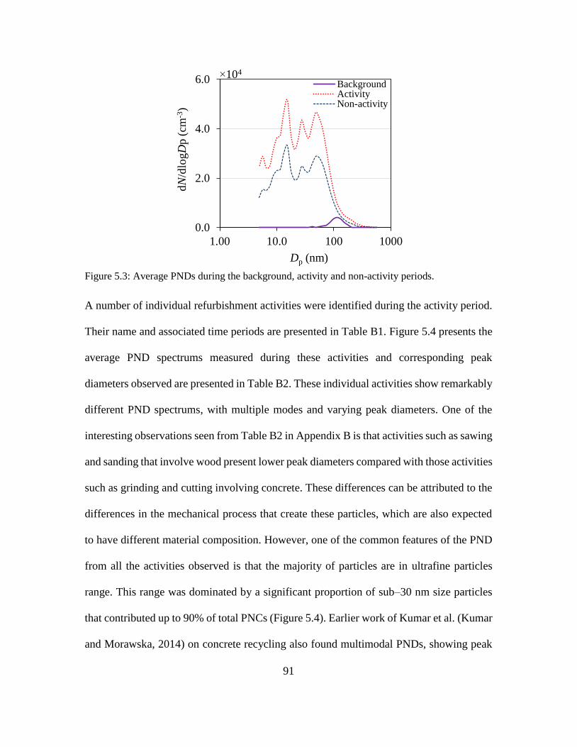
91
Figure 5.3: Average PNDs during the background, activity and non-activity periods.
A number of individual refurbishment activities were identified during the activity period.
Their name and associated time periods are presented in Table B1. Figure 5.4 presents the
average PND spectrums measured during these activities and corresponding peak
diameters observed are presented in Table B2. These individual activities show remarkably
different PND spectrums, with multiple modes and varying peak diameters. One of the
interesting observations seen from Table B2 in Appendix B is that activities such as sawing
and sanding that involve wood present lower peak diameters compared with those activities
such as grinding and cutting involving concrete. These differences can be attributed to the
differences in the mechanical process that create these particles, which are also expected
to have different material composition. However, one of the common features of the PND
from all the activities observed is that the majority of particles are in ultrafine particles
range. This range was dominated by a significant proportion of sub–30 nm size particles
that contributed up to 90% of total PNCs (Figure 5.4). Earlier work of Kumar et al. (Kumar
and Morawska, 2014) on concrete recycling also found multimodal PNDs, showing peak
Dp (nm)
dN
/dlo
gD
p(c
m-3
)
0.0
2.0
4.0
6.0
1.00 10.0 100 1000
BackgroundActivityNon-activity
104
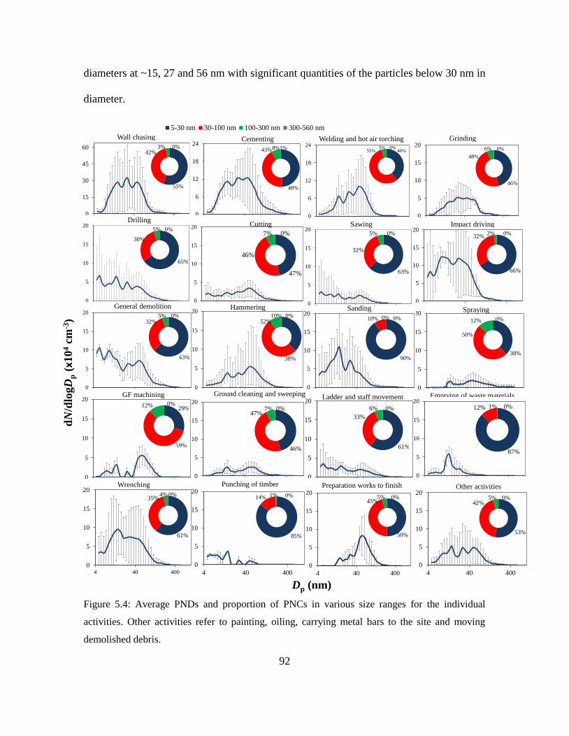
92
diameters at ~15, 27 and 56 nm with significant quantities of the particles below 30 nm in
diameter.
Figure 5.4: Average PNDs and proportion of PNCs in various size ranges for the individual
activities. Other activities refer to painting, oiling, carrying metal bars to the site and moving
demolished debris.
0
5
10
15
20
4 40 400
0
5
10
15
20
4.00 40.0 4000
5
10
15
20
4.00 40.0 400
Wall chasing
Ground cleaning and sweeping Emptying of waste materialsLadder and staff movement
0
5
10
15
20
4 40 400
x 1
00
00
65%
30%
5% 0%
0
5
10
15
20
4.00 40.0 400
Cutting
0
5
10
15
20
4.00 40.0 400
63%
32%
5% 0%
0
5
10
15
20
4.00 40.0 400
General demolition
63%
32%5% 0%
0
5
10
15
20
4.00 40.0 400
38%
52%10% 0%
0
6
12
18
24
4.00 40.0 400Sawing
GF machining
29%
59%
12% 0%
0
15
30
45
60
4.00 40.0 400Drilling
Welding and hot air torching
55%
42%3% 0%
0
5
10
15
20
4.00 40.0 400
38%
50%
12% 0%
0
5
10
15
20
4.00 40.0 400
87%
12% 1% 0%
0
6
12
18
24
4.00 40.0 400
Cementing
48%
43%8%1%
0
5
10
15
20
4.00 40.0 400
SandingHammering
90%
10% 0% 0%
47%
46%
7% 0%
Spraying
40%55%5% 0%
0
5
10
15
20
4.00 40.0 400
46%
47%7% 0%
Wrenching
48%43%
8%1%
5-30 nm 30-100 nm 100-300 nm 300-560 nm
Grinding
0
5
10
15
20
4.00 40.0 400
46%
48%
6% 0%
Impact driving
0
5
10
15
20
4.00 40.0 400
66%
32%2% 0%
61%
33%
6% 0%
0
5
10
15
20
4 40 400
53%
42%5% 0%
Other activities
0
5
10
15
20
4 40 400
Punching of timber
85%
14% 1% 0%
0
5
10
15
20
4 40 400
Preparation works to finish
50%
45%5% 0%
61%
35%4%0%
dN
/dlo
gD
p(x
10
4cm
-3)
Dp (nm)

93
Wall chasing activity was observed to produce a greatest concentration in terms of release
of new particles, reflecting the effect of abrasion between the wall surface and the chasing
drill material. An overall increase over the background levels (Figure 5.4) during these
activities clearly indicates the emissions of new particles. However, these results did not
allow us to draw conclusions on their formation pathways, i.e. whether these emissions are
arising from electric motors of different tools used such as those analysed by He et al.
(2004) or through other novel mechanism, suggesting a need of dedicated studies in future.
In addition, transformation processes such as coagulation, condensation, nucleation and
deposition act simultaneously on the number and size distributions of particles. These
processes lead to both increase (e.g. nucleation) and decrease (e.g. coagulation and
deposition) in PNCs (Kumar et al., 2011a). Coagulation is an aggregation of particles and
this aggregation is a function of both the residence time of particles in an experimental
setting and their ambient number concentrations (Hinds, 1999). A typical average
concentration was measured in the range of ~104 cm–3 (Section 5.3.2) with the highest
PNCs being of the order of ~106 cm–3 during wall chasing (see Table B3 in Appendix B).
The time taken for the 104 and 106 cm–3 in doubling the size of particles through
monodisperse coagulation is about 16 days and 4h, respectively (Hinds, 1999). This time
is much greater than both the sampling rate (10 Hz) and the air exchange rates at the site (a
few 10’s of minutes), meaning that the effect of aggregation on measured PNCs can be
overlooked.

94
5.3.2 Particle number concentrations
Average PNCs on a daily basis including background, activity and non-activity
periods are summarised in Table 5.2 and their proportions in various size ranges are shown
in Figure 5.5. The overall average PNCs (49.14±32.80 ×10³) during the activity periods
were significantly above the background level (1.17±0.80 ×10³) and showed noteworthy
variation from day to day with maximum values being about twice the average. However,
the fraction of average PNCs in the 5–30 nm, 30–100 nm and 100–300 nm ranges during
the activity and non-activity periods remained nearly unchanged Figure 5.5. There was a
much larger change to PNCs in the 5–30 nm size range that, for example, increased from
~0.2% during background to 56 and 55% during activity and non–activity periods,
respectively. Such a change was modest (within 6%) between background and activity/non-
activity periods for the particles in the 30–100 nm range.
Figure 5.5: Average PNCs during the background, activity and non-activity periods.
0
3
6
9
12
15
18
Background Activity Non-activity
PN
C (
# c
m-3
)
104
56%
39%
5%
55%40%
5%
5- 30 nm 30- 100 nm 100- 300 nm 300-560 nm
34%
66%
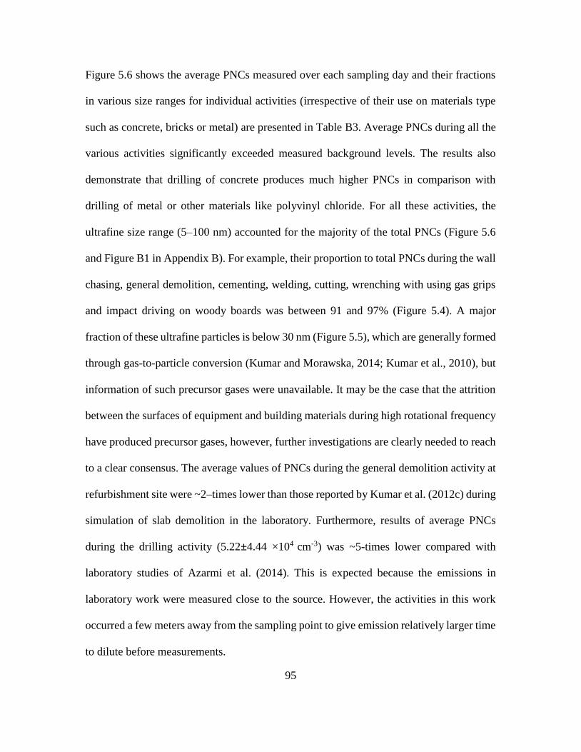
95
Figure 5.6 shows the average PNCs measured over each sampling day and their fractions
in various size ranges for individual activities (irrespective of their use on materials type
such as concrete, bricks or metal) are presented in Table B3. Average PNCs during all the
various activities significantly exceeded measured background levels. The results also
demonstrate that drilling of concrete produces much higher PNCs in comparison with
drilling of metal or other materials like polyvinyl chloride. For all these activities, the
ultrafine size range (5–100 nm) accounted for the majority of the total PNCs (Figure 5.6
and Figure B1 in Appendix B). For example, their proportion to total PNCs during the wall
chasing, general demolition, cementing, welding, cutting, wrenching with using gas grips
and impact driving on woody boards was between 91 and 97% (Figure 5.4). A major
fraction of these ultrafine particles is below 30 nm (Figure 5.5), which are generally formed
through gas-to-particle conversion (Kumar and Morawska, 2014; Kumar et al., 2010), but
information of such precursor gases were unavailable. It may be the case that the attrition
between the surfaces of equipment and building materials during high rotational frequency
have produced precursor gases, however, further investigations are clearly needed to reach
to a clear consensus. The average values of PNCs during the general demolition activity at
refurbishment site were ~2–times lower than those reported by Kumar et al. (2012c) during
simulation of slab demolition in the laboratory. Furthermore, results of average PNCs
during the drilling activity (5.22±4.44 ×104 cm-3) was ~5-times lower compared with
laboratory studies of Azarmi et al. (2014). This is expected because the emissions in
laboratory work were measured close to the source. However, the activities in this work
occurred a few meters away from the sampling point to give emission relatively larger time
to dilute before measurements.

96
Figure 5.6: The Average PNCs on a daily basis during the background, activity and non-activity
periods. The inner and outer circles represent fractions of PNCs in various size ranges during the
activity and non-activity periods, respectively.
Table 5.2: Average values of PNCs during the background, activity and non-activity periods on
different days.
Activity days Background PNC during activity periods
± Standard deviation (# cm-3 )
PNC during non-activity periods
± Standard deviation (# cm-3 )
1.17±0.80 ×10³ --- ---
1
--- 21.37±9.34 ×10³
11.33±9.63 ×10³
2
--- 26.99±27.18 ×10³
5.60±3.70 ×10³
3
--- 34.09±22.07 ×10³
27.90±20.06 ×10³
4
--- 20.357±15.11 ×10³
10.89±6.66 ×10³
5
---
97.84±129.50 ×10³
48.76±42.31 ×10³
6
--- 91.04±51.07 ×10³
68.24±42.74 ×10³
7 --- 52.31±39.68 ×10³ 41.27±33.65 ×10³
Overall average
1.17±0.80 ×10³ 49.14±32.80 ×10³ 30.57±23.28 ×10³
0.0
0.4
0.8
1.2
1.6
2.0
2.4
Background Day 1 Day 2 Day 3 Day 4 Day 5 Day 6 Day 7
Activity
Non-activity
PN
C (
# c
m-3
)
34%66% 66 %
32 % 2% 6
0 %
37
%
3%
54 %
40 %
6% 87
%
12%1%
68 %2
7 % 5%
57
%
37
%
6%
33 %
54
%
12%
1% 37 %
52
%
11%
57
%40
%
3%
54 %
42 %
4%4
3 %
50
%
7%
33 %
59
%
8%
62
%33
% 5% 6
7 %2
9
%
4%
66
%
32
%
2%0%
60 %
37 %
3%0%
5-30 nm 30-100 nm 100-300 nm 300-560 nm
105

97
5.3.3 Particle mass concentrations
Figure 5.7 shows the overall average of PM10, PM2.5 and PM1 during the
background, activity and non-activity periods. These PM fractions were found to be
significantly above the background levels (Table 5.3). For instance, PM10, PM2.5 and PM1
were up to 2- and 43-times larger during the activity periods than those during subsequent
periods of non-activity and background, respectively (Figure 5.8). Results of this study are
not directly comparable to other studies, but similar trend in increased concentrations were
observed by the other field studies. For example, Hansen et al. (2008) found a 2.9- and 3.3-
times increase in concentration for particles larger than 0.5 and 0.1 μm in size, respectively,
during the demolition of a hospital building. The average PM10 concentrations measured
during refurbishment activities found to exceed by about 20-times the 24-h mean European
limit values of 50 μg m−3 (Directive, 1999).
Figure 5.7: The concentrations of PM10, PM2.5 and PM1 during the background, activity and non-
activity periods.
PM
10;
PM
2.5
; P
M 1
(µg m
-3)
0
0.3
0.6
0.9
1.2
1.5
PM10 PM2.5 PM1
Background Activity Non-activity
103
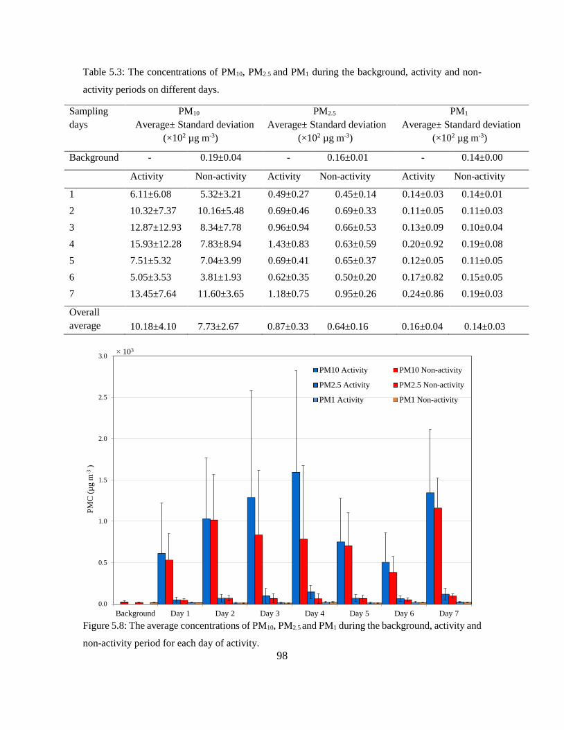
98
Table 5.3: The concentrations of PM10, PM2.5 and PM1 during the background, activity and non-
activity periods on different days.
Sampling
days
PM10
Average± Standard deviation
(×102 µg m-3)
PM2.5
Average± Standard deviation
(×102 µg m-3)
PM1
Average± Standard deviation
(×102 µg m-3)
Background - 0.19±0.04 - 0.16±0.01 - 0.14±0.00
Activity Non-activity Activity Non-activity Activity Non-activity
1 6.11±6.08 5.32±3.21 0.49±0.27 0.45±0.14 0.14±0.03 0.14±0.01
2 10.32±7.37 10.16±5.48 0.69±0.46 0.69±0.33 0.11±0.05 0.11±0.03
3 12.87±12.93 8.34±7.78 0.96±0.94 0.66±0.53 0.13±0.09 0.10±0.04
4 15.93±12.28 7.83±8.94 1.43±0.83 0.63±0.59 0.20±0.92 0.19±0.08
5 7.51±5.32 7.04±3.99 0.69±0.41 0.65±0.37 0.12±0.05 0.11±0.05
6 5.05±3.53 3.81±1.93 0.62±0.35 0.50±0.20 0.17±0.82 0.15±0.05
7 13.45±7.64 11.60±3.65 1.18±0.75 0.95±0.26 0.24±0.86 0.19±0.03
Overall
average 10.18±4.10 7.73±2.67
0.87±0.33 0.64±0.16 0.16±0.04 0.14±0.03
Figure 5.8: The average concentrations of PM10, PM2.5 and PM1 during the background, activity and
non-activity period for each day of activity.
0.0
0.5
1.0
1.5
2.0
2.5
3.0
Background Day 1 Day 2 Day 3 Day 4 Day 5 Day 6 Day 7
PM10 Activity PM10 Non-activity
PM2.5 Activity PM2.5 Non-activity
PM1 Activity PM1 Non-activity
103
PM
C (
µg
m-3
)

99
0.0
0.1
0.1
0.2
0.3
0.4
0.4
0.0
1.0
2.0
3.0
4.0
5.0
6.0
14:00:00 14:24:29 14:48:58 15:13:27 15:37:56 16:02:24
PM10
PM2.5
PM1
102 102
PM
10;
PM
2.5
(µg
m-3
)
PM
1(µ
g m
-3)
0.0
0.1
0.1
0.2
0.3
0.4
0.4
0.0
0.1
0.2
0.3
0.4
0.5
0.6
12:04:02 13:16:02 14:28:02 15:40:02 16:52:02 18:04:02
PM10
PM2.5
PM1
104 102
0.0
0.2
0.4
0.6
0.8
1.0
1.2
0.0
0.3
0.6
0.9
1.2
1.5
1.8
09:07:12 10:04:48 11:02:24 12:00:00 12:57:36 13:55:12
PM10
PM2.5
PM1
0.0
0.5
1.0
1.5
2.0
2.5
3.0
0.0
0.4
0.8
1.2
1.6
2.0
2.4
08:57:50 10:38:38 12:19:26 14:00:14 15:41:02 17:21:50
PM10
PM2.5
PM1
102 104
104 102
Drilling of concrete beam
Concrete drilling
GF machining
Time (s)
figure continues on next page

100
Figure 5.9: The concentrations of PM10, PM2.5 and PM1 during the background and activity period
(details of each activity time period is listed in Table B1).
PM
10;
PM
2.5
(µg
m-3
)
PM
1(µ
g m
-3)
0.0
3.0
6.0
9.0
12.0
15.0
18.0
0.0
0.3
0.6
0.9
1.2
1.5
1.8
09:36:00 10:00:29 10:24:58 10:49:26 11:13:55 11:38:24
PM10
PM2.5
PM1
0.0
1.2
2.4
3.6
4.8
6.0
7.2
0.0
0.2
0.3
0.5
0.6
0.8
0.9
09:30:14 10:13:26 10:56:38 11:39:50 12:23:02 13:06:14
PM10
PM2.5
PM1
104 102
104 102
Oiling of instrument
Carrying metal bars to the site
Wall chasing
0.0
0.3
0.6
0.9
1.2
1.5
0.0
0.1
0.1
0.2
0.3
0.4
0.4
10:47:17 11:44:53 12:42:29 13:40:05 14:37:41 15:35:17
PM10
PM2.5
PM1
104 102
0.0
0.7
1.4
2.1
2.8
3.5
4.2
0.0
0.1
0.3
0.4
0.6
0.7
0.8
10:25:55 11:52:19 13:18:43 14:45:07 16:11:31 17:37:55
Hu
nd
red
s
PM10
PM2.5
PM1
104 102
Opening cement packages
Drilling of concrete beam with VEKA
Drilling of concrete
Ladder movement
Time (s)
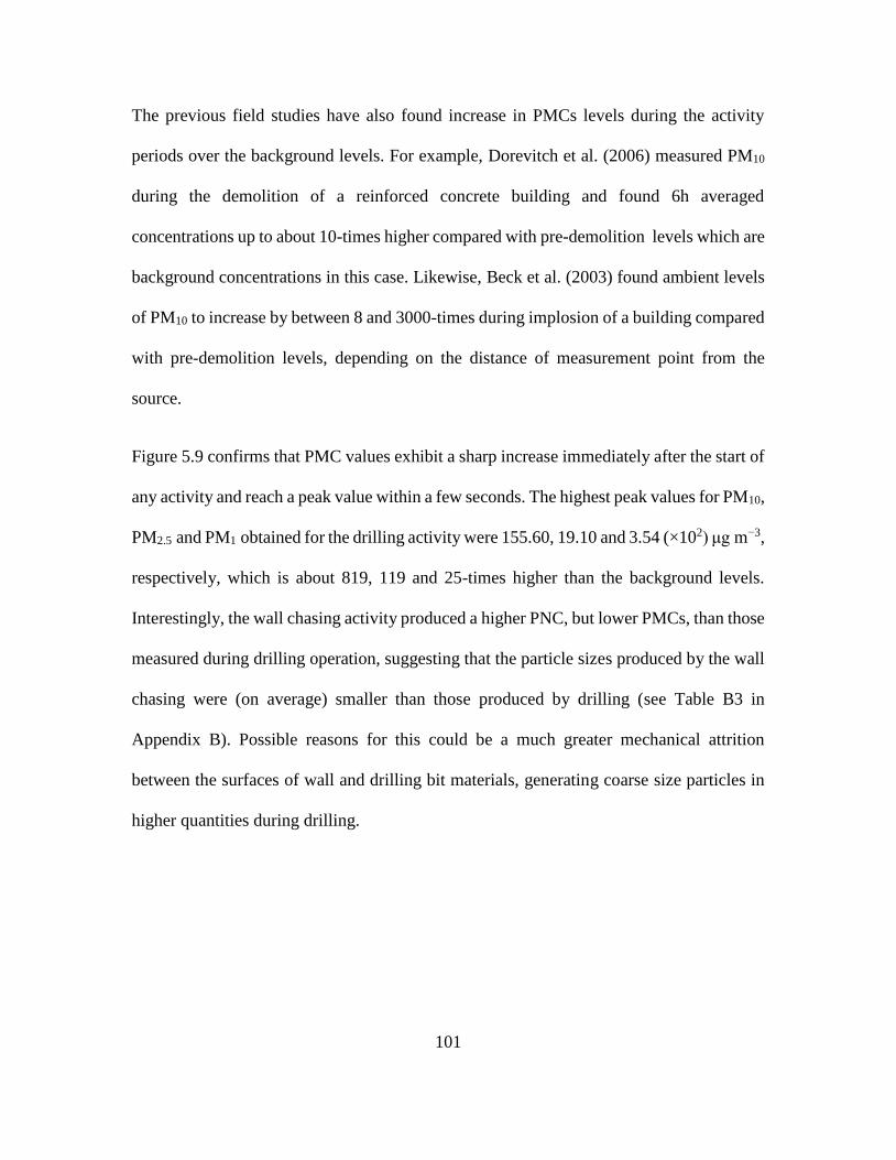
101
The previous field studies have also found increase in PMCs levels during the activity
periods over the background levels. For example, Dorevitch et al. (2006) measured PM10
during the demolition of a reinforced concrete building and found 6h averaged
concentrations up to about 10-times higher compared with pre-demolition levels which are
background concentrations in this case. Likewise, Beck et al. (2003) found ambient levels
of PM10 to increase by between 8 and 3000-times during implosion of a building compared
with pre-demolition levels, depending on the distance of measurement point from the
source.
Figure 5.9 confirms that PMC values exhibit a sharp increase immediately after the start of
any activity and reach a peak value within a few seconds. The highest peak values for PM10,
PM2.5 and PM1 obtained for the drilling activity were 155.60, 19.10 and 3.54 (×102) μg m−3,
respectively, which is about 819, 119 and 25-times higher than the background levels.
Interestingly, the wall chasing activity produced a higher PNC, but lower PMCs, than those
measured during drilling operation, suggesting that the particle sizes produced by the wall
chasing were (on average) smaller than those produced by drilling (see Table B3 in
Appendix B). Possible reasons for this could be a much greater mechanical attrition
between the surfaces of wall and drilling bit materials, generating coarse size particles in
higher quantities during drilling.
102
5.4 Morphology assessment and chemical characterization
SEM, IBA and XPS experiments were conducted on the samples collected on the
filters for understanding the morphology and chemical composition of particles such as
their shape, structure and chemical composition.
5.4.1 XPS and SEM analysis
Table 5.4 shows the elemental composition of all the five samples described in
Table 5.1. The blank filter sample and background contained the main characteristics of
Teflon type materials. The shape of the spectrum (see Figure B2 in Appendix B) indicated
a thin layer of about 5 mm on the background and blank filters. A very strong peak for
fluorine (F) was observed, followed by carbon (C) and oxygen (O) in the background
(sample 3) and blank (sample 4) filters. The samples 1, 2 and 5, which were taken during
activity periods, also contained calcium (Ca), silicon (Si), copper (Cu), aluminium (Al) and
sulphur (S).
The chemical state of Si can be associated to either organosilane or silicon dioxide (SiO2),
depending on the binding energy of the peak (see Figure B2). This is because Si is capable
of reacting with an organic compound and it is found to be present in an oxide form. Some
of the Al and S compounds and organic hydrocarbons were also found on the surfaces of
the filters collected during activity periods (i.e. samples 1, 2 and 5), which were thought of
arising from activities such as drilling of aluminium or steel stuff, spraying (galvanizing),
cementing and cutting of concrete.

103
Table 5.4: The elemental composition of the all the filters (quantitative XPS analyses).
Sample 1 Sample 2 Sample 3
(background)
Sample 4
(blank)
Sample 5
Name Fraction
(%)
Name Fraction
(%)
Name Fraction
(%)
Name Fraction
(%)
Name Fraction
(%)
C 37.4 C 34.9 C 31.2 C 30.3 C 34.3
O 11.1 O 8.2 O 1.2 O 1.0 O 21.5
F 50.5 F 55.3 F 67.6 F 68.7 F 37.5
Ca 0.9 Ca 0.6 Ca 1.5
Si 0.5 Si 2.2
Cu 0.2 Cu 0.3
S 0.4 S 1.2
Al 2.0
Further analysis showed that the sample 5 contained relatively heavier particles of elements
such as Cu. In addition, the intensity of the peaks of other elements such as C, Si and Al
was found to be increasing, mainly due to the longer exposure time and thereby leading to
larger amount of absorbed particles on the filter. Considering (i) the increment in the
intensity of O peak, (ii) its ratio with other peaks such as Si, Al and Ca, and (iii) comparison
of the shape of the C1s peak and all the fitted peaks contributing toward it, suggested that
these elements appear to be associated with grinding, drilling and welding activities where
aluminium oxide, calcium oxide, calcium carbonate, copper oxide compounds are expected
to be produced.

104
Figure 5.10: SEM images of (a) blank filter at ×500, (b) background measurements at ×8000, (c)
sample 1 at ×1000, (d) sample 1 at ×8000, (e) sample 2 at ×600, (f) sample 2 at ×8000, (g) sample
5 at ×8000, and (h) sample 5 at ×16000.
(a) (b)
(d)(c)
(e) (f)
(h)(g)
500 8000
1000 8000
600 8000
8000 16000
10 µm 1 µm
10 µm 1 µm
10 µm 1 µm
1 µm 1 µm

105
SEM images of the particles collected on filters were taken for understanding the
morphology of particles (Figure 5.10). A heterogeneous structure of the sampled particles
was found where the irregular shaped aggregated and spongy particles can be seen. A few
irregular shaped black holes can also be seen, which represent the porosity of the filters.
Differences between particles deposited on the background (sample 3) and blank (sample
4) filters and those collected during the activity periods (samples 1, 2 and 5) represents the
presence of new elements (Ca, Si, Cu, S and Al) arising from the refurbishment activities,
and some of these elements could be in oxide form as evident by the presence of O
(Table 5.4).
5.4.2 IBA analysis
Weight of elemental contents in parts per million (ppm) together with analysis
uncertainties and the minimum level of detection (MLD) are shown in Table B4. The filters
analysed in this work were much thicker (~3500 µg cm-2) than expected (~1000 µg cm-2)
leading to degradation of the accuracy generally achievable for this kind of analysis (Cohen
et al., 1996). The Fe-containing nanoparticles tend to form large aggregates of tens of
microns size. The possible reason for the high presence of Ca, Si and K is thought to be
due to activities related with concrete material (e.g. drilling, cutting and general
demolition), which is typically made of cement, water, admixtures and aggregates (Kumar
and Morawska, 2014). Furthermore, cement is made of constituents such as silicon oxide
(SiO2), calcium oxide (CaO), aluminium oxide (Al2O3), ferric oxide (Fe2O3) and sulphate
(S) that acts to bind the components of concrete together. This forms a nonporous, highly
cohesive, complex structure containing 10–50 nm diameter capillary pores in well hydrated
form (Raki et al., 2010). This suggests that the breaking of concrete containing small pores

106
may produce particles in various size ranges, as seen in Figure 5.4 (Kumar and Morawska,
2014). The comparison between the results of this section with those presented in Section
5.4.1 shows that Fe and Zn were detected by the IBA but not by the XPS analyses. This
difference is possibly due to the different detection levels of sample depth between the IBA
and XPS analyses.
5.5 Exposure assessment
The size range of the measured particles and their concentration are key factors for
the assessment of occupational exposure to ultrafine and PM. The average respiratory
disposition doses of PNCs were estimated using the approach described in Section 3.5.1
for both constant and size-dependant DFs (see Section B3).
The constant and size-dependent DFs provided the total deposited doses as 5.70±5.42
×108 min−1, 2.86±2.17 ×10⁸ min−1 as well as 7.03±6.65 ×10⁸ min−1 and 3.57±2.72
×108 min−1 for refurbishment activities during the activity and non-activity periods,
respectively (see Table B5). These figures show much higher doses for the size-dependent
DFs compared to those obtained using the constant DFs (Figure 5.11), mainly due to
dominance of particles below 100 nm which is a fraction that also have the largest
deposition (ICRP, 1995). This highlights the importance of the availability of size
distributions for an accurate exposure assessment.

107
Figure 5.11: Respiratory tract deposition dose rate (# min−1) calculated using (i) a constant DF and
the average PNC during each activity and (ii) size-dependent DFs and average size-resolved PNCs.
Lack of exposure assessment studies during refurbishment works make it challenging to
directly compare results of this study with published literature. It was tried to pick the
closest possible exposure studies for putting the results in a broad perspective. For instance,
Kumar et al. (2014) summarised results of 45 sampling locations in 30 different European
cities to estimate the respiratory deposition doses of PNCs in urban roadside environments.
The corresponding values of such doses were found to be 5.20±1.32 ×10⁸ min–1 in roadside
European environments. Likewise, Joodatnia et al. (2013a) estimated the average
0 10 20 30 40 50 60
Background
Non-activity
Impact driving
Prepration to finish
Punching of timber
Sanding
Grinding
Cementing
Ladder and staff movement
Wrenching
Emptying of waste materials
Spraying
Wall chasing
Ground cleaning and sweeping
GF machining
Welding and hot air torching
Drilling
Cutting
Sawing
Hammering
General Demolition
Other activities Dose with variable DF
Dose with constant DF
5.50±5.09 108 min–1 (typical car-cabin
environment; Joodatnia et al., 2013a)
6.56±6.53 108 min–1(our average for all
the activity periods in building
refurbishment environment)
5.20±1.32 108 min–1 (typical roadside
urban environment; Kumar et. al., 2014)
Respiratory deposition doses ( 108 min-1)

108
respiratory doses as 5.50±5.09 ×10⁸ min−1 over 30 car journeys in Guildford, UK.
Respiratory deposited doses for refurbishment activities are nearly one and a half times
higher than those shown by both studies. These observations clearly indicate that the
occupational exposure to workers on refurbishment site is much higher than those
experienced in roadside environments. Needless to mention that emission sources (e.g.
tailpipe of vehicles) are closest to the roadsides and therefore already high PNCs are
expected at such locations (Fujitani et al., 2012; Kumar et al., 2008). For the first time the
above findings clearly highlight that workers at the refurbishment sites spend long hours
and they are exposed to much higher PNCs than those experienced in outdoor ambient or
micro-transport environments, indicating a clear need for limiting occupational exposure
at such sites.
5.6 Chapter summary and conclusions
A DMS50 and GRIMM were used to measure number and size distributions of
particles in the 5–10,000 nm size range released by numerous activities. While the DMS50
data was used to analyse the PNCs, the data measured from the GRIMM allowed us to
assess PMCs in PM10, PM2.5 and PM1 fractions. Mass of bulk particles were also collected
on the PTFE filters during background as well as activity periods for understand their
physicochemical properties. The objectives were to understand the number and mass
emission characteristics of particles in various size ranges during these building activities
and assess their physical and chemical properties. The following conclusions are drawn:
The refurbishment activities were found to release ultrafine particles at levels well-
above the local background PNCs. The ultrafine particles were found to dominate (91-

109
97%) the total PNCs. Average PNCs during the periods of refurbishment activities were
found up to 84-times higher than the average PNCs during the background period. The
largest PNCs were observed during the wall chasing activity, followed by the drilling
and general demolition activities (Table B3).
Results showed that highest mass concentrations of PM10, PM2.5 and PM1 (i.e. 20.01,
1.52, 0.18 ×10² μg m−3) were obtained during general demolition. The peak value of
PMC was observed up to about 815-times higher over the background value during the
drilling in comparison with the other activities. The mechanical attrition between the
surfaces of instrument and materials during the activities and re-suspension of existing
particles appears to be a likely source to produce larger-sized particles.
Combining the results of XPS, SEM and IBA gives the capability of characterising both
the micro- and nano-sized particles. The increase of the surface composition of new
peaks and decrease of the F and C-F peaks shows higher level of deposition of the
particles on the filter and that the Fe-containing particles tend to form aggregates of
few 10 µm. These analyses showed the presence of the elements such Ca, Si, Cu, K, S,
Zn and Al on the collected samples. These elements were presumably released from
the building equipment and materials (e.g. concrete, bricks and metals) involved in the
refurbishment activities.
Occupations exposure to workers on the building refurbishment sites were found to
contribute much higher exposure compared with typical roadside urban environments.
Peak respiratory deposition doses during activity periods were over two orders of

110
magnitude higher than those during the background periods, showing a broad diversity
in the emission strengths of various refurbishment activities.
The study presented hitherto missing information that the refurbishment activities produce
ultrafine particles in dominant proportions. These high levels of ultrafine particle suggest
that there is a need to design appropriate risk mitigation strategies to limit exposures of on-
site workers. Further information about the particle emissions from an outdoor field site
(i.e. construction site) can be found in Chapter 6.

111
Chapter 6. Outdoor construction activities
This chapter presents the results of measurements of PM10 and PM2.5 concentrations
arising from outdoor construction activities along with meteorological data on the
surrounding environment in London. The chapter also provides information on analysis
using bivariate concentration polar plots, followed by k-mean analysis.
6.1 Introduction
Construction developments in both the developing and developed world are
common. However, the impact of PM emitted in coarse and fine particle size range from
such activities on the surrounding areas is yet poorly understood. Construction and
demolition of structures is known to result in higher local concentrations of PM10, which
contains a wide variety of toxic organic substances and may adversely affect the respiratory
health of nearby residents (Anderson, 2009; Brunekreef and Holgate, 2002; Davila et al.,
2006; Heal et al., 2012; Loomis, 2000). There is also an increasing interest in PM2.5 since
it penetrates deeper into the lungs and is of even greater concern for human health
(Chaloulakou et al., 2003; Pekkanen et al., 1997; Pope, 2000). For this reason, exposure to
PM2.5 is globally the 9th most powerful risk factor for diseases burden (Lim et al., 2013;
Oberdörster, 2000). Further information about the health and environmental impacts of the
particle emissions is presented in Section 2.7 (Chapter 2). Until recently, only limited
research has focused on exposure to the PM10 and even less research on exposure to the

112
PM2.5 fractions arising from outdoor construction activities and understanding their
potential impact on local air quality (Table 2.1). As described in Section 2.4 in Chapter 2,
besides the construction activities, PM10 concentrations are also affected by the emissions
arising from local fugitive sources such as road works (Amato et al., 2009; Fuller et al.,
2002; Fuller and Green, 2004; Ho et al., 2003; Tian et al., 2007), vehicle exhaust (Abu-
Allaban et al., 2007; Cadle et al., 1999; Kean et al., 2000; Kumar et al., 2010; Kumar et al.,
2011a) and non-vehicle exhaust sources (Chow et al., 2006; Dall'Osto et al., 2011; Hopke
et al., 1980; Kumar and Morawska, 2014; Kumar et al., 2013; Saliba et al., 2010). At the
same time, many activities associated with the air and sea transportation produce particles
across the range of PM10 and PM2.5 (Andrews et al., 2010; Bates et al., 2008; Corbett et al.,
2007). A few studies have investigated the PM10 emissions arising from industrial sources
such as waste transfer stations (Barratt and Fuller, 2014). There are also a few studies
concerned with PM10 emissions arising from the outdoor construction activities (Beck et
al., 2003; Dorevitch et al., 2006; Hansen et al., 2008; Joseph et al., 2009). However, there
is still very little work focusing on the PM2.5 fractions arising from construction activities
(Muleski et al., 2005).
The importance of particle exposure from construction sources is expected to increase with
the ever growing world population (Egbu, 1999; Kousa et al., 2002a). In addition to
concerns associated with the short-term exposure to airborne PM at the time of construction
activities, there is also a potential for long-term exposure to PM that settles across the

113
nearby community and then is available for inhalation or ingestion after resuspension (Abu-
Allaban et al., 2006; Beck et al., 2003; Lioy et al., 2002).
European Union Directive (1999) set the targets to limit daily and annual mean values of
PM10 at the EU level for year 2004 and 2010 (Fuller and Green, 2004). The legal limit by
2005 was to achieve daily mean PM10 concentration of 50 µg m-3, not exceeded on more
than 35 occasions per year and annual mean values of 40 µg m-3. Also the target by 2010
was to achieve daily mean PM10 concentration of 50 µg m-3, not exceeded on more than 7
occasions per year and annual mean concentrations of 20 µg m-3. These target values to be
met by 2010 were not carried forward in the Directive 2008/50/EC (Directive, 2008). For
example, Fuller and Green (2004) noted that the PM10 emissions generated by building and
road works in and around London breached EU limits of daily mean PM10 concentrations
(50 μg m−3) on several occasions. In this work, a series of PM10 and PM2.5 measurements
at 17 monitoring stations around construction sites were carried out during 2002–2013 to
assess their impact on the air quality in surrounding areas.
6.2 Materials and methods
6.2.1 Description of the sites and sampling set ups
Measurements were carried out around three outdoor construction sites, which are
referred hereafter as CS1, CS2 and CS3, respectively. CS1, CS2 and CS3 covered an area of
about 260×104, 54×104 and 3×10⁴ m2, respectively (Figure 6.1). There were 17 monitoring
stations (i.e. MS1–MS17) around these three outdoor construction sites (CS1, CS2 and CS3),
which represented a diverse range of construction activities. The locations of the
114
monitoring stations around these sites are shown in Figure 6.1, but the specific details about
the location have been kept anonymous for the protection of confidential information.
Continuous air quality monitoring was carried out at 17 different monitoring stations
around three construction sites to measure the concentration of PM10 and PM2.5. The
measurements of PM concentrations analysed in this paper were during the periods of
construction, and there were no similar measurements made before and/or after
construction works. Measurements were undertaken continuously and divided into
working hours (referred to as working period) in weekdays between 08:00 and 18:00 h
(local time) and non-working hours (referred to as non-working period), which covered the
weekdays between 18:00 and 08:00 h and the weekends.
Data were collected over a period of about 4000 days for about 12 years between 2002 and
2013 at these 17 different monitoring sites around CS1-CS3 (Table 6.1). A diverse range of
construction works during the different phases of the construction were anticipated at the
studied sites. However, I did not have access to information of the different phases of the
construction processes at each site, except the overall duration of the works.
Data were analysed with reference to the EU Limit Values for annual and daily PM10
concentrations. In addition, bivariate plots were drawn to qualitatively assess the effects of
wind speed and direction on the measured concentrations in upwind and downwind
directions from construction sites. The k-means clustering technique was then applied to
assess contribution of probable local construction sources, which were identified through
bivariate polar plots of paired monitoring stations (i.e. one in upwind and the other in

115
downwind). The k-means clustering technique helped to identify the range of increments
in particle mass concentrations due to the construction operations, including the
resuspension and emissions from any on-site vehicles (Carslaw and Ropkins, 2012). Also
frequency and variation in PM10 and PM2.5 concentration in prevailing wind direction were
evaluated with changes in distance from sources by pairing the sites in downwind of the
CS1-CS3 in order to assess the decay profile of the PM emissions, which is important to
understand the impact of the construction works on the air quality in surrounding areas.
PM concentrations at CS1 were collected using TEOM 1400 and those at CS2 and CS3 were
measured by Osiris instrument (model 2315) as described in Sections 3.2.3 and 3.2.4 in
Chapter 3. Practical constraints such as space and cost, were important factors in the
instrument selection.
The meteorological data were produced taking a mean from a number of different
monitoring locations across the monitoring stations and construction areas where the
meteorological equipment is considered to be working well and the data shows a good
correlation. The measurements were made using cup anemometers and wind vanes (as
opposed to sonic anemometers) mainly made by Campbell Scientific. This equipment was
located at a height of about 10 m.
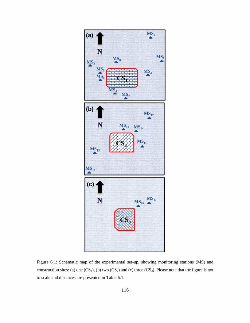
116
Figure 6.1: Schematic map of the experimental set-up, showing monitoring stations (MS) and
construction sites: (a) one (CS1), (b) two (CS2) and (c) three (CS3). Please note that the figure is not
to scale and distances are presented in Table 6.1.
MS1
MS2
MS3
MS4
MS5
MS6
MS7
MS8
MS10
MS11
MS12
MS13
MS14
MS15
MS17
CS1
CS3
CS2
MS9
MS16
(a)
(b)
(c)

117
Table 6.1: Description of monitoring stations around the construction sites. Monitoring stations S1-
S9, S10-S15, and S16-S17 below are around the CS1, CS2 and CS3, respectively.
Site
Code
Duration Species
Monitored
Instrument
used
Location
(distance of MS from
CS)
MS1 January 2002- January 2007 PM10 TEOM 1400 CS1 (3000 m)
MS2 January 2002- January 2007 PM10 TEOM 1400 CS1 (500 m)
MS3 January 2002- January 2007 PM10 TEOM 1400 CS1 (500 m)
MS4 January 2002- January 2007 PM10, PM2.5 TEOM 1400 CS1 (100 m)
MS5 January 2002- January 2007 PM10, PM2.5 TEOM 1400 CS1 (200 m)
MS6 January 2002- January 2007 PM10, PM2.5 TEOM 1400 CS1 (200 m)
MS7 January 2002- January 2007 PM10, PM2.5 TEOM 1400 CS1 (500 m)
MS8 January 2002- January 2007
PM10, PM2.5 TEOM 1400 CS1 (500 m)
MS9 January 2002- January 2007 PM10, PM2.5 TEOM 1400 CS1 (4000 m)
MS10 January 2009- December 2013 PM10 OSIRIS 2315 CS2 (100 m)
MS11 December 2009- May 2013 PM10 OSIRIS 2315 CS2 (200 m)
MS12 November 2008- December 2013 PM10 OSIRIS 2315 CS2 (1000 m)
MS13 January 2009- December 2013 PM10 OSIRIS 2315 CS2 (3000 m)
MS14 May 2013- December 2013 PM10 OSIRIS 2315 CS2 (100 m)
MS15 January 2009- October 2014 PM10 OSIRIS 2315 CS2 (400 m)
MS16 June 2011- August 2012
PM10 OSIRIS 2315 CS3 (100 m)
MS17 June 2011- August 2012 PM10 OSIRIS 2315 CS3 (50 m)

118
6.3 Results and discussion
6.3.1 Bivariate concentration polar plots
Bivariate polar plots were used to recognise different sources of PM and their
characteristics at the construction sites (Mouzourides et al., 2015; Westmoreland et al.,
2007). Figure 6.2 shows the polar plots that were constructed by partitioning wind speed
and direction data and their corresponding hourly mean PM concentration data into wind
speed and direction bins (Carslaw and Ropkins, 2012). These plots are presented as
smoothed surfaces showing variations in concentrations, depending on the local wind
direction and wind speed at a receptor (Carslaw and Beevers, 2013). The results presented
in Figure 6.2 show evidence of increased PM10 and PM2.5 concentrations levels when the
wind direction is from the construction sites to the monitoring stations.
Closer inspection of polar plots at all 17 monitoring stations around each of the three sites
indicates the following. Firstly, whenever there are monitoring stations in the downwind
side of the construction sites, high concentrations of PM10 (Figure 6.2) and PM2.5
(Figure 6.3) are seen, indicating a potential contribution from the construction activities
(Figure 6.2). Secondly, pockets of high PM concentrations can also be seen in some cases
(for example, see MS2 for PM10 and MS9 for PM2.5 in Figure 6.2a and Figure 6.3,
respectively) despite the monitoring stations being in the upwind of east and south-west
wind directions. This is expected due to long-range transport of PM10 during easterly winds
from European countries (Liu and Harrison, 2011; Smethurst et al., 2012) and the effect of
generated sea salt on PM2.5 from the south-westerly winds (Jones et al., 2010; Liu and
Harrison, 2011).

119
Figure 6.2: Polar plots for PM10 at the (a) CS1, (b) CS2 and (c) CS3; hourly average values during
24-h measurements were used for all pollutants. These plots present as smoothed surfaces how
concentrations vary depending on the local wind speed and wind direction.
MS1 MS2 MS3
MS4 MS5 MS6
MS7 MS8 MS9
(a)
(µg m – 3)

120
Figure 6.2: Polar plots for PM10 at the (a) CS1, (b) CS2 and (c) CS3; hourly average values during
24-h measurements were used for all pollutants. These plots present as smoothed surfaces how
concentrations vary depending on the local wind speed and wind direction.
MS10 MS11 MS12
MS13 MS14 MS15
(b)
MS17MS16
(c)
(µg m – 3)

121
This observation also suggest that the concentrations measured in downwind of
construction sites include some contribution of emissions from these sources and are not
solely the emissions from construction activities. However, this analysis is inadequate to
conclusively report that the measured downwind emissions are from construction.
Therefore, paired-site analysis (Section 6.3.2) and k-means cluster analysis (Section 6.3.3)
were performed to better understand the contributions of construction emissions during
varying wind directions.
Figure 6.3: Polar plots for PM2.5 (hourly average values during 24-h measurements were used for
all pollutants) at the CS1. These plots present as smoothed surfaces how concentrations vary
depending on the local wind speed and wind direction.
MS4 MS5 MS6
MS7 MS8 MS9
(µg m – 3)

122
6.3.2 Assessment of paired sites for examining differences in PM concentrations
The monitoring stations opposite to each other were paired in the upwind and
downwind of the construction sites to assess the relative change in the concentrations that
may have been contributed by the construction emissions (Figure 6.4). Two pairs of paired
monitoring stations were found each for PM10 and PM2.5 around CS1 (Figure 6.4a) and
another two pairs for PM10 around CS2 (Figure 6.4b), giving a total of 6 paired monitoring
stations. This pairing allowed us to measure changes in concentrations (i.e. ΔPM10 and
ΔPM2.5) as air mass crosses the construction sites and the results are presented in Figure 6.4.
For example, the hourly mean differences in PM10 and PM2.5 at CS1 measured in two pairs
of opposite monitoring stations (MS1, MS4 and MS7, MS8), which were estimated as MS4
minus MS1 and MS7 minus MS8. Likewise, hourly mean differences at CS2 were calculated
using MS14 and MS15 as opposite monitoring stations, which was MS15 minus MS14.
Subtraction of results in upwind polar plots from those in downwind polar plots clearly
shows increment in concentrations of PM10 and PM2.5 at all the sites, with all the values
being positive and high concentration zone reflecting emissions from construction sites.
Cross-comparison of results between different PM types suggest that the differences are
larger for coarse particles compared with fine particles, suggesting a relatively greater
extent of PM10 emissions than those of PM2.5 from construction works. Similar
observations were reported by previous studies (Font et al., 2014) where they found greater
increments in PM10 compared with PM2.5 from the road widening works in London.

123
Figure 6.4: The polar plots for the paired monitoring stations across each construction site, for
ΔPM10 and ΔPM2.5 (a) at the CS1 and (b) for ΔPM10 at the CS2, respectively.
MS1
MS7
MS8
CS1
MS4
(a)
(b)
MS15
CS2
MS14
ΔPM10 (MS15 – MS14)
ΔPM2.5 (MS7 – MS8)
MS11
ΔPM10 (MS11 – MS15)
MS2
ΔPM10 (MS4 – MS1)
ΔPM10 (MS6 – MS2)
6MS
MS5Δ
PM
2.5
(MS
5–
MS
7)
(µg m – 3)
(µg m – 3)
(µg m – 3)
(µg m – 3)
(µg m – 3)
(µg m – 3)

124
6.3.3 k-means clusters analysis
In order to identify and independently assess the contribution of local sources, k-
means cluster analysis was applied on the 6 paired monitoring stations that were identified
and discussed in Section 6.3.2. Eight different clusters were chosen that were found to be
optimal for separating the local source contribution from external sources, based on the
recommendations from previous studies (Carslaw and Beevers, 2013; Elangasinghe et al.,
2014; Everitt et al., 2011; Wood, 2006).
Figure 6.5 and Figure 6.6 show the contribution of each cluster in polar plots of ΔPM10 and
ΔPM2.5. Also are shown the temporal variation of ΔPM10 and ΔPM2.5 contributed by each
cluster on an hourly, weekly and monthly basis. Based on the ΔPM10 and ΔPM2.5
concentrations showing the high concentration peaks in polar plots (Figure 6.4), clusters
5–7 can be identified to represent the concentrations of ΔPM10 (Figure 6.5) and ΔPM2.5
(Figure 6.6) due to construction sources. If look at these clusters in the temporal variation
plots, peaks can be seen during the weekdays which are missing during the weekends. This
is also demonstrated by the increments in PM10 and PM2.5 concentrations during 08:00 and
18:00 h, which we referred to as “working hours”. While looking at the temporal plots on
a monthly basis, the identified clusters (i.e. 5-7) showed relatively lower concentrations
during the cold months (i.e. December, January and February) compared with the rest of
the months.

125
0
5
10 w ind spd.
15
20
25
W
S
N
E
cluster
12345678
0
5
10 w ind spd.
15
20
25
W
S
N
E
cluster
12345678
hour
NO
2
20406080
0 6 12 18 23
Monday
0 6 12 18 23
Tuesday
0 6 12 18 23
Wednesday
0 6 12 18 23
Thursday
0 6 12 18 23
Friday
0 6 12 18 23
Saturday
0 6 12 18 23
Sunday
1 2 3 4 5 6 7
hour
NO
2
20
30
40
50
60
0 6 12 18 23
month
NO
2
40
60
80
J F M A M J J A S O N D
weekday
NO
2
30
40
50
60
70
80
Mon TueWedThu Fri Sat Sun
mean and 95% confidence interval in mean
hour
PM
10
20
40
60
0 6 12 18 23
Monday
0 6 12 18 23
Tuesday
0 6 12 18 23
Wednesday
0 6 12 18 23
Thursday
0 6 12 18 23
Friday
0 6 12 18 23
Saturday
0 6 12 18 23
Sunday
1 2 3 4 5 6 7
hour
PM
10
20
30
40
50
0 6 12 18 23
month
PM
10
50
100
150
J F M A M J J A S O N D
weekday
PM
10
20
30
40
50
Mon Tue Wed Thu Fri Sat Sun
mean and 95% confidence interval in mean
hour
NO
2
20406080
0 6 12 18 23
Monday
0 6 12 18 23
Tuesday
0 6 12 18 23
Wednesday
0 6 12 18 23
Thursday
0 6 12 18 23
Friday
0 6 12 18 23
Saturday
0 6 12 18 23
Sunday
1 2 3 4 5 6 7
hour
NO
2
20
30
40
50
60
0 6 12 18 23
month
NO
2
40
60
80
J F M A M J J A S O N D
weekday
NO
2
30
40
50
60
70
80
Mon TueWedThu Fri Sat Sun
mean and 95% confidence interval in mean
hour
NO
2
20406080
0 6 12 18 23
Monday
0 6 12 18 23
Tuesday
0 6 12 18 23
Wednesday
0 6 12 18 23
Thursday
0 6 12 18 23
Friday
0 6 12 18 23
Saturday
0 6 12 18 23
Sunday
1 2 3 4 5 6 7
hour
NO
2
20
30
40
50
60
0 6 12 18 23
month
NO
2
40
60
80
J F M A M J J A S O N D
weekdayN
O2
30
40
50
60
70
80
Mon TueWedThu Fri Sat Sun
mean and 95% confidence interval in mean ΔPM10 (MS6 – MS2)
Hour
ΔP
M1
0 (µ
g m
-3)
ΔP
M1
0 (µ
g m
-3)
WeekdayMonth
MonthHour Weekday
0
5
10 w ind spd.
15
20
25
W
S
N
E
cluster
12345678
0
5
10 w ind spd.
15
20
25
W
S
N
E
cluster
12345678
(a) ΔPM10 (MS4 – MS1)
15
15
15
20
25
15
15
15
20
15
25
15
10
5
10
5

126
Figure 6.5: Clusters identified at CS1 and CS2 sites for PM10 concentrations for 8 clusters. The
shading shows the 95% confidence intervals in the mean. The data have been normalised in each
case by dividing by the mean.
hour
PM
2.5
0
50
100
150
0 6 12 18 23
Monday
0 6 12 18 23
Tuesday
0 6 12 18 23
Wednesday
0 6 12 18 23
Thursday
0 6 12 18 23
Friday
0 6 12 18 23
Saturday
0 6 12 18 23
Sunday
1 2 3 4 5 6 7 8
hour
PM
2.5
5
10
15
20
25
30
0 6 12 18 23
month
PM
2.5
15
20
25
30
35
J F M A M J J A S O N D
weekday
PM
2.5
15
20
25
30
35
40
Mon Tue Wed Thu Fri Sat Sun
mean and 95% confidence interval in mean
hour
PM
2.5
0
50
100
150
0 6 12 18 23
Monday
0 6 12 18 23
Tuesday
0 6 12 18 23
Wednesday
0 6 12 18 23
Thursday
0 6 12 18 23
Friday
0 6 12 18 23
Saturday
0 6 12 18 23
Sunday
1 2 3 4 5 6 7 8
hour
PM
2.5
5
10
15
20
25
30
0 6 12 18 23
month
PM
2.5
15
20
25
30
35
J F M A M J J A S O N D
weekday
PM
2.5
15
20
25
30
35
40
Mon Tue Wed Thu Fri Sat Sun
mean and 95% confidence interval in mean
0
5
10 w ind spd.
15
20
W
S
N
E
cluster
12345678
ΔP
M1
0 (µ
g m
-3)
ΔP
M1
0 (µ
g m
-3)
0
5
10 w ind spd.
15
20
25
W
S
N
E
cluster
12345678
0
5
10 w ind spd.
15
20
25
W
S
N
E
cluster
12345678
(b)
0
5
10 w ind spd.
15
20
25
W
S
N
E
cluster
12345678
Hour Month Weekday
hour
O3
5
15
25
0 6 12 18 23
Monday
0 6 12 18 23
Tuesday
0 6 12 18 23
Wednesday
0 6 12 18 23
Thursday
0 6 12 18 23
Friday
0 6 12 18 23
Saturday
0 6 12 18 23
Sunday
1 2 3 4 5 6 7
hour
O3
5
10
15
20
0 6 12 18 23
month
O3
5
10
15
20
25
J F M A M J J A S O N D
weekday
O3
5
10
15
20
MonTueWedThu Fri Sat Sun
mean and 95% confidence interval in mean
hour
O3
5
15
25
0 6 12 18 23
Monday
0 6 12 18 23
Tuesday
0 6 12 18 23
Wednesday
0 6 12 18 23
Thursday
0 6 12 18 23
Friday
0 6 12 18 23
Saturday
0 6 12 18 23
Sunday
1 2 3 4 5 6 7
hour
O3
5
10
15
20
0 6 12 18 23
month
O3
5
10
15
20
25
J F M A M J J A S O N D
weekday
O3
5
10
15
20
MonTueWedThu Fri Sat Sun
mean and 95% confidence interval in mean
Hour
hour
O3
5
15
25
0 6 12 18 23
Monday
0 6 12 18 23
Tuesday
0 6 12 18 23
Wednesday
0 6 12 18 23
Thursday
0 6 12 18 23
Friday
0 6 12 18 23
Saturday
0 6 12 18 23
Sunday
1 2 3 4 5 6 7
hour
O3
5
10
15
20
0 6 12 18 23
month
O3
5
10
15
20
25
J F M A M J J A S O N D
weekday
O3
5
10
15
20
MonTueWedThu Fri Sat Sun
mean and 95% confidence interval in mean
Month
hour
O3
5
15
25
0 6 12 18 23
Monday
0 6 12 18 23
Tuesday
0 6 12 18 23
Wednesday
0 6 12 18 23
Thursday
0 6 12 18 23
Friday
0 6 12 18 23
Saturday
0 6 12 18 23
Sunday
1 2 3 4 5 6 7
hour
O3
5
10
15
20
0 6 12 18 23
month
O3
5
10
15
20
25
J F M A M J J A S O N D
weekday
O3
5
10
15
20
MonTueWedThu Fri Sat Sun
mean and 95% confidence interval in mean
Weekday
ΔPM10 (MS11 – MS15)
ΔPM10 (MS15 – MS14)
15
15
15
15
15
20
15
25
20
15
25
10
5
10
5
hour
PM
2.5
0
50
100
150
0 6 12 18 23
Monday
0 6 12 18 23
Tuesday
0 6 12 18 23
Wednesday
0 6 12 18 23
Thursday
0 6 12 18 23
Friday
0 6 12 18 23
Saturday
0 6 12 18 23
Sunday
1 2 3 4 5 6 7 8
hour
PM
2.5
5
10
15
20
25
30
0 6 12 18 23
month
PM
2.5
15
20
25
30
35
J F M A M J J A S O N D
weekday
PM
2.5
15
20
25
30
35
40
Mon Tue Wed Thu Fri Sat Sun
mean and 95% confidence interval in mean
0 6 12 18 23 J F A J J S N DM M O MonTueWedThu Fri Sat SunA
5
10
15
20
25
30
15
20
25
30
35
15
20
25
30
35
40hour
PM
2.5
0
50
100
150
0 6 12 18 23
Monday
0 6 12 18 23
Tuesday
0 6 12 18 23
Wednesday
0 6 12 18 23
Thursday
0 6 12 18 23
Friday
0 6 12 18 23
Saturday
0 6 12 18 23
Sunday
1 2 3 4 5 6 7 8
hour
PM
2.5
5
10
15
20
25
30
0 6 12 18 23
month
PM
2.5
15
20
25
30
35
J F M A M J J A S O N D
weekday
PM
2.5
15
20
25
30
35
40
Mon Tue Wed Thu Fri Sat Sun
mean and 95% confidence interval in mean
20
40
60
0 6 12 18 23 0 6 12 18 23 0 6 12 18 23 0 6 12 18 23
Monday Tuesday Wednesday Thursday Friday Saturday Sunday

127
Figure 6.6: Clusters identified at CS1 for PM2.5 concentrations for 8 clusters. The shading shows the
95% confidence intervals in the mean. The data have been normalised in each case by dividing by
the mean.
hour
CO
0
1
2
3
0 6 12 18 23
Monday
0 6 12 18 23
Tuesday
0 6 12 18 23
Wednesday
0 6 12 18 23
Thursday
0 6 12 18 23
Friday
0 6 12 18 23
Saturday
0 6 12 18 23
Sunday
1 2 3 4 5 6 7
hour
CO
0.5
1.0
1.5
2.0
2.5
3.0
0 6 12 18 23
month
CO
0.5
1.0
1.5
2.0
2.5
J F M A M J J A S O N D
weekday
CO
1.0
1.5
2.0
2.5
MonTueWedThu Fri Sat Sun
mean and 95% confidence interval in mean
hour
CO
0
1
2
3
0 6 12 18 23
Monday
0 6 12 18 23
Tuesday
0 6 12 18 23
Wednesday
0 6 12 18 23
Thursday
0 6 12 18 23
Friday
0 6 12 18 23
Saturday
0 6 12 18 23
Sunday
1 2 3 4 5 6 7
hour
CO
0.5
1.0
1.5
2.0
2.5
3.0
0 6 12 18 23
month
CO
0.5
1.0
1.5
2.0
2.5
J F M A M J J A S O N D
weekday
CO
1.0
1.5
2.0
2.5
MonTueWedThu Fri Sat Sun
mean and 95% confidence interval in mean
hour
SO
2
5
10
15
0 6 12 18 23
Monday
0 6 12 18 23
Tuesday
0 6 12 18 23
Wednesday
0 6 12 18 23
Thursday
0 6 12 18 23
Friday
0 6 12 18 23
Saturday
0 6 12 18 23
Sunday
1 2 3 4 5 6 7
hour
SO
2
2
4
6
8
10
0 6 12 18 23
month
SO
2
2
4
6
8
J F M A M J J A S O N D
weekday
SO
2
2
4
6
8
MonTueWedThu Fri Sat Sun
mean and 95% confidence interval in mean
hour
SO
2
5
10
15
0 6 12 18 23
Monday
0 6 12 18 23
Tuesday
0 6 12 18 23
Wednesday
0 6 12 18 23
Thursday
0 6 12 18 23
Friday
0 6 12 18 23
Saturday
0 6 12 18 23
Sunday
1 2 3 4 5 6 7
hour
SO
2
2
4
6
8
10
0 6 12 18 23
month
SO
2
2
4
6
8
J F M A M J J A S O N D
weekday
SO
22
4
6
8
MonTueWedThu Fri Sat Sun
mean and 95% confidence interval in mean
ΔP
M2
.5 (µ
g m
-3)
ΔP
M2
.5 (µ
g m
-3)
0
5
10 w ind spd.
15
20
25
W
S
N
E
cluster
12345678
0
5
10 w ind spd.
15
20
25
W
S
N
E
cluster
12345678
Weekday
0
5
10 w ind spd.
15
20
25
W
S
N
E
cluster
12345678
ΔPM2.5 (MS7 – MS8)
0
5
10 w ind spd.
15
20
25
W
S
N
E
cluster
12345678
Hour Month
Hour
hour
CO
0
1
2
3
0 6 12 18 23
Monday
0 6 12 18 23
Tuesday
0 6 12 18 23
Wednesday
0 6 12 18 23
Thursday
0 6 12 18 23
Friday
0 6 12 18 23
Saturday
0 6 12 18 23
Sunday
1 2 3 4 5 6 7
hour
CO
0.5
1.0
1.5
2.0
2.5
3.0
0 6 12 18 23
month
CO
0.5
1.0
1.5
2.0
2.5
J F M A M J J A S O N D
weekday
CO
1.0
1.5
2.0
2.5
MonTueWedThu Fri Sat Sun
mean and 95% confidence interval in mean
Month Weekday
ΔPM2.5 (MS5 – MS7)
15
15
15
15
15
15
20
15
25
20
15
25
10
5
10
5

128
There could be two possible reasons for these lower concentrations: (i) lesser construction
activity compared to normal, and (ii) weather conditions suppressing the emissions and
transport of particles due to relatively wetter conditions than the other months, and also
affecting the normal construction due to adverse weather conditions. For example, mean
precipitation and relative humidity is expected to be higher during winter months (e.g. 256
mm and 85% to 213 mm and 70% during summer, respectively) and low temperature (e.g.
mean ~40C to 150C during summers) (Jenkins et al., 2009). Past studies have found wet
conditions such as water spraying an effective method to supress coarse particle emissions
by up to 13-times during construction works (Kumar et al., 2012c). Detailed receptor
modelling studies could help further in drawing firm conclusions.
6.3.4 Particle mass concentrations during working and non-working hours
Figure 6.7 shows the annual mean PM10 and PM2.5 concentrations at all the three
construction sites.
Figure 6.7: The annual average concentrations of PM10 (17 monitoring stations) during 2002-2013
period at the (a) CS1, (b) CS2, and (c) CS3.
0
15
30
45
60
PM10 PM2.5 PM10 PM10
CS1 CS2 CS3
Annual
aver
age
of
PM
10
and P
M2
.5 (µ
g m
–3)

129
The annual average in PM10 concentrations were found to be 22.96±3.37 μg m−3,
18.77±2.24 μg m−3 and 34.98±2.85 μg m−3 at CS1 (Table 6.2), CS2 (Table 6.4) and CS3
(Table 6.5), respectively, while the annual average PM2.5 concentrations were 14.01±1.76
μg m−3 at CS1 (Table 6.3). These averages include both the working and non-working hours
and the averages for these separate durations are presented in Figures C1a and C2 and
described in Appendix C, Sections C1-C2. Depending on the source and distance from the
monitoring stations, the values of PM10 and PM2.5 varied and the concentrations in all cases
increased as the working period started (see Figures C1-C4).
In general, concentrations during the working hours were higher than those during the non-
working hours (see Tables C1-C4), presumably due to construction activities and the other
emission sources such as road vehicles in operation during working hours. Overall, PM10
values were about ~24, 18 and 120% larger during the working periods compared with
those during non-working periods at the CS1, CS2 and CS3, respectively. Also at the CS1,
there was an increase of about 11% in PM2.5 values during the working period compared
with non-working periods (see Figure C2).

130
Table 6.2: The annual average concentrations of PM10 including the working and non-working
periods at the CS1; ± refers to standard deviation and “–” to the unavailability of data.
Monitoring stations
Year MS1 MS2 MS3 MS4 MS5 MS6 M S7 MS8 MS9
2002 _ 21.94±12.28 19.14±11.20 29.59±22.38 27.56±20.95 23.61±15.62 19.37±10.58 19.42±10.21 24.36±14.42
2003 _ 24.57±15.75 21.25±12.98 36.73±32.14 26.80±18.65 31.31±27.93 22.16±14.03 23.87±15.54 22.15±13.71
2004 19.18±11.59 21.25±11.99 17.32±9.52 28.94±23.59 21.81±13.14 25.15±25.55 18.72±11.33 20.56±11.83 25.91±17.08
2005 19.60±10.66 23.93±12.13 17.41±10.95 26.71±21.57 23.23±14.18 23.95±19.40 19.15±10.44 19.66±10.23 _
2006 20.45±11.21 24.51±23.57 18.82±9.86 24.88±18.03 24.51±20.86 22.96±15.56 20.67±10.83 21.22±11.77 _
Overall
average 19.96±11.15
23.24±15.14
18.79±10.90 29.37±23.54
24.78±17.56
25.39±20.81
20.02±11.44
20.95±11.92
24.14±9.04
Table 6.3: The annual average concentrations of PM2.5 including the working and non-working periods at
the CS1; ± refers to standard deviation and “–” to the unavailability of data.
Monitoring stations
Year MS1 MS2 MS3 MS4 MS5 MS6 MS7 MS8 MS9
2002 _ _ _ 17.3±17.9 13.0±8.0 12.5±8.0 12.0±8.1 11.8±7.2 12.6±7.9
2003 _ _ _ 15.5±13.6 14.5±10.3 14.0±9.9 14.2±10.4 15.5±10.7 17.4±10.1
2004 _ _ _ 17.0±18.4 12.6±7.4 11.5±7.9 11.5±7.4 12.1±7.5 19.4±13.3
2005 _ _ _ 15.4±16.3 12.9±8.2 11.9±8.2 11.9±7.5 12.0±7.4 _
2006 _ _ _ 14.6±12.9 13.0±8.0 12.1±8.0 12.1±7.8 12.9±7.4 _
Overall
average
_
_
_ 16.0±15.8 13.2±8.4
12.9±8.4
12.4±8.2 12.9±8.0 16.5±6.2

131
Table 6.4: The annual average concentrations of PM10 including the working and non-working
periods; ± refers to standard deviation and “–” to the unavailability of data.
Monitoring stations
Year MS10 MS11 MS12 MS13 MS14 MS15
2009 24.86±15.54 18.28±11.09 19.34±11.60 14.75±7.90 _ 15.55±9.22
2010 23.68±16.89 17.27±11.23 _ 15.74±13.93 _ 14.81±10.31
2011 25.10±18.34 18.78±12.69 _ 20.40±11.88 _ 20.05±13.24
2012 22.20±16.17 18.68±13.71 _ 16.42±9.77 _ 18.07±15.49
2013 19.71±12.86 15.64±9.40 _ 20.03±11.20 17.43±12.76 19.16±13.60
Overall
average 23.11±16.17 17.73±12.35 19.34±11.60
17.47±11.28 17.43±12.79
17.53±13.11
Table 6.5: The average concentrations of PM10 including the working and non-working periods at
the CS3; ± refers to standard deviation.
Monitoring stations
Year MS16 MS17
2011 37.36±33.08 35.39±31.24
2012 28.56±24.36 38.61±24.66
Overall average 32.96±19.31 34.98±18.16
Comparison of 24 hour average concentrations of PM10 with the EU Directive 2008/50/EC
(Directive, 2008), as described in Table 6.6, suggests a number of exceedences each year
(Table 6.7 and Figure C5). However, these exceedences are not expected to be due to
construction works alone, given that the winds were blowing from various directions
(Figure 6.1 and Figure 6.2) and the nearby sources could have also made contribution to
these exceedences. Therefore, the data was filtered based on the wind directions at each
monitoring station (Figure 6.8). The monitoring stations downwind of construction sites
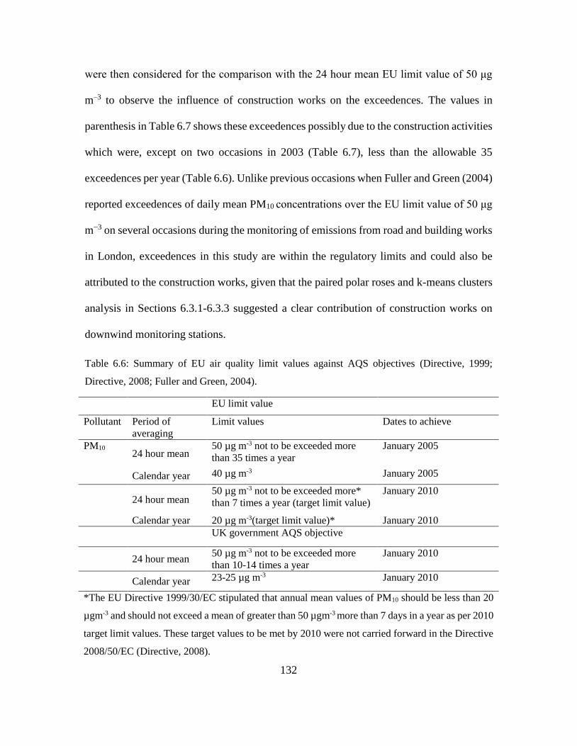
132
were then considered for the comparison with the 24 hour mean EU limit value of 50 μg
m–3 to observe the influence of construction works on the exceedences. The values in
parenthesis in Table 6.7 shows these exceedences possibly due to the construction activities
which were, except on two occasions in 2003 (Table 6.7), less than the allowable 35
exceedences per year (Table 6.6). Unlike previous occasions when Fuller and Green (2004)
reported exceedences of daily mean PM10 concentrations over the EU limit value of 50 μg
m−3 on several occasions during the monitoring of emissions from road and building works
in London, exceedences in this study are within the regulatory limits and could also be
attributed to the construction works, given that the paired polar roses and k-means clusters
analysis in Sections 6.3.1-6.3.3 suggested a clear contribution of construction works on
downwind monitoring stations.
Table 6.6: Summary of EU air quality limit values against AQS objectives (Directive, 1999;
Directive, 2008; Fuller and Green, 2004).
EU limit value
Pollutant Period of
averaging
Limit values Dates to achieve
PM10 24 hour mean
50 µg m-3 not to be exceeded more
than 35 times a year
January 2005
Calendar year 40 µg m-3 January 2005
24 hour mean
50 µg m-3 not to be exceeded more*
than 7 times a year (target limit value)
January 2010
Calendar year 20 µg m-3(target limit value)* January 2010
UK government AQS objective
24 hour mean
50 µg m-3 not to be exceeded more
than 10-14 times a year
January 2010
Calendar year 23-25 µg m-3 January 2010
*The EU Directive 1999/30/EC stipulated that annual mean values of PM10 should be less than 20
µgm-3 and should not exceed a mean of greater than 50 µgm-3 more than 7 days in a year as per 2010
target limit values. These target values to be met by 2010 were not carried forward in the Directive
2008/50/EC (Directive, 2008).

133
Figure 6.8: Numbers of exceedences over the EU limit value at the individual monitoring stations.
0 10 20 30 40 50 60
S10
S11
S12
S13
S14
S152013
2012
2011
2010
2009
Number of exceedences (days)
Mo
nit
ori
ng s
tati
on
s
MS1
MS1
MS1
MS1
MS1
MS1
MS1
MS1
MS1
MS1
MS10
MS11
MS12
MS13
MS14
MS15
MS16
MS17
0 10 20 30 40 50 60
S1
S2
S3
S4
S5
S6
S7
S8
S9 2006
2005
2004
2003
2002
MS1
MS2
MS3
MS4
MS5
MS6
MS7
MS8
MS9
EU limit value (not to be
exceeded 50 µg m-3 more
than 35 times a year)
0 10 20 30 40 50 60
S16
S17 20112010

134
Table 6.7: Number of exceeded days from the EU standard limit and UK government objective
(AQS). Please note that the excedances presented in the parenthesis against each exceedance
number represent the exceedances belonging to the 24 hours.
Monitoring Years
Monitoring
stations
2002 2003 2004 2005 2006 2007 2008 2009 2010 2011 2012 2013
MS1 0(0) 0(0) 2(2) 1(1) 0(0) _ _ _ _ _ _ _
MS2 3(2) 17(14) 3(1) 2(2) 5(3) _ _ _ _ _ _ _
MS3 1(0) 9 (7) 0(0) 1(1) 0(0) _ _ _ _ _ _ _
MS4 9(6) 60(48) 19(12) 11(7) 5(4) _ _ _ _ _ _ _
MS5 18(16) 22(16) 1(0) 6(6) 15(14) _ _ _ _ _ _ _
MS6 7(4) 42(36) 16(15) 9(6) 6(6) _ _ _ _ _ _ _
MS7 1(0) 11(7) 1(1) 1(1) 1(0) _ _ _ _ _ _ _
MS8 0(0) 14(12) 2(0) 1(0) 1(1) _ _ _ _ _ _ _
MS9 4(4) 6(5) 3(0) 0(0) 0(0)
MS10 _ _ _ _ _ _ _ 3(1) 17(3) 28(10) 12(12) 6(5)
MS11 _ _ _ _ _ _ _ 0(0) 11(7) 31(10) 16(14) 13(13)
MS12 _ _ _ _ _ _ _ 0(0) 0(0) 3(3) 5(4) 0(0)
MS13 _ _ _ _ _ _ _ 0(0) 0(0) 3(2) 1(1) 0(0)
MS14 _ _ _ _ _ _ _ 0(0) 0(0) 0(0) 0(0) 0(0)
MS15 _ _ _ _ _ _ _ 0(0) 0(0) 7(5) 6(5) 2(2)
MS16 _ _ _ _ _ _ _ _ _ 20(17) 4(4) _
MS17 _ _ _ _ _ _ _ _ _ 25(22) 33(22) _

135
6.3.5 Decay profiles of PM10 and PM2.5
The purpose of this section is to evaluate the variation in concentrations of PM10
and PM2.5 at different distances from the construction sites. This analysis assisted in
understanding how far the PM concentrations can go to affect the surrounding areas as well
as help in planning for emission mitigation measures, particularly for construction sites
close to sensitive areas such as hospitals or schools.
Figure 6.9 shows the decay profiles of PM10 and PM2.5 concentrations with the changing
distance from the CS1 and CS2. Both the logarithmic (Figure 6.9a) and exponential
(Figure 6.9b) best fit functions were applied to ΔPM10 and ΔPM2.5. The logarithmic decay
function (Figure 6.9a) was chosen as a best fit to the data based on better R2 values than
those given by an exponential decay profile as 0.79, 0.90 and 0.89 for PM10 (CS1), PM10
(CS2) and PM2.5 (CS1), respectively (Figure 6.9b). The differences between hourly averages
of PM10 and PM2.5 concentrations (ΔPM10 and ΔPM2.5) during the working and non-
working time periods provided the net concentrations from the construction activities,
which were then used to draw decay profiles (Figure 6.9). Further, the calculated
concentrations for PM10 and PM2.5 were filtered on the basis of prevailing wind direction.
The decay profile of PM10 concentrations at CS1 was drawn using the data measured at
MS4, MS5, MS7 and MS3 which were 100, 200, 500 and 1000 m away from the CS1,
respectively. Also the data measured at MS4, MS6 and MS7 were used to draw the decay
profile of PM2.5 at CS1 which were 100, 200 and 500 m away from the CS1. Furthermore
the decay profiles of PM10 concentrations were measured at 100, 200 and 400 m away from
the CS2 at MS10, MS11 and MS15, respectively.
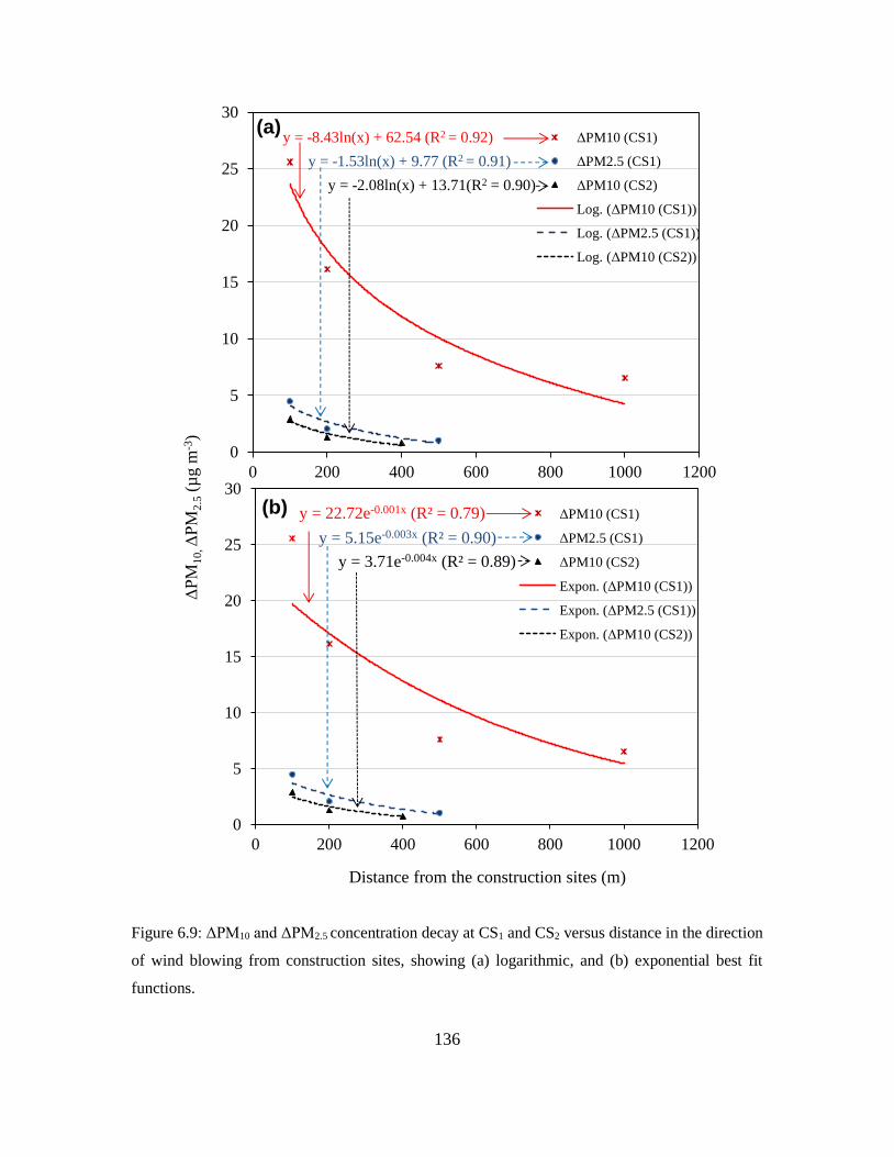
136
Figure 6.9: ΔPM10 and ΔPM2.5 concentration decay at CS1 and CS2 versus distance in the direction
of wind blowing from construction sites, showing (a) logarithmic, and (b) exponential best fit
functions.
y = -8.43ln(x) + 62.54 (R2 = 0.92)
y = -2.08ln(x) + 13.71(R2 = 0.90)
y = -1.53ln(x) + 9.77 (R2 = 0.91)
0
5
10
15
20
25
30
0 200 400 600 800 1000 1200
ΔPM10 (CS1)
ΔPM2.5 (CS1)
ΔPM10 (CS2)
Log. (ΔPM10 (CS1))
Log. (ΔPM2.5 (CS1))
Log. (ΔPM10 (CS2))
ΔPM
10
,ΔPM
2.5
(µg m
-3)
Distance from the construction sites (m)
(a)
y = 22.72e-0.001x (R² = 0.79)
y = 5.15e-0.003x (R² = 0.90)
y = 3.71e-0.004x (R² = 0.89)
0
5
10
15
20
25
30
0 200 400 600 800 1000 1200
ΔPM10 (CS1)
ΔPM2.5 (CS1)
ΔPM10 (CS2)
Expon. (ΔPM10 (CS1))
Expon. (ΔPM2.5 (CS1))
Expon. (ΔPM10 (CS2))
(b)

137
Because of atmospheric dilution, the mass concentration dramatically dropped with
increased distance from the construction site to approximately half of its value at a distance
between 100 and 200 m. The best fitting logarithmic decay equations for PM10 were drawn,
which gave R2 values as 0.92 and 0.91 for the CS1 and CS2, respectively (Figure 6.9a). A
much higher rate of change in PM concentrations can be seen close to the construction site
compared with those at farther distances. For instance, the rate of change in PM10 (CS1)
concentration with per meter distance is 0.06 μg m-3 in between 100 and 200 m, which
decreases to 0.030 and 0.013 μg m-3 per meter distance in the 200-400 m, and 400-1000 m
range, respectively (Figure 6.9a). These observations suggest to measure the PM within a
few 100 meter distance from the construction sites to capture the rapid decay in PMCs.
The total mean PM2.5 levels around the CS1 were also correlated well with the distances. A
logarithmic decay profile with R2 value of 0.90 represented the measured data very well.
Although studies measured decay of PM concentrations around the construction sites are
rare, it was tried to compare the data of this study with the most relevant studies. For
example, Hitchins et al. (2000) determined the PM10 concentration at increasing distances
from a road at two sites in Australia. They found that PM2.5 and ultrafine particles decayed
by up to half of their maximum initial concentrations within a distance of 100–150 m from
the road. Likewise, Buonanno et al. (2009) found PM10 concentration values to decrease
exponentially away from the freeway in Italy during weekly traffic conditions.
6.4 Chapter summary and conclusions
OSIRIS (model 2315) and TEOM 1400 were used to measure mass concentration
of particles in the 0.1–10 µm size range around the three construction sites at 17 monitoring

138
stations over a period of 12 years between January 2002 and December 2013. The
objectives were to understand the emission characteristics of coarse and fine particles from
the construction activities, identifying contribution to the ambient levels of PM
concentrations in the vicinity of these sites, and their spatial decay away from the
construction sites.
The following conclusions are drawn from this work:
The source characteristics of PM10 and PM2.5 were investigated using bivariate
concentration polar plots and k-means clustering techniques. The high concentrations
of PM10 and PM2.5 were observed at the paired monitoring stations during the
construction works when the winds were blowing from construction sites toward the
monitoring stations. K-means clustering technique provided a useful development to
the bivariate polar plots to assess the contribution of construction and other local
sources.
Three clusters (5, 6 and 7) from a total of selected 8 clusters showed strong evidences
of a downward increase in PM10 and PM2.5 levels during the weekdays. These clusters
were identified to represent construction activities.
PM10 were found about ~24, 18 and 120%, and PM2.5 about 11%, larger during the
working periods compared with those during non-working periods at the CS1, CS2 and
CS3, respectively. These increments were attributed to the construction works as
indicated by the bivariate concentration polar plots and k-means clustering analysis. In
addition, downwind concentrations of PM10 were found to be relatively more
influenced by construction works at the CS1 than PM2.5 concentrations.
139
The 24-hour mean EU limit of value of 50 µgm-3 set by EU Directives for PM10 not to
be exceeded more than 35 times a calendar year was breached on two occasions due to
construction operations on downwind monitoring stations during measurements
between 2002 and 2013.
Both the total PM10 and PM2.5 values during the working periods in downwind direction
found to be well correlated with the distances with R2 values over 0.90 in a logarithmic
form. These concentrations reduced to half of their initial concentrations within a few
100 meters. This indicates that placing a monitoring station around a site within this
peripheral distance could help capturing the rapid decay of particles escaping from the
construction sites.
The result presented in this study highlight the contributions of PM10 and PM2.5 from
construction works. The increase in concentrations of PM10 and PM2.5 at the downwind
monitoring stations suggest that there is a need to design more detailed and appropriate risk
mitigation strategies to limit exposures to onsite workers and people who live in the
surrounding environment. Further research is required to monitor and understand the
emission levels of particles arising from other filed building works within urban areas in
order to establish suitable exposure limits for both on-site workers and passer-by urban
people. For this purpose, the measurements of particles during outdoor field activities (i.e.
building demolition works) were carried to assess particles emissions and also
physicochemical features which allows to differentiate between the properties of particles
from indoor and outdoor sources. The results are presented in Chapter 7.

140
Chapter 7. Outdoor building demolition activities
This chapter presents the results of release of PM10, PM2.5 and PM1 from outdoor
building demolition activities. The chapter also provides assessments of physicochemical
properties of those particle and potential impact on workers and individuals in the
surrounding.
7.1 Introduction
Construction and demolition waste contribute up to about 33% of the total waste
from all the streams; about half of which is demolition waste (Balaras et al., 2007).
Construction and demolition of structures generate in excess of 450 million tonnes of waste
each year in Europe, with about 53 million tonnes per year in the UK alone (Lawson et al.,
2001; Rao et al., 2007). However, the number of buildings demolished each year is
expected to increase by 4-fold by 2016 in the UK from the levels of about 20,000 per year
in 2008 (ECI, 2005; Roberts, 2008). This increased rate of building demolition could be
linked to growing population of the urban areas and the need for improvements to meet
new urban design guidelines and adopt building technologies (Balaras et al., 2007; Kumar
et al., 2015). For example, the global urban population is expected to increase by about
60% in 2035 from the 2013 levels (GroBmann et al., 2013; Kumar et al., 2013a).
Building demolition can be accomplished through either implosion or mechanical means
141
(e.g. excavator and wrecking ball). Demolition by both mechanical disruption (Dorevitch
et al., 2006) and implosion (Beck et al., 2003) produce significant amount of PM, but the
impact of implosion demolition on surrounding areas air quality is generally short-lived
and severe (Beck et al., 2003). Recent studies have shown that workers in construction
industry dealing directly with concrete and cement products are exposed to notable PM
emissions (Azarmi et al., 2014; Croteau et al., 2002; Flanagan et al., 2006; Kumar et al.,
2012b) compared with those working in metal and wood industries (Fischer et al., 2005;
Lim et al., 2010). There are sufficient evidences that activities such as demolition,
earthmoving and building renovation are important sources of PM and degrade the
surrounding air quality (Azarmi et al., 2015a; Beck et al., 2003; Font et al., 2014; Hansen
et al., 2008; Joseph et al., 2009; Muleski et al., 2005). In addition, PM pollution from
demolition activity can adversely impact the health of people living close to demolition
sites, especially when the measures to restrict particles released from sites are inadequate
(Kumar et al., 2012a). Therefore, assessment of PM exposure becomes even more
important when such sites are situated within the densely built residential areas or sensitive
areas such as schools and hospitals.
Understanding the chemical constituents, morphology (i.e. size, shape) and surface
properties of particles released from building demolition are important for determining
their toxicity and health effects (Lo et al., 2000; Senlin et al., 2008). Currently, limited
studies have reported physicochemical properties of particles released from the building
demolition and therefore this is taken up for investigation in this study. However, further
details about the physicochemical analysis of the particles from demolition and

142
construction sources is presented in Section 2.6 in Chapter 2. Health concerns related to
dust inhalation have led to a number of dust control and reduction initiatives in demolition
industry. The US EPA have provided specific emission factors for different operations such
as demolition, construction and mineral operations to control PM emissions (EPA, 2011).
In addition, the UK Health and Safety Executive (HSE) developed a good practice
guideline to limit exposure to hazardous substances at the demolition sites (HSE, 2006,
2011). Furthermore, at local level, “Best Practice Guidance” is produced by London
Councils in partnership with the Greater London Authority in the UK, which contains a
number of practical methods to control dust and emissions from demolition activities
(Authority and Councils, 2006). However, demolition sites can be situated within
extremely busy places where meeting regulatory expectations, or strictly following
associated guidelines, are often challenging.
In order to fill the existing research gaps in the literature, this study investigates the release
of PM10, PM2.5 and PM1 and associated exposure around a real-world building demolition
site. The aims were to: (i) quantify the emission and exposure rates of particles and their
dispersion in the downwind of demolished building, (ii) assess the horizontal decay of the
PM emissions, (iii) understand the physical and chemical properties, (iv) computation of
particle mass emission factors (PMEFs), and (v) determining the occupational exposure to
on-site workers and people in the close vicinity of the demolition site.

143
7.2 Materials and methods
7.2.1 Sampling set up and site description
PMCs were measured at the fixed-sites in the downwind of demolition site, around
the demolished building through the mobile monitoring as well as at different distances
(10, 20, 40 and 80 m) from the demolition site through sequential measurements
(Figure 7.1). Monitoring was also carried out inside the cabin of an excavator vehicle and
in on-site canteen offices for engineers. Figure 7.2 shows the sampling locations around
the demolition site, which was situated ~10 m away from a busy road that was closed during
the demolition activity (i.e. sampling period). The demolished building was 30×15×8 m
(length × breadth × height) and was located in Haywards Heath in West Sussex, United
Kingdom (Figure 7.2). Construction material of building floors, stairs and supporting
columns was reinforced concrete while the walls were made of brick. The data were
collected for a total of 54 working hours between 08:00 and 18:00 h (local time) over a
period of 7 days; of which, one day was without any activity that enabled us to evaluate
the local background levels.
Table 7.1 presents the detailed summary of sampling durations. The background
measurements were made at 15 m from the demolition site. Fixed site measurements were
made at a distance of ~10 m in the downwind of the demolition site (Figure 7.3) while
mobile measurements were made in loops of ~100 m (route A) and ~ 600 m (route B)
around the demolition site (Figure 7.2). Mobile routes were intentionally changed to
capture the exposure of on-site workers around the demolition site (route A) and the people
in nearby vicinity of the site (route B). A total of 24 runs were made at routes A and B
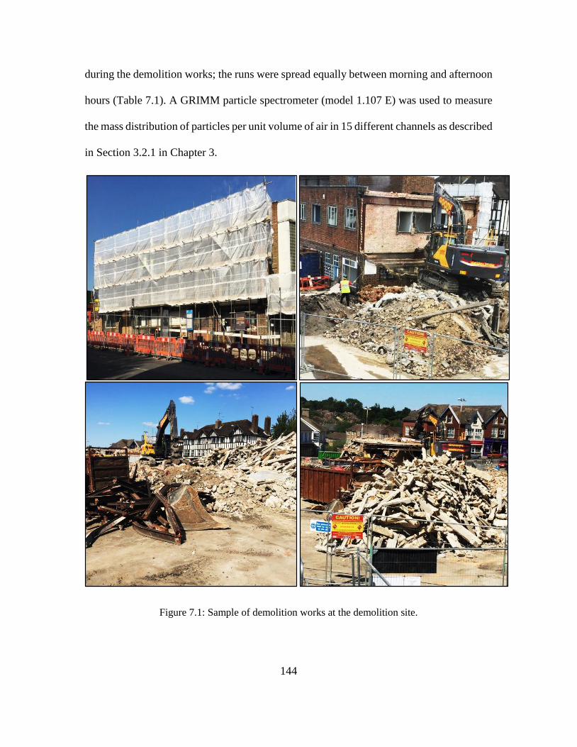
144
during the demolition works; the runs were spread equally between morning and afternoon
hours (Table 7.1). A GRIMM particle spectrometer (model 1.107 E) was used to measure
the mass distribution of particles per unit volume of air in 15 different channels as described
in Section 3.2.1 in Chapter 3.
Figure 7.1: Sample of demolition works at the demolition site.

145
Table 7.1: Description of sampling duration and monitoring sites.
Day
number
Date Start-end time
(sampling duration
in minutes)
Measurement
type
Measurement location
with respect to
demolition site (x)
1 28 June
2015
10:00:00–14:00:00
(~240)
Background At 15 m downwind
of demolition site
2, 3 1, 3 July
2015
08:56:01–17:00:07
(~500)
08:33:01–16:56:37
(~500)
Fixed-site At 10 m downwind of
the demolition site
4, 5 6, 8 July
2015
08:46:01–17:01:13
(~500)
08:35:01–16:59:25
(~500)
Mobile
measurements
Around the demolition
site in ~100 m (route
A) and ~600 m (route
B) loop
6, 7 9, 10 July
2015
14:12:01–16:46:43
(~150)
08:39:01–16:44:01
(~500)
Sequential
measurements
At 10, 20, 40 and 80 m
downwind of
demolition site
7 10 July
2015
11:03:00–14:40:00
(~220)
Excavator cabin At 5 m downwind
inside the vehicle
cabin
2, 3, 4, 6, 7 1, 3, 6, 9, 10
July 2015
15:10:00–15:49:00
(~40)
13:25:00–14:00:00
(~35)
14:30:00–15:00:00
(~30)
14:10:00–14:40:00
(~30)
15:00:00–15:10:00
(~10)
Engineer’s on-
site office
At 16 m downwind
inside the office

146
Figure 7.2: Schematic map of the experimental set-up, showing (a, b) monitoring stations around
the demolition site (DS) during (c) fixed site measurements at day 2, and (d) day 3. Route of mobile
measurements around the DS during (e) day 4, and (f) day 5. SP and EP refer to the start and end
points, respectively, while the arrows represent the path of mobile measurements.
DSDS
(c) Fixed-site (day 2) (d) Fixed-site (day 3)
(e) Mobile route A (day 4)
(g) Sequential measurements (day 6) (h) Sequential measurements (day 7)
DS
DS DS1
2
34
1
2
34
DS
DS
Demolition site
(a) Location area (b) Site Location
10 m
10 m
Route loop : ~100 m Route loop :~ 600 m
SP/EP
Wind direction
Wind direction Wind direction
Wind direction
Wind directionWind direction
SP/EP
(f) Mobile route B (day 5)

147
Figure 7.3: Wind roses diagrams depict the hourly frequency distribution of the wind speed and
direction during the fixed site measurement on day 2 (a) and day 3 (b), as well as during the mobile
measurements on day 4 (c) and day 5 (d), for sequential distances at day 6 (e) and day 7 (f).
7.2.2 Collection of PM mass on PTFE filters for SEM and EDS analysis
Five different samples (1-5) were collected on PTFE filters that had a diameter of
47 mm and a nominal thickness of ~1000 µg cm-2 (Table 7.2). Filter sample 1 was treated
as a “blank” while mass on sample 2 was collected during the background period (pre-
demolition). Mass on filter samples 3, 4 and 5 were collected during fixed-site (days 2 and
3), mobile (days 4 and 5) and sequential measurements (days 6 and 7), respectively. Further
details on the sampling duration and mass collected on the sampled filters are provided in
Table 7.2. Each of these five filter samples were analysed using a JEOL SEM (model: JSM-
Frequency of counts by wind direction (%)
W
S
N
E10%
20%
30%
40%50%
60%70%
80%
90%100%
110%
mean = 10.1
calm = 0%
2015
0 to 2 2 to 4 4 to 66 to 13
(m s1)
Frequency of counts by wind direction (%)
W
S
N
E
5%
10%
15%
20%
25%
30%
35%
40%
45%
50%
mean = 6.04
calm = 0%
0 to 2 2 to 4 4 to 6 6 to 9
(m s1)
Frequency of counts by wind direction (%)
W
S
N
E
10%
20%
30%
40%
50%
60%
70%
80%
90%
mean = 5.62
calm = 0%
0 to 2 2 to 4 4 to 6 6 to 9
(m s1)
Frequency of counts by wind direction (%)
W
S
N
E
20%
40%
60%
80%
100%
120%
mean = 6.62
calm = 0%
0 to 2 2 to 4 4 to 6 6 to 10
(m s1)
Frequency of counts by wind direction (%)
W
S
N
E
10%
20%
30%
40%
50%
60%
mean = 5.83
calm = 0%
0 to 2 2 to 4 4 to 6 6 to 11
(m s1)
Frequency of counts by wind direction (%)
W
S
N
E
10%
20%
30%
40%
50%
60%
70%
80%
90%
100%
110%
mean = 10.2
calm = 0%
0 to 2 2 to 4 4 to 6 6 to 14
(m s1)
(a) Fixed-site
(day 2)(b) Fixed-site
(day 3)
(c) Mobile route
(day 4)
(e) Different distances
(day 6)
(f) Different distances
(day 7)(d) Mobile route
(day 5)
Frequency of counts by wind direction (%)
W
S
N
E
5%
10%
15%
20%
25%
30%
35%
40%
45%
50%
mean = 6.04
calm = 0%
0 to 2 2 to 4 4 to 6 6 to 9
(m s1)
mean:3.00 0.83 m s-1 mean:3.00 1.49 m s-1mean:3.00 1.94 m s-1
mean:4.00 1.12 m s-1 mean:2.00 0.73 m s-1 mean:2.00 1.48 m s-1
m s–1
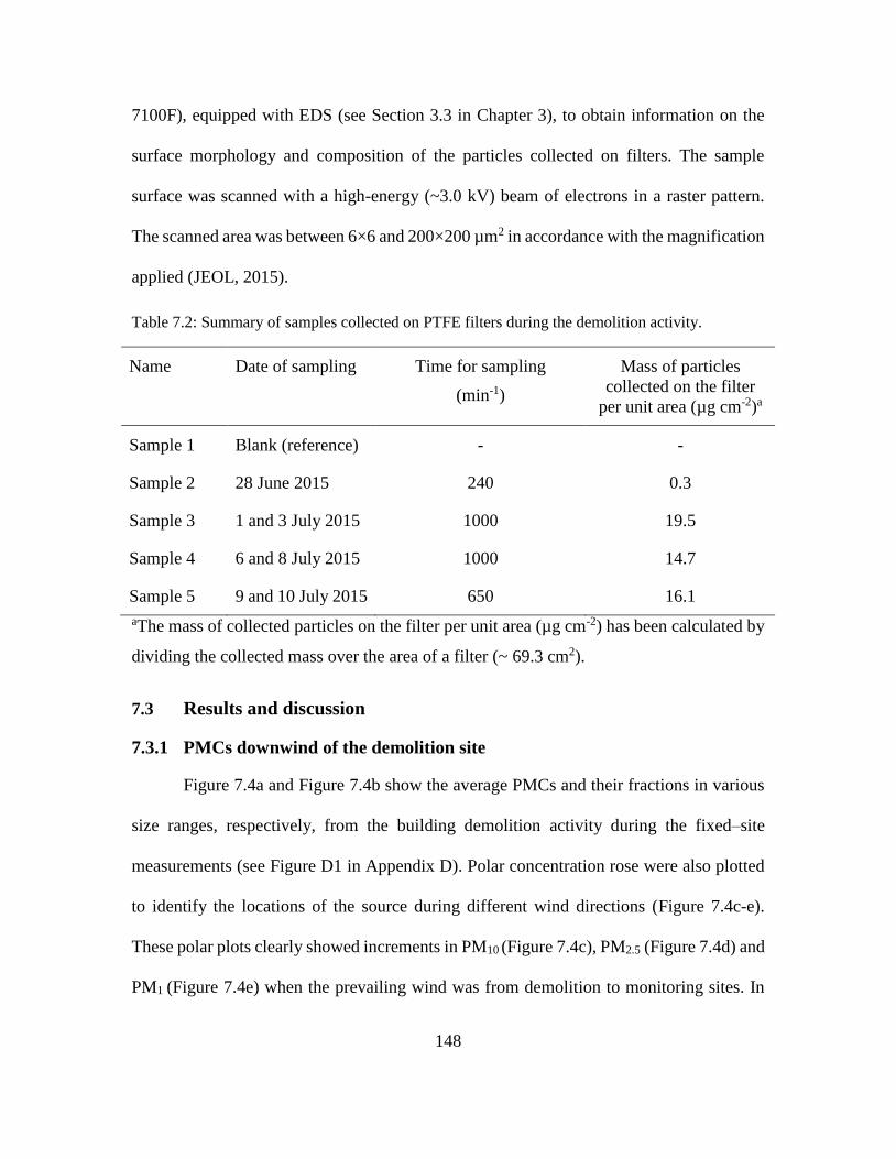
148
7100F), equipped with EDS (see Section 3.3 in Chapter 3), to obtain information on the
surface morphology and composition of the particles collected on filters. The sample
surface was scanned with a high-energy (~3.0 kV) beam of electrons in a raster pattern.
The scanned area was between 6×6 and 200×200 µm2 in accordance with the magnification
applied (JEOL, 2015).
Table 7.2: Summary of samples collected on PTFE filters during the demolition activity.
Name Date of sampling Time for sampling
(min-1)
Mass of particles
collected on the filter
per unit area (µg cm-2)a
Sample 1 Blank (reference) - -
Sample 2 28 June 2015 240 0.3
Sample 3 1 and 3 July 2015 1000 19.5
Sample 4 6 and 8 July 2015 1000 14.7
Sample 5 9 and 10 July 2015 650 16.1
aThe mass of collected particles on the filter per unit area (µg cm-2) has been calculated by
dividing the collected mass over the area of a filter (~ 69.3 cm2).
7.3 Results and discussion
7.3.1 PMCs downwind of the demolition site
Figure 7.4a and Figure 7.4b show the average PMCs and their fractions in various
size ranges, respectively, from the building demolition activity during the fixed–site
measurements (see Figure D1 in Appendix D). Polar concentration rose were also plotted
to identify the locations of the source during different wind directions (Figure 7.4c-e).
These polar plots clearly showed increments in PM10 (Figure 7.4c), PM2.5 (Figure 7.4d) and
PM1 (Figure 7.4e) when the prevailing wind was from demolition to monitoring sites. In

149
fact, the overall average of PM10, PM2.5 and PM1 concentrations were found to be
133.1±17.2 μg m−3, 15.0±6.3 μg m−3 and 7.9±5.2 μg m−3, with a fraction of about 89, 5 and
6% in PM2.5-10, PM1-2.5 and PM1 size ranges, respectively (Section D2 in Appendix D).
Fraction of coarse particles (i.e. PM2.5-10) was found to be about 39% higher over the
background level, compared with fine particles (i.e. PM2.5) that reduced by about similar
percentage, against the background level during the demolition periods. This observation
clearly suggests a much higher increase of coarse particle emissions from building
demolition (Figure 7.4).
As far as the regulatory metrics are concerned, the average concentrations of PM10, PM2.5
and PM1 were found to be up to 11-times higher during the demolition periods than the
background levels of PM10 (12.0±6.3 µg m–3), PM2.5 (6.07±2.6 µg m–3) and PM1 (2.0±1.1
µg m–3; Figure 7.3a). Published studies on this topic are limited for direct comparison but
results of this study were analogous to that observed by previous studies. For example,
Dorevitch et al. (2006) measured PM10 during the demolition of a brick-walled reinforced
concrete building and average concentrations were reported to be up to 10-times higher
compared with background levels. Later, Hansen et al. (2008) measured PM1 particles from
the demolition of a brick-walled concrete building and found about 3-fold increase in
concentration during the demolition over the background values. The differences in peak
concentrations with respect to the background levels changed drastically. For example, the
peak values of PM10, PM2.5 and PM1 during the demolition period increased to about 7358,
348 and 42 μg m−3, which were 615-, 60- and 30-times higher than the background levels,
respectively. Closer inspection of the log-sheets indicated these peak increments to be

150
coinciding with the periods of intense breaking of the ceiling and side walls at the upper
floors of the demolished building (Figure 7.4).
Figure 7.4: (a) The average concentrations of PM10, PM2.5 and PM1 with average of prevailing wind
direction, during all days of fixed site measurements. The inner and outer circles represent fractions
of PMCs in various size range.
0
50
100
150
200
250
PM10 PM2.5 PM1
Average wind speed: 3 (m s-1)
PM
10;
PM
2.5
; P
M 1
(µg m
-3)
(b)
(c) (d)
(a)
(e)0
20
40
60
80
100
120
140
PM10 PM2.5 PM1
Activity Background
50%33%
17%
89%
5%
6%
PM 2.5-10
PM1-2.5
PM1
PM
10;
PM
2.5
(µg m
-3)
PM
1 (µ
g m
-3)
0
0.2
0.4
0.6
0.8
0
2
4
6
8
0 1000 2000 3000 4000 5000 6000 7000 8000 9000 10000
Hu
nd
red
s
PM10
PM2.5
PM1
PM1PM2.5PM10
8:00 10:00 14:0012:00 16:00
Time
8:00 10:00 14:0012:00 16:00
(f) Fixed-site (day 2) Fixed-site (day 3)
103 10 3
151
Histograms of PM10, PM2.5 and PM1 concentration were made using the SPSS statistical
software for comparing measured concentrations against the air quality standards (SI
Figure D2). The EU Directive 2008/50/EC (Directive, 2008) and WHO guidelines (WHO,
2006) suggest the daily mean concentrations of PM10 and PM2.5, not to exceed of 50 µg m-
3 (on more than 35 occasions per year) and 25 µg m-3, respectively. The results showed that
a cumulative percentage of concentrations for about 42% exceeded the EU daily limit value
for PM10 and about 11% of the time the daily mean WHO limits of PM2.5.
The above observations clearly suggest increased concentrations above the background and
exceedances over the regulatory limits, especially for daily mean PM10, for over 2/3rd of
total demolition period. On the other hand, the exceedances of PM2.5 were minimal,
indicating that more efficient preventive measures (e.g. wind barriers, building sealing by
impermeable plastic foil or water spraying (Kumar et al., 2012b) is needed to contain the
PM10 emissions within the site boundaries in order to decrease the exposure to public in
the downwind of such sites.
7.3.2 Spatial variations of PM during mobile measurements
In order to understand the exposure to people around the demolition site, the spatial
variation of PM10, PM2.5 and PM1 concentrations were assessed on the routes A and B that
have a closed “mobile monitoring” loop of about 100 and 600 m, respectively, around the
demolition site. The average PM10, PM2.5 and PM1 for the route A were measured as
162.7±48.4, 15.5±0.8 and 4.7±1.2 μg m−3 (Figure 7.5a), respectively, with about 4- and
two-times lower PM10 (37.2±9.1 μg m−3) and PM2.5 (7.5±3.6 μg m−3) and slight decrease
in PM1 (3.5±1.0 μg m−3) at the route B (Figure 7.5b). Fractions of coarse (and fine) particles
152
were found about 90% (10%) and 79% (21%) at route A and route B, respectively (see
Figure D3). The higher PMC and fraction of coarse particles at the route A was expected,
given that this route was around the periphery of the site compared with route B which was
further apart from the demolition site (Table 7.3).
The increase in PMC during the mobile measurements cannot be directly attributed to the
demolition activity since the collected data also included the periods when the mobile
sampling location was in the upwind of the routes A and B. Therefore, to separate the
upwind (primarily baseline, or background, PM concentrations arriving at the site) and
downwind concentrations (primarily baseline plus the contribution from the building
demolition), firstly the spatially averaged PM concentrations (Figure 7.6) were plotted and
then divided the upwind and downwind data set to identify contribution from the
demolition activity.
For both routes, the PMCs were much higher in downwind than those in upwind of the site
and these differences were highest for the PM10, followed by PM2.5 and PM1. For example,
the average PM10 PM2.5 and PM1 in downwind (217.4, 21.0 and 6.6 μg m−3) were about
7.7, 2.3 and 2.1 times higher than those in upwind (28.3, 9.3 and 3.1 μg m−3) areas of the
demolition site on the route A; with corresponding values on the route B being 63.6, 12.3
and 4.7 μg m−3 (in downwind) and 21.0, 3.1 and 2.0 μg m−3 (in upwind).
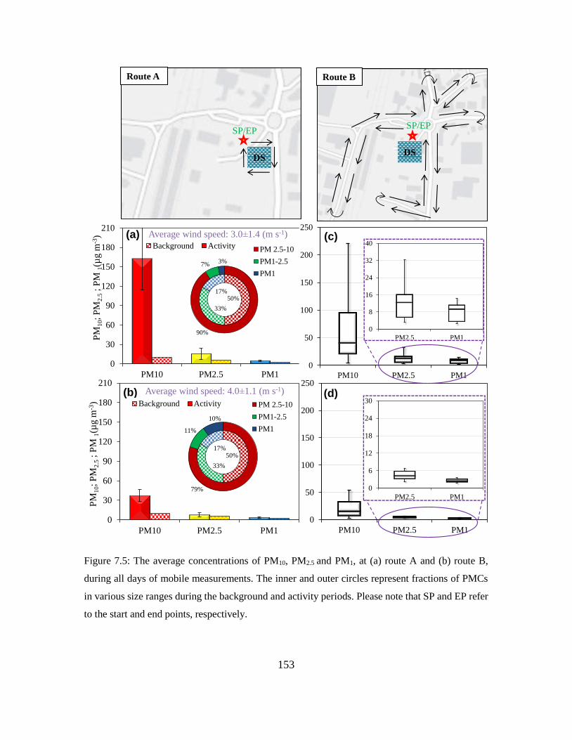
153
Figure 7.5: The average concentrations of PM10, PM2.5 and PM1, at (a) route A and (b) route B,
during all days of mobile measurements. The inner and outer circles represent fractions of PMCs
in various size ranges during the background and activity periods. Please note that SP and EP refer
to the start and end points, respectively.
0
50
100
150
200
250
PM10 PM2.5 PM1
0
30
60
90
120
150
180
210
PM10 PM2.5 PM1
0
30
60
90
120
150
180
210
PM10 PM2.5 PM10
50
100
150
200
250
PM10 PM2.5 PM1
PM
10;
PM
2.5
; P
M 1
(µg m
-3) (a)
(b)
Average wind speed: 3.0±1.4 (m s-1)
Average wind speed: 4.0±1.1 (m s-1)
PM
10;
PM
2.5
; P
M 1
(µg m
-3)
(c)
(d)
Route A
DSDS
Route B
0
8
16
24
32
40
PM2.5 PM1
0
5
10
15
20
25
30
35
40
45
50
Background Activity
Background Activity
0
5
10
15
20
25
30
35
40
45
50
Background Activity
Background Activity
50%
33%
17%
79%
11%
10%
50%
33%
17%
90%
7%3%
PM 2.5-10
PM1-2.5
PM1
PM 2.5-10
PM1-2.5
PM1
0
6
12
18
24
30
PM2.5 PM1
SP/EPSP/EP
154
Peak concentrations are usually reflection of the intense emission activities, which reached
to 3510.9 (PM10), 244.5 (PM2.5) and 31.2 μg m−3 (PM1) which were 16.2, 11.6 and 4.7-
times over the average PMCs on the downwind of the route A. The manual log of activities
showed these peak PMCs corresponding to intense breaking of reinforced concrete beams
and shifting the waste material from the site that may have led to generation and
resuspension of particles from the site. It was clear from the results that the close vicinity
(route A) of the demolition site in downwind wind direction was significantly more
influenced by PM emissions and that the most influenced size range was PM10.
It will be interesting to put measurements of this study in the context of relevant mobile
measurement studies. For example, Gulliver and Briggs (2004) reported results on
variation of PM10 concentration during walking on the suburban routes in Northampton,
UK. Their average PM10 concentrations (38.1±25.1 μg m−3) were ∼6 and 2-times lower
than those found in downwind of routes A and B of this study, respectively. Furthermore,
Kaur et al. (2005) found the average concentration of PM2.5 to be 27.5 μg m−3 during the
measurement of pedestrian exposure during walk along a major road in London (UK)
which was slightly higher (~1.3) than averaged downwind PM2.5 of this work (21.0 μg
m−3). The measured downwind PM2.5 on the route A were about 3-times higher than those
found inside the car (6.60 μg m−3) by Weichenthal et al. (2014) in Toronto (Canada).
This is clear from the above contextualisation that while PM10 concentrations can be much
higher in the downwind of demolition sites compared to those the most polluted roadside
environments in urban areas; the PM2.5 emissions from demolition are generally less
pronounced and comparable to urban walking and in-vehicle studies.

155
Figure 7.6: The spatially averaged concentrations of PM10, PM2.5 and PM1 during mobile
measurements at (a) route A and (b) route B. The words Avg, DW and UW in the figure represent
average, downwind and upwind, respectively. A number of parallel points at each route were due
to the sensitivity of GPS device, which varied within ±3.5 m at the same route.
Route BRoute A
DS
DS
SP/EP
DS
DS
DS
DS
Avg wind direction = 200o±30o
Avg wind direction
= 280o±29o
Avg wind direction
= 280o±29o
Avg wind direction
= 280o±29oAvg wind direction = 200o±30o
Avg wind direction = 200o±30o
UW DW
PM2.5–10 (%): 67 90
PM10 (μg.m−3): 28 217
UW DW
PM1–2.5 (%): 22 7
PM2.5 (μg m−3): 9 21
UW DW
PM1 (%): 11 3
PM1 (μg m−3): 3 6
UW DW
PM2.5–10 (%): 85 81
PM10 (μg.m−3): 21 63
UW DW
PM1–2.5 (%): 5 12
PM2.5 (μg m−3): 3 12
UW DW
PM1 (%): 10 7
PM1 (μg m−3): 2 4
PM10
PM2.5
PM1
(μg m−3)
(μg m−3)
(μg m−3)
(μg m−3)
(μg m−3)
(μg m−3)
SP/EP
SP/EP
SP/EP
SP/EP
SP/EP

156
Table 7.3: PM10, PM2.5 and PM1 concentrations (µg m-3) during mobile measurements at routes A
and B.
Route A Route B
PM10 PM2.5 PM1 PM10 PM2.5 PM1
Run 1A 48.8±20.7 12.2±2.1 4.3±0.6 Run 1B 35.0±5.1 12.2±0.5 4.7±0.4
Run 2A 29.6±2.7 9.8±0.1 3.9±0.2 Run 2B 28.4±7.8 9.1±1.3 3.9±0.7
Run 3A 133.9±83.5 19.4±5.3 8.3±1.3 Run 3B 61.7±56.8 12.2±5.2 4.9±1.2
Run 4A 202.4±198.0 19.9±12.1 5.8±1.3 Run 4B 32.9±9.6 9.3±1.6 4.5±1.1
Run 5A 331.7±204.1 27.0±9.3 6.7±1.0 Run 5B 75.8±81.3 10.5±6.3 3.5±1.7
Run 6A 24.4±6.6 8.3±1.6 4.2±1.3 Run 6B 28.2±20.4 7.4±1.1 4.0±0.9
Run 7A 53.3±37.1 7.0±4.5 2.2±0.4 Run 7B 23.5±11.6 4.6±0.7 2.7±0.8
Run 8A 440.1±358.5 30.9±24.3 5.2±2.2 Run 8B 29.9±37.6 5.0±1.2 3.1±0.4
Run 9A 171.4±96.8 13.5±4.5 4.1±0.6 Run 9B 25.3±15.6 5.5±0.4 3.2±0.6
Run 10A 155.5±91.7 12.9±1.9 4.4±0.9 Run 10B 58.2±54.5 6.4±3.2 2.7±0.6
Run 11A 150.8±56.8 11.4±1.7 3.5±0.3 Run 11B 29.5±22.9 5.1±1.2 3.0±0.4
Run 12A 210.8±114.4 13.8±4.7 3.4±0.8 Run 12B 17.9±8.7 3.3±0.4 2.2±0.2
Overall
average
162.7±48.4 15.5±0.8 4.7±1.2 Total 37.2±9.1 7.5±3.6 3.5±1.0
7.3.3 Concentrations inside the excavator cabin and temporary on-site office
Excavator vehicle and on-site temporary offices are integral part of demolition sites
where drivers and on-site workers remain present. In order to understand how the
concentration levels change during the demolition periods in these settings, the
measurements made showed the average (and peak) concentrations of PM10, PM2.5 and
PM1 inside the excavator cabin as 455±349 (54124), 109±54 (12401) and 75±14 (699) μg

157
m−3, respectively (Figure 7.7a), which were about 38 (4500), 18 (2060) and 37 (350) times
higher than those during the background periods, respectively. These relatively higher
average concentrations and the notably high peak values inside the excavator cabin,
compared with fixed-site (Section 7.3.1) and mobile measurements (Section 7.3.2), were
expected due to a very close proximity (~5 m) of the excavator cabin from the demolition
site.
Figure 7.7: The concentrations of PM10, PM2.5 and PM1, at (a) the excavator cabin and (b) temporary
on-site office for site engineers and managers during the background and working periods,
respectively.
0 250 500 750 1000
PM 10
PM2.5
PM1
Sampling points
PM
10
, P
M2
.5 ,
PM
1(µ
g m
–3)
0 50 100 150 200
PM10
PM2.5
PM1
Excavator
Temporary on-site office for site engineers
(a)
(b)
Average wind speed = 3.6 ms-1
PM
10
, P
M2
.5 ,
PM
1(µ
g m
–3) Average wind speed = 3.7 ms-1
PM 2.5-10
PM1-2.5
PM1
PM 2.5-10
PM1-2.5
PM1
50%33%
17%
76%
7%
17%
50%33%
17%
83%
8%
9%

158
As for the concentrations in on-site temporary office, the average (and peak)
concentrations of PM10, PM2.5 and PM1 were measured as 90±4 (2566), 16±6 (341) and 8±4
(26) μg m−3 during the days of measurements, respectively (Figure 7.7b). The
corresponding average (and peak) PM10, PM2.5 and PM1 increased to 8 (214), 9 (57) and 7
(13) times higher over the background levels during the building demolition periods. These
peak values for on-site office were recorded during the time of intense demolition of the
building’s ceiling and falling of demolished materials such as brick and concrete pieces
from heights to the ground level at the site. Furthermore, a greater fraction of coarse
particles (i.e. 83%), compared to that (~76%) in excavator cabin, was found in on-site
temporary offices (Figure 7.7). This higher fraction could be expected due to much higher
ventilation, and hence penetration of particles, to the site office through windows and doors
openings as opposed to the much air tighter excavator cabin.
The above results clearly reflect that drivers of excavator vehicle and the other on-site
workers, engineers or supervisors are exposed to relatively high level of PM concentrations
at the demolition sites. The levels of concentrations, as expected, reduce with the distance
from the source (i.e. demolition site in this case) and release of emissions from demolition
activity is much larger in PM10 size fraction compared with PM2.5 (Figure 7.7).

159
7.3.4 PM decay profiles
The PM data collected at different downwind distances (i.e. at 10, 20, 40 and 80 m)
was plotted for evaluating the horizontal decay in concentrations of PM10, PM2.5 and PM1
in the downwind of demolition site (Figure 7.8). In order to find the best fit function, both
the logarithmic (Figure 7.8) and exponential (see Figure D4) best fit functions were applied
to net ΔPM10, ΔPM2.5 and ΔPM1 concentrations, which were determined by subtracting the
background PMCs from the measured concentrations during the demolition period. The
ΔPM concentrations at downwind distances showed a negatively correlated logarithmic
form (Figure 7.8), with R2 values as 0.94 (ΔPM10), 0.93 (ΔPM2.5) and 0.84 (ΔPM1). For the
discussion purposes, the logarithmic decay function (Figure 7.8) was chosen as a best fit to
the data due to better R2 values than those given by an exponential decay profile as 0.85,
0.89 and 0.68 for ΔPM10, ΔPM2.5 and ΔPM1), respectively (see Figure D4).
The decay profiles suggest a higher rate of change in PM concentrations close to the
demolition site compared with those at farther distances. For example, the rate of change
in ΔPM10, ΔPM2.5 and ΔPM1 concentration with per meter distance are (1.60, 0.51, 0.27)
μg m-3 between 10 and 20 m, which decreases to (0.27, 0.45, 0.04) and (0.19, 0.06, 0.01)
μg m-3 per meter distance in the 20-40 m, and 40-80 m range, respectively (Figure 7.8).
Furthermore, the average PM10, PM2.5 and PM1 concentrations reached to half of their
initial concentrations within 80, 50 and 50 m from the demolition site, respectively
(Figure 7.8).

160
Figure 7.8: (a) Horizontal decay profiles of ΔPM10, (b) ΔPM2.5 and (c) ΔPM1 at the demolition site
during the sequential measurements; x and y expresses distance from the demolition site and ΔPM
values, respectively.
y = -1.77ln(x) + 11.59 (R² = 0.84)
0
10
20
30
40
50
0 20 40 60 80 100
y = -8.51ln(x) + 40.60 (R² = 0.93)
0
20
40
60
80
100
0 20 40 60 80 100
y = -13.57ln(x) + 92.57 (R² = 0.94)
0
20
40
60
80
100
0 20 40 60 80 100
ΔP
M1
0 (µ
g m
-3)
(b)
(c)
(a)
y = -12.02ln(x) + 85.67 (R² = 0.85)
y = -2.45ln(x) + 19.33 (R² = 0.93)
y = -2.11ln(x) + 14.20 (R² = 0.84)
0
20
40
60
80
100
0 20 40 60 80 100
PM10
PM2.5
PM1
Log. (PM10)
Log. (PM2.5)
Log. (PM1)
y = -12.02ln(x) + 85.67 (R² = 0.85)
y = -2.45ln(x) + 19.33 (R² = 0.93)
y = -2.11ln(x) + 14.20 (R² = 0.84)
0
20
40
60
80
100
0 20 40 60 80 100
PM10
PM2.5
PM1
Log. (PM10)
Log. (PM2.5)
Log. (PM1)
y = -12.02ln(x) + 85.67 (R² = 0.85)
y = -2.45ln(x) + 19.33 (R² = 0.93)
y = -2.11ln(x) + 14.20 (R² = 0.84)
0
20
40
60
80
100
0 20 40 60 80 100
PM10
PM2.5
PM1
Log. (PM10)
Log. (PM2.5)
Log. (PM1)
y = -15.13ln(x) + 123.52 (R² = 0.94)
y = -14.57ln(x) + 74.02 (R² = 0.92)
y = -1.44ln(x) + 13.06 (R² = 0.83)
0
20
40
60
80
100
0 20 40 60 80 100
PM10
PM2.5
PM1
Log. (PM10)
Log. (PM2.5)
Log. (PM1)
y = -15.13ln(x) + 123.52 (R² = 0.94)
y = -14.57ln(x) + 74.02 (R² = 0.92)
y = -1.44ln(x) + 13.06 (R² = 0.83)
0
20
40
60
80
100
0 20 40 60 80 100
PM10
PM2.5
PM1
Log. (PM10)
Log. (PM2.5)
Log. (PM1)
y = -15.13ln(x) + 123.52 (R² = 0.94)
y = -14.57ln(x) + 74.02 (R² = 0.92)
y = -1.44ln(x) + 13.06 (R² = 0.83)
0
20
40
60
80
100
0 20 40 60 80 100
PM10
PM2.5
PM1
Log. (PM10)
Log. (PM2.5)
Log. (PM1)
ΔP
M2
.5 (µ
g m
-3)
ΔP
M1
(µg m
-3)
Distance (m)
50% of initial concentration
50% of initial concentration
50% of initial concentration
161
Similar decay profiles from demolition works are not available for comparison but other
studies for construction or roadside (Buonanno et al., 2009; Hagler et al., 2009; Hitchins et
al., 2000) have either logarithmic or exponential decay profiles. For example, Azarmi et al.
(2015b) and Buonanno et al. (2009) found the decay profiles of PM10 and PM2.5 for the
construction works in London (UK) and at the highway in Cassino (Italy) as logarithmic
and exponential, respectively.
In order to understand how far the initial concentrations from demolition site reaches to
meet the standard limits, the daily limits of the EU Directive 2008/50/EC (Directive, 2008)
for PM10 and WHO guidelines for PM2.5 (WHO, 2006) were compared with decaying
concentrations of this study (Section D3 in Appendix D). PM10 and PM2.5 took 50 and 15
m in the downwind of demolition site to meet the EU and WHO daily mean standard values,
respectively (see Figure D5). This distance could be taken as a public exclusion zone in the
downwind direction of such demolition sites during demolition days.
7.3.5 The PMEFs for building demolition
Using the modified box model described in Section 3.4.2 and the PM data
monitored downwind of the building demolition at the fixed-site (Section 7.3.1), the
average PMEFs for PM10, PM2.5 and PM1 were estimated as 35±1, 17±4 and 4±0.5 µg m–2
s–1, respectively (see Table D2). While there are numerous field studies available for
emission factors from road traffic (Kumar et al., 2011b), limited studies are available for
road works (Font et al., 2014) and almost none for building demolition activity. For
example, Font et al. (2014) estimated emission factors for PM10 from road works in London
as 0.0022 kg m−2 month−1 which was about 6-fold smaller than those observed

162
(0.013±0.004 kg m− 2 month−1) in this study (Section D4). This difference clearly suggest
much larger emissions of PM10 during building demolition, which is expected given its dry
and intense nature compared with less intense construction activities in relatively open
areas such around roads. Results of this study were about 19-fold higher than those reported
in the UK National Atmospheric Emissions Inventory (NAEI) for the PM10 as 0.0007 kg
m−2 month−1 (NAEI, 2013) and about 2-fold greater than European emission inventory
median value (0.0068 kg m−2 month−1) (EMEP-EEA., 2013) for the demolition and
construction activities (see Figure D6). The PMEF of PM2.5 and PM1 from demolition,
construction or road works are currently unavailable and hence estimates of this wok
provide hitherto missing information for future experimental and modelling studies.
7.3.6 Morphology and chemical characterisation
SEM and EDS analyses were performed on the bulk mass of particles collected on
the filters (Table 7.4) for assessing their shape, size, composition and structure (Section
D5). Figure 7.9 shows the SEM images of the samples, indicating a heterogeneous structure
with crystal and aggregated shaped particles during the demolition works; the irregular
shaped holes show the porosity of PTFE filters. EDS analysis suggested the dominance of
silicon, Si (10.5-17.8%) and aluminium, Al (4.2-5.1%; Table 7.4).
The crystal shaped particles are thought to be Si released from concrete debris (Srivastava
et al., 2009) while the aggregated shaped particles shows the presence of metals such as Al
(Falkovich et al., 2001). The EDS analysis also showed the presence of other elemental
species (Table 7.4), with a strong peak for carbon (C) and fluorine (F) in the blank
“reference” filter, with an additional peak of nitrogen (N) in the background sample (see

163
Figure D7). C and F are thought to be the material of PTFE filters while presence of N in
the background filter is possibly from the regional background in a nitrate form due to
secondary gas-to-particle aerosol formation (Schaap et al., 2004; Viana et al., 2008). The
differences between particles deposited on the reference (sample 1) and background
(sample 2) filters and those collected during the demolition activity periods (samples 3, 4
and 5) signify the presence of new elements (Figure 7.9). Apart from the dominating
fraction of Si and Al, the additional elements during the demolition periods were found to
be sulphur (S), chlorine (Cl), magnesium (Mg), sodium (Na) and Zinc (Zn), as shown in
Table 7.4. The potential sources of these elements in urban environments are summarised
in Table D3.
Some of the deposited elements could be in oxide form because of presence of O during
the demolition activities. The increment in the intensity and ratio of O peak compared with
other peaks like Si, Al and S suggested that these elements appear to be strongly related
with building demolition sources where aluminium oxide, sulphur oxide and silicon
dioxide compounds are expected to be formed. The main source of Si is likely to be
building related activities, particularly those involving concrete material such as breaking
concrete slabs, which is typically made of cement, admixtures, water and aggregates
(Kumar and Morawska, 2014). Si can be found in asbestos-containing hazardous building
materials and it is also one of the key constituents of cement in the form of celite
(tetracalcium aluminoferrite), belite (dicalcium silicate) and alite (tricalcium silicate) (Beck
et al., 2003; Lioy et al., 2002). Al were thought of coming from breaking and demolition
of aluminium windows, steel beams and concrete since alumina (Al2O3) is integral

164
component of cement (Azarmi et al., 2015b). There are sources such as sea salt and fuel oil
fly ash for S (see Table D3) but this is expected to be predominantly arising from diesel
exhaust emissions from the construction machinery (Dorado et al., 2003). Furthermore, Na
and Cl were mostly likely due to the effect of sea salt brought by the south-westerly winds
to the site (Figure 7.3). Zn and Mg were expected to be contributed by on-site exhaust
emissions from construction machinery and soil dust, respectively. The above results
reflect the dominance of Si and Al in particles and the ability of building demolition works
to effectively aerosolise both friable and non-friable building materials to the surrounding
environment.
Table 7.4: The elemental composition of the all the filters (quantitative EDS analyses).
Sample 1
(Reference)
Sample 2
(Background)
Sample 3
(Fixed site)
Sample 4 (Mobile
measurements)
Sample 5
(Different distances)
Name Fraction
(%)
Name Fraction
(%)
Name Fraction
(%)
Name Fraction
(%)
Name Fraction
(%)
C 30.6 C 46.2 C 16.7 C 19.3 C 21.0
- - O 24.3 O 48.5 O 48.9 O 22.9
F 69.3 - - F 3.5 F 1.4 F 40.8
- - - - Si 17.8 Si 14.0 Si 10.5
- - S 1.2 S 2.3 S 4.2 - -
- - - - Al 5.1 Al 4.5 Al 4.2
- - - - Mg 1.4 Mg 2.6 Mg 0.3
- - Cl 4.4 Cl 1.9 Cl 1.5 - -
- - Na 2.6 Na 2.5 - - - -
- - N 21.0 - - - - - -
- - - - - - Zn 3.1 - -

165
Figure 7.9: SEM images of the surface morphology of the particles collected on blank filter,
background measurements, sample 3, sample 4 and sample 5 at ×50, ×1000 and ×8000 resolution.
Sam
ple
1 (
Ref
eren
ce)
Sam
ple
2 (
Bac
kgro
und)
Sam
ple
3S
ample
4S
ample
5
50 1000 8000 Dom
inan
t elemen
ts: C,F
Dom
inan
t elemen
ts: Si,A
l, S (d
emolitio
n p
eriod)
Dom
inan
t elemen
ts: C,
O
100 µm 10 µm 1 µm
100 µm 10 µm 1 µm
100 µm 10 µm 1 µm
100 µm 10 µm 1 µm
100 µm 10 µm 1 µm

166
7.3.7 Exposure to demolition workers and engineers
The average respiratory deposited doses (RDD) of coarse and fine particles were
estimated using the methodology described in Section 3.5.2 for people on and around the
demolition sites (i.e. workers, individuals around the demolition site, engineers inside a
temporary on-site offices and drivers inside the excavator vehicle cabin) during heavy and
light exercise levels (Table 7.5). Compared to the local background (pre-demolition)
exposure levels, the RDD of coarse and fine particles were found to be 58- and 5-times in
the excavator vehicle cabin, respectively, which happens to be the highest exposure among
all the assessed categories. This was followed by the fixed-site “downwind” measurements
where RDD rate for coarse (and fine) particles were 20- (and 3-) times over the background,
followed by 32- (and 4-) times at the downwind of mobile measurements on the routes A
compared to only 9- (and 3-) times at the route B and 13- (and 2-) times in the on-site
temporary office (Figure 7.10). Given a logarithmic decay of emissions away from the site
(Section 7.3.4), the distance from the demolition site was an important variable to describe
the differences in RDD. For example, highest RDD were calculated at the closed locations
to the source, such as at the excavator vehicle cabin (see Figure D8). As expected,
downwind RDD of coarse (and fine) particles during mobile measurements were 10- (and
3-) times higher for route A, and 3- (and 4-) times higher for route B, respectively,
compared to those in upwind of demolition site. These downwind exposures are much
higher than those reported during walking on typical urban routes. For instance, the PM10
and PM2.5 concentrations measured by Gulliver and Briggs (2004) during walking on
suburban routes in Northampton, UK were used to calculate RDD for comparison. Their
RDD for coarse (and fine) particles were found to be up to 8- (and 2-) and 2- (and 0.8-)
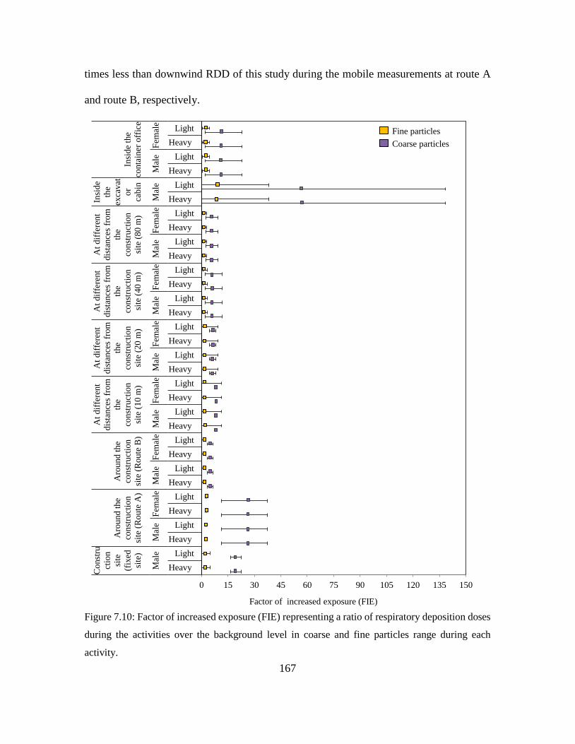
167
times less than downwind RDD of this study during the mobile measurements at route A
and route B, respectively.
Figure 7.10: Factor of increased exposure (FIE) representing a ratio of respiratory deposition doses
during the activities over the background level in coarse and fine particles range during each
activity.
0 15 30 45 60 75 90 105 120 135 150
Heavy
Light
Heavy
Light
Heavy
Light
Heavy
Light
Heavy
Light
Heavy
Light
Heavy
Light
Heavy
Light
Heavy
Light
Heavy
Light
Heavy
Light
Heavy
Light
Heavy
Light
Heavy
Light
Heavy
Light
Heavy
Light
Mal
eM
ale
Fem
ale
Mal
eF
emal
eM
ale
Fem
ale
Mal
eF
emal
eM
ale
Fem
ale
Mal
eF
emal
eM
ale
Mal
eF
emal
e
Co
nst
ru
ctio
n
site
(fix
ed
site
)
Aro
un
d t
he
con
stru
ctio
n
site
(R
ou
te A
)
Aro
un
d t
he
con
stru
ctio
n
site
(R
ou
te B
)
At
dif
fere
nt
dis
tan
ces
fro
m
the
con
stru
ctio
n
site
(1
0 m
)
At
dif
fere
nt
dis
tan
ces
fro
m
the
con
stru
ctio
n
site
(2
0 m
)
At
dif
fere
nt
dis
tan
ces
fro
m
the
con
stru
ctio
n
site
(4
0 m
)
At
dif
fere
nt
dis
tan
ces
fro
m
the
con
stru
ctio
n
site
(8
0 m
)
Insi
de
the
exca
vat
or
cab
in
Insi
de
the
con
tain
er o
ffic
eFine particles
Coarse particles
Factor of increased exposure (FIE)

168
Table 7.5: The RDD rates of coarse and fine particles.
Location Gender Exercise
level
Total RDD (µg min-1×10⁻²) ±STD
Coarse particles Fine particles
Construction site (fixed site) Male Heavy 572.8±52.7 34.7±14.6
Light 290.0±26.6 17.5±7.4
Around the construction site
(route A)
Male Heavy 956.0±231.8 64.8±2.5
Light 484.1±117.3 32.8±1.2
Female Heavy 827.6±200.6 56.1±2.2
Light 383.4±92.9 26.0±1.0
Around the construction site
(route B )
Male Heavy 249.7±26.8 38.0±11.2
Light 126.4±13.5 19.2±5.6
Female Heavy 216.1±23.2 32.9±9.7
Light 100.1±10.7 15.2±4.5
At different distances from
the construction site (10 m)
Male Heavy 238.7±4.7 39.5±26.9
Light 120.8±2.4 20.2±13.6
Female Heavy 206.6±4.1 34.2±23.3
Light 95.7±1.9 15.8±10.8
At different distances from
the construction site (20 m)
Male Heavy 185.1±34.4 32.0±22.4
Light 93.7±17.4 16.2±11.3
Female Heavy 160.3±29.8 27.7±19.4
Light 74.2±13.8 12.8±8.9
At different distances from
the construction site (40 m)
Male Heavy 202.9±84.0 18.7±4.7
Light 102.7±42.5 9.5±2.3
Female Heavy 175.3±72.7 16.2±4.0
Light 81.3±33.6 7.5±1.8
At different distances from
the construction site (80 m)
Male Heavy 175.5±60.3 15.4±4.1
Light 88.8±30.5 7.8±2.0
Female Heavy 151.9±52.2 13.3±3.5
Light 70.4±24.1 6.1±1.6
Inside the excavator cabin Male Heavy 1662.8±1422.3 78.3±38.2
Light 842.0±720.2 39.6±19.3
Inside the temporary office Male Heavy 365.4±184.3 30.7±10.9
Light 185.0±93.3 15.5±5.5
Female Heavy 316.3±159.5 26.5±9.4
Light 146.5±73.9 12.3±4.3
Background Male Heavy 29.3±17.7 15.2±6.8
Light 14.8±8.9 7.7±3.4
Female Heavy 25.3±15.3 13.1±5.9
Light 11.7±7.1 6.1±2.7

169
Result of this study also showed that exposure to coarse particle is greater compared with
fine particles due to the disproportionate increments in concentrations of coarse particles
from demolition works (Sections 7.3.1-7.3.3). Since male subjects breathe and inhale
higher doses of coarse and fine particles, compared with female subjects, due to differences
in body tidal volume and higher frequency of breathing (Section 3.7.2), male workers are
expected to inhale more particles than female workers (Figure 7.10). Furthermore, given
that breathing rate and frequency are higher during heavy exercises such as removing and
segregating demolished materials for re-use or recycling, exposure rates could vary
substantially depending on the nature of work workers are involved even if all the workers
are exposed to same emission source (see Section D6).
7.4 Chapter summary and conclusions
Size-resolved mass distributions of particles were measured in the 0.22–10 µm size
range through a combination of measurement strategies (e.g. fixed-site and mobile). The
objectives of this study were to assess emission characteristics of PM emissions in various
size ranges during the mechanical demolition of a building, in addition to understand their
physicochemical characteristics and the occupational exposure of workers to PM10, PM2.5
and PM1 on and around the demolition site.
The following conclusions are drawn:
The mass concentrations of average PM10, PM2.5 and PM1 were found to be about 11-,
3- and 4-times above the local background levels during fixed-site measurements at the
downwind of the demolition site. The coarse particles (PM2.5-10) contributed majority
(89%) of the total PMCs. The largest PM10, PM2.5 and PM1 were detected in the

170
excavator cabin during the demolition of building’s ceiling and walls.
The overall average PM10, PM2.5 and PM1 during mobile measurements at route A were
found to be 4-, 2- and 1.5-times higher than those at the route B (larger periphery of the
site), mainly due to route A being the closed periphery of the demolition site.
Segregation of the data in the downwind of the demolition site showed up to 8- and
2.5-times higher PM10 and PM2.5 concentrations than those in the upwind of the mobile
routes, respectively. These observations substantiate my previous findings that the
demolition activities produce much larger PM10 emissions compared with PM2.5. The
exposure to high PMCs can be minimised by staying indoors or being positioned
upwind of demolition sites.
ΔPM10, ΔPM2.5 and ΔPM1 values during the demolition period in the downwind
direction showed a logarithmic decay with distance (R2 ≈ 0.90). Such decay profiles are
important for extrapolating emissions in downwind of building demolition and
incorporate them in dispersion models such as were used in PMEF modelling. PM10
and PM2.5 concentrations meet the daily mean EU and WHO limit values at about 50
and 15 m, respectively, suggesting this as a public exclusion zone in this particular case.
Average emission factors during fixed-site monitoring of demolition activity were
calculated as 35.3±12.7, 12.2±3.6 and 3.9±0.5 µg m–2 s–1 for PM10, PM2.5 and PM1,
respectively. Such emission factors are currently lacking, but are key input to dispersion
models for accurately estimating the affected area around demolition sites and design
appropriate measures to limit the exposure of nearby public.

171
SEM images indicated irregular, aggregated and crystal shaped particles during the
demolition works while the EDS analysis suggested the dominance of Si and Al in the
particles. The escape of these elements along with others such as S, Zn and Mg suggest
towards appropriate protection measures of population, particularly sensitive
subgroups (e.g. elderly and children) and those in nearby sensitive areas (e.g. hospitals,
retirement home or nurseries).
The downwind distance from the demolition site was an important factor to dictate the
exposure doses. For example, highest exposure doses to coarse (and fine) particles were
found to be inside the excavator vehicle cabin, which were up to 6- (and 5-), 5- (and 3-
) and 17- (and 6-) times higher than those in downwind at the fixed-site, downwind of
the mobile route A and temporary on-site office, respectively. Other factors affecting
the exposure doses of individual workers depend on their nature of work and type of
physical exercise and therefore the RDD rates could be different to workers involved
in heavy and light exercise, site engineers or drivers even if they are exposed to same
level of particle concentrations.
This study focuses on PM10, PM2.5 and PM1 generated from the demolition of a 3-storey
brick-walled concrete building. The results showed effect of PM emissions on the exposure
to people on and around such sites. The elevated PMCs during the demolition represent a
potential health risk due to exposure to a wide variety of toxic elemental species. The
results are also important for the development of mitigation strategies prior to the
demolition operations and accordingly choose special protective equipment to limit
exposures during the demolition activities. The male subjects inhale more doses of particles

172
than female subjects, because of their higher body tidal volume and breathing frequency
and that the rate of deposited particles could considerably increase during heavy exercises
by workers for the same emission source. This suggests varying RDD rates to individual
workers depending on their nature of work. Further personal monitoring studies, focusing
on individual workers with different level of physical activities at large-scale demolition
sites, are recommended to advance the understanding of occupational exposure of on-site
workers.
173
Chapter 8. Summary, conclusions and future work
This chapter presents a summary and conclusion of this thesis drawn from the
preceding chapters. It also presents recommendations for future research.
8.1 Summary
Building works including refurbishment, construction and demolition, are now
common in both the developing and developed world. However, PM emitted from such
activities in the coarse, fine and ultrafine particle size ranges contain a wide variety of toxic
organic substances, and may adversely affect the respiratory health of on-site workers and
nearby residents (Kumar et al., 2012; Azarmi et al., 2014). This research thus set out to
conduct a series of laboratory, indoor and outdoor field measurements to determine the
impact of PM types arising from a range of building activities. The other objectives of this
thesis were to determine the emission characteristics and occupational exposure to PM10,
PM2.5, PM1 and ultrafine particles, and gain an understanding of the physicochemical
properties, of those particles such as shape, size and composition, which are currently
poorly understood. Chapter 1 outlined the background, motivation, objectives and
approach of this thesis. A comprehensive literature review of the existing knowledge and
relevant published studies of airborne PM and ultrafine particles are presented in Chapter
2. At the beginning of Chapter 2, the definitions of ultrafine particles and PM and their

174
emissions features from various building activities were also discussed. This was followed
by an assessment of the likely indoor and outdoor sources of particles, with a detailed focus
on particles derived from specific building activities. In addition, the physical and chemical
characterisations of particles were examined using physiochemical analysis such as SEM,
EDS, XPS and IBA. The review of current literature suggests that the existing knowledge
requires more extensive research to monitor the impact of building activities on the air
quality of areas surrounding building works, and to assess their potential impact and levels
of occupational exposure.
A set of experiments were set up in order to fill the research gap, as reviewed in Chapter 3,
so as to achieve the research objectives described in Chapter 1. Chapter 3 focused on the
methodologies, materials and methods which were used in the experiments, and provides
information on site descriptions and sampling set ups. The following chapters (Chapters 4-
7) presented the results obtained from the laboratory and field experiments, with a related
discussion about the measurements of particle mass, number concentrations and size
distributions. The summary of experiments, findings and conclusions were described in the
following Section 8.2 and Section 8.3 of this Chapter 8.
8.1.1 Simulated laboratory investigations
Building activities generate coarse, fine and ultrafine particles making it necessary
to understand both the exposure levels of operatives on site and the dispersion of ultrafine
particles into the surrounding environment. This study investigates the release of PM and
ultrafine particles, during the mixing of concrete (combining Portland cement with ground
granulated blastfurnace slag, GGBS or pulverised fuel ash, PFA) and the subsequent

175
drilling and cutting of hardened concrete. Particles were measured in the 5-10,000 nm size
range using a GRIMM particle spectrometer and a fast response differential mobility
spectrometer (DMS50). The mass concentrations of coarse particles contributed ~52-64%
of total mass released. The ultrafine particles dominated the total particle number
concentrations; being 74, 82, 95 and 97% for mixing with GGBS, mixing with PFA,
drilling and cutting, respectively. Peak values measured during the drilling and cutting
activities were 4 and 14 times the background. Equivalent emission factors were calculated
and the total respiratory deposition dose rates for PNCs for drilling and cutting were
32.97±9.41 ×10⁸ min−1 and 88.25±58.82 ×10⁸ min−1. These are a step towards establishing
number and mass emission inventories for particle exposure during construction activities.
8.1.2 Release of particles from indoor activities of building refurbishment
Understanding of the emissions of coarse, fine and ultrafine particles from
refurbishment activities and their dispersion into the nearby environment is of primary
importance for developing efficient risk assessment and management strategies in the
construction and demolition industry. This study investigates the release, occupational
exposure and physicochemical properties of PM and ultrafine particles, from over 20
different indoor refurbishment activities occurring at an operational building site. Particles
were measured in the 5–10,000 nm size range using a fast response differential mobility
spectrometer and a GRIMM particle spectrometer for 55 hours over 8 days. The ultrafine
particles were found to account for >90% of the total particle number concentrations and
<10% of the total mass concentrations released during the recorded activities. The highest
ultrafine particle concentrations were 4860, 740, 650 and 500 times above the background
value during wall chasing, drilling, cementing and general demolition activities,

176
respectively. Scanning electron microscopy, X-ray photoelectron spectroscopy and ion
beam analysis were used to identify physicochemical characteristics of particles and
attribute them to probable sources considering the size and the nature of the particles. The
results confirm that refurbishment activities produce significant levels (both number and
mass) of airborne particles, indicating a need to develop appropriate regulations for the
control of occupational exposure of operatives undertaking building refurbishment.
8.1.3 Assessment of PM10 and PM2.5 particles from outdoor construction
activities
Construction activities are common across cities, yet the studies assessing their
contribution to airborne PM10 and PM2.5 particles on the surrounding air quality are limited.
Here, we assessed the impact of PM10 and PM2.5 arising from outdoor construction works
in and around London. Measurements were made at 17 different monitoring stations around
three construction sites between January 2002 and December 2013. Tapered element
oscillating micro balance (TEOM 1400) and OSIRIS (2315) particle monitors were used
to measure PM10 and PM2.5 fractions in the 0.1–10 µm size range along with the ambient
meteorological data. The data were analysed using bivariate concentration polar plots and
k-means clustering techniques. Daily mean concentrations of PM10 were found to exceed
European Union target limit value of 50 µg m-3 at 11 monitoring stations but remained
within the allowable 35 exceedances per year, except at two monitoring stations. In general,
construction works found to influence downwind concentrations of PM10 relatively more
than PM2.5. Splitting of the data between working (0800-1800 h; local time) and non-
working (1800-0800 h) periods showed about 2.2-fold higher concentrations of PM10
177
during working hours compared with non-working hours. However, these observations did
not allow concluding that this increment was from the construction emissions. Together,
the polar concentration roses and the k-means cluster analysis applied to a pair of
monitoring stations across the construction sites (i.e. one in upwind and the other in
downwind) confirmed the contribution of construction sources on the measured
concentrations. Furthermore, pairing the monitoring stations in downwind of construction
sites showed a logarithmic decrease (with R2 about 0.9) in PM10 and PM2.5 concentration
with the distance. Findings of this study clearly indicate an impact of construction activities
on the nearby downwind areas and a need for developing mitigation measures to limit their
escape from the construction sites.
8.1.4 Exposure to particles from outdoor building demolition activities
Demolition of buildings produce large quantities of PM that could be inhaled by
on-site workers and people living in the neighbourhood, but studies assessing occupational
exposure at the real-world demolition sites are rare. Concentrations of PM10, PM2.5 and
PM1 were measured along with local meteorology for 54 working hours over the
demolition period. The measurements were carried out at (i) a fixed-site in the downwind
of demolished building, (ii) around the site during demolition operation through mobile
monitoring, (iii) different distances away from the demolition site through sequential
monitoring, and (iv) inside an excavator vehicle cabin and on-site temporary office for
engineers. Position of the PM instrument was continuously recorded using a Global
Positioning System on a second basis during mobile measurements. Fraction of coarse
particles contributed 89 (with mean particle mass concentration, PMC ≈ 133±17 μg m−3),

178
83 (100±29 μg m−3), and 70% (59±12 μg m−3) of total PMC during the fixed-site, mobile
monitoring and sequential measurements, respectively, compared with only 50% (mean
12±6 μg m−3) during the background measurements. The corresponding values for fine
particles (PM2.5) were 11, 17 and 30% compared with 50% during background, showing a
much greater release of coarse particles during demolition. The openair package in R and
map source software (ArcGIS) were used to assess spatial variation of PMCs in downwind
and upwind of the demolition site. A modified box model was developed to determine the
emission factors, which were 210, 73 and 24 µg m–2 s–1 for PM10, PM2.5 and PM1,
respectively. The average respiratory deposited doses to coarse (and fine) particles inside
the excavator cabin and on-site temporary office increased by 57 (and 5) and 13 (and 2)
times compared with the local background level, respectively. The monitoring stations in
downwind direction illustrated a logarithmic decrease of PM with distance. Energy-
dispersive X-ray spectroscopy and scanning electron microscopy were used to assess
physicochemical features of particles. The minerals such as silica were found as a marker
of demolition dust and elements such as sulphur coming from construction machinery
emissions. Findings of this study highlight a need to limit occupational exposure of
individuals to coarse and fine particles by enforcing effective engineering controls.
8.2 Conclusions
This thesis presents a comprehensive data set on particle mass and number
distributions and concentrations in the coarse, fine and ultrafine size ranges in the context
of building-related activities. The key conclusions obtained from the overall analysis
covered in the chapters of this thesis are summarised as follows:

179
Ultrafine particles were found to dominate the total PNCs with a proportion of 74-97%
during the laboratory simulated experiments and the indoor building refurbishment
activities, with the highest proportion of ultrafine particles arising from the cutting of
concrete, drilling and wall chasing activities. In addition, the average PNCs values were
found to be up to 38- and 84-times higher than background levels during the laboratory
simulated and indoor refurbishment activities, respectively.
The results also confirm that the simulated laboratory building activities studied here
have the potential to release PM10, PM2.5 and PM1 at levels above those encountered in
the normal background. The mechanical attrition between the surfaces of instruments
and materials during the activities and the re-suspension of existing particles appear to
be the main reasons for the production of larger-sized particles.
The highest concentrations of PM10 and PM2.5 were observed at the paired monitoring
stations during the construction works when the winds were blowing from the
construction sites toward the monitoring stations. PM10 were found about ~24, 18 and
120%, and PM2.5 were about 11% larger during the working periods compared with
those during non-working periods at the three construction sites, which can thus be
attributed to the construction works, as indicated by the bivariate concentration polar
plots and k-means clustering analysis. Moreover, the highest PM10, PM2.5 and PM1
concentrations were detected in the excavator cabin during the demolition of the
building’s ceiling and walls. This was followed by PM10, PM2.5 and PM1 concentrations
measured during downwind mobile measurements at route A (close periphery of the
demolition site), which were up to 7.7-, 2.3- and 2.1-times higher than those upwind of
the route, respectively.

180
Downwind concentrations of PM10 were found to be relatively more influenced by
construction (Chapter 6) and demolition works (Chapter 7) at the downwind of the sites
than PM2.5 concentrations. Also, the coarse particles contributed most of the total PMCs
during field construction and demolition works. Exposure to high levels of PMCs can
be minimised by staying indoors or being positioned upwind of construction and
demolition sites.
PM10, PM2.5 and PM1 values during both construction and demolition works in the
downwind direction showed a logarithmic decay relative to distance (R2 ≈ 0.90). Such
decay profiles are important for extrapolating emissions downwind of building works
to incorporate them into dispersion models such as those used in PMEF modelling. The
daily mean EU limit of value for PM10 was breached on two occasions due to
construction operations on downwind monitoring stations while measurements were
being taken between 2002 and 2013. Moreover, PM10 and PM2.5 concentrations met the
daily mean EU and WHO limit values during demolition works at about 50 and 15 m,
respectively suggesting this as a public exclusion zone in this particular case.
Average particle number and mass-based emission rates were estimated for building
simulated activities (i.e. mixing with GGBS, PFA, drilling and cutting of concrete) and
average emission factors were calculated for building demolition activity. Such
emission factors are currently lacking, but are key inputs into dispersion models for
accurately estimating the affected area around the sites and for designing appropriate
measures to limit the exposure of the nearby public.
Occupational exposures for workers on the both construction and demolition sites were
found to contribute much higher exposure over background exposure levels compared

181
with the occupational exposure for workers on indoor building works. The downwind
distance from the source was another important factor influencing exposure doses.
Other factors affecting the exposure doses of individual workers included the nature of
work and the type of physical exercise; therefore, the RDD rates could be different for
workers involved in heavy and light exercise, site engineers or drivers, even if they
were exposed to the same level of particle concentrations.
SEM images indicated irregular, aggregated and crystal shaped particles during
building refurbishment (indoor) and demolition works (outdoor). However, combining
the results of EDS, XPS and IBA analysis suggested the dominance of elements such
Si, Al, and S on the collected samples. These elements were presumably released from
the building equipment and materials (e.g. concrete, bricks and metals) involved in
refurbishment and demolition activities. The escape of these elements, along with
others such as Zn and Mg, suggests the appropriateness of protection measures for the
populace, particularly sensitive subgroups (e.g. elderly and children) and those in
nearby sensitive areas (e.g. hospitals, retirement homes or nurseries).
8.3 Recommendations for future research
This subject and area of research offers a good scope for further work to understand
the formation mechanism of particles, their dispersion behaviour and mitigation methods.
These are some recommendations that should be considered for future work:
The findings of laboratory investigations have implications both for the owners of
buildings and regulatory bodies, which appear to be unaware of the potential for indoor
building works to produce to ultrafine particles at levels significantly above a typical

182
background. Further studies covering different types of simulated building activities
with a longer time duration, are needed to better understand variations of PNCs, PMCs
and associated exposure doses.
These high levels of ultrafine particles during indoor refurbishment activities suggest
that there is a need to design more detailed and appropriate risk mitigation strategies
to limit exposure of on-site workers in indoor operation sites. It is also recommended
to perform decay profiles of PM10, PM2.5, PM1 and ultrafine particles to evaluate the
variations in PMCs and PNCs at different indoor distances, which can be used in future
dispersion modelling studies of indoor field activities. More investigations are also
needed by repeating the same experiments under varying meteorological conditions
and on different operational sites, in order to develop emission inventories for PM10,
PM2.5, PM1 and ultrafine particles.
The findings of outdoor construction measurements will enable authorities to develop
risk assessment and mitigation strategies for the construction industry. Further
research is required to monitor and understand the physicochemical properties of PM,
and also the emission levels of ultrafine particles arising from the construction works
in different meteorological conditions, to establish suitable exposure limits for on-site
workers.
In order to provide adequate protection for workers and for the populations living in
the neighborhood of outdoor demolition works, further studies, involving monitoring
of size-resolved particles from a wide variety of building demolition works within
different urban morphological and meteorological settings are recommended.
Dedicated studies are also needed in the future that can allow the PND signatures of

183
outdoor building activities to be quantified, as well as the formation pathways and
emission levels of particles in the ultrafine particles size range during different seasons
and atmospheric stability conditions.

184
References
Abbey, D.E., Ostro, B.E., Fraser, G., Vancuren, T., Burchette, R.J., 1994. Estimating fine
particulates less than 2.5 microns in aerodynamic diameter (PM2.5) from airport
visibility data in California. Journal of Exposure Analysis and Environmental
Epidemiology 5, 161-180.
Abu-Allaban, M., Gillies, J., Gertler, A., Clayton, R., Proffitt, D., 2007. Motor vehicle
contributions to ambient PM10 and PM2.5 at selected urban areas in the USA.
Environmental Monitoring and Assessment 132, 155-163.
Abu-Allaban, M., Hamasha, S., Gertler, A., 2006. Road dust resuspension in the vicinity
of limestone quarries in Jordan. Journal of the Air & Waste Management
Association 56, 1440-1444.
Adachi, K., Tainosho, Y., 2004. Characterization of heavy metal particles embedded in tire
dust. Environment International 30, 1009-1017.
Adhami, S., Abel, M.L., Lowe, C., Watts, J.F., 2012. Failure of a waterborne primer
applied to zinc coated steel. Surface and Interface Analysis 44, 1054-1058.
Adhami, S., Abel, M.L., Lowe, C., Watts, J.F., 2014. The role of the adhesion promoter in
a model water-borne primer. Surface and Interface Analysis 46, 1005-1008.
Akbar-Khanzadeh, F., Brillhart, R.L., 2002. Respirable crystalline silica dust exposure
during concrete finishing (grinding) using hand-held grinders in the construction
industry. Annals of Occupational Hygiene 46, 341-346.
Akbar-Khanzadeh, F., Milz, S., Ames, A., Susi, P.P., Bisesi, M., Khuder, S.A., Akbar-
Khanzadeh, M., 2007. Crystalline Silica Dust and Respirable Particulate Matter
During Indoor Concrete Grinding-Wet Grinding and Ventilated Grinding
Compared with Uncontrolled Conventional Grinding. Journal of Occupational and
Environmental Hygiene 4, 770-779.
Al-Dabbous, A.N., Kumar, P., 2014. The influence of roadside vegetation barriers on
airborne nanoparticles and pedestrians exposure under varying wind conditions.
Atmospheric Environment 90, 113-124.

185
Amato, F., Pandolfi, M., Escrig, A., Querol, X., Alastuey, A., Pey, J., Perez, N., Hopke,
P.K., 2009. Quantifying road dust resuspension in urban environment by
multilinear engine: a comparison with PMF2. Atmospheric Environment 43, 2770-
2780.
Anderson, H.R., 2009. Air pollution and mortality: a history. Atmospheric Environment
43, 142-152.
Andrews, G.E., Andrews, I.D., Dixon-Hardy, D.W., Gibbs, B.M., Li, H., Wright, S., 2010.
Airport PM10 emissions: development of a first order approximation (FOA)
methodology for aircraft and airport particulate mass emissions, ASME turbo expo
2010: power for land, sea, and air. American Society of Mechanical Engineers, 363-
375.
Authority, G.L., Councils, L., 2006. The control of dust and emissions from construction
and demolition. Best Practice Guidance.
Ayers, G.P., Keywood, M.D., Gras, J.L., 1999. TEOM vs. manual gravimetric methods for
determination of PM2.5 aerosol mass concentrations. Atmospheric Environment 33,
3717-3721.
Azarmi, F., Kumar, P., Marsh, D., Fuller, G.W., 2015a. Assessment of long-term impacts
of PM10 and PM2.5 particles from construction works on surrounding areas.
Environmental Science: Processes & Impacts 18, 208-221.
Azarmi, F., Kumar, P., Mulheron, M., 2014. The exposure to coarse, fine and ultrafine
particle emissions from concrete mixing, drilling and cutting activities. Journal of
Hazardous Materials 279, 268-279.
Azarmi, F., Kumar, P., Mulheron, M., Colaux, J., Jeynes, C., Adhami, S., Watts, J., 2015b.
Physicochemical characteristics and occupational exposure to coarse, fine and
ultrafine particles during building refurbishment activities. Journal of Nanoparticle
Research 17, 343, doi: 10.1007/s11051-015-3141-z.
Balaras, C.A., Gaglia, A.G., Georgopoulou, E., Mirasgedis, S., Sarafidis, Y., Lalas, D.P.,
2007. European residential buildings and empirical assessment of the Hellenic

186
building stock, energy consumption, emissions and potential energy savings.
Building and Environment 42, 1298-1314.
Barradas, N., Jeynes, C., 2008. Advanced physics and algorithms in the IBA DataFurnace.
Nuclear Instruments and Methods in Physics Research Section B: Beam
Interactions with Materials and Atoms 266, 1875-1879.
Barratt, B.M., Fuller, G.W., 2014. Intervention assessments in the control of PM10
emissions from an urban waste transfer station. Environmental Science: Processes
& Impacts 16, 1328-1337.
Bates, T.S., Quinn, P.K., Coffman, D., Schulz, K., Covert, D.S., Johnson, J.E., Williams,
E.J., Lerner, B.M., Angevine, W.M., Tucker, S.C., Brewer, W.A., Stohl, A., 2008.
Boundary layer aerosol chemistry during TexAQS/GoMACCS 2006: Insights into
aerosol sources and transformation processes. Journal of Geophysical Research:
Atmospheres 113, D00F01.
Batonneau, Y., Bremard, C., Gengembre, L., Laureyns, J., Le Maguer, A., Le Maguer, D.,
Perdrix, E., Sobanska, S., 2004. Speciation of PM10 Sources of airborne nonferrous
metals within the 3-km Zone of Lead/Zinc smelters. Environmental Science &
Technology 38, 5281-5289.
Beck, C.M., Geyh, A., Srinivasan, A., Breysse, P.N., Eggleston, P.A., Buckley, T.J., 2003.
The impact of a building implosion on airborne particulate matter in an urban
community. Journal of the Air & Waste Management Association 53, 1256-1264.
Bello, D., Wardle, B.L., Zhang, J., Yamamoto, N., Santeufemio, C., Hallock, M., Virji,
M.A., 2010. Characterization of exposures to nanoscale particles and fibers during
solid core drilling of hybrid carbon nanotube advanced composites. International
Journal of Occupational and Environmental Health 16, 434-450.
Bergdahl, I., Toren, K., Eriksson, K., Hedlund, U., Nilsson, T., Flodin, R., Järvholm, B.,
2004. Increased mortality in COPD among construction workers exposed to
inorganic dust. European Respiratory Journal 23, 402-406.
Britter, R., Hanna, S., 2003. Flow and dispersion in urban areas. Annual Review of Fluid
Mechanics 35, 469-496.

187
Broekhuizen, P., Broekhuizen, F., Cornelissen, R., Reijnders, L., 2011. Use of
nanomaterials in the European construction industry and some occupational health
aspects thereof. Journal of Nanoparticle Research 13, 447-462.
Brook, R.D., Rajagopalan, S., Pope, C.A., Brook, J.R., Bhatnagar, A., Diez-Roux, A.V.,
Holguin, F., Hong, Y., Luepker, R.V., Mittleman, M.A., 2010. Particulate matter
air pollution and cardiovascular disease an update to the scientific statement from
the American Heart Association. Circulation 121, 2331-2378.
Brouwer, D., 2010. Exposure to manufactured nanoparticles in different workplaces.
Toxicology 269, 120-127.
Brunekreef, B., Holgate, S.T., 2002. Air pollution and health. The Lancet 360, 1233-1242.
Brunekreef, B., Forsberg, B., 2005. Epidemiological evidence of effects of coarse airborne
particles on health. European Respiratory Journal 26, 309-318.
Burt, S., Eden, P., 2004. The August 2003 heatwave in the United Kingdom. Part 2 - the
hottest sites. Weather 59, 239-246.
Buseck, P. R., Posfai, M., 1999. Airborne minerals and related aerosol particles: Effects on
climate and the environment. Proceedings of the National Academy of Sciences 96,
3372-3379.
Buonanno, G., Lall, A., Stabile, L., 2009. Temporal size distribution and concentration of
particles near a major highway. Atmospheric Environment 43, 1100-1105.
Buonanno, G., Morawska, L., Stabile, L., 2011. Exposure to welding particles in
automotive plants. Journal of Aerosol Science 42, 295-304.
Cadle, S.H., Mulawa, P.A., Hunsanger, E.C., Nelson, K., Ragazzi, R.A., Barrett, R.,
Gallagher, G.L., Lawson, D.R., Knapp, K.T., Snow, R., 1999. Composition of light-
duty motor vehicle exhaust particulate matter in the Denver, Colorado Area.
Environmental Science & Technology 33, 2328-2339.
Caggiano, R., Macchiato, M., Trippetta, S., 2010. Levels, chemical composition and
sources of fine aerosol particles (PM1) in an area of the Mediterranean basin.
Science of the Total Environment 408, 884-895.

188
Cao, C., Jiang, W., Wang, B., Fang, J., Lang, J., Tian, G., Jiang, J., Zhu, T.F., 2014.
Inhalable microorganisms in Beijing’s PM2.5 and PM10 pollutants during a severe
smog event. Environmental Science & Technology 48, 1499-1507.
Carpentieri, M., Kumar, P., 2011. Ground-fixed and on-board measurements of
nanoparticles in the wake of a moving vehicle. Atmospheric Environment 45, 5837-
5852.
Carslaw, D.C., Beevers, S.D., 2013. Characterising and understanding emission sources
using bivariate polar plots and k-means clustering. Environmental Modelling &
Software 40, 325-329.
Carslaw, D.C., Ropkins, K., 2012. Openair, an R package for air quality data analysis.
Environmental Modelling & Software 27–28, 52-61.
Cavallari, J.M., Eisen, E.A., Chen, J.-C., Fang, S.C., Dobson, C.B., Schwartz, J., Christiani,
D.C., 2007. Night heart rate variability and particulate exposures among
boilermaker construction workers. Environmental Health Perspectives, 1046-1051.
Chaloulakou, A., Kassomenos, P., Spyrellis, N., Demokritou, P., Koutrakis, P., 2003.
Measurements of PM10 and PM2.5 particle concentrations in Athens, Greece.
Atmospheric Environment 37, 649-660.
Chalupa, D.C., Morrow, P.E., Oberdörster, G., Utell, M.J., Frampton, M.W., 2004.
Ultrafine particle deposition in subjects with asthma. Environmental Health
Perspectives 112, 879.
Charron, A., Harrison, R.M., 2003. Primary particle formation from vehicle emissions
during exhaust dilution in the roadside atmosphere. Atmospheric Environment 37,
4109-4119.
Chen, M., Wang, X., Yu, Y., Pei, Z., Bai, X., Sun, C., Huang, R., Wen, L., 2000. X-ray
photoelectron spectroscopy and auger electron spectroscopy studies of Al-doped
ZnO films. Applied Surface Science 158, 134-140.
Chen, J., Yao, H., Zhang, P.A., Xiao, L., Luo, G., Xu, M., 2011. Control of PM1 by kaolin
or limestone during O2/CO2 pulverized coal combustion. Proceedings of the
Combustion Institute 33, 2837-2843.

189
Cheng, M.T., Tsai, Y.I., 2000. Characterization of visibility and atmospheric aerosols in
urban, suburban, and remote areas. Science of the Total Environment 263, 101-114.
Cheng, Y. H., Li, Y. S., 2010. Influences of traffic emissions and meteorological conditions
on ambient PM10 and PM2.5 levels at a highway toll station. Aerosol and Air Quality
Research 10, 456-462.
Cheng, Y., Zou, S.C., Lee, S.C., Chow, J.C., Ho, K.F., Watson, J.G., Han, Y.M., Zhang,
R.J., Zhang, F., Yau, P.S., Huang, Y., 2011. Characteristics and source
apportionment of PM1 emissions at a roadside station. Journal of Hazardous
Materials 195, 82-91.
Cheung, H.-C., Wang, T., Baumann, K., Guo, H., 2005. Influence of regional pollution
outflow on the concentrations of fine particulate matter and visibility in the coastal
area of southern China. Atmospheric Environment 39, 6463-6474.
Claeys, M., Graham, B., Vas, G., Wang, W., Vermeylen, R., Pashynska, V., Cafmeyer, J.,
Guyon, P., Andreae, M.O., Artaxo, P., Maenhaut, W., 2004. Formation of
secondary organic aerosols through photooxidation of isoprene. Science 303, 1173-
1176.
Chow, J.C., Chen, L.W.A., Watson, J.G., Lowenthal, D.H., Magliano, K.A., Turkiewicz,
K., Lehrman, D.E., 2006. PM2.5 chemical composition and spatiotemporal
variability during the California Regional PM10/PM2.5 Air Quality Study
(CRPAQS). Journal of Geophysical Research: Atmospheres 111, 1-17.
CPCB, 2010. National ambient air quality status and trend in India. Ambient air quality
monitoring series NAAQMS/35/2011-2012.
Chow, J.C., Watson, J.G., Mauderly, J.L., Costa, D.L., Wyzga, R.E., Vedal, S., Hidy, G.M.,
Altshuler, S.L., Marrack, D., Heuss, J.M., 2006. Health effects of fine particulate
air pollution: lines that connect. Journal of the Air & Waste Management
Association 56, 1368-1380.
Coakley, J.A., Cess, R.D., Yurevich, F.B., 1983. The effect of tropospheric aerosols on the
earth's radiation budget: a parameterization for climate models. Journal of the
Atmospheric Sciences 40, 116-138.

190
Cohen, D.D., Bailey, G.M., Kondepudi, R., 1996. Elemental analysis by PIXE and other
IBA techniques and their application to source fingerprinting of atmospheric fine
particle pollution. Nuclear Instruments and Methods in Physics Research Section
B: Beam Interactions with Materials and Atoms 109, 218-226.
Conny, J.M., 2013. Internal composition of atmospheric dust particles from focused ion-
beam dcanning electron microscopy. Environmental Science & Technology 47,
8575-8581.
Cook Jr, C., Harris, K.L., 1992. Well bore drilling direction changing method. Patent
number US 5086850 A. http://www.google.com.lb/patents/US5086850 [accessed
15 April 2014].
Corbett, J.J., Winebrake, J.J., Green, E.H., Kasibhatla, P., Eyring, V., Lauer, A., 2007.
Mortality from ship emissions: a global assessment. Environmental Science &
Technology 41, 8512-8518.
Croteau, G.A., Guffey, S.E., Flanagan, M.E., Seixas, N.S., 2002. The effect of local exhaust
ventilation controls on dust exposures during concrete cutting and grinding
activities. American Industrial Hygiene Association Journal 63, 458-467.
Cyrys, J., Dietrich, G., Kreyling, W., Tuch, T., Heinrich, J., 2001. PM2.5 measurements in
ambient aerosol: comparison between Harvard impactor (HI) and the tapered
element oscillating microbalance (TEOM) system. Science of the Total
Environment 278, 191-197.
D'amato, G., Cecchi, L., D'amato, M., Liccardi, G., 2010. Urban air pollution and climate
change as environmental risk factors of respiratory allergy: an update. Journal of
Investigational Allergology and Clinical Immunology 20, 95-102.
Dall’Osto, M., Thorpe, A., Beddows, D.C.S., Harrison, R.M., Barlow, J.F., Dunbar, T.,
Williams, P.I., Coe, H., 2011. Remarkable dynamics of nanoparticles in the urban
atmosphere. Atmospheric Chemistry and Physics 11, 6623-6637.
Davila, A.F., Rey, D., Mohamed, K., Rubio, B., Guerra, A.P., 2006. Mapping the sources
of urban dust in a coastal environment by measuring magnetic parameters of
Platanus hispanica leaves. Environmental Science & Technology 40, 3922-3928.

191
DeCarlo, P.F., Slowik, J.G., Worsnop, D.R., Davidovits, P., Jimenez, J.L., 2004. Particle
morphology and density characterization by combined mobility and aerodynamic
diameter measurements. Part 1: Theory. Aerosol Science and Technology 38, 1185-
1205.
Defra, F., 2009. Local Air Quality Management Technical Guidance LAQM. TG (09).
Dhir, R.K., Hewelett, P., Csetenyi, L.J., 2002. Innovations and development in concrete
materials and construction”. UK: Thomas Telford, 533-544.
Diapouli, E., Papamentzelopoulou, A., Chaloulakou, A., 2013. Survey of airborne
particulate matter concentration at a marvle processing facility workers exposure
assessment. Global NEST Journal 15, 204-208.
Directive, C., 1999. Council Directive 1999/30/EC of 22 April 1999 relating to limit values
for sulphur dioxide, nitrogen dioxide and oxides of nitrogen, particulate matter and
lead in ambient air. Journal of the European Communities 50, 41-60.
Directive, E., 2008. Council Directive 2008/50/EC, on ambient air quality and cleaner air
for Europe. Official Journal of the European Communities L 151, 1-44.
Dorado, M.P., Ballesteros, E., Arnal, J.M., Gomez, J., Lopez, F.J., 2003. Exhaust emissions
from a Diesel engine fueled with transesterified waste olive oil. Fuel 82, 1311-1315.
Dorevitch, S., Demirtas, H., Perksy, V.W., Erdal, S., Conroy, L., Schoonover, T., Scheff,
P.A., 2006. Demolition of high-rise public housing increases particulate matter air
pollution in communities of high-risk asthmatics. Journal of the Air & Waste
Management Association 56, 1022-1032.
Dosho, Y., 2007. Development of a sustainable concrete waste recycling system-
Application of recycled aggregate concrete produced by aggregate replacing
method. Journal of Advanced Concrete Technology 5, 27-42.
ECI, 2005. 40% House Report. Environmental Change Institute. Availabe at
:http://www.eci.ox.ac.uk/research/energy/40house.php. [last access 12th October
2015].

192
EEA Technical report, 2008: Annual European Community LRTAP Convention emission
inventory report 1990–2006 submission to EMEP through the executive secretary
of the UNECE. EEA Technical report. No 7/2008. ISBN 978-92-9167-366-7.
Egbu, C.O., 1999. Skills, knowledge and competencies for managing construction
refurbishment works. Construction Management and Economics 17, 29-43.
Eggleston, P.A., Buckley, T.J., Breysse, P.N., Wills-Karp, M., Kleeberger, S.R., Jaakkola,
J., 1999. The environment and asthma in US inner cities. Environmental Health
Perspectives 107, 439-450.
Elangasinghe, M.A., Singhal, N., Dirks, K.N., Salmond, J.A., Samarasinghe, S., 2014.
Complex time series analysis of PM10 and PM2.5 for a coastal site using artificial
neural network modelling and k-means clustering. Atmospheric Environment 94,
106-116.
EMEP-EEA., 2013. EMEP/EEA air pollutant emission inventory guidebook. Technical
guidance to prepare national emission inventories. Publications Office of the
European Union, Luxembourg (2013), available at:
http://dx.doi.org/10.2800/92722, [last access 12th October 2015].
Engel, A., Colliex, C., 1993. Application of scanning transmission electron microscopy to
the study of biological structure. Current Opinion in Biotechnology 4, 403-411.
EPA., 2011. Environmental Protection Agency, AP-42, compilation of air pollutant
emission factors, volume 1: stationary point and area sources. (Fifth Edition),
available at: http://www.epa.gov/ttn/chief/ap42/, [last access 12th October 2015].
Everitt, B., Landau, S., Leese, M., Stahl, D., 2011. Cluster Analysis (Wiley Series in
Probability and Statistics). Wiley, UK, Fifth Edition, pp. 330.
Falkovich, A.H., Ganor, E., Levin, Z., Formenti, P., Rudich, Y., 2001. Chemical and
mineralogical analysis of individual mineral dust particles. Journal of Geophysical
Research: Atmospheres (1984–2012) 106, 18029-18036.

193
Flower, D.J., Sanjayan, J.G., 2007. Green house gas emissions due to concrete
manufacture. The International Journal of Life Cycle Assessment 12, 282-288.
Fischer, A., Richter, K., Emmenegger, L., Künniger, T., 2005. PM10 emissions caused by
the woodworking industry in Switzerland. Holz als Roh-und Werkstoff 63, 245-
250.
Flanagan, M.E., Seixas, N., Becker, P., Takacs, B., Camp, J., 2006. Silica exposure on
construction sites: results of an exposure monitoring data compilation project.
Journal of Occupational and Environmental Hygiene 3, 144-152.
Font, A., Baker, T., Mudway, I.S., Purdie, E., Dunster, C., Fuller, G.W., 2014. Degradation
in urban air quality from construction activity and increased traffic arising from a
road widening scheme. Science of the Total Environment 497–498, 123-132.
Fujitani, Y., Kobayashi, T., Arashidani, K., Kunugita, N., Suemura, K., 2008.
Measurement of physical properties of aerosols in a fullerene factory for inhalation
exposure assessment. Journal of Occupational and Environmental Hygiene 5, 380-
389.
Fujitani, Y., Kumar, P., Tamura, K., Fushimi, A., Hasegawa, S., Takahashi, K., Tanabe,
K., Kobayashi, S., Hirano, S., 2012. Seasonal differences of the atmospheric
particle size distribution in a metropolitan area in Japan. Science of the Total
Environment 437, 339-347.
Fuller, G.W., Carslaw, D.C., Lodge, H.W., 2002. An empirical approach for the prediction
of daily mean PM10 concentrations. Atmospheric Environment 36, 1431-1441.
Fuller, G.W., Green, D., 2004. The impact of local fugitive from building works and road
works on the assessment of the European union limit value. Atmospheric
Environment 38, 4993-5002.
Goel, A., Kumar, P., 2014. A review of fundamental drivers governing the emissions,
dispersion and exposure to vehicle-emitted nanoparticles at signalised traffic
intersections. Atmospheric Environment 97, 316-331.
194
Goel, A., Kumar, P., 2015. Characterisation of nanoparticle emissions and exposure at
traffic intersections through fast–response mobile and sequential measurements.
Atmospheric Environment 107, 374-390.
Goyal, R., Kumar, P., 2013. Indoor–outdoor concentrations of particulate matter in nine
microenvironments of a mix-use commercial building in megacity Delhi. Air
Quality, Atmosphere and Health 6, 747-757.
Green, D., Fuller, G., Barratt, B., 2001. Evaluation of TEOM TM ‘correction factors’ for
assessing the EU Stage 1 limit values for PM10. Atmospheric Environment 35,
2589-2593.
Green, D.C., Fuller, G.W., Baker, T., 2009. Development and validation of the volatile
correction model for PM10–An empirical method for adjusting TEOM
measurements for their loss of volatile particulate matter. Atmospheric
Environment 43, 2132-2141.
Grimm, H., Eatough, D.J., 2009. Aerosol Measurement: The use of optical light scattering
for the determination of particulate size distribution, and particulate mass, including
the semi-volatile fraction. Journal of the Air and Waste Management Association
59, 101-107.
GroBmann, A., Hohmann, F., Wiebe, K., 2013. PortableDyme-A simplified software
package for econometric model building. Macroeconomic Modelling For Policy
Evaluation 120, pp. 33.
Gulliver, J., Briggs, D., 2004. Personal exposure to particulate air pollution in transport
microenvironments. Atmospheric Environment 38, 1-8.
Gustafsson, M., Blomqvist, G., Gudmundsson, A., Dahl, A., Swietlicki, E., Bohgard, M.,
Lindbom, J., Ljungman, A., 2008. Properties and toxicological effects of particles
from the interaction between tyres, road pavement and winter traction material.
Science of the Total Environment 393, 226-240.
Hagler, G.S.W., Baldauf, R.W., Thoma, E.D., Long, T.R., Snow, R.F., Kinsey, J.S.,
Oudejans, L., Gullett, B.K., 2009. Ultrafine particles near a major roadway in

195
Raleigh, North Carolina: Downwind attenuation and correlation with traffic-related
pollutants. Atmospheric Environment 43, 1229-1234.
Hansen, D., Blahout, B., Benner, D., Popp, W., 2008. Environmental sampling of
particulate matter and fungal spores during demolition of a building on a hospital
area. Journal of Hospital Infection 70, 259-264.
Hartog, J.J.d., Hoek, G., Mirme, A., Tuch, T., Kos, G.P.A., Brink, H.M.t., Brunekreef, B.,
Cyrys, J., Heinrich, J., Pitz, M., Lanki, T., Vallius, M., Pekkanen, J., Kreyling,
W.G., 2005. Relationship between different size classes of particulate matter and
meteorology in three European cities. Journal of Enviromental Monitoring 7, 302-
312.
Haynes, R., Savage, A., 2007. Assessment of the health impacts of particulates from the
redevelopment of Kings Cross. Environmental Monitoring and Assessment 130,
47-56.
He, C., Morawska, L., Hitchins, J., Gilbert, D., 2004. Contribution from indoor sources to
particle number and mass concentrations in residential houses. Atmospheric
Environment 38, 3405-3415.
He, H., Zhou, Q., Frost, R.L., Wood, B.J., Duong, L.V., Kloprogge, J.T., 2007. A X-ray
photoelectron spectroscopy study of HDTMAB distribution within organoclays.
Spectrochimica Acta Part A: Molecular and Biomolecular Spectroscopy 66, 1180-
1188.
Heal, M.R., Kumar, P., Harrison, R.M., 2012. Particles, air quality, policy and health.
Chemical Society Reviews 41, 6606-6630.
Hicks, J.B., McCarthy, S.A., Mezei, G., Sayes, C.M., 2011. PM1 particles at coal-and gas-
fired power plant work areas. Annals of Occupational Hygiene 56, 182-193.
Hinds, W.C., 1999. Aerosol Technology: properties, behaviour and measurement of
airborne particles. John Wiley & Sons, USA, Second Edition, pp. 483.
Hitchins, J., Morawska, L., Wolff, R., Gilbert, D., 2000. Concentrations of submicrometre
particles from vehicle emissions near a major road. Atmospheric Environment 34,
51-59.

196
Ho, K., Lee, S., Chow, J.C., Watson, J.G., 2003. Characterization of PM10 and PM2.5 source
profiles for fugitive dust in Hong Kong. Atmospheric Environment 37, 1023-1032.
Hoet, P.H., Brüske-Hohlfeld, I., Salata, O.V., 2004. Nanoparticles–known and unknown
health risks. Journal of Nanobiotechnology 2, 1-15.
Hofmann, W., 2011. Modelling inhaled particle deposition in the human lung – a review.
Journal of Aerosol Science 42, 693-724.
Hopke, P.K., Lamb, R.E., Natusch, D.F.S., 1980. Multielemental characterization of urban
roadway dust. Environmental Science & Technology 14, 164-172.
Horvath, H., 1995. Estimation of the average visibility in central Europe. Atmospheric
Environment 29, 241-246.
Hosseini, S., Li, Q., Cocker, D., Weise, D., Miller, A., Shrivastava, M., Miller, J.W.,
Mahalingam, S., Princevac, M., Jung, H., 2010. Particle size distributions from
laboratory-scale biomass fires using fast response instruments. Atmospheric
Chemistry and Physics 10, 8065-8076.
HSE, 2006. Construction (design and management) regulations, Health and Safety
Excutive. http://www.hse.gov.uk/construction/cdm/2015/legal.htm [last access on
10th September 2015].
HSE, 2011. Health and Safety Executive, Control of Substances Hazardous to Health
(COSHH). Essentials Guidance Publications
http://www.hse.gov.uk/pubns/guidance/index.htm [last access on 10th October
2015].
Hu, S., Fruin, S., Kozawa, K., Mara, S., Winer, A.M., Paulson, S.E., 2009. Aircraft
emission impacts in a neighborhood adjacent to a general aviation airport in
Southern California. Environmental Science & Technology 43, 8039-8045.
Hunt, A., Johnson, D.L., Watt, J.M., Thornton, I., 1992. Characterizing the sources of
particulate lead in house dust by automated scanning electron microscopy.
Environmental Science & Technology 26, 1513-1523.

197
Iavicoli, I., Leso, V., Fontana, L., Cottica, D., Bergamaschi, A., 2013. Characterization of
inhalable, thoracic, and respirable fractions and ultrafine particle exposure during
grinding, brazing, and welding activities in a mechanical engineering factory.
Journal of Occupational and Environmental Medicine 55, 430-445.
Isaxon, C., Pagels, J., Gudmundsson, A., Asbach, C., John, A.C., Kuhlbusch, T.A.J.,
Karlsson, J.E., Kammer, R., Tinnerberg, H., Nielsen, J., Bohgard, M., 2009.
Characteristics of welding fume aerosol investigated in three Swedish workshops.
IOP Conference Publishing Series: Physics 151, 1-5.
ICRP, 1994. Human respiratory tract model for radiological protection, a report of a task
group of the international commission on radiological protection. ICRP Publication
66, 1-482.
Int Panis, L., de Geus, B., Vandenbulcke, G., Willems, H., Degraeuwe, B., Bleux, N.,
Mishra, V., Thomas, I., Meeusen, R., 2010. Exposure to particulate matter in traffic:
A comparison of cyclists and car passengers. Atmospheric Environment 44, 2263-
2270.
Jaecker-Voirol, A., Pelt, P., 2000. PM10 emission inventory in Ile de France for transport
and industrial sources: PM10 re-suspension, a key factor for air quality.
Environmental Modelling & Software 15, 575-581.
Jamriska, M., Morawska, L., 2001. A model for determination of motor vehicle emission
factors from on-road measurements with a focus on submicrometer particles.
Science of the Total Environment 264, 241-255.
Janssen, N.A., Fischer, P., Marra, M., Ameling, C., Cassee, F.R., 2013. Short-term effects
of PM2.5, PM10 and PM2.5–10 on daily mortality in the Netherlands. Science of the
Total Environment 463–464, 20-26.
Jenkins, N.T., Eagar, T.W., 2005. Chemical analysis of welding fume particles. Welding
Journal 84, 87-93.
Jenkins, G., Perry, M., Prior, J., 2009. The climate of the United Kingdom and recent
trends. Met Office Hadley Centre (UKCIP09), UK, Revised Edition, pp. 120.

198
JEOL, 2015. JSM-7100F Schottky Field Emission Scanning Electron Microscope. JEOL
Ltd Japan. http://www.jeol.co.jp/en/products/detail/JSM-7100F.html, [last access
14th October 2015].
Jeynes, C., Bailey, M., Bright, N., Christopher, M., Grime, G., Jones, B., Palitsin, V.,
Webb, R., 2012. “Total IBA”–Where are we? nuclear instruments and methods in
physics research section B. Beam Interactions with Materials and Atoms 271, 107-
118.
Jones, A.M., Harrison, R.M., Baker, J., 2010. The wind speed dependence of the
concentrations of airborne particulate matter and NOx. Atmospheric Environment
44, 1682-1690.
Joodatnia, P., Kumar, P., Robins, A., 2013a. The behaviour of traffic produced
nanoparticles in a car cabin and resulting exposure rates. Atmospheric Environment
65, 40-51.
Joodatnia, P., Kumar, P., Robins, A., 2013b. Fast response sequential measurements and
modelling of nanoparticles inside and outside a car cabin. Atmospheric
Environment 71, 364-375.
Joseph, J., Patil, R.S., Gupta, S.K., 2009. Estimation of air pollutant emission loads from
construction and operational activities of a port and harbour in Mumbai, India.
Environmental Monitoring and Assessment 159, 85-98.
Junninen, H., Mønster, J., Rey, M., Cancelinha, J., Douglas, K., Duane, M., Forcina, V.,
Muller, A., Lagler, F., Marelli, L., Borowiak, A., 2009. Quantifying the impact of
residential heating on the urban air quality in a typical European coal combustion
region. Environmental Science & Technology 43, 7964-7970.
Kampa, M., Castanas, E., 2008. Human health effects of air pollution. Environmental
Pollution 151, 362-367.
Kan, H., London, S.J., Chen, G., Zhang, Y., Song, G., Zhao, N., Jiang, L., Chen, B., 2007.
Differentiating the effects of fine and coarse particles on daily mortality in
Shanghai, China. Environment International 33, 376-384.

199
Kan, H., Chen, R., Tong, S., 2012. Ambient air pollution, climate change, and population
health in China. Environment International 42, 10-19.
Kaur, S., Nieuwenhuijsen, M., Colvile, R., 2005. Personal exposure of street canyon
intersection users to PM2.5, ultrafine particle counts and carbon monoxide in Central
London, UK. Atmospheric Environment 39, 3629-3641.
Kean, A.J., Sawyer, R.F., Harley, R.A., 2000. A Fuel-Based Assessment of off-Road diesel
engine emissions. Journal of the Air & Waste Management Association 50, 1929-
1939.
Kim, K.Y., Kim, Y.S., Roh, Y.M., Lee, C.M., Kim, C.N., 2008. Spatial distribution of
particulate matter (PM10 and PM2.5) in Seoul metropolitan subway stations. Journal
of Hazardous Materials 154, 440-443.
Kim, Y.J., Kim, K.W., Oh, S.J., 2001. Seasonal characteristics of haze observed by
continuous visibility monitoring in the urban atmosphere of Kwangju, Korea.
Environmental Monitoring and Assessment 70, 35-46.
Kittelson, D.B., 1998. Engines and nanoparticles – a review. Journal of Aerosol Science
29, 575-588.
Kittelson, D. B., Watts, W. F., Johnson, J. P., 2004. Nanoparticle emissions on Minnesota
highways. Atmospheric Environment, 38, 9-19.
Knibbs, L.D., Cole-Hunter, T., Morawska, L., 2011. A review of commuter exposure to
ultrafine particles and its health effects. Atmospheric Environment 45, 2611-2622.
Kohler, N., Hassler, U., 2002. The building stock as a research object. Building Research
& Information 30, 226-236.
Kothai, P., Prathibha, P., Saradhi, I.V., Pandit, G.G., Puranik, V.D., 2009. Characterization
of atmospheric particulate matter using pixe technique. International Journal of
Environmental Science and Technology 1, 27-30.
Kousa, A., Kukkonen, J., Karppinen, A., Aarnio, P., Koskentalo, T., 2002a. A model for
evaluating the population exposure to ambient air pollution in an urban area.
Atmospheric Environment 36, 2109-2119.
200
Kousa, A., Oglesby, L., Koistinen, K., Künzli, N., Jantunen, M., 2002b. Exposure chain of
urban air PM2.5-associations between ambient fixed site, residential outdoor,
indoor, workplace and personal exposures in four European cities in the EXPOLIS-
study. Atmospheric Environment 36, 3031-3039.
Kuhlbusch, T.A.J., Neumann, S., Fissan, H., 2004. Number size distribution, mass
concentration, and particle composition of PM1, PM2.5, and PM10 in bag filling areas
of carbon black production. Journal of Occupational and Environmental Hygiene 1,
660-671.
Kumar, P., 2009. Measurements and modelling of the dispersion of nanoparticles in the
urban environment (Doctoral dissertation, University of Cambridge), pp. 226.
Kumar, P., Azarmi, F., Mulheron, M., 2012a. Enlightening and noxious shades of
nanotechnology application in concrete. Nanotechnology: Volume 7 Civil /
Construction Engineering. (Studium Press LLC, USA; Govil, J.N. Eds.). ISBN: 1-
62699-009-3. pp. 255-287.
Kumar, P., Fennell, P., Britter, R., 2008. Effect of wind direction and speed on the
dispersion of nucleation and accumulation mode particles in an urban street canyon.
Science of the Total Environment 402, 82-94.
Kumar, P., Gurjar, B.R., Nagpure, A.S., Harrison, R.M., 2011a. Preliminary estimates of
nanoparticle number emissions from road vehicles in megacity Delhi and associated
health impacts. Environmental Science & Technology 45, 5514-5521.
Kumar, P., Jain, S., Gurjar, B., Sharma, P., Khare, M., Morawska, L., Britter, R., 2013a.
New Directions: Can a “blue sky” return to Indian megacities?. Atmospheric
Environment 71, 198-201.
Kumar, P., Ketzel, M., Vardoulakis, S., Pirjola, L., Britter, R., 2011b. Dynamics and
dispersion modelling of nanoparticles from road traffic in the urban atmospheric
environment – a review. Journal of Aerosol Science 42, 580-603.
Kumar, P., Martani, C., Morawska, L., Norford L.K., Choudhary R., Leach, M., 2016.
Indoor air quality and energy management through real-time sensing in commercial
buildings. Energy and Buildings 111, 145-153.

201
Kumar, P., Morawska, L., 2013. Energy-Pollution Nexus for Urban Buildings.
Environmental Science & Technology 47, 7591-7592.
Kumar, P., Morawska, L., 2014. Recycling Concrete: an undiscovered source of ultrafine
particles. Atmospheric Environment 90, 51-58.
Kumar, P., Morawska, L., Birmili, W., Paasonen, P., Hu, M., Kulmala, M., Harrison, R.M.,
Norford, L., Britter, R., 2014. Ultrafine particles in cities. Environment
International 66, 1-10.
Kumar, P., Mulheron, M., Fisher, B., Harrison, R.M., 2012b. New Directions: Airborne
ultrafine particle dust from building activities – A source in need of quantification.
Atmospheric Environment 56, 262-264.
Kumar, P., Mulheron, M., Som, C., 2012c. Release of ultrafine particles from three
simulated building processes. Journal of Nanoparticle Research 14, doi:
10.1007/s11051-012-0771-2.
Kumar, P., Pirjola, L., Ketzel, M., Harrison, R.M., 2013b. Nanoparticle emissions from 11
non-vehicle exhaust sources – a review. Atmospheric Environment 67, 252-277.
Kumar, P., Robins, A., Vardoulakis, S., Britter, R., 2010. A review of the characteristics of
nanoparticles in the urban atmosphere and the prospects for developing regulatory
controls. Atmospheric Environment 44, 5035-5052.
Kumar, P., Robins, A., Vardoulakis, S., Quincey, P., 2011c. Technical challenges in
tackling regulatory concerns for urban atmospheric nanoparticles. Particulogy 9,
566-571.
Kupiainen, K., Tervahattu, H., Raisanen, M., 2003. Experimental studies about the impact
of traction sand on urban road dust composition. Science of the Total Environment
308, 175-184.
Labban, R., Veranth, J.M., Chow, J.C., Engelbrecht, J.L., Watson, J.G., 2004. Size and
geographical variation in PM1, PM2.5 and PM10: Source profiles from soils in the
western United States. Water, Air, and Soil Pollution 157, 13-31.

202
Lawson, N., Douglas, I., Garvin, S., McGrath, C., Manning, D., Vetterlein, J., 2001.
Recycling construction and demolition wastes-a UK perspective. Environmental
Management and Health 12, 146-157.
Li, G., 2004. Properties of high-volume fly ash concrete incorporating nano-SiO2. Cement
and Concrete Research 34, 1043-1049.
Li, G., Zhao, X., 2003. Properties of concrete incorporating fly ash and ground granulated
blast-furnace slag. Cement and Concrete Composites 25, 293-299.
Lim, J.M., Lee, J.H., Moon, J.H., Chung, Y.S., Kim, K.H., 2010. Source apportionment of
PM10 at a small industrial area using positive matrix factorization. Atmospheric
Research 95, 88-100.
Lim, S.S., Vos, T., Flaxman, A.D., Danaei, G., Shibuya, K., Adair-Rohani, H., AlMazroa,
M.A., Amann, M., Anderson, H.R., Andrews, K.G., 2013. A comparative risk
assessment of burden of disease and injury attributable to 67 risk factors and risk
factor clusters in 21 regions, 1990–2010: a systematic analysis for the global burden
of disease study 2010. The Lancet 380, 2224-2260.
Lioy, P.J., Weisel, C.P., Millette, J.R., Eisenreich, S., Vallero, D., Offenberg, J., Buckley,
B., Turpin, B., Zhong, M., Cohen, M.D., Prophete, C., Yang, I., Stiles, R., Chee,
G., Johnson, W., Porcja, R., Alimokhtari, S., Hale, R.C., Weschler, C., Chen, L.C.,
2002. Characterization of the dust/smoke aerosol that settled east of the World
Trade Center (WTC) in lower Manhattan after the collapse of the WTC 11
September 2001. Environmental Health Perspectives 110, 703-714.
Liu, Y.J., Harrison, R.M., 2011. Properties of coarse particles in the atmosphere of the
United Kingdom. Atmospheric Environment 45, 3267-3276.
Lo, I.M.C., Tang, C.I., Li, X.D., Poon, C.S., 2000. Leaching and microstructural analysis
of cement-based solidified wastes. Environmental Science & Technology 34, 5038-
5042.
Lonati, G., Ozgen, S., Giugliano, M., 2007. Primary and secondary carbonaceous species
in PM2.5 samples in Milan (Italy). Atmospheric Environment 41, 4599-4610.
Loomis, D., 2000. Sizing up air pollution research. Epidemiology 11, 2-4.

203
Mangelson, N.F., Lewis, L., Joseph, J.M., Cui, W., Machir, J., Eatough, D.J., Rees, L.B.,
Wilkerson, T., Jensen, D.T., 1997. The contribution of sulfate and nitrate to
atmospheric fine particles during winter inversion fogs in Cache Valley, Utah.
Journal Of The Air & Waste Management Association 47, 167-175.
Majewski, G., Czechowski, P.O., Badyda, A., Brandyk, A., 2014. Effect of air pollution on
visibility in urban conditions, Warsaw case study. Environment Protection
Engineering 40, 47-64.
Mazzuckelli, L., Methner, M., Birch, M., Evans, D., Ku, B., Crouch, K., Hoover, M., 2007.
Identification and characterization of potential sources of worker exposure to
carbon nanofibres during polymer composite laboratory operations. Journal of
Occupational and Environmental Hygiene 4, 125-130.
McGee, J.K., Chen, L.C., Cohen, M.D., Chee, G.R., Prophete, C.M., Haykal-Coates, N.,
Wasson, S.J., Conner, T.L., Costa, D.L., Gavett, S.H., 2003. Chemical analysis of
World Trade Center fine particulate matter for use in toxicologic assessment.
Environmental Health Perspectives 111, 972-980.
Meinshausen, M., Meinshausen, N., Hare, W., Raper, S.C., Frieler, K., Knutti, R., Frame,
D.J., Allen, M.R., 2009. Greenhouse-gas emission targets for limiting global
warming to 2C. Nature 458, 1158-1162.
Methner, M., Hodson, L., Dames, A., Geraci, C., 2009. Nanoparticle emission assessment
technique (NEAT) for the identification and measurement of potential inhalation
exposure to engineered nanomaterials-Part B: Results from 12 field studies. Journal
of Occupational and Environmental Hygiene 7, 163-176.
Meyer, M.B., Patashnick, H., Ambs, J.L., Rupprecht, E., 2000. Development of a sample
equilibration system for the TEOM continuous PM monitor. Journal of the Air &
Waste Management Association 50, 1345-1349.
Mickaityte, A., Zavadskas, E.K., Kaklauskas, A., Tupenaite, L., 2008. The concept model
of sustainable buildings refurbishment. International Journal of Strategic Property
Management 12, 53-68.

204
Mouzourides, P., Kumar, P., Marina Neophytou, K.A., 2015. Assessment of long-term
measurements of particulate matter and gaseous pollutants in South-East
Mediterranean. Atmospheric Environment 107, 148-165.
Muleski, G.E., Cowherd, C., Kinsey, J.S., 2005a. Particulate Emissions from Construction
Activities. Journal of the Air & Waste Management Association 55, 772-783.
NAEI, 2013. National Atmospheric Emissions Inventory, http://naei.defra.gov.uk/data/ef-
all [last access on 10th October 2015].
Namdeo, A., Bell, M.C., 2005. Characteristics and health implications of fine and coarse
particulates at roadside, urban background and rural sites in UK. Environment
International 31, 565-573.
Nakamura, S., Kondo, Y., 2002. Recycling, landfill consumption, and CO2 emission:
analysis by waste input–output model. Journal of Material Cycles and Waste
Management, 4, 2-11.
Nowack, B., Bucheli, T.D., 2007. Occurrence, behavior and effects of nanoparticles in the
environment. Environmental Pollution 150, 5-22.
Oberdörster, G., 2000. Pulmonary effects of inhaled ultrafine particles. International
Archives of Occupational and Environmental Health 74, 1-8.
Oberg, E., Jones, F., McCauley, C., Heald, R., 2004. Machinery’s Handbook: a reference
book for the mechanical engineer, designer, manufacturing engineer, draftsman,
toolmaker, and machinist. Industrial Press, USA, Twenty Sixth Edition, pp. 260.
Omer, A.M., 2008. Renewable building energy systems and passive human comfort
solutions. Renewable and Sustainable Energy Reviews 12, 1562-1587.
Ostro, B., Lipsett, M., Reynolds, P., Goldberg, D., Hertz, A., Garcia, C., Henderson, K.D.,
Bernstein, L., 2010. Long-term exposure to constituents of fine particulate air
pollution and mortality: results from the California Teachers Study. Environmental
Health Perspectives 118, 363-369.

205
Pacca, S., Horvath, A., 2002. Greenhouse gas emissions from building and operating
electric power plants in the upper Colorado river Basin. Environmental Science &
Technology 36, 3194-3200.
Paoletti, L., De Berardis, B., Diociaiuti, M., 2002. Physico-chemical characterisation of the
inhalable particulate matter (PM10) in an urban area: an analysis of the seasonal
trend. Science of the Total Environment 292, 265-275.
Pattanaik, S., Huggins, F.E., Huffman, G.P., 2012. Chemical speciation of Fe and Ni in
residual Oil Fly Ash fine particulate matter using X-ray absorption spectroscopy.
Environmental Science & Technology 46, 12927-12935.
Pearce, D.W., Cline, W.R., Achanta, A.N., Fankhauser, S., Pachauri, R.K., Tol, R.S.,
Vellinga, P., 1996. The social costs of climate change: greenhouse damage and the
benefits of control. Climate Change 1995: Economic and Social Dimensions of
Climate Change, 179-224.
Pekkanen, J., Timonen, K.L., Ruuskanen, J., Reponen, A., Mirme, A., 1997. Effects of
ultrafine and fine particles in urban air on peak expiratory flow among children with
asthmatic symptoms. Environmental Research 74, 24-33.
Peng, R.D., Chang, H.H., Bell, M.L., McDermott, A., Zeger, S.L., Samet, J.M., Dominici,
F., 2008. Coarse particulate matter air pollution and hospital admissions for
cardiovascular and respiratory diseases among medicare patients. Journal of the
American Medical Association 299, 2172-2179.
Perez, N., Pey, J., Cusack, M., Reche, C., Querol, X., Alastuey, A., Viana, M., 2010.
Variability of particle number, black carbon, and PM10, PM2.5, and PM1 levels and
speciation: influence of road traffic emissions on urban air quality. Aerosol Science
and Technology 44, 487-499.
Pey, J., Querol, X., Alastuey, A., Rodriguez, S., Putaud, J.P., Van Dingenen, R., 2009.
Source apportionment of urban fine and ultra-fine particle number concentration in
a Western Mediterranean city. Atmospheric Environment 43, 4407-4415.
Plog, B.A., Quinlan, P., 2002. Fundamentals of industrial hygiene. National Safety Council
Press, USA, Fifth Edition, pp. 1080.

206
Pope, C.A., 2000. What do epidemiologic findings tell us about health effects of
environmental aerosols?. Journal of Aerosol Medicine 13, 335-354.
Pope III, C.A., Dockery, D.W., 2006. Health effects of fine particulate air pollution: lines
that connect. Journal of the Air & Waste Management Association 56, 709-742.
Potgieter-Vermaak, S.S., Godoi, R.H.M., Grieken, R.V., Potgieter, J.H., Oujja, M.,
Castillejo, M., 2005. Micro-structural characterization of black crust and laser
cleaning of building stones by micro-Raman and SEM techniques. Spectrochimica
Acta Part A: Molecular and Biomolecular Spectroscopy 61, 2460-2467.
Ragheb, A.F., 2011. Towards environmental profiling for office building using life cycle
assessment (Doctoral dissertation, University of Michigan), pp.163.
Raki, L., Beaudoin, J., Alizadeh, R., Makar, J., Sato, T., 2010. Cement and concrete
nanoscience and nanotechnology. Materials 3, 918-942.
Rana, A.K., Rana, S.B., Kumari, A., Kiran, V., 2009. Significance of nanotechnology in
construction engineering international. Journal of Recent Trends in Engineering 1,
46-48.
Rao, A., Jha, K.N., Misra, S., 2007. Use of aggregates from recycled construction and
demolition waste in concrete. Resources, Conservation and Recycling 50, 71-81.
Reid, J.S., Eck, T.F., Christopher, S.A., Koppmann, R., Dubovik, O., Eleuterio, D.P.,
Holben, B.N., Reid, E.A., Zhang, J., 2005. A review of biomass burning emissions
part III: intensive optical properties of biomass burning particles. Atmospheric
Chemistry and Physics 5, 827-849.
Roberts, S., 2008. Altering existing buildings in the UK. Energy Policy 36, 4482-4486.
Rodriguez, S., Querol, X., Alastuey, A., Viana, M.a.-M., Alarcon, M., Mantilla, E., Ruiz,
C.R., 2004. Comparative PM10–PM2.5 source contribution study at rural, urban and
industrial sites during PM episodes in Eastern Spain. Science of the Total
Environment 328, 95-113.

207
Rogula-Kozłowska, W., Pastuszka, J.S., Talik, E., 2008. Influence of vehicular traffic on
concentration and particle surface composition of PM10 and PM2.5 in Zabrze,
Poland. Polish Journal of Environmental Studies 17, 539-548.
Rosenfeld, D., Rudich, Y., Lahav, R., 2001. Desert dust suppressing precipitation: A
possible desertification feedback loop. Proceedings of the National Academy of
Sciences 98, 5975-5980.
Sabbagh-Kupelwieser, N., Horvath, H., Szymanski, W.W., 2010. Urban Aerosol studies of
PM1 size fraction with reference to ambient conditions and visibility. Aerosol and
Air Quality Resarch 10, 425-432.
Sachse, S., Silva, F., Irfan, A., Zhu, H., Pielichowski, K., Leszczynska, A., Blazquez, M.,
Kazmina, O., Kuzmenko, O., Njuguna, J., 2012. Physical characteristics of
nanoparticles emitted during drilling of silica based polyamide 6 nanocomposites.
IOP Conference Publishing Series: Materials Science and Engineering 40, 1-8.
Saitoh, K., Sera, K., Shiral, T., Sato, T., Odaka, M., 2003. Determination of elemental and
ionic compositions for diesel exhaust particles by particle induced X-ray emission
and ion chromatography analysis. Analytical Sciences 19, 525-528.
Saliba, N., El Jam, F., El Tayar, G., Obeid, W., Roumie, M., 2010. Origin and variability
of particulate matter (PM10 and PM2.5) mass concentrations over an Eastern
Mediterranean city. Atmospheric Research 97, 106-114.
Sartori, I., Bergsdal, H., Müller, D.B., Brattebø, H., 2008. Towards modelling of
construction, renovation and demolition activities: Norway's dwelling stock, 1900-
2100. Building Research & Information 36, 412-425.
Saxe, H., Larsen, T., 2004. Air pollution from ships in three Danish ports. Atmospheric
Environment 38, 4057-4067.
Schaap, M., van Loon, M., ten Brink, H.M., Dentener, F.J., Builtjes, P.J.H., 2004.
Secondary inorganic aerosol simulations for Europe with special attention to nitrate.
Atmospheric Chemistry and Physics 4, 857-874.

208
Schopp, W., Amann, M., Cofala, J., Heyes, C., Klimont, Z., 1998. Integrated assessment
of European air pollution emission control strategies. Environmental Modelling &
Software 14, 1-9.
Seinfeld, J.H., Pandis, S.N., 2006. Atmospheric chemistry and physics: from air pollution
to climate change. John Wiley & Sons, USA, Second Edition, pp. 1232.
Senlin, L., Zhenkun, Y., Xiaohui, C., Minghong, W., Guoying, S., Jiamo, F., Paul, D.,
2008. The relationship between physicochemical characterization and the potential
toxicity of fine particulates (PM2.5) in Shanghai atmosphere. Atmospheric
Environment 42, 7205-7214.
Shekari, A.H., Razzaghi, M.S., 2011. Influence of nanoparticles on durability and
mechanical properties of high performance concrete. Procedia Engineering 14,
3036-3041.
Shi, Y., Chen, J., Hu, D., Wang, L., Yang, X., Wang, X., 2014. Airborne submicron
particulate (PM1) pollution in Shanghai, China: Chemical variability,
formation/dissociation of associated semi-volatile components and the impacts on
visibility. Science of the Total Environment 473, 199-206.
Sjogren, B., Fossum, T., Lindh, T., Weiner, J., 2002. Welding and ischemic heart disease.
International Journal of Occupational and Environmental Health 8, 309-311.
Smethurst, H.E., Witham, C., Robins, A.G., Murray, V.S.G., 2012. An exceptional case of
long range odorant transport. Journal of Wind Engineering and Industrial
Aerodynamics 103, 60-72.
Smith, S.D., Wood, G.S., Gould, M., 2000. A new earthworks estimating methodology.
Construction Management & Economics 18, 219-228.
Spencer-Hwang, R., Knutsen, S.F., Soret, S., Ghamsary, M., Beeson, W.L., Oda, K.,
Shavlik, D., Jaipaul, N., 2011. Ambient air pollutants and risk of fatal coronary
heart disease among kidney transplant recipients. American Journal of Kidney
Diseases 58, 608-616.
Srivastava, A., Jain, V., Srivastava, A., 2009. SEM-EDX analysis of various sizes aerosols
in Delhi India. Environmental Monitoring and Assessment 150, 405-416.

209
Stern, F., Lehman, E., Ruder, A., 2001. Mortality among unionized construction plasterers
and cement masons. American Journal of Industrial Medicine 39, 373-388.
Sunikka, M., Boon, C., 2003. Environmental policies and efforts in social housing: the
Netherlands. Building Research & Information 31, 1-12.
Tam, V. W., 2008. Economic comparison of concrete recycling: a case study approach.
Resources, Conservation and Recycling, 52, 821-828.
Tai, A.P., Mickley, L.J., Jacob, D.J., 2010. Correlations between fine particulate matter
(PM2.5) and meteorological variables in the United States: Implications for the
sensitivity of PM2.5 to climate change. Atmospheric Environment 44, 3976-3984.
Tang, I., Munkelwitz, H., 1994. Water activities, densities, and refractive indices of
aqueous sulfates and sodium nitrate droplets of atmospheric importance. Journal of
Geophysical Research: Atmospheres (1984–2012) 99, 18801-18808.
Tao, J., Ho, K.F., Chen, L., Zhu, L., Han, J., Xu, Z., 2009. Effect of chemical composition
of PM2.5 on visibility in Guangzhou, China, 2007 spring. Particuology 7, 68-75.
Tasic, V., Jovasevic-Stojanovic, M., Vardoulakis, S., Milosevic, N., Kovacevic, R.,
Petrovic, J., 2012. Comparative assessment of a real-time particle monitor against
the reference gravimetric method for PM10 and PM2.5 in indoor air. Atmospheric
Environment 54, 358-364.
Tian, G., Fan, S., Li, G., Qin, J., 2007. Characteristics of fugitive dust emission from paved
road near construction activities. Journal of Huanjing Kexue 28, 2626-2629.
Tiwari, S., Srivastava, A.K., Bisht, D.S., Bano, T., Singh, S., Behura, S., Srivastava, M.K.,
Chate, D.M., Padmanabhamurty, B., 2009. Black carbon and chemical
characteristics of PM10 and PM2.5 at an urban site of North India. Journal of
Atmospheric Chemistry 62, 193-209.
Toledo, V.E., de Almeida Júnior, P.B., Quiterio, S.L., Arbilla, G., Moreira, A., Escaleira,
V., Moreira, J.C., 2008. Evaluation of levels, sources and distribution of toxic
elements in PM10 in a suburban industrial region, Rio de Janeiro, Brazil.
Environmental Monitoring and Assessment 139, 49-59.

210
Tsai, C.J., Huang, C.Y., Chen, S.C., Ho, C.E., Huang, C.H., Chen, C.W., Chang, C.P., Tsai,
S.J., Ellenbecker, M., 2011. Exposure assessment of nano-sized and respirable
particles at different workplaces. Journal of Nanoparticle Research 13, 4161-4172.
Tsai, C.J., Lin, G.Y., Liu, C.N., He, C.E., Chen, C.W., 2012. Characteristic of nanoparticles
generated from different nano-powders by using different dispersion methods.
Journal of Nanoparticle Research 14, 1-12.
Tsai, C.J., Wu, C.H., Leu, M.L., Chen, S.C., Huang, C.Y., Tsai, P.-J., Ko, F.H., 2009.
Dustiness test of nanopowders using a standard rotating drum with a modified
sampling train. Journal of Nanoparticle Research 11, 121-131.
Turner, M.C., Krewski, D., Pope, C.A., Chen, Y., Gapstur, S.M., Thun, M.J., 2011. Long-
term ambient fine particulate matter air pollution and lung cancer in a large cohort
of never-smokers. American Journal of Respiratory and Critical Care Medicine
184, 1374-1381.
Unal, Y. S., Toros, H., Deniz, A., Incecik, S., 2011. Influence of meteorological factors
and emission sources on spatial and temporal variations of PM10 concentrations in
Istanbul metropolitan area. Atmospheric Environment, 45, 5504-5513.
Vajanapoom, N., Shy, C.M., Neas, L.M., Loomis, D., 2001. Estimation of particulate
matter from visibility in Bangkok, Thailand. Journal of Exposure Analysis &
Environmental Epidemiology 11, 97-102.
Vecchi, R., Marcazzan, G., Valli, G., Ceriani, M., Antoniazzi, C., 2004. The role of
atmospheric dispersion in the seasonal variation of PM1 and PM2.5 concentration
and composition in the urban area of Milan (Italy). Atmospheric Environment 38,
4437-4446.
Verma, D.K., Kurtz, L.A., Sahai, D., Finkelstein, M.M., 2003. Current chemical exposures
among Ontario construction workers. Applied Occupational and Environmental
Hygiene 18, 1031-1047.
Viana, M., Kuhlbusch, T., Querol, X., Alastuey, A., Harrison, R., Hopke, P., Winiwarter,
W., Vallius, M., Szidat, S., Prevot, A., 2008. Source apportionment of particulate

211
matter in Europe: a review of methods and results. Journal of Aerosol Science 39,
827-849.
Vineis, P., Forastiere, F., Hoek, G., Lipsett, M., 2004. Outdoor air pollution and lung
cancer: Recent epidemiologic evidence. International Journal of Cancer 111, 647-
652.
Voliotis, A., Benzantakos, S., Gaimarelou, M., Valenti, M., Kumar, P., Biskos, G., 2014.
Nanoparticle emissions from traditional pottery manufacturing. Environmental
Science: Process & Impacts 16, 1489-1494.
Walker, S., Jamieson, H., Rasmussen, P., 2011. Application of synchrotron microprobe
methods to solid-phase speciation of metals and metalloids in house dust.
Environmental Science & Technology 45, 8233-8240.
Wan, J.M., Lin, M., Chan, C.Y., Zhang, Z.S., Engling, G., Wang, X.M., Chan, I.N., Li,
S.Y., 2011. Change of air quality and its impact on atmospheric visibility in central-
western Pearl River Delta. Environmental Monitoring and Assessment, 172, 339-
351.
Ward, T.J., Smith, G.C., 2005. The 2000/2001 Missoula Valley PM2.5 chemical mass
balance study, including the 2000 wildfire season-seasonal source apportionment.
Atmospheric Environment 39, 709-717.
Watt, I.M., 1997. The principles and practice of electron microscopy. Cambridge
University Press, UK, Second Edition. pp. 484.
Watts, J.F., 1990. An introduction to surface analysis by electron spectroscopy. Oxford
university Press, UK, First Edition, pp. 65.
Watts, J.F., Wolstenholme, J., 2003. An introduction to surface analysis by XPS and AES.
An introduction to surface analysis by XPS and AES. Wiley, UK, First Edition,
pp.224.
Weichenthal, S., Van Ryswyk, K., Kulka, R., Sun, L., Wallace, L., Joseph, L., 2014. In-
vehicle exposures to particulate air pollution in Canadian metropolitan areas: the
urban transportation exposure study. Environmental Science & Technology 49,
597-605.
212
Weng, C.H., Hu, C.C., Yen, T.H., Huang, W.H., 2015. Association between environmental
particulate matter and arterial stiffness in patients undergoing hemodialysis. BMC
Cardiovascular Disorders 15, 1-7.
Westmoreland, E.J., Carslaw, N., Carslaw, D.C., Gillah, A., Bates, E., 2007. Analysis of
air quality within a street canyon using statistical and dispersion modelling
techniques. Atmospheric Environment 41, 9195-9205.
WHO, 2006. Air quality guidelines: global update 2005: particulate matter, ozone, nitrogen
dioxide, and sulfur dioxide. World Health Organization. Available at:
http://www.euro.who.int/document/e90038.pdf.
Wood, S., 2006. Generalized additive models: an introduction with R. CRC press, USA,
First Edition, pp. 410.
Woskie, S.R., Kalil, A., Bello, D., Virji, M.A., 2002. Exposures to quartz, diesel, dust, and
welding fumes during heavy and highway construction. American Industrial
Hygiene Association Journal 63, 447-457.
Zereini, F., Wiseman, C.L., Puttmann, W., 2012. In vitro investigations of platinum,
palladium, and rhodium mobility in urban airborne particulate matter (PM10, PM2.
5, and PM1) using simulated lung fluids. Environmental Science & Technology 46,
10326-10333.
Zhang, Y.H., Shao, M., Cheng, C.L., 2006. Quantitative relationship between visibility and
mass concentration of PM2.5 in Beijing. Journal of Environmental Sciences 18, 475-
481.

213
Appendix A
A1. Average and cumulative concentration against size during the activities
The average number and mass concentrations of particles measured during mixing
with GGBS, PFA, drilling and cutting activities are presented in Figure A1 and Figure A2,
respectively. Similarly, cumulative number concentration of particles for each activity are
presented in Figure A3 and Figure A4. The cutting of concrete cubes took place in the
laboratory displayed considerable increase in cumulative number of particles in
contradiction of intermediate background readings.
Figure A1: Average of PNCs during (a) mixing with GGBS, (b) mixing with PFA (c) drilling, and
(d) cutting activities.
0
0.1
0.2
0.3
0.4
0.5
BackgroundMixing with
GGBS
Slump test Post
background
x 1
00
00
0
0
0.2
0.4
0.6
0.8
1
1.2
Backgrouns Drilling Post background
PN
C(#
cm-3
)
a) b)
c) d)
10 5
0
0.2
0.4
0.6
0.8
1
1.2
Background Cutting Post back
0
0.1
0.2
0.3
0.4
0.5
BackgroundMixing with
PFA
Slump test Post back
10 5

214
Figure A2: Average of PMCs during (a) mixing with GGBS, (b) mixing with PFA (c) drilling, and
(d) cutting activities. The error bars indicate the standard deviation values.
Figure A3: Cumulative concentration for (a) mixing with GGBS (b) for mixing with PFA.
0.0
1.0
2.0
3.0
4.0
Background Mixing with
GGBS
Slump test Post
background
PM10 PM2.5 PM1
0.0
1.0
2.0
3.0
4.0
Background Mixing with
fly ash
Slump test Post
background
PM10 PM2.5 PM1P
MC
(µg
m-3
)
0.0
1.8
3.5
5.3
7.0
Background Drilling Post background
PM10 PM2.5 PM1
0.0
1.8
3.5
5.3
7.0
Background Cutting Post background
PM10 PM2.5 PM1
10 3 10 3
10 3 10 3
(a) (b)
(c) (d)
0.0
1.0
2.0
3.0
4.0
1 10 100 1000
Background Mixing (GGBS)
Slump test Post background
0.0
1.0
2.0
3.0
4.0
1 10 100 1000
Background Mixing with PFA
Slump test Postbackground
10 4
PN
C(#
cm-3
)
10 4
(a) (b)
Dp (nm)

215
Figure A4: Cumulative concentration of particles during or (a) drilling and (b) cutting.
Table A1: Details of materials were used in mixing with GGBS.
Material Quantity (kg)
Water 3.48
Cement 3.00
GGBS 3.00
10 mm aggregates 3.76
20 mm aggregates 3.76
Sand 4.00
Table A2: Details of materials were used in mixing with PFA.
0.0
2.0
4.0
6.0
8.0
1 10 100 1000
Background Drilling activity Post background
0.0
2.0
4.0
6.0
8.0
1 10 100 1000
Background Cutting Post background
10 5P
NC
(#cm
-3)
Dp (nm)
10 5
(a) (b)
Materials Quantity (kg)
Water 3.48
Cement 3.00
PFA 3.00
10 mm aggregate 3.76
20 mm aggregate 3.76
Sand 4.00

216
Table A3: Emission factors of PMs for mixing with GGBS, PFA, drilling and cutting activities.
Table A4: Net emission factors of particles numbers for mixing with GGBS, PFA, drilling and
cutting activities.
Particle number based EFs
Activities # s–1 (× 104 ) # s–1 kg–1 (× 104 ) # kg–1 (× 104 ) Typical activity
duration (sec)
Mixing with
GGBS
173.41±8.43
8.25± 4.09
3468.33± 168.79
420
Mixing with PFA 314.01±164.55
14.95±7.83
6280.30±3291.06
420
Drilling
2266.81±593.32
18890.12±4944.36
1133407± 296661.70
60
Cutting
6553.34±4613.34
80905.44±56954.83
4854326±341728.91
60
PM10 (× 10-4 ) PM2.5(× 10-4 ) PM1(× 10-4 )
Activiti
es µg s-1
µg s-1
kg-1
µg kg-1
µg s-1
µg s-1
kg-1
µg kg-1
µg s-1
µg s-1
kg-1
µg kg-1
Mixing
with
GGBS
366.56
±240.60
17.45
±11.45
7331.31
±4812.04
153.45
±152.90
7.30
±7.28
3069.13
±3058.12
111.14
±106.94
5.29
±5.09
2222.82
±2138.92
Mixing
with
PFA
393.48
±163.20
18.73
±7.77
7869.65
±3264.12
185.31
±78.16
8.82
±3.72
3706.35
±1563.28
125.89
±9.24
5.99
±0.44
2517.89
±184.88
Drilling
552.77
±162.70
4606.45
±1355.86
276387.14
±81352.22
235.68
±77.60
1964.05
±646.68
117843.51
±38801.10
158.90
±45.27
1324.39
±377.31
79454.39
±22639.03
Cutting
740.53
±410.38
9142.43
±5066.45
548545.96
±303987.11
265.81
±58.34
3281.70
±720.25
196902.26
±43215.40
172.12
±33.96
2125.01
±419.30
127500.67
±25158.51

217
Table A5: The deposited doses of particle numbers with fitted and variable DFs.
Activity Duration (s) Dose with constant DF(dose
min-1) ±STD
Dose with variable DF
(dose min-1) ±STD
Mixing GGBS
2,777 a 1.99×±1.80 ×10⁸
b1.50±0.72 ×10⁸
a2.35±0.31 ×10⁸
b1.81±0.32 ×10⁸
Mixing PFA 4,255 a 2.90±1.55 ×10⁸ a 3.40±2.17 ×10⁸
b2.72±1.42 ×10⁸ b3.19±2.18 ×10⁸
Drilling 1,953 a 26.12±5.80 ×10⁸ a 32.97±9.41 ×10⁸
b19.58±5.13 ×10⁸ b25.09±9.38 ×10⁸
Cutting 3,888 a 68.54±41.41 ×10⁸ a 88.25± 58.82 ×10⁸
b56.62±39.86 ×10⁸ b73.75± 58.82 ×10⁸ aTotal deposited doses (including background). bNet deposited doses (after subtracting background
from total).

218
Appendix B
B1. Activities frequency and site description during the experiment days
The list of refurbishment activities are presented in Tables B1 and B2 during the
sampling period. About 20 number of different refurbishment activities were counted such
as demolition and cutting of concrete, welding, wall chasing, painting, cutting abrasive
blasting, cementing, hammering, impact driving and sawing were carried out at an indoor
refurbishment site (Chemistry Laboratory) at the University of Surrey (Figure 5.1).
Figure B1: The contour plots of PNCs during the background, activity and non-activity periods
(see Table B1 for details of activities time).

219
Table B1: PNCs and PMCs for each activity during the seven days of refurbishment; stdev refers to
standard deviation.
Date Time Activity type PNCs
±stdev
(×104 # cm-3)
PM10
±stdev
(×104 µg m-3)
PM2.5
±stdev
(×104 µg m-3)
PM1
±stdev
(×104 µg m-3)
02/07/2013 12:04:00-
12:07:00
Hot Air torching 3.76±0.43
4.14±1.42 0.39±0.08
0.12±0.009
02/07/2013 12:07:00-
12:09:00
Metal cutting 3.12±0.38
2.65±0.86 0.36±0.08 0.12±0.006
02/07/2013 12:44:58-
13:08:34
Ceiling drilling 1.54±0.69
1.23±0.41 0.27±0.04 0.11±0.005
02/07/2013 13:48:00-
13:50:00
Galvanising spray 1.11±0.71
3.32±0.55 0.38±0.08 0.14±0.01
02/07/2013 14:02:00-
14:21:02
Drilling of concrete
beam
1.92±0.81
19.21±10.66 1.11±0.49 0.22±0.05
02/07/2013 14:23:52-
14:32:00
Emptying of
concrete
waste bin
2.55±1.84
5.09±1.40 0.45±0.09 0.13±0.009
02/07/2013 17:23:12-
17:28:41
Floor sweeping 1.24±0.83
11.00±4.70 0.70±0.26 0.15±0.02
02/07/2013 17:51:28-
17:52:01
Wrenching
1.86±1.80
2.20±0.40 0.30±0.07 0.11±0.005
03/07/2013 08:58:20-
09:14:58
Cutting timber 2.53±0.92
10.02±5.28 0.59±0.3 0.09±0.03
03/07/2013 09:15:00-
09:37:24
Punching of timber
boards
2.14±1.09
6.05±3.15 0.41±0.23 0.07±0.02
03/07/2013 09:37:24-
09:55:34
Drilling of ceiling 1.98±0.75
3.56±1.72 0.29±0.15 0.05±0.01
03/07/2013 09:56:00-
10:08:43
Hammering 1.66±0.55
3.59±2.25 0.26±0.16 0.05±0.01
03/07/2013 10:38:00-
10:59:00
Punching of timber
boards
1.10±0.62
4.27±3.79 0.34±0.30 0.08±0.04
03/07/2013 11:03:03-
11:17:01
Taking out
construction waste
materials
0.95±0.19
15.41±5.64 0.95±0.33 0.13±0.03
03/07/2013 11:20:01-
11:26:59
Sawing air ducts 0.63±0.08
19.20±3.48 1.33±0.23 0.18±0.02
03/07/2013 11:34:00-
11:40:00
Drilling of celling 1.40±0.3
11.17±2.27 0.7±0.21 0.11±0.02
03/07/2013 12:05:00-
12:15:59
PVC drilling 1.10±0.27
30.28±30.01 1.92±2.20 0.22±0.18
03/07/2013 12:35:00-
12:38:59
Metal drilling 0.14±0.09
7.73±3.15 0.64±0.25 0.10±0.02
03/07/2013 12:49:53-
12:52:42
Timber sanding 8.17±7.7
5.10±4.35 0.33±0.28 0.07±0.02
03/07/2013 12:52:42-
12:59:58
Timber cutting 0.36±0.18
4.32±2.53 0.37±0.21 0.07±0.02

220
03/07/2013 14:54:40-
15:03:59
Drilling of concrete
slabs on ceiling
0.76±0.56
9.11±7.72 0.54±0.54 0.09±0.06
03/07/2013 15:04:00-
15:14:14
V seprate saw for
cutting 0.31±0.25
6.80±4.67 0.47±0.43 0.08±0.05
03/07/2013 15:44:00-
15:46:50
Sawing old pipes 1.15±1.13
19.16±9.65 1.11±0.73 0.16±0.09
03/07/2013 15:55:00-
15:59:59
Welding with auto
welding Jig
7.91±1.66
23.59±10.45 1.64±0.77 0.26±0.09
03/07/2013 16:10:09-
16:35:00
Concrete drilling 10.01±8.03
21.75±23.76 1.44±1.70 0.23±0.23
03/07/2013 16:35:01-
17:00:00
Concrete slab
drilling 2.88±0.87
6.23±4.50 0.53±0.43 0.09±0.05
03/07/2013 17:13:00-
17:15:06
Hammering 2.94±0.55
3.93±2.93 0.28±0.21 0.06±0.02
03/07/2013 17:15:08-
17:19:58
Welding 3.22±0.41
9.19±6.88 0.50±0.39 0.09±0.03
03/07/2013 17:20:01-
17:27:01
GF machining 3.20±0.85
3.93±2.54 0.29±0.18 0.06±0.02
03/07/2013 17:27:01-
17:34:40
Preparation to finish
4.73±0.88
4.87±3.77 0.34±0.20 0.07±0.02
04/07/2013 08:58:00-
09:16:00
Demolition of bricks 5.17±4.74
41.60±18.51 3.20±1.24 0.36±0.12
04/07/2013 09:17:44-
09:30:00
Concrete drilling 5.17±2.11
6.42±5.01 0.57±0.39 0.09±0.04
04/07/2013 09:30:00-
09:47:00
Moving demolished
debris
6.87±3.01
2.23±2.53 0.23±0.23 0.05±
04/07/2013 09:53:00-
10:04:00
GF machining 2.78 ±1.87
27.46±25.45 1.69±1.48 0.20±
04/07/2013 10:04:24-
10:09:11
Ground cleaning 2.35±1.27
20.28±3.98 1.60±0.37 0.18±0.03
04/07/2013 10:10:00-
10:17:00
Painting 2.19±1.40
9.27±3.17 0.76±0.23 0.10±0.02
04/07/2013 11:17:03-
11:18:17
Devices movement 1.32±1.27
8.42±9.69 0.47±0.80 0.08±0.09
04/07/2013 12:01:47-
12:21:49
Sanding 6.03±3.47
6.33±5.12 0.48±0.38 0.09±0.04
04/07/2013 12:27:25-
12:39:49
Timber sanding 1.71±0.91
4.25±2.63 0.31±0.19 0.07±0.02
04/07/2013 13:57:00-
14:05:00
Spraying
4.84±3.98
2.49±1.80 0.30±0.16 0.09±0.01
05/07/2013 09:36:37-
10:07:27
Oiling of instrument 0.60±0.47
15.04±2.34 1.10±1.66 0.12±0.17
05/07/2013 10:07:27-
10:19:59
Carrying metal bars
to the site
0.96±0.56
36.08±28.17 2.81±2.21 0.29±0.21
05/07/2013 10:20:00-
10:48:03
Ground sweeping 1.52±1.04
4.99±6.17 0.58±0.61 0.06±0.05

221
05/07/2013 10:54:04-
11:19:59
Ground sweeping 2.77±1.82
16.38±18.74 1.46±1.48 0.16±0.15
05/07/2013 11:20:01-
11:40:00
Demolition of blocks
4.30±3.56
7.17±3.55 12.22±0.56 0.19±0.07
06/07/2013 09:42:13-
17:20:30
Background
measurement
0.11±0.08
0.19±0.04 0.16±0.009 0.14±0.004
09/07/2013 09:32:43-
09:44:00
Pipe sawing
0.89± 0.46
12.15±12.26 1.01±1.00 0.16±0.13
09/07/2013 09:48:43-
09:53:40
Cementing
6.26± 3.00
6.82±1.85 0.71±0.20 0.13±0.02
09/07/2013 09:54:00-
10:05:40
Wall chasing
8.25± 2.94
12.71±7.20 1.18±0.57 0.23±0.10
09/07/2013 10:30:51-
10:40:08
Hammering
1.63±1.17
7.52±4.82 0.63±0.37 0.10±0.03
09/07/2013 10:42:38-
10:47:47
Embedding electrical
facilities in the wall 0.63± 0.33
1.48±0.46 0.21±0.005 0.05±0.007
09/07/2013 11:26:55-
11:40:10
Welding with blow
torch 1.94± 0.49
1.36±0.85 0.46±0.006 0.08±0.005
09/07/2013 11:40:53-
11:54:06
Hammering
8.30± 3.76
3.02±2.25 0.30±0.17 0.10±0.03
09/07/2013 11:54:07-
12:07:45
Demolition of
ceramics 18.53± 7.07
3.39±1.53 0.27±0.09 0.06±0.01
09/07/2013 12:10:49-
12:14:55
Using Monkey
Wrench on the duct 1.17± 2.33
11.25±4.30 0.67±0.33 0.10±0.02
09/07/2013 12:18:58-
12:53:50
Wall chasing
44.36±9.32
17.71±14.83 1.54±1.07 0.21±0.16
09/07/2013 12:54:40-
13:16:52
Grinding of dropped
pieces 1.57±0.50
5.14±232.59 0.67±0.24 0.09±0.02
10/07/2013 10:49:00-
11:16:00
Drilling of concrete
beam 7.08± 3.36
4.50±2.29 0.64±0.25 0.16±0.03
10/07/2013 11:44:47-
11:52:47
Ladder movement
4.21± 3.08
6.01±1.48 0.94±0.26 0.30±0.08
10/07/2013 12:04:00-
12:17:00
Drilling of duct
6.82±5.16
6.63±2.99 0.71±0.19 0.18±0.02
10/07/2013 12:21:00-
12:29:47
Placing air duct
4.99± 2.64
4.20±0.74 0.43±0.06 0.12±0.01
10/07/2013 12:29:50-
12:35:47
Drilling of concrete
beam 10.69± 6.07
3.89±0.62 0.41±0.06 0.11±0.01
10/07/2013 12:41:49-
12:56:47
Welding with auto
welding JIG 17.98± 6.74
3.83±1.66 0.39±0.09 0.12±0.01
10/07/2013 13:38:00-
13:53:00
Cutting timber
4.81± 4.59
1.11±0.60 0.19±0.06 0.08±0.01
10/07/2013 13:54:00-
14:11:00
Sawing of timber
9.70± 6.56
2.76±1.50 0.52±0.33 0.15±0.07
10/07/2013 14:12:00-
15:12:00
Drilling of concrete
beam with VEKA 12.44±4.21
5.54±2.47 0.78±0.35 0.18±0.06
10/07/2013 15:12:02-
15:33:59
Impact driving
9.96± 6.41
14.15±9.65 1.10±0.45 0.23±0.06
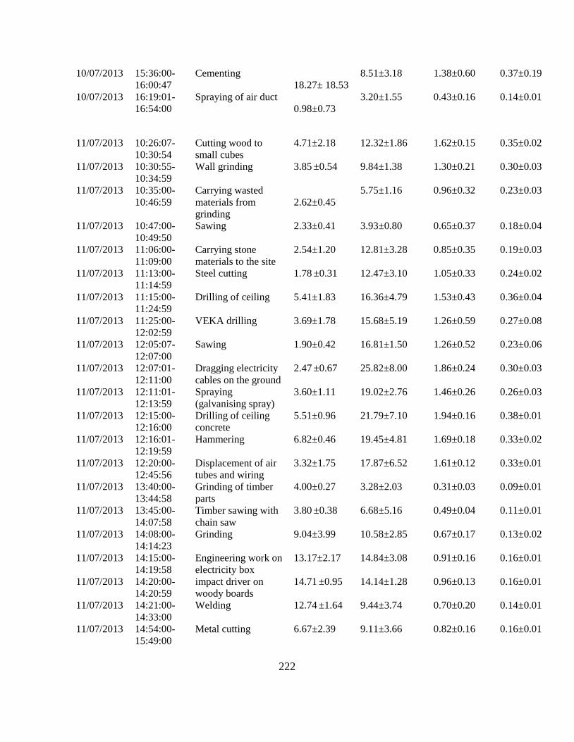
222
10/07/2013 15:36:00-
16:00:47
Cementing
18.27± 18.53
8.51±3.18 1.38±0.60 0.37±0.19
10/07/2013 16:19:01-
16:54:00
Spraying of air duct
0.98±0.73
3.20±1.55 0.43±0.16 0.14±0.01
11/07/2013 10:26:07-
10:30:54
Cutting wood to
small cubes
4.71±2.18
12.32±1.86 1.62±0.15 0.35±0.02
11/07/2013 10:30:55-
10:34:59
Wall grinding 3.85 ±0.54
9.84±1.38 1.30±0.21 0.30±0.03
11/07/2013 10:35:00-
10:46:59
Carrying wasted
materials from
grinding
2.62±0.45
5.75±1.16 0.96±0.32 0.23±0.03
11/07/2013 10:47:00-
10:49:50
Sawing 2.33±0.41
3.93±0.80 0.65±0.37 0.18±0.04
11/07/2013 11:06:00-
11:09:00
Carrying stone
materials to the site
2.54±1.20
12.81±3.28 0.85±0.35 0.19±0.03
11/07/2013 11:13:00-
11:14:59
Steel cutting 1.78 ±0.31
12.47±3.10 1.05±0.33 0.24±0.02
11/07/2013 11:15:00-
11:24:59
Drilling of ceiling 5.41±1.83
16.36±4.79 1.53±0.43 0.36±0.04
11/07/2013 11:25:00-
12:02:59
VEKA drilling 3.69±1.78
15.68±5.19 1.26±0.59 0.27±0.08
11/07/2013 12:05:07-
12:07:00
Sawing 1.90±0.42
16.81±1.50 1.26±0.52 0.23±0.06
11/07/2013 12:07:01-
12:11:00
Dragging electricity
cables on the ground
2.47 ±0.67
25.82±8.00 1.86±0.24 0.30±0.03
11/07/2013 12:11:01-
12:13:59
Spraying
(galvanising spray)
3.60±1.11
19.02±2.76 1.46±0.26 0.26±0.03
11/07/2013 12:15:00-
12:16:00
Drilling of ceiling
concrete
5.51±0.96
21.79±7.10 1.94±0.16 0.38±0.01
11/07/2013 12:16:01-
12:19:59
Hammering 6.82±0.46
19.45±4.81 1.69±0.18 0.33±0.02
11/07/2013 12:20:00-
12:45:56
Displacement of air
tubes and wiring
3.32±1.75
17.87±6.52 1.61±0.12 0.33±0.01
11/07/2013 13:40:00-
13:44:58
Grinding of timber
parts
4.00±0.27
3.28±2.03 0.31±0.03 0.09±0.01
11/07/2013 13:45:00-
14:07:58
Timber sawing with
chain saw
3.80 ±0.38
6.68±5.16 0.49±0.04 0.11±0.01
11/07/2013 14:08:00-
14:14:23
Grinding 9.04±3.99
10.58±2.85 0.67±0.17 0.13±0.02
11/07/2013 14:15:00-
14:19:58
Engineering work on
electricity box
13.17±2.17
14.84±3.08 0.91±0.16 0.16±0.01
11/07/2013 14:20:00-
14:20:59
impact driver on
woody boards
14.71 ±0.95
14.14±1.28 0.96±0.13 0.16±0.01
11/07/2013 14:21:00-
14:33:00
Welding 12.74 ±1.64
9.44±3.74 0.70±0.20 0.14±0.01
11/07/2013 14:54:00-
15:49:00
Metal cutting 6.67±2.39
9.11±3.66 0.82±0.16 0.16±0.01

223
11/07/2013 15:50:00-
16:09:30
Fiberglass cutting 2.95±0.69
9.52±3.34 0.92±0.26 0.17±0.03
11/07/2013 16:25:00-
16:29:00
Ladder movement 1.95±1.22
23.43±16.04 1.67±0.21 0.26±0.03
11/07/2013 16:29:21-
16:30:20
drilling 15.49 ±15.45
38.27±16.92 4.28±0.22 0.75±0.03
11/07/2013 16:39:00-
16:58:30
Wall drilling 3.41±1.22
14.25±4.92 1.05±0.21 0.20±0.03
11/07/2013 16:59:01-
17:01:20
grinding 4.93±3.58
6.64±0.90 0.65±0.05 0.15±0.009
11/07/2013 17:05:29-
16:06-29
Hot air torching 3.21±0.82
8.02±1.82 0.61±0.09 0.15±0.009
11/07/2013 17:07:30-
17:40:40
Preparation to finish 3.32±1.82
9.59±2.12 0.79±0.10 0.17±0.09
Table B2: Peak diameters of PND observed during different activities. It is worth noting that these
peak diameters represent the size distributions when the activities below were occurring dominantly
at the sample site and do not represent the direct emissions from an activity.
Activity name Peak
diameter 1
(nm)
Peak diameter 2
(nm)
Peak diameter 3
(nm)
Wall chasing 15.4 27.4 48.7
Cementing 15.4 27.4 48.7
Welding and hot air torching 15.4 27.4 48.7
Drilling 6.0 15.0 27.0
Cutting 15.4 27.4 56.2
Sawing 5.6 10.0 15.4
General Demolitiona 5.6 10.0 48.7
Hammering 15.4 27.4 56.2
Sanding 5.6 15.4 27.4
GF machiningb 5.6 15.4 27.4
Ground cleaning and sweeping 15.4 27.4 56.2
Spraying 15.4 20.5 48.7
Empting of waste materials 7.5 15.4 27.4
Wrenching 5.6 15.4 27.4
Ladder and staff movement 5.6 8.6 15.4
Grinding 15.4 27.4 48.7
Impact driving 5.6 10.0 27.4
Punching of timber 5.6 15.4 27.4
Preparation works to finish 15.4 27.4 56.2
Other activities (e.g. painting, oiling,
carrying metal bars to the site and moving
demolished debris)
15.4 27.4 48.7
aBreaking of materials such as concrete, brick and ceramic; bStraightening of metal tubing.

224
Table B3: Averages PNCs and PMCs for each activity, during the seven days of refurbishment
activities.
Activity name Average PNCs
±stdev
(×104 # cm-3)
PM10
±stdev
(×102 µg m-3)
PM2.5
±stdev
(×102 µg m-3)
PM1
±stdev
(×102 µg m-3)
Wall chasing 26.30±25.53 15.21±3.53 1.36±0.25 0.22±0.01
Cementing 12.23±8.44 7.66±1.20 1.05±0.47 0.25±0.17
Welding and hot air
torching
7.25±6.03 8.51±7.31 0.67±0.44 0.14±0.05
Drilling 5.22±4.44 12.74±10.17 1.09±0.94 0.21.±0.16
Cutting 2.96±1.46 8.34±4.96 0.77±0.47 0.16±0.09
Sawing 2.59±3.08 10.94±6.79 0.86±0.35 0.16±0.04
General demolitiona 9.33±7.97 20.01.±19.58 1.52±1.51 0.18±0.15
Hammering 4.27±3.09 7.50±6.90 0.63±0.61 0.13±0.11
Sanding 5.30±3.29 5.23±1.04 0.37±0.09 0.07±0.009
GF machiningb 2.99±0.30 15.69±16.63 0.99±0.98 0.13±0.09
Ground cleaning and
sweeping
1.92±0.62 11.02±7.49 0.93±0.56 0.13±0.04
Spraying 1.54±1.39 6.46±8.42 0.58±0.58 0.15±0.07
Empting of waste materials 1.75±1.12 10.25±7.29 0.70±0.35 0.13±0.0005
Wrenching 8.55±9.46 6.73±6.40 0.48±0.25 0.11±0.005
Ladder and staff movement 2.67±1.35 11.75±8.77 1.00±0.59 0.21±0.10
Grinding 4.67±2.73 7.09±3.09 0.72±0.35 0.15±0.08
Impact driving 12.33±3.36 14.33±0.26 1.03±0.09 0.20±0.04
Punching of timber 2.14±1.10 5.16±1.25 0.37±0.05 0.07±0.004
Preparation works to finish 4.02±0.99 7.23±3.33 0.57±0.32 0.12±0.07
Other activities (e.g.
painting, oiling, carrying
metal bars to the site and
moving demolished debris)
4.32±4.87 13.92±11.94 1.04±0.92 0.13±0.08
aBreaking of materials such as concrete, brick and ceramic; b Straightening of metal tubing.
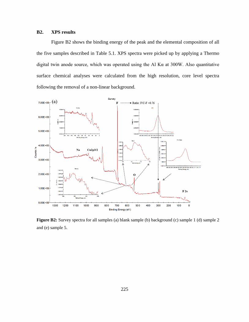
225
B2. XPS results
Figure B2 shows the binding energy of the peak and the elemental composition of all
the five samples described in Table 5.1. XPS spectra were picked up by applying a Thermo
digital twin anode source, which was operated using the Al Kα at 300W. Also quantitative
surface chemical analyses were calculated from the high resolution, core level spectra
following the removal of a non-linear background.
Figure B2: Survey spectra for all samples (a) blank sample (b) background (c) sample 1 (d) sample 2
and (e) sample 5.
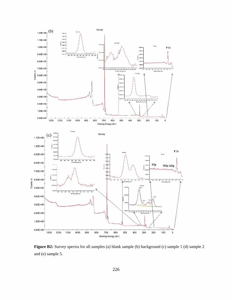
226
Figure B2: Survey spectra for all samples (a) blank sample (b) background (c) sample 1 (d) sample 2
and (e) sample 5.
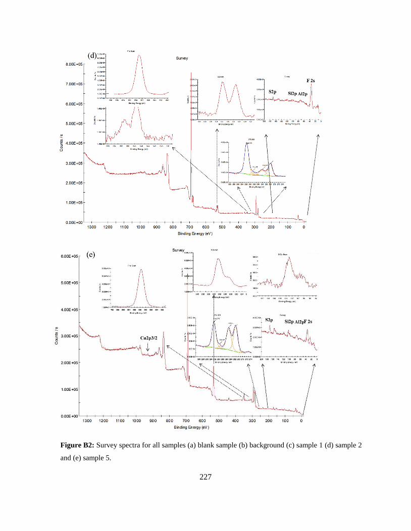
227
Figure B2: Survey spectra for all samples (a) blank sample (b) background (c) sample 1 (d) sample 2
and (e) sample 5.
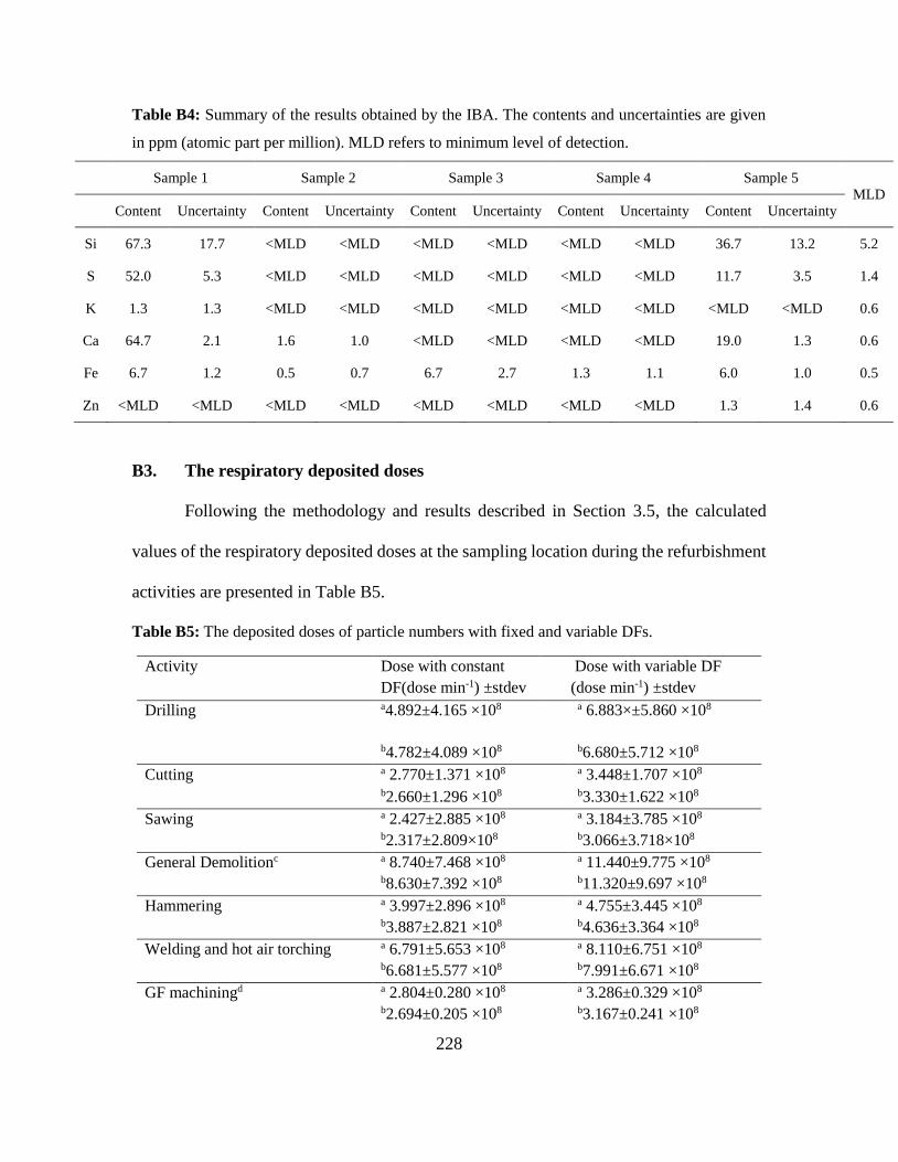
228
Table B4: Summary of the results obtained by the IBA. The contents and uncertainties are given
in ppm (atomic part per million). MLD refers to minimum level of detection.
Sample 1 Sample 2 Sample 3 Sample 4 Sample 5 MLD
Content Uncertainty Content Uncertainty Content Uncertainty Content Uncertainty Content Uncertainty
Si 67.3 17.7 <MLD <MLD <MLD <MLD <MLD <MLD 36.7 13.2 5.2
S 52.0 5.3 <MLD <MLD <MLD <MLD <MLD <MLD 11.7 3.5 1.4
K 1.3 1.3 <MLD <MLD <MLD <MLD <MLD <MLD <MLD <MLD 0.6
Ca 64.7 2.1 1.6 1.0 <MLD <MLD <MLD <MLD 19.0 1.3 0.6
Fe 6.7 1.2 0.5 0.7 6.7 2.7 1.3 1.1 6.0 1.0 0.5
Zn <MLD <MLD <MLD <MLD <MLD <MLD <MLD <MLD 1.3 1.4 0.6
B3. The respiratory deposited doses
Following the methodology and results described in Section 3.5, the calculated
values of the respiratory deposited doses at the sampling location during the refurbishment
activities are presented in Table B5.
Table B5: The deposited doses of particle numbers with fixed and variable DFs.
Activity Dose with constant
DF(dose min-1) ±stdev
Dose with variable DF
(dose min-1) ±stdev
Drilling
a4.892±4.165 ×10⁸
b4.782±4.089 ×10⁸
a 6.883×±5.860 ×10⁸
b6.680±5.712 ×10⁸
Cutting a 2.770±1.371 ×10⁸ a 3.448±1.707 ×10⁸
b2.660±1.296 ×10⁸ b3.330±1.622 ×10⁸
Sawing a 2.427±2.885 ×10⁸ a 3.184±3.785 ×10⁸
b2.317±2.809×10⁸ b3.066±3.718×10⁸
General Demolitionc a 8.740±7.468 ×10⁸ a 11.440±9.775 ×10⁸
b8.630±7.392 ×10⁸ b11.320±9.697 ×10⁸
Hammering a 3.997±2.896 ×10⁸ a 4.755±3.445 ×10⁸
b3.887±2.821 ×10⁸ b4.636±3.364 ×10⁸
Welding and hot air torching a 6.791±5.653 ×10⁸ a 8.110±6.751 ×10⁸
b6.681±5.577 ×10⁸ b7.991±6.671 ×10⁸
GF machiningd a 2.804±0.280 ×10⁸ a 3.286±0.329 ×10⁸
b2.694±0.205 ×10⁸ b3.167±0.241 ×10⁸

229
Ground cleaning and sweeping a 1.801±0.586 ×10⁸ a 2.250±0.733 ×10⁸
b1.691±0.511 ×10⁸ b2.132±0.644 ×10⁸
Wall chasing a 24.621±23.902 ×10⁸ a 30.023±29.147 ×10⁸
b24.511±23.827 ×10⁸ b29.904±29.068 ×10⁸
Spraying a 1.446±1.308 ×10⁸ a 1.763±1.595 ×10⁸
b1.366±1.233 ×10⁸ b1.644±1.517 ×10⁸
Empting of waste materials a 1.640± 1.052 ×10⁸ a 2.101±1.348 ×10⁸
b1.530±0.976 ×10⁸ b1.983±1.266 ×10⁸
Wrenching a 8.003±8.858 ×10⁸ a 10.035±11.107 ×10⁸
b7.893±8.782 ×10⁸ b9.916±11.03 ×10⁸
Ladder and staff movement a 2.501±1.269 ×10⁸ a 3.389±1.719 ×10⁸
b2.391±1.194 ×10⁸ b3.270±1.632 ×10⁸
Cementing a 11.450±7.903 ×10⁸ a 13.792±9.520 ×10⁸
b11.340±7.828 ×10⁸ b13.674±9.439 ×10⁸
Grinding a 4.379±2.558 ×10⁸ a 5.252±3.069 ×10⁸
b4.269±2.483 ×10⁸ b5.134±2.986 ×10⁸
Sanding a 4.966±3.082 ×10⁸ a 4.890±3.035 ×10⁸
b4.586±3.007 ×10⁸ b4.772±2.955 ×10⁸
Punching of timber a 1.522±0.692 ×10⁸ a 2.103±0.956 ×10⁸
b1.412±0.616 ×10⁸ b1.985±0.866 ×10⁸
Preparation to finish a 3.769±0.932 ×10⁸ a 4.333±1.072 ×10⁸
b3.659±0.857 ×10⁸ b4.215 ±0.987 ×10⁸
Impact driving a 11.546±3.146 ×10⁸ a 14.770±4.024 ×10⁸
b11.436±3.070 ×10⁸ b14.652±3.935 ×10⁸ eOther activities a 4.050±4.567 ×10⁸ a 4.962±5.596 ×10⁸
b3.940±4.492 ×10⁸ b4.843±5.521 ×10⁸
Non-activity a 2.861±2.179 ×10⁸ a 3.573±2.721 ×10⁸
b2.759±2.104 ×10⁸ b3.455±2.641 ×10⁸
Background a 0.118±0.002 ×10⁸ a 0.109± 0.081 ×10⁸
b0±0.000 ×10⁸ b0± 0.000× 10⁸
aTotal deposited doses (including background); bNet deposited doses (after subtracting background from total); cBreaking of materials such as concrete, brick and ceramic; dStraightening of metal tubing; ePainting, oiling, carrying metal bars to the site and moving demolished debris.

230
Appendix C
C1. Particle mass concentrations
Figures C1 and C2 show the average PM10 and PM2.5 during the activity and non-
activity periods at the CS1, CS2 and CS3, respectively (Tables C1- C4).
C2. Variation of PM10 and PM2.5 during different years
In order to understand the variability in concentrations during individual years, we
plotted Figures C3 and C4 that present the annual mean PM10 concentrations obtained from
monitoring stations (MS1 to MS9) around the CS1. These annual mean concentrations of
PM10 and PM2.5 ranged from 10 to 80 μg m−3 (Figure C3) and 5 to 55 μg m−3 (Figure C4),
respectively. Figure C3 also shows PM10 values at 6 monitoring stations during 5 years
(2009-2013) of measurements around the CS2. The annual mean PM10 concentrations
obtained from monitoring stations (MS10 to MS15) around the CS2 ranged from 5 to 62 μg
m−3. Moreover Figure C3 shows PM10 values during 2011 and 2012 at MS16 and MS17
around the CS3. The annual mean PM10 concentrations were found to be in the 6 to 90 μg
m−3 range with the mean of 28.90 and 32.99 μg m−3 at MS16 and MS17, respectively.
Moreover, Figure C5 presents a total number of exceedences over the EU limit value at the
individual monitoring stations.

231
Figure C1: The average concentrations of PM10 (17 monitoring stations) during the working and
non-working periods at the (a) CS1, (b) CS2, and (c) CS3.
0
20
40
60
80
100
Act
ivit
y
No
n-a
ctiv
ity
Act
ivit
y
No
n-a
ctiv
ity
Act
ivit
y
No
n-a
ctiv
ity
Act
ivit
y
No
n-a
ctiv
ity
Act
ivit
y
No
n-a
ctiv
ity
2009 2010 2011 2012 2013
MS10 MS11 MS12 MS13 MS14 MS15
0
20
40
60
80
100
Act
ivit
y
No
n-a
ctiv
ity
Act
ivit
y
No
n-a
ctiv
ity
Act
ivit
y
No
n-a
ctiv
ity
Act
ivit
y
No
n-a
ctiv
ity
Act
ivit
y
No
n-a
ctiv
ity
2002 2003 2004 2005 2006
MS1 MS2 MS3 MS4 MS5 MS6 MS7 MS8 MS9P
M1
0(µ
g m
–3)
0
20
40
60
80
100
Activity Non-activity Activity Non-activity
2011 2012
MS16 MS17
(b)
(a)
(c)

232
Figure C2: The average concentrations of PM2.5 (monitoring stations) during the working and non-
working periods at CS1.
PM
2.5
(µg m
–3)
0
10
20
30
40
50
Act
ivit
y
Non-a
ctiv
ity
Act
ivit
y
Non-a
ctiv
ity
Act
ivit
y
Non-a
ctiv
ity
Act
ivit
y
Non-a
ctiv
ity
Act
ivit
y
Non-a
ctiv
ity
2002 2003 2004 2005 2006
MS1 MS2 MS3 MS4 MS5 MS6 MS7 MS8 MS9

233
Figure C3: The Box and whiskers plots showing mean, upper, middle, and lower lines of “boxes”
indicated seventy-fifth, fiftieth, and twenty-fifth percentiles of PM10 values during the activity and
non-activity periods at the monitoring stations at CS1 (red colour), CS2 (green colour), and CS3
(violet colour).
0.0
0.2
0.4
0.6
0.8
S10 S11 S12 S13 S14 S15
0.0
0.2
0.4
0.6
0.8
S10 S11 S12 S13 S14 S15
0
0.2
0.4
0.6
0.8
MS 1 MS 2 MS 3 MS 4 MS 5 MS 6 MS 7 MS 8 MS 9
PM
10
(µg m
-3)
10
2
0.0
0.2
0.4
0.6
0.8
S1 S2 S3 S4 S5 S6 S7 S8 S9
2002
0.0
0.2
0.4
0.6
0.8
S1 S2 S3 S4 S5 S6 S7 S8 S9
2004
0.0
0.2
0.4
0.6
0.8
MS 1 MS 2 MS 3 MS 4 MS 5 MS 6 MS 7 MS 8 MS 9
2005
2006
MS1
0.0
0.2
0.4
0.6
0.8
MS 10 MS 11 MS 12 MS 13 MS 14 MS 15
0.0
0.2
0.4
0.6
0.8
S10 S11 S12 S13 S14 S15
Monitoring stations
2009
2010 2011
0.0
0.2
0.4
0.6
0.8
MS 10 MS 11 MS 12 MS 13 MS 14 MS 15
2012 2013
0.0
0.2
0.4
0.6
0.8
MS 16 MS 17
0.0
0.2
0.4
0.6
0.8
MS 16 MS 17
20122011
MS2 MS3MS4MS5 MS6MS7 MS8 MS9 MS1MS2 MS3 MS4 MS5MS6MS7MS8MS9
MS1 MS2 MS3MS4MS5 MS6 MS7MS8MS9MS1 MS2 MS3MS4MS5 MS6MS7 MS8 MS9
MS2 MS3MS4MS5 MS6MS7 MS8 MS9MS1 MS10 MS11 MS12 MS13 MS14 MS15
MS10 MS11 MS12 MS13 MS14 MS15 MS10 MS11 MS12 MS13 MS14 MS15
MS10 MS11 MS12 MS13 MS14 MS15 MS10 MS11 MS12 MS13 MS14 MS15
MS16 MS17 MS16 MS17
0.8
0.6
0.4
0.2
0.0
0.8
0.6
0.4
0.2
0.0
0.8
0.6
0.4
0.2
0.0
0.8
0.6
0.4
0.2
0.0
0.8
0.6
0.4
0.2
0.0
0.8
0.6
0.4
0.2
0.0
0.0
0.2
0.4
0.6
0.8
s 1 s 2 s 3 s 4 s 5 s 6 s 7 s 8 s 9
2003

234
Figure C4: The Box and whiskers plots showing mean, upper, middle, and lower lines of “boxes”
indicated seventy-fifth, fiftieth, and twenty-fifth percentiles of PM2.5 values during the activity and
non-activity periods at the monitoring stations at CS1.
0.0
0.2
0.3
0.5
0.6
MS 1 MS 2 MS 3 MS 4 MS 5 MS 6 MS 7 MS 8 MS 9
0.0
0.2
0.3
0.5
0.6
MS 1 MS 2 MS 3 MS 4 MS 5 MS 6 MS 7 MS 8 MS 9
0.0
0.2
0.3
0.5
0.6
s 1 s 2 s 3 s 4 s 5 s 6 s 7 s 8 s 9
PM
2.5
(µg m
-3)
10
2
Monitoring stations
2003
0.0
0.2
0.3
0.5
0.6
S1 S2 S3 S4 S5 S6 S7 S8 S9
2004
0.0
0.2
0.3
0.5
0.6
S1 S2 S3 S4 S5 S6 S7 S8 S9
2002
2005
2006
MS1 MS2 MS3 MS4 MS5 MS6 MS7MS9MS8
MS1 MS2 MS3 MS4 MS5 MS6 MS7MS9MS8
0.6
0.5
0.3
0.2
0.0
0.6
0.5
0.3
0.2
0.0
0.6
0.5
0.3
0.2
0.0

235
Figure C5: Total number of exceedences over the EU limit value at the individual monitoring
stations.
0 10 20 30 40 50 60
S16
S17 20112010
0 10 20 30 40 50 60
S10
S11
S12
S13
S14
S152013
2012
2011
2010
2009
0 10 20 30 40 50 60
S1
S2
S3
S4
S5
S6
S7
S8
S9 2006
2005
2004
2003
2002
Number of exceedence days
Mo
nit
ori
ng s
tati
on
s
MS1MS1
MS1
MS1
MS1
MS1
MS1
MS1
MS1
MS1
MS1
MS1
MS1
MS1
MS1
MS2
MS3
MS4
MS5
MS6
MS7
MS8
MS9
MS10
MS11
MS12
MS13
MS14
MS15
MS16
MS17
EU limit value:
(not to be exceeded 50 µg m-3 more than 35 times a year)

236
Table C1: The concentrations of PM10 during the working and non-working periods at the CS2;
STD refers to standard deviation and “–” to the unavailability of data.
Monitoring
stations
Year PM10 MS10 MS11 MS12 MS13 MS14 MS15
2009 Working 29.006±16.77 20.30±11.82 20.05±11.60 15.69±8.01 _ 16.57±9.67
Non-working 20.72±14.30 16.26±10.35 18.64±11.58 13.81±7.79 _ 14.52±8.77
2010 Working 25.31±15.51 18.97±12.89 _ 16.84±12.89 _ 16.05±11.90
Non-working 22.06±18.27 15.57±9.57 _ 14.64±14.97 _ 13.57±8.71
2011 Working 27.74±18.23 20.35±12.43 _ 21.59±12.89 _ 20.91±12.81
Non-working 22.46±18.46 17.22±12.95 _ 19.22±10.88 _ 19.20±13.68
2012 Working 24.92±17.53 19.88±14.22 _ 17.22±10.27 _ 18.98±14.93
Non-working 19.48±14.82 17.48±13.19 _ 15.62±9.28 _ 17.16±16.05
2013 Working 20.71±12.82 17.60±10.39 _ 21.75±12.36 19.36±12.76 20.77±16.22
Non-working 18.72±12.90 13.68±8.40 _ 18.30±10.04 15.50±10.21 17.54±10.97
Overall
Working 25.54±3.18 19.42±1.15
20.056±0.00
18.36±2.84 19.36±0.00
18.66±2.27
Overall
Non-working 20.69±1.60 16.04±0.33
18.64±0.00 16.32±2.33
15.50±0.00
16.40±2.30
Table C2: The concentrations of PM10 during the working and non-working periods at the CS3;
STD refers to standard deviation.
Monitoring stations
Year PM10 MS16 MS17
2011 Working 29.006±16.77 20.30±11.82
Non-working 20.72±14.30 16.26±10.35
2012 Working 25.31±15.51 18.97±12.89
Non-working 22.06±18.27 15.57±9.57
Overall
Working 46.62±8.82 49.84±5.66
Overall Non-working 19.30±3.62 24.16±1.11

237
Table C3: The concentrations of PM10 during the working and non-working periods at the CS1; STD refers to
standard deviation, W to working, N-w to non-working and “–” to the unavailability of data.
Monitoring stations
Year PM10 MS1 MS2 MS3 MS4 MS5 MS6 M S7 M S8 M S9
2002 W _ 23.34±12.60 20.64±12.19 36.29±27.47 32.74±26.12 26.71±19.46 20.19±11.04 20.45±10.89 27.64±16.69
N-w _ 20.54±11.95 17.65±10.20 22.89±17.30 22.37±15.79 20.51±11.78 18.56±10.11 18.38±9.53 21.08±12.14
2003 W _ 25.98±15.82 22.23±12.60 46.56±39.31 30.04±21.49 36.67±29.53 22.67±13.91 25.81±16.99 24.46±15.09
N-w _ 23.16±15.68 20.28±13.37 26.90±24.96 23.61±15.80 25.95±26.33 21.65±14.15 21.94±14.09 19.83±12.33
2004 W 20.84±12.57 22.66±12.25 18.22±9.59 34.62±27.47 23.46±13.20 30.56±37.97 19.96±12.64 21.74±12.69 29.56±19.90
N-w 18.78±10.60 19.85±11.72 16.42±9.45 23.27±19.70 20.15±13.08 19.73±13.13 17.48±10.02 19.38±10.96 22.25±14.26
2005 W 20.42±11.17 25.34±12.22 18.07±12.42 31.54±26.51 24.58±13.74 27.28±20.65 19.94±10.55 20.54±10.41 _
N-w 18.78±10.15 22.51±12.05 16.76±9.47 21.88±16.62 21.89±14.61 20.62±18.16 18.37±10.32 18.78±10.06 _
2006 W 21.54±11.35 25.27±12.37 19.49±9.76 28.32±20.52 27.03±25.51 26.07±20.45 21.33±10.65 22.78±12.87 _
N-w 19.37±11.06 23.76±34.76 18.15±9.95 21.44±15.53 21.99±16.22 19.85±10.67 20.01±11.02 19.65±10.68 _
Overall W 20.93±0.56 24.52±1.43
19.73±1.74 35.47±6.90
27.56±3.83
29.46±4.38
20.82±1.18
22.26±2.43
27.22±2.57
Overall N-w 18.98±0.34 21.92±1.69
17.85±1.52 23.27±2.15
22.00±1.23
21.33±2.61
19.21±1.63
19.63±1.38 21.06±1.21
Table C4: The concentrations of PM2.5 during the working and non-working periods at the CS1; STD refers to
standard deviation, W to working, N-w to non-working and “–” to the unavailability of data.
Monitoring stations
Year PM2.5 MS1 MS2 MS3 MS4 MS5 MS6 MS7 MS8 MS9
2002 W _ _ _ 18.60±20.81 13.22±8.23 12.72±7.87 12.55±8.29 12.30±7.39 13.27±8.26
N-w _ _ _ 16.04±15.15 12.89±7.95 12.30±8.24 11.62±8.06 11.42±7.08 12.09±7.53
2003 W _ _ _ 17.28±17.77 15.16±10.48 15.09±10.47 14.95±10.91 16.06±10.76 20.27±10.66
N-w _ _ _ 13.84±9.50 14.00±10.19 12.90±9.38 13.57±9.94 15.12±10.66 14.56±9.71
2004 W _ _ _ 17.57±19.70 13.05±7.87 12.51±7.76 12.26±7.64 12.81±7.95 20.27±14.65
N-w _ _ _ 16.59±17.13 12.16±6.95 12.14±8.09 10.93±6.63 11.58±7.07 18.55±11.92
2005 W _ _ _ 16.21±18.96 13.55±8.80 12.98±8.27 12.49±8.08 12.75±7.92 _
N-w _ _ _ 14.62±13.63 12.44±7.66 12.88±8.19 11.38±7.09 11.40±7.05 _
2006 W _ _ _ 14.71±12.16 13.67±8.84 13.53±8.35 12.80±8.59 13.33±7.60 _
N-w _ _ _ 14.50±13.82 12.47±7.34 12.73±7.65 11.57±7.13 12.55±7.21 _
Overall
W
_ _ _ 16.88±1.47 13.73±0.83 13.37±1.03 13.01±1.10 13.45±1.50 17.94±2.90
Overall
N-w
_ _ _ 15.12±1.14
12.79±0.72
12.59±0.347
11.81±1.01
12.41±1.58
15.06±3.26

238
Appendix D
D1. Calibration of PM mass
Tables D1 show the description of GRIM 1.107 E calibration by the manufacturer and also
the values measured during the building demolition activity.
Table D1: Description of GRIMM 1.107 E calibration by the manufacturer.
Measurement values at calibration tower (sample volume: 0.018 m3/sample time : 15 min)
Mean value Reference unit
(µg m–3)
Calibrated unit
(µg m–3)
Deviation (%)
PM10 305.5 308.3 0.9
PM2.5 119.3 118.0 1.1
PM1 42.3 41.9 0.9
Measurement values at ambient air (sample volume: 0.9 m3 and sample time : 823 min)
Mean value Reference unit
(µg m–3)
Calibrated unit
(µg m–3)
Deviation (%)
PM10 4.7 4.5 4.3
PM2.5 4.1 3.9 4.9
PM1 3.5 3.3 5.7
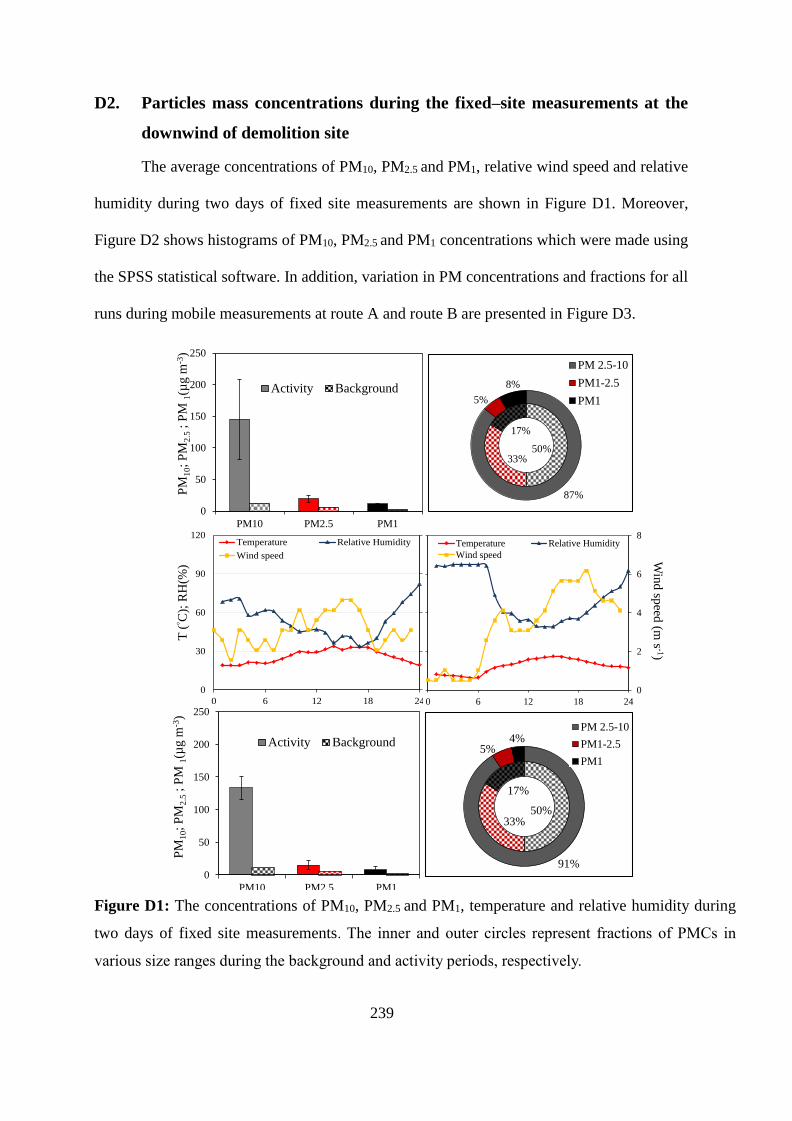
239
D2. Particles mass concentrations during the fixed–site measurements at the
downwind of demolition site
The average concentrations of PM10, PM2.5 and PM1, relative wind speed and relative
humidity during two days of fixed site measurements are shown in Figure D1. Moreover,
Figure D2 shows histograms of PM10, PM2.5 and PM1 concentrations which were made using
the SPSS statistical software. In addition, variation in PM concentrations and fractions for all
runs during mobile measurements at route A and route B are presented in Figure D3.
Figure D1: The concentrations of PM10, PM2.5 and PM1, temperature and relative humidity during
two days of fixed site measurements. The inner and outer circles represent fractions of PMCs in
various size ranges during the background and activity periods, respectively.
0
2
4
6
8
0
30
60
90
120
0 6 12 18 24
Temperature Relative Humidity
Wind speed
50%33%
17%
87%
5%
8%
0
50
100
150
200
250
PM10 PM2.5 PM1
0
2
4
6
8
0
30
60
90
120
0 6 12 18 24
Temperature Relative Humidity
Wind speed
PM
10;
PM
2.5
; P
M 1
(µg m
-3)
T ( C
); R
H(%
)
Win
d sp
eed (m
s-1)
PM
10;
PM
2.5
; P
M 1
(µg m
-3)
PM 2.5-10
PM1-2.5
PM1
50%33%
17%
91%
5%4%
PM 2.5-10
PM1-2.5
PM1
0
50
100
150
200
250
PM10 PM2.5 PM1
0
20
40
60
80
100
120
140
PM10 PM2.5 PM1
Activity Background
0
20
40
60
80
100
120
140
PM10 PM2.5 PM1
Activity Background

240
Figure D2. The concentrations of PM10, PM2.5 and PM1 related cumulative frequency during the all
days of fixed site measurements.
24-hour mean WHO guideline
value (25 µg m-3)
Fre
quen
cy (
num
ber
of
occ
urr
ence
s)
PM10 (µg m-3)
PM2.5 (µg m-3)
PM1 (µg m-3)
Concentrations (µg m-3)
Cum
ula
tive
per
cent
(%)
24-hour mean EU limit value
(50 µg m-3)
0
20
40
60
80
100
1
12
22
33
45
61
87
253
About 11 % exceeded
the WHO value
0
20
40
60
80
100
1
42
84
13
6
21
4
349
69
0
10
70
About 42 % exceeded
the EU limit
Cum
ula
tive
per
centa
ge
(%)
Concentrations (µg m-3)
Cum
ula
tive
per
cent
(%)
Concentrations (µg m-3)
0
20
40
60
80
100
1 5 8
11
15
18
23
75
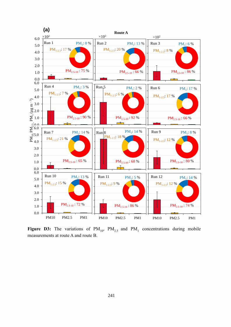
241
Figure D3: The variations of PM10, PM
2.5 and PM
1 concentrations during mobile
measurements at route A and route B.
0.0
1.0
2.0
3.0
4.0
5.0
6.0
PM10 PM2.5 PM1
0.0
1.0
2.0
3.0
4.0
5.0
6.0
PM10 PM2.5 PM1
0.0
1.0
2.0
3.0
4.0
5.0
6.0
PM10 PM2.5 PM1
0.0
1.0
2.0
3.0
4.0
5.0
6.0
PM10 PM2.5 PM1
0
1
2
3
4
5
6
PM10 PM2.5 PM1
0
1
2
3
4
5
6
PM10 PM2.5 PM1
0
1
2
3
4
5
6
PM10 PM2.5 PM10
1
2
3
4
5
6
PM10 PM2.5 PM1
0
1
2
3
4
5
6
PM10 PM2.5 PM1
0
1
2
3
4
5
6
PM10 PM2.5 PM1
PM
10
, P
M2
.5 ,
PM
1(µ
g m
–3)
Run 1 Run 2 Run 3
Run 5 Run 6
Route A
0
1
2
3
4
5
6
PM10 PM2.5 PM1
0
1
2
3
4
5
6
PM10 PM2.5 PM1
Run 7 Run 8 Run 9
Run 10 Run 11 Run 12
Run 4
(a)
102 102 102
PM1: 8 %
PM2.5-10 : 75 %
PM1: 2 %
PM2.5-10 : 92 %
PM1: 8 %
PM1-2.5: 12 %
PM2.5-10 : 80 %
PM1-2.5: 17 % PM1-2.5: 20 %
PM1: 13 %
PM2.5-10 : 66 %
PM2.5-10 : 90 %
PM2.5-10 : 86 %
PM1-2.5: 8 %
PM1: 6 %
PM1-2.5: 7 %
PM1: 3 %
PM1-2.5: 6 %PM1-2.5: 17 %
PM2.5-10 : 66 %
PM1: 17 %
PM1: 14 %
PM1-2.5: 21 %
PM2.5-10 : 65 %
PM1-2.5: 18 %
PM1: 14 %
PM2.5-10 : 68 %
PM1: 13 %
PM1-2.5: 15 %
PM2.5-10 : 72 %
PM1-2.5: 9 %
PM2.5-10 : 86 %
PM1: 5 %
PM1-2.5: 12 %
PM1: 14 %
PM2.5-10 : 74 %
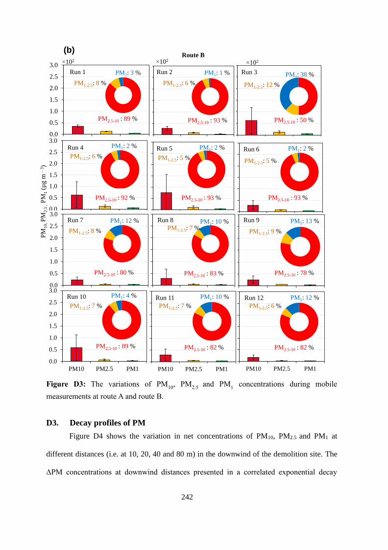
242
Figure D3: The variations of PM10, PM
2.5 and PM
1 concentrations during mobile
measurements at route A and route B.
D3. Decay profiles of PM
Figure D4 shows the variation in net concentrations of PM10, PM2.5 and PM1 at
different distances (i.e. at 10, 20, 40 and 80 m) in the downwind of the demolition site. The
ΔPM concentrations at downwind distances presented in a correlated exponential decay
0.0
0.5
1.0
1.5
2.0
2.5
3.0
PM10 PM2.5 PM1
0.0
0.5
1.0
1.5
2.0
2.5
3.0
PM10 PM2.5 PM1
0.0
0.5
1.0
1.5
2.0
2.5
3.0
PM10 PM2.5 PM1
0.0
0.5
1.0
1.5
2.0
2.5
3.0
PM10 PM2.5 PM10.0
0.5
1.0
1.5
2.0
2.5
3.0
PM10 PM2.5 PM1
0.0
0.5
1.0
1.5
2.0
2.5
3.0
PM10 PM2.5 PM1
0.0
0.5
1.0
1.5
2.0
2.5
3.0
PM10 PM2.5 PM1
0.0
0.5
1.0
1.5
2.0
2.5
3.0
PM10 PM2.5 PM1
0.0
0.5
1.0
1.5
2.0
2.5
3.0
PM10 PM2.5 PM1
0.0
0.5
1.0
1.5
2.0
2.5
3.0
PM10 PM2.5 PM1
0.0
0.5
1.0
1.5
2.0
2.5
3.0
PM10 PM2.5 PM1
0.0
0.5
1.0
1.5
2.0
2.5
3.0
PM10 PM2.5 PM1
PM
10
, P
M2
.5 ,
PM
1(µ
g m
–3)
Run 1 Run 2 Run 3
Run 5 Run 6
Route B
Run 7 Run 8 Run 9
Run 10 Run 11 Run 12
Run 4
(b)
102 102 102
PM1-2.5: 8 %
PM1: 12 %
PM2.5-10 : 80 %
PM1: 10 %PM1-2.5: 7 %
PM2.5-10 : 83 % PM2.5-10 : 78 %
PM1-2.5: 9 %
PM1: 13 %
PM1: 4 %
PM1-2.5: 7 %
PM2.5-10 : 89 %
PM1: 10 %
PM1-2.5: 7 %
PM2.5-10 : 82 %
PM1-2.5: 6 %
PM1: 12 %
PM2.5-10 : 82 %
PM1: 3 %
PM1-2.5: 6 %
PM1: 1 %
PM2.5-10 : 93 %
PM1: 38 %
PM1-2.5: 12 %
PM2.5-10 : 50 %
PM1: 2 %
PM1-2.5: 6 %
PM2.5-10 : 92 %
PM1-2.5: 5 %
PM1: 2 %
PM2.5-10 : 93 % PM2.5-10 : 93 %
PM1-2.5: 5 %
PM1: 2 %
PM1-2.5: 8 %
PM2.5-10 : 89 %

243
profiles form with R2 values as 0.85 (ΔPM10), 0.89 (ΔPM2.5) and 0.68 (ΔPM1). Moreover,
concentrations of PM10 and PM2.5 against distances and their comparison with EU and WHO
limit values are shown in Figure D5.
Figure D4. (a) ΔPM
10, (b) ΔPM
2.5 and (c) ΔPM
1 concentration decay at demolition site during days
of measurements (average of day 6 and day 7) versus distance in the downwind direction of
y = 7.30e-0.007x (R² = 0.68)
0
10
20
30
40
50
0 20 40 60 80 100
y = 23.18e-0.022x (R² = 0.89)
0
20
40
60
80
100
0 20 40 60 80 100
y = 61.53e-0.008x (R² = 0.85)
0
20
40
60
80
100
0 20 40 60 80 100
ΔP
M1
0 (µ
g m
-3)
(b)
(c)
(a)
y = -12.02ln(x) + 85.67 (R² = 0.85)
y = -2.45ln(x) + 19.33 (R² = 0.93)
y = -2.11ln(x) + 14.20 (R² = 0.84)
0
20
40
60
80
100
0 20 40 60 80 100
PM10
PM2.5
PM1
Log. (PM10)
Log. (PM2.5)
Log. (PM1)
y = -12.02ln(x) + 85.67 (R² = 0.85)
y = -2.45ln(x) + 19.33 (R² = 0.93)
y = -2.11ln(x) + 14.20 (R² = 0.84)
0
20
40
60
80
100
0 20 40 60 80 100
PM10
PM2.5
PM1
Log. (PM10)
Log. (PM2.5)
Log. (PM1)
y = -12.02ln(x) + 85.67 (R² = 0.85)
y = -2.45ln(x) + 19.33 (R² = 0.93)
y = -2.11ln(x) + 14.20 (R² = 0.84)
0
20
40
60
80
100
0 20 40 60 80 100
PM10
PM2.5
PM1
Log. (PM10)
Log. (PM2.5)
Log. (PM1)
y = -15.13ln(x) + 123.52 (R² = 0.94)
y = -14.57ln(x) + 74.02 (R² = 0.92)
y = -1.44ln(x) + 13.06 (R² = 0.83)
0
20
40
60
80
100
0 20 40 60 80 100
PM10
PM2.5
PM1
Log. (PM10)
Log. (PM2.5)
Log. (PM1)
ΔP
M2
.5 (µ
g m
-3)
ΔP
M1
(µg m
-3)
Distance (m)
y = 61.53e-0.008x (R² = 0.85)
0
20
40
60
80
100
0 20 40 60 80 100
PM10
Expon. ( )
y = -15.13ln(x) + 123.52 (R² = 0.94)
y = -14.57ln(x) + 74.02 (R² = 0.92)
y = -1.44ln(x) + 13.06 (R² = 0.83)
0
20
40
60
80
100
0 20 40 60 80 100
PM10
PM2.5
PM1
Log. (PM10)
Log. (PM2.5)
Log. (PM1)
y = 61.53e-0.008x (R² = 0.85)
0
20
40
60
80
100
0 20 40 60 80 100
PM10
Expon. ( )
y = -15.13ln(x) + 123.52 (R² = 0.94)
y = -14.57ln(x) + 74.02 (R² = 0.92)
y = -1.44ln(x) + 13.06 (R² = 0.83)
0
20
40
60
80
100
0 20 40 60 80 100
PM10
PM2.5
PM1
Log. (PM10)
Log. (PM2.5)
Log. (PM1)
y = 7.30e-0.007x (R² = 0.68)
0
10
20
30
40
50
0 20 40 60 80 100
PM1
PM1
PM1
Expon. ( )
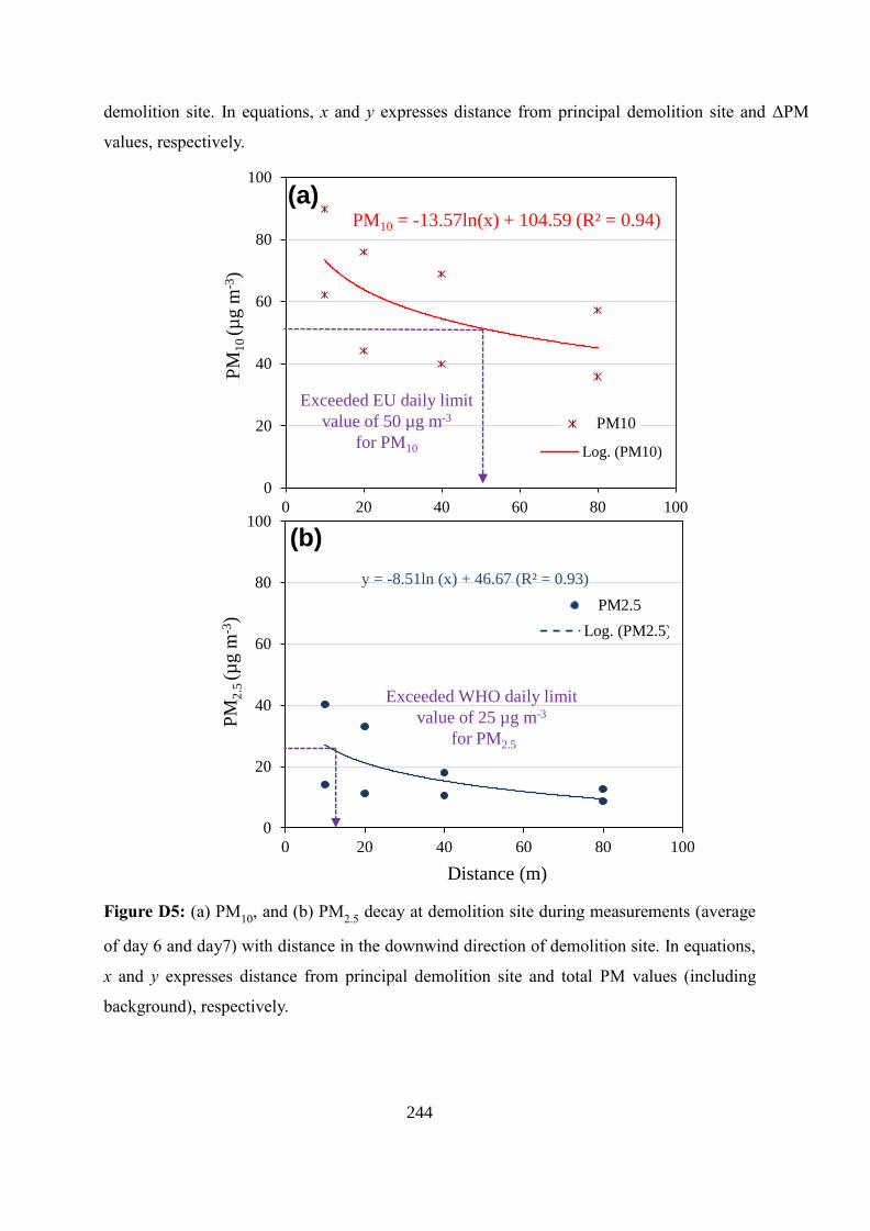
244
demolition site. In equations, x and y expresses distance from principal demolition site and ΔPM
values, respectively.
Figure D5: (a) PM10, and (b) PM
2.5 decay at demolition site during measurements (average
of day 6 and day7) with distance in the downwind direction of demolition site. In equations,
x and y expresses distance from principal demolition site and total PM values (including
background), respectively.
y = -8.51ln (x) + 46.67 (R² = 0.93)
0
20
40
60
80
100
0 20 40 60 80 100
PM10 = -13.57ln(x) + 104.59 (R² = 0.94)
0
20
40
60
80
100
0 20 40 60 80 100
PM
10
(µ
g m
-3)
(b)
(a)
y = -12.02ln(x) + 85.67 (R² = 0.85)
y = -2.45ln(x) + 19.33 (R² = 0.93)
y = -2.11ln(x) + 14.20 (R² = 0.84)
0
20
40
60
80
100
0 20 40 60 80 100
PM10
PM2.5
PM1
Log. (PM10)
Log. (PM2.5)
Log. (PM1)
y = -12.02ln(x) + 85.67 (R² = 0.85)
y = -2.45ln(x) + 19.33 (R² = 0.93)
y = -2.11ln(x) + 14.20 (R² = 0.84)
0
20
40
60
80
100
0 20 40 60 80 100
PM10
PM2.5
PM1
Log. (PM10)
Log. (PM2.5)
Log. (PM1)
y = -12.02ln(x) + 85.67 (R² = 0.85)
y = -2.45ln(x) + 19.33 (R² = 0.93)
y = -2.11ln(x) + 14.20 (R² = 0.84)
0
20
40
60
80
100
0 20 40 60 80 100
PM10
PM2.5
PM1
Log. (PM10)
Log. (PM2.5)
Log. (PM1)
y = -15.13ln(x) + 123.52 (R² = 0.94)
y = -14.57ln(x) + 74.02 (R² = 0.92)
y = -1.44ln(x) + 13.06 (R² = 0.83)
0
20
40
60
80
100
0 20 40 60 80 100
PM10
PM2.5
PM1
Log. (PM10)
Log. (PM2.5)
Log. (PM1)
PM
2.5
(µ
g m
-3)
Distance (m)
Exceeded EU daily limit
value of 50 µg m-3
for PM10
Exceeded WHO daily limit
value of 25 µg m-3
for PM2.5

245
D4. Estimation of particle mass emission factors (PMEF)
Emission factors of PM10, PM2.5 and PM1 from demolition works (applying the
modified box model) is shown in Table D2 and their summary is presented in Figure D6.
Figure D6. Particle mass concentration based PMEFs demolition activity.
Table D2. Net PM10, PM2.5 and PM1 emission factors from demolition work activity after
applying the modified box model.
PM10, PM2.5 and PM1 net emission factors (excluding background values)
ΔPM10
(µg m–3)
ΔPM2.5
(µg m–3)
ΔPM1
(µg m–3)
UX
(m s-1)
Hm
(m)
W
(m)
EFPM10
(µg m–2 s–1)
EFPM2.5
(µg m–2 s–1)
EFPM1
(µg m–2 s–1)
Day 1 123.81 60.19 15.66 0.50 8.40 15.00 34.67±17.09 16.85±3.07 4.38±0.03
Day 2 123.81 60.19 15.66 0.52 8.40 15.00 36.05±8.15 17.52±4.32 4.56±1.07
Average 123.81 60.19 15.66 0.51 8.40 15.00 35.36±12.72 17.19±3.69 4.47±0.54
D5. Energy dispersive X-ray spectroscopy technique (EDS) analysis
Figure D7 shows the EDS survey spectra and binding energy of the peak for
understanding the elemental composition of all the five samples described in Table 3.5. In
0
5
10
15
20
PM10 PM2.5 PM1
Demolition activity
Europe (EMEP-EEA)
UK (NAEI)
PM type
PM
Em
issi
on F
acto
r (µ
g m
-2kg -1
)
PM10 PM2.5 PM1
103

246
addition, Table D3 shows potential sources of captured elements on the filters in the typical
urban environment.
Figure D7. EDS survey spectra for sample 1 (reference), sample 2 (background) and samples
3-5 (demolition period).
Sample1(Reference)
Sample 2 (Background)
Sample 3
Sample 4
Sample 5
Binding Energy (keV)
Counts
/sC
ounts
/sC
ounts
/sC
ounts
/sC
ounts
/s

247
Table D3. Main potential sources of captured elements on the filters (Friedlander, 1973; Fuge
and Andrews, 1988; Kowalczyk et al., 1982; Miguel et al., 1997; Viana et al., 2008).
Elements Possible sources in urban environments Possible links with building demolition
C Tire dust; Auto exhaust; Fuel oil fly ash Could be released from exhaust of the construction
heavy vehicular in the form calcium carbonate as
filler in many construction materials
O Sea spray; Tire dust; Auto exhaust; Fuel
oil fly ash
Contributing to the elements in oxide form
F Fuel oil fly ash Could be found in building materials (steel)
Na Sea spray; Soil dust Could be found in building materials (Portland
cement)
N Sea spray; Soil dust; Auto exhaust Could be found in building materials such
incandescent and fluorescent light bulbs
S Sea spray; Auto exhaust; Fuel oil fly
ash
Could be found in building materials (Portland
cement)
Cl Sea spray; Auto exhaust Could be found in building materials (Gypsum)
Al Soil dust; Auto exhaust Could be found in building materials (Metal and
Ceramic)
Mg Sea spray; Tire dust; Fuel oil fly ash Could be found in building materials (Portland
cement)
Si Soil dust; Fuel oil fly ash Could be found in building materials (Portland
cement, bricks, asbestos)
Zn Auto exhaust; Fuel oil fly ash Could be found in building materials (metals)

248
D6. Estimation of the respiratory deposited doses (RDD)
The average RDD of coarse and fine particles during demolition works were calculated
using the approach described in Section 3.5 and were shown in Figure D8.
Figure D8. Respiratory deposition dose (RDD) rate (µg min−1) calculated using a constant
DF and the average PMCs for coarse and fine particles during each activity.
Respiratory deposition doses for coarse and fine particles (µg min-1)
Act
ivit
y t
yp
e
0 5 10 15 20 25 30 35
Heavy
Light
Heavy
Light
Heavy
Light
Heavy
Light
Heavy
Light
Heavy
Light
Heavy
Light
Heavy
Light
Heavy
Light
Heavy
Light
Heavy
Light
Heavy
Light
Heavy
Light
Heavy
Light
Heavy
Light
Heavy
LightM
ale
Mal
eF
emal
eM
ale
Fem
ale
Mal
eF
emal
eM
ale
Fem
ale
Mal
eF
emal
eM
ale
Fem
ale
Mal
eM
ale
Fem
ale
Const
ru
ctio
n
site
(fix
ed
site
)
Aro
und t
he
const
ruct
ion s
ite
(Route
A)
Aro
und t
he
const
ruct
ion s
ite
(Route
B)
At
dif
fere
nt
dis
tance
s fr
om
the
const
ruct
ion
site
(10 m
)
At
dif
fere
nt
dis
tance
s fr
om
the
const
ruct
ion
site
(10 m
)
At
dif
fere
nt
dis
tance
s fr
om
the
const
ruct
ion
site
(40 m
)
At
dif
fere
nt
dis
tance
s fr
om
the
const
ruct
ion
site
(80 m
)
Insi
de
the
exca
vat
or
cabin
Insi
de
the
conta
iner
off
ice
Fine particles
Coarse partciles

249
References
Friedlander, S.K., 1973. Chemical element balances and identification of air pollution sources.
Environmental Science & Technology 7, 235-240.
Fuge, R., Andrews, M., 1988. Fluorine in the UK environment. Environmental Geochemistry
and Health 10, 96-104.
Kowalczyk, G.S., Gordon, G.E., Rheingrover, S.W., 1982. Identification of atmospheric
particulate sources in Washington, D.C. using chemical element balances.
Environmental Science & Technology 16, 79-90.
Miguel, E.D., Llamas, J.F., Chacon, E., Berg, T., Larssen, S., Royset, O., Vadset, M., 1997.
Origin and patterns of distribution of trace elements in street dust: Unleaded petrol and
urban lead. Atmospheric Environment 31, 2733-2740.
Viana, M., Kuhlbusch, T., Querol, X., Alastuey, A., Harrison, R., Hopke, P., Winiwarter, W.,
Vallius, M., Szidat, S., Prevot, A., 2008. Source apportionment of particulate matter
in Europe: a review of methods and results. Journal of Aerosol Science 39, 827-849.