Unclassified Organisation de Coopération et de Développement Economiques Organisation for Economic Co-operation and Development __________________________________________________________________________________________ English text only ENVIRONMENT DIRECTORATE JOINT MEETING OF THE CHEMICALS COMMITTEE AND THE WORKING PARTY ON CHEMICALS, PESTICIDES AND BIOTECHNOLOGY

OECD SERIES ON EMISSION SCENARIO DOCUMENTS Number 2 Emission Scenario Document for Wood Preservatives PART 1

Unclassified

E

nglish text only

Document n’est pas disponible sur OLIS Document is not available on OLIS

Emission Scenario Document for Wood Preservatives

[Part 1]

1

TABLE OF CONTENTS

FOREWORD...................................................................................................................................................2

1. GENERAL INTRODUCTION ................................................................................................................3

1.1 Background .......................................................................................................................................3 1.2 Rationale for guidance on the environmental exposure assessment to wood preservatives .............3 1.3 Life cycle of wood preservatives ......................................................................................................4 1.4 Structure of the document .................................................................................................................5

2. MAIN TREATMENT TYPES, PRODUCT TYPES AND USES OF TREATED WOOD......................6

2.1 Main treatment types and processes..................................................................................................6 2.2 Main wood preservative product types .............................................................................................9 2.3 Main uses of treated wood ..............................................................................................................12

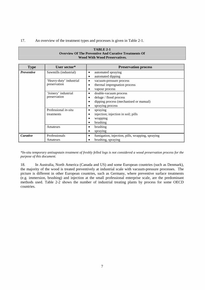
3. PRINCIPLES OF ENVIRONMENTAL RISK ASSESSMENT FOR WOOD PRESERVATIVES.......14

3.1 Stages of risk assessment ................................................................................................................14 3.2 Environmental exposure assessment...............................................................................................15 3.3 Spatial scales ...................................................................................................................................16 3.4 Time scale .......................................................................................................................................16 3.5 Focus of the document ....................................................................................................................17 3.6 Selection of emission scenarios ......................................................................................................19

3.6.1 Scenarios for the life stage of product application ....................................................................19 3.6.2 Scenarios for the life stage of wood-in-service .........................................................................19

4. EMISSION ESTIMATION FOR INDUSTRIAL PREVENTIVE PROCESSES..................................20

4.1 General considerations ....................................................................................................................20 4.1.1 Post-treatment conditioning.......................................................................................................20 4.1.2 Storage of treated wood prior to shipment ................................................................................21 4.1.3 Environmental compartments exposed and emission pathways................................................22 4.1.4 Calculation of local emission rates during application..............................................................24 4.1.5 Calculation of local emissions during storage prior to shipment...............................................25 4.1.6 Calculation of the local environmental concentration at the storage place ...............................27

4.2 Scenario descriptions ......................................................................................................................29 4.2.1 Emission Scenario for Automated Spraying Processes .............................................................29

4.2.1.1 Process description ............................................................................................................30 4.2.1.2 Environmental Emission Pathways ...................................................................................30 4.2.1.3 Calculation of emissions for automated spraying..............................................................32

4.2.2 Emission Scenario for Dipping/Immersion Processes...............................................................38 4.2.2.1 Process description ............................................................................................................39 4.2.2.2 Environmental Emission Pathways ...................................................................................39 4.2.2.3 Calculation of emissions for dipping/immersion...............................................................42

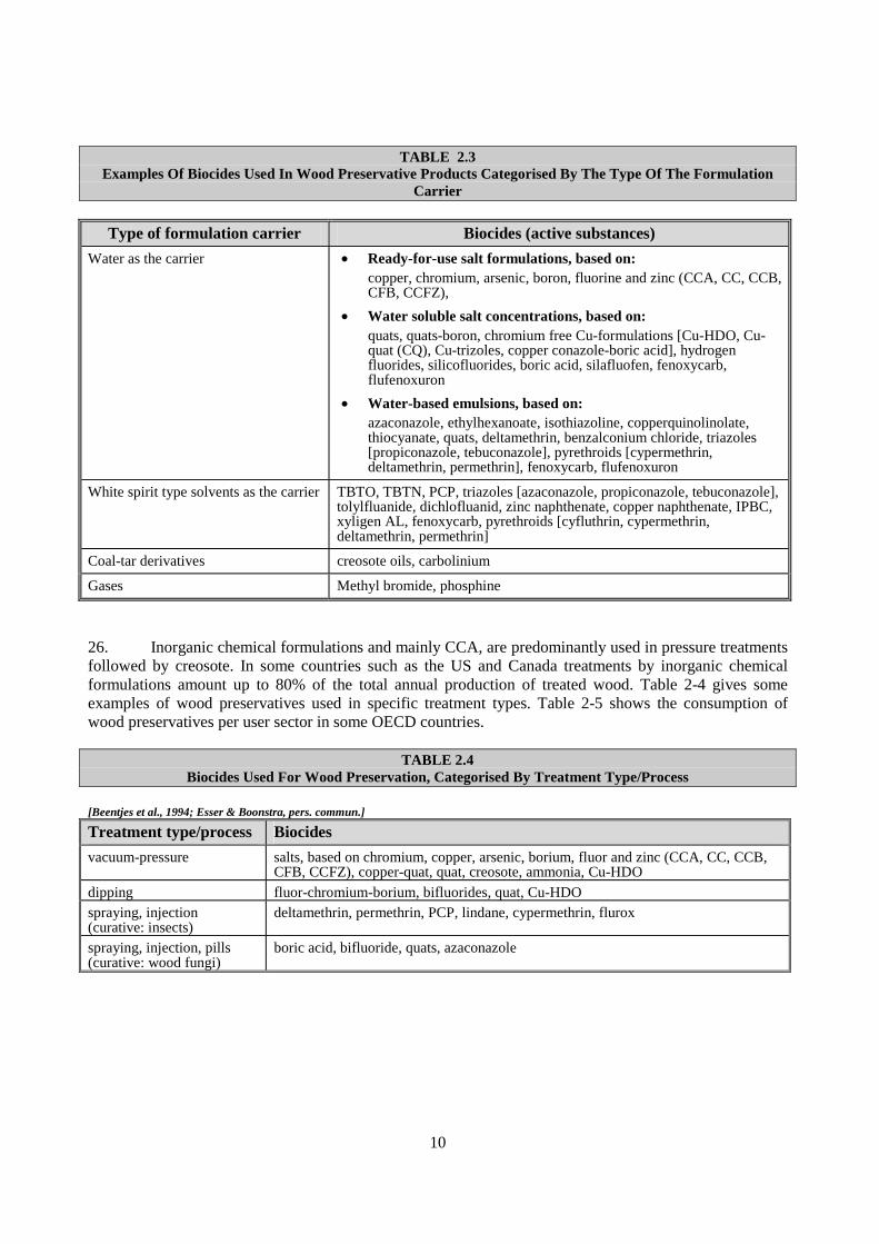
4.2.3 Emission Scenario for Vacuum-Pressure and Double-Vacuum/Low Pressure Processes.........46 4.2.3.1 Process description ............................................................................................................46 4.2.3.2 Environmental Emission Pathways ...................................................................................48 4.2.3.3 Calculation of emissions for Vacuum-Pressure and Double-Vacuum/Low Pressure Treatment 56

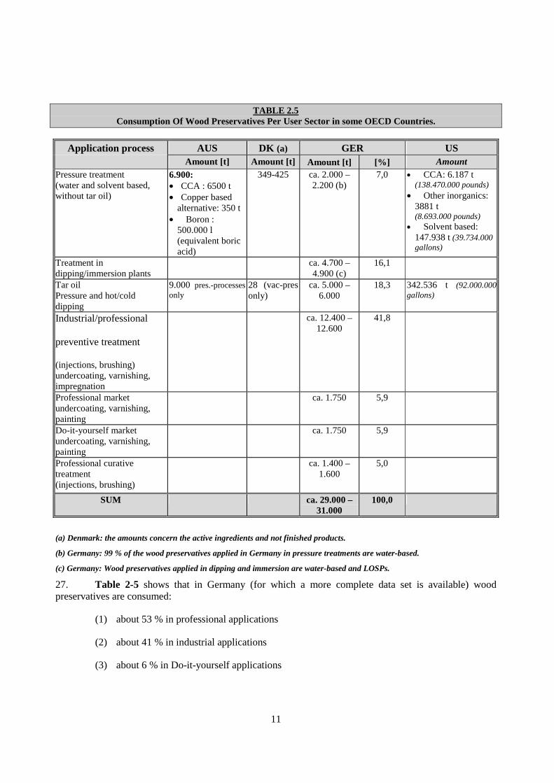
2

FOREWORD

This Emission Scenario Document (ESD) presents an approach to estimate the emissions of wood preservatives from two stages of their life cycle: 1) application and storage of treated wood prior to shipment, and 2) treated wood-in service. This ESD can be used in the estimation of concentrations in the environment of specific active substances used in wood preservatives.

In 1998, OECD Member countries agreed to work together to develop guidance for exposure assessment of biocides in view of the wide variety of exposure scenarios associated with these chemicals. Wood preservatives were selected first for examination because most countries already had experience in regulating them (see OECD Survey of Member Countries’ Approaches to the Regulation of Biocides1).

In 2000, an OECD Workshop, hosted by the European Chemicals Bureau of European Commission was held in Belgirate, Italy to discuss scenarios for the environmental exposure assessment of wood preservatives [OECD 2000d]. The Workshop made a series of recommendations; one was that OECD should develop an environmental Emission Scenario Document for wood preservatives. The document should build on the extensive background documentation for the workshop and provide guidance on how to estimate emissions:

1) during the wood preservative application processes and storage of treated wood prior to shipment; and

2) from treated wood-in-service. By developing this ESD at OECD-level, wide acceptance will help to reduce duplicative efforts made by Member countries and industry and improve the consistency and transparency of exposure assessments.

An Expert Group was formed to develop this Emission Scenario Document. A list of the members of the Expert Group is given in Appendix 9.

In developing this document, the Expert Group used information from a number of sources and, wherever possible, used established scientific data. In some cases, relevant agreed data did not exist and so the Expert Group had to decide on a value to be used – these default values are identified in the document (those for wood-in-service are all listed in Appendix 3) and wherever possible a rationale for the choice is also given. A fundamental issue considered in the development of this ESD was the size of the receiving environmental compartment. There are no agreed scientific criteria for choosing this and, although there was no unity within the Expert Group, most members agreed to use the values proposed by the Secretariat which appear in this document. These default values are not “fixed in concrete” and if users of this ESD have other, more valid values, then these should be used instead.

Because of its size, the draft ESD has been divided into four parts:

• Part 1: Contains the introductory chapters (Chapter 1-3) and also the scenarios to estimate the emissions from the industrial preventive applications (Chapter 4).

• Part 2: Contains Chapter 5 (wood-in-service) and Chapter 6 (Professional and amateur in-situ treatment).

• Part 3: Contains Chapter 7 (Removal processes) and Appendices 1 to 4.

• Part 4: Contains Appendices 5 to 9. 1 Survey of OECD Member Countries’ Approaches to the Regulation of Biocides, OECD Environmental Health and

Safety Publications, Series on Pesticides No.9, ENV/JM/MONO(99)11.

3

1. GENERAL INTRODUCTION

1.1 Background

1. According to recent national and regional legislation2, environmental exposure assessment, is an integral part of the risk assessment of a biocidal product or of an active ingredient for regulatory purposes.

2. Preferably, representative data from well-designed field studies should form the basis for exposure assessment [OECD 2000a]. Although for some existing active substances monitoring data in air, water or soil may be available, for many substances such information is limited or simply non-existent.

3. As for other chemicals, exposure models offer an alternative solution for the estimation of the environmental emissions of the active substances, and other relevant substances in wood preservatives, when good exposure data are lacking.

4. The purpose of this document is to provide guidance on how the emissions of active substances and other relevant substances from wood preservatives to the environment (i.e. into water, soil and air) from two stages of the wood preservative life cycle can be estimated:

1) product application and storage of treated wood prior to shipment, and; 2) treated wood-in-service.

The product application stage covers: 1) industrial preventive wood preservation treatments and 2) preventive or curative treatments performed in-situ by professionals and amateurs including the do-it- yourself individuals.

5. The estimation of the emissions to the various environmental compartments is based on so-called emission scenarios. It is considered that the scenarios included in this document describe reasonable worst-case situations of normal patterns of product use.

6. For the purpose of this document, the definition of the European Committee for Standardisation (CEN, 35th Meeting of CEN/TC 38) for wood preservatives is used, i.e.:

“Wood preservatives are active ingredient(s) or preparations containing active ingredient(s) which are applied* to wood** or wood-based products themselves, or which are applied to non-wood substrates (e.g.

masonry and building foundations) solely for the purpose of protecting adjacent wood or wood-based products from attack by wood-destroying organisms (e.g. dry rot and termites)”.

* by surface treatment (e.g. spraying, brushing) or deep penetrating processes (e.g. vacuum-pressure, double vacuum etc.)

** wood means logs received at the sawmill for commercial use and for all subsequent uses of the wood and wood-based products.

1.2 Rationale for guidance on the environmental exposure assessment to wood preservatives

7. New regulatory systems for biocides, including wood preservatives, have recently been introduced or will soon be introduced in many OECD countries. These new regulations require a comprehensive environmental risk assessment to take place for authorisation decision-making purposes.

2. E.g. the EU Biocides Directive 98/8/EC which came into force in May 2000. The US EPA draft proposals for

antimicrobial data requirements (Part 158W) will be published soon in the Federal Register.

4

8. As for other chemicals, the essential components of a quantitative environmental risk assessment are:

1. an estimate or measurement of the environmental exposure to the substance in question (exposure assessment), and;

2. an estimate of the toxic effects to flora and fauna that the estimated (or measured) exposure might have (effects assessment).

9. The methods for assessing environmental effects of active substances and other relevant substances in wood preservatives will not, in principle, be different from those used for other chemicals. Furthermore, internationally harmonised methods and protocols exist for these purposes. However, no such internationally accepted guidance exists for estimation of the environmental exposure to biocides. As there is a wide variety of exposure scenarios associated with the use of biocides, wood preservatives were chosen as a starting point for the development of such an international guidance. This Emission Scenario Document (ESD) therefore includes methods and approaches for the quantitative evaluation of environmental exposure to wood preservatives.

10. It is expected that the ESD, once finalised and endorsed by the relevant OECD bodies, will help the biocide regulatory agencies in the OECD Member countries to perform exposure assessment to wood preservatives in a consistent way which, in the long term, will allow work sharing among countries in the evaluation of industry’s dossier submissions for product registration. This document may also help chemical producers assessing the potential impact of current and new products, potential users of chemicals comparing alternatives etc. It may also be of use in developing estimates of releases for Pollutant Release and Transfer Registers (PRTPs).

1.3 Life cycle of wood preservatives

11. There has been a marked shift in emphasis in regulatory exposure assessment to take into account the emissions and exposure that results from all stages of a chemical’s life (a ‘cradle-to-grave’ approach): production, formulation, processing, use (service life of treated materials), and recovery or disposal from service to disposal sites (e.g. landfill sites).

12. The life cycle of a wood preservative involves the following stages:

• Production of the active substance is the stage during which the substance is manufactured, i.e. formed by chemical reaction(s) or by biotechnological processes, isolated, purified, drummed or bagged, etc.

• Formulation of preservative is the stage in which substances are combined in a process of blending and mixing to obtain a product or preparation. Formulations are applied or used in the next stage of the life cycle (processing) either as such or diluted in water or organic solvents.

• Product application (Processing): Preventive and curative wood treatment: this stage consists of all kinds of processes whereby the substance as such, a formulation or an article containing the substance is applied or used. Wood preservatives are applied in numerous preventive and curative processes: at industrial scale for preventive purposes before first use of the treated wood, or by professionals and amateurs for preventive and curative treatment of wooden structures in-situ.

5

• Service life: Wood-in-service: this stage considers the service of treated wood. Wood is used in a variety of applications and is often preventively or curatively treated to increase its durability with time. The emissions of wood preservatives to the environment during the service life of treated wood might be considerable especially in view of the long time (up to 50 years) that treated wood is in service.

• Waste treatment: at this stage the unused wood preservative products or the out-of-service treated wood is disposed of with waste. Waste treatment may consist of incineration or landfill dumping. Releases during these processes are considered through leaching models and release of non-degraded substances during incineration, especially heavy metal oxides [Van der Poel 1999; Deutscher Holzschutzverband 1999].

• Recovery: Out-of-service use: This stage comprises secondary uses of out-of-service wood, e.g. railway sleepers in landscaping.

• Contaminated sites can include operational and non-operational treating plants and storage yards for treated wood products. Although contaminated sites have a defined distinct boundary they may release toxic substances to the environment.

13. It is difficult, however, to develop in one single document methodologies for emission estimation for all life stages above. Therefore, this document focuses only on the life cycle stages of 1) product application: preventive and curative wood treatments and 2) wood-in-service. Also, disposal of wastes from treatment plants or disposal of treated wood after service do not fall under the scope of this document.

1.4 Structure of the document

14. This document is structured as follows:

Chapter 2: gives a brief overview of the main treatment types and processes, main wood preservative product types and main uses of treated wood.

Chapter 3: briefly describes the principles of exposure assessment which is a part of risk assessment; clarifies the focus of this document regarding the calculations proposed; and describes the approach followed to identify representative scenarios for each life stage which were needed as a basis for the calculations.

Chapter 4: describes three scenarios selected for estimation of the emissions from industrial preventive applications and proposes calculations of the emissions.

Chapter 5: describes the scenarios selected for estimation of the emissions during the service life of industrially pre-treated wood and proposes calculations of the emissions.

Chapter 6: describes the scenarios selected for estimation of the emissions from preventive and curative in-situ treatments, performed by professionals and/or amateurs. The calculations proposed cover emissions during these treatments (i.e. product application stage) and after them (i.e. wood-in-service stage).

Chapter 7: describes a more elaborated approach to calculate the emissions from treated wood as a function of time and takes into account removal processes of the substance (such as degradation, volatilisation, leaching to ground water etc) in the environmental compartments of concern.

6

2. MAIN TREATMENT TYPES, PRODUCT TYPES AND USES OF TREATED WOOD

2.1 Main treatment types and processes

15. Wood is used in a variety of applications and depending on the type of wood and the type of use site (e.g. underwater, in houses), it can be affected by insects or fungi. To counter organisms that challenge and destroy it, wood is treated with preservatives at either or both of two distinct stages in its ‘life cycle’:

• preventively to prevent or retard the occurrence of biological degradation by fungi, bacteria and wood-boring insects (including termites and marine borers) on wood; and

• curatively (remedial) to remedy infestations once they have occurred, either in previously treated wood or in wood that has never been treated.

16. The application of wood preservatives is performed at various scales and with various techniques:

• Preventative treatments are usually applied at industrial scale operations to wood before the wood is put into service (although professionals and amateurs also preventatively treat wood structures in-situ). In the industrial operations, the type of treatment and the active substances applied relate to the anticipated use of the wood, and the potential for decay or insect infestation. Protection against biological degradation or disfiguration in some environments can be controlled through simple surface treatments such as spraying and dipping; other situations require that the preservative penetrates wood more deeply and therefore vacuum or pressure and vapour impregnation is appropriate.

In most cases, the wood for preservation has been shaped as a “wood product” for later assembly. Subsequent working of treated wood is generally low, being limited to sawing, planing or sanding at the site where it is to be assembled or installed.

• Curative treatments (remedial) are applied to wood in-situ by professionals or amateurs including the do-it-yourself fans. The treatment can involve initially work for removing decorative coatings, flooring or ceilings. This allows to determine the extent of the damage and to apply the remedial product where it is needed, for example, by spraying, brushing or injections. Smokes or fumigant gases without extensive site preparation can treat some insect infestations.

Further general information on wood preservatives can be found in chapter 8 of “The Biocides Business”(72)

7

17. An overview of the treatment types and processes is given in Table 2-1.

TABLE 2-1 Overview Of The Preventive And Curative Treatments Of

Wood With Wood Preservatives.

Type User sector* Preservation process Preventive Sawmills (industrial) • automated spraying • automated dipping ‘Heavy-duty’ industrial

preservation • vacuum-pressure process • thermal impregnation process • vapour process

‘Joinery’ industrial preservation

• double-vacuum process • deluge / flood process • dipping process (mechanised or manual) • spraying process

Professional in-situ • spraying treatments • injection; injection in soil; pills • wrapping • brushing Amateurs • brushing

• spraying Curative Professionals • fumigation, injection, pills, wrapping, spraying Amateurs • brushing, spraying

*In-situ temporary antisapstain treatment of freshly felled logs is not considered a wood preservation process for the purpose of this document.

18. In Australia, North America (Canada and US) and some European countries (such as Denmark), the majority of the wood is treated preventively at industrial scale with vacuum-pressure processes. The picture is different in other European countries, such as Germany, where preventive surface treatments (e.g. immersion, brushing) and injection at the small professional enterprise scale, are the predominant methods used. Table 2-2 shows the number of industrial treating plants by process for some OECD countries.

8

TABLE 2.2 Number Of Wood Preserving Plants By Process In Some Oecd Countries

(AUS: Australia; CAN: Canada; DK: Denmark; GER: Germany; NL: Netherlands; UK: United Kingdom; US: United States)

Number of plants Industry branch Process

AUSa CAN

b DK

c GER

d NL

e UK

f U

Sg

Surface treatments Sawmill Immersion, dipping 5 no data no data ca. 920

Sawmill Spraying 5 no data no data Joinery, carpentry Immersion, dipping 5 no data no data 1.500 –

2.100

Others appling hot/cold immersion

Hot/cold immersion no data no data no data 20

Deep penetrating treatments Vacuum-Pressure plants (no creosote)

Vacuum-Pressure

109-121h ≈ 60 21 pressure 64 vacuum

2 masts+poles

300 16 ≈300 (CCA)

451

Vacuum-Pressure plants (creosote)

Vacuum-Pressure

4 ≈ 7 Nil 10-15 3 5

Joinery Double vacuum no data no data no data < 20 ≈500 (notes on following page)

1. AUS: Source: Harry Graves and Terry Hawkins, response to the OECD questionnaire on industrial preventive applications, January 2001 [reference OECD 2001a].

2. CAN: Source: Henry Walthert, response to the OECD questionnaire on industrial preventive applications, April 2001 and ‘Strategic Options for the Management of Toxic Substances’, Environment Canada, July 1999.

3. DK: Source: Danish Impregnation Control, 1997.

4. GER: Source: Report of Fresenius Umwelt Consult “Gutachten zur Erhebung struktureller Daten ueber industrielle und gewebliche Anwender von Holzschutzmitteln in Deutschland’ (FKZ 360 04 008) February 2001 [UBA 2001].

5. NL: Source: Vereniging van Houtimregneerbedrijven in Nederland (Association of Wood Impregnation Companies in the Netherlands). At least 16 vacuum-pressure plants, all using inorganic wood preservatives (salts). Three of them also use creosote.

6. UK: Source: Health and Safety Executive, September 2001.

7. US: Source: Reference [US EPA 1999].

8. AUS: 90 – 100 CCA; 8 – 10 Copper based alternative waterbornes; 11 Light Organic Solvent Preservative (LOSP); 4 Creosote / Heavy Oil [reference OECD 2001a].

9

2.2 Main wood preservative product types

19. For many years industrial wood preservatives were categorised into:

• inorganic or salt based using water as the carrier for the active substances;

• LOSP (light organic solvent) based using white spirit or petroleum distillate as the carrier for the active substances;

• distillates from coal tar including creosote and pentachlorophenol in heavy oil.

20. The inorganic wood preservatives included formulations based on chromated copper arsenate (CCA), copper chromium boron (CCB) and copper chromium fluorine (CCF). In the last decade products such as copper formulated with combinations of different azoles, ACQ (ammoniacal copper quats) and Copper HDO have all been introduced as alternatives to the traditional inorganic wood preservatives. These all use water as the carrier. It should be noted that the use of the term “inorganic” is now used less and less in the industry.

21. LOSP (also known as organic wood preservatives) formulations historically used active substances such as pentachlorophenol, TBT based compounds, zinc carboxylates, dieldrin and lindane. Today’s LOSP products are formulated around mixtures of azoles such as propiconazole and tebuconazole with IPBC, permethrin and cypermethrin.

22. In the last decade many of the treatments previously using LOSPs have changed to emulsion formulations using combinations of azoles, IPBC, quaternary ammonium compounds, cypermethrin and permethrin using water as the carrier. Borates have also been used with water as the carrier.

23. In addition to the wood protection properties imparted to the timber, very often the products are formulated to give additional properties to the treated timber such as water repellence and colour.

24. Inorganic (or salt based) chemical formulations can be divided in fixating and non-fixating, based on the interactions with the wood. Fixating biocides are chemically bound to the wood (chemical reaction). An overview of reactions of CCA salts with wood is presented in [Berbee RPM, 1989)]. Non-fixating biocides have a strong diffusive capacity; wood impregnated with this type of preservatives has to be equipped with a paint or lacquer layer, to prevent intensive leaching [Beentjes et al., 1994]. Inorganic chemical formulations (with water as a carrier) generally leave the wood surface clean, paintable, and free from odour. Solvent-based preservatives and coal-tar distillates do not react with the wood, but are bound by hydrophobic interactions.

25. The number of active substances used in wood preservation is very extensive. Most biocide substances are either insecticides or fungicides, and therefore wood preservatives contain usually mixtures of substances. Boric acid and arsenic are exceptions as they act as both insecticide and fungicide. Pyrethroids (replacements of lindane) are typical insecticides. Quats and triazoles are typical fungicides. The broad scope of working with creosote is a result of the composition (many different PAH, each with a more or less specific effect). Table2-3 gives examples of biocides (i.e. active substances) used in wood preservative products categorised by the type of the formulation carrier (i.e. water or oil/solvent).

10

TABLE 2.3 Examples Of Biocides Used In Wood Preservative Products Categorised By The Type Of The Formulation

Carrier

Type of formulation carrier Biocides (active substances)

Water as the carrier • Ready-for-use salt formulations, based on: copper, chromium, arsenic, boron, fluorine and zinc (CCA, CC, CCB, CFB, CCFZ),

• Water soluble salt concentrations, based on: quats, quats-boron, chromium free Cu-formulations [Cu-HDO, Cu-quat (CQ), Cu-trizoles, copper conazole-boric acid], hydrogen fluorides, silicofluorides, boric acid, silafluofen, fenoxycarb, flufenoxuron

• Water-based emulsions, based on: azaconazole, ethylhexanoate, isothiazoline, copperquinolinolate, thiocyanate, quats, deltamethrin, benzalconium chloride, triazoles [propiconazole, tebuconazole], pyrethroids [cypermethrin, deltamethrin, permethrin], fenoxycarb, flufenoxuron

White spirit type solvents as the carrier TBTO, TBTN, PCP, triazoles [azaconazole, propiconazole, tebuconazole], tolylfluanide, dichlofluanid, zinc naphthenate, copper naphthenate, IPBC, xyligen AL, fenoxycarb, pyrethroids [cyfluthrin, cypermethrin, deltamethrin, permethrin]

Coal-tar derivatives creosote oils, carbolinium

Gases Methyl bromide, phosphine

26. Inorganic chemical formulations and mainly CCA, are predominantly used in pressure treatments followed by creosote. In some countries such as the US and Canada treatments by inorganic chemical formulations amount up to 80% of the total annual production of treated wood. Table 2-4 gives some examples of wood preservatives used in specific treatment types. Table 2-5 shows the consumption of wood preservatives per user sector in some OECD countries.

TABLE 2.4 Biocides Used For Wood Preservation, Categorised By Treatment Type/Process

[Beentjes et al., 1994; Esser & Boonstra, pers. commun.]

Treatment type/process Biocides

vacuum-pressure salts, based on chromium, copper, arsenic, borium, fluor and zinc (CCA, CC, CCB, CFB, CCFZ), copper-quat, quat, creosote, ammonia, Cu-HDO

dipping fluor-chromium-borium, bifluorides, quat, Cu-HDO spraying, injection (curative: insects)

deltamethrin, permethrin, PCP, lindane, cypermethrin, flurox

spraying, injection, pills (curative: wood fungi)

boric acid, bifluoride, quats, azaconazole

11

TABLE 2.5

Consumption Of Wood Preservatives Per User Sector in some OECD Countries.

Application process AUS DK (a) GER US Amount [t] Amount [t] Amount [t] [%] Amount

Pressure treatment (water and solvent based, without tar oil)

6.900: • CCA : 6500 t • Copper based

alternative: 350 t • Boron :

500.000 l (equivalent boric acid)

349-425 ca. 2.000 – 2.200 (b)

7,0 • CCA: 6.187 t (138.470.000 pounds)

• Other inorganics: 3881 t (8.693.000 pounds)

• Solvent based: 147.938 t (39.734.000 gallons)

Treatment in dipping/immersion plants

ca. 4.700 – 4.900 (c)

16,1

Tar oil Pressure and hot/cold dipping

9.000 pres.-processes only

28 (vac-pres only)

ca. 5.000 – 6.000

18,3 342.536 t (92.000.000 gallons)

Industrial/professional

preventive treatment

(injections, brushing) undercoating, varnishing, impregnation

ca. 12.400 – 12.600

41,8

Professional market undercoating, varnishing, painting

ca. 1.750 5,9

Do-it-yourself market undercoating, varnishing, painting

ca. 1.750 5,9

Professional curative treatment (injections, brushing)

ca. 1.400 – 1.600

5,0

SUM ca. 29.000 – 31.000

100,0

(a) Denmark: the amounts concern the active ingredients and not finished products.

(b) Germany: 99 % of the wood preservatives applied in Germany in pressure treatments are water-based.

(c) Germany: Wood preservatives applied in dipping and immersion are water-based and LOSPs.

27. Table 2-5 shows that in Germany (for which a more complete data set is available) wood preservatives are consumed:

(1) about 53 % in professional applications

(2) about 41 % in industrial applications

(3) about 6 % in Do-it-yourself applications

12

It shows further that:

(1) about 95 % are applied in preventive treatment

(2) about 5 % in curative treatment.

28. Wood preservatives include biocides that are currently available on the market, and biocides that have been available in the (recent) past; this is because of the long time during which preserved wood is used (up to 50 years). Some wood preservatives, although widely used in some countries, have been banned in others. For example, in Denmark and in Switzerland, arsenic is banned (even for imported wood). In Denmark creosote and chromium have been banned for wood preservation since 1998 but they are still allowed in imported wood. In the Netherlands, creosote treated wood is allowed for railway sleepers and for use in the agricultural and garden sector, but not for wood in contact with water. In Germany tar oil wood preservatives are prohibited for private and in-house use. In countries such as the US and Canada, almost 80% of the pressure-treated wood is treated with CCA (copper chrome arsenic). In Australia, although most of the pressure plants use CCA and not creosote, the annual consumption of creosote is 9.000 tonnes compared to 6.500 tonnes of CCA. In Germany the major heavy duty wood preservatives (i.e. preservatives used for deep penetrating processes such as pressure treatments) are CCB and CCF while in the last 10 years products without chromium such as Cu-HDO, Cu-quat, Cu-triazol have been increasingly used. Generally in Europe, lindane, PCP, mercury compounds and arsenic-compounds (except for CCA salts for vacuum-pressure impregnation) are prohibited.

2.3 Main uses of treated wood

29. Wood is used in a variety of applications, from house fronts to bank revetments. Table 2-6 provides some examples of wooden commodities categorised by use site.

TABLE 2.6 Applications Of Treated Wood

Use site Examples of wooden commodities

Indoors various, roof trusses

Outdoors house fronts (claddings) roof tiles window frames playing tools garden houses fences

landings, wharves bridges bank revetment sound-proof barriers railway sleepers telephone poles fence poles car pools wood in gardens use of treated timber in flood defences (UK)

13

30. In terms of the type of wood product treated, both consumer products (e.g. consumer lumber, plywood) and industrial products (utility poles, railway ties etc) are treated. In the US, the most commonly treated product in 1995 was lumber3, which accounted for 43,4 percent of the total volume treated, followed by timber4 (12,8 percent), cross ties (12,8 percent), and poles (11,9 percent). The situation in Canada for the same year was similar: consumer lumber was the single major use (48,7 percent) of the total volume treated, followed by utility poles (18 percent), industrial lumber and timber (14 percent), and railway ties crossties (10 percent). Table 2-7 summarises the production of treated wood by wood products in the US in 1995 [US EPA 1999]. Table 2-8 provides the consumption of wood preservation biocides by treated wood uses in Germany in 1992.

TABLE 2-7 Production Of Treated Wood In The United States In 1995

Volume of wood treated, 1.000 ft3 (to convert in m3, 1 ft3 = 0.028 m3)

Product

Creosote

solutiona

Oilborne

preservativesb

Waterborne

preservativesc

Fire retardants

Total

Crossties 69.947 0 4.177 0 74.124 Switch and bridge ties

6.125 360 2.647 0 9.132

Poles 8.941 30.617 29.215 0 68.773 Piling 1.415 0 7.820 0 9.235 Fence posts 244 339 18.204 0 18.787 Lumber 1.810 320 247.436 1.714 251.280 Timber 1.754 77 72.031 0 73.862 Plywood d 3 16.528 2.049 18.580

Othere 1.515 1.048 52.538 0 55.101

Total 91.751 32.764 450.596 3.763 578.874

a) Creosote, Creosote-coal tar, and Creosote-petroleum.

b) Copper naphthenate, Pentachlorophenol, and others.

c) Chromated copper arsenate (CCA), Ammoniacal Copper Zinc Arsenate (ACZA), Acid Copper Chromate (ACC), Ammoniacal Copper Quat (ACQ), and others.

d) Included in “other” category.

e) Includes cross arms, landscape timbers, highway posts and guard-rails, mine ties and timbers, crossing planks, and other miscellaneous products.

TABLE 2.8 Use Of Wood Preservation Biocides In Germany, Differentiated To Purpose

Salts (tons) Coal tar (tons) Other (tons)

Construction 3.200-5.000 - 5.100-7.600

Outdoors use 3.200-4.300 15.000 3.100-4.300

Others 600-700 - 800-1.100

3 Lumber: wood that has been cut into a finished product. 4 Timber: rough-sawn wood that has not been formed into a finished product, i.e. logs.

14

3. PRINCIPLES OF ENVIRONMENTAL RISK ASSESSMENT FOR WOOD PRESERVATIVES

3.1 Stages of risk assessment

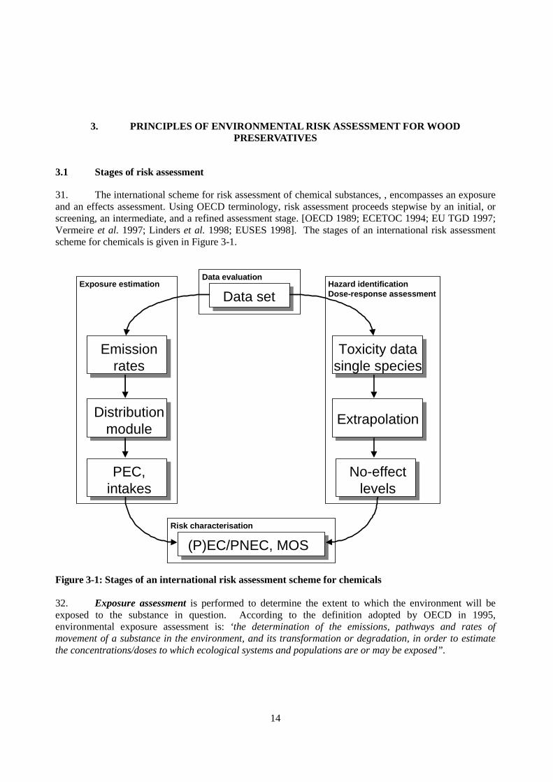
31. The international scheme for risk assessment of chemical substances, , encompasses an exposure and an effects assessment. Using OECD terminology, risk assessment proceeds stepwise by an initial, or screening, an intermediate, and a refined assessment stage. [OECD 1989; ECETOC 1994; EU TGD 1997; Vermeire et al. 1997; Linders et al. 1998; EUSES 1998]. The stages of an international risk assessment scheme for chemicals is given in Figure 3-1.

Figure 3-1: Stages of an international risk assessment scheme for chemicals 32. Exposure assessment is performed to determine the extent to which the environment will be exposed to the substance in question. According to the definition adopted by OECD in 1995, environmental exposure assessment is: ‘the determination of the emissions, pathways and rates of movement of a substance in the environment, and its transformation or degradation, in order to estimate the concentrations/doses to which ecological systems and populations are or may be exposed”.

Data evaluation

Data set

Risk characterisation

(P)EC/PNEC, MOS

Exposure estimation

Emissionrates

Distributionmodule

PEC,intakes

Hazard identificationDose-response assessment

Toxicity datasingle species

Extrapolation

No-effectlevels

15

33. Preferably, representative data from well-designed field studies should form the basis for exposure assessment. However, such data are not available in many cases and exposure models offer an alternative solution to estimate the exposure.

34. According to the latter approach, emissions to water, soil and air during the substance's life-cycle are first estimated, along with the dispersion of the substance in the compartments (including sediments). This makes it possible to predict, subsequently, the concentration of the substance in the environment, known as the Predicted Environmental Concentration, or PEC.

35. Effects assessment is performed to estimate the toxic effects to flora and fauna that the estimated (or measured) exposure might have. After the environmental concentration has been determined, a dose-response assessment is performed on the basis of laboratory test results for several end-points (e.g. aquatic organisms, terrestrial organisms, micro-organisms in the sewage treatment plant and top predators such as fish-eating and worm-eating birds or mammals). The dose-response assessment generally derives concentrations at which no adverse effects are expected, known as the Predicted No Effect Concentration or PNEC.

36. Together, the exposure assessment and the effects assessment lead to a risk assessment that reaches a conclusion about the likelihood of adverse effects in the exposed population. This is done by calculation of Risk Characterisation Ratios (RCR) such as PEC/PNEC for the various ecosystems to be protected. Further general information on wood preservatives can be found in chapter 7 of “The Biocides Business”(72)

3.2 Environmental exposure assessment

37. In general, environmental exposure assessment has to describe which organisms or ecosystems are exposed to a substance via which route and to which extent. Thus, the concentration of a substance in all environmental compartments, the frequency and the duration of exposure are important components of exposure assessment.

38. The estimation of a substance’s concentration in an environmental compartment includes two steps:

• Emission estimation: the pathways that the emissions enter to the relevant environmental compartment during the different stages of a product’s life have to be identified and the quantity of the emissions to be estimated. This can be done based on so-called emission scenarios that are developed for each life stage of the product. OECD defines an emission scenario [OECD 2000b] as a set of conditions about emission sources and pathways, production processes and use patterns that quantify the emissions of a chemical from the different stages of its life cycle.

• Distribution estimation: the distribution of the substance in the environmental compartment of concern is estimated at appropriate spatial scale and time. To this end, models take into account the physical chemical properties of the substance and its degradation, transport and partitioning between the different compartments.

16

3.3 Spatial scales

39. The risk that wood preservatives and treated wood might present for the environment depends upon the size of the affected environment. The EU Technical Guidance Document for risk assessment of chemicals [EU TGD 1997] refers to continental, regional and local environments which are specified as follows :

TABLE 3.1 Size Of The Environment For Environmental Risk Assessment According To The EU TGD

Spatial Scale Value

Continental (Europe) 3.56E+06 km2

Regional 200 km * 200 km

Local 100 m from the source (air)

Local 1000 m from the source: deposition on soil

40. In the risk assessment regimes of US and Canada, the size of regional and continental is not specified with numbers but regional and continental exposure is considered when multi-source local exposure assessments indicate a risk for exposure at such scales.

41. In the case of wood preservatives, releases from point sources (e.g. a treatment plant) have an impact on the local scale and also contribute to the regional scale. Environmental risk assessment for treated wood-in-service has to consider smaller local environments than the local environments considered for industrial treatment plants. Baines and Davis (1998) cited the following possible local environments for environmental concentrations due to leaching from treated wood-in-service.

TABLE 3.2 Suggested Size Of The Environment For Risk Assessment For The Life Stage Of Treated Wood-in-service

Spatial Scale Value Local 100 m from the source (air)

Adjacent 10 m from the source (water)

Surface 10 cm from the source (soil)

3.4 Time scale

42. Generally, in exposure assessment, three distinct time scales for the environmental concentrations of the substance of concern are used in respect to the ecotoxicological acute and chronic time scale.

• initial concentrations: these are concentrations immediately after the last application (e.g. at the end of the application day); any degradation processes are not considered (worst-case).

• actual concentrations: these are concentrations after a certain time (days) has elapsed. Environmental degradation processes affect such concentrations.

• time average concentrations: these are concentrations that are averaged over a certain time period. Such concentrations are necessary, when long-term effects are considered.

17

3.5 Focus of the document

43. This document focuses only on the exposure assessment and specifically the estimation of local emissions to the various primary receiving environmental compartments from only two stages of a wood preservative life cycle, i.e.:

• product application:

- industrial preventive treatments including storage prior to shipment

- professional and amateur in-situ treatments (preventive and curative)

• treated wood-in-service

Calculations of the local concentrations (Clocal) in the receiving compartments are also proposed but only for the life stages of:

• storage of industrially treated wood prior to shipment

• treated wood-in-service

• product application during in-situ preventive or curative treatments

44. The methodologies, proposed in this document, apply to any active ingredient or any substance of concern in a wood preservative product.

Estimation of local emissions during product application

45. Local emissions during industrial and professional and amateur treatments in-situ, are considered within one day. The term used in these cases is ‘local emission rate (Elocal)’ and is expressed as the mass of the substance emitted to an environmental compartment at a local scale per day. Industrial processes are considered to be continuous, while in-situ treatments are considered discontinuous.

46. These emissions rates (i.e. Elocalair or Elocalfacilitydrain expressed in kg.d-1) can then be used further in exposure assessment as input values in atmospheric diffusion models, sewage treatment models or surface water models. These kind of models are an integral part of all national risk assessment schemes and need not to be mentioned here. Screening models have also been proposed by the OECD [OECD 1992].

Estimation of local emissions from treated wood during storage and during service life

47. Local emissions from industrially treated wood during storage prior to shipment are described as ‘the cumulative quantity (Qstorage) of a substance emitted from the stored treated wood over a certain assessment period’. Qstorage is expressed in mass [kg]. In this case local emissions and concentrations are considered within two different time windows proposed by the Expert Group, based on Belgirate Workshop recommendations [OECD 2000c]:

• 30 days for an initial assessment

• 30 days for a longer assessment period

48. Local emissions from treated wood-in-service are described as ‘the cumulative quantity (Qleach) of a substance emitted from treated wood to an environmental compartment at a local scale within a certain time period of service (i.e. the assessment period)’. Qleach is expressed in mass [kg]. In this case, local emissions and concentrations are considered within the same time windows for the service life as for storage:

18

• over the first 30 days of the service life

• during the rest of the service life (> 30 days)

49. The 30 day cut-off was selected in order to be coherent with a typical life-cycle period of soil or water organisms.

Estimation of local concentrations

50. For the specific life stages of treated wood during storage and during service life and of in-situ product application, proposals for calculation of local concentrations (Clocal) in the relevant primary receiving environmental compartments are made. The time spans considered for these calculations are the same as for the calculation of the local emissions in each respective case. Two options for calculation of Clocal are proposed:

• one option which does not take into account removal processes of the substances emitted from the receiving compartment due for example to degradation, volatilisation, leaching to ground water etc., (relevant Sections in Chapters 4, 5 and 6)

• first tier methods for taking into account environmental behaviour of a substance in the receiving compartment (Chapter 7)

51. The Clocal, estimated according to the methodologies proposed in this document for treated wood-in-service may be used for the following time scales in an exposure assessment scheme (for example for the PEC calculation):

• initial concentrations: these are concentrations immediately after the last application (e.g. at the end of the application day)

• short-term concentrations: These are concentrations over the first 30 days that emissions occur. This time window covers the initial leaching, and it is similar to the duration of chronic ecotoxicity test that are used for derivation of the PNEC

• long-term concentrations : these are concentrations over a period of time > 30 days. Depending on the characteristics of the active ingredients and the service life of treated commodities, time periods of several years of service life can be used

Estimation of concentrations in ground water

52. Although the document is focused on emissions and concentrations to primary receiving environmental compartments, it provides some guidance on how potential emissions to ground water via leaching of a substance in soil can be calculated (Appendix 4). Two models (i.e. PEARL and PELMO), initially designed for prediction of the leaching of a substance in soil for agricultural pesticides, are discussed with respect to their applicability in the scenarios for treated wood-in-service and storage prior to shipment, for calculation of the emissions from treated wood that may reach ground water.

19

3.6 Selection of emission scenarios

53. To estimate the emissions, appropriate ‘emission scenarios’ had to be identified and fully described for each of the two life stages of wood preservatives, covered by this document. The selection of the scenarios in this document is based on the Belgirate workshop recommendations [OECD 2000c].

3.6.1 Scenarios for the life stage of product application

54. As Table 2-1 shows, wood preservatives are applied by many different processes and techniques. These can be grouped into two major categories:

• industrial preventive applications

• professional and amateur in-situ treatments (preventive and curative)

55. The industrial preventive applications, identified as most important in terms of usage in OECD member countries and exposure potential, are:

• Spray tunnels/deluging (surface treatment processes)

• Immersion/dipping (surface treatment processes)

• Pressure processes: Vacuum-pressure or double vacuum/low pressure (deep penetration processes)

Therefore, the scenarios proposed in Chapter 4 for estimation of the emissions during the application stage are built on these processes.

56. The professional and amateur in-situ (curative and preventive) treatments, identified by the Belgirate workshop as the most common in the OECD member countries, are:

• Spraying (indoors)

• Brushing (indoors and outdoors)

• Fumigation (indoors)

• Injection (indoors/outdoors)

• Wrapping (outdoors), and

• Foundation preventive treatment against termites.

57. The Expert Group found it more appropriate that the selection of the scenarios to estimate emissions from these treatments be based on the use site (indoors or outdoors) and on the wooden commodities treated by these techniques, rather than on the basis of the application techniques as done for industrial applications. The scenarios proposed in Chapter 6 are used to estimate both the emissions during these treatments (i.e. product application stage) and after them (i.e. wood-in-service stage).

3.6.2 Scenarios for the life stage of wood-in-service

58. As for in-situ treatments described above, the selection of the scenarios to estimate the emissions during the service life of industrially pre-treated wood is based on the use site (indoors or outdoors) and on the wooden commodities made of such wood. These scenarios are described in Chapter 5.

20

4. EMISSION ESTIMATION FOR INDUSTRIAL PREVENTIVE PROCESSES

4.1 General considerations

59. In all three emission scenarios for preventive industrial processes (i.e., automated spraying, dipping/immersion and pressure processes), the emissions to the various environmental compartments are considered to occur during the:

1) treatment process including post-treatment conditioning, and;

2) storage of treated wood prior to shipment.

60. Emissions generated from the waste of the treatment plants, such as sludge from dipping baths; contaminated sawdust and; waste timber, are not considered in this document because many OECD countries have specific legislation for the disposal of such waste.

61. For example, the European Waste Catalogue (EWC) [Commission Decision 94/3/EC of 20 December 1993; OJ No L5, 7.1.1994, p. 15] is presently being replaced and covers the following waste categories concerning wood preservatives. These waste categories are considered as hazardous waste pursuant to Article 1(4) of European Council Directive 91/689/EEC of 12 December 1991 (OJ No. L377, 31.12.1991, p. 20) based upon European Council Directive 75/442/EEC on waste [OJ No. L78, 26.03.1991, p.32]. In Canada the wastes from wood preservation plants are classified under the federal Transport of Dangerous Goods regulations as hazardous wastes and therefore have strict requirements for shipment and handling. Canadian provinces also classify these wastes as hazardous and regulate the way(s) that they can be disposed of in Canada. This typically requires that they be sent to a ‘secure landfill’.

TABLE 4.1 European Waste Categories for Wood Preservatives

Waste category Description 03 02 wood preservation wastes

03 02 01 non-halogenated organic wood preservatives

03 02 02 organochlorinated wood preservatives

03 02 03 organometallic wood preservatives

03 02 04 inorganic wood preservatives

4.1.1 Post-treatment conditioning

62. Post-treatment conditioning is considered as a part of the treatment process. It is the period of time following the withdrawal of the freshly treated timber from the treatment installation (all methods of application) to allow the preservative to be firmly bound to the wood. Depending on the process, post-treatment conditioning can take place in the containment area of the treatment installation or outside it.

21

63. During this period various processes take place in the treated wood. Depending on the wood preservative formulation used, these processes may include one or more of the following:

• Evaporation of the carrier, water or solvent;

• Breaking of the emulsion;

• Deposition of the active substance in or on the wood;

• Fixation of the active substance by chemical or other means with the wood substrate. Fixation is a term originally used for chromium containing preservatives;

• Other processes that lead to the resistance to leaching of the active substance out of the treated timber.

64. The post-treatment conditioning period may be shortened by the use of accelerated fixation techniques, elevated temperatures, or increased ventilation. For example, an accelerated fixation technique applied to freshly treated timber with inorganic chemical preservatives (such as CCA) is low-pressure steam (105°C). Steam treatment is also used after impregnation with creosote to remove low molecular PAHs, to reduce leaching during use. Another technique to fixate the preservative is 'diffusion'. The treated wood is covered or sealed in plastic foil, and stored, to facilitate diffusion in the wood.

65. Providing that climatic conditions allow it, "natural" fixation by storing the impregnated wood for 4 to 12 weeks (average: 6-8) gives the best fixation results, in terms of reduction of leaching during use [Esser & Boonstra, personal communication.].

4.1.2 Storage of treated wood prior to shipment

66. This is the period when the treated timber is stored after the post-treatment conditioning phase while waiting for shipment. The storage conditions of the treated timber can vary considerably; it can be under cover and/or paved (as it is usually in the case of high value joinery products) or exposed to the weather.

67. Treated timber stored in a manner where it is exposed to the elements, such as rainfall, represents a potential for emissions from the treated wood to take place. On terrain with a paved base surface, the water can be collected, recycled or treated on site. However, on terrain without special base protection, the water carrying the biocides can penetrate the soil, causing soil contamination and subsequent risks for ground and surface water. Emissions to surface water may also occur directly via rain run-off.

68. Examples of estimated emissions, based on experimental data, from pressure-treated wood during storage are provided in Section 4.2.3.2.

69. The storage scenario proposed in this document assumes that the storage area is uncovered and unpaved. It is considered that this scenario represents a realistic worst-case for several OECD countries, as it was pointed out at the Belgirate Workshop [OECD 2000c]. The regulatory authorities and exposure assessors may refine it, if they know the specific situation for their country with respect to storage.

22

4.1.3 Environmental compartments exposed and emission pathways

70. In all three scenarios proposed in this Chapter, the environmental compartments, considered to potentially receive emissions, are:

• from the process (including post-treatment conditioning):

- outdoor air

- facility drain. The emissions to the facility drain may enter in surface water via a public sewage treatment plant (STP) (Note that not all treatment plants are directly connected to a facility drain, however).

• from the storage (when storage area is uncovered and unpaved):

- soil due to leaching from treated wood via rainfall, and ground water via leaching of the substance in soil;

- surface water via rain run-off.

71. Table 4.2 provides an overview of the potentially exposed environmental compartments for all three scenarios of industrial preventive applications.

TABLE 4.2 Environmental Compartments Potentially Exposed From Industrial Preventive Applications

Application/Scenario Process Storage (when uncovered, unpaved)

Air (outdoors)

Waste water Surface water Soil Ground watera

Surface water

1. Automated spraying + + + + + + 2. Immersion/dipping

(small and large scale)

+ + + + + +

3. Vacuum-pressure & Double vacuum/Low pressure

+ + + + + +

a Indirect exposure via leaching of the substance in soil

72. It should be noted, however, that some of the emission pathways and environmental compartments considered here may not apply in certain countries. In most countries, wood treating plants need to be authorised by government authorities according to environmental laws or regulations. These regulations may prescribe in detail the required design of a new plant in order to get authorisation for operation. In addition industry associations have issued ‘Best Practice Guides for Treating Plants’ that provide instructions for environmental best practices including contamination of sites and surroundings. The status of these guides is voluntary in most countries but the guides are usually recognised and used by the authorities responsible for the authorisation of plants. Table 4-3 provides information on such guides in some OECD countries.

23

73. However, it should be noted that the strictness and enforcement of the above regulations vary among countries. Among the numerous industrial processes for treating wood, pressure plants are the most strongly regulated and they generally operate with modern technology and design. In Canada, Switzerland and UK, regulations for pressure plants require that they are roofed and built upon sealed flooring with no connection to the facility sewer system (facility drain), and storm rainwater should be collected and be united with the tank treating solution. However, it is questionable whether older plants are in compliance with new and stricter regulations for their operation. In Canada, all the 67 heavy-duty treatment plants currently in operation were audited by Environment Canada in 2000. The overall compliance levels were: for CCA - 65%, for creosote - 69%, for PCP – 68% and for PCPT 78%.

TABLE 4.3 Best Practice Guides For The Operation Of Industrial Wood Treating Facilities In Some OECD Countries

Country Guide Australia • Australian Standard 2843 (Timber Preservation Plant Safety Code): This standard is a

guidance only, however, compliance with this standard is increasingly embedded in EPA statutory licence requirements.

• Australian Environmental Guidelines for CCA Preservation Plants: Comment as per AS 2843.

Canada Technical Recommendations Document for the Design and Operation of Wood Preservation Facilities, [Brudermann GE 1999]. Currently the TRD is a voluntary document, however, a programme of implementation has been initiated as a result of a federal regulatory process under the Canadian Environmental Act: all heavy-duty treating facilities (i.e., plants using vacuum-pressure and/or vapour processes) in Canada should implement the TRD by the year 2005.

Germany Guides, called DGfH-Merkblätter, edited by the German Association for Wood Research (Deutsche Gesellschaft für Holzforschung e.V.) These Merkblätter represent the state-of-the-art situation and are the basis for the approval of a new treatment plant: • Verfahren zur Behandlung von Holz mit Holzschutzmitteln - Teil 1 Druckverfahren; Teil 2

Nichtdruckverfahren (Oct. 1991) – Processes for treating wood with wood preservatives; Part 1: Pressure processes, Part 2: Non pressure processes.

• Merkblatt für den sicheren Betrieb von Nichtdruckanlagen mit wasserlöslichen Holzschutzmitteln – Guide for the safe operation of non pressure plants with waterborne wood preservatives

• Merkblatt für den sicheren Betrieb von Kesseldruckanlagen mit aromatischen Imprägnierölen - Guide for the safe operation of pressure plants with aromatic oilborne preservatives.

UK Code of Practice for the Safe Design and Operation of Timber Treatment Plants edited by the British Wood Preserving and Damp-proofing Association. This is a voluntary code but is used as the basis of Best Practice and is endorsed by health, safety and environmental authorities and used by them for giving authorisations and achieving legal compliance.

Netherlands National Evaluation Guidelines, called BRLs (Nationale Beoordelingsrichtlijnen). Plants that comply with the BRLs can get a certificate for their processes and/or products. Certificates are assigned by the Stichting Keuringsbureau Hout (Foundation for Testing of Wood). The relevant BRLs are: • 2901: Wood preservation with capsules • 2906: Wood preservation by means of dipping • 2903: Wood preservation by means of dipping followed by diffusion • 0601: Wood preservation by means of vacuum pressure, salt and creosote

Malaysia* • Standards and Industrial Research Institute of Malaysia (SIRIM) • Draft Malaysian Standard [93B003](ISC B)] • Draft Malaysian Standard Code of Practice for the Operation of Timber Treatment Plants (30

November 1996) *Although Malaysia is not an OECD country, information available, is included here. Malaysia has a considerable

activity in manufacturing wooden commodities, which are exported to OECD member countries.

24

4.1.4 Calculation of local emission rates during application

74. In all three scenarios, calculations are proposed only for the emission rates, i.e. the quantity of the active ingredient (or any other substance of concern in a wood preservative formulation) released per day in the local outdoor air and in the facility drain [Elocal: expressed in kg.d-1]. The distribution of the emissions in air, public sewage treatment plant (STP) or surface water is not discussed here. This distribution will be dealt with in national and regional exposure assessment schemes.

75. The general equations for the emission rates are:

• for processes where the quantity of treated wood is given in area units (surface treatments):

FAREAQ Elocal treatedwoodai ⋅⋅= − (4.1)

• for processes where the quantity of treated wood is given in volume units:

FVOLUMEQ Elocal treatedwoodai ⋅= −⋅ (4.2)

where:

Elocal = emission rate, i.e. the quantity of the active ingredient (or any other substance of concern in a wood preservative formulation) emitted per day to local, primary receiving environmental compartments [kg.d-1]

Qai = quantity of the active ingredient (or any other substance of concern in a wood preservative formulation) applied per m2 or m3 of wood [kg.m-2 or kg.m-3]

AREAwood-treated = area of wood treated per day [m2.d-1]

VOLUMEwood-treated = volume of wood treated per day [m3.d-1]

F = emission factor [--] 76. The quantities (Qai) should be provided by the applicant (registrant) in the dossier that submits to regulatory authorities for product registration or authorisation.

77. For the parameters AREAwood-treated and VOLUMEwood-treated default values are proposed by the Expert Group, based on industry responses to the OECD survey on industrial wood preservation applications [OECD 2001a]. These default values are considered to reflect realistic worst-case for the described processes.

78. Emission factors (F) summarise all diffusive emissions at the facility from the treatment process, including post-treatment conditioning. These factors are usually expressed as the weight of the substance released divided by the weight of substance applied to the product, e.g. kilograms released per kilograms of applied preservative. In each of the three scenarios, emission factors of a substance to air or facility drain (Fair and Ffacilitydrain respectively) are proposed. These emission factors are originally derived by Luttik et al., [Luttik et al., 1993; Luttik et al., 1995] in relation to vapour pressure and water solubility. Luttik’s estimations are based on data for emissions of PAHs resulting from wood preservation with creosote, presented in [Slooff et al., 1989]. The emission factors were established by means of expert judgement and tended to be the worst-case situations. They are supposed to be representative of the described process as well as of the properties of the substance used in the process. In many cases, validation of the proposed factors has not been possible yet due to lack of monitoring data. Therefore, the proposed emission factors should be seen as conservative estimates which may need to be revised after validation with monitoring data.

25

79. In countries with Pollution Release and Transfer Registers (PRTRs), State or Territory environment agencies may require emission factors to be reviewed and approved.

4.1.5 Calculation of local emissions during storage prior to shipment

80. In all three scenarios it is considered that:

• the storage begins after post-treatment conditioning when the treated wood is placed on the storage area

• the emissions from a storage place, where treated wood are shipped out off site in variable time intervals, are cumulative with the time. However, degradation processes should be taken into account

81. In this Chapter calculations are proposed for:

• local emissions from treated wood during storage (Qleach,storage)

• local concentrations (Clocal) in soil

without taking into account removal processes. Chapter 7 proposes calculations when such processes are considered. In both Chapters, the mathematical formulas allow for long-term prediction of the emissions from storage place.

82. The estimation of Qleach,storage should preferably be based on representative data from well-designed and standardised leaching tests. These tests should determine the quantity of an active ingredient, leached out of the wood due to rainfall, per wood surface area and time. The results can then be expressed as a flux in [kg.m-2.d-1] and the emissions from storage can be calculated as follows without taking into account removal processes:

TIMEAREAAREAFLUX Q storageoexpwoodstoragetime,ageleach,stor ⋅⋅⋅= − (4.3)

where:

Qleach,storage,time = cumulative quantity of an active ingredient or any substance of concern in a wood preservative product, leached due to rainfall from stored treated wood, within a certain assessment period [mg]

FLUXstorage = average daily flux i.e. the average quantity of an active ingredient that is daily leached out of 1m2 of treated wood during a certain storage period [kg.m-2.d-1]

AREAwood-expo = effective surface area of treated wood, considered to be exposed to rain, per m2

storage area (i.e. soil) [m2.m-2]

AREAstorage = surface area of the storage place [m2]

TIME = time period considered for assessment [d]

26

83. The default value for rainfall proposed is 3 rain events, lasting ca. 60 min each, every third day with a precipitation of 4mm.h-1, which corresponds to 1460 mm.y-1. This value is based on review and comparison between an analysis of German rainfalls [Peek R, 2001a; Diem M, 1956] and meteorological data for Canada (Meteorological Service of Canada), provided by Environment Canada [Miles Constable, pers. commun. 2001]. It is considered to represent realistic worst-case for rainfall in many OECD countries although for some countries it would be a worst-case e.g. Germany with an average year precipitation of 700 mm.y-1.

84. An appropriate leaching test should mimic the proposed rainfall pattern. However, the Expert Group agreed that for the initial exposure assessment, the estimation of FLUXstorage can be based on the results of a leaching test with wood in direct contact with water for the following reasons:

• it is recognised that leaching test with simulated rainfall cannot be easily standardised;

• a review of available data from leaching studies [Peek R, 2001b] shows that the leaching of a substance from wood in direct water contact is greater than from wood in contact with rainfall. In this context, the estimation of FLUXstorage based on data from a leaching with direct water represents a worst-case compared to FLUXstorage due to rainfall.

• the assessment of the emissions from treated wood during storage and during service (see Chapter 5, Scenarios for Use Classes 4b and 5) would require the registrant to perform two leaching tests: one with simulated rainfall and one with direct water contact. This would considerably increase the costs.

However, if the applicant (registrant) wishes to refine the initial assessment then data with simulated rainfall can also be submitted and used instead of the data with wood in direct contact with water.

85. The requirements for the design of an appropriate leaching test with direct water contact, for the estimation of FLUXstorage, is given in Appendix 1. Guidance on how FLUXstorage can be calculated from the results of such a leaching test is given in Appendix 2. Numeric examples of such calculations are given in Appendix 5.

86. For the parameters AREAwood-expo and AREAstorage and its underlying variables (i.e.: TIMEstorage, VOLUMEwood-treated and VOLUMEwood-stacked), default values are proposed by the Expert Group. These default values are based on industry responses to the OECD survey on industrial wood preservation applications [OECD 2001a] and are considered to reflect realistic worst-cases.

87. AREAstorage [m2] can be calculated as follows:

• for processes where the quantity of treated wood is given in volume units:

edwood-stack

edwood-treatstoragestorage

VOLUME VOLUME TIME AREA ⋅= (4.4)

where:

TIMEstorage = duration of storage of treated wood prior to shipment [d] VOLUMEwood-treated = volume of wood treated per day [m3.d-1]

VOLUMEwood-stacked = volume of treated wood stacked per 1 m2 of storage area (i.e. soil) [m3.m-2]

27

• for processes where the quantity of treated wood is given in area units

the above equation 4.4 also applies, however, the surface area of wood treated per day (AREAwood-treated in m2.d-1) should be converted to VOLUMEwood-treated. Guidance for this conversion is given under Section 4.2.1.3 ‘Calculation of emissions for automated spraying’.

88. As TIME, two different time windows are considered:

• TIME1 = 30 days for an initial assessment, and • TIME2 > 30 days for a longer assessment period

The 30 day cut-off is proposed by the Expert Group, based on the Belgirate workshop discussions [OECD 2000c], in order to be coherent with a typical life-cycle period of soil or water organisms in the effects assessment for PEC/PNEC determination.

4.1.6 Calculation of the local environmental concentration at the storage place

89. The concentration of an active ingredient (or any active substance of concern in a wood preservative product) in a local environmental compartment, that results from leaching out of the treated wood during the storage period prior to shipment, is determined by:

• the quantity of the active ingredient emitted from the treated wood over the storage period, and; • the dimensions of the receiving compartment.

90. For the storage period, the local environmental concentration in soil can be calculated according to the following equation without taking into account the removal processes:

( )runoffsoil

time,ageleach,storsoil F1

M

QClocal −⋅=

(4.5)

where:

Clocalsoil = local concentration of active ingredient (or any substance of concern in a wood preservative product) in wet soil resulting from leaching due to rainfall at the end of a certain assessment period [mg.kg-1

wwt]

Qleach,storage,time = cumulative quantity of an active ingredient or any substance of concern in a wood preservative product, leached due to rainfall from stored treated wood, within a certain exposure assessment period [kg]

Frunoff = fraction of rainwater running off the storage site (i.e. not infiltrating in soil) [--]

Msoil = (wet) soil mass [kg]

28

91. The (wet) soil mass can be calculated from the volume of soil and the wet soil bulk density using the following equation:

soilsoilsoil RHOVM ⋅= (4.6)

where:

Vsoil = (wet) soil volume [m3]

RHOsoil = (wet) soil bulk density [kg.m-3]

92. All concentrations in soil (Clocalsoil) estimated in this document are expressed in weight of wet soil. If desired, conversion to dry weight can be performed according to the equation 7.12 proposed in Section 7.1.3.

93. Ground water may receive emissions via leaching of a substance in soil. The scope of this document, as agreed by the Expert Group, is to propose methodologies for calculation of the emissions to primary environmental compartments and not to secondary ones such as ground water. However, in Appendix 4, two models (i.e. PEARL and PELMO), initially designed for prediction of the leaching of a substance in soil for agricultural pesticides, are discussed with respect to their applicability in the scenarios for storage prior to shipment and treated wood-in-service, for calculation of the emissions from treated wood that may reach ground water.

94. Surface water can receive run-off from storage sites. The releases to surface water from storage sites can be estimated as follows:

runofftime,ageleach,stor

ersurfacewat FTIME

QElocal ⋅=

(4.7)

where:

Elocalsurfacewater = emission rate in (adjacent) surface water, resulting from leaching from stored treated wood, due to rain run-off [kg.d-1]

TIME = time period considered for assessment [d]

This release to surface water has to be added to the potential release to surface water from the treatment process.

29

For calculation of the local surface water concentration the following formula can be used:

ersurfacewat

ersurfacewatersurfacewat

ElocalClocal

FLOW=

is the flow rate of creek/river [m3s-1]

is the local surface water concentration[mg.L-1]

The OECD expert group did not give a default value for FLOWsurfacewater . This can be assumed to be a small creek with a flow rate of 0.3 m3s-1

4.2 Scenario descriptions

95. Each of the following three scenario descriptions include:

1) a brief description of the processes covered by the scenario. More comprehensive descriptions of these processes can be found in several recent documents and instruction manuals [UNEP 1994; Bruderman 1999; US EPA 1995; Deutsche Gesellschaft für Holzforschung 1991; Ullmann 1996; OECD 2000d].

2) a description of the pathways that emissions (releases) may occur and of the environmental compartments potentially exposed.

3) proposed calculations of the local emission rate from the process (including post-treatment conditioning) and from storage. For the storage stage, calculations of the local concentration are also proposed.

4.2.1 Emission Scenario for Automated Spraying Processes

96. Automated spraying is mostly applied at sawmills and carpentry shops.

97. Unlike all other industrial treatment processes, sawmill treatments aim to preserve wood in the short-term. Freshly cut wood is treated with fungicides to prevent the discoloration caused by blue stain forming fungi. This coloration depreciates the value of the wood.. The technologies/techniques mainly used at sawmills to apply wood preservatives are:

• Spray

• Dipping

• Green Chain

98. Dipping and Green Chain are basically the same type of system and are covered by the ‘dipping/immersion’ scenario discussed in the following Section 4.2.2.

99. Carpentry shops fabricate wooden construction materials and treat them for long term protection against insects and fungi.

ersurfacewatFLOW

ersurfacewatClocal

30

100. It is considered that all spraying applications on the industrial scale can be covered by a general ‘automated spraying scenario’. This is proposed below.

4.2.1.1 Process description

101. Spray/deluge systems consist of longitudinal or transversal boxes that apply a diluted preservative to the wood on a continuously moving convey or belt. Wood logs are fed into the mill and debarked, and are cut into lengths of various degrees. Workers, called sorters, will inspect the wood pieces either before or after the spray boxes. This is done to eliminate wood that is damaged or has knots, or is already discoloured due to fungi. The wood enters the spraying box that applies the preservative to the surface of the wood for a period of 3 - 5 seconds. The particle size of the spray is a critical parameter for the effectiveness of the treatment. Spray boxes are relatively contained. Splashguards surround the spraying boxes to eliminate any droplets of spray from the rest of the mill area. Droplets are large enough to prevent the respiration of preservative solution.

102. After the spray boxes, the treated wood is stacked or sorted and put into the yard for shipment off-site. At sawmills, the treated wood does not remain in storage for long time periods. Wood is generally shipped off-site to manufacturers within 2-3 days after treatment. Longer storage periods occur at carpentry shops.

103. Preservatives are usually supplied to mills/carpentry shops as concentrates and are then diluted normally with water to working concentrations. Diluted solutions applied on a moving assembly line.

4.2.1.2 Environmental Emission Pathways

104. Emissions can occur to the air directly due to spray drift and evaporation from the spray box and from the treated (wet) wood after it exits from the spray box and dries on the belt or in the sorting tray, and as it is bundled for stacking at the sorting and stacking areas. Sorting is the process whereby workers will sort the treated wood according to its size and appearance into different stacks where the wood is bundled for placement in the yard. Ventilation in most cases is via fans only.

105. Mill/carpentry floors are cemented, so run-off is generally collected and recycled via drip pads. However, unintentional spills, floor cleaning, equipment cleaning and washing waters, drag-out on tyres may reach the facility drain. The facility drain is assumed to drain into the public sewage treatment plant (STP).

106. In the United States, for example, many sawmills have complete recycling and their own water treatment facilities where a list of priority pollutants are screened. In addition, if discharges can occur to surrounding waterways a pollution discharge permit must be obtained from the water authorities.

107. The following emission pathways at the sawmill are identified (Table 4-4), that can be quantified with emission factors:

31

TABLE 4.4

Emission Pathways For An Automated Spraying Plant

Primary medium

Pathway Result

Treatment process

Local air • spray drift from the spray tunnel • evaporation from spray tunnel • wind spreading of saw dust • volatilisation from drying wood

Elocalair

Facility drain pathways to the facility drain that subsequently drains to the public sewage treatment plant (STP) • leaks from the equipment • cleaning water from the mill floor, drip trays, and equipment • drag-out on tyres of vehicles • storm water overflow • washing water discharges • cleaning of empty containers • losses at fixation

Elocalfacilitydrain

Adjacent surface water body

• dry deposition via volatilisation Not yet quantified

Storage

Local soil wood preservative components leaching due to rainfall; rainwater seeping into soil when storage place is unpaved

Clocalsoil

Adjacent surface water body

run-off water from unpaved storage into adjacent surface water body after rain event

Elocalsurfacewater

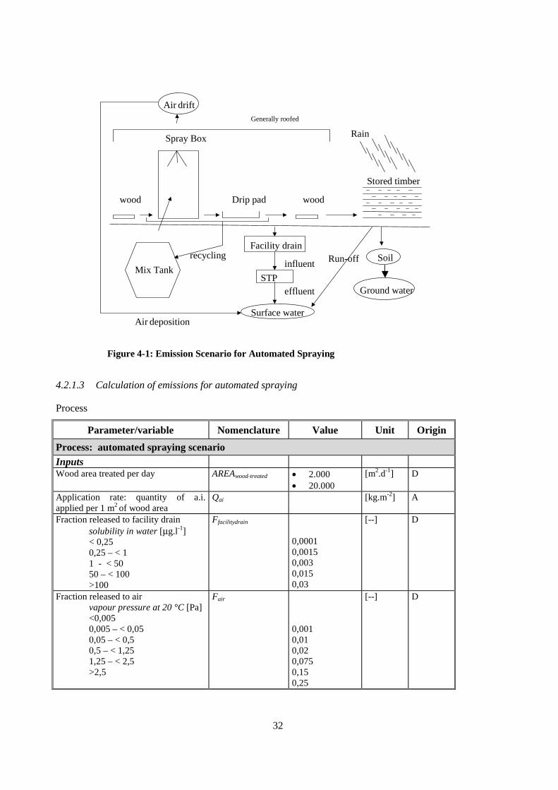
32

Figure 4-1: Emission Scenario for Automated Spraying

Facility drain

STP

influent

effluent

Run-offMix Tank

Spray Box

Drip padwood wood

Stored timber

Rain

recycling

Air driftGenerally roofed

Surface water

Soil

Ground water

Air deposition

4.2.1.3 Calculation of emissions for automated spraying

Process

Parameter/variable Nomenclature Value Unit Origin

Process: automated spraying scenario

Inputs Wood area treated per day AREAwood-treated • 2.000

• 20.000 [m2.d-1] D

Application rate: quantity of a.i. applied per 1 m2 of wood area

Qai [kg.m-2] A

Fraction released to facility drain solubility in water [µg.l-1] < 0,25 0,25 – < 1 1 - < 50 50 – < 100 >100

Ffacilitydrain 0,0001 0,0015 0,003 0,015 0,03

[--] D

Fraction released to air vapour pressure at 20 °C [Pa] <0,005 0,005 – < 0,05 0,05 – < 0,5 0,5 – < 1,25 1,25 – < 2,5 >2,5

Fair 0,001 0,01 0,02 0,075 0,15 0,25

[--] D

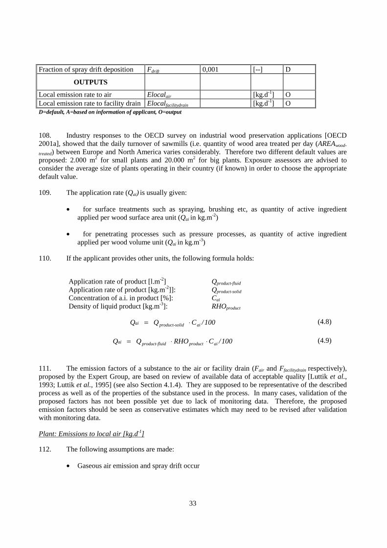
33

Fraction of spray drift deposition Fdrift 0,001 [--] D

OUTPUTS

Local emission rate to air Elocalair [kg.d-1] O Local emission rate to facility drain Elocalfacilitydrain [kg.d-1] O D=default, A=based on information of applicant, O=output

108. Industry responses to the OECD survey on industrial wood preservation applications [OECD 2001a], showed that the daily turnover of sawmills (i.e. quantity of wood area treated per day (AREAwood-

treated) between Europe and North America varies considerably. Therefore two different default values are proposed: 2.000 m2 for small plants and 20.000 m2 for big plants. Exposure assessors are advised to consider the average size of plants operating in their country (if known) in order to choose the appropriate default value.

109. The application rate (Qai) is usually given:

• for surface treatments such as spraying, brushing etc, as quantity of active ingredient applied per wood surface area unit (Qai in kg.m-2)

• for penetrating processes such as pressure processes, as quantity of active ingredient applied per wood volume unit (Qai in kg.m-3)

110. If the applicant provides other units, the following formula holds:

Application rate of product [l.m-2] Qproduct-fluid Application rate of product [kg.m-2]]: Qproduct-solid Concentration of a.i. in product [%]: Cai Density of liquid product [kg.m-3]: RHOproduct

100/C Q Q ailidproduct-soai ⋅= (4.8)

100/CRHO Q Q aiproductuidproduct-flai ⋅⋅= (4.9)

111. The emission factors of a substance to the air or facility drain (Fair and Ffacilitydrain respectively), proposed by the Expert Group, are based on review of available data of acceptable quality [Luttik et al., 1993; Luttik et al., 1995] (see also Section 4.1.4). They are supposed to be representative of the described process as well as of the properties of the substance used in the process. In many cases, validation of the proposed factors has not been possible yet due to lack of monitoring data. Therefore, the proposed emission factors should be seen as conservative estimates which may need to be revised after validation with monitoring data.

Plant: Emissions to local air [kg.d-1] 112. The following assumptions are made:

• Gaseous air emission and spray drift occur

34

Gaseous and spray air emissions deposit in the vicinity of the plant (within several 100 m). Emissions to local air can be calculated according to the following equation:

( )driftairaiedwood-treatair FFQ AREA Elocal +⋅⋅= (4.10)

Any point source emission model may be used to calculate soil deposition rates from air [mg.m-2.d-1] at 100m distance from the local source. Such a model is referenced in paragraph 274.

Plant: Emissions to facility drain [kg.d-1]

ainfacilitydraied wood-treatain facilitydr FQAREA Elocal ⋅⋅= (4.11)

Any sewage treatment plant model may be used to calculate surface water concentrations.

Storage

113. The calculation to determine emissions during storage is based on the proposed storage scenario outlined below, which includes the following assumptions:

• the storage area is uncovered and unpaved, therefore emissions may occur to soil and to surface water through leaching due to rainfall

• storage begins after post-treatment conditioning when the timber is placed on the storage area

• 3 rain events lasting ca. 60 min each every third day with a precipitation of 4mm.h-1 are considered to represent realistic worst-case for rainfall in many OECD countries (see also Section 4.1.5)

• per rain event, one half of the rainwater runs-off directly into the adjacent surface water body, the other half seeps into the storage soil. This assumption was agreed by the Expert Group as a compromise due to lack of data. The Expert Group was not aware of available data, where the fraction of rainwater which enters surface water or seeps into soil could be based on.

Parameter/variable Nomenclature Value Unit Origin

Storage: Spraying scenario

Inputs Effective surface area of treated wood, considered to be exposed to rain, per 1 m2 storage area (i.e. soil)

AREAwood-expo 11 [m2.m-2] D

Surface area of the storage place AREAstorage • 79 for plants with AREAwood-treated = 2.000 m2

• 790 for plants with AREAwood-treated = 20.000 m2

[m2] D

Duration of the initial assessment period

TIME1 30 [d] D

Duration of a longer assessment period TIME2 [d] D

35

Duration of storage of treated wood prior to shipment

TIMEstorage 3 [d] D

Average daily flux i.e. the average quantity of an active ingredient that is daily leached out of 1 m2 of treated wood during 3 day storage period [kg.m-2.d-1]

FLUXstorage,spray [kg.m-2.d-1] A

Volume of treated wood stacked per m2 of storage area (i.e. soil)

VOLUMEwood-stacked 2 [m3.m-2] D

Bulk density of wet soil RHOsoil 1700 [kg.m-3] D from TGD

Soil depth DEPTHsoil 0,1 [m] D Volume of (wet) soil Vsoil • 7,9 for plants with

AREAwood-treated =

2.000 m2

• 79 for plants with

AREAwood-treated =

20.000 m2

[m3] D

Fraction of rainwater running off the storage site

Frunoff 0,5 [-] D

OUTPUTS

Cumulative quantity of an active ingredient, leached due to rainfall from stored treated wood, over the initial assessment period

Qleach,storage,time1 [kg] O

Cumulative Quantity Of An Active Ingredient, Leached Due To Rainfall From Stored Treated Wood, Over A Longer Assessment Period

Qleach,storage,time2 [kg] O

Local Concentration In Soil At Storage Place At The End Of The Initial Assessment Period

Clocalsoil,time1 [kg.kgwwt-1] O

Local Concentration In Soil At Storage Place At The End Of A Longer Assessment Period

Clocalsoil,time2 [kg.kgwwt-1] O

Local Emission Rate In Surface Water Resulting From Leaching From Stored Treated Wood Due To Rain Run-Off, Over The Initial Assessment Period

Elocalsurfacewater,time1 [kg.d-1] O

Local Emission Rate In Surface Water Resulting From Leaching From Stored Treated Wood Due To Rain Run-Off, Over A Longer Assessment Period

Elocalsurfacewater,time2 [kg.d-1] O

D=default, A=based on information of applicant, O=output

36

Storage: Emissions at storage:

114. The emissions from a storage place, where treated wood is shipped out off site after a certain storage period (3 days are proposed for spray treatments by the Expert Group, based on industry responses to the OECD survey on industrial wood preservation applications [OECD 2001a]), are cumulative with time. Without taking into account removal processes, the cumulative quantity Qleach,storage of an active ingredient or any substance of concern in a wood preservative product leached (due to rainfall) from treated wood, can be calculated according to the generic equation 4.3 as follows:

• For an initial assessment period TIME1 (30 days are proposed by the Expert Group):

1TIME AREA AREA FLUX Q storageoexpwood-raystorage,sp1time,ageleach,stor ⋅⋅⋅= (4.12)

• For a longer assessment period TIME2:

2TIME AREA AREA FLUX Q storageoexpwood-raystorage,sp2age,timeleach,stor ⋅⋅⋅= (4.13)

• FLUXstorage,spray [kg.m-2.d-1]

115. The value of the average daily flux, FLUXstorage,spray, should be calculated based on the results of experimental leaching tests, in principle, with simulated rainfall. However, for the reasons explained in Section 4.1.5, it is acceptable for the initial assessment to use the results of a leaching test with wood in direct and continuous contact with water. The requirements for the design of such a leaching test are given in detail in Appendix 1.

116. Guidance on how the FLUXstorage,spray can be calculated from the results of the test is given in Appendix 2. It should be noted however, that the use of the average daily flux in equations 4.12 and 4.13 is a simplification and it can underestimate the amount of wood preservative lost in some cases. Further explanations on this issue are provided in Appendix 2.

• AREAwood-expo [m2.m-2]

117. The default value for the effective surface area of treated wood, exposed to rain per m2 storage area (i.e. soil), AREAwood-expo, is considered to be 11 [m2.m-2]. This default is derived as follows:

• based on the OECD survey on industrial wood preservation applications [OECD 2001a], the default value of 2 m3 stacked wood per m2 of soil (i.e. VOLUMEwood-stacked) is considered to represent a reasonable worst-case.

• the surface area of stacked wood exposed to and wetted by rain for a block of 2 m high and 1 m square is estimated as follows: 4 sides of 1 m by 2 m high, plus top and bottom of 1st layer (=2 m2), plus top of 2nd layer (1 m2) equals 11 m2.m-2 storage surface.

• AREAstorage [m2]

118. For processes such as spraying where the quantity of wood treated by the plant is given in area units, the wood volume (VOLUMEwood-treated) should be calculated in order to derive the storage area needed to accommodate the production during three days (i.e. the default storage duration), according to equation 4.4:

37

119. The VOLUMEwood-treated can be calculated as follows: according to the information provided by the American Chemistry Council (ACC) [Adrian Krygsman, pers. commun., 2001] the pieces of wood treated have a typical size of 105*105 mm.

• For a throughput (AREAwood-treated) of 2.000 m2 per day, the length of the rectangular will be 4760 m and its volume 52,5 m3.d-1.

• For a throughput (AREAwood-treated) of 20.000 m2 per day, the length of the rectangular will be 47600 m and its volume 525 m3.d-1.

120. The AREAstorage [m2] is then:

m792

5,523VOLUME

VOLUME TIME AREA 2

edwood-stack

edwood-treatstoragestorage =⋅⋅=⋅= small plants

m7902

5253 2=⋅= big plants

(4.14)

Storage: Local concentration in soil

121. It is assumed that one half of the rainwater runs-off directly into an adjacent surface water body, the other half seeps into the storage soil.

122. The concentration in local soil (Clocalsoil) over a given assessment period can be calculated as follows without taken into account removal processes. If removal processes are considered then (Clocalsoil) can be calculated as proposed in Section 7.1.1.

Storage: Concentration in soil at storage place at the end of the initial assessment period TIME1 (30 days are proposed by the Expert Group)[kg.kgwwt

-1]

soilsoil

1time,ageleach,storrunoff

soilsoil

1time,ageleach,stor 1time,soil RHOV

Q 2/1)F1(

RHOV

Q Clocal

⋅⋅=−

⋅=

(4.15)

Storage: Concentration in soil at storage place at the end of a longer assessment period TIME2 [kg.kgwwt

-1]

soilsoil

2time,ageleach,storrunoff

soilsoil

2time,ageleach,stor 2time,soil RHOV

Q 2/1)F1(

RHOV

Q Clocal

⋅⋅=−

⋅=

(4.16)

where:

Vsoil = (wet) soil volume [m3]

RHOsoil = (wet) soil bulk density [kg.m-3] 123. Emissions to soil may reach ground water. Some guidance on how to calculate these emissions using two models (i.e. PEARL and PELMO) is given in Appendix 4.

38

Storage: Emission rate to (adjacent) surface water

124. Surface water can receive run-off from storage sites. The releases to surface water from storage sites can be estimated as follows without taken into account removal processes. Section 7.2 (Chapter 7) proposes calculations when such processes are considered.

Storage: Emission rate from the storage place to an adjacent surface water body over an initial assessment period TIME1 (30 days are proposed by the Expert Group) [kg.d-1]

runoff1time,ageleach,stor

1time,ersurfacewat FTIME1

QElocal ⋅=

(4.17)

Storage: Emission rate from the storage place to an adjacent surface water body over a longer assessment period TIME2 [kg.d-1]

runoff2time,ageleach,stor

2time,ersurfacewat FTIME2

QElocal ⋅=

(4.18)

This release to surface water has to be added to the potential release to surface water from the treatment process.

For calculation of the local surface water concentration the following formula can be used:

ersurfacewat

ersurfacewatersurfacewat

ElocalClocal

FLOW=

FLOWsurfacewater is the flow rate of creek/river [m3s-1]

Elocalsurfacewater is the local surface water concentration[mg.L-1]

The OECD expert group did not give a default value for FLOWsurfacewater . This can be assumed to be a small creek with a flow rate of 0.3 m3s-1

4.2.2 Emission Scenario for Dipping/Immersion Processes

125. Dipping is considered to be a surface treatment and not a deep penetration treatment. Wood preservatives do not penetrate the wood more than three millimetres. We can distinguish two main types of industrial branches applying dipping/immersion for wood preservation purposes:

• Sawmills where freshly cut wood is treated with fungicides to prevent the discoloration caused by blue stain forming fungi. This treatment aims for a short-term preservation of wood until it is further processed.

ersurfacewatFLOW

ersurfacewatClocal

39

• Joinery industry and carpentry shops: ‘Joinery applications’ are industrial processes to treating wood articles that have been made to shape, for example fence panels, composites, window, doors and door frames, floors, architrave, decorative features. Carpentry shops fabricate wooden construction materials and treat them for long term protection against insects and fungi.

126. In some countries (such as Canada), the bases of utility poles (telephone and power transmission) are treated by dipping in an open vat operation with hot pentachlorophenol and/or creosote. The poles are left in the vat for several days to ensure penetration of the wood. Pole bottoms that are under soil are often perforated to increase preservative uptake in this area.

127. Despite small differences in the operation, dipping applied by the above three industrial sectors can be described by a generic ‘dipping/immersion scenario’.

4.2.2.1 Process description

128. Both automatic and manual dipping/immersion are batch processes. It involves submerging a pack or a single piece of wood into the dipping tank filled with a solution containing the preservative. Packs of wood are loaded on automatic equipment (e.g. hydraulic elevator) and lowered into a dipping tank. Wood remains there for a period usually between a few minutes and an hour (it is less than 30 seconds for sawmill anti-sapstain treatments but several days for the bases of utility poles). Cold soaking or steeping can extend over several days. Dipping baths can be heated in cold climate conditions. The treated wood is held over the dipping vat, usually for 30 minutes to an hour, in order the excess of the preservative solution to drain. Drips are usually collected and recycled into the process. Then the treated wood is removed to storage. Dipping facilities may be open or encapsulated, equipped with vapour trapping and air emission control.

4.2.2.2 Environmental Emission Pathways

129. The dipping baths are usually open and can lead to emissions to air by evaporation and co-distillation with water or the solvent. A distinction is made between wood preservative products dissolved in water and those using organic solvents as the carriers for the active substance. Organic solvents evaporate into the air.

130. In most countries such dipping facilities need to be authorised by government authorities according to environmental law or regulation. Recent regulations usually prescribe that dipping baths should be roofed and situated upon sealed flooring with no connection to the facility sewer system. Storm rainwater should be collected and be united with the tank impregnation solution. In addition, some industry associations have issued best practice guides for treating plants that provide instructions for environmental best practices including contamination of sites and surroundings (see Table 4-3). However, it should be borne in mind that open dipping facilities involve old technology and their operation may not fully comply with the requirements of recent regulations. Exposure assessors are advised to take national regulations into account.

131. Concerning the storage, a distinction is made between joineries and other facilities. Joineries in which the preservation treatment is applied on wooden articles that have been made to shape, (fence panels, composites, windows, doors and door frames, floors, architrave and decorative features) do not have an open storage area. These treated commodities/articles are immediately further processed (e.g. painted) and are not stored after wood preservation treatment.

40

132. The emission pathways identified for dipping plants are summarised in Table 4-5. Figure 4-2 schematically illustrates the dipping/immersion scenario.

TABLE 4.5 Emission Pathways At A Dipping/Immersion Plant

Primary medium Pathway Result Treatment process Local air • evaporations from open bath

• evaporations from hot/cold dipping • co-distillation with solvent • wind dispersal of dried salts • wind dispersal of saw dust

Elocalair

Facility drain pathways to the facility drain that subsequently drains to

the public sewage treatment plant (STP)

• water discharges of leaks at equipment, e.g. pumps, condensers, tank loading, on dilution

• cleaning water from the floor and equipment • drag-outs on tyres of vehicles • storm water overflow • cleaning of empty containers

Elocalfacilitydrain

Storage (only for sawmills and carpentry shops)* Local soil wood preservative components leaching due to rainfall;

rainwater seeping into soil when storage place is unpaved Clocalsoil

Adjacent surface water body

run-off water from unpaved storage into adjacent surface water body after rain event

Elocalsurfacewater

*In joineries the treated commodities/articles are immediately further processed (e.g. painted) and are not stored after wood preservation treatment.

41

Figure 4-2: Emission Scenario for Dipping/Immersion

(storage is not relevant for dipping processes at joineries)

Facility drain

STP

influent

effluent

SoilDip Tank

Drip padwood wood

Rain

recycling

Air

(mostly no roof)

Surface water

Ground water

Run-off

Stored timber

42

4.2.2.3 Calculation of emissions for dipping/immersion

Parameter/variable Nomenclature Value Unit Origin

Process: dipping/immersion scenario

Input Volume of wood treated per day VOLUMEwood-treated 100 [m3.d-1]* D

Application rate: quantity of a.i. applied per 1 m3 wood

Qai [kg.m-3] A

Fraction released to facility drain solubility in water [µg.l-1] < 0,25 0,25 – < 1 1 - < 50 50 – < 100 >100

Ffacilitydrain 0,0001 0,0015 0,003 0,015 0,03

[--] D

Fraction released to air vapour pressure at 20 °C [Pa] <0,005 0,005 – < 0,05 0,05 – < 0,5 0,5 – < 1,25 1,25 – < 2,5 >2,5

Fair 0,001 0,01 0,02 0,075 0,15 0,25

[--] D

OUTPUT EMISSIONS

Local emission rate to air Elocalair [kg.d-1] O Local emission rate to facility drain Elocalfacilitydrain [kg.d-1] O D=default, A=based on information of applicant, O=output

* In dipping/immersion applications the quantity of wood treated by the plant is expressed in m3 rather than m2, although dipping/immersion is considered to be a surface application.

Plant: Emission to local air [kg.d-1]

133. It is considered that the dipping bath is open to air and, therefore, evaporation of organic substances and water co-distillation can take place. Inorganic active ingredients do not emit to air. It is assumed that there are no ventilation or containment measures in place.

airaiedwood-treatair FQ VOLUME Elocal ⋅⋅= (4.19)

Plant: Emission to facility drain [kg.d-1]

ainfacilitydraiedwood-treatain facilitydr FQ VOLUME Elocal ⋅⋅= (4.20)

43

Storage

134. The storage scenario, proposed after treatment by spraying (see Section 4.2.1.3), is also valid for sawmills and carpentry shops applying dipping processes. As mentioned earlier, in joineries the treated commodities/articles are immediately further processed (e.g. painted) and are not stored after wood preservation treatment.

Parameter/variable Nomenclature Value Unit Origin

Storage: dipping scenario Inputs Effective surface area of treated wood, considered to be exposed to rain, per 1 m2 storage area (i.e. soil)

AREAwood-expo 11 [m2.m-2] D

Surface area of the storage place AREAstorage 700 [m2] D Duration of the initial assessment period TIME1 30 [d] D Duration of a longer assessment period TIME2 [d] D Duration of storage of treated wood prior to shipment

TIMEstorage 14 [d] D

Average daily flux i.e. the average quantity of an active ingredient that is daily leached out of 1 m2 of treated wood during 14 day storage period

FLUXstorage,dipp [kg.m-2.d-1] A

Volume of treated wood stacked per 1 m2 of storage area (i.e. soil)

VOLUMEwood-stacked 2 [m3.m-2] D

Bulk density of (wet) soil RHOsoil 1700 [kg.m-3] D from TGD Soil depth DEPTHsoil 0,1 [m] D Volume of (wet) soil Vsoil 70 [m3] D Fraction of rainwater running off the storage site

Frunoff 0,5 [-] D

Outputs

Cumulative quantity of an active ingredient, leached due to rainfall from stored treated wood over the initial assessment period

Qleach,storage,time1

[kg] O

Cumulative quantity of an active ingredient, leached due to rainfall from stored treated wood over a longer assessment period

Qleach,storage,time2

[kg] O

Local concentration in soil at storage place at the end of the initial assessment period

Clocalsoil,time1

[kg.kgwwt-1] O

Local concentration in soil at storage place at the end of a longer assessment period

Clocalsoil,time2

[kg.kgwwt-1] O

Local emission rate in surface water resulting from leaching from stored treated wood due to rain run-off, over the initial assessment period

Elocalsurfacewater,time1

[kg.d-1] O

Local emission rate in surface water resulting from leaching from stored treated wood due to rain run-off, over a longer assessment period

Elocalsurfacewater,time2

[kg.d-1] O

D=default, A=based on information of applicant, O=output

44

Storage: Emissions at storage:

135. The emissions from a storage place, where treated wood are shipped out off site after a certain storage period (14 days are proposed for dipping treatments by the Expert Group, based on industry responses to the OECD survey on industrial wood preservation applications [OECD 2001a], are cumulative with the time. Without taking into account removal processes, the cumulative quantity Qleach,storage of an active ingredient or any substance of concern in a wood preservative product leached (due to rainfall) from treated wood , can be calculated according to the generic equation 4.3 as follows:

• For an initial assessment period TIME1 (30 days are proposed by the Expert Group):

1TIME AREA AREA FLUX Q storageoexpwood-ppstorage,di1time,ageleach,stor ⋅⋅⋅= (4.21)

• For a longer assessment period TIME2:

2TIME AREA AREA FLUX Q storageoexpwood-ppstorage,di2time,ageleach,stor ⋅⋅⋅= (4.22)

• FLUXstorage,dipp [kg.m-2.d-1]

136. The value of the average daily flux, FLUXstorage,dipp, should be calculated based on the results of experimental leaching tests, in principle, with simulated rainfall. However, for the reasons explained in Section 4.1.5, it is acceptable for the initial assessment to use the results of a leaching test with wood in direct and continuous contact with water. The requirements for the design of such a leaching test are given in detail in Appendix 1.

137. Guidance on how the FLUXstorage,dipp can be calculated from the results of the leaching test is given in Appendix 2. It should be noted however that the use of the average daily flux in equations 4.21 and 4.22 is a simplification and it can underestimate the amount of wood preservative lost in some cases. Further explanations on this issue are provided in Appendix 2.

• AREAwood-expo [m2.m-2]

138. The default value for the effective surface area of treated wood, exposed to rain per m2 storage area (i.e. soil), AREAwood-expo, is considered to be 11 [m2.m-2]. This default is derived as follows:

• based on the OECD survey on industrial wood preservation applications [OECD 2001a], the default value of 2 m3 stacked wood per m2 of soil (i.e. VOLUMEwood-stacked) is considered to represent a reasonable worst-case.

• the surface area of stacked wood exposed to and wetted by rain for a block of 2 m high and 1 m square is estimated as follows: 4 sides of 1 m by 2 m high, plus top and bottom of 1st layer (=2 m2), plus top of 2nd layer (1 m2) equals 11 m2.m-2 storage surface.

• AREAstorage [m2]:

139. For processes where the quantity of treated wood is given in volume units, the storage area is calculated according to equation 4.4 and the default values proposed for the dipping scenario:

45

m700210014

VOLUME VOLUME TIMEAREA 2

edwood-stack

edwood-treatstoragestorage =⋅=⋅= (4.23)

Storage: Local concentration in soil

140. It is assumed that one half of the rainwater runs-off directly into an adjacent surface water body, the other half seeps into the storage soil.

141. The concentration in local soil (Clocalsoil) over a given assessment period can be calculated as follows without taken into account removal processes. If removal processes are considered then (Clocalsoil) can be calculated as proposed in Section 7.1.1.

Storage: Concentration in soil at storage place at the end of the initial assessment period TIME1 (30 days are proposed by the Expert Group) [kg.kgwwt

-1]

soilsoil

1time,ageleach,stor)runoff

soilsoil

1time,ageleach,stor 1time,soil RHOV

Q 2/1F1(

RHOV

Q Clocal

⋅⋅

=−⋅⋅

= (4.24)

Storage: Concentration in soil at storage place at the end of a longer assessment period TIME2 [kg.kgwwt

-1]

soilsoil

2time,ageleach,stor)runoff

soilsoil

2time,ageleach,stor 2time,soil RHOV

Q 2/1F1(

RHOV

Q Clocal

⋅⋅=−⋅

⋅=

(4.25)

where:

Vsoil = (wet) soil volume [m3]

RHOsoil = (wet) soil bulk density [kg.m-3] 142. Emissions to soil may reach ground water. Some guidance on how to calculate these emissions using two models (i.e. PEARL and PELMO) is given in Appendix 4.

Storage: Emission rate to (adjacent) surface water

143. Surface water can receive run-off from storage sites. The releases to surface water from storage sites can be estimated as follows without taken into account removal processes. Section 7.2 (Chapter 7) proposes calculations when such processes are considered.

Storage: Emission rate from the storage place to an adjacent surface water body over an initial assessment period TIME1 (30 days are proposed by the Expert Group) [kg.d-1]

runoff1time,ageleach,stor

1time,ersurfacewat FTIME1

QElocal ⋅=

(4.26)

Storage: Emission rate from the storage place to an adjacent surface water body over a longer assessment period TIME2 [kg.d-1]

46

runoff2time,ageleach,stor

2time,ersurfacewat FTIME2

QElocal ⋅=

(4.27)

This release to surface water has to be added to the potential release to surface water from the treatment process.

4.2.3 Emission Scenario for Vacuum-Pressure and Double-Vacuum/Low Pressure Processes

144. Pressure processes are techniques used to apply wood preservative by overcoming the resistance of the wood to deep penetration using pressure. The treatment is carried out in cylindrical airtight steel pressure/vacuum vessels. Two general categories of processes can be distinguished:

• the pressure-vacuum process: vacuum – flood with preservation liquid – pressure applied (range between 800 and 1400 kPa) – pressure released, pump off liquid. 250 – 500 l.m-3 preservative solution is normally used.

• the double-vacuum/low pressure process: vacuum – flood with preservation liquid – low pressure applied (up to 200 kPa) – pump off liquid – end vacuum. 20 – 400 l.m-3 preservative solution is normally used.

Both processes are handled in one emission scenario, because the emission pathways are similar.

4.2.3.1 Process description

145. Generally, the pressure processes includes the following steps:

1. Untreated wood is loaded onto small rails or trams cars (bogies) that are pushed into the cylinder using forklifts or other mechanical means.

2. The cylinder door is sealed via a pressure tight door, either manually with bolts or hydraulically, and a vacuum applied to remove most of the air from the cylinder and the wood cells.

3. Treating solutions (either heated or at ambient temperature depending on the system) are then pumped into the cylinder and the pressure raised. The total treating time and cycles will vary, depending on the species of wood, the commodity being treated, and the desired product retention, but in all instances the treating process remains a closed system.

4. At the end of the pressure period, the pressure is released and the excess solution is removed from the cylinder, typically by pumping and goes back to the storage for re-use.

5. A final vacuum may be applied to remove the excess preservative that would otherwise drip from the wood. This final vacuum may recover 20-60 percent of the gross amount of the preservative injected.

6. The final steps in the process are the unloading of the retort and storage of the treated wood.

47

The preservative is usually delivered to the plant in the form of a concentrate and must be diluted down to a suitable working strength. The degree of dilution will vary depending on the wood species, type of wood product, and anticipated use.

Wood preservatives

146. Whilst it has been the custom and tradition to categorise industrial wood preservatives applied by vacuum pressure or double vacuum/low pressure processes into waterborne and oilborne preservatives these categories are less relevant in today’s industry with the very wide range of active substances used and the formulating technologies used.

147. Section 2.2 describes the principle formulation types used in vacuum pressure and double vacuum pressure/low pressure processes. The selection of the preservative type used for a particular application will depend on:

• the end use for the treated timber

• the biological hazard the timber may be exposed to

• the desired service life

• the ancillary properties of the treated timber e.g. painting

148. Creosote contains carcinogenic polyaromatic hydrocarbons (PAHs) with benzo[a]pyrene as the lead substance. , Creosote and tar oils can result in VOC emissions that need to be reduced [EU Directive 99/13/EC of 11 March 1999]. EU Member countries are engaged to minimise the risk from creosote based wood preservatives by promoting low volatile and low benzo[a]pyren fractions of creosote. In Denmark, creosote l is not approved for domestic wood preservation but is allowed in imported wood; In the US creosote and coal tar distillate based products have been used in the past for wood treatment but they are no longer in use.

TABLE 4.6 Classification of Impregnating Oils (Creosote) according to the WEI (Status: October 1994)

Technical data Unit Method of estimation

WEI Grade A

WEI Grade B

WEI Grade C

Density (20 °C) g ml-1 WEI App.3 1,04-1,15 1,02-1,15 1,03-1,17

Water content Vol % WEI App.4 max. 1 max. 1 max. 1

Crystallisation temperature °C WEI App.5 max. 23 max. 23 max. 50

Water-extract. phenols Weight % EN 1014-4 max. 3 max. 3 max. 3

Insoluble matter Weight % BS 144

App. J

max. 0.4 max. 0.4 max. 0.4

Boiling range

- distillate to 235 °C - distillate to 300 °C - distillate to 355 °C

vol %

WEI App. 8

max. 10 20-40 55-75

max. 20 40-60 70-90

--- max. 10 65-95

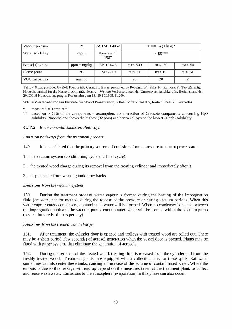
48

Vapour pressure Pa ASTM D 4052 < 100 Pa (1 hPa)*

Water solubility mg/L Raven et al. 1987

∑ 90***

Benzo[a]pyrene ppm = mg/kg EN 1014-3 max. 500 max. 50 max. 50

Flame point °C ISO 2719 min. 61 min. 61 min. 61

VOC emissions max % 25 20 2

Table 4-6 was provided by Rolf Peek, BHF, Germany. It was presented by Boenigk, W.; Behr, H.; Komora, F.: Teerstämmige Holzschutzmittel für die Kesseldruckimprägnierung – Weitere Verbesserungen der Umweltverträglichkeit. In: Berichtsband der 20. DGfH Holzschutztagung in Rosenheim vom 18.-19.10.1995, S. 200.

WEI = Western-European Institute for Wood Preservation, Allée Hofter-Vleest 5, bôite 4, B-1070 Bruxelles

* measured at Temp 20°C ** based on ~ 60% of the components – assumption: no interaction of Creosote components concerning H2O

solubility. Naphthalene shows the highest (32 ppm) and benzo-(a)-pyrene the lowest (4 ppb) solubility.

4.2.3.2 Environmental Emission Pathways

Emission pathways from the treatment process

149. It is considered that the primary sources of emissions from a pressure treatment process are:

1. the vacuum system (conditioning cycle and final cycle).

2. the treated wood charge during its removal from the treating cylinder and immediately after it.

3. displaced air from working tank blow backs

Emissions from the vacuum system

150. During the treatment process, water vapour is formed during the heating of the impregnation fluid (creosote, not for metals), during the release of the pressure or during vacuum periods. When this water vapour enters condensers, contaminated water will be formed. When no condenser is placed between the impregnation tank and the vacuum pump, contaminated water will be formed within the vacuum pump (several hundreds of litres per day).

Emissions from the treated wood charge

151. After treatment, the cylinder door is opened and trolleys with treated wood are rolled out. There may be a short period (few seconds) of aerosol generation when the vessel door is opened. Plants may be fitted with purge systems that eliminate the generation of aerosols.

152. During the removal of the treated wood, treating fluid is released from the cylinder and from the freshly treated wood. Treatment plants are equipped with a collection tank for these spills. Rainwater sometimes can also enter these tanks, causing an increase of the volume of contaminated water. Where the emissions due to this leakage will end up depend on the measures taken at the treatment plant, to collect and reuse wastewater. Emissions to the atmosphere (evaporation) in this phase can also occur.

49

153. Assuming that the impregnation plant is fitted with collectors to remove water vapour from the air, the main emissions will be directed to a public sewage treatment plant (STP) or to surface water. Depending on the configuration of the plant, spilled impregnation fluid will be emitted to:

• the air (outdoors)

• soil or surface water (when the area of the plant is not paved)

• a public STP or surface water (when the area is paved).

Emissions due to working tank blow backs

154. Working tank blow backs also occur at the end of a preservative treatment cycle when the treating solution is returned to the work tank. The air displaced by the returning solution is vented via a control device to the atmosphere. In some systems, the displaced air in the work tank is vented back into the treatment cylinder to fill the head space created as the preservative is withdrawn from the cylinder. In such systems, there are no emissions associated with blow backs. A problem may arise when the quantity of the preservative being blown back is not monitored closely and air begins to blow up through the work tank. Volatile compounds are picked up by the air as it bubbles up through the treating solution and carried out through the tank vent.

Other emission sources for plants using creosote preservatives

155. In addition to the three primary process emission sources, emissions are generated from wastewater treatment and organic liquid storage tanks. Creosote wood treatment plants frequently have on-site wastewater treatment facilities designed to separate organic materials from the wastewater generated during the treating process. This is a potential source of VOC and HAP. Liquid storage tanks for the various preservatives are also sources of VOC and HAP. Emissions from these sources are not covered in this document.

Emissions pathways from storage

156. It is considered that storage does not take place after double-vacuum treatments at joineries. The reason for this is that such treatments/processes are normally applied on wood articles that have been made to shape, for example fence panels, composites, windows, doors and door frames, floors, architrave and decorative features. These treated commodities/articles are immediately further processed (e.g. painted) and therefore they are not stored after wood preservation treatment.

Therefore, the storage scenario considered here is only relevant for vacuum-pressure treatments in the case that storage area is unpaved and uncovered.

Overview of the environmental emission pathways

157. Table 4-7 provides an overview of the emission pathways for the pressure processes. Figure 4-3 schematically illustrates the scenario for pressure-vacuum. Exposure assessors are advised however to take national regulations into account because some emission pathways and compartments exposed, proposed in this document, may not apply for their country (see also Section 4.1.3)

50

TABLE 4.7

Environmental Emission Pathways for the vacuum-pressure and double vacuum processes

Primary medium Pathway Result Treatment process Local air • cease of vacuum: removal of surplus and residual amounts

of organic solvent or creosote, • boiling the creosote • aerosol air drifts • removal of the wood from the impregnation tank (main

release), evaporation losses of solvents can be up to 20% • fugative diffusive emissions from equipment • wind dispersal of dried salts or saw dust

Elocalair

Facility drain pathways to the facility drain that subsequently drains to the public sewage treatment plant (STP): • water discharge of leaks at equipment (e.g. pumps,

condensers, tank loading, on dilution) • cleaning water from the floor, the equipment, and drip pad • drag-outs on tyres of vehicles • washing disposals to facility sewer • contaminated rain water out flows • cleaning of empty preservative containers • losses at fixation

Elocalfacilitydrain

Storage Local soil wood preservative components leaching due to rainfall; rainwater

seeping into soil when storage place is unpaved Clocalsoil

Adjacent surface water run-off water from unpaved storage into adjacent surface water body after rainfall

Elocalsurfacewater

Facility drain

STP

influent

effluent

Mix Tank

Pressure Vessel

Drip padWood Wood

Rain

recycling

Air

roof

Surface water

Soil

Stored timber

Groundwater

Figure 4-3: Emission Scenario for vacuum-pressure & double-vacuum/low pressure processes (storage is

not relevant for double-vacuum processes at joineries)

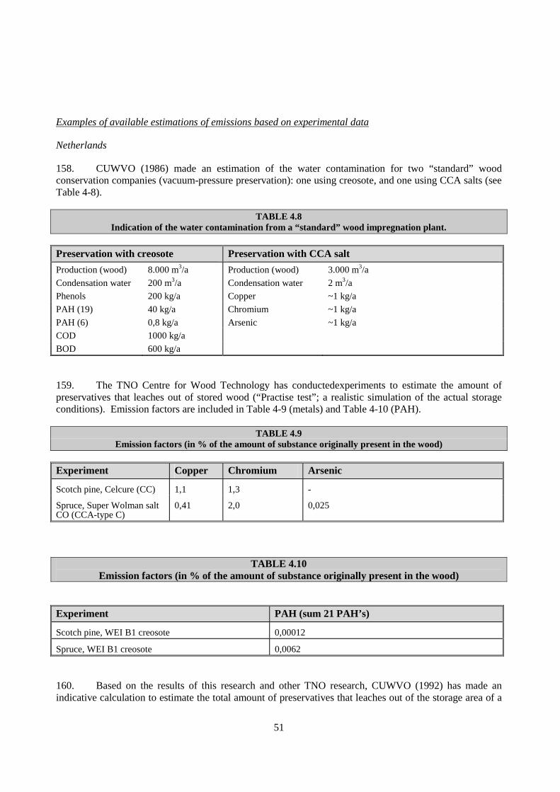
51

Examples of available estimations of emissions based on experimental data

Netherlands

158. CUWVO (1986) made an estimation of the water contamination for two “standard” wood conservation companies (vacuum-pressure preservation): one using creosote, and one using CCA salts (see Table 4-8).

TABLE 4.8 Indication of the water contamination from a “standard” wood impregnation plant.

Preservation with creosote Preservation with CCA salt

Production (wood) 8.000 m3/a Production (wood) 3.000 m3/a

Condensation water 200 m3/a Condensation water 2 m3/a

Phenols 200 kg/a Copper ~1 kg/a

PAH (19) 40 kg/a Chromium ~1 kg/a

PAH (6) 0,8 kg/a Arsenic ~1 kg/a

COD 1000 kg/a

BOD 600 kg/a

159. The TNO Centre for Wood Technology has conductedexperiments to estimate the amount of preservatives that leaches out of stored wood (“Practise test”; a realistic simulation of the actual storage conditions). Emission factors are included in Table 4-9 (metals) and Table 4-10 (PAH).

TABLE 4.9 Emission factors (in % of the amount of substance originally present in the wood)

Experiment Copper Chromium Arsenic

Scotch pine, Celcure (CC) 1,1 1,3 -

Spruce, Super Wolman salt CO (CCA-type C)

0,41 2,0 0,025

TABLE 4.10 Emission factors (in % of the amount of substance originally present in the wood)

Experiment PAH (sum 21 PAH’s)

Scotch pine, WEI B1 creosote 0,00012

Spruce, WEI B1 creosote 0,0062

160. Based on the results of this research and other TNO research, CUWVO (1992) has made an indicative calculation to estimate the total amount of preservatives that leaches out of the storage area of a

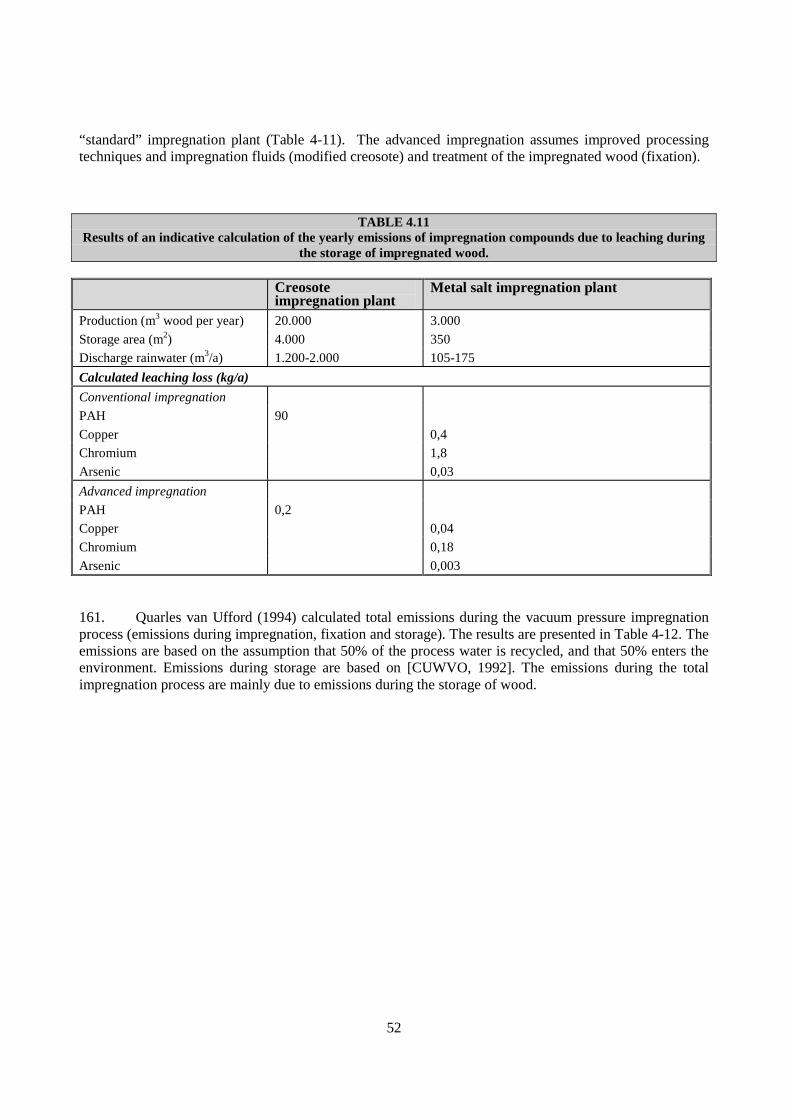
52

“standard” impregnation plant (Table 4-11). The advanced impregnation assumes improved processing techniques and impregnation fluids (modified creosote) and treatment of the impregnated wood (fixation).

TABLE 4.11 Results of an indicative calculation of the yearly emissions of impregnation compounds due to leaching during

the storage of impregnated wood.

Creosote impregnation plant

Metal salt impregnation plant

Production (m3 wood per year) 20.000 3.000

Storage area (m2) 4.000 350

Discharge rainwater (m3/a) 1.200-2.000 105-175

Calculated leaching loss (kg/a)

Conventional impregnation

PAH 90

Copper 0,4

Chromium 1,8

Arsenic 0,03

Advanced impregnation

PAH 0,2

Copper 0,04

Chromium 0,18

Arsenic 0,003

161. Quarles van Ufford (1994) calculated total emissions during the vacuum pressure impregnation process (emissions during impregnation, fixation and storage). The results are presented in Table 4-12. The emissions are based on the assumption that 50% of the process water is recycled, and that 50% enters the environment. Emissions during storage are based on [CUWVO, 1992]. The emissions during the total impregnation process are mainly due to emissions during the storage of wood.

53

TABLE 4.12 Emissions during impregnation with the vacuum-pressure method (impregnation, fixation, storage)

Substance Average input

(kg.m-3 wood)

Air

(kg.m-3 wood)

(Process) water

(mg.m-3 wood)

Leaching during storage: Range

(mg.m-3 wood)

Leaching during storage: 1990

(mg.m-3 wood)

total VOC 20 7 Naphthalene 8 3 ? 300 Fenanthrene 8 0,8 ? 3-1.000 150 Fluoranthene 4 0,125 50 3-1.000 150 Benzo(a)pyrene 0,02 0 <1 1,4 21 PAH 20 (?) >1 ? 10-4.500 700 Copper 0,6 0 0 13-130 100 Chromium 1 0 0 60-600 450 Arsenic 0.8 0 0 1-10 8 Zinc 0 0 p.m. Fluoride 0 0 p.m.

USA

162. US EPA has reviewed available data in plants using creosote and CCA in order to propose emission factors for the AP-42 ‘Compilation of Air Pollutant Emission Factors’, Section 10.8, Wood Preserving [EPA 1999]. Table 4-13 summarises:

1) the test data for VOC releases from the vacuum system during conditioning (boulton) cycle in an empty-cell creosote wood preserving and

2) the estimated emission factors from the whole process which includes emissions from the conditioning by boulton process + preservative filling/air release + preservative return/blowback + vacuum.

TABLE 4-13 Summary of test data on emissions to the air from empty-cell creosote wood impregnation process

Emission factors in lb.ft-3 of wood treated [Conversion factor: 1 kg.m-3 = 16 lb.ft-3]

Conditioning by Boulton process (test data)

Total, with

conditioning by

Boulton processa

(estimates based on test data)

Total, without conditioning (estimates based on test data)

Substance

lb.ft-3 kg.m-3 lb.ft-3 kg.m-3 lb.ft-3 kg.m-3 VOC 5,10E-03 8.16E-02 5,80E-03 9,28E-02 7,40E-04 1,18E-02 Acenaphthene 9,30E-06 1,49E-04 9,90E-06 1,58E-04 6,30E-07 1,01E-05 Acenaphthylene 2,60E-05 4,16E-04 2,80E-05 4,48E-04 1,70E-07 2,72E-06 Anthracene 1,10E-07 1,76E-06 1,30E-07 2,08E-06 1,60E-08 2,56E-07

54

Benzo(a)anthracene 1,20E-07 1,92E-06 1,30E-07 2,08E-06 1,70E-08 2,72E-07 Benzo(b)flouranthene 1,10E-07 1,76E-06 1,30E-07 2,08E-06 1,60E-08 2,56E-07 Benzo(k)flouranthene 4,20E-07 6,72E-06 4,80E-08 7,68E-07 6,00E-09 9,60E-08 Benzo(a)pyrene 5,60E-08 8,96E-07 6,50E-08 1,04E-06 8,20E-09 1,31E-07 Carbazole 2,50E-06 4,00E-05 2,90E-06 4,64E-05 3,60E-07 5,76E-06 Chrysene 5,90E-08 9,44E-07 6,70E-08 1,07E-06 8,40E-06 1,34E-04 Dibenzofuran 3,30E-05 5,28E-04 3,50E-05 5,60E-04 1,80E-06 2,88E-05 Fluoranthene 5,90E-07 9,44E-06 6,80E-07 1,09E-05 8,60E-08 1,38E-06 Fluorene 3,80E-06 6,08E-05 3,90E-06 6,24E-05 7,80E-08 1,25E-06 Naphthalene 7,40E-05 1,18E-03 7,90E-05 1,26E-03 4,60E-06 7,36E-05 Phenanthrene 1,60E-06 2,56E-05 1,90E-06 3,04E-05 2,80E-07 4.48E-06 Pyrene 5,10E-07 8,16E-06 5,80E-07 9,28E-06 7,30E-08 1.17E-06 aDoes not include emissions from preservative return/blowback associated with Boulton process

163. Table 4-14 summarises test data for emissions from the vacuum system/cycle during empty-cell CCA impregnation.

Table 4.14 Summary of test data on emissions to the air from the vacuum system/cycle during empty-cell CCA

impregnation [from US EPA 1999 & Australia 1999]

Substance CASRNa Emission factor

Data ratingb

average in kg. m-3

(kg of pollutant per 1m3 of wood treated)

average in lb. ft-3

(lb of pollutant per 1ft3 of wood treated)

Arsenicc 2,20E-08 1,40E-09 D

Chromiumd 7440-47-3 2,20E-08 1,40E-09 D

Copper 7440-50-8 3,00E-08 1,90E-09 D

a. CASRN: Chemical Abstracts Service Registry Number.

b. D means tests that were based on generally unacceptable method but may provided an order-of-magnitude value for the source.

c. Source of arsenic emission factor: Timber Preservers Association of Australia, 1999.

d. it can reasonably be assumed that all the chromium is present as chromium VI.

Canada

164. Environment Canada made a study to evaluate the leachability characteristics of CCA from stored wood products and their potential contribution to stormwater discharges. The results of this study are summarised in Table 4-15.

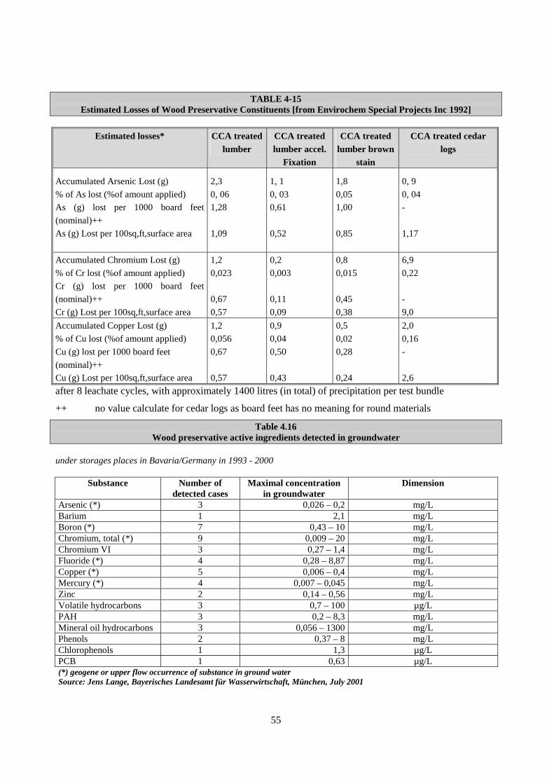
55

TABLE 4-15 Estimated Losses of Wood Preservative Constituents [from Envirochem Special Projects Inc 1992]

Estimated losses* CCA treated lumber

CCA treated lumber accel.

Fixation

CCA treated lumber brown

stain

CCA treated cedar logs

Accumulated Arsenic Lost (g) 2,3 1, 1 1,8 0, 9

% of As lost (%of amount applied) 0, 06 0, 03 0,05 0, 04

As (g) lost per 1000 board feet

(nominal)++

1,28 0,61 1,00 -

As (g) Lost per 100sq,ft,surface area 1,09 0,52 0,85 1,17

Accumulated Chromium Lost (g) 1,2 0,2 0,8 6,9

% of Cr lost (%of amount applied) 0,023 0,003 0,015 0,22

Cr (g) lost per 1000 board feet

(nominal)++ 0,67 0,11 0,45 -

Cr (g) Lost per 100sq,ft,surface area 0,57 0,09 0,38 9,0

Accumulated Copper Lost (g) 1,2 0,9 0,5 2,0

% of Cu lost (%of amount applied) 0,056 0,04 0,02 0,16

Cu (g) lost per 1000 board feet

(nominal)++

0,67 0,50 0,28 -

Cu (g) Lost per 100sq,ft,surface area 0,57 0,43 0,24 2,6

after 8 leachate cycles, with approximately 1400 litres (in total) of precipitation per test bundle

++ no value calculate for cedar logs as board feet has no meaning for round materials

Table 4.16 Wood preservative active ingredients detected in groundwater

under storages places in Bavaria/Germany in 1993 - 2000

Substance Number of detected cases

Maximal concentration in groundwater

Dimension

Arsenic (*) 3 0,026 – 0,2 mg/L Barium 1 2,1 mg/L Boron (*) 7 0,43 – 10 mg/L Chromium, total (*) 9 0,009 – 20 mg/L Chromium VI 3 0,27 – 1,4 mg/L Fluoride (*) 4 0,28 – 8,87 mg/L Copper (*) 5 0,006 – 0,4 mg/L Mercury (*) 4 0,007 – 0,045 mg/L Zinc 2 0,14 – 0,56 mg/L Volatile hydrocarbons 3 0,7 – 100 µg/L PAH 3 0,2 – 8,3 mg/L Mineral oil hydrocarbons 3 0,056 – 1300 mg/L Phenols 2 0,37 – 8 mg/L Chlorophenols 1 1,3 µg/L PCB 1 0,63 µg/L (*) geogene or upper flow occurrence of substance in ground water Source: Jens Lange, Bayerisches Landesamt für Wasserwirtschaft, München, July 2001

56

4.2.3.3 Calculation of emissions for Vacuum-Pressure and Double-Vacuum/Low Pressure Treatment

Process

Parameter/variable Nomenclature Value Unit Origin

Process: Vacuum-pressure & double vacuum-low pressure

Inputs

Volume of wood treated per day • vacuum-pressure • double vacuum

VOLUMEwood-treated • 30 • 15

[m3.d-1] D

Application rate: Quantity of a.i. applied per m3 wood

Qai [kg.m-3] A

Fraction released to facility drain solubility in water [µg.l-1] < 0,25 0,25 – < 1 1- < 50 50 – < 100 >100

Ffacilitydrain 0,0001 0,0015 0,003 0,015 0,03

[--] D

Fraction released to air vapour pressure at 20 °C [Pa] <0,005 0,005 – < 0,05 0,05 – < 0,5 0,5 – < 1,25 1,25 – < 2,5 >2,5

Fair 0,001 0,01 0,02 0,075 0,15 0,25

[--] D

Outputs

Local emission rate to air Elocalair [kg.d-1] O Local emission rate to facility drain Elocalfacilitydrain [kg.d-1] O D=default, A=based on information of applicant, O=output

Plant: Emission to local air

airaiedwood-treatair FQ VOLUME Elocal ⋅⋅= (4.28)

Plant: Emission to facility drain

ainfacilitydraiedwood-treatain facilitydr FQ VOLUME Elocal ⋅⋅= (4.29)

57

Storage

The proposed scenario is not relevant for double-vacuum/low pressure processes at joineries.

Parameter/variable Nomenclature Value Unit Origin

Storage: Vacuum pressure scenario Input Effective surface area of treated wood, considered to be exposed to rain, per m2 storage area (i,e, soil)

AREAwood-expo 11 [m2.m-2] D

Surface area of the storage place AREAstorage • 525 for vac-pres plants with VOLUMEwood-treated = 30 m3

• 263 for double vac plants with VOLUMEwood-treated = 15 m3

[m2] D

Duration of the initial assessment period

TIME1 30 [d] D

Duration of a longer term assessment period

TIME2 [d] D

Duration of storage of treated wood prior to shipment

TIMEstorage 35 [d] D

Average daily flux ie the average quantity of an active ingredient that is daily leached out of 1 m2 of treated wood during 35 day storage period

FLUXstorage,vac-pres [kg.m-2.d-1] A

Volume of treated wood stacked per 1 m2 of storage area (i.e. soil)

VOLUMEwood-stacked 2 [m3.m-2] D

Bulk density of wet soil RHOsoil 1700 [kg.m-3] TGD Soil depth DEPTHsoil 01 [m] D Volume of wet soil Vsoil • 52,5 for vac-pres

plants

• 26,3 for double vac plants

[m3] D

Fraction of rainwater running off the storage site

Frunoff 0,5 [-] D

Output Cumulative quantity of an active ingredient, leached due to rainfall from stored treated wood over the initial assessment period

Qleach,storage,time1 [kg] O

Cumulative quantity of an active ingredient, leached due to rainfall from stored treated wood over a longer assessment period

Qleach,storage,,time2 [kg] O

Local concentration in soil at storage place at the end of the initial assessment period

Clocalsoil,time1 [kg.kgwwt-1] O

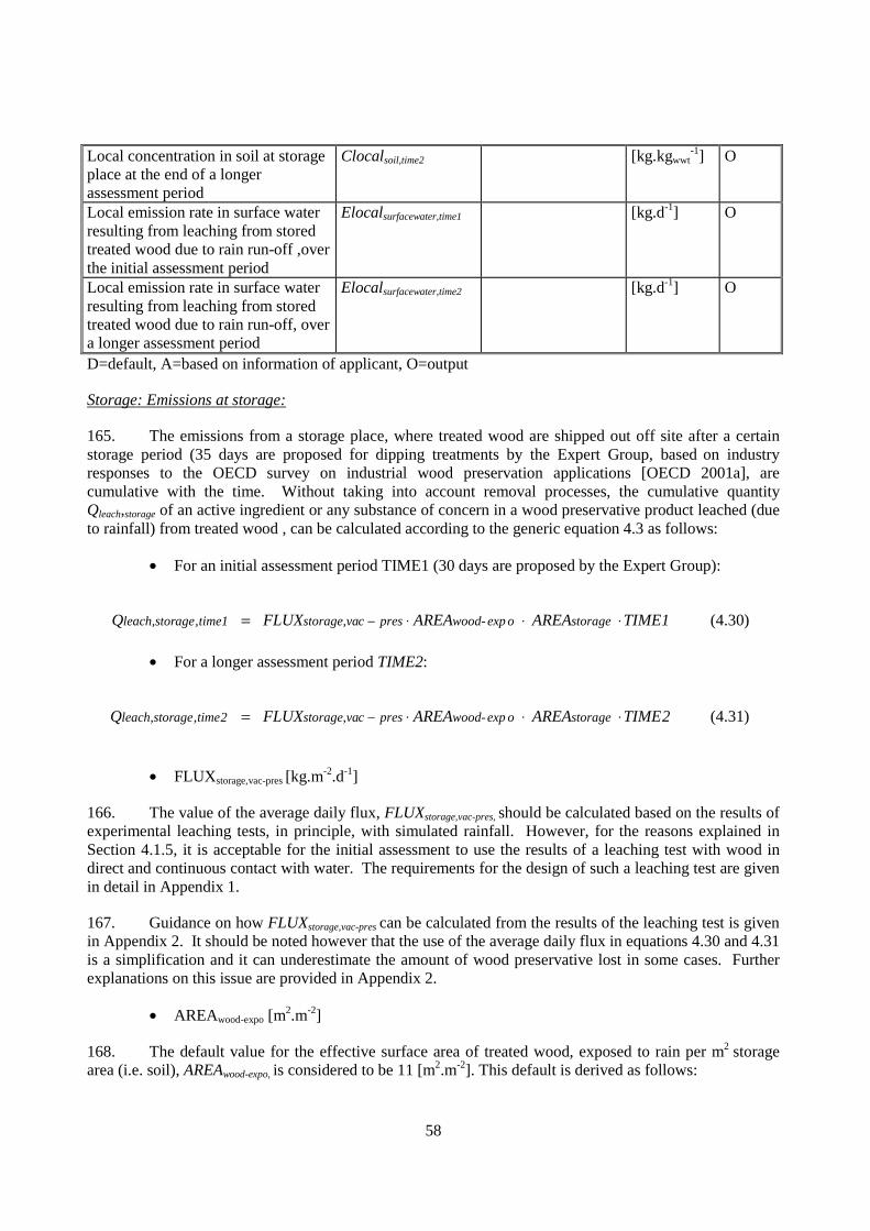
58

Local concentration in soil at storage place at the end of a longer assessment period

Clocalsoil,time2 [kg.kgwwt-1] O

Local emission rate in surface water resulting from leaching from stored treated wood due to rain run-off ,over the initial assessment period

Elocalsurfacewater,time1 [kg.d-1] O

Local emission rate in surface water resulting from leaching from stored treated wood due to rain run-off, over a longer assessment period

Elocalsurfacewater,time2 [kg.d-1] O

D=default, A=based on information of applicant, O=output

Storage: Emissions at storage:

165. The emissions from a storage place, where treated wood are shipped out off site after a certain storage period (35 days are proposed for dipping treatments by the Expert Group, based on industry responses to the OECD survey on industrial wood preservation applications [OECD 2001a], are cumulative with the time. Without taking into account removal processes, the cumulative quantity Qleach,storage of an active ingredient or any substance of concern in a wood preservative product leached (due to rainfall) from treated wood , can be calculated according to the generic equation 4.3 as follows:

• For an initial assessment period TIME1 (30 days are proposed by the Expert Group):

1TIME AREA AREA FLUX Q storageoexpwood-prescstorage,va1time,ageleach,stor ⋅⋅⋅= − (4.30)

• For a longer assessment period TIME2:

2TIME AREA AREA FLUX Q storageoexpwood-prescstorage,va2time,ageleach,stor ⋅⋅⋅= − (4.31)

• FLUXstorage,vac-pres [kg.m-2.d-1]

166. The value of the average daily flux, FLUXstorage,vac-pres, should be calculated based on the results of experimental leaching tests, in principle, with simulated rainfall. However, for the reasons explained in Section 4.1.5, it is acceptable for the initial assessment to use the results of a leaching test with wood in direct and continuous contact with water. The requirements for the design of such a leaching test are given in detail in Appendix 1.

167. Guidance on how FLUXstorage,vac-pres can be calculated from the results of the leaching test is given in Appendix 2. It should be noted however that the use of the average daily flux in equations 4.30 and 4.31 is a simplification and it can underestimate the amount of wood preservative lost in some cases. Further explanations on this issue are provided in Appendix 2.

• AREAwood-expo [m2.m-2]

168. The default value for the effective surface area of treated wood, exposed to rain per m2 storage area (i.e. soil), AREAwood-expo, is considered to be 11 [m2.m-2]. This default is derived as follows:

59

• based on the OECD survey on industrial wood preservation applications [OECD 2001a], the default value of 2 m3 stacked wood per m2 of soil (i.e. VOLUMEwood-stacked) is considered to represent a reasonable worst-case.

• the surface area of stacked wood exposed to and wetted by rain for a block of 2 m high and 1 m square is estimated as follows: 4 sides of 1 m by 2 m high, plus top and bottom of 1st layer (=2 m2), plus top of 2nd layer (1 m2) equals 11 m2.m-2 storage surface.

• AREAstorage [m2]:

169. For processes where the quantity of treated wood is given in volume units, the storage area is calculated according to equation 4.4 and the default values proposed for the vacuum-pressure scenario:

pressurevacuumform52523035

VOLUME VOLUME TIMEAREA 2

edwood-stack

edwood-treatstoragestorage −=⋅=⋅=

(4.32)

vacuumdoubleform26321535 2=⋅=

Storage: Local concentration in soil

170. It is assumed that one half of the rainwater runs-off directly into an adjacent surface water body, the other half seeps into the storage soil.

171. The concentration in local soil (Clocalsoil) over a given assessment period can be calculated as follows without taken into account removal processes. If removal processes are considered then (Clocalsoil) can be calculated as proposed in Section 7.1.1.

Storage: Concentration in soil at storage place at the end of the initial assessment period TIME1 (30 days are proposed by the Expert Group) [kg.kgwwt

-1]

soilsoil

1time,ageleach,storrunoff

soilsoil

1time,ageleach,stor 1time,soil RHOV

Q 2/1)F1(

RHOV

Q Clocal

⋅⋅=−⋅

⋅=

(4.33)

Storage: Concentration in soil at storage place at the end of a longer assessment period TIME2 [kg.kgwwt

-

1]

soilsoil

2time,ageleach,storrunoff

soilsoil

2time,ageleach,stor 2time,soil RHOV

Q 2/1)F1(

RHOV

Q Clocal

⋅⋅=−⋅

⋅=

(4.34)

where:

Vsoil = (wet) soil volume [m3]

RHOsoil = (wet) soil bulk density [kg.m-3]

172. Emissions to soil may reach ground water. Some guidance on how to calculate these emissions using two models (i.e. PEARL and PELMO) is given in Appendix 4.

60

Storage: Emission rate to (adjacent) surface water

173. Surface water can receive run-off from storage sites. The releases to surface water from storage sites can be estimated as follows without taken into account removal processes. Section 7.2 (Chapter 7) proposes calculations when such processes are considered.

Storage: Emission rate from the storage place to an adjacent surface water body over an initial assessment period TIME1 (30 days are proposed by the Expert Group) [kg.d-1]

runoff1timeageleach,stor

1time,ersurfacewat FTIME1

,QElocal ⋅=

(4.35)

Storage: Emission rate from the storage place to an adjacent surface water body over a longer assessment period TIME2 [kg.d-1]

runoff2timeageleach,stor

2time,ersurfacewat FTIME2

,QElocal ⋅=

(4.36)

This release to surface water has to be added to the potential release to surface water from the treatment process.

Emission assessment of creosote

174. For creosote, which is a complex mixture of hydrocarbons, mainly poly-aromatic hydrocarbons (PAHs), it might not be possible to derive a single predicted environmental concentration (PEC), as different compounds have different physical chemical properties. As it would be difficult to estimate emissions and subsequent concentrations for each component, it would be proposed to group or "block" hydrocarbons of similar structure that have similar distribution and fates within a given environment, e. g. phenols, 16 US EPA PAHs [Kohler et al., 2000].

175. Once the "blocks" for a substance have been established, releases and PEC values can be calculated for each "block" and for each compartment. PNECs must also be estimated for the same individual components or groups of components.

176. The PEC/PNEC ratio for the creosote can be estimated from the following blocks A, B, C, etc. as follows:

etcPNEC

PECc

PNEC

PEC

PNEC

PECe) (creosot

PNEC

PEC

CB

B

A

A ++= (4.37)

Further guidance can be found in EC (1996) and CONCAWE Ecology Group(1995).