NBER WORKING PAPER SERIES

EMBODIED CARBON TARIFFS

Christoph BöhringerJared C. Carbone

Thomas F. Rutherford

Working Paper 17376http://www.nber.org/papers/w17376

NATIONAL BUREAU OF ECONOMIC RESEARCH1050 Massachusetts Avenue

Cambridge, MA 02138August 2011

This research has been supported by Environment Canada. Research assistance has been providedby Justin Carron. The views expressed herein are those of the authors and do not necessarily reflectthe views of the National Bureau of Economic Research.

NBER working papers are circulated for discussion and comment purposes. They have not been peer-reviewed or been subject to the review by the NBER Board of Directors that accompanies officialNBER publications.

© 2011 by Christoph Böhringer, Jared C. Carbone, and Thomas F. Rutherford. All rights reserved.Short sections of text, not to exceed two paragraphs, may be quoted without explicit permission providedthat full credit, including © notice, is given to the source.

Embodied Carbon TariffsChristoph Böhringer, Jared C. Carbone, and Thomas F. RutherfordNBER Working Paper No. 17376August 2011JEL No. F18,H23,Q54,Q56

ABSTRACT

In a world where the prospects of a global agreement to control greenhouse gas emissions are bleak,the idea of using trade policy as an implicit regulation of foreign emission sources has gained manysupporters in countries contemplating unilateral climate policies. Embodied carbon tariffs tax the directand indirect carbon emissions embodied in imported goods. The appeal seems obvious: as OECD countriesare, on average, large net importers of embodied emissions from non-OECD countries, carbon tariffscould substantially extend the reach of OECD climate policies. We investigate this claim by simulatingthe effects of embodied carbon tariffs with a computable general equilibrium model of global tradeand energy use. We find that embodied carbon tariffs do effectively reduce carbon leakage. However,the scope for improvements in the global cost-effectiveness of unilateral climate policy is limited.The main welfare effect of the tariffs is to shift the burden of OECD climate policy to the developingworld.

Christoph BöhringerUniversity of OldenburgDepartment of EconomicsD-26111 OldenburgGermanychristoph.boehringer@uni-oldenburg.de

Jared C. CarboneUniversity of CalgaryDepartment of Economics, SS 4542500 University Drive NWCalgary, AB T2N 1N4, Canada jccarbon@ucalgary.ca

Thomas F. RutherfordETH ZurichZurichbergstrasse 188032 ZurichSwitzerlandtrutherford@ethz.ch

1 Introduction

In a world where the likelihood of a global agreement to control greenhouse gas emissionsseems small, the idea of using trade policy as a form of indirect regulation of foreign emis-sion sources has gained many supporters in OECD regions considering unilateral climate poli-cies. One popular proposal involves the taxation of carbon emissions embodied in importedgoods — an instrument we refer to in this paper as an “embodied carbon tariff.” Under sucha scheme, for example, imported steel from non-OECD countries would face a tax based ondirect emissions (those due to the combustion of fossil energy in steel production) as well asindirect emissions (such as emissions created by the generation of electricity for use in steelproduction).

The intuitive appeal of embodied carbon tariffs to those concerned about climate changeis clear: when emissions from domestic production activities are priced unilaterally, the globalenvironmental impact will be undermined to the extent that emissions increase elsewhere — aneffect known as carbon leakage. Advocates of consumption-based emission policies (includingembodied carbon tariffs) argue that regulating emissions in domestic production also fails toaccount for other emissions a country is “responsible for” if its citizens consume importedgoods with embodied emissions. Embodied carbon tariffs may provide a way for climate-concerned nations to reduce carbon leakage and regulate the emissions embodied in importedconsumption goods. Taxation of embodied carbon is also attractive from a political economyperspective; embodied carbon tariffs ensure that the production of emission-intensive goodscannot easily avoid regulation by relocating abroad, ameliorating concerns about the loss ofcompetitiveness in domestic industries due to climate policy.

All of these arguments have contributed to the popularity of recent climate policy initia-tives that seek to regulate emissions embodied in consumption activities. Examples includeCalifornia’s low-carbon fuel standard (LCFS), the proposed United States federal LCFS, andthe discussion of border adjustments (or carbon tariffs) at relatively mature states of the cli-mate policy debate in both the United States and the European Union.

Advocates of embodied carbon policies cite the results of engineering studies based onlife-cycle analysis or, more specifically, multi-regional input-output (MRIO) studies, that calcu-late carbon emissions embodied in production, consumption and trade throughout the worldeconomy. The calculations show that the developed world is, on average, a large net importerof embodied emissions from developing countries and has been becoming more so over time(Weber and Matthews 2007, Peters and Hertwich 2008a, Peters and Hertwich 2008b, Petersand Hertwich 2008c). Furthermore, a substantial amount of the emissions embodied in tradedgoods is not due to the combustion of fossil energy inputs used directly in their production.For example, much of the emissions embodied in manufactured goods stems from electricityuse, where the combustion of fossil fuels in electricity generation is the primary source of the

1

emissions in the supply chain. Supporters of embodied carbon tariffs argue, therefore, that thisinstrument could substantially extend the reach of unilateral OECD climate policies — first, bycovering foreign sources of emissions and, second, by covering indirect sources of emissions.

In this paper we quantify the economic and environmental performance of embodied car-bon tariffs. We use a global dataset on economic activity and carbon flows to calculate thecarbon embodied in traded goods drawing on standard MRIO methods. We then use a com-putable general equilibrium (CGE) model that is calibrated to the same dataset to simulatepolicies based on embodied carbon tariffs. We compare policies in which OECD countries relysolely on a domestic carbon tax to produce abatement to policies in which all OECD countriesadditionally use embodied carbon tariffs on imports from all non-OECD countries in order tomeet the same global abatement target.

Our simulation results indicate that while embodied carbon tariffs do effectively reducecarbon leakage the global cost savings are small compared to the redistributive impacts. Themain welfare effect of the tariffs is to shift the burden of OECD climate policy to the developingworld. The OECD regions benefit by extracting surplus from non-OECD exporters of emission-intensive goods. The redistributive impacts generated by the tariffs are large; some of theOECD regions implementing the tariffs even experience negative net costs of climate policy,whereas most non-OECD countries suffer from substantial welfare losses due to the impositionof tariffs. China suffers a loss of 4% of GDP when subjected to them. The tariff policies aretherefore heavily penalized when we assess their global welfare effects through the lens ofsocial welfare functions that exhibit some degree of inequality aversion.

Compensation of non-OECD countries for tariff-induced welfare losses — either throughlump-sum transfers or by returning tariff revenues — can alleviate the burden shifting problem.However, it also tends to offset the global cost savings associated with using the tariffs. This isbecause part of the effectiveness of tariffs stems from the fact that they are harmful to countriessubjected to them: the negative income effect to these countries reduces demand for emission-intensive goods and thereby decreases carbon leakage.

Thus we conclude that the use of embodied carbon tariffs is difficult to justify based onthe idea that it would move the world closer to implementing optimal second-best policy. Thetariffs may, however, represent a tempting policy option for OECD countries seeking to reducetheir domestic compliance costs and eliminate carbon leakage from their unilateral climate pol-icy initiatives. How their use, or the threat of their use, would impact international negotiationson climate change policy remains an important open question.

The remainder of the paper is structured as follows. In section 2 we review the case for andagainst embodied carbon tariffs as a second-best instrument in unilateral carbon regulation.Section 3 lays out the dataset and the key economic accounting identities which underlie ourempirical assessment of embodied carbon tariffs. Section 4 presents the MRIO calculationsto determine the full carbon content embodied in traded goods. Section 5 contains a non-

2

technical summary of the CGE model we use to assess the economic responses of the alternativeregulations that we consider. Section 6 describes and interprets our policy scenarios. Section 7draws policy conclusions. The appendices include technical details on the MRIO calculationsand the algebraic structure of the CGE model.

2 Background

A fundamental problem with unilateral climate policy is carbon leakage: policies meant to re-duce emissions in one country cause emissions to increase in other countries without emissioncontrols in place (Hoel 1991, Felder and Rutherford 1993). Leakage can occur through interna-tional energy markets, as the drop in demand for fossil fuels in the abating countries lowersworld prices for these goods which in turn stimulates fossil fuel demand abroad. It can alsooccur through the markets for energy-intensive goods, as the cost of producing these goods inthe abating countries rise and energy-intensive production will be relocated abroad.

In order to reduce leakage and increase cost-effectiveness of unilateral climate policy, var-ious instruments have been considered to complement domestic emission regulation. Oneprominent policy measure is based on the idea of border carbon adjustments. On the importside, this involves a tariff levied on the embodied carbon of energy-intensive imports from non-abating regions assessed at the prevailing carbon price. On the export side, energy-intensiveexports to non-abating countries would get a full refund of carbon payments at the point ofshipment. Full border adjustments combine import tariffs with export subsidies, effectivelyimplementing destination-based carbon pricing (Whalley and Lockwood 2010). In practice,the policy debate focuses on the use of import tariffs.

Estimates of carbon leakage are predominantly based on multi-region, multi-sector, com-putable general equilibrium (CGE) models where prices play a central role in the determi-nation of market supply and demand: trade flows respond to relative prices, and unilateralcarbon regulation in large open economies influences carbon emissions in the rest of the world(i.e. carbon leakage). CGE models combine data from input-output tables with assumptionsabout market structure and elasticities that govern how responsive supply and demand areto price changes. Analysts then compute the outcome of how the economy adjusts to policyinterventions.

Average leakage rates in CGE studies of comparable climate policy regulations range be-tween 10-30% (Paltsev 2001, Böhringer and Löschel 2002, Babiker and Rutherford 2005, McK-ibbin and Wilcoxen 2008, Ho, Morgenstern and Shih 2008, Böhringer, Fischer and Rosendahl2010) but there are “outliers” on both sides of this range depending on key determinants suchas the price responsiveness of fossil fuel supply (Burniaux and Martins 1999), the degree ofheterogeneity in traded goods (Böhringer, Rutherford and Voss 1998), or market imperfections

3

(Babiker 2005).1 In the quantitative impact assessment of carbon tariffs based on direct em-bodied emissions, CGE studies commonly find a leakage dampening effect accompanied byterms-of-trade changes that can be substantial relative to the direct cost of emission abatement(Böhringer and Rutherford 2002, Mattoo, Subramanian, Mensbrugghe and He 2009).

The literature on the optimal taxation of international environmental externalities providessupport for the idea of using trade restrictions as an instrument to reduce leakage and increaseeconomic efficiency of unilateral emission regulation. Markusen (1975) was the first to developthe insight that a sufficiently large country (or group of countries) might be able to discourageforeign production of pollution-intensive goods through the use of import tariffs. Markusenanalyzes a simple two-region model in which one region imposes tariffs on the other. Pro-duction of dirty goods results in a fixed amount of pollution per unit of output, all pollutionis generated by the dirty-goods sector in the model, and there are no indirect emissions em-bodied in the production of other goods through the use of pollution-intensive intermediateinputs. In this setting, Markusen derives a condition for the optimal tariff on dirty-goods im-ports as a function of the domestic pollution tax in the country imposing the tariffs as well asthe elasticities of supply and demand for dirty goods outside the regulated region. The intu-itive result is that the optimal tariff corresponds to the optimal (Pigouvian) domestic pollutiontax discounted by the degree to which demand for dirty goods outside the regulated regionis stimulated by the tariff-induced reduction in the world price of the good. Hoel (1996) pro-vides a more general theoretical model to derive the conditions for optimal consumption andproduction in the unilaterally regulating country. He shows that, in the optimum, a uniformcarbon tax on all domestic consumers and producers should be complemented with tariffs onthe traded goods (i.e. taxes on net imports or subsidies on net exports) in order to account forcounterproductive spillovers on foreign emissions via international trade.

While carbon tariffs have support from economic theory as a second-best instrument in uni-lateral climate policy regulation, they face a number of practical challenges not confronted bythe theoretical studies. From a legal perspective, tariffs are generally not permitted according totrade agreements such as GATT or NAFTA and it is not clear whether environmental tariffs arean exception (Brewer 2008, Pauwelyn 2007, Howse and Eliason 2008, Charnowitz, Hufbauerand Kim 2009). There are also practical problems in the calculation and application of appro-priate tariff rates. The complexity of calculating defensible measures of embodied carbon forgoods with long and complicated supply chains would likely limit tariff coverage to a fractionof the total emissions embodied in trade, reducing their effectiveness. Furthermore, regulatorswould ideally trace out the specific supply chains for individual foreign firms and all of theirindividual upstream partners to calculate individualized tariffs rates but this is a challengingand potentially expensive task. As a consequence, the tariffs rate would most likely need to

1For individual sectors — in particular, for energy-intensive and trade-exposed industries — leakage rates canbe much higher than the average leakage rates (Ho et al. 2008, Fischer and Fox 2009).

4

be calculated based on industry-average measures of embodied carbon in each country. In thissituation, the tariffs do not give individual polluters responsible for the upstream emissions in-cluded in embodied carbon measures an immediate incentive to adopt less emission-intensiveproduction techniques. Finally, in a world where agents respond to changes in relative pricesthe effectiveness of unilateral tariffs would be further reduced to the extent that countries canfind alternative unregulated markets in which to sell their carbon-intensive products, an effectknown as demand-side leakage (Copeland and Taylor 2004).2

The legal and technical challenges of calculating and implementing embodied carbon tariffsas well as the potential for re-routing of carbon-intensive demand work against the possibilitythat tariffs might represent a cost-effective policy instrument. However, abatement cost tend tobe significantly lower in the countries subjected to the tariffs (in fact, the pre-policy marginalcost of abatement are zero as long as countries have no emission controls of their own in place)which may make emission reductions in these countries — even when triggered through a rela-tively blunt instrument — cheaper than equivalent reductions in currently regulated countries.

Policymakers also worry about the wider implications of using carbon tariffs for on-goinginternational climate policy negotiations (Houser, Bradley and Childs 2008) or trade relations(ICTSD 2008). In particular, the United Framework Convention on Climate Change (UNFCCC)guarantees compensation from Annex B to the developing world for induced economic costunder Articles 4.8 and 4.9. In this context, the Kyoto Protocol to the UNFCCC warns of neg-ative impacts for the developing world. The principal concern is that unilateral abatementin industrialized countries may deteriorate the terms of trade for developing countries withadverse effects on their economic well-being (Böhringer and Rutherford 2004).3 On the otherhand, proponents of tariffs view the threat of trade sanctions as a political stick in the drive tocommit intransigent countries to adopt emission restrictions.

3 Dataset and Accounting Identities

For our empirical assessment of embodied carbon tariffs we make use of the GTAP 7.1 databasewhich includes detailed national accounts on production and consumption (input-output ta-bles) together with bilateral trade flows and CO2 emissions for up to 112 regions and 57 sectors(Narayanan and Walmsley 2008).

The economic structure underlying the GTAP dataset is illustrated in Figure 1 and can bereadily incorporated in an economic model with either fixed input-output ratios (here, MRIO

2Another more subtle reaction to carbon tariffs is the re-shuffling of production where less carbon-intensivevarieties of a good are shipped to regulated countries while more carbon-intensive varieties are reallocated to un-regulated ones (Bushnell, Peterman and Wolfram 2008).

3The Kyoto Protocol explicitly reflects concerns on adverse terms-of-trade effects by postulating that developedcountries ‘. . . shall strive to implement policies and measures. . . in such a way as to minimize adverse. . . economicimpacts on other Parties, especially developing countries Parties. . . ’ United Nations (1997), Article 2, paragraph 3.

5

models) or price-responsive relationships (here, CGE models). Symbols correspond to vari-ables in the economic model. Yir indicates the production of good i in region r. The labelsCr, Ir and Gr portray private consumption, investment and public demand, respectively. Mjr

portrays the import of good j into region r. RAr stands for the representative household ineach region.

In Figure 1, commodity and factor market flows appear as solid lines and tax paymentsassociated with various economic activities in production, consumption and trade appear asdotted lines.

Domestic production (vomir) is distributed to exports (vxmdirs), international transporta-tion services (vstir), intermediate demand (vdfmijr), household consumption (vdfmiCr), in-vestment (vdfmiIr) and government consumption (vdfmiGr). The accounting identity on theoutput side thus reads as:

vomir︸ ︷︷ ︸Domestic Production

=∑s

vxmdirs︸ ︷︷ ︸Bilateral Exports

+ vstir︸︷︷︸Transport Exports

+∑j

vdfmijr︸ ︷︷ ︸Intermediate Demand

+ vdfmiCr + vdfmiIr + vdfmiGr︸ ︷︷ ︸Final Demand (C + I + G)

The value of output is, in turn, related to the cost of intermediate inputs, value-added, andtax payments (net of production subsidies) RYir by sector i in region r:

vomir︸ ︷︷ ︸Value of Output

=∑j

vifmjir + vdfmjir︸ ︷︷ ︸Intermediate Inputs

+∑f

vfmfir︸ ︷︷ ︸Factor Earnings

+ RYir︸︷︷︸Tax Revenue

(1)

Imported goods which have an aggregate value of vimir enter intermediate demand (vifmjir),private consumption (vifmiCr) and public consumption (vifmiGr). The accounting identity forthese flows on the output side reads as:

vimir︸ ︷︷ ︸Value of Imports

=∑j

vifmijr︸ ︷︷ ︸Intermediate Demand

+ vifmiCr + vifmiGr︸ ︷︷ ︸Final Demand (C+G)

and the accounting identify relating the value of imports to the cost of associated inputs is:

vimir︸ ︷︷ ︸CIF Value of Imports

=∑s

vxmdisr +∑j

vtwrjisr︸ ︷︷ ︸FOB Exports + Transport Cost

+ RMir︸︷︷︸Tariffs Net Subsidies

(2)

6

Yir

RAr

Cr

I rGr

Mir

vdfm

iIr

vdfm

iCr

vdfm

iGr

vifm

ijr

vifm

iCr

vifm

iGr

RY ir

RC r

vb r

RG rR

M ir

vim

ir

vom

ir

vxm

ir,vst

ir

vdfm

ijr

vxmdisr,vtwr j

isr

vpm

rvim

r

vfm

mir

vfm

sir

vgm

r

Figu

re1:

GTA

P7Be

nchm

ark

Flow

s

7

Part of the cost of imports includes the cost of international transportation services. Theseservices are provided with inputs from regions throughout the world, and the supply demandbalance in the market for transportation service j requires that the sum across all regions ofservice exports (vstjr) equals the sum across all bilateral trade flows of service inputs (vtwrjisr):

∑r

vstjr︸ ︷︷ ︸Service Exports for j

=∑isr

vtwrjisr︸ ︷︷ ︸Transport Demand for j

(3)

Carbon emissions associated with fossil fuels are represented in the GTAP database througha satellite data array (eco2igr) constructed on the basis of energy balances from the InternationalEnergy Agency (IEA). These emissions are proportional to fossil fuel use. Given detailed emis-sions associated with fossil fuel inputs, we can calculate direct carbon emissions emerging fromthe production of good j in region r as:

co2ejr︸ ︷︷ ︸Aggregate Carbon

=∑i

eco2ijr︸ ︷︷ ︸Sum of Carbon in Fuel Inputs

where eco2ijr is the IEA-based statistic describing carbon emissions linked to the input of fueli in the production of good j in region r.

In our quantitative analysis we keep all the 57 sectors provided by the GTAP database toreflect sector-specific differences in energy and trade intensity. The energy goods identifiedare coal, crude oil, natural gas, refined oil products, and electricity which allows to distinguishenergy goods byCO2 intensity and to capture the potential for fossil-fuel switching in the price-responsive CGE model. Furthermore, the GTAP dataset features a variety of energy-and-trade-intensive (non-energy) commodities that are most exposed to unilateral climate policies andtherefore are prime candidates for border measures: paper, pulp and print; chemical products;mineral products; iron and steel; non-ferrous metals; machinery and equipment; plant-basedfibers; air, land and water transports. At the regional level, the model features explicitly all G20economies which are the major players in international climate policy negotiations as they col-lectively account for the bulk of global gross national production, trade, population and CO2

emissions. We include Ethiopia as the poorest country in the GTAP dataset to test the robust-ness of policy conclusions when we account for inequality aversion in our impact analysis ofcarbon tariffs. All remaining countries are subsumed in a composite “Rest of World” region.

Table 1 provides a list of sectors and regions for the composite dataset underlying our quan-titative analysis.

8

REGIONS

OECD Australia and New Zealand (ANZ), Canada (CAN), France (FRA),Italy (ITA), Germany (DEU), Japan (JPN), United Kingdom (GBR ),United States (USA), Rest of European Union (EUR)

Non-OECD Argentina (ARG), Brazil (BRA), China and Hong Kong (CHN), In-dia (IND), Indonesia (IDN), Mexico* (MEX), Russian Federation(RUS), South Africa (ZAF), South Korea* (KOR), Turkey* (TUR),OPEC (OPC), Ethiopia (ETH), Rest of World (ROW)

SECTORS

Energy Coal (COA), Crude oil (CRU), Natural gas (GAS), Refinedpetroleum and coal (OIL), Electricity (ELE)

Energy-and trade-intensive Paper, pulp, print (PPP), Chemical, rubber, plastic products (CRP),Iron and steel (I_S), Non-ferrous metal (NFM), Non-metallic min-eral (NMM), Machinery and equipment (OME), Plant-based fibers(PFB), Water transport (WTP), Air transport (ATP), Other transport(OTP)

Rest of industry and services Paddy rice (PDR), Wheat (WHT), Other cereal grains (GRO), Veg-etables, fruit, nuts (V_F), Oil seeds (OSD), Sugar cane, sugar beet(C_B), Other crop (OCR), Bovine cattle, sheep and goats, horses(CTL), Other animal products (OAP), Raw milk (RMK), Wool, silk-worm cocoons (WOL), Forestry (FRS), Fishing (FSH), Other min-erals (OMN), Bovine meat products (CMT), Other meat products(OMT), Vegetable oils and fats (VOL), Dairy products (MIL), Pro-cessed rice (PCR), Sugar (SGR), Other food products (OFD), Bev-erages and tobacco products (B_T), Textiles (TEX), Wearing ap-parel (WAP), Leather products (LEA), Wood products (LUM), Metalproducts (FMP), Motor vehicles and parts (MVH), Other transportequipment (OTN), Electronic equipment (EEQ), Other manufac-tures (OMF), Water (WTR), Construction (CNS), Trade (TRD), Com-munication (CMN), Other financial services (OFI), Insurance (ISR),Other business services (OBS), Recreational and other services(ROS), Public administration, defense, education, health (OSG),Dwellings (DWE)

* — These countries are OECD members but are re-assigned to the non-OECD group in our model to betterreflect their historical role in international climate policy.

Table 1: Regions and Sectors in the G20 Aggregation

9

4 MRIO Calculation of Embodied Carbon

To determine the full carbon content embodied in goods we need to account for the indirectcarbon emissions associated with intermediate non-fossil inputs in addition to the direct carbonemissions stemming from the combustion of fossil fuel inputs. For this calculation (based onthe GTAP dataset) one must define a multi-region input-output (MRIO) model.

Three sets of variables characterize the MRIO model. xygr describes the embodied carbon ofproduced goods, final private demand (C), investment (I) and government demand (G), whereg indexes this joint set of activities. xmir describes the embodied carbon of imported commodityi defined as a weighted average of imported varieties across trade partners. xtj describes theembodied carbon of international trade services. The multi-regional input-output model relatesthese variables to the accounting identities in the GTAP dataset described in equations (1-3).Thus, the composite carbon embodied in the output, xygr, is defined as:

xygr vomgr︸ ︷︷ ︸Total Embodied Carbon

= co2egr︸ ︷︷ ︸Direct Carbon

+∑i

xmir vifmigr︸ ︷︷ ︸Indirect Imported

+∑i

xyir vdfmigr︸ ︷︷ ︸Indirect Domestic

(4)

which follows directly from equation (1). Total embodied carbon is composed of the directemissions generated by production plus indirect emissions produced by the use of domesticand imported intermediate inputs.

The embodied carbon of imports, xmir , is defined as:

xmir vimir︸ ︷︷ ︸Carbon Embodied in Imports

=∑s

xyis vxmdisr︸ ︷︷ ︸Carbon in Goods

+∑j

xtj vtwrjisr︸ ︷︷ ︸Carbon in Transport

(5)

which follows from equation (2). The carbon embodied in imports consists of the carbon em-bodied in the output of the good from the region of origin plus the emissions embodied intransport services consumed to bring the good to the destination market.

Finally, the embodied carbon of international transport, xtj , is defined as

xtj vtwj︸ ︷︷ ︸Embodied Carbon of Transport

=∑r

xyjr vstjr︸ ︷︷ ︸Carbon in Inputs

(6)

which follows from equation (3). The carbon embodied in transport consists of the carbonembodied in the inputs required to produce transport services.

Equations (4)-(6) can be represented as a linear system of the form:

x = b+Ax

10

which can be formulated and solved directly as a square system of equations or solved recur-sively using a diagonalization algorithm. We use the latter approach, the details of which aredescribed in Appendix A.

We now discuss the results of our MRIO calculations. Figure 2 compares embodied carbonfor the ten most carbon-intensive sectors in the dataset across three countries of production —China, the United States, Japan — together with the composites for non-OECD countries andOECD countries.4

0

5

10

15

20

25

30

Kg/$

Sector

China

Non-OECD

United States

OECD

Japan

Figure 2: Embodied Carbon in Production by Region and Sector

The most carbon-intensive commodities are electricity, metal and mineral products, trans-portation services, and chemical products.5 Looking across regions, it becomes obvious that

4Note again that in our analysis of unilateral OECD climate policies we assume that Mexico, South Korea andTurkey will not adopt unilateral emission pledges. Thus, these three regions are accounted for within the compositeof non-OECD regions described in the figure rather than the composite of OECD regions.

5Note that the carbon intensity of the fossil fuels coal, gas and oil only includes the embodied carbon associatedwith refining and mining operations, not the carbon associated with burning of these fuels.

11

non-OECD production is significantly more carbon-intensive than OECD production. Moststriking is the carbon intensity of (mainly coal-based) electricity produced in China, with avalue which is nearly twice that of the average value in all non-OECD countries, almost fivetimes the average value in OECD countries, and roughly ten times the carbon intensity of(mainly nuclear-based) electricity produced in Japan.

Figure 3 provides a decomposition of the average embodied carbon of goods produced inOECD and non-OECD countries. Elements of the decomposition include:

Direct (co2e) Carbon associated with fossil fuels employed directly in production of this com-modity,

Indirect Domestic (vdfm) Carbon embodied in domestic intermediate inputs, generally rep-resenting electricity inputs,

Indirect Imported (vifm) Carbon embodied in imported intermediate inputs, and

Transport (vtwr) Average carbon embodied in international transport of exports.

Figure 3 omits electricity from the sectors listed on the x-axis of the diagram in order toimprove resolution for goods which are more widely traded. While the pairwise comparisonbetween OECD and non-OECD embodied carbon is highly variable, it is generally the casethat domestic indirect emissions are responsible for a large share of embodied emissions andfor the differences in carbon intensity across regions. Carbon tariffs based on direct embodiedemissions alone would therefore substantially underestimate the full emissions embodied inthe most carbon-intensive goods. Indirect emissions stem largely from electricity use: whileelectricity itself is not a widely traded commodity its indirect effect on emissions embodied intrade appears to be sizable.

Figure 4 compares carbon embodied in net exports for OECD and non-OECD regions. Theembodied carbon of exports is defined as:

CXr =∑i,s

xyirvxmdirs +∑j

xtjvtwrjirs

,

and the embodied carbon of imports is defined as:

CMr =∑i,s

xyisvxmdisr +∑j

xtjvtwrjisr

.

Each data point in the figure represents the net exports (CXr − CMr ) between a given regionand its OECD (y-axis) or its non-OECD (x-axis) trade partners. Thus a point above the x-axisindicates that the region listed next to the point is a net exporter of embodied emissions to

12

0

0.5

1

1.5

2

2.5

3

3.5

4

4.5

No

n-O

ECD

OEC

D

No

n-O

ECD

OEC

D

No

n-O

ECD

OEC

D

No

n-O

ECD

OEC

D

No

n-O

ECD

OEC

D

No

n-O

ECD

OEC

D

No

n-O

ECD

OEC

D

No

n-O

ECD

OEC

D

No

n-O

ECD

OEC

D

Non-Metallic Minerals

Iron and Steel Coal Non-Ferrous Metals

Water Transport

Air Transport Chemicals, Rubber and

Plastics

Other Transport

Water

Kg/

$

Sector by Region

Transport

Indirect Imported

Indirect Domestic

Direct

Figure 3: Direct and Indirect Sources of Embodied Carbon by Region and Sector

OECD countries and a point to the right of the y-axis indicates that it is a net exporter to non-OECD countries.

As can be seen in Figure 4, the United States, Germany, Italy, Japan and Rest of EU im-port more carbon in trade with non-OECD states whereas they all engage in roughly balancedcarbon trade with other OECD states. The United Kingdom and France import carbon fromboth OECD and non-OECD states while Canada imports from non-OECD states and exportsto OECD states.

Among the non-OECD states, China, India, and Indonesia all export more carbon than theyimport in trade with OECD states but run relatively balanced carbon trade with non-OECDpartners. Russia, OPEC and South Africa are net carbon exporters to OECD and non-OECDstates alike. Mexico imports a relatively small amount of carbon from non-OECD states andruns a roughly balanced carbon trade with the OECD.

To summarize, our embodied carbon calculations indicate that the amount of carbon em-

13

United States

Rest of EU

Japan Germany

United Kingdom

Italy

France

Canada

India

South Africa

Russia

OPEC

Rest of World

China

-200

0

200

400

600

800

-600 -300 0

Net

Exp

ort

s o

f Em

bo

die

d C

arb

on

to

OEC

D C

ou

ntr

ies

(Tg)

Net Exports of Embodied Carbon to Non-OECD Countries (Tg)

Figure 4: Embodied Carbon Trade

bodied in trade is substantial. Non-OECD countries, in general, are net exporters of embodiedcarbon to OECD countries — non-OECD exports to OECD are equivalent to 14.5% of all OECDemissions or 13% of all non-OECD emissions. Indirect emissions are a significant component ofembodied carbon in production and the largest contribution to indirect emissions is from elec-tricity usage. Non-OECD countries (particularly China) generate distinctly higher emissionsin electricity production than OECD countries. Thus, to the extent that embodied carbon tar-iffs reduce emissions in tandem with demand for carbon-intensive imports, the MRIO resultssuggest that the tariffs imposed by OECD countries on non-OECD countries could representan effective environmental policy.

14

5 The General Equilibrium Model

The MRIO framework is necessary to calculate the total (direct and indirect) embodied car-bon of traded goods as a prerequisite for modeling the effects of the embodied carbon tariffs.However, the fixed input-output relationships cannot reflect economic responses in productionand consumption triggered by policy interventions. To do this, we employ a computable gen-eral equilibrium (CGE) model, the standard tool for assessing the economy-wide impacts ofcounterfactual policies (Shoven and Whalley 1992). CGE models build upon general equilib-rium theory that combines assumptions regarding the optimizing behavior of economic agentswith the analysis of equilibrium conditions: producers combine primary factors and intermedi-ate inputs at least cost subject to technological constraints; given preferences consumers max-imize their well-being subject to budget constraints. CGE analysis provides counterfactualex-ante comparisons, assessing the outcomes with a reform in place with what would havehappened had it not been undertaken. The main virtue of the CGE approach is its comprehen-sive micro-consistent representation of price-dependent market interactions. The simultaneousexplanation of the origin and spending of the agents’ incomes makes it possible to address botheconomy-wide efficiency as well as distributional impacts of policy interventions.

We make use of a generic multi-region, multi-sector CGE model of global trade and energyuse established for the analysis of greenhouse gas emission control strategies (Böhringer andRutherford 2010).6 The model features a representative agent in each region that receives in-come from three primary factors: labor, capital, and fossil-fuel resources. Labor and capitalare intersectorally mobile within a region but immobile between regions. Fossil-fuel resourcesare specific to fossil fuel production sectors in each region. Production of commodities, otherthan primary fossil fuels is captured by three-level constant elasticity of substitution (CES) costfunctions describing the price-dependent use of capital, labor, energy and materials. At the toplevel, a CES composite of intermediate material demands trades off with an aggregate of en-ergy, capital, and labor subject to a constant elasticity of substitution. At the second level, a CESfunction describes the substitution possibilities between intermediate demand for the energyaggregate and a value-added composite of labor and capital. At the third level, capital and la-bor substitution possibilities within the value-added composite are captured by a CES functionwhereas different energy inputs (coal, gas, oil, and electricity) enter the energy composite sub-ject to a constant elasticity of substitution. In the production of fossil fuels, all inputs, exceptfor the sector-specific fossil fuel resource, are aggregated in fixed proportions. This aggregatetrades off with the sector-specific fossil fuel resource at a constant elasticity of substitution.

Final consumption demand in each region is determined by the representative agent whomaximizes welfare subject to a budget constraint with fixed investment (i.e., a given demandfor savings) and exogenous government provision of public goods and services. Total income

6A detailed algebraic model summary is provided in Appendix B.

15

of the representative household consists of net factor income and tax revenues. Consumptiondemand of the representative agent is given as a CES composite that combines consumptionof composite energy and an aggregate of other (non-energy) consumption goods. Substitutionpatterns within the energy bundle as well as within the non-energy composite are reflected bymeans of CES functions.

Bilateral trade is specified following the Armington’s differentiated goods approach, wheredomestic and foreign goods are distinguished by origin (Armington 1969). All goods used onthe domestic market in intermediate and final demand correspond to a CES composite thatcombines the domestically produced good and the imported good from other regions. A bal-ance of payment constraint incorporates the base-year trade deficit or surplus for each region.

CO2 emissions are linked in fixed proportions to the use of fossil fuels, withCO2 coefficientsdifferentiated by the specific carbon content of fuels. Restrictions to the use of CO2 emissionsin production and consumption are implemented through exogenous emission constraints or(equivalently) CO2 taxes. CO2 emission abatement then takes place by fuel switching (inter-fuel substitution) or energy savings (either by fuel-non-fuel substitution or by a scale reductionof production and final demand activities).7

The CGE model is calibrated using the same GTAP dataset used in the MRIO calculations.We follow the standard calibration procedure in applied general equilibrium analysis in whichthe base-year dataset determines the free parameters of the functional forms (i.e., cost andexpenditure functions) such that the economic flows represented in the data are consistentwith the optimizing behavior of the model agents.8

The responses of agents to price changes are determined by a set of exogenous elasticitiestaken from the pertinent econometric literature. Elasticities in international trade come fromthe estimates included in the GTAP database (Narayanan and Walmsley 2008). Substitutionelasticities between the production factors capital, labor, energy inputs and non-energy inputs(materials) are taken from Okagawa and Ban (2008). The elasticities of substitution in fossil fuelsectors are calibrated to match exogenous estimates of fossil-fuel supply elasticities (Graham,Thorpe and Hogan 1999, Krichene 2002).

6 Policy Scenarios and Simulation Results

Our main objective is to assess the potential of embodied carbon tariffs as a viable instru-ment for improving the global cost-effectiveness of unilateral emission policies. Addressingthis issue first requires that we establish a reference policy without embodied carbon tariffs

7Revenues from emission regulation accrue either fromCO2 taxes or from the auctioning of emission allowances(in the case of a grandfathering regime) and are recycled lump sum to the representative agent in the respectiveregion.

8See Shoven and Whalley (1992) for a detailed description of the calibration procedure.

16

against which we measure the changes induced when embodied carbon tariffs are used. Forour central-case simulations we define this reference scenario (REF) as a 20% uniform emissionreduction across all OECD countries relative to their base-year emission levels. The magnitudeof emission reduction reflects the unilateral abatement pledges of major industrialized coun-tries such as the U.S., the EU or Canada. Emission abatement within the OECD takes placein a cost-minimizing manner — at equalized marginal abatement cost (implemented throughOECD-wide emissions trading). We can then quantify the extent to which the application ofthe tariffs on embodied carbon reduces leakage and overall economic cost of global emissionreduction. The principal comparison reported in our core simulation results is between theregional cost and emissions produced by REF and their respective levels when OECD coun-tries impose embodied carbon tariffs on non-OECD countries. The tariff rates are calculated bytaking the MRIO numbers for carbon embodied in imported goods (xmir from equation (5)) mul-tiplied by the prevailing domestic carbon price in OECD countries. We make the assumptionthat carbon tariffs cover all sectors and can be levied without transaction costs on all sourcesof embodied carbon. In the discussion that follows, we refer to this scenario as the border taxadjustment (BTA) scenario.

It is worth noting that the tariff simulations presented here are not intended to provide adetailed analysis of any particular policy that has been put forward in recent debates. Theyare designed to provide a performance benchmark for this class of policy instruments. Basedon this, our strategy is to simulate policies that are broadly consistent with the internationalclimate policy context and use a set of optimistic (in terms of the potential effectiveness ofthe instrument) assumptions regarding the implementation of the tariffs to evaluate their per-formance. If we find that the tariffs are not effective in this setting then it is unlikely thatexperiments based on more realistic implementations would overturn our main results.

In addition to reporting on emission responses and regional welfare effects, we also re-port on global welfare impacts of the different counterfactual policies. The simplest metric formeasuring global welfare effects is based on a utilitarian perspective where we add up money-metric utility with equal weights across all regions. While this measure is a standard metric toquantify global welfare changes it is agnostic about the distribution of cost. In policy practice,the appeal of carbon tariffs will not only hinge on the magnitude of aggregate cost savings butalso on how the cost are distributed across regions. If the market outcome does not deliver aPareto improvement but makes some countries worse off, then the issue of unfair burden shift-ing arises. This is a problem that has been at the core of the international climate policy debatefrom the very beginning.

We address the normative issue of equity in two different ways. First, we define threeadditional scenarios in which non-OECD regions are compensated at specific levels for theirlosses under the tariffs. Scenarios CMP_BAU and CMP_REF include explicit compensating lump-sum transfers from OECD to non-OECD countries that leave the latter at least as well off as at

17

their pre-policy welfare levels (CMP_BAU) or their welfare levels in the REF scenario (CMP_REF)without tariffs.9 The two direct compensation variants reflect different normative equity per-spectives that might be pursued in the policy debate: under CMP_BAU non-OECD countriesclaim full compensation for adverse spillovers of unilateral OECD emission abatement; underCMP_REF non-OECD countries are only compensated for potentially adverse effects of bordertariffs. The third compensation scenario CMP_VER mimics an implicit transfer — it hands backthe revenues from embodied carbon tariffs to non-OECD countries. This scenario is equiva-lent to a voluntary export restraint where non-OECD countries agree to impose tariffs on theirexports to OECD countries based on embodied carbon.

Second, as an alternative to the hypothetical compensation scenarios, we report global eco-nomic welfare based on social welfare metrics that exhibit differing degrees of inequality aver-sion ranging from an Benthamite utilitarian perspective, which is agnostic about the distribu-tion of cost, to the Rawlsian perspective, where only the welfare of the least-well-off regiondetermines global welfare.

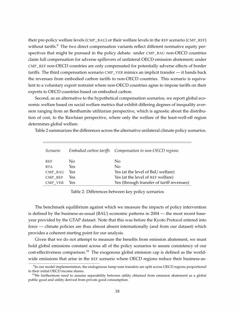
Table 2 summarizes the differences across the alternative unilateral climate policy scenarios.

Scenario Embodied carbon tariffs Compensation to non-OECD regions

REF No NoBTA Yes NoCMP_BAU Yes Yes (at the level of BaU welfare)CMP_REF Yes Yes (at the level of REF welfare)CMP_VER Yes Yes (through transfer of tariff revenues)

Table 2: Differences between key policy scenarios

The benchmark equilibrium against which we measure the impacts of policy interventionis defined by the business-as-usual (BAU) economic patterns in 2004 — the most recent base-year provided by the GTAP dataset. Note that this was before the Kyoto Protocol entered intoforce — climate policies are thus almost absent internationally (and from our dataset) whichprovides a coherent starting point for our analysis.

Given that we do not attempt to measure the benefits from emission abatement, we musthold global emissions constant across all of the policy scenarios to assure consistency of ourcost-effectiveness comparison.10 The exogenous global emission cap is defined as the world-wide emissions that arise in the REF scenario where OECD regions reduce their business-as-

9In our model implementation, the endogenous lump-sum transfers are split across OECD regions proportionalto their initial OECD income shares.

10We furthermore need to assume separability between utility obtained from emission abatement as a globalpublic good and utility derived from private good consumption.

18

usual emissions by 20%. If carbon tariffs reduce leakage then the effective reduction require-ment of OECD regions will be lower than 20%. Technically, the global emission constraintrequires an endogenous scaling of the initial 20% OECD emission pledge to match the world-wide emissions emerging from the reference scenario (REF). The costs of the emission con-straints are measured in terms of the Hicksian equivalent variation (EV) in income.

We begin our discussion of simulation results by examining how emission levels respondto alternative climate policy designs. Columns (1) and (2) of Table 3 report abatement rates byregion for the reference scenario (REF) and the uncompensated tariff scenario (BTA) relative topre-policy baseline emissions.

Because global emissions are held constant across these scenarios, the change in OECDemissions across the scenarios gives an indication of the shift in abatement responsibility be-tween OECD and non-OECD regions implied by the imposition of the tariffs in BTA. In ourcentral case simulations, the use of the tariffs relieves OECD countries on average of more than10% of their domestic abatement requirements.

Region % ∆ Emissions Leakage RateREF BTA REF BTA

(1) (2) (3) (4)

Global -7.76 -7.76 15.30 3.19OECD -20.00 -17.58 - -Non-OECD 2.59 0.54 - -

Rest of World 4.19 1.49 4.77 1.70China 1.22 0.06 2.54 0.13Russia 3.28 -0.06 1.89 -0.04OPEC 2.87 -0.15 1.88 -0.09South Africa 6.91 0.38 1.20 0.07India 1.81 0.87 0.93 0.44South Korea 2.85 2.28 0.55 0.44Indonesia 3.13 1.27 0.45 0.18Mexico 2.20 -0.09 0.36 -0.01Brazil 2.25 0.78 0.29 0.10Turkey 3.00 2.08 0.28 0.20Argentina 2.66 1.75 0.13 0.08Ethiopia 5.24 -2.58 0.01 -0.01

Table 3: Emission Responses by Region and Scenario

Looking across non-OECD regions, we see evidence of carbon leakage under REF with non-

19

OECD emissions increasing on average by 2.6% (emissions of individual non-OECD regionsincrease 1-7%) in response to the externally imposed 20% emission reduction by OECD. Tariffson embodied carbon under BTA uniformly dampen the emission increase in non-OECD regionsand thus reduce the effective abatement burden for the OECD.

Columns (3) and (4) of Table 3 describe the same emissions responses in terms of averageleakage rates — the change in each non-OECD region’s emission level divided by the cumula-tive change in emissions in OECD countries relative to the pre-policy baseline. The reductionin the leakage rates induced by the carbon tariffs is substantial. The average leakage rate forall non-OECD countries decreases from just over 15% under REF to around 3% under BTA.Thus leakage is to a large extent eliminated by the tariffs. China, OPEC and Russia, all majorcontributors to global emissions, see their leakage rates fall to approximately zero under BTA.

Table 4 reveals the differences in regional welfare costs as we move from the reference sce-nario without embodied carbon tariffs (REF) to the BTA scenario with embodied carbon tariffs(regions are ranked in descending order of their welfare losses under BTA). The top of the ta-ble summarizes the global efficiency cost of the different policies as well as the average costto OECD and non-OECD regions when we are agnostic on cost distribution. In the referencescenario, the biggest economic losses are experienced by the energy-exporting regions, Rus-sia and OPEC, despite the fact that they are not subject to emission regulation. These wel-fare cost, corresponding to around 3% of base-year consumption, are a direct consequence ofterms-of-trade changes. Carbon abatement lowers demands for fossil fuels, and this depressesthe international price of oil, coal and natural gas — products which represent a substantialshare of export earnings and GDP for Russia and OPEC. Beyond terms-of-trade changes oninternational fuel markets, OECD countries can pass on part of their cost increase in domesticenergy-intensive production to trading partners. We see that the welfare impacts for remainingnon-OECD countries (other than energy exporters Russia and OPEC) are in a similar order ofmagnitude as those experienced by abating OECD regions with India and Turkey experiencingmodest welfare gains relative to business-as-usual.

Implementation of embodied carbon tariffs without compensation as captured by scenarioBTA induces a substantial cost shifting from OECD countries to non-OECD countries. Amongthe most heavily impacted non-OECD regions are, once again, Russia and OPEC (6-7% losses).China goes from experiencing negligible welfare effects under REF to almost a 4% welfare lossunder BTA. The tariffs have a pronounced impact on relative prices, essentially operating asa monopsony markup on exports from the unregulated non-OECD countries. As a result, theindirect terms-of-trade benefits realized by OECD regions more than offset direct abatementcost for major industrialized regions such as Germany, Rest of EU, the United States and Japan.The carbon tariffs function as a sort of “back-door” trade policy for these countries, substi-tuting for optimal tariffs that would be illegal under free trade agreements. These effects arelarge enough that OECD countries on average experience net gains from climate policy relative

20

% ∆ Welfare (EV)REF BTA

Global -0.32 -0.32OECD -0.25 0.30Non-OECD -0.58 -2.48

Russia -3.28 -7.04OPEC -2.91 -6.28China -0.20 -3.85South Africa -0.20 -2.30Rest of World -0.26 -1.96Argentina -0.28 -1.83Indonesia -0.65 -1.80Mexico -0.34 -1.04Brazil 0.01 -0.72South Korea 0.24 -0.49Canada -1.00 -0.47Australia/NZ -0.59 -0.26India 0.28 -0.26Turkey 0.40 -0.05France -0.41 0.02United Kingdom -0.40 0.06Italy -0.44 0.16Japan -0.26 0.22United States -0.15 0.29Germany -0.13 0.68Rest of EU -0.19 0.79Ethiopia 0.31 0.89

Table 4: Welfare Effects by Region and Scenario

to business-as-usual for our central case simulation. Non-OECD regions are on average nega-tively impacted by unilateral OECD climate policy. However, the welfare losses become muchmore pronounced with the carbon tariffs. We see clear evidence for the concerns of developingcountries that the developed world could enact carbon tariffs as a trade policy instrument tochange terms of trade in their favor. The comparison of the global efficiency cost under REF

and BTA shows that the tariffs do yield global cost savings relative to REF but their magnitudeis very small in our central case. We return to this issue in our discussion of the sensitivityanalysis below.

Figure 5 formalizes the assessment of the distributional effects of the different policies by

21

comparing global welfare changes using social welfare functions that exhibit different degreesof inequality aversion. The general form of the social welfare function is

SWF =

[∑r

γrW(1−1/σ)r

]1/(1−1/σ)

where Wr represents the money-metric per capita welfare level in model region r, σ is theinequality aversion parameter, and γr is region r’s share of world population.

Figure 5 reports percentage changes in SWF from pre-policy baseline levels under differentassumption about the value that σ takes on. A value of σ = +∞ (“Bentham” in the figure)corresponds to the change in aggregate economic surplus, a measure of global welfare changethat is agnostic about the regional distribution of cost. A value of σ = 0 (“Rawls” in the figure)corresponds to the social welfare function

SWF = minr

(Wr)

where it is the welfare level of the poorest region that determines global welfare. (Ethopia isthe poorest country represented in the GTAP 7.1 dataset.) Entries listed in between these twoextreme cases on the x-axis of the figure describe results based on intermediate values of σ.

When we compare the alternative policies from a utilitarian perspective (“Bentham”) wefind that embodied carbon tariffs increase global cost-effectiveness of unilateral climate pol-icy. Under the Benthamite welfare metric, introducing the carbon tariffs (BTA) is cheaper thanrelying on domestic OECD abatement alone (REF) but only modestly so.

Assessing the tariff scenarios which involve explicit compensation to non-OECD regions(CMP_BAU, CMP_REF and COMP_VER) we see that compensation tilts the results based on theBenthamite welfare function back in favor of REF. Compensation increases income levels innon-OECD countries. This positive income effect raises demand for fossil energy and emission-intensive goods which results in higher leakage rates. Holding global emissions constant at theREF level requires more domestic abatement efforts on the part of OECD regions, raising theoverall cost of these policies.

Finally, we evaluate the welfare impacts of alternative unilateral climate policy designsfor different forms of the social welfare function. We find that the welfare cost of BTA risessubstantially as inequality aversion becomes a more important element of the welfare criteria.This reflects the finding that OECD tariffs shift emission abatement cost to non-OECD countriesvia a deterioration of the terms of trade. As non-OECD countries represent the poorer partin the global economy, the burden shifting of unilateral climate policy towards these regionsexacerbates pre-existing inequalities. Interestingly, this pattern is interrupted as σ approacheszero in the social welfare function because the poorest region in the model, Ethiopia, actually

22

-2.5

-2

-1.5

-1

-0.5

0

0.5

1

1.5

2

%

Social Welfare Metric

BTA

REF

CMP_BAU

CMP_REF

CMP_VER

Figure 5: % Change in Global Welfare by Social Welfare Function and Scenario

benefits from terms-of-trade gains — mainly through reduced expenditures for energy imports.Naturally, the various compensation scenarios fare better than BTA as inequality aversion

become important. CMP_REF yields similar welfare changes to REF because non-OECD coun-tries are, by definition, compensated to REF welfare levels. CMP_BAU and CMP_VER do evenbetter because the scope for compensation to non-OECD countries increases. Note, however,that these results are more of a statement about the potential for improving standards of livingin non-OECD countries through wealth transfers than they are evidence of the effectiveness ofembodied carbon tariffs.

Past studies of carbon leakage based on CGE simulations show that magnitude of leakageis sensitive to a few key model assumptions. First, the larger is the unilateral cutback in emis-sions that is assumed in the model, the stronger is the leakage effect as abating regions move toincreasingly inelastic portions of the demand curve for emission-intensive goods. Second, thehigher are the Armington elasticities that determine how substitutable varieties of emission-

23

intensive goods from different countries are, the stronger is the leakage effect as regions maymore easily substitute to new sources for these goods in response to the changes induced bythe climate policy regime. Finally, the lower are the fossil-fuel supply elasticities that are as-sumed in the model, the stronger is the leakage effect as the decreased demand for fossil fuelsin abating regions produces larger reductions in the price of these goods on world markets,stimulating demand abroad.

We have performed comprehensive sensitivity analysis with respect to all three of theseassumptions to test how they alter our conclusions regarding the effectiveness of the carbontariffs. Table 5 summarizes our main findings. The table depicts the average leakage rate pro-duced by the model under the REF scenario (“REF Leakage Rate” in the table) and the differencein the global cost of the REF and the BTA scenarios as a percentage of global consumption (“BTA-REF Cost Savings” in the table) for three alternative leakage scenarios. The first three columnsof the table describe the alternative assumptions underlying the leakage scenarios we model.The table shows the percentage cutback assumed and the values that the Armington and fossilfuel supply elasticities take on relative to their values in the central case that our discussion hasfocused on up to this point.

Cutback Armington Supply REF BTA-REF

Elasticities Elasticities Leakage Rate Cost Savings

10% 1/2x 2x 6.86 0.01120% 1x 1x 15.30 0.00430% 2x 1/2x 30.64 0.097

Table 5: Leakage Sensitivity Analysis

The leakage rate produced by the model is increasing as we move down the rows of thetable. The leakage rates produced by the model are approximately 7% and 15% in the low andmedium-leakage scenarios, respectively. The cost savings are close to zero in both of these sce-narios — less than 0.02 percent of world consumption and approximately 1 percent of the totalREF policy cost. The leakage rate increases to approximately 30% in the high-leakage scenarioand the cost savings are larger in this case — approximately 0.1 percent of world consumptionor 12% of the total cost of the REF policy. Thus, we find that there may be measurable efficiencygains from the tariffs for policy scenarios that produce higher levels of leakage than those re-ported in our central case. It is worth noting, however, that when we repeat the exercise withthe social welfare functions described in Figure 5 using the assumptions of the high-leakagescenario, the efficiency gains produced by the use of the tariffs are not sufficient to overturn theranking of the policies we established for the central case. That is, the BTA scenario produces

24

larger global welfare losses than the reference policy for all of the welfare metrics that exhibitinequality aversion.

7 Conclusions

In the international climate policy debate, the idea of imposing tariffs on embodied carbon hasattracted significant attention in OECD countries contemplating unilateral emission reductions.The basic idea is to combine domestic carbon taxes or cap-and-trade systems that cover directemissions in production with tariffs on the embodied carbon of goods imported from non-abating trade partners. From a theoretical perspective, the measures could serve as a second-best instrument to improve cost-effectiveness of unilateral climate policies.

In our quantitative experiments, we find that the carbon tariffs are quite effective in reduc-ing carbon leakage from unilateral OECD policies. However, the efficiency gains from carbontariffs are modest even under our optimistic assumption that the tariffs cover all sectors andcan be levied on the full embodied carbon content without transaction costs.

The tariffs are a clear winner from the perspective of those countries implementing themand quite damaging to many of the countries subject to them. Many major OECD membersexperience net gains from implementing climate policy when tariffs are used but, from an dis-tributional perspective, the tariffs exacerbate pre-existing income inequality, and the modestglobal cost savings provided by border tariffs quickly evaporate as inequality aversion is takeninto account.

It would be difficult to overstate the influence that the divide between the perspectives ofdeveloped and developing-world nations has exerted on the international climate policy pro-cess to date. Developing countries argue that they cannot accept binding emissions targets un-der any equitable climate policy regime. Major developed countries, notably the United States,argue that they cannot accept binding targets for fear that their abatement efforts will be un-dermined by carbon leakage if their developing-world partners are not subject to comparablerestrictions.

In light of this tension, the decision to use embodied carbon tariffs — by punishing thedeveloping-world countries subjected to them — could be quite destructive to the existing pol-icy process. In the extreme, it could even result in a tariff war. A different view is that tariffsmight function as a political stick in the drive to commit intransigent countries to adopt emis-sion restrictions. They have the appeal of (i) being a credible threat, since OECD membersbenefit from their use while being very damaging to those countries subject to them, and (ii)carrying a certain moral stamp of approval because they are being used in the name of envi-ronmental policy and appear to have the potential to reduce carbon leakage.

A logical next step in the analysis we have carried out here would be to consider howcountries subjected to embodied carbon tariffs might respond and what actions they would be

25

willing to undertake to avoid the tariffs in the first place.

26

Acknowledgements

This research has been supported by Environment Canada. Research assistance has been pro-vided by Justin Carron. The views expressed here and any errors are our own.

27

References

Armington, Paul S., “A Theory of Demand for Producers Distinguished by Place of Produc-tion,” IMF Staff Papers, 1969, 16 (1), 159–78.

Babiker, Mustafa H., “Climate change policy, market structure and carbon leakage,” Journal ofInternational Economics, 2005, 65 (2), 421–45.

Babiker, Mustafa H and Thomas F Rutherford, “The Economic effects of Border Measures inSubglobal Climate Agreements,” The Energy Journal, 2005, 26 (4), 99–126.

Böhringer, Christoph and Andreas Löschel, “Assessing the Costs of Compliance: The KyotoProtocol,” European Environment, 2002, 12 (1), 1–16.

and Thomas F. Rutherford, “Carbon Abatement and International Spillovers,” Environ-mental and Resource Economics, 2002, 22 (3), 391–417.

and , “Who should pay and how much? Compensation for International Spilloversfrom Carbon Abatement Policies to Developing Countries — A Global CGE Assessment,”Computational Economics, 2004, 23 (1), 71–103.

and , “The Cost of Compliance: A CGE Assessment of Canada’s Policy Optionsunder the Kyoto Protocol,” World Economy, 2010, 33 (2), 177–211.

, Carolyn Fischer, and Knut E. Rosendahl, “The Global Effects of Subglobal Climate Poli-cies,” The B.E. Journal of Economic Analysis and Policy, 2010, 10 (2), Article 13.

, Thomas F. Rutherford, and Alfred Voss, “Global CO2 Emissions and Unilateral Action:Policy Implications of Induced Trade Effects,” International Journal of Global Energy Issues,1998, pp. 18–22.

Brewer, Thomas L., “U.S. Climate Policy and International Trade Policy Intersections: IssuesNeeding Innovation for a Rapidly Expanding Agenda,” Technical Report, Center for Busi-ness and Public Policy, Georgetown University February 2008.

Brooke, Anthony, David Kendrick, and Alexander Meeraus, GAMS: A User’s Guide 1996.

Burniaux, Jean-Mark and Joaquim Oliveira Martins, “Carbon Emission Leakage: A GeneralEquilibrium View,” Working Paper 242, Economics Department, Organisation for Eco-nomic Co-operation and Development 1999.

Bushnell, James, Carla Peterman, and Catherine Wolfram, “Local Solutions to Global Prob-lems: Climate Change Policies and Regulatory Jurisdiction,” Review of Environmental Eco-nomics and Policy, 2008, 2, 175–193.

28

Charnowitz, Steve, Gary Clyde Hufbauer, and Jisun Kim, “Global Warming and the WorldTrading System,” Technical Report, Peterson Institute for International Economics 2009.

Copeland, Brian R. and M. Scott Taylor, “Trade, Growth and the Environment,” Journal ofEconomic Literature, 2004, XLII, 7–71.

Dirkse, Steve and Michael Ferris, “The PATH Solver: A Non-Monotone Stabilization Schemefor Mixed Complementarity Problems,” Optimization Methods & Software, 1995, 5, 123–56.

Felder, Stefan and Thomas F. Rutherford, “Unilateral Reductions and Carbon Leakage. TheEffect of International Trade in Oil and Basic Materials,” Journal of Environmental Economicsand Management, 1993, 25, 162–176.

Fischer, Carolyn and Alan Fox, “Comparing Policies to Combat Emissions Leakage: BorderTax Adjustements versus Rebates,” RFF discussion paper, 2009, RRF DP 09-02.

Graham, Paul, Sally Thorpe, and Lindsay Hogan, “Non-competitive market behavior in theinternational coking coal market,” Energy Economics, 1999, 21, 195–212.

Ho, Mun S., Richard Morgenstern, and Jhih-Shyang Shih, “Impact of Carbon Price Policieson U.S. Industry,” Technical Report, Resources For the Future December 2008.

Hoel, Michael, “Global Environmental Problems: The Effects of Unilateral Actions Taken byOne Country,” Journal of Environmental Economics and Managament, 1991, 20, 55–70.

, “Should a carbon tax be differentiated across sectors?,” Journal of Public Economics, 1996,59, 17–32.

Houser, Trevor, Rob Bradley, and Britt Childs, “Leveling the Carbon Playing Field, Interna-tional Competiton and US Climate Policy Design,” Peterson Institute for International Eco-nomics, World Resources Institute: Washington DC., 2008.

Howse, Robert and Antonia L. Eliason, “Domestic and International Strategies to AddressClimate Change: An Overview of the WTO Legal Issues,” International Trade Regula-tion and the Mitigation of Climate Change. Cambridge University Press., 2008.

ICTSD, “Climate Change: Schwab Opposes Potential Trade Measures,” Bridges Trade BioRes,March 2008, 8 (4).

Krichene, Noureddine, “World crude oil and natural gas: a demand and supply model,” En-ergy Economics, 2002, 24, 557–576.

Markusen, James R., “International Externalities and Optimal Tax Structures,” Journal of Inter-national Economics, 1975, 5, 15–29.

29

Mattoo, Aaditya, Arvind Subramanian, Dominique Van Der Mensbrugghe, and Jianwu He,“Reconciling Climate Change and Trade Policy,” World Bank Policy Research Working PaperNo. 5123, 2009.

McKibbin, Warwick J. and Peter J. Wilcoxen, “The Economic and Environmental Effects ofBorder Tax Adjustments for Climate Policy,” Working Paper - Syracuse University, 2008.

Narayanan, Badri and Terrie L. Walmsley, “The GTAP 7 Data Base Documentation,” TechnicalReport, Purdue University, Center for Global Trade Analysis 2008.

Okagawa, Azusa and Kanemi Ban, “Estimation of Substitution Elasticities for CGE Models,”mimeo, Osaka University April 2008.

Paltsev, Sergey V., “The Kyoto Protocol: Regional and Sectoral Contributions to the CarbonLeakage,” Energy Journal, 2001, 22 (4), 53–79.

Pauwelyn, Joost, “US Federal climate policy and competitiveness concerns: the limits andoptions of international trade law,” Duke University working paper, 2007.

Peters, Glen P. and Edgar G. Hertwich, “CO2 Embodied in International Trade with Implica-tions for Global Climate Policy,” Environmental Science & Technology, March 2008, 42 (5),1401–1407.

and , “Post-Kyoto greenhouse gas inventories: production versus consumption,”Climatic Change, 2008, 86, 51–66.

and , “Trading Kyoto,” Nature Reports Climate Change, 2008, 2, 40–41.

Shoven, John B. and John Whalley, Applying general equilibrium, Cambridge University Press,1992.

United Nations, Text of the Kyoto Protocol, United Nations Framework Convention on ClimateChange, 1997.

Weber, Christopher L. and H. Scott Matthews, “Embodied Environmental Emissions in U.S.International Trade, 1997-2004,” Environmental Science and Technology, 2007, 41, 4875–4881.

Whalley, John and Ben Lockwood, “Carbon-motivated Border Tax Adjustments: Old Wine inGreen Bottles?,” World Economy, 2010, 33 (6), 810–9.

30

A MRIO Recursive Solution Algorithm

The estimate in iteration k + 1 is a simple refinement of the estimate in iteration k

xk+1 = b+Axk

Iterative solution of the MRIO model involves the following steps:

Initialize:xygr = co2egr/vomgr

Repeat: i. Refine estimates of the embodied carbon of international trade services:

xtj =

∑r vstjrx

yjr

vtwj

ii. Refine estimates of the embodied carbon of bilateral imports:

xmir =

∑s

(vxmdisrx

yis +

∑j x

tjvtwrjisr

)vimir

iii. Update embodied carbon estimates:

xygr =co2gr +

∑i x

mirvifmigr +

∑i x

yirvdfmigr

vomgr

31

B Algebraic Description of the CGE Model

The computable general equilibrium model is formulated as a system of nonlinear inequalities.The inequalities correspond to the two classes of conditions associated with a general equilib-rium: (i) exhaustion of product (zero profit) conditions for constant-returns-to-scale producers;and (ii) market clearance for all goods and factors. The former class determines activity levelsand the latter determines price levels. In equilibrium, each of these variables is linked to oneinequality condition: an activity level to an exhaustion of product constraint and a commodityprice to a market clearance condition.

In our algebraic exposition, the notation is used to denote the unit profit function (calculatedas the difference between unit revenue and unit cost) for constant-returns-to-scale productionof sector i in region r where z is the name assigned to the associated production activity. Differ-entiating the unit profit function with respect to input and output prices provides compensateddemand and supply coefficients (Hotelling’s Lemma), which appear subsequently in the mar-ket clearance conditions. We use g as an index comprising all sectors/commodities i (g = i),the final consumption composite (g = C), the public good composite (g = G), and aggregateinvestment (g = I). The index r (aliased with s) denotes regions. The index EG represents thesubset of all energy goods (here: coal, oil, gas, electricity) and the label FF denotes the subsetof fossil fuels (here: coal, oil, gas). Tables 6 - 11 explain the notation for variables and parame-ters employed within our algebraic exposition. Figures 6 - 8 provide a graphical exposition ofthe production structure. Numerically, the model is implemented in GAMS (Brooke, Kendrickand Meeraus 1996) and solved using PATH (Dirkse and Ferris 1995).

Zero-profit conditions:

• Production of goods except fossil fuels (g /∈ FF ):

ΠYgr = pgr−

θMgrpM(1−σKLEMgr )gr + (1− θMgr)

[θEgrp

E(1−σKLEgr )gr + (1− θEgr)p

KL(1−σKLEgr )gr

] (1−σKLEMgr )

(1−σKLEgr )

1/(1−σKLEMgr )

≤ 0

• Sector-specific material aggregate:

ΠMgr = pMgr −

[ ∑i/∈EG

θMNigr p

A(1−σMgr)igr

]1/(1−σMgr)≤ 0

• Sector-specific energy aggregate:

ΠEgr = pEgr −

[ ∑i∈EG

θENigr (pAigr + pCO2r aCO2

igr )(1−σEgr)

]1/(1−σEgr)≤ 0

32

• Sector-specific value-added aggregate:

ΠKLgr = pKLgr −

[θKgrv

(1−σKLgr )gr + (1− θKgr)w

(1−σKLgr )r

]1/(1−σKLgr )

≤ 0

• Production of fossil fuels (g ∈ FF ):

ΠYgr = pgr −

θQgrq(1−σQgr)gr + (1− θQgr)

(θLgrwr + θKgrvgr +

∑i/∈FF

θFFigr pAigr

)(1−σQgr)1/(1−σQgr)

≤ 0

• Armington aggregate:

ΠAigr = pAigr −

(θAigrp

(1−σAir)ir + (1− θAigr)p

IM(1−σAir)ir

)1/(1−σAir)≤ 0

• Aggregagte imports across import regions:

ΠIMir = pIMir −

[∑s

θIMisr p(1−σIMir )is

]1/(1−σIMir )

≤ 0

Market-clearance conditions:

• Labor:

Lr ≥∑g

Y KLgr

∂ΠKLgr

∂wr

• Capital:

Kgr ≥ Y KLgr

∂ΠKLgr

∂vgr

• Fossil fuel resources (g ∈ FF ):

Qgr ≥ Ygr∂ΠY

gr

∂qgr

• Material composite:

Mgr ≥ Ygr∂ΠY

gr

∂pMgr

• Energy composite:

Egr ≥ Ygr∂ΠY

gr

∂pEgr

• Value-added composite:

KLgr ≥ Ygr∂ΠY

gr

∂pKLgr

33

• Import composite:

IMir ≥∑g

Aigr∂ΠA

igr

∂pIMir

• Armington aggregate:

Aigr ≥ Ygr∂ΠY

gr

∂pAigr

• Commodities (g = i):

Yir ≥∑g

Aigr∂ΠA

igr

∂pir+∑s 6=r

IMis∂ΠIM

is

∂pir

• Private consumption (g = C):

YCrpCr ≥ wrLr +∑g

vgrKgr +∑i∈FF

qirQir + pCO2r

¯CO2r + Br

• Public consumption (g = G):

YGr ≥ Gr

• Investment (g = I):

YIr ≥ Ir

• Carbon emissions:

¯CO2r ≥∑g

∑i∈FF

Egr∂ΠE

gr

∂(pAigr + pCO2r aCO2

igr )aCO2igr

34

i, j Sectors and goods

g The union of produced goods i, private consumption C,public demand G and investment I

r, s Regions

EG Energy goods; coal, crude oil, refined oil, natural gas andelectricity

FF Fossil fuels; coal, crude oil and natural gas.

Table 6: Indices & Sets

Ygr Production of item g in region r

Egr Energy composite for item g in region r

KLgr Value-added composite for item g in region r

Aigr Armington aggregate for commodity i for demand category(item) g in region r

IMir Aggregate imports of commodity i in region r

Table 7: Activity Levels

35

pgr Price of item g in region r

pMgr Price of material composite for item g in region r

pEgr Price of energy composite for item g in region r

pKLgr Price of value-added composite for item g in region r

pAigr Price of Armington good i for demand category g in regionr

pIMir Price of import composite for good i in region r

wr Wage rate in region r

vir Capital rental rate in sector i in region r

qir Rent to fossil fuel resources in region r (i ∈ FF )

pCO2r Implicit price of carbon in region r

Table 8: Prices

Lr Aggregate labor endowment for region r

Kir Capital endowment for sector i in region r

Qir Endowment of fossil energy resource i in region r (i ∈ FF )

Br Initial balance for payment deficit or surplus in region r(note:

∑r Br = 0)

¯CO2r Aggregate carbon emission cap in region r

aCO2igr Carbon emission coefficient for fossil fuel i in demand cate-

gory g in region r (i ∈ FF )

Table 9: Endowments and Carbon Emissions Specification

36

θMgr Cost share of material composite in production of item g inregion r

θEgr Cost share of energy composite in the aggregate of energyand value added of item g in region r

θMNigr Cost share of material input i in the material composite of

item g in region r

θENigr Cost share of energy input in the energy composite of item gin region r

θKgr Cost share of capital within the value-added composite ofitem g in region r

θQgr Cost share of fossil fuel resource in fossil fuel production(g ∈ FF ) in region r

θLgr Cost share of labor in non-resource inputs to fossil fuel pro-duction (g ∈ FF ) in region r

θKgr Cost share of capital in non-resource inputs to fossil fuel pro-duction (g ∈ FF ) in region r

θFFigr Cost share of good i in non-resource inputs to fossil fuel pro-duction (g ∈ FF ) in region r

θAigr Cost share of domestic output i within the Armington itemg in region r

θMisr Cost share of exports of good i from region s in the importcomposite of good i in region r

Table 10: Cost Share Parameters

37

σKLEMgr Substitution between the material composite and theenergy-value-added aggregate in the production of item gin region r*

σKLEgr Substitution between energy and the value-added compos-ite in the production of item g in region r*

σMgr Substitution between material inputs within the energycomposite in the production of item g in region r*

σKLgr Substitution between capital and labor within the value-added composite in the production of item g in region r*

σEgr Substitution between energy inputs within the energy com-posite in the production of item g in region r (by default= 0.5)

σQgr Substitution between natural resource input and the com-posite of other inputs in the fossil fuel production (g ∈ FF )of region r***

σIMir Substitution between imports from different regions withinthe import composite for good i in region r**

* — Calibrated based on estimates from Okagawa and Ban (2008).** — Calibrated based on estimates from Narayanan and Walmsley (2008).*** — Calibrated based on estimates from Graham et al. (1999) and Krichene (2002).

Table 11: Elasticity Parameters

38

Figure 6: Nesting in Non-Fossil-Fuel Production

Figure 7: Nesting in Fossil-Fuel Production

Figure 8: Nesting in Armington Composite Production

39