Ellsberg Paradox: Ambiguity and Complexity

Aversions Compared∗

Jaromır Kovarık†’‡ Dan Levin§ Tao Wang¶

January 16, 2016

Abstract

We present a simple model where preferences with complexity aver-sion, rather than ambiguity aversion, resolve the Ellsberg paradox. Wetest our theory using laboratory experiments where subjects choose amonglotteries that “range” from a simple risky lottery, through risky but morecomplex lotteries, to one similar to Ellsberg’s ambiguity urn. Our modelranks lotteries according to their complexity and makes different–at timescontrasting–predictions than most models of ambiguity in response to ma-nipulations of prizes. The results support that complexity aversion pref-erences play an important and separate role from beliefs with ambiguityaversion in explaining behavior under uncertainty.

Keywords: Ambiguity, Complexity, Compound Risk, Ellsberg paradox, Risk,Uncertainty.JEL Classification: C91, D01, D81.

∗Our paper greatly benefited from comments and suggestions of a referee and the Editor.We also thank Itzhak Gilboa, Yoram Halevy, Brian Hill, Dimitry Mezhvinsky, Jim Peck, andparticipants of the DT conference 2009 in HCE Paris and SEET 2013. Jaromır Kovarıkgreatly acknowledges support from Spanish Ministry of Science and Innovation (ECO 2012-31626, ECO 2012-35820), the Basque Government (IT-783-13), and GACR (14-22044S).†Dpto Fundamentos Analisis Economico I & Bridge, University of the Basque Country,

Av. Lehendakari Aguirre 83, 48015 Bilbao, Spain (jaromir.kovarik@ehu.es).‡CERGE-EI, a joint workplace of Charles University in Prague and the Economics Institute

of the Czech Academy of Sciences, Politickych veznu 7, 111 21 Prague, Czech Republic.§Department of Economics, The Ohio State University, 1945 North High Street, Columbus,

OH 43210 (levin.36@osu.edu).¶Department of Economics, Swarthmore College, 500 College Avenue, Swarthmore, PA

19081-1397.

1

1 Introduction

In his thought experiment, Ellsberg (1961) offered subjects (some of whom wererenowned economists) a bet on red (black) that paid a high prize if the colordrawn from the chosen urn was red (black). Subjects had to choose between twourns. Urn I contained 100 red and black balls in an unknown ratio and urn IIcontained exactly 50 red and 50 black balls. A significant percentage of subjectschose urn II in both the bet on red and the bet on black, violating principlesimplied by Savage’s (1954) expected utility theory (EUT) as these choices couldnot be rationalized by any subjective prior distribution of the states of theworld envisioned by EUT. Ellsberg’s paradox highlighted that Savage’s axioms,the sure-thing principle in particular, are quite restrictive and that there is aneed for a revised or even new theory of decision making under uncertainty. Avariety of models have been developed to generalize EUT and resolve Ellsberg’sparadox so far (see Gilboa and Marinacci (2013) for an excellent review).1 Thisliterature mostly focuses on the principles governing the formulation of beliefs,with little attention to the possible direct impact of uncertainty/ambiguity onutilities.

In contrast, we recognize that, say, a prize of $10 from an ambiguous urnmay not be viewed as equivalent to a prize of $10 from a simpler decision prob-lem (risky urn) and provide a simple alternative explanation to the Ellsberg’sparadox. We argue that choices that seem to contradict the existence of a priordistribution could have been made by subjects who do have a prior distribu-tion of the different states of nature, but who are averse to complexity andregard it as a cost that taxes the utility of the lottery.2 Having a diffuse priorover the (101) different states of nature in Ellsberg’s urn transforms it into arisky but compound lottery.3 In addition, our complexity-averse decision mak-ers (DMs) do not regard compound lotteries as equivalent to their reduced formcounterparts. As a result, the Ellsberg paradox can be explained by complexityaversion that is applied to utilities and not beliefs as in (most of) the literatureon ambiguity aversion.

Recently, Halevy (2007) has documented a strong association between atti-tudes to ambiguity and the failure to reduce compound (objective) lotteries (seealso Dean and Ortoleva (2011) and Abdellaoui et al. (2011)), suggesting thatthe failure to reduce compound lotteries might be one contributing factor of theEllsberg paradox. However, this work was not designed to disentangle whether

1Leading theories include Schmeidler (1989), Gilboa and Schmeidler (1989), Segal (1987,1990), and more recently Klibanoff et al (2005) and Maccheroni et al. (2006). Section 2 andOnline Appendix A provide a more detailed exposition of these theories in the context of ourexperiment.

2Modeling complexity aversion as taxing utilities due to the extra (cognitive) costly effortto compute reduced-form equivalents would result in a circular argument. The reason is that,once such effort is already taken, it becomes sunk and should not affect choices. However, we donot assume that DMs reduce the lotteries, and our simple model and treatment manipulationsenable us to distinguish complexity from uncertainty aversion. See below.

3We model the DM as having a particular prior on the Ellsberg urn lottery only to illustrateour claim: There do exist priors with complexity aversion that resolve the Ellsberg paradox.

2

and/or to what extent uncertainty/ambiguity affects DMs through beliefs orutility.

Our theory generates several predictions, some of which contrast with pre-vious literature. First, it induces a ranking of alternatives that exhibit the samedegree of riskiness but differ in their complexity or compoundness. Second, themodel generates predictions of DMs’ response to prize manipulations that dif-fer from the literature on ambiguity and we design an experiment that enablesus to distinguish between complexity aversion and the leading theories of un-certainty/ambiguity aversion. Some of our findings are statistically weak, yetoverall they support the idea that complexity aversion should be viewed as animportant and a separate force from ambiguity aversion.4

We do not provide a formal definition of complexity or a way to measureit. Instead, we relate complexity in our experiment to the compoundness (thenumber of layers) and the number of alternatives (branches) of the lotteries.Note that Ellsberg did not provide a formal measure of ambiguity or its aversion.Instead, he called attention to what seems like a paradox under EUT that theliterature, for over 50 years, had tried to resolve by focusing on new beliefformation. In contrast, we offer an alternative (additional) explanation viacomplexity aversion that affects the utility but not beliefs.

We neither dispute the significance of Ellsberg’s observation nor the valu-able contribution of the research on uncertainty/ambiguity, nor argue that ourtheory replaces approaches that are based on belief formations. The argumentwe envision here is that complexity aversion may play a relevant, distinct, andimportant role alongside uncertainty/ambiguity aversion and thus deserves at-tention. Since we find evidence of complexity aversion, disentangling the indi-vidual principles behind the Ellsberg paradox (e.g. Ahn et al., 2014) or evaluat-ing the performance of different models of ambiguity aversion (such as Halevy,2007) becomes more challenging as the impact of ambiguity on beliefs might beconfounded with the effects of complexity on utilities.

Our model can explain a phenomenon reported recently by Chew et al.(2013). Consider an Ellsberg-like urn with 100 balls where there are only eithern ≥ 50 or 100 − n red balls with unknown probabilities. This spans an unam-biguous risky urn if n = 50, any ambiguous urn with two possible amounts ofred balls if n ∈ (50, 100), and the extreme situation with either all balls redor all black (n = 100). As n increases from n = 50 (the risk case) to 100,Chew et al (2013) find that the willingness to pay for those lotteries declineswith n in line with some ambiguity aversion theories. However, for n = 100 thewillingness to pay sharply increases and this lottery is indistinguishable fromthe risky n = 50 one. Note that all the uncertainty resolves in one stage inthe n = 100 lottery, making this ambiguous option basically non-compound.5

Thus, since complexity scales with the compoundness, complexity aversion pre-

4The results of Halevy (2007) and Abdellaoui et al. (2011) are generally in line with theidea that people rank prospects according to their complexity. See also Yates and Zukowsky(1976).

5In contrast, the urns with n ∈ (50, 100) can be viewed as twice compound and thus morecomplex lotteries.

3

dicts the n = 50 and n = 100 urns to be similar and both to be preferred to then ∈ (50, 100) variations.

In Section 2, we describe complexity aversion and derive the experimentalhypotheses. We present our experimental design in Section 3 and the results inSection 4. Section 5 concludes. Some additional material can be found in theOnline Appendix.

2 Hypotheses

2.1 Complexity Aversion

We argue that people dislike complexity. Complexity-averse individuals tax theoutcomes of complex lotteries by a constant δ > 0. Consequently, when a DMfaces a complex lottery with two final prizes H and L, H > L ≥ 0, she viewsthe lottery as having prizes H − δ and L − δ. We assume that the parameterδ scales up with the complexity of the lottery. Hence, if a complexity-averseDM is presented with a choice between two lotteries with identical prizes andprobabilities with one lottery being a compound variation of the second, shemight prefer the latter only because of the increased complexity of the former.6

Throughout the paper, we assume that subjective probabilities coincide withobjective probabilities if they are known. In the present theory, ambiguous lot-teries are viewed by DMs as compound and more complex versions of riskylotteries, for which the corresponding probabilities can be calculated.7 For in-stance, the ambiguous Ellsberg urn can be viewed as a risky lottery in whichthere is a uniform probability of each possible number of red/black balls in theurn. This way, the Ellsberg’s urn represents a relatively complex risky lotteryand complexity-averse DMs might choose risky lotteries over ambiguous urnsbecause of the complexity involved in the computation of expectations corre-sponding to Ellsberg’s urn.

Since complexity is understood as an ordinal measure here, the presenttheory allows for a preference ranking over lotteries that are identical in both thefinal outcomes and their corresponding probabilities, but differ in the way theyare compounded and one can analyze such preference ranking in a populationusing experimental techniques.

We focus on a simple version of complexity aversion. We assume that peo-ple dislike the cognitive effort associated with computation of probabilities incomplex lotteries and avoid performing them. Instead, they estimate (or guess)the probabilities and discount the final prizes of these lotteries.

Consider a choice between a pure risky lottery A and its more complexcounterpart B, which both give high prize H with probability one half andL otherwise.8 The DM does not make the calculation of probabilities in the

6We use the linear, additive structure for expositional simplicity. However, qualitativeresults will not change with any utility that is declining in δ.

7This approach is also taken by e.g. Segal (1987) or Klibanoff et al. (2005).8We use one half for expositional simplicity. The arguments extend for different probability

levels.

4

complex lottery, but forms an estimate θ about the probability of drawing H inlottery B. Then, B � A if9

θ(H − δ) + (1− θ)(L− δ) > 1

2(H + L)

or

θ > θ∗ =1

2+

δ

H − L.

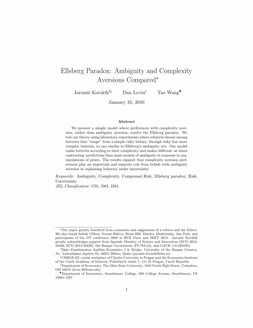
We assume that there is a distribution of θ in the population (as in Figure1a) and that the mode of the distribution is equal to the true probability (onehalf in our example).10 People whose estimated θ lies below the threshold θ∗

prefer the simpler lottery A, but a possibly non-negligible amount of people,whose beliefs about the probability of the high prize in the complex lottery Bare large enough, might prefer the more complex B to A. In addition, since θ∗

is increasing in δ and decreasing in (H − L), the fraction of people who preferB to A decreases with the complexity of B and increases with the differencebetween the high and low prizes. These observations generate two questions.

Question 1 (complexity aversion): Do most people prefer the risky lot-tery to its compound or ambiguous variations and does a non-negligible fractionof subjects still prefer the latter?

Note that, if one allows for subjective priors over the ambiguous events inthe existing theories of ambiguity aversion, any theory allows ambiguity-averseindividuals to prefer the ambiguous urn if they believe that the high prize islikely enough (see Online Appendix A for formal analysis). Hence, even if ourtheory predicts a non-negligible amount of people to prefer B, Question 1 doesnot allow us to distinguish our complexity aversion from other models.

Question 2 (degree of complexity): Does the number of people prefer-ring the risky lottery A to B increase with the complexity of B?

It is the second question that allows the testing our theory vis-a-vis othermodels explaining Ellsberg’s paradox. An important implication of complexityaversion is that the ranking of lotteries will depend on their complexity evenif they are payoff-equivalent and even if only objective risk is involved. Anytheory in which people reduce compound lotteries predicts that people shouldbe indifferent between reduced lotteries and their compound variations, thuspredicting the same number of people preferring A to B independently of theircomplexity. The differentiation of payoff-equivalent non-ambiguous lotteries re-quires a two-stage approach toward risk and uncertainty as in rank-dependent

9Note that δ in fact measures the difference in complexity between A and B, rather thanbeing an absolute measure of complexity of lottery B.

10Obviously, the complexity of the lottery itself may shape this distribution through thevariance of the estimates in the population. This, however, does not affect any of the predic-tions below.

5

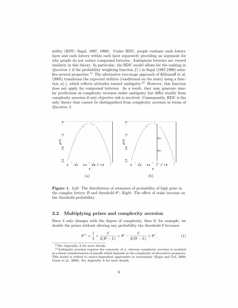
utility (RDU; Segal, 1987, 1990). Under RDU, people evaluate each lotterylayer and each lottery within each layer separately providing an argument forwhy people do not reduce compound lotteries. Ambiguous lotteries are viewedsimilarly in this theory. In particular, the RDU model allows for the ranking inQuestion 1 if the probability weighting function f(.) in Segal (1987,1990) satis-fies several properties.11 The alternative two-stage approach of Klibanoff et al.(2005) transforms the expected utilities (conditional on the state) using a func-tion φ(.), which reflects attitudes toward ambiguity.12 However, this functiondoes not apply for compound lotteries. As a result, they may generate simi-lar predictions as complexity aversion under ambiguity but differ starkly fromcomplexity aversion if only objective risk is involved. Consequently, RDU is theonly theory that cannot be distinguished from complexity aversion in terms ofQuestion 2.

(a) (b)

Figure 1. Left : The distribution of estimates of probability of high prize inthe complex lottery B and threshold θ∗; Right : The effect of stake increase onthe threshold probability.

2.2 Multiplying prizes and complexity aversion

Since δ only changes with the degree of complexity, then if, for example, wedouble the prizes without altering any probability the threshold θ becomes

θ∗∗ =1

2+

δ

2(H − L)= θ∗ − δ

2(H − L)< θ∗. (1)

11See Appendix A for more details.12Ambiguity aversion requires the concavity of φ, whereas complexity aversion is modeled

as a linear transformation of payoffs which depends on the complexity of alternative prospects.This model is related to source-dependent approaches to uncertainty (Ergin and Gul, 2009;Grant et al., 2009). See Appendix A for more details.

6

In words, if we double all of the lottery prizes, the threshold θ that makespeople indifferent between choosing the simple risky lottery over its complex(e.g. compound) “cousin” is lower and, hence, the fraction of the populationselecting the complex lottery ought to increase. Figure 1b illustrates this effectgraphically. If in particular B is an ambiguous urn, such prediction contrastsstarkly with most of the belief-based explanations of the Ellsberg paradox (seebelow).

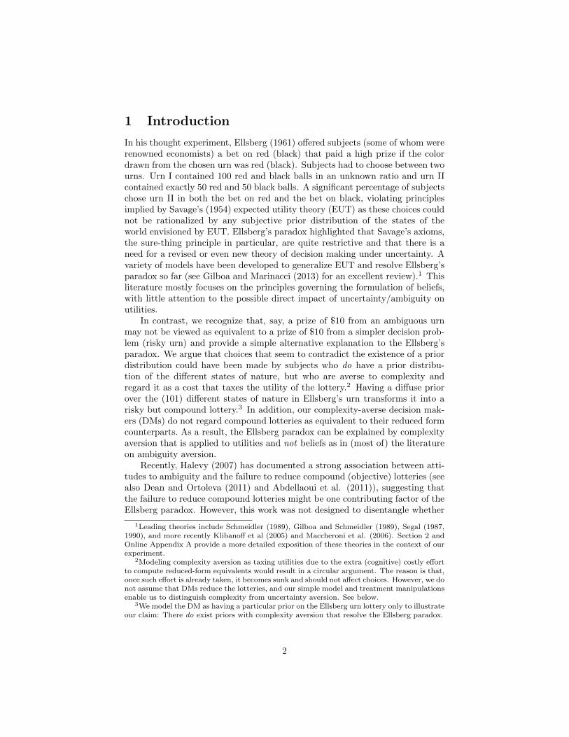
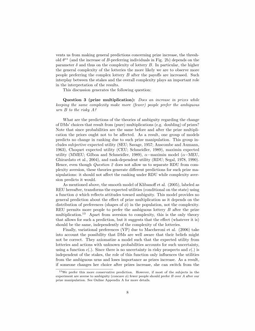
Notice that the above prediction abstracts from the possibility that, if moreis at stake (i.e. prizes are multiplied by a factor larger than one), DMs may exertmore effort in forming their probability estimates in more complex lotteries.That is, larger stakes provide an incentive to “think harder” and may result in adistribution of estimates that is more concentrated around the true probabilities(see Figure 2a).

(a) (b)

Figure 2. Left : Effect of increased effort while estimating the probability ofthe high prize in complex lotteries. Right : If stakes are multiplied and effortincreased, the difference between the mass of people that prefer B to A isgiven by (i) people who switch from A to B due to the lowering of θ∗ to θ∗∗

(area A) and (ii) people who switch from B to A due to a better estimate ofthe true probability (area B).

Figure 2 reveals that complexity aversion and the increased effort estimatingthe probability of the high prize work one against the other. The reduction ofthe threshold θ (from θ∗ to θ∗∗) increases the mass of people who prefer thecomplex/ambiguous lottery (area A in Figure 2b), while the shrinkage of tailsof the distribution due to higher effort decreases the number of B-preferringindividuals (area B in Figure 2b). Since the potential higher effort works againstthe above prediction of more people preferring B after the prize multiplication,any evidence in favour of complexity aversion would be even stronger.

Although the effect of higher stakes on precision of probability beliefs pre-

7

vents us from making general predictions concerning prize increase, the thresh-old θ∗∗ (and the increase of B-preferring individuals in Fig. 2b) depends on theparameter δ and thus on the complexity of lottery B. In particular, the higherthe general complexity of the lotteries the more likely we are to observe morepeople preferring the complex lottery B after the payoffs are increased. Suchinterplay between the stakes and the overall complexity plays an important rolein the interpretation of the results.

This discussion generates the following question:

Question 3 (prize multiplication): Does an increase in prizes whilekeeping the same complexity make more (fewer) people prefer the ambiguousurn B to the risky A?

What are the predictions of the theories of ambiguity regarding the changeof DMs’ choices that result from (pure) multiplications (e.g. doubling) of prizes?Note that since probabilities are the same before and after the prize multipli-cation the priors ought not to be affected. As a result, one group of modelspredicts no change in ranking due to such prize manipulation. This group in-cludes subjective expected utility (SEU; Savage, 1957; Anscombe and Aumann,1963), Choquet expected utility (CEU; Schmeidler, 1989), maximin expectedutility (MMEU; Gilboa and Schmeidler, 1989), α−maximin model (α−MEU,Ghirardato et al., 2004), and rank-dependent utility (RDU; Segal, 1978, 1990).Hence, even though Question 2 does not allow us to separate RDU from com-plexity aversion, these theories generate different predictions for such prize ma-nipulations: it should not affect the ranking under RDU while complexity aver-sion predicts it would.

As mentioned above, the smooth model of Klibanoff et al. (2005), labeled asREU hereafter, transforms the expected utilities (conditional on the state) usinga function φ which reflects attitudes toward ambiguity. This model provides nogeneral prediction about the effect of prize multiplication as it depends on thedistribution of preferences (shapes of φ) in the population, not the complexity.REU permits more people to prefer the ambiguous lottery B after the prizemultiplication.13 Apart from aversion to complexity, this is the only theorythat allows for such a prediction, but it suggests that the effect (whatever it is)should be the same, independently of the complexity of the lotteries.

Finally, variational preferences (VP) due to Maccheroni et al. (2006) takeinto account the possibility that DMs are well aware that their beliefs mightnot be correct. They axiomatize a model such that the expected utility fromlotteries and actions with unknown probabilities accounts for such uncertainty,using a function c(.). Since there is no uncertainty in risky prospects and c(.) isindependent of the stakes, the role of this function only influences the utilitiesfrom the ambiguous urns and loses importance as prizes increase. As a result,if someone changes her choice after prizes increase, she can switch from the

13We prefer this more conservative prediction. However, if most of the subjects in theexperiment are averse to ambiguity (concave φ) fewer people should prefer B over A after ourprize manipulation. See Online Appendix A for more details.

8

ambiguous B to A but not vice versa and VP unambiguously predict that morepeople will prefer the risky urn after such prize multiplication.

Another question is what the above models of ambiguity aversion predictconcerning the ranking of risky and ambiguous lotteries if we again take intoaccount the possibility that people exert more effort estimating probabilitiesin the ambiguous lotteries for larger stakes, as in Figure 2a. Observe thatthose theories, for which the threshold for accepting the ambiguous lottery isunaffected, will only experience a decrease of the B-selecting DMs after theprize multiplication.14 The effect of multiplication and larger effort estimatingthe probability of H reinforce each other in VP. This should also hold for REUif most of the subjects are averse to ambiguity; if, in contrast, most peopleare ambiguity-loving, both effects go against each other as in the complexityaversion, but the final effect should again be the same independently of thegeneral complexity of the lotteries.

In sum, REU is the only theory that allows for more people preferring theambiguous lottery after the payoff manipulation, but only if most people areambiguity-loving. REU predicts the effect to be the same independently ofother features of the experimental design though.15

3 Experimental Design

A total of 717 undergraduate students enrolled in a number of economicscourses at a large Midwestern university participated in our experiments. Eachstudent was only allowed to participate in one of the sessions. We conductedmultiple sessions of 15-40 students and each session lasted approximately 15minutes. Upon permission by the instructor, the experimenter would enter theclassroom toward the end of a class and explain to the students the procedureand compensation in the experiment. Students would stay if they chose toparticipate. A detailed description of the four lotteries and a questionnaire weredistributed. The experimenter explained the lotteries, answered any questionsregarding the lotteries, and participants were asked to rank the lotteries fromthe most to the least preferred. Indifference was allowed.16

Participants were informed that one out of ten students would be randomlychosen and invited to participate in an actual lottery at the end of the experi-ment. For each invited student, the experimenter would randomly pick two outof the four ranked lotteries and implement the preferred one by the student inthe experiment. The students were compensated according to the result of thechosen lottery. We used such a procedure to create the incentive to rank all thelotteries, rather than concentrating only on the most preferred one. This wasexplained to the students.

14To see this, note that the area A in Figure 2b does not exist and these theories only sufferthe loss of the B-preferring individuals corresponding to area B.

15Appendix A.3 contains the formal analysis of these arguments.16The experimental instructions can be found in the Online Appendix.

9

3.1 Lotteries

The experiment is an extension of Ellsberg’s original design. In each lotterybelow, the participant chooses a color. If the chip drawn is of the chosen color, ahigh prize H is awarded; otherwise, a small prize of L is awarded. We conductedtwo waves of the experiment, differing in the general complexity of lotteries(number of balls), and two treatment variations with respect to the stakes inboth waves. In the low-stake treatment H = 50 and in the high-stake treatmentH = 100, but in all cases L = 5.17

The participants were presented with four options: A - risky, B - ambiguous,C - once compound, and D - twice compound lotteries in Wave 1. In Wave 2, thetwice compound lottery D was replaced by a once compound but more complexurn.18 The particular lotteries were as follows:19

Wave 1:

• Lottery A (risk) contains 5 white and 3 black balls/chips.

• Lottery B (Ellsberg) contains 6 chips of unknown color and 2 chips of acolor chosen by the subject.

• Lottery C (once compound): A coin is tossed to select one bag. Bag 1contains 2 white and 2 black chips, while Bag 2 contains 3 white and 1black chip.

• Lottery D (twice compound): The content of the bag is decided throughtwo coin flips. The first flip decides between left and right. On the left,another flip selects between two bags: Bag 1 with 1 white and 3 blackchips and Bag 2 with 4 white chips; on the right, another flip determineswhether Bag 3 with 3 white and 1 black chips or Bag 2 with 2 white and2 black chips is used.

Wave 2:

• Lottery A (risk) contains 3 white and 1 black chips.

• Lottery B (Ellsberg) contains 1 chip of unknown color and 1 chip of acolor chosen by the subject.

• Lottery C (once compound): A six-sided die is rolled to select one out oftwo bags: If 1 or 2 turns up (probability 1

3 ), Bag 1 with 1 white and 3black chips is chosen; if 3 to 6 (probability 2

3 ) Bag 2 containing 4 whiteand 0 black chips is chosen.

17Note that we did not multiply the low prize in the experiment. In Appendix A, we showformally that it neither affects the derived theoretical predictions of complexity aversion noralters the predictions of the ambiguity literature.

18Naturally, the terms risky, ambiguous, and compound were never used in the actualexperiment.

19As mentioned, we use 12

as the probability of high prize to simplify the exposition of

complexity aversion, whereas in the actual experiments the probabilities are 38

in Wave 1

and 34

in Wave 2. The reason is to prevent subjects from focusing on the symmetric 12

while evaluating or estimating probabilities of prizes during the experiment. The theoreticalpredictions are robust to considering 1

2, 3

8or 3

4.

10

• Lottery D (more complex compound): A six-sided die is rolled to selectone out of three bags: If 1 or 2 (probability 1

3 ), Bag 1 with 2 white and2 black chips is chosen; if 3 or 4 (probability 1

3 ) Bag 2 containing 3 whiteand 1 black chip(s) is chosen; if 5 or 6 (probability 1

3 ) Bag 3 with 4 whiteand 0 black chips is chosen for the draw.

First, note that the design allows for a paradox a la Ellsberg. For instance,in Wave 1 we have a risky urn A with eight balls, five black and three white. TheEllsberg-like urn B contains six black and white balls in unknown proportion.A DM is asked to add two balls of a chosen color, i.e. two black, two white orone black and one white, to the Ellsberg urn (so that the total number of ballsin the urn is eight) and to bet on his/her chosen color in either the risky or theEllsberg’s urn. Let x denote the number of black balls among the original sixballs in the Ellsberg urn and y the total number of black balls in the Ellsberg urnafter the addition of the two chosen balls. Suppose that the DM believes thatx ∈ {4, 5, 6}. She can add two black balls and bet on black from the Ellsbergurn. Since y ≥ 6 in this case, the probability of drawing a black ball and winningis at least 2/3 > 5/8 (the probability of winning by betting on black from therisky lottery). If conversely x ∈ {0, 1, 2} the DM can add two white balls andbet on white from Ellsberg’s B, leading to y = x ≤ 2 and the probability ofdrawing white from B (and winning) is at least 6/8 > 5/8 (the probability ofwinning on black from the risky lottery). In both case, an ambiguity neutralDM should strictly prefer to bet on the Ellsberg urn or be indifferent if x = 3.Thus, in the spirit of Ellsberg there exist no prior (probability) beliefs that canrationalize a DM who strictly prefers to bet on the risky urn when in realitymost of subjects strictly prefer to bet on the risky (rather than Ellsberg’s) urnin our experiment.

3.2 Experimental Lotteries and Complexity

Although we do not provide a formal definition and/or measurement of com-plexity, we associate it with the compoundness (or layers) and the number ofalternatives (branches) of the lotteries. Note though that the most complexlottery–the ambiguous B–was presented as second. The reason is to break therelation between the order of presentation and order of complexity.

In Wave 1, we can rank the four lotteries according to two elements ofcomplexity: compoundness and the number of possible urn compositions. Thecomposition is known in lottery A (that is, no compoundness and one compo-sition); C is once compound and can result in two alternative urns; D is twicecompound and may lead to four different urns. The ambiguous B is rankedlast. It can be viewed as once compound but it generates seven differing urncompositions. Moreover, B requires the formation of beliefs about each compo-sition, leading to additional complexity. Complexity aversion may thus predictA � C � D � B in Wave 1.

Our Wave 2 is motivated by sharpening further the distinction between

11

ambiguity and complexity to the extent possible.20 First, Wave 2 is overallless complex than Wave 1 with respect to the number of balls in the individ-ual urns. Furthermore, the differences in complexity across individual lotterieswithin Wave 2 are smaller than in Wave 1. A is again a simple risky lottery;lotteries C and D are both once compound but D can lead to three differenturn compositions. Hence, we expect the following ranking under complexityaversion: A � C � D.

As for B in Wave 2, it only contains one chip of unknown color. Suppose,for instance, that a subject chooses a white chip to introduce into the bag, thenthe only possible distributions of the chips in the bag are: (1) two white andzero black chips or (2) one white and one black. This makes the evaluation ofprobabilities over potential outcomes considerably simpler and less complex inWave 2 than in Wave 1 as there only are two branches here (compared to sevenin B in Wave 1). It represents the least complex ambiguous lottery possible.In fact, B can be viewed as a compound lottery with two alternative urn com-positions, contrasting with C only in that the likelihood of each composition isunknown. Hence, we expect A � C � B.

The last question is the comparison in terms of complexity between theonce compound D and the ambiguous B. They both exhibit the same degree ofcompoundness, but D can lead to three (as opposed to two) possible urn com-positions with known probabilities unlike B, where they have to be estimated.The question is whether more alternatives are viewed as more complex thanunknown probabilities. We form no particular hypothesis, but our data in bothWaves suggest that unknown probabilities may be viewed as more complex thanthe number of alternatives.

3.3 Wave 1 vs. Wave 2

As mentioned above, Wave 2 is overall less complex than Wave 1. Further-more, the differences in complexity across individual lotteries within Wave 2 aresmaller than in Wave 1.

Existing models do not provide a unanimous ranking of ambiguity in Wave2 relative to Wave 1 as each model uses a different argument for why people mayexhibit aversion to ambiguity. Ambiguity can be modeled as mean-preservingspreads in the induced distribution of expected utilities in REU of Klibanoff etal. (2005). Hence, lottery B in Wave 2 maximizes their definition of ambigu-ity. As a result, complexity aversion should play a marginal role in Wave 2,while ambiguity aversion should be more salient under REU. However, mean-preserving spreads are only unambiguously less preferred in REU. In contrastto REU, they can be more preferred in RDU. Other literature is generally muteabout how the priors about the ambiguous states will change in such cases. Thisprevents us from providing a general analysis of the interaction of complexityand ambiguity aversion across the two waves that would hold for all the con-sidered models of ambiguity aversion. These considerations notwithstanding, as

20We thank the participants in the DT conference in HCE, Paris, 2009 for suggesting thisdesign.

12

mentioned above both waves can be compared in terms of their absolute andrelative complexity.

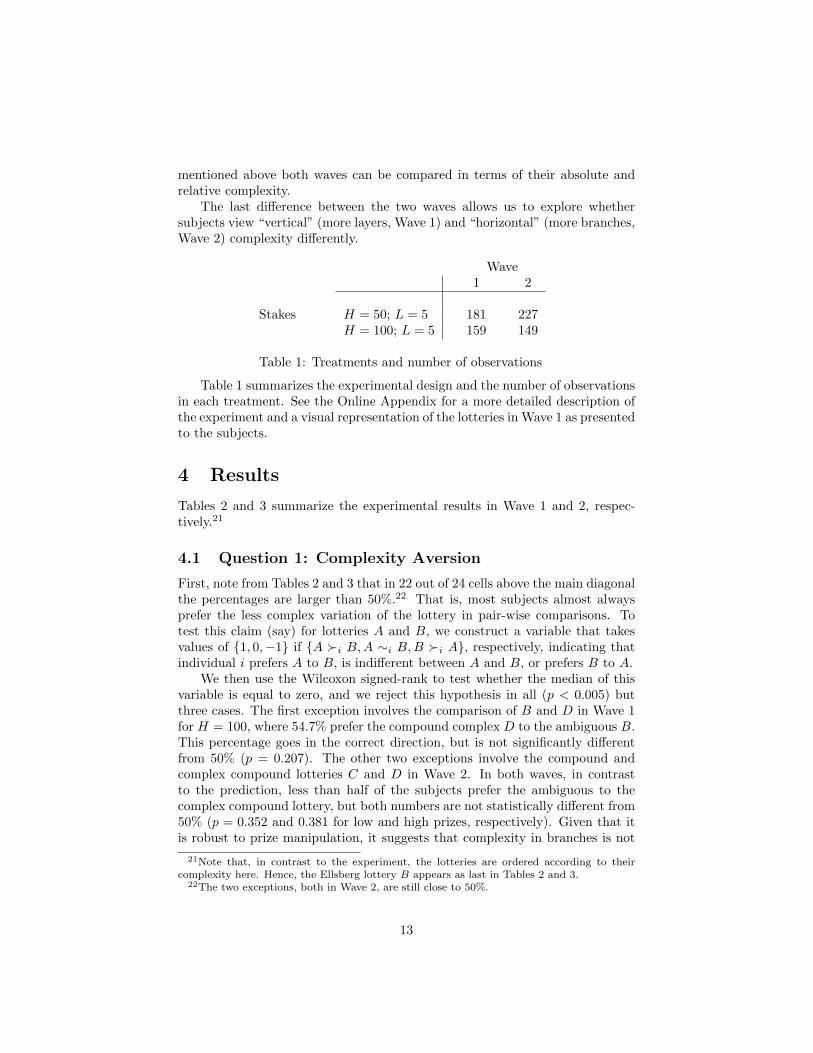
The last difference between the two waves allows us to explore whethersubjects view “vertical” (more layers, Wave 1) and “horizontal” (more branches,Wave 2) complexity differently.

Wave1 2

Stakes H = 50; L = 5 181 227H = 100; L = 5 159 149

Table 1: Treatments and number of observations

Table 1 summarizes the experimental design and the number of observationsin each treatment. See the Online Appendix for a more detailed description ofthe experiment and a visual representation of the lotteries in Wave 1 as presentedto the subjects.

4 Results

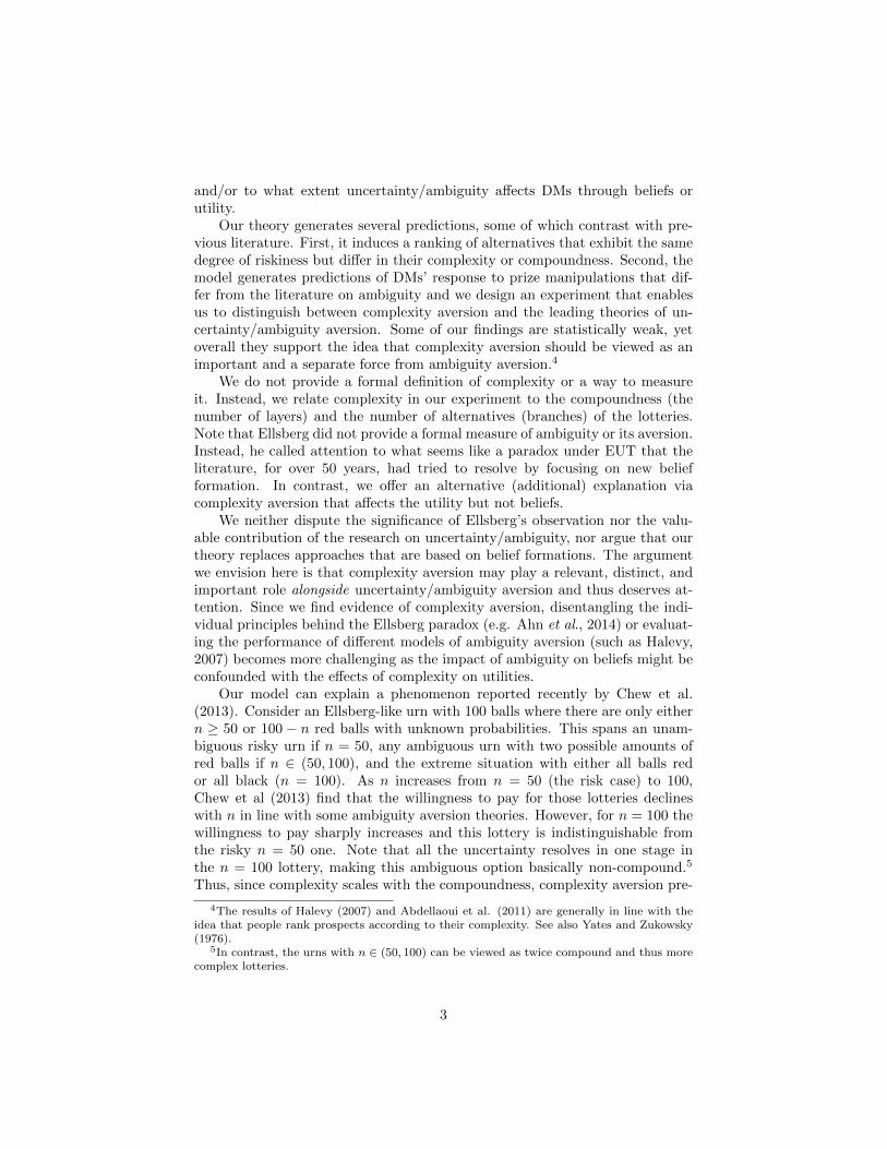
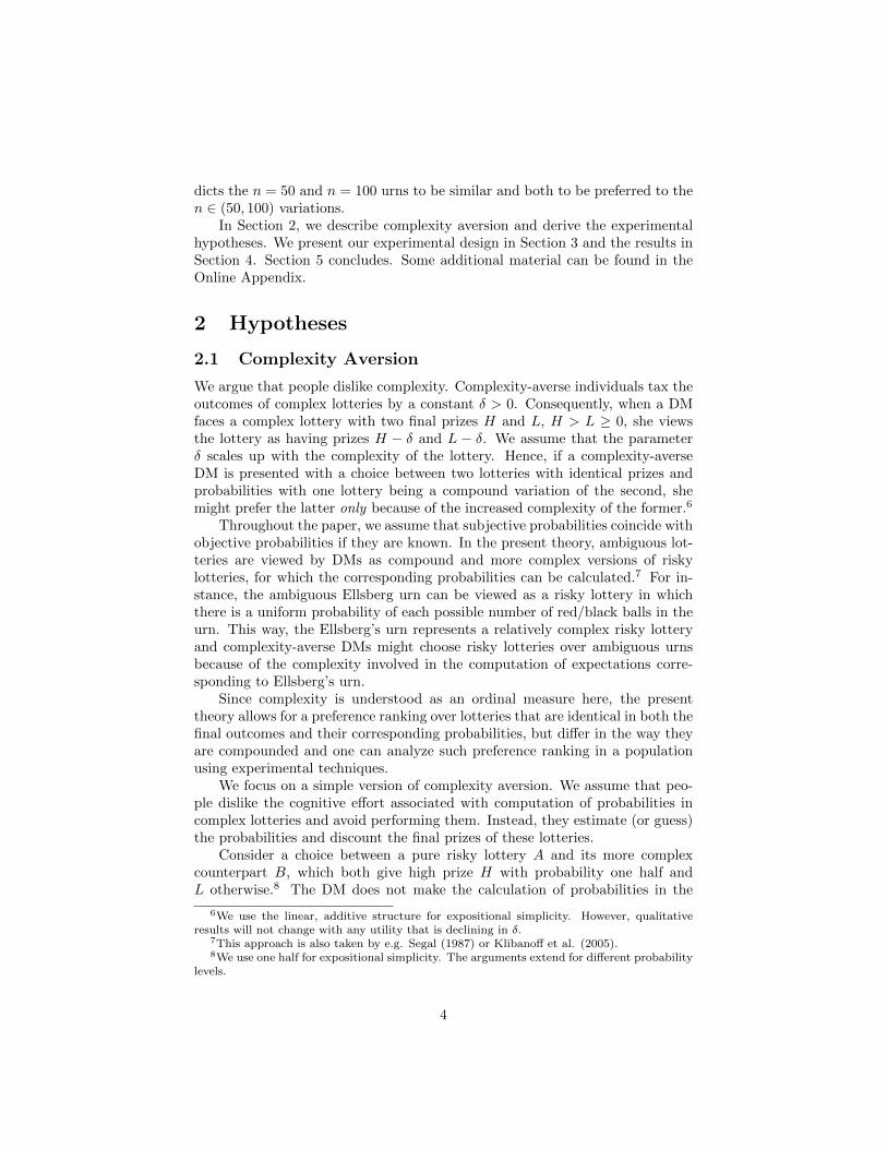
Tables 2 and 3 summarize the experimental results in Wave 1 and 2, respec-tively.21

4.1 Question 1: Complexity Aversion

First, note from Tables 2 and 3 that in 22 out of 24 cells above the main diagonalthe percentages are larger than 50%.22 That is, most subjects almost alwaysprefer the less complex variation of the lottery in pair-wise comparisons. Totest this claim (say) for lotteries A and B, we construct a variable that takesvalues of {1, 0,−1} if {A �i B,A ∼i B,B �i A}, respectively, indicating thatindividual i prefers A to B, is indifferent between A and B, or prefers B to A.

We then use the Wilcoxon signed-rank to test whether the median of thisvariable is equal to zero, and we reject this hypothesis in all (p < 0.005) butthree cases. The first exception involves the comparison of B and D in Wave 1for H = 100, where 54.7% prefer the compound complex D to the ambiguous B.This percentage goes in the correct direction, but is not significantly differentfrom 50% (p = 0.207). The other two exceptions involve the compound andcomplex compound lotteries C and D in Wave 2. In both waves, in contrastto the prediction, less than half of the subjects prefer the ambiguous to thecomplex compound lottery, but both numbers are not statistically different from50% (p = 0.352 and 0.381 for low and high prizes, respectively). Given that itis robust to prize manipulation, it suggests that complexity in branches is not

21Note that, in contrast to the experiment, the lotteries are ordered according to theircomplexity here. Hence, the Ellsberg lottery B appears as last in Tables 2 and 3.

22The two exceptions, both in Wave 2, are still close to 50%.

13

perceived as a sufficient complication to induce a ranking between these twooptions.

H = 50 (N = 181)

A: RiskC: Once

Compound

D: Twice

CompoundB: Ellsberg

A: Risk70.4%

(127.5)

72.7%

(131.5)

80.7%

(146)

C: Once

Compound

29.6%

(53.5)

61.6%

(111.5)

71.3%

(129)

D: Twice

Compound

27.3%

(49.5)

38.4%

(69.5)

60.8%

(110)

B: Ellsberg19.3%

(35)

28.7%

(52)

39.2%

(71)

H = 100 (N = 159)

A: RiskC: Once

Compound

D: Twice

CompoundB: Ellsberg

A: Risk71.4%

(113.5)

70.8%

(112.5)

81.4%

(129.5)

C: Once

Compound

28.6%

(45.5)

64.8%

(103)

67.9%

(108)

D: Twice

Compound

29.2%

(46.5)

35.2%

(56)

54.7%

(87)

B: Ellsberg18.6%

(29.5)

32.1%

(51)

45.3%

(72)

Note: If A ∼ B, then we count 0.5 observations for each, A and B, not

to lose these data. Hence, the decimals in paretheses.

Table 2. Lottery pairwise ranking: Wave 1. The percentage(number) in each cell is the percentage (number) of subjects

who prefer the row over the column lottery.

In addition and consistent with our model, there always exists an impor-tant fraction of individuals that still prefer the more complex–be it compoundor ambiguous–variation of each lottery.23 The exact numbers vary across treat-ments. In both waves, around 20% prefer the ambiguous to the risky lotteries.

23Wilcoxon signed-rank test rejects that the percentages are significantly different from zeroin all cases (p = 0 in all cases).

14

4.2 Question 2: Degree of Complexity

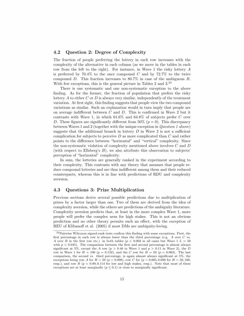
The fraction of people preferring the lottery in each row increases with thecomplexity of the alternative in each column (as we move in the tables in eachrow from the left to the right). For instance, in Wave 1 the risky lottery Ais preferred by 70.4% to the once compound C and by 72.7% to the twicecompound D. This fraction increases to 80.7% in case of the ambiguous B.With few exceptions, this is the general picture in Tables 2 and 3.24

There is one systematic and one non-systematic exception to the abovefinding. As for the former, the fraction of population that prefers the riskylottery A to either C or D is always very similar, independently of the treatmentvariation. At first sight, this finding suggests that people view the two compoundvariations as similar. Such an explanation would in turn imply that people areon average indifferent between C and D. This is confirmed in Wave 2 but itcontrasts with Wave 1, in which 61.6% and 64.8% of subjects prefer C overD. These figures are significantly different from 50% (p = 0). This discrepancybetween Waves 1 and 2 (together with the unique exception in Question 1 above)suggests that the additional branch in lottery D in Wave 2 is not a sufficientcomplication for subjects to perceive D as more complicated than C and ratherpoints to the difference between “horizontal” and “vertical” complexity. Sincethe non-systematic violation of complexity mentioned above involves C and D(with respect to Ellsberg’s B), we also attribute this observation to subjects’perception of “horizontal” complexity.

In sum, the lotteries are generally ranked in the experiment according totheir complexity. This contrasts with any theory that assumes that people re-duce compound lotteries and are thus indifferent among them and their reducedcounterparts, whereas this is in line with predictions of RDU and complexityaversion.

4.3 Questions 3: Prize Multiplication

Previous sections derive several possible predictions due to multiplication ofprizes by a factor larger than one. Two of them are derived from the idea ofcomplexity aversion, while the others are predictions of the ambiguity literature.Complexity aversion predicts that, at least in the more complex Wave 1, morepeople will prefer the complex urns for high stakes. This is not an obviousprediction and no other theory permits such an effect, with the exception ofREU of Klibanoff et al. (2005) if most DMs are ambiguity-loving.

24Pairwise Wilcoxon signed-rank tests confirm this finding with some exceptions. First, thefirst percentage in each row is always lower than the third percentage (e.g. A over C vs.A over B in the first row etc.) in both tables (p < 0.002 in all cases but Wave 1 L = 50with p < 0.045). The comparison between the first and second percentage is almost alwayssignificant at 5%, except the A row (p > 0.46 in Wave 1 and p > 0.11 in Wave 2), the Drow in Wave 1 for H = 100 (p = 0.132), and the C row for H = 50 (p = 0.063). The lastcomparison, the second vs. third percentage, is again almost always significant at 5%, theexceptions being row A for H = 50 (p = 0.098), row C for (p = 0.065, 0.698 for H = 50, 100,resp.), and row B (p = 0.99, 0.114 for low and high stakes, resp.). Note that most of theseexceptions are at least marginally (p ≤ 0.1) or close to marginally significant.

15

A quick look at the results of the treatment effects in Tables 2 and 3 suggeststhe following tendency: more people prefer more complex lotteries in Wave 1with higher stakes, while the contrary occurs in Wave 2 where complexity isminimized. This observation is consistent with complexity aversion and is atodds with theories that predict either no effect on the ranking or fewer peoplealways preferring the ambiguous lottery B after the prize manipulation. Theevidence here is weaker in the former case than in the latter though. However,most of the violations of our model again involve the lotteries C or D or both.

The general picture notwithstanding, with one exception, none of the dif-ferences across the stake variations in any cell are statistically significant at5% using the non-parametric Wilcoxon-Mann-Whitney rank sum test. In Wave1, the fraction of people preferring Ellsberg’s lottery B for H = 100 increasesby 3.4% (p = 0.504) in comparison with C and 6.1% in comparison with D(p = 0.236). The preference is roughly the same in the risky vs. Ellsbergcomparison (−0.7%; p = 0.82). The comparison of the risky and twice com-pound lotteries goes in the predicted direction (+1.9%; p = 0.7), while the Cvs. D comparison does not (−3.2%; p = 0.5). The two remaining cases provideroughly the same ranking in both stake variations (p > 0.82). The picture isclearer in Wave 2, but still statistically weak: fewer people always prefer themore complex lottery after the prize multiplication. Such a treatment effect isonly significant in the comparison of the risky and Ellsberg urn (p = 0.019), andvery marginally significant in the A vs. C (p = 0.148) and B vs. C comparisons(p = 0.128). The differences are small in the C vs. D (0.2%) and B vs. D (1%)cases.

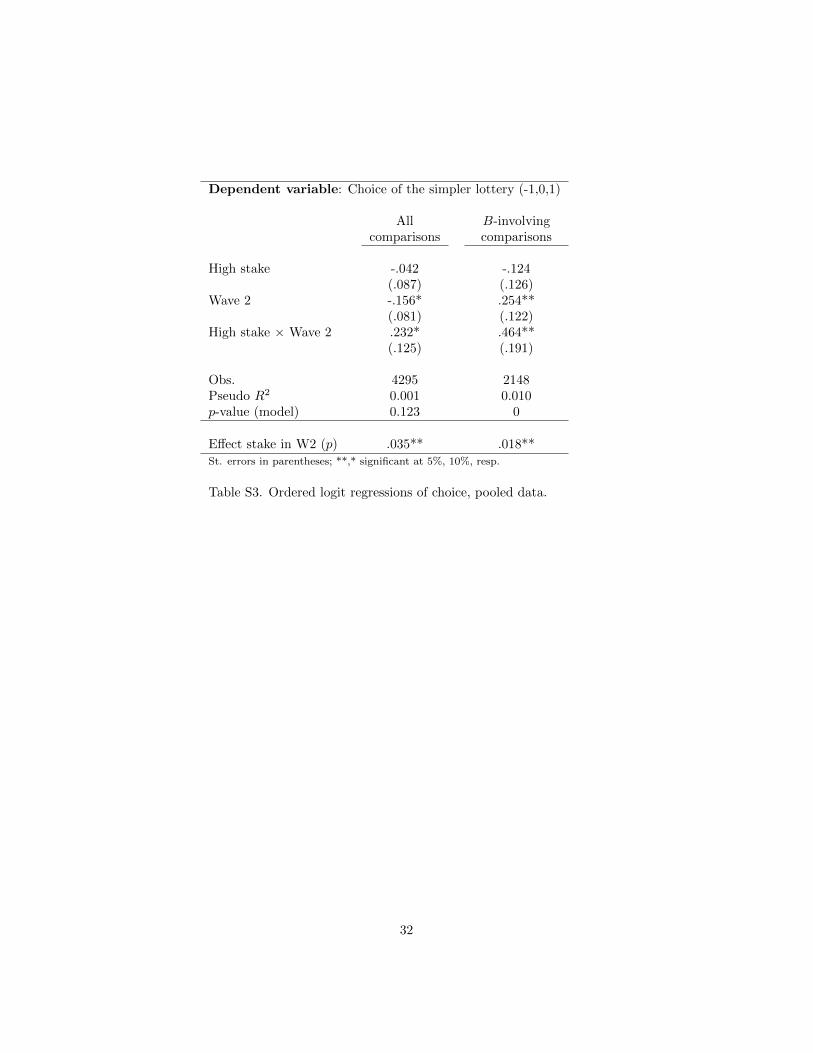
To move beyond these pairwise comparisons, we test the overall tendencyto prefer more complex lotteries if stakes are high in Wave 1 and the contraryeffect in Wave 2. To this aim, we pool the data from all the pairwise lotterycomparisons and all the treatments, and regress the choice of the simpler lotteryon a dummy for high stakes and Wave 2 and their interaction.25 This approachallows the testing of whether the treatment effects are significant but also servesto test whether the treatment effect is different across the two waves. This isimportant because ambiguity aversion predicts that it should not change fromone wave to the other, whereas complexity aversion predicts different reactionsto the stake manipulations across the two waves (see Question 3 ). We reporttwo regressions in Table S3 in the Online Appendix, one that contains all thepairwise lottery comparisons and one that only considers the comparisons thatinvolve the ambiguous lotteries B.

25Since the dependent variable takes values -1, 0, and 1 if, respectively, the individual prefersthe more complex lottery, she is indifferent between them, or she prefers the simpler option, weestimate the ordered-logit model. The results are generally robust to alternative specificationsof the dependent variable, different estimation techniques, or panel data regressions, in whichsubjects’ different choices play the role of the time-series variable.

16

H = 50 (N = 227)

A: Risk C: CompoundD: Complex

CompoundB: Ellsberg

A: Risk59.5%

(135)

61.7%

(140)

79.7%

(181)

C: Compound40.5%

(92)

46.9%

(106.5)

73.1%

(166)

D: Complex

Compound

38.3%

(87)

53.5%

(120.5)

71.6%

(162.5)

B: Ellsberg20.3%

(46)

26.9%

(61)

28.4%

(64.5)

H = 100 (N = 149)

A: Risk C: CompoundD: Complex

CompoundB: Ellsberg

A: Risk66.1%

(98.5)

61.1%

(91)

88.6%

(132)

C: Compound33.9%

(50.5)

46.6%

(69.5)

79.9%

(119)

D: Complex

Compound

38.9%

(58)

53.4%

(79.5)

74.5%

(111)

B: Ellsberg11.4%

(17)

20.1%

(30)

25.5%

(38)

Note: If A ∼ B, then we count 0.5 observations for each, A and B, not

to lose these data. Hence, the decimals in parentheses.

Table 3. Lottery pairwise ranking: Wave 2. The percentage(number) in each cell is the percentage (number) of subjects

who prefer the row over the column lottery.

The regressions corroborate that people increase their preference for morecomplex lotteries after the prize multiplication in Wave 1, whereas the contraryoccurs in Wave 2. Once again, this effect is statistically weak in Wave 1 but theoverall effect is significant in Wave 2 (p = 0.035 and 0.018 if all comparisons oronly B-involving comparisons are considered, respectively).

Most importantly, the treatment effects differ across the two waves (p =0.064 and 0.015, respectively). This points to a non-trivial interaction betweencomplexity and ambiguity, contrasting the belief-models of ambiguity aversion

17

and supporting our complexity aversion. The support for our theory is gener-ally stronger if only B-involving comparisons are considered (compared to theregression considering all the comparisons; see Table S3 in Online Appendix C).We suspect that this may be due to the problematic comparisons between Cand D.

To conclude, complexity aversion that takes into account the effect of prizemanipulation on the distribution of estimated probabilities of lottery prizes isthe best predictor of the qualitative shift of preferences observed in the lab. Eventhough statistically weak, the treatment effects move in the predicted direction.Moreover, we find strong evidence for different impact of our payoff manipu-lation across the two waves, pointing to an interaction between ambiguity andcomplexity.26

5 Conclusions

We propose a simple alternative (and/or additional) resolution to the Ellsbergparadox. Ours focuses on aversion to complexity, presented here as compound-ness, affecting utility but otherwise consistent with EUT, rather than the typi-cal resolutions based on new structures of beliefs. Complexity-averse decision-makers regard complexity as disutility and thus less valued than a similar butless complex lottery. Our simple model allows the existence of a priori in Ells-berg’s ambiguous urn, making a choice under risk but with compound lotteries.We demonstrate that the Ellsberg paradox can be explained by complexity aver-sion even if we abstract from ambiguity aversion. Our experimental results arein most respects consistent with complexity aversion and with previous evidence(e.g. Halevy (2007)). In particular, subjects exhibit a preference ranking overlotteries that reflects their degree of complexity and the impact of payoff ma-nipulation seems to interact with the general complexity of our experimentallotteries.

Recognizing possible interactions between ambiguity and complexity, wedesign our experiment to illustrate that complexity aversion plays a separaterole from ambiguity aversion. When we move to an overall more simple scenario(from Wave 1 to Wave 2), we do not see an increase in the number of subjectspreferring the risky A over the ambiguous B. When we multiply prizes butkeep complexity the same, the observed effects can be explained by complexityaversion theory, whereas ambiguity aversion is mostly silent on that.

26In his experiment, Halevy (2007) provides a robustness test of his main treatment, inwhich he multiplies the stakes by 10. We used his data and found that 22.2% prefer theEllsberg-like lottery to the risky one for low stakes, but this fraction increases to 25% if stakesare higher. The difference is not statistically significant, though. There are three reasons whythis additional finding may support complexity aversion: (i) any increase already contradictsmost of the theories of ambiguity aversion, (ii) there are only 38 observations in the high-stake treatment, (iii) multiplying the stakes by 10 should increase subjects’ estimation effortconsiderably and thus work against the prediction of complexity aversion. In contrast, histen-ball lotteries are more complex than ours. Hence, we consider his data stimulating forfurther exploration of complexity aversion but prefer to be cautious using this data to makegeneral conclusions concerning our theory.

18

This evidence points out that the future literature should take into accountthat people are likely to be averse to complexity vis-a-vis utilities and not just toambiguity due to unknown probabilities, and that complexity aversion (e.g. asmodeled here) can affect decisions and behavior in a different way. Complexityaversion may play a complementary role alongside risk and ambiguity aversion.Obviously, complexity (as separate from ambiguity) aversion should be furtherstudied in the laboratory and in the field to understand it better.

References

[1] Abdellaoui, M., P. Klibanoff, and L. Placido (2011): Ambiguity and Com-pound Risk Attitudes: An Experiment, mimeo, HEC Paris.

[2] Ahn, D., Choi, S., Gale, D., & Kariv, S. (2014). Estimating ambiguityaversion in a portfolio choice experiment, Quantitative Economics 5, 195-223.

[3] Anscombe, F. J., and R. J. Aumann (1963): “A Definition of SubjectiveProbability,” The Annals of Mathematical Statistics 34, 199–205.

[4] Chew, S.H., B. Miao, and S. Zhong (2013): Partial Ambiguity, mimeo,National University of Singapore.

[5] Ergin, H. and F. Gul (2009): “A Theory of Subjective Compound Lotter-ies,” Journal of Economic Theory 144, 899-929.

[6] Ellsberg, D. (1961): “Risk, Ambiguity and the Savage Axioms,” The Quar-terly Journal of Economics 75, 643–669.

[7] Ghirardato, P., F. Maccheroni, and M. Marinacci (2004): “DifferentiatingAmbiguity and Ambiguity Attitude.” Journal of Economic Theory 118,133–73.

[8] Gilboa, I. and M. Marinacci (2013), “Ambiguity and the BayesianParadigm”, Advances in Economics and Econometrics: Theory and Appli-cations, Tenth World Congress of the Econometric Society. D. Acemoglu,M. Arellano, and E. Dekel (Eds.). New York: Cambridge University Press.

[9] Gilboa, I. and D. Schmeidler (1989), Maxmin expected utility with a non-unique prior. Journal of Mathematical Economics, 18, 141-153.

[10] Grant, S., B. Polak, and T. Strzalecki (2009), Second-order expected utility,mimeo, Harvard University.

[11] Halevy, Y. (2007), Ellsberg Revisited: An Experimental Study. Economet-rica, 75, 503-536.

[12] Hill, B. (2011): Confidence and Decision, mimeo, HEC Paris(http://www.hec.fr/hill).

19

[13] Klibanoff, P., M. Marinacci, and S. Mukerji (2005), A smooth model ofdecision making under ambiguity. Econometrica, 73, 1849-1892.

[14] Quiggin, J. (1982): “A Theory of Anticipated Utility,” Journal of EconomicBehavior and Organization 3, 323–343.

[15] Maccheroni, F., M. Marinacci and A. Rustichini (2006): “AmbiguityAversion, Robustness, and the Variational Representation of Preferences,”Econometrica 74, 1447-1498.

[16] Savage, L. J. (1954): The Foundations of Statistics. New York: Wiley.

[17] Schmeidler, D. (1989): Subjective Probability and Expected Utility With-out Additivity, Econometrica 57, 571–587.

[18] Segal, U. (1987), The Ellsberg Paradox and Risk Aversion: An AnticipatedUtility Approach. International Economic Review 28, 175-202.

[19] Segal, U. (1990), Two-stage lotteries without the reduction axiom. Econo-metrica 58, 349-377.

[20] Yates, F.J. and L.G. Zukowski (1976), “Characterization of Ambiguity inDecision Making,” Behavioral Science 21, 19–25.

20

Appendix A

Let there be a strictly increasing (and concave) von Neuman-Morgenstern util-ity function u(.), with u(0) = 0, and assume that subjective probabilities arereplaced by the objective ones if the former are known.

A.1 Question 1: Complexity aversion

Most of the models focus on how DMs form their beliefs about the probabilitiesof individual outcomes. With two outcomes, H and L in our example, all thesetheories say that B � A by a DM if

γu(H) + (1− γ)u(L) ≥ 12u(H) + 1

2u(L)⇔ [u(H)− u(L)](γ − 12 ) ≥ 0. (2)

In words, if γ ≥ 12 , DMs prefer B to A. That is, all these models allow people

to choose the ambiguous B if γ is high enough. This holds for subjective ex-pected utility (SEU), Choquet expected utility (CEU), maximin expected utility(MMEU), and α−maximin model (α−MEU).

Under SEU (e.g. Savage, 1957, or Anscombe and Aumann, 1963), DMschoose the complex lottery B over A if their belief about the probability ofhigh prize in B is higher than one half. With two options, the CEU modelof Schmeidler (1989) makes the same prediction. The subjective probability isreplaced by a “capacity” measure υ(.) that does not have to add up to one toreflect the degree of beliefs in the probabilities of the prizes of a lottery. Again,if υ(H) is high enough, the subject might prefer lottery B. In MMEU, Gilboaand Schmeidler (1989) propose to replace the capacities by the most pessimisticpriors (in terms of expected utilities), while the α−MMEU (Ghirardato et al.,2004) argues in favour of a convex combination of the most pessimistic and themost optimistic beliefs. If these priors are biased toward high probabilities ofH, B can be preferred to A.

The rank-dependent utility or RDU (Segal, 1987, 1990) incorporates therank-dependent utility model of Quiggin (1982). In this theory, it is assumedthat DMs view ambiguous lotteries as compounded variations of reduced lot-teries for which corresponding probabilities can be computed, but they do notreduce them correctly. More precisely, DMs see the Ellsberg urn as a two stagelottery. The first stage corresponds to the probabilities of chosen ball selectiongiven the urn composition, while the second stage refers to the probabilities overthe possible states of nature (e.g. the possible 101 compositions of the originalEllsberg urn). Which lottery is then selected depends on the beliefs about thelikelihood of the high prize in both the ambiguous and risky lotteries.

To simplify matters, consider a ten-ball variations of the original Ellsbergurns. In RDU, outcomes are ranked and probabilities are weighted by an in-creasing function f : [0, 1] → [0, 1], satisfying f(0) = 0 and f(1) = 1. Letβi ∈ [0, 1] denote the DM’s belief that the urn contains i balls of the color the

DM bets on; i = 0, 1, 2, ..., 10 and∑10

i=0 βi = 1. DMs first compute the expectedRDU for each possible situation in the second stage and the corresponding cer-tainty equivalents of each alternative are used to compute the final weights in

21

the first-stage lottery. Consequently, the DM prefers the ambiguous to the riskylottery if

γu(H) + (1− γ)u(L) ≥ f( 12 )u(H) + [1− f( 1

2 )]u(L), (3)

where γ ={∑10

i=1 f(∑10

j=i βi)[f(∑i

j=0j10 )− f(

∑i−1j=0

j10 )]}

. We can see that,

depending on the priors about the composition of the ambiguous urn and theshape of the weighting function f(.), the RDU DMs will prefer one or the otheroption. For example, if the DM believes that the ambiguous urn contains 10 redballs with probability one (i.e. β10 = 1 and βi = 0 for i = 0, 1, ..., 9), the left-hand side of (3) reduces to u(H) and she bets on red and selects the ambiguousurn. If, instead, the DM has a uniform prior about the second-stage lottery,Theorem 4.2 in Segal (1987) establishes several conditions on f(.) such that theDM behaves as ambiguity averse, i.e. she is indifferent between the two colorsbut selects the risky urn.

As in RDU, Klibanoff et al. (2005) assume that people see ambiguouslotteries as two-stage probability draws and propose a theory labeled as recursiveexpected utility (REU) by Halevy (2007). The REU from choosing the ten-ballvariation of Ellsberg’s lottery (labeled B here) has the following form:

UREU (B) =

10∑j=i

βiφ

[i

11u(H) +

11− i11

u(L)

].

The von Neuman-Morgenstern u(.) determines the risk aversion of DMs, whilethe attitudes toward ambiguity are captured by the function φ. The choice of aDM between the risky and ambiguous lotteries will be driven by the shape of φ:if φ is concave (convex) the DM is ambiguity averse (loving).27 In our simpleexample with two options, A � B if and only if

12u(H) + 1

2u(L) ≥ βφ[u(H)] + (1− β)φ[u(L)]. (4)

Hence, people may reject the ambiguous B for two reasons. Either they areambiguity-averse (reflected by φ) and/or their belief about H is low enough.

Last, variational preferences (VP) of Maccheroni et al. (2006) take intoaccount the possibility that DMs are well aware that their beliefs might not becorrect. They axiomatize a model such that the expected utility from lotteriesand actions with unknown probabilities accounts for such uncertainty, using afunction c(p). This function reflects the degree of uncertainty about subjectiveprobabilities described by p and can be viewed as a measure of distance betweenthe priors considered, p, and the best guess of the DM. In risky lotteries, wecan set c(p) = ∞ for any p different from the objective probabilities and these

27There exist a class of models known as source dependent or second-order expected utilitywhich can be thought of as a special case of REU (e.g. Ergin and Gul (2009), Grant et al.(2009)). In this approach, people reduce compound lotteries but view risk and uncertaintydifferently. For these reasons, we do not discuss this approach in more detail here and focuson REU.

22

possible priors are never relevant for the decision. Formally,28

UV P (A) = 12u(H) + 1

2u(L) ≥ minp∈4(S)

[pu(H) + (1− p)u(L) + c(p)] = UV P (B).

(5)Hence, people who believe that balls of a certain color are highly present in theambiguous urn and put high enough confidence in these beliefs might choosethis color and select B over the risky A.

A.2 Question 2: Degree of complexity

Since all the one-stage theories of ambiguity aversion assume that people re-duce compound lotteries when information is provided objectively, they predictthat subjects should be indifferent among the compound variations of the samerisky lottery.29 This also holds for the two-stage REU, since if probabilities areobjective φ(.) does not apply. Nevertheless, we observe a systematic ranking ac-cording to the “degree of complexity” in the experiment even if the probabilitiesare objective.

The only exception is the two-stage RDU, since both the compound andambiguous options are viewed as compound lotteries independently of whetherthe probabilities are objective or subjective. In particular, if the conditions onf(.) corresponding to ambiguity aversion hold, people may rank a risky lotteryover its once compound payoff-equivalent variation, the latter over the twicecompound variation and so on. Let us illustrate this on the lotteries from Wave1.30 Denote Wj the bet on white in lottery j ∈ {A,B,C,D}. Then,

URDU (WA) = u(L) + [u(H)− u(L)]f(0.5).

In the once compound lottery C, a RDU DM first evaluates the second-stage sublotteries SL2

left = (H, 0.5;L, 0.5), and SL2right = (H, 0.75;L, 0.25) as

follows: URDU (WSL2left) = u(L) + [u(H)−u(L)]f(0.5) and URDU (WSL2

left) =u(L) + [u(H)− u(L)]f(0.75).

Since URDU (WSL2right) > URDU (WSL2

left),

URDU (WC) = u{u−1

[URDU (WSL2

left)]}

+

+(u{u−1

[URDU (WSL2

right)]}− u

{u−1

[URDU (WSL2

left)]})

f(0.5)

= u(L) + [u(H)− u(L)] f(0.5) [1 + f(0.75)− f(0.5)]

Then, URDU (WA) > URDU (WC) if and only if

f(5/8)

f(0.5)> 1 + f(0.75)− f(0.5).

28S can be considered the set of subjective beliefs about the possible states of the world.29In VP, c(p) =∞ for any p different from the objective probabilities in VP. The function

c(.) thus plays no role in risky and compound lotteries.30The intuitions extend to Wave 2.

23

In a similar vein, we can compute URDU (WD) and show that, under certainconditions on f(.) characterized in Theorem 4.2 in Segal (1987), RDU DM canexhibit the following ranking: URDU (WA) > URDU (WC) > URDU (WD) >URDU (WB) if she holds, for instance, uniform priors in B. Hence, this is theonly model that can generate the same prediction as our complexity aversion,while all other theories of aversion to ambiguity predict indifference betweenrisky and their payoff-equivalent compound variations.

A.3 Question 3: Prize Multiplication and Ambiguity Liter-ature

What do the belief-based explanations of the Ellsberg paradox predict whenlottery prizes are multiplied by two? To answer this question, note first that(i) if the probabilities are the same before and after the prize multiplication thepriors should not be affected by such payoff manipulation, and (ii) the expression(2) is satisfied if and only if

γu(2H)+(1−γ)u(2L) ≥ 12u(2H)+ 1

2u(2L)⇔ [u(2H)−u(2L)](γ− 12 ) ≥ 0. (6)

That is, as well as in (2), DMs prefer B to A if and only if γ ≥ 12 . As a result, the

theories that can be characterized by (2) may differ in the weight γ and, thus,generate different predictions about the number of people preferring one optionto the other. However, they all agree that the number of people preferring eachoption should not change before and after the prize multiplication, since theweights γ from (2) and (6) are the same and compare to 1

2 in these theories.This is true for SEU, CEU31, MMEU, and α−MEU.

This intuition also extends to RDU. Hence, even though RDU and com-plexity aversion cannot be separated on basis of Question 2, they generate adifferent hypothesis regarding the prize multiplication.

The REU model of Klibanoff et al. (2005) provides no general predictionabout the effect of prize multiplication. If we focus on ambiguity-averse REU(that is, a concave φ), the concavity implies that if (4) holds

12u(2H) + 1

2u(2L) ≥ βφ[u(2H)] + (1− β)φ[u(2L)].

In words, ambiguity-averse subjects who choose the risky option for low stakesshould also do so in the high-stakes treatment. Only B-choosing ambiguity-averse individuals may switch their choice to A for high stakes. However, thecontrary holds for risk seeking individuals. Consequently, the effect depends onthe distribution of shapes of φ in the population. If we expect the majority ofour subjects to be ambiguity-averse as typically observed in experiments, REUwould predict more ambiguity aversion-like behavior after the prize manipula-tion.

One more conservative implication of REU is that we can observe more,fewer or the same number of people preferring the ambiguous lotteries over

31Formally, [u(H)− u(L)](v(H)− 12

) ≥ 0 if and only if [u(2H)− u(2L)](v(H)− 12

) ≥ 0.

24

risky ones after the prize multiplication. Apart from aversion to complexity,this is the only theory that permits more people preferring B after the prizesincrease. However, this prediction does not depend on any other feature ofthe experiment; the effect only depends on the distribution of preferences inthe population. As a result, REU predicts the same effect (whatever it is),independently of the general complexity of experimental lotteries in each wave.In contrast, complexity aversion predicts an interplay between complexity andambiguity across the two waves.

Finally, VP of Maccheroni et al. (2006) make the same prediction as REUunder convex φ. Formally, since c(.) is independent of the stakes, it generatesan interplay between stakes and the impact of the confidence in own subjectiveprobabilities and (5) thus implies

UV P (A) = 12u(2H)+ 1

2u(2L) ≥ minp∈4(S)

[pu(2H) + (1− p)u(2L) + c(p)] = UV P (B).

Under VP, given that the function c(p) loses relative importance for higherstakes people that prefer the risky A before the multiplication will also prefer itafterwards. Hence, if someone changes her choice, she switches from the ambigu-ous B to A, but not vice versa. Consequently, VP predict that unambiguouslymore people will prefer the risky urn after our prize manipulation.32

A.4 Holding L fixed in prize manipulation

In the main exposition of complexity aversion, we multiply both prizes by thesame factor, but in the actual experiment we only double H, holding L fixed.Here, we show that all the results derived above extend to such a scenario. Thethreshold before the multiplication remains the same. If we double H (and holdL), B � A if and only if

θ(2H − δ) + (1− θ)(L− δ) > 1

2(2H + L)⇔ θ > θ =

1

2+

δ

2H − L.

It is easy to see that θ < θ∗. Hence, the threshold also falls in this case.The contrast of complexity aversion and the ambiguity literature also holds

under the current specification. Note that

γu(H) + (1− γ)u(L) ≥ 12u(H) + 1

2u(L)⇔ [u(H)− u(L)](γ − 12 ) ≥ 0 (7)

if and only if

γu(2H) + (1− γ)u(L) ≥ 12u(2H) + 1

2u(L)⇔ [u(2H)− u(L)](γ − 12 ) ≥ 0. (8)

32Last, the confidence model of Hill (2011) is directly based on the idea that stakes shouldinteract with how much confidence in their subjective beliefs DMs require in order to bet onoptions with unknown probabilities. In particular, he argues that the higher the stakes themore confident DMs should be. As a consequence, the model predicts that, ceteris paribus,fewer people should choose the ambiguous lotteries if prizes are multiplied.

25

As a consequence, SEU, CEU, MMEU and α−MEU predict no change after suchprize manipulation, and similar considerations apply to RDU. The predictionsfor REU are independent of the stakes in question, while the sensitivity of VPand Hill’s (2011) confidence model on stakes remains as long as at least one ofthe prizes increases.

In sum, all the predictions stated in the main text extend to the contextpresented to experimental subjects.

Appendix B: Experimental Instructions (Wave 1,low stakes)

Experiment of Lottery Preferences

Welcome to our study. This experiment is being conducted as a part of a re-search project on people’s preference. The whole session will last approximately15 minutes.

Instructions:

1. After we read the instructions and you understand the task, if you arewilling to participate, please print your name on the last page of thisquestionnaire (consent form), sign and date it.

2. Read the descriptions of four lotteries in the following pages. Try to under-stand how they operate and rank/order them according to your preference.Put down your preferences where asked in the questionnaire.

3. Hand in the questionnaire.

4. Wait for our announcement of those who are invited to participate in ourreal lotteries.

Rewards:After we have collected all the questionnaires, we will randomly pick several

out them (roughly 1/10 of the class size). Those whose questionnaires are drawnwill be invited to try their luck in an actual realization of the lotteries we havedevised for this study which are explained below.

We will pick two of the four lotteries and run the lottery, which you preferaccording to your answers in this questionnaire. You will be able to observe theresult instantly. You can then collect the prize money after just a little paperwork.

If you are one of the lucky ones, but prefer to do the actual lottery privately;please let us know and we can set up an appointment.

Caution:This is a serious experiment. Please avoid discussing, looking at others’

questionnaire or exclaiming. Should you have any questions please raise yourhand and we will be happy to assist you.

26

The lotteries:We have created four lotteries labeled A, B, C and D. Please follow our

description of each of them below and pay attention to our explanations. If youhave any questions about any of them, please do not hesitate to ask us.

All the information provided here is accurate to our knowledge and is in-tended to help you understand the mechanism of the lotteries. Any student whois invited to participate in our actual realization of the lotteries is welcome toverify that the provided information is true.

Lottery A: There is one non-transparent brown bag, with 8 chips in it. 5of these chips are white and the other 3 are black, as in figure A. You are askedto announce a color, white or black, at your own choice. Then a chip is drawnfrom the bag. You will be awarded $50 if the color of the chip matches the colorof your choice, and $5 otherwise.

Lottery B: There is one non-transparent brown bag with 6 chips in it, asin figure B. Each chip is either white or black, but you do not know the exactnumber of chips of either color. You are asked to announce a color, white orblack, at your own choice. 2 chips of that color are put in to the brown bag tomake it 8 chips in total. Then a chip is drawn from the brown bag. You willbe awarded $50 if the color of the chip matches the color of your choice, and $5otherwise.

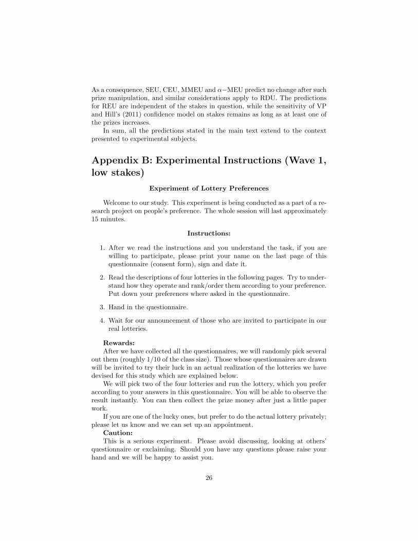
Lottery C: There are two non-transparent brown bags each with 4 chipsin it, as in figure C. The first bag contains 2 white chips and 2 black chips. Thesecond bag contains 3 white chips and 1 black chip. You are asked to announcea color, white or black, at your own choice. After that, we flip a fair coin. Ifit is heads we use the first bag, if tails, we use the second bag. Therefore, eachbag has equal chance to be selected. Then a chip is drawn from the chosen bag.You will be awarded $50 if the color of the chip matches the color of your choice,and $5 otherwise.

27

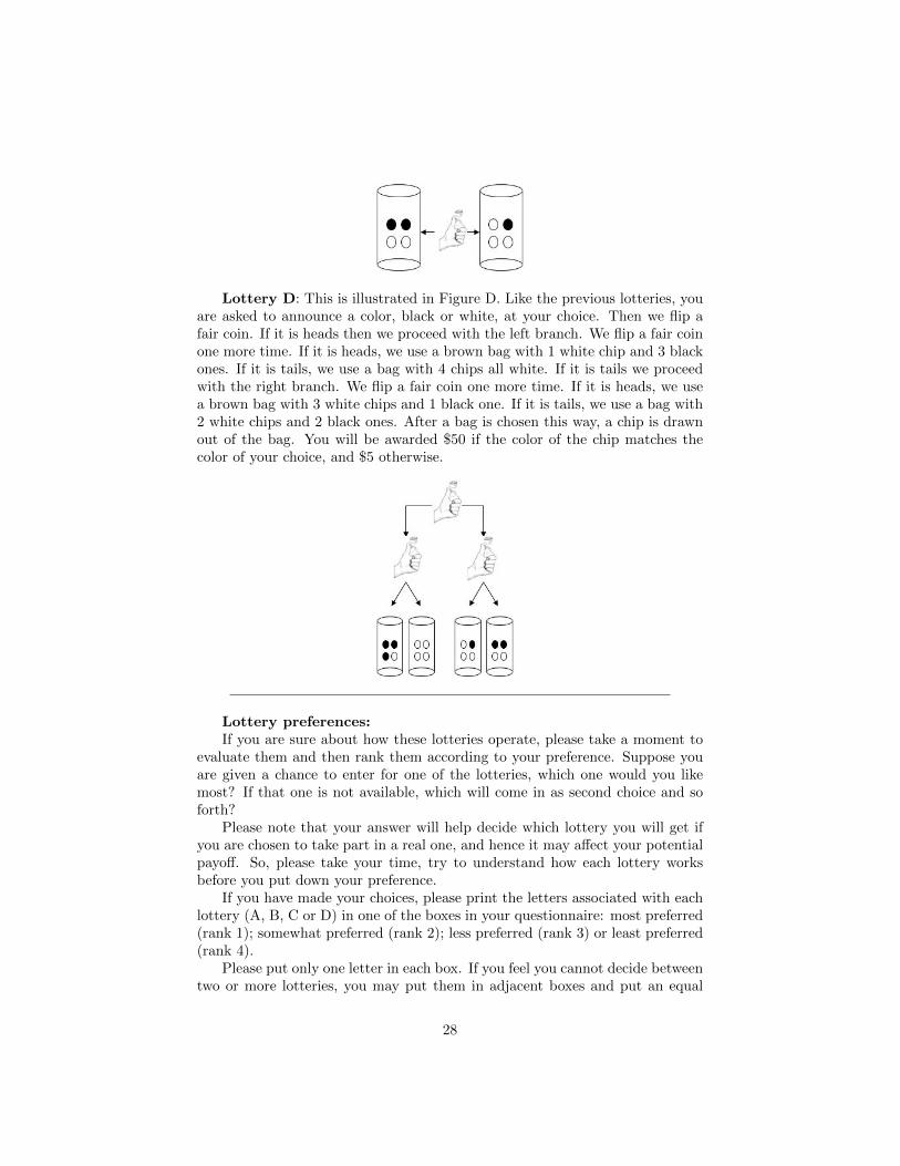
Lottery D: This is illustrated in Figure D. Like the previous lotteries, youare asked to announce a color, black or white, at your choice. Then we flip afair coin. If it is heads then we proceed with the left branch. We flip a fair coinone more time. If it is heads, we use a brown bag with 1 white chip and 3 blackones. If it is tails, we use a bag with 4 chips all white. If it is tails we proceedwith the right branch. We flip a fair coin one more time. If it is heads, we usea brown bag with 3 white chips and 1 black one. If it is tails, we use a bag with2 white chips and 2 black ones. After a bag is chosen this way, a chip is drawnout of the bag. You will be awarded $50 if the color of the chip matches thecolor of your choice, and $5 otherwise.

Lottery preferences:If you are sure about how these lotteries operate, please take a moment to

evaluate them and then rank them according to your preference. Suppose youare given a chance to enter for one of the lotteries, which one would you likemost? If that one is not available, which will come in as second choice and soforth?

Please note that your answer will help decide which lottery you will get ifyou are chosen to take part in a real one, and hence it may affect your potentialpayoff. So, please take your time, try to understand how each lottery worksbefore you put down your preference.

If you have made your choices, please print the letters associated with eachlottery (A, B, C or D) in one of the boxes in your questionnaire: most preferred(rank 1); somewhat preferred (rank 2); less preferred (rank 3) or least preferred(rank 4).

Please put only one letter in each box. If you feel you cannot decide betweentwo or more lotteries, you may put them in adjacent boxes and put an equal

28

sign “=” in between. However, if you are to be chosen to play in our realizedlottery and the two lotteries available deemed “equal” by you, we will pick onefor you to participate.

Most Preferred Somewhat Preferred Less Preferred Least Preferred

(Rank 1) (Rank 2) (Rank 3) (Rank 4)

Thanks for your participation. Please do not forget to sign the next page.

29

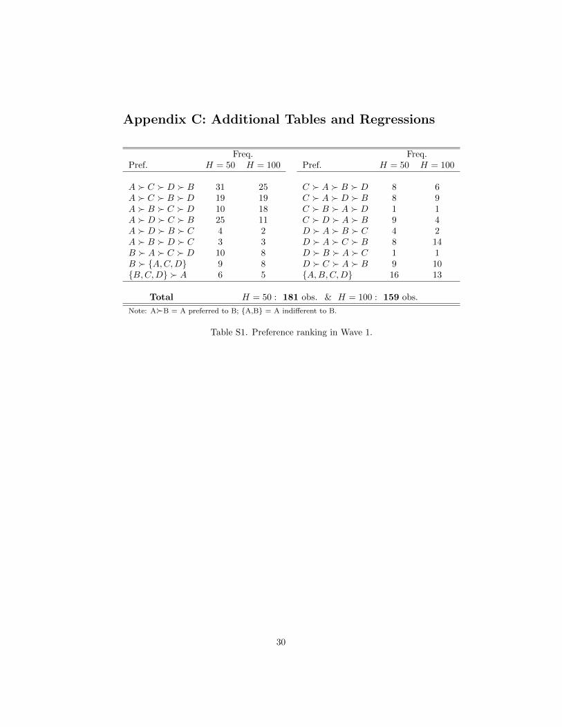
Appendix C: Additional Tables and Regressions

Freq. Freq.Pref. H = 50 H = 100 Pref. H = 50 H = 100

A � C � D � B 31 25 C � A � B � D 8 6A � C � B � D 19 19 C � A � D � B 8 9A � B � C � D 10 18 C � B � A � D 1 1A � D � C � B 25 11 C � D � A � B 9 4A � D � B � C 4 2 D � A � B � C 4 2A � B � D � C 3 3 D � A � C � B 8 14B � A � C � D 10 8 D � B � A � C 1 1B � {A,C,D} 9 8 D � C � A � B 9 10{B,C,D} � A 6 5 {A,B,C,D} 16 13

Total H = 50 : 181 obs. & H = 100 : 159 obs.

Note: A�B = A preferred to B; {A,B} = A indifferent to B.

Table S1. Preference ranking in Wave 1.

30

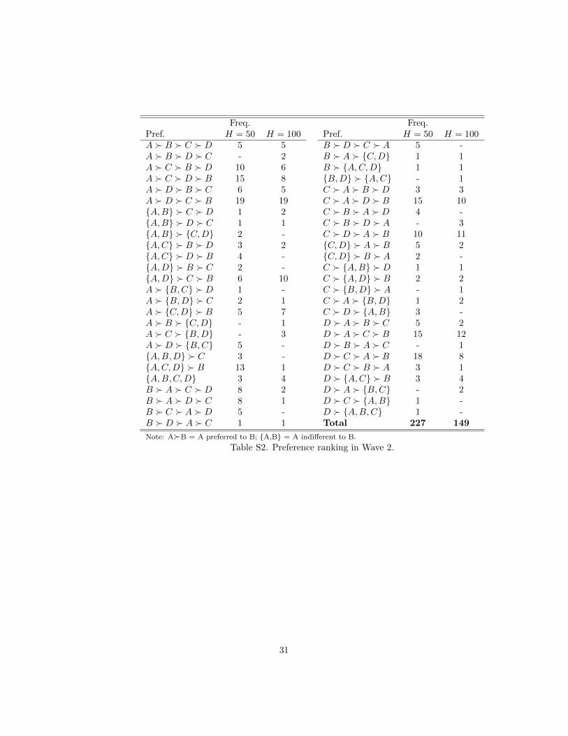
Freq. Freq.Pref. H = 50 H = 100 Pref. H = 50 H = 100A � B � C � D 5 5 B � D � C � A 5 -A � B � D � C - 2 B � A � {C,D} 1 1A � C � B � D 10 6 B � {A,C,D} 1 1A � C � D � B 15 8 {B,D} � {A,C} - 1A � D � B � C 6 5 C � A � B � D 3 3A � D � C � B 19 19 C � A � D � B 15 10{A,B} � C � D 1 2 C � B � A � D 4 -{A,B} � D � C 1 1 C � B � D � A - 3{A,B} � {C,D} 2 - C � D � A � B 10 11{A,C} � B � D 3 2 {C,D} � A � B 5 2{A,C} � D � B 4 - {C,D} � B � A 2 -{A,D} � B � C 2 - C � {A,B} � D 1 1{A,D} � C � B 6 10 C � {A,D} � B 2 2A � {B,C} � D 1 - C � {B,D} � A - 1A � {B,D} � C 2 1 C � A � {B,D} 1 2A � {C,D} � B 5 7 C � D � {A,B} 3 -A � B � {C,D} - 1 D � A � B � C 5 2A � C � {B,D} - 3 D � A � C � B 15 12A � D � {B,C} 5 - D � B � A � C - 1{A,B,D} � C 3 - D � C � A � B 18 8{A,C,D} � B 13 1 D � C � B � A 3 1{A,B,C,D} 3 4 D � {A,C} � B 3 4B � A � C � D 8 2 D � A � {B,C} - 2B � A � D � C 8 1 D � C � {A,B} 1 -B � C � A � D 5 - D � {A,B,C} 1 -B � D � A � C 1 1 Total 227 149

Note: A�B = A preferred to B; {A,B} = A indifferent to B.

Table S2. Preference ranking in Wave 2.

31

Dependent variable: Choice of the simpler lottery (-1,0,1)

All B-involvingcomparisons comparisons

High stake -.042 -.124(.087) (.126)

Wave 2 -.156* .254**(.081) (.122)

High stake × Wave 2 .232* .464**(.125) (.191)

Obs. 4295 2148Pseudo R2 0.001 0.010p-value (model) 0.123 0

Effect stake in W2 (p) .035** .018**St. errors in parentheses; **,* significant at 5%, 10%, resp.

Table S3. Ordered logit regressions of choice, pooled data.

32

Experiment of Lottery Preferences

Welcome to our study. This experiment conducted as a part of a research project on people’s

preference. The whole session will last approximately 15 minutes.

Instructions:

1. After we read the instructions and you understand the task, if you are willing to participate,

please print you name on the last page of this questionnaire (consent form), sign and date it.

2. Read the descriptions of four lotteries in the following pages. Try to understand how they

operate and rank order them according to your preference. Put down your preferences where

asked in the questionnaire.

4. Hand in the questionnaire.

5. Wait for our announcement of those who are invited to participate in our real lotteries.

Rewards:

After we have collected all the questionnaires, we will randomly pick several out them

(roughly 1/10 of the class size). Those whose questionnaires are drawn will be invited to try their

luck in an actual realization of the lotteries we have devised for this study which are explain

below.

We will pick two of the four lotteries and run the lottery, which you prefer according to your

answers in this questionnaire. You will be able observe the result instantly. You can then collect

the prize money after just a little paper work.

If you are one of the lucky ones, but prefer to do the actual lottery privately; please let us

know and we can set up an appointment.

Caution:

This is a serious experiment. Please avoid discussing, looking at others’ questionnaire or

exclaiming. Should you have any questions please raise your hand and we will be happy to assist

you.

The lotteries:

We have created four lotteries labeled A, B, C and D. Please follow our description of each

of them below and pay attention to our explanations. If you have any questions about any of

them, please do not hesitate to ask us.

Appdendix D: Wave 2 Instructions

2

All the information provided here is accurate to our knowledge and is intended to help you

understand the mechanism of the lotteries. Any student who is invited to participate in our actual

realization of the lotteries is welcome to verify that the provided information is true.

Lottery A: There is one non-transparent brownbag, with four (4) chips in it. Three (3) of these

chips are white and the other one (1) is black, as in figure A. You are asked to announce a color,

white or black, at your own choice. Then one (1) chip is drawn from the bag. You will be

awarded $100 if the color of the chip matches the color of your choice, and $5 otherwise.

Figure A

3

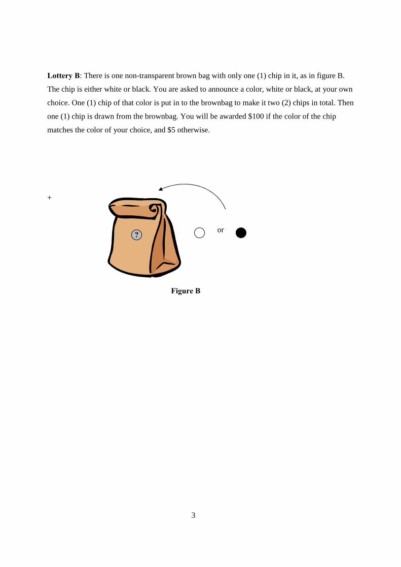
Lottery B: There is one non-transparent brown bag with only one (1) chip in it, as in figure B.

The chip is either white or black. You are asked to announce a color, white or black, at your own

choice. One (1) chip of that color is put in to the brownbag to make it two (2) chips in total. Then

one (1) chip is drawn from the brownbag. You will be awarded $100 if the color of the chip

matches the color of your choice, and $5 otherwise.

+

Figure B

or ?

4

Lottery C: There are two (2) non-transparent brown bags each with four (4) chips in it, as in

figure C. The first bag contains one (1) white chip and three (3) black chips. The second bag

contains four (4) white chips. You are asked to announce a color, white or black, at your own

choice. After your announcement, we will roll a fair die in front of you. If it ends up with 1 or 2

on the top, we will use the first bag; otherwise, we use the second bag. Then one (1) chip is

drawn from the chosen bag. You will be awarded $100 if the color of the chip matches the color

of your choice, and $5 otherwise.

Figure C

5

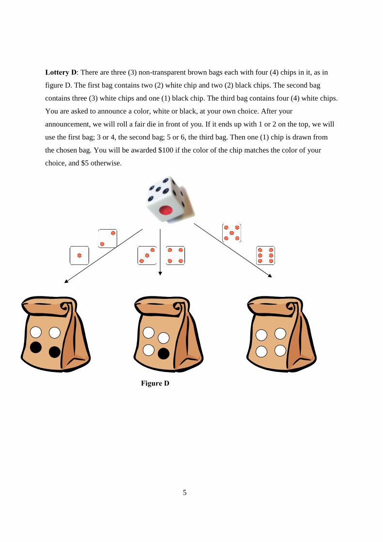
Lottery D: There are three (3) non-transparent brown bags each with four (4) chips in it, as in

figure D. The first bag contains two (2) white chip and two (2) black chips. The second bag

contains three (3) white chips and one (1) black chip. The third bag contains four (4) white chips.

You are asked to announce a color, white or black, at your own choice. After your

announcement, we will roll a fair die in front of you. If it ends up with 1 or 2 on the top, we will

use the first bag; 3 or 4, the second bag; 5 or 6, the third bag. Then one (1) chip is drawn from

the chosen bag. You will be awarded $100 if the color of the chip matches the color of your

choice, and $5 otherwise.

Figure D

6

Lottery preferences:

If you are sure about how these lotteries operate, please take a moment to evaluate them and

then rank them according to your preference. Suppose you are given a chance to enter for one of

the lotteries, which one would you like most? If that one is not available, which will come in as

second choice and so forth?

Please note that your answer will help decide which lottery you will get if you are chosen to

take part in a real one, and hence it may affect your potential payoff. So, please take your time,

try to understand how each lottery works before you put down your preference.

If you have made your choices, please print the letters associated with each lottery (A, B, C

or D) in one of the boxes in your questionnaire: most preferred (rank 1); somewhat preferred

(rank 2); less preferred (rank 3) or least preferred (rank 4).

Please put only one letter in each box. If you feel you cannot decide between two or more

lotteries, you may put them in adjacent boxes and put an equal sign “=” in between. However, if

you are to be chosen to play in our realized lottery and the two lotteries available deemed

“equal” by you, we will pick one for you to participate.

Most Preferred

(Rank 1)

Somewhat Preferred

(Rank 2)

Less Preferred

(Rank 3)

Least Preferred

(Rank 4)

Thanks for your participation. Please do not forget to sign the next page.