How Much Ambiguity Aversion?Finding Indifferences between Ellsberg’s

Risky and Ambiguous Bets

Ken BinmoreEconomics DepartmentUniversity College LondonLondon WC1E 6BT, UK

Lisa StewartPsychology DepartmentAustralian National UniversityCanberra ACT 0200, Australia

Alex Voorhoeve (corresponding author)Department of Philosophy, Logic and Scientific MethodLondon School of EconomicsLondon WC2E 2AE, UK

tel: +44-20-7955-6579fax: +44-20-7955-6845email: a.e.voorhoeve@lse.ac.uk

Abstract: Experimental results on the Ellsberg paradox typically revealbehavior that is commonly interpreted as ambiguity aversion. The exper-iments reported in the current paper find the objective probabilities fordrawing a red ball that make subjects indifferent between various risky anduncertain Ellsberg bets. They allow us to examine the predictive power ofalternative principles of choice under uncertainty, including the objectivemaximin and Hurwicz criteria, the sure-thing principle, and the principle ofinsufficient reason. Contrary to our expectations, the principle of insufficientreason performed substantially better than rival theories in our experiment,with ambiguity aversion appearing only as a secondary phenomenon.

Keywords: ambiguity aversion, Ellsberg paradox, Hurwicz criterion, max-imin criterion, principle of insufficient reason.

JEL classification: C91, D03.

How Much Ambiguity Aversion?Finding Indifferences between Ellsberg’s

Risky and Ambiguous Bets

Ken Binmore, Lisa Stewart, and Alex Voorhoeve1

1 Ellsberg Paradox

Daniel Ellsberg [12] famously proposed an experiment the results of which havebecome known as the “Ellsberg paradox” because they are inconsistent with thepredictions of expected utility theory.

Figure 1: Ellsberg paradox: In the version illustrated an urn contains ten red ballsand another twenty balls of which it is only known that they are either black orwhite. A ball is chosen at random from the urn, the color of which determinesthe award of a prize (which is here taken to be one dollar). Whether subjects winor lose depends on which of the lottery tickets J , K, L, or M they are holding.

In one version of Ellsberg’s experiment, a ball is drawn from an urn containingten red balls and twenty other balls, of which it is known only that each is eitherblack or white. The gambles J , K, L, and M in Figure 1 represent various rewardschedules depending on the color of the ball that is drawn. Ellsberg predicted that

1Parts of the experimental data were gathered while Lisa Stewart was a researcher in theHarvard Psychology Department and Alex Voorhoeve was a Faculty Fellow at Harvard’s SafraCenter for Ethics. We thank the Decision Science Laboratory at Harvard’s Kennedy School ofGovernment and the ELSE laboratory at University College London for the generous use of theirfacilities, and the Suntory and Toyota International Centres for Economics and Related Disciplines(STICERD) for financial support. Ken Binmore thanks the British Economic and Social ResearchCouncil through the Centre for Economic Learning and Social Evolution (ELSE), the British Artsand Humanities Research Council through grant AH/F017502 and the European Research Councilunder the European Community’s Seventh Framework Programme (FP7/2007-2013)/ERC grant295449. Alex Voorhoeve thanks the Safra Center for Ethics for its Faculty Fellowship and theBritish Arts and Humanities Research Council through grant AH/J006033/1. Results were pre-sented at Bristol University, the European University Institute in Florence, Harvard University, theLSE, the University of Siena, and the University of York (UK). We thank Richard Bradley, BarbaraFasolo, Joshua Greene, Glenn Harrison, Jimmy Martinez, Katie Steele, Joe Swierzbinski, PeterWakker, and those present at our seminars for their comments.

1

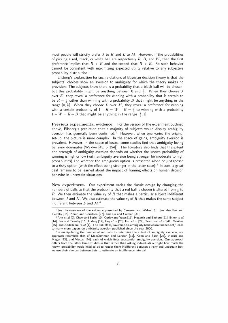
most people will strictly prefer J to K and L to M . However, if the probabilitiesof picking a red, black, or white ball are respectively R, B, and W , then the firstpreference implies that R > B and the second that B > R. So such behaviorcannot be consistent with maximizing expected utility relative to any subjectiveprobability distribution.

Ellsberg’s explanation for such violations of Bayesian decision theory is that thesubjects’ choices show an aversion to ambiguity for which the theory makes noprovision. The subjects know there is a probability that a black ball will be chosen,but this probability might be anything between 0 and 2

3. When they choose J

over K, they reveal a preference for winning with a probability that is certain tobe R = 1

3rather than winning with a probability B that might be anything in the

range [0, 23]. When they choose L over M , they reveal a preference for winning

with a certain probability of 1 − R = W + B = 23

to winning with a probability1 − W = R + B that might be anything in the range [ 1

3, 1].

Previous experimental evidence. For the version of the experiment outlinedabove, Ellsberg’s prediction that a majority of subjects would display ambiguityaversion has generally been confirmed.2 However, when one varies the originalset-up, the picture is more complex. In the space of gains, ambiguity aversion isprevalent. However, in the space of losses, some studies find that ambiguity-lovingbehavior dominates (Wakker [45, p. 354]). The literature also finds that the extentand strength of ambiguity aversion depends on whether the known probability ofwinning is high or low (with ambiguity aversion being stronger for moderate to highprobabilities) and whether the ambiguous option is presented alone or juxtaposedto a risky option (with the effect being stronger in the latter case).3 In sum, a greatdeal remains to be learned about the impact of framing effects on human decisionbehavior in uncertain situations.

New experiment. Our experiment varies the classic design by changing thenumbers of balls so that the probability that a red ball is chosen is altered from 1

3to

R. We then estimate the value r1 of R that makes a particular subject indifferentbetween J and K. We also estimate the value r2 of R that makes the same subjectindifferent between L and M .4

2See the overview of the evidence presented by Camerer and Weber [8]. See also Fox andTversky [15], Keren and Gerritsen [27], and Liu and Colman [31].

3Ahn et al [2], Chow and Sarin [10], Curley and Yates [11], Hogarth and Einhorn [21], Etner et al[14], Fox and Tversky [15], Halevy [19], Hey et al [20], Hsu et al [22], Trautman et al [42], Wakker[45], and Abdellaoui et al [1]. The link http://aversion-to-ambiguity.behaviouralfinance.net/ leadsto many more papers on ambiguity aversion published since the year 2000.

4In manipulating the number of red balls to determine the extent of ambiguity aversion, ourapproach resembles that of MacCrimmon and Larsson [32], Kahn and Sarin [25], Viscusi andMagat [43], and Viscusi [44], each of which finds substantial ambiguity aversion. Our approachdiffers from the latter three studies in that rather than asking individuals outright how much theknown probability would need to be to render them indifferent between a risky and uncertain bet,we use their choices between bets to estimate an indifference interval.

2

A subject who honors Savage’s [38, p. 21] sure-thing principle will have

r1 = r2. (1)

The rationale in our special case is that, in comparing J and K and in comparingL and M , what happens if a white ball is drawn is irrelevant. The two comparisonstherefore depend only on what happens if a white ball is not drawn. But if a red orblack ball is sure to be drawn, then J is the same as M and K is the same as L.So J and K should be regarded as being worth the same if and only if the same istrue of L and M .

Given the widespread finding of ambiguity aversion in the classic Ellsberg para-dox, our aim in this paper was to examine the extent to which the Hurwicz criteriondiscussed in the next section explains deviations from the sure-thing principle andother tenets of Bayesian decision theory caused by ambiguity aversion.

2 Theories

We consider various theories of choice behavior under uncertainty. Figure 2 illus-trates the behavior predicted by each of the principles reviewed. These all havevariants that apply when the outcomes are not merely winning or losing as in ourpaper. For example, the Hurwicz criterion has been generalized to what is some-times called alpha-max-min (Ghirardato and Marinacci [16]). Our case is simplerbecause it leaves no room to maneuver about the nature of the utility function thatcan be attributed to a subject. We need only consider the (Von Neumann andMorgenstern) utility function that assigns a value of 0 to losing and 1 to winning.Difficulties about the level of a subject’s risk aversion and the like therefore do notarise in our experiment.

Maximin criterion (MXN). The most widely discussed alternative to Bayesiandecision theory was proposed by Wald [46] and has been developed since that timeby numerous authors (see Gilboa [17]). It sometimes goes by the name of themaximin criterion, because it predicts that subjects will proceed as though they arefacing the least favorable of all the probability distributions that ambiguity allows.

We consider Von Neumann’s version of the maximin criterion here.5 In thisobjective version, the decision-maker’s ambiguity is assumed to extend to all prob-ability distributions that are consistent with the objective data.

5The objective maximin criterion is often referred to as the minimax criterion. The confusionbetween maximin and minimax presumably arises because minimax equals maximin in Von Neu-mann’s famous minimax theorem. The confusion is sometimes compounded because Savage [38]proposed a further decision criterion called the minimax regret criterion, which happens to makethe same predictions as the maximin criterion in the special case considered in this paper. (Savage[38, p. 16] distinguished between large and small worlds, recommending his minimax regret crite-rion for the former. He variously describes using Bayesian decision theory outside a small world as“preposterous” and “utterly ridiculous”.)

3

Applying the objective maximin criterion to our example, we are led to seek tomaximize a utility function defined by u(J) = R, u(K) = 0, u(L) = 1 − R, andu(M) = R. So for 0 < R < 1

2, J is preferred to K and L to M .

The literature also features a subjective version of the maximin criterion in whichthe decision-maker may have internal reasons for excluding some of the probabilitydistributions taken into account by the objective version (Gilboa and Schmeidler[18]). Applying the subjective maximin criterion in the extreme case when thedecision-maker considers only a single probability distribution gives the same pre-dictions as the sure-thing principle. If we insist on some ambiguity, the class ofsubjective versions of the maximin criterion coincides with the notion of weak am-biguity aversion to be considered later.

Hurwicz criterion (HWZ). The Hurwicz criterion [23] goes back to the be-ginnings of decision theory. Hurwicz’s proof was simplified by Arrow [3]. As aconsequence, it is sometimes referred to as the Arrow-Hurwicz criterion. It featuresin Luce and Raiffa’s [30] discussion of decisions made under complete ignorance intheir book Games and Decisions. Ellsberg [13] considers it at length in his Risk,Ambiguity, and Decision, both as a normative criterion and as an explanation forambiguity-averse choices. Binmore [4, p. 166] offers a normative defense of a mul-tiplicative version of the Hurwicz criterion, which would be indistinguishable fromthe standard (additive) Hurwicz criterion in our experiment. For a review of thecriterion’s role in the literature, see Etner et al [14].

At an early stage, Milnor [33] offered axioms that characterize several of thedecision criteria considered in this paper. In the case of the Hurwicz criterion,he replaces a version of the standard independence axiom, which he calls columnlinearity, by a new axiom that he calls column duplication. This axiom says thatthe decision maker’s choice will remain unchanged if a new state is appended fromwhich the same consequences as an existing state would follow for every choiceavailable to the decision maker. The idea is that a completely ignorant decisionmaker will have no reason not to assimilate the new state into the existing statethat it duplicates.

We follow Milnor in regarding the Hurwicz criterion as applicable in situationsof partial ignorance only after the decision maker’s partial knowledge has beenincorporated into her model in terms of objective upper and lower probabilities thatbound the possible range of the probability R that a red ball is drawn. Subjectiveversions of the Hurwicz criterion are possible, but we only consider the objectiveversion.

The standard Hurwicz criterion balances the pessimism of the objective max-imin criterion against the optimism of what might be called the objective maximaxcriterion. The Hurwicz criterion values a gamble G offering a prize with probabilityP with the utility function

u(G) = (1 − h)P + hP , (2)

4

where [P , P ] is the (objective) range of possible values of P , and the constant h(0 ≤ h ≤ 1) registers how averse the subject is to ambiguity. The case h = 0 ofmaximal aversion coincides with the objective maximin criterion. The case h = 1corresponds to the objective maximax criterion. The case h = 1

2is indistinguishable

from the principle of insufficient reason in our experiment.In our example, the Hurwicz criterion yields u(J) = R, u(K) = h(1 − R),

u(L) = 1 − R, and u(M) = (1 − h)R + h. If a subject is indifferent between Jand K when R = r1, it follows that h = r1/(1 − r1). Similarly, if the subject isindifferent between L and M when R = r2, then h = (1−2r2)/(1−r2). Assumingthat the same value of h applies in both cases, it follows that the Hurwicz criterionpredicts that r1 and r2 are connected by the equation6

(3r1 − 2)(3r2 − 2) = 1 . (3)

Sure-thing principle (STP). The Hurwicz criterion needs to be comparedwith the orthodox Bayesian approach (expected utility theory), which denies thatsubjects might be unable to resolve ambiguities about what subjective probabilityto assign to events. In this case, u(J) = R, u(K) = B, u(L) = W + B, andu(M) = R + W . So the criteria for indifference between J and K and between Land M are the same: r1 = R = B = r2.

We have already seen that we need no more than the sure-thing principle tojustify the conclusion that r1 = r2, which one might also categorize as representingambiguity neutrality.

Laplace’s principle of insufficient reason (PIR). This principle says thatevents should be assigned the same subjective probability if no reason can be givenfor regarding one event as more likely than another. A subject who believes this tobe true of drawing a black or a white ball will therefore assign them equal probability,so that W = B. When this result is combined with the equation r1 = R = B = r2,we obtain that

r1 = r2 = 13. (4)

This outcome is also predicted by the Hurwicz criterion with h = 12.

Weak ambiguity aversion (WAA). We say that r1 < r2 indicates weakambiguity aversion, because it implies that J � K and L � M when the probabilityR of a red ball being drawn lies between r1 and r2. Reversing the inequalitygenerates a criterion for weak ambiguity-loving behavior.

6Binmore’s [4, p. 166] multiplicative version of the Hurwicz criterion also yields equation (3) toa first order of approximation. To a second order of approximation, it yields

(3r1 − 2)(3r2 − 2) = 1 + c(r1 − r2){2(1 − r1)(1 − r2) − 1} ,

for some small positive constant c.

5

Outcomes that satisfy the Hurwicz criterion with h < 12

are ambiguity averse inboth the weak sense and the strong sense that follows.

Strong ambiguity aversion (SAA). We treat pairs (r1, r2) with r1 < 13

andr2 > 1

3as cases of strong ambiguity aversion. To see why, recall that a Bayesian

subject will express indifference between J and K when R = B. So if W = B, thenr1 = 1

3. If one regards behaving as though B < W as a manifestation of strong

ambiguity aversion, then r1 < 13. The requirement that r2 > 1

3is derived similarly.

Reversing all inequalities generates a criterion for strong ambiguity-loving behavior.

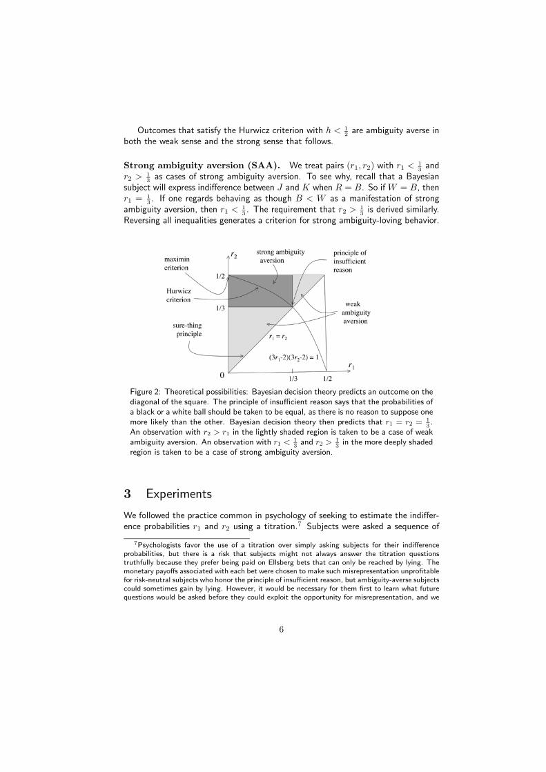
Figure 2: Theoretical possibilities: Bayesian decision theory predicts an outcome on thediagonal of the square. The principle of insufficient reason says that the probabilities ofa black or a white ball should be taken to be equal, as there is no reason to suppose onemore likely than the other. Bayesian decision theory then predicts that r1 = r2 = 1

3.

An observation with r2 > r1 in the lightly shaded region is taken to be a case of weakambiguity aversion. An observation with r1 < 1

3and r2 > 1

3in the more deeply shaded

region is taken to be a case of strong ambiguity aversion.

3 Experiments

We followed the practice common in psychology of seeking to estimate the indiffer-ence probabilities r1 and r2 using a titration.7 Subjects were asked a sequence of

7Psychologists favor the use of a titration over simply asking subjects for their indifferenceprobabilities, but there is a risk that subjects might not always answer the titration questionstruthfully because they prefer being paid on Ellsberg bets that can only be reached by lying. Themonetary payoffs associated with each bet were chosen to make such misrepresentation unprofitablefor risk-neutral subjects who honor the principle of insufficient reason, but ambiguity-averse subjectscould sometimes gain by lying. However, it would be necessary for them first to learn what futurequestions would be asked before they could exploit the opportunity for misrepresentation, and we

6

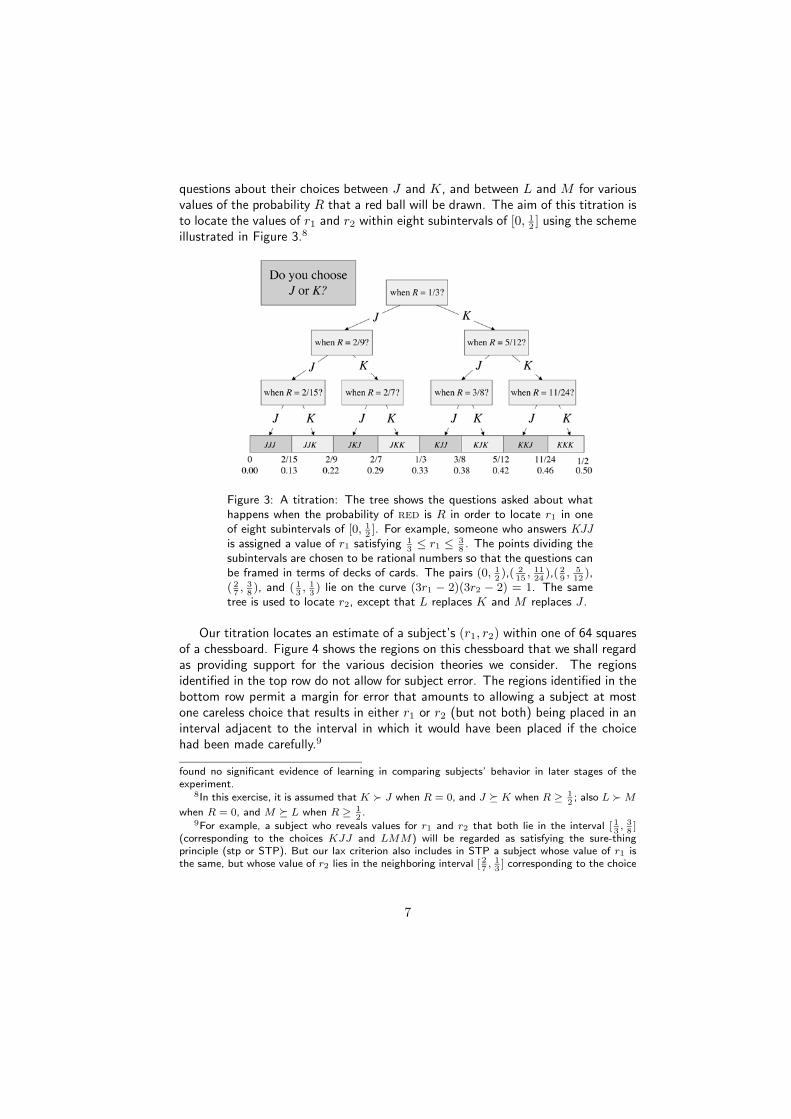
questions about their choices between J and K, and between L and M for variousvalues of the probability R that a red ball will be drawn. The aim of this titration isto locate the values of r1 and r2 within eight subintervals of [0, 1

2] using the scheme

illustrated in Figure 3.8

Figure 3: A titration: The tree shows the questions asked about whathappens when the probability of red is R in order to locate r1 in oneof eight subintervals of [0, 1

2]. For example, someone who answers KJJ

is assigned a value of r1 satisfying 13≤ r1 ≤ 3

8. The points dividing the

subintervals are chosen to be rational numbers so that the questions canbe framed in terms of decks of cards. The pairs (0, 1

2),( 2

15, 11

24),( 2

9, 5

12),

( 27, 3

8), and ( 1

3, 1

3) lie on the curve (3r1 − 2)(3r2 − 2) = 1. The same

tree is used to locate r2, except that L replaces K and M replaces J .

Our titration locates an estimate of a subject’s (r1, r2) within one of 64 squaresof a chessboard. Figure 4 shows the regions on this chessboard that we shall regardas providing support for the various decision theories we consider. The regionsidentified in the top row do not allow for subject error. The regions identified in thebottom row permit a margin for error that amounts to allowing a subject at mostone careless choice that results in either r1 or r2 (but not both) being placed in aninterval adjacent to the interval in which it would have been placed if the choicehad been made carefully.9

found no significant evidence of learning in comparing subjects’ behavior in later stages of theexperiment.

8In this exercise, it is assumed that K � J when R = 0, and J � K when R ≥ 12; also L � M

when R = 0, and M � L when R ≥ 12.

9For example, a subject who reveals values for r1 and r2 that both lie in the interval [ 13, 38]

(corresponding to the choices KJJ and LMM) will be regarded as satisfying the sure-thingprinciple (stp or STP). But our lax criterion also includes in STP a subject whose value of r1 isthe same, but whose value of r2 lies in the neighboring interval [ 2

7, 13] corresponding to the choice

7

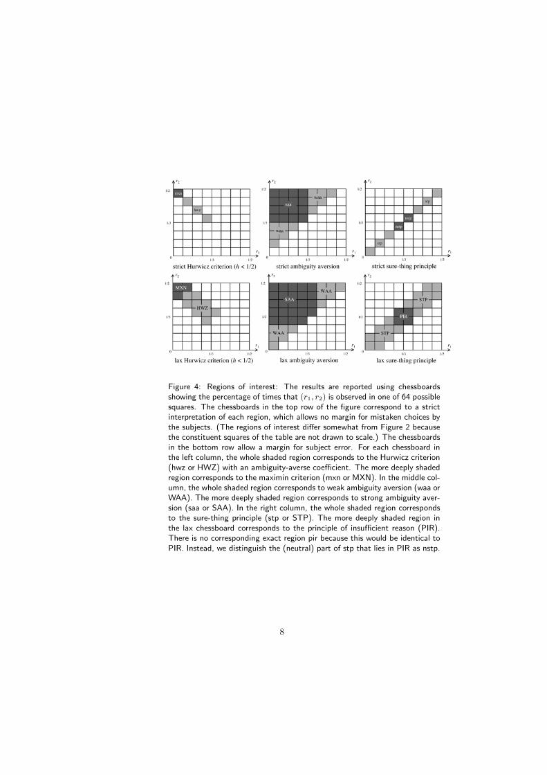
Figure 4: Regions of interest: The results are reported using chessboardsshowing the percentage of times that (r1, r2) is observed in one of 64 possiblesquares. The chessboards in the top row of the figure correspond to a strictinterpretation of each region, which allows no margin for mistaken choices bythe subjects. (The regions of interest differ somewhat from Figure 2 becausethe constituent squares of the table are not drawn to scale.) The chessboardsin the bottom row allow a margin for subject error. For each chessboard inthe left column, the whole shaded region corresponds to the Hurwicz criterion(hwz or HWZ) with an ambiguity-averse coefficient. The more deeply shadedregion corresponds to the maximin criterion (mxn or MXN). In the middle col-umn, the whole shaded region corresponds to weak ambiguity aversion (waa orWAA). The more deeply shaded region corresponds to strong ambiguity aver-sion (saa or SAA). In the right column, the whole shaded region correspondsto the sure-thing principle (stp or STP). The more deeply shaded region inthe lax chessboard corresponds to the principle of insufficient reason (PIR).There is no corresponding exact region pir because this would be identical toPIR. Instead, we distinguish the (neutral) part of stp that lies in PIR as nstp.

8

The principle of insufficient reason (PIR) requires special treatment because 13

isan endpoint of two of our intervals. Any value of (r1, r2) that lies in one of the foursquares of our chessboard with a corner at ( 1

3, 1

3) is therefore treated as supporting

PIR. This region is not expanded to include subjects’ choices in intervals adjacentto these four squares because subjects who intended to act in conformity with PIRwould be indifferent between J and K (and between L and M) for r1 = 1

3. It

follows that if their choices were to place them in a square adjacent to the foursquares that have [ 1

3, 1

3] as a midpoint, then they would have strayed further from

their true preference than subjects who intended to act in accordance with one ofthe other principles and who ended up in a square adjacent to a region permitted bythat principle. For similar reasons, we do not shrink PIR to obtain a smaller regionpir. The region nstp in Figure 4 should be thought of only as the neutral part ofstp.

It will be necessary to consider the extent to which apparent support for onetheory needs to be assessed in the light of the support which the same data givesan alternative theory. For example, a fraction of the data that is consistent withweak ambiguity aversion (WAA) also supports the principle of insufficient reason(PIR). In considering such issues, we use the notation WAA\PIR, which consists ofall squares on the chessboard in the region WAA but not in the region PIR.

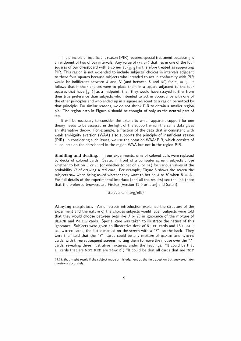
Shuffling and dealing. In our experiments, urns of colored balls were replacedby decks of colored cards. Seated in front of a computer screen, subjects chosewhether to bet on J or K (or whether to bet on L or M) for various values of theprobability R of drawing a red card. For example, Figure 5 shows the screen thesubjects saw when being asked whether they want to bet on J or K when R = 5

12.

For full details of the experimental interface (and all the results) see the link (notethat the preferred browsers are Firefox [Version 12.0 or later] and Safari):

http://alkami.org/ells/

Allaying suspicion. An on-screen introduction explained the structure of theexperiment and the nature of the choices subjects would face. Subjects were toldthat they would choose between bets like J or K in ignorance of the mixture ofblack and white cards. Special care was taken to illustrate the nature of thisignorance. Subjects were given an illustrative deck of 6 red cards and 15 black

or white cards, the latter marked on the screen with a “?” on the back. Theywere then told that the “?” cards could be any mixture of black and white

cards, with three subsequent screens inviting them to move the mouse over the “?”cards, revealing three illustrative mixtures, under the headings: “It could be thatall cards that are not red are black”; “It could be that all cards that are not

MLL that might result if the subject made a misjudgment at the first question but answered laterquestions accurately.

9

Figure 5: Experimental interface: When confronted with thisparticular interface, the subject is being asked whether he or sheprefers J or K when the probability of drawing a red card isR = 5

12.

red are white”; and “It could be that all cards that are not red are any of themany possible mixtures of black and white, for example . . . ”, with the exampleconsisting of 5 white and 10 black cards.

Inspired by Hey et al [20], we sought to allay any suspicion of deceit on our partby making transparent the preparation of the decks from which a winning card wouldbe drawn. After making two practice choices, subjects were invited to the front ofthe room to witness one of the practice bets being played for illustrative purposesonly. The experimenter opened a box of red cards and box of black or white

cards, and counted out the number of red and black or white cards in thefirst practice choice (respectively 6 and 15). These were placed in a card-shufflingmachine to randomize the order of the deck. Finally, a subject exposed the third cardfrom the top in the shuffled deck, the color of which determined whether subjectshad won or lost. Subjects were told, truthfully, that of the subsequent 24 choicesthey faced in the real experiment, two bets would be randomly selected by thecomputer to be played for money in this manner at the end of the experiment, withthe choices they had made determining the winning color(s). (This randomizationwas done for each subject individually, so that all subjects had tailor-made betsconstructed and played for them.)

This procedure may be relevant to the relatively low levels of ambiguity aversionwe observed. For example, Pulford [35] reports significantly more ambiguity aversionafter drawing attention to the possibility of experimental deceit. If a subject believesthat the experimenter is deceitfully manipulating the shuffling-and-dealing protocolsto minimize payoffs (or for some other reason), then the problem faced by the subjectceases to be a one-person decision problem and becomes instead a game playedbetween the subject and the experimenter (Brewer [7], Schneeweiss [40], Kadane[24]). In an extreme case, the subject may (unconsciously?) perceive this game aszero-sum, in which rational play (according to Bayesian decision theory) requires

10

the play of the subject’s maximin strategy (Schneeweiss [40]). Researchers are thenat risk of misinterpreting such play as the use of an ambiguity-averse strategy in aone-person decision problem.10

Subjects. Two types of subject were studied: on-site subjects and on-line sub-jects. The on-site participants were recruited from lists of volunteers maintainedby the laboratories at which various versions of the experiment were run. Thesesubjects were paid according to their success in selecting winning cards. On-linesubjects participated from remote sites with negligible payment (and without theopportunity to check up on how the cards were shuffled and dealt).11 The behaviorof on-line subjects turned out to resemble that of on-site subjects, but is muchnoisier. (The hypothesis that on-line subjects paid less attention to their choiceproblem than on-site subjects is supported by the fact that the mean response timeof on-line subjects to each choice was just over half the mean response time ofon-site subjects.) The discussion that follows therefore focuses on the on-site data.

3.1 Version 1

Following the practice choices and demonstration session, the subjects returned totheir screens and were taken through the experiment with the aid of a computerizedinterface. The on-site edition of Version 1 of the experiment was run at the HarvardDecision Science Laboratory, using the Harvard Psychology Department subjectpool. A pilot that led to some minor design changes is not reported. The aim wasto elicit from each subject four pairs of observations for the indifference intervals inwhich to locate r1 and r2. The experiment had five stages:

1. At the beginning of Round 1, subjects were told that the round had the followingfour parts, with the choices in each part being constructed from the same decks.Subjects were not told that the probability R of a red card would vary according tothe titration of Figure 3.

(a) Three choices between J (red wins) and K (black wins).(b) Three choices between J and K ′ (white wins).(c) Three choices between L (white and black win) and M (red and white

win). (Note that L was described as “not-red wins”, and M as “not-black

wins”.)(d) Three choices between L and M ′ (red and black win). (Note that L was

described as “not-red wins”, and M ′ as “not-white wins”.)

10Savage [38, p. 16] would perhaps have commented that leaving room for suspicion of dishonestmanipulation by the experimenter creates a large world for the subjects. Our design is intended tomake the subjects’ world small in this respect.

11We used Amazon’s Mechanical Turk (https://www.mturk.com), Psychological Research onthe Net (http://psych.hanover.edu/Research/exponnet.html), and the Research Subject VolunteerProgram (http://alkami.org ¡http://alkami.org/¿). Participants recruited via Mechanical Turkwere paid a token $0.05 for completing the approximately six-minute study.

11

Items (a) and (c) above determined one estimate of (r1, r2) to be compared withFigure 4. Items (b) and (d) determined a second estimate.

2. Round 2 was identical to Round 1, save that yellow replaced white and blue

replaced black. This round therefore provided a further two estimates of (r1, r2).3. Subjects were taken one-by-one through the questions from a Life OrientationTest as revised by Scheier et al [39].

4. Subjects were asked five questions about whether the tasks and questions hadbeen clear, and whether any problems arose during the experiment.

5. Two gambles (one from each round) were chosen at random by the computerfor each subject to be played for real. (The prizes were chosen to render subjectschoosing according to the principle of insufficient reason indifferent about whichof their choices were played for real.) On-site subjects left the laboratory with anaverage of $22.

The data from Version 1 are displayed in Figure 6 and summarized in Table 1. Adetailed analysis follows below. Here, we note two things which surprised us. First,though there was some evidence for ambiguity aversion, there was not as much asour reading of the literature had led us to expect. Second, we were disappointed notto find much support for the Hurwicz criterion for any value of h except those around12, for which the principle of insufficient reason offers a competing explanation.

3.2 Version 2

One possible explanation we considered was that the framing of the choices betweenL and M as between “not-black wins” and “not-red wins” affected thesubjects. (The analogous ’not’-description was given for the choices between L andM ′.) In order to establish whether this was a key factor, we ran Version 2, whichis exactly the same as Version 1 except for a change in how the problems facedby the subjects are framed, substituting the description “black and white” for“not-red”, “red and white” for “not-black”, and so on. The on-site versionof this new experiment was carried out in the ELSE laboratory at University CollegeLondon with 76 on-site subjects.12

Though, as our analysis in Section 5.2 shows, the results of the on-site subjectsfor Version 2 differed significantly in some respects from the results of the on-sitesubjects for Version 1, they were similar in that they displayed only limited evidenceof ambiguity aversion and provided little support for the Hurwicz criterion otherthan with h in the neighborhood of 1

2.

12The prizes were approximately equal to their previous dollar values but were denominated inBritish pounds. The average payout was around £13.

12

3.3 Version 3

We remained surprised not to see more ambiguity aversion in Version 2. A possibleexplanation proposed by Raiffa [36] is that on-site subjects could theoretically con-vert the problem into one in which an unambiguous distribution is available thatassigns black and white equal probabilities if they believed our (true) claims that:

1. They would face the same decision tree for the red versus black, red versuswhite, and all subsequent versions of the J versus K and J versus K ′ choices(and the iterations of the L versus M and L versus M ′ choices);

2. The decks involved in these choices would all be constructed from the same setof black or white (or blue or yellow) decks;

3. Each of the subjects’ choices was equally likely to be played for real.

No appeal to the principle of insufficient reason is then necessary to justifyplaying according to its tenets. To see why, consider the strategy of choosingblack when offered the choice between red and black, and choosing white

when offered the analogous choice between red and white. For a subject whoheld the aforementioned three beliefs, in Versions 1 and 2 of our experiment, thisstrategy is equivalent to turning down red in favor of an equiprobable lotterybetween black and white, with a probability 1

3of winning.

Consider next the strategy of choosing black when offered the choice betweenred and black, and choosing red and white when offered the choice betweenred and white and black and white. For a subject who held the afore-mentioned three beliefs, this is equivalent to turning down an equiprobable lotterybetween red and black and white in favor of an equiprobable lottery betweenblack and red and white. The latter has a probability 1

2of winning.

Of these two strategies, the first seems simpler, as it merely involves observingthat in every lottery in which one chooses black, one need only choose white

in an otherwise identical subsequent lottery in order to eliminate ambiguity. Thesecond strategy, by contrast, requires seeing that one needs to pair one’s choices inone kind of lottery (betting on a single color) with one’s choices in another kind oflottery (with two winning colors).

We do not regard it as plausible that a significant number of subjects employedeither of these strategies, because neither strategy seems particularly easy for sub-jects to grasp. Aside from other considerations, subjects who reason in this waywould need to apply some version of the Compound Lottery Axiom that Halevy [19]has found significant in distinguishing between those subjects classified as ambiguityaverse and those who are not.

Notwithstanding our doubts about the likelihood that subjects would form therequisite beliefs and employ one of these strategies, we decided to check whetherthe low level of ambiguity aversion might nonetheless be partly explained in this way.We therefore ran Version 3 of the experiment, again in the ELSE lab at UniversityCollege London. In this version, we eliminated the choices between J and K ′

and L and M ′, thereby removing the possibility of a subject using the simpler of

13

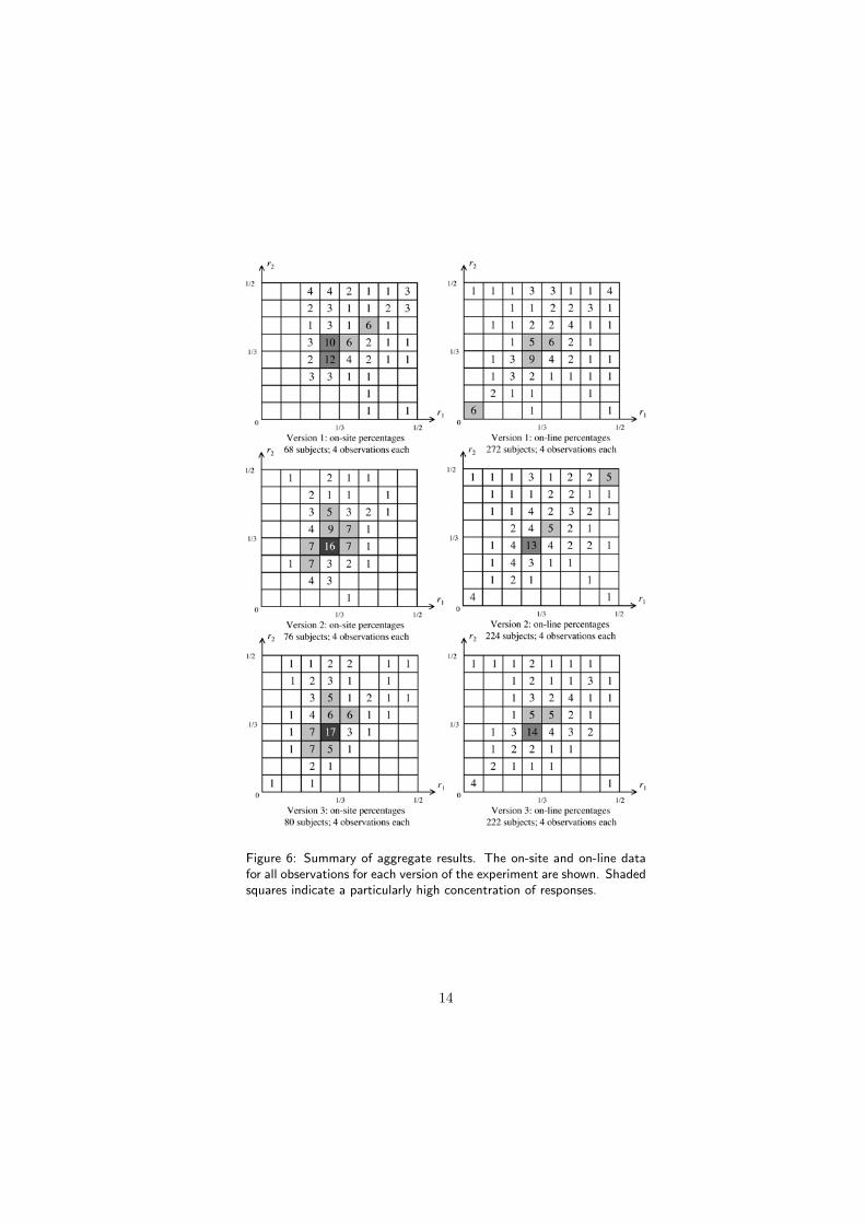
Figure 6: Summary of aggregate results. The on-site and on-line datafor all observations for each version of the experiment are shown. Shadedsquares indicate a particularly high concentration of responses.

14

the ambiguity-eliminating strategies mentioned above. Each round in the previousversions therefore became half as long. In order to keep the number of choicesfaced by each subject identical to the previous versions, we added two further shortrounds, which repeated the first round with different colors. To be precise:

1. As before, in Round 1, the subjects were first navigated through the tree ofFigure 3 to estimate the interval in which to locate the value r1 that makes asubject indifferent between J (red wins) and K (black wins). Subjects werethen navigated through a similar tree to estimate the value r2 that makes a subjectindifferent between L and M .

2. Subsequent rounds repeated this round with black replaced by blue, yellow,and green, respectively.

4 Aggregate Results

We had thought that the subjects might learn or otherwise adjust their behaviorover time, but the final round data is not significantly different from earlier roundsand so we aggregate the data across all rounds in each version of the experiment.The aggregated results of all three versions of the experiment both for on-site andon-line subjects are given as percentages of the total number of observations inFigure 6.

Table 1 summarizes our results. A crude criterion in assessing a theory is whetherit predicts better than the null hypothesis that subjects answer all questions atrandom. The first column of the table therefore shows the percentage of times anobservation would be made in the long run under this hypothesis. At first sight,all the theories considered seem to pass this test except for the objective maximincriterion (MXN). But how much does the sure-thing principle (STP) explain that isnot already explained by the principle of insufficient reason (PIR)? Since STP\PIRdoes no better than the null hypothesis in the on-site versions of the experiment,the answer would seem to be nothing at all in these versions.

The same reasoning also applies when one asks how much weak or strong ambi-guity aversion (WAA or SAA) or the Hurwicz criterion (HWZ with h < 1

2) explain

that is not explained by STP (now interpreted as a measure of approximate ambi-guity neutrality). All of HWZ\STP, WAA\STP, and SAA\STP perform no betterthan the null hypothesis. However, if all the data points in STP are excluded fromthe population (so that POP is replaced by POP\STP) as in the lower part of thetable for ‘lax criteria’, then each of HWZ\STP, WAA\STP, and SAA\STP performssignificantly better than the null hypothesis in on-site Versions 2 and 3 of the ex-periment. This provides some evidence for ambiguity aversion among subjects whoare not approximately ambiguity-neutral.

15

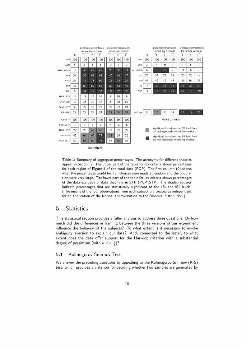
Table 1: Summary of aggregate percentages. The acronyms for different theoriesappear in Section 2. The upper part of the table for lax criteria shows percentagesfor each region of Figure 4 of the total data (POP). The first column (0) showswhat the percentages would be if all choices were made at random and the popula-tion were very large. The lower part of the table for lax criteria shows percentagesof the data exclusive of data that falls in STP (POP\STP). The shaded squaresindicate percentages that are statistically significant at the 1% and 5% levels.(The means of the four observations from each subject are treated as independentfor an application of the Normal approximation to the Binomial distribution.)

5 Statistics

This statistical section provides a fuller analysis to address three questions. By howmuch did the differences in framing between the three versions of our experimentinfluence the behavior of the subjects? To what extent is it necessary to invokeambiguity aversion to explain our data? And, connected to the latter, to whatextent does the data offer support for the Hurwicz criterion with a substantialdegree of pessimism (with h << 1

2)?

5.1 Kolmogorov-Smirnov Test

We answer the preceding questions by appealing to the Kolmogorov-Smirnov (K-S)test, which provides a criterion for deciding whether two samples are generated by

16

the same probability distribution. It is important that the K-S test is non-parametric,because its use shows that some of our data is not normally distributed, which rulesout various alternative approaches, including the Chi-Square test.

With one-dimensional data, the K-S statistic T is obtained by computing theempirical cumulative distribution functions of the two samples to be compared.The value of T is then the maximum of the absolute difference between these twocumulative distribution functions. Low values of T indicate that the evidence is notgood enough to reject the null hypothesis that the two samples are from the samedistribution. To say that the null hypothesis is rejected at the 10% significance levelis to say that there is one chance in ten that we are wrong to argue that the twosamples do not come from the same distribution.13

Lopes et al [29] review the problem of applying the K-S test with multi-dimensional data. The problem arises because the manner in which the data pointsare ordered then becomes significant. Their very severe recommendation requiresmaximizing over all possible orderings of the data points. Such a procedure seemsappropriate when the data is otherwise unstructured, but we exploit the underlyingstructure of our problem by applying the orthodox one-dimensional K-S test sepa-rately to the sums of the columns, the sums of the rows, and the sums of both typesof diagonal in each of the 8 × 8 data matrices of Figure 6. We thereby examinethe marginal distributions of r1, r2, r1 + r2, and r1 − r2. The final expression is ofparticular interest because it can serve as a measure of how far a point (r1, r2) liesfrom the main diagonal r1−r2 = 0, where all the data would lie if the subjects wereall ambiguity neutral. The K-S test is more reliable when applied to the diagonalsthan to the rows and columns because the former data is sorted into 15 bins, andthe latter into only 8 bins.

5.2 Comparing Distributions

Table 2 shows K-S statistics for our data.14 To save on space, we abuse notation byusing r1 and r2 in this section to refer to our binned data rather than the continuousvariables our experiment is intended to estimate.

The data in Table 2 supports the following conclusions.

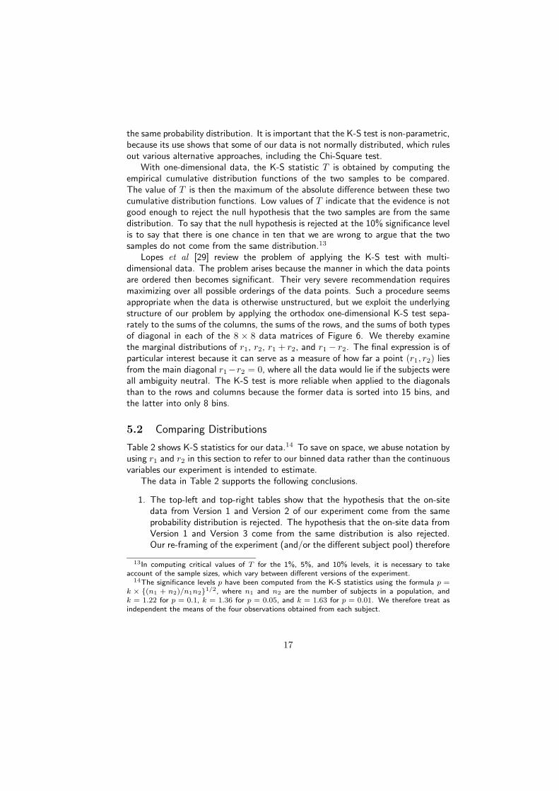
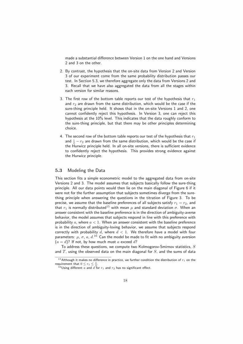
1. The top-left and top-right tables show that the hypothesis that the on-sitedata from Version 1 and Version 2 of our experiment come from the sameprobability distribution is rejected. The hypothesis that the on-site data fromVersion 1 and Version 3 come from the same distribution is also rejected.Our re-framing of the experiment (and/or the different subject pool) therefore

13In computing critical values of T for the 1%, 5%, and 10% levels, it is necessary to takeaccount of the sample sizes, which vary between different versions of the experiment.

14The significance levels p have been computed from the K-S statistics using the formula p =k × {(n1 + n2)/n1n2}1/2, where n1 and n2 are the number of subjects in a population, andk = 1.22 for p = 0.1, k = 1.36 for p = 0.05, and k = 1.63 for p = 0.01. We therefore treat asindependent the means of the four observations obtained from each subject.

17

made a substantial difference between Version 1 on the one hand and Versions2 and 3 on the other.

2. By contrast, the hypothesis that the on-site data from Version 2 and Version3 of our experiment come from the same probability distribution passes ourtest. In Section 5.3, we therefore aggregate only the data from Versions 2 and3. Recall that we have also aggregated the data from all the stages withineach version for similar reasons.

3. The first row of the bottom table reports our test of the hypothesis that r1

and r2 are drawn from the same distribution, which would be the case if thesure-thing principle held. It shows that in the on-site Versions 1 and 2, onecannot confidently reject this hypothesis. In Version 3, one can reject thishypothesis at the 10% level. This indicates that the data roughly conform tothe sure-thing principle, but that there may be other principles determiningchoice.

4. The second row of the bottom table reports our test of the hypothesis that r1

and 12− r2 are drawn from the same distribution, which would be the case if

the Hurwicz principle held. In all on-site versions, there is sufficient evidenceto confidently reject the hypothesis. This provides strong evidence againstthe Hurwicz principle.

5.3 Modeling the Data

This section fits a simple econometric model to the aggregated data from on-siteVersions 2 and 3. The model assumes that subjects basically follow the sure-thingprinciple. All our data points would then lie on the main diagonal of Figure 6 if itwere not for the further assumption that subjects sometimes diverge from the sure-thing principle when answering the questions in the titration of Figure 3. To beprecise, we assume that the baseline preferences of all subjects satisfy r1 = r2, andthat r1 is normally distributed15 with mean μ and standard deviation σ. When ananswer consistent with the baseline preference is in the direction of ambiguity-aversebehavior, the model assumes that subjects respond in line with this preference withprobability a, where a < 1. When an answer consistent with the baseline preferenceis in the direction of ambiguity-loving behavior, we assume that subjects respondcorrectly with probability d, where d < 1. We therefore have a model with fourparameters: μ, σ, a, d.16 Can the model be made to fit with no ambiguity aversion(a = d)? If not, by how much must a exceed d?

To address these questions, we compute two Kolmogorov-Smirnov statistics, Sand T , using the observed data on the main diagonal for S, and the sums of data

15Although it makes no difference in practice, we further condition the distribution of r1 on therequirement that 0 ≤ r1 ≤ 1

2.

16Using different a and d for r1 and r2 has no significant effect.

18

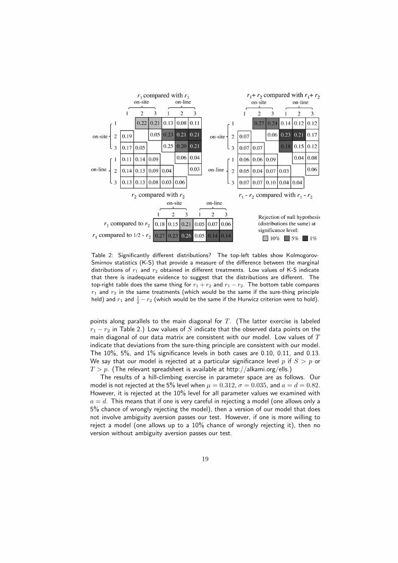
Table 2: Significantly different distributions? The top-left tables show Kolmogorov-Smirnov statistics (K-S) that provide a measure of the difference between the marginaldistributions of r1 and r2 obtained in different treatments. Low values of K-S indicatethat there is inadequate evidence to suggest that the distributions are different. Thetop-right table does the same thing for r1 + r2 and r1 − r2. The bottom table comparesr1 and r2 in the same treatments (which would be the same if the sure-thing principleheld) and r1 and 1

2− r2 (which would be the same if the Hurwicz criterion were to hold).

points along parallels to the main diagonal for T . (The latter exercise is labeledr1 − r2 in Table 2.) Low values of S indicate that the observed data points on themain diagonal of our data matrix are consistent with our model. Low values of Tindicate that deviations from the sure-thing principle are consistent with our model.The 10%, 5%, and 1% significance levels in both cases are 0.10, 0.11, and 0.13.We say that our model is rejected at a particular significance level p if S > p orT > p. (The relevant spreadsheet is available at http://alkami.org/ells.)

The results of a hill-climbing exercise in parameter space are as follows. Ourmodel is not rejected at the 5% level when μ = 0.312, σ = 0.035, and a = d = 0.82.However, it is rejected at the 10% level for all parameter values we examined witha = d. This means that if one is very careful in rejecting a model (one allows only a5% chance of wrongly rejecting the model), then a version of our model that doesnot involve ambiguity aversion passes our test. However, if one is more willing toreject a model (one allows up to a 10% chance of wrongly rejecting it), then noversion without ambiguity aversion passes our test.

19

By contrast, our model cannot be rejected at the 10% level when μ = 0.312,σ = 0.035, a = 0.90, and d = 0.80 (S = 0.04, T = 0.05). The parameter rangewithin which the latter conclusion can be maintained is small. This means that onlya version of our model which posits a modest degree of ambiguity aversion passesthe more stringent version of our test.

Notice that the fitted value of μ = 0.312 is close to 13

and that σ = 0.035is small. Our assumption that the subjects’ basic preferences honor the sure-thingprinciple is therefore sustained because the data is strongly concentrated in andaround the area predicted by the principle of insufficient reason. The analysis showsthat we cannot reconcile the model’s assumption about the subjects’ basic pref-erences without assuming random deviations from these basic preferences. Thesedeviations need to be biased in the direction of risk-averse behavior, but the degreeof bias is small.

For comparison, we also considered the same model with the Hurwicz criterionreplacing the sure-thing principle (so that subjects’ baseline preferences are assumednormal along the Hurwicz curve of Figure 2). For μ = 0.350 and σ = 0.050, thehypothesis that the new model is consistent with the data cannot be rejected atthe 5% level when a = d = 0.82 (S = 0.04, and T = 0.11). This result is not verysurprising when one notes that the Hurwicz criterion with h = 1

2is indistinguishable

from the principle of insufficient reason.In summary, our model best fits the data when it describes our population as if:

(i) Each subject’s baseline preferences approximate the principle of insufficientreason;

(ii) Each subject has a modest tendency to randomly diverge from these baselinepreferences, with diversion in an ambiguity-averse direction being somewhat morelikely.

Indeed, this version of our model cannot confidently be rejected. Our model-ing exercise therefore supports a modest degree of ambiguity aversion, but refutesversions of the Hurwicz criterion with h significantly less than 1

2.

6 Discussion

1. The principle of insufficient reason has the most predictive power in our ex-periment. About one third of our observations lie in the shaded region corre-sponding to PIR in Figure 4.

2. Theories that postulate a large level of ambiguity aversion all perform badlycompared with PIR.17 The objective maximin criterion performs very badly

17Recent working papers by Ahn et al [2] and Charness et al [9] report similar results with adifferent experimental design.

20

indeed.18 However, as evidenced by the lower part of Table 1 and our model,the data do provide evidence for a modest degree of ambiguity aversion.

3. Why do we not observe as much ambiguity aversion as is often reported? Onepossible reason is that our experimental protocol reduces suspicion of deceiton the part of the experimenter. A second potential reason is that Versions 1and 2 of our experiment allow sophisticated subjects to treat all probabilitiesas objective. However, levels of ambiguity aversion remain slight in Version3, where it is harder to pull off the same trick. A third reason is that ourambiguity aversion criteria are more demanding than in some studies, a pointthat we take up in the next item.

4. Our criteria for ambiguity aversion require that a subject be consistently am-biguity averse in two different (but related) comparisons. By contrast, someexperiments that report high levels of ambiguity aversion require a preferencefor a risky over an ambiguous option in only one comparison.19 But it ispresumably uncontroversial that ambiguity aversion judgments need to be re-liable to be a useful predictive tool in real-life situations. Figure 7 illustratesthat our more demanding criteria make a difference. If one were to pay at-tention only to estimates of r1, then one would find what would seem to besubstantial evidence for strong ambiguity aversion, especially in the case ofVersion 3 (where 73% of observations are consistent with strong ambiguityaversion as opposed to the 60–70% commonly reported).

5. Figure 7 also shows that part of the reason that our criteria make a differenceis that there is more ambiguity aversion in our one-winning-color choices (forwhich the indifference probability is r1) than in our two-winning-color choices(for which the indifference probability is r2). Our tentative conjecture isthat to some subjects, the ambiguous option is easier to discern in the one-winning-color case than in the two-winning-color case. In the one-winning-color case, the ambiguity present in betting on black is marked, and the lackof ambiguity in betting on red is obvious. By contrast, in the two-winning-color case, the ambiguity present in betting on red and white may be lessmarked to some (because subjects know the probability of part of the winning

18The same goes for the minimax regret criterion, since this coincides with the maximin criterionin our experiment.

19For example, Keren and Gerritsen [27] ask subjects to choose between betting on a red balldrawn from an urn which has a known probability of 1

3of yielding a red ball and betting on a green

ball or on a blue ball drawn from a different, ambiguous urn, in which green and blue togethermake up slightly more than 2

3of the balls. They conclude that a large majority preference for

betting on red is evidence of ambiguity aversion. Liu and Colman [31] similarly use a one-choicesetup. They offer subjects a choice between betting on a red ball drawn from an urn with a knownprobability of 1

2of yielding a red ball and betting on a red ball drawn from an urn containing red

and green balls in an unknown proportion. The prize from the uncertain urn was somewhat largerthan the prize from the risky urn. They take a majority preference to bet on red from the riskyurn to be evidence of ambiguity aversion.

21

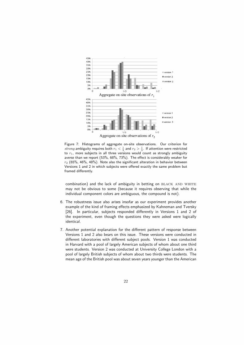
Figure 7: Histograms of aggregate on-site observations. Our criterion forstrong ambiguity requires both r1 < 1

3and r2 > 1

3. If attention were restricted

to r1, more subjects in all three versions would count as strongly ambiguityaverse than we report (53%, 68%, 73%). The effect is considerably weaker forr2 (65%, 46%, 48%). Note also the significant alteration in behavior betweenVersions 1 and 2 in which subjects were offered exactly the same problem butframed differently.

combination) and the lack of ambiguity in betting on black and white

may not be obvious to some (because it requires observing that while theindividual component colors are ambiguous, the compound is not).

6. The robustness issue also arises insofar as our experiment provides anotherexample of the kind of framing effects emphasized by Kahneman and Tversky[26]. In particular, subjects responded differently in Versions 1 and 2 ofthe experiment, even though the questions they were asked were logicallyidentical.

7. Another potential explanation for the different pattern of response betweenVersions 1 and 2 also bears on this issue. These versions were conducted indifferent laboratories with different subject pools. Version 1 was conductedin Harvard with a pool of largely American subjects of whom about one thirdwere students. Version 2 was conducted at University College London with apool of largely British subjects of whom about two thirds were students. Themean age of the British pool was about seven years younger than the American

22

pool.20 Though we therefore cannot be certain whether the difference is dueto framing effects or the composition of the subject pool, either way, this shiftcasts doubt on the robustness of subjects’ pattern of response in conditionsof uncertainty.

7 Psychological and Demographic Correlations

Psychologists define optimism and pessimism as positive and negative outcome ex-pectancies, and it has been proposed that people with a predisposition to expectingthings to turn out well might perceive an ambiguous situation differently from thoseexpecting things to turn out badly. Previous work has indicated an inverse relation-ship between ambiguity aversion and pessimism within the paradigm of the Ellsbergparadox (Pulford [35], Lauriola et al [28]). We therefore explored this relationshipmeasuring the degree of pessimism/optimism with the Life Orientation Test, Re-vised (LOT-R) of Scheier et al [39]. A subject’s ambiguity aversion was measuredby averaging r2 − r1 for the subject’s four choice sets, with a negative score indi-cating ambiguity-loving behavior, and a positive result indicating ambiguity-aversebehavior. These averaged scores ranged from -0.41 to 0.46 with a mean of 0.011(.081). LOT-R scores ranged from 0 (most pessimistic) to 24 (most optimistic),with a mean of 14.5 (5.0).21

We compared these measures of ambiguity aversion and pessimism/optimism foreach version separately for on-line and on-site participants using the Kruskal-Wallistest, Levenes’ test for equality of variances, independent samples t-tests, and scaledJZS Bayes Factors (Rouder et al [37]). Our measure of pessimism/optimism wasnot associated with ambiguity aversion.

Some research suggests that ambiguity aversion differs across genders (Borghanset al [6], Powell and Ansic [34]). However, no gender differences in mean ambiguityaversion were identified.

Comparisons of our measure of ambiguity aversion with other personal anddemographic variables also showed no robust correlation for any variable. A fullreport of these comparative analyses is available at http://alkami.org/ells.

8 Conclusion

Ambiguity aversion has been regularly observed in a majority of subjects’ choices inthe standard Ellsberg experiment. It is also regarded as a prevailing phenomenonfor choices involving gains generally. We designed a new experiment to examinehow much of this phenomenon could be explained by behavior in accordance withthe Hurwicz criterion. However, ambiguity aversion was less pronounced than inmany other studies and we found little evidence of behavior in accordance with

20Genders were roughly equal in each case.21These LOT-R results are consistent with the norms reported in Scheier et al [39].

23

the Hurwicz criterion. Indeed, the Hurwicz criterion with a substantial degree ofpessimism is clearly inconsistent with our findings. Only the principle of insufficientreason had marked predictive power in our experiment. We twice changed theframing of our experiment, which had a significant effect on some features of thesubjects’ behavior, but our basic conclusions were left unchanged.

We tentatively attribute our findings to two aspects of our study. First, weworked hard to eliminate suspicion that the experimenter might be manipulatingthe gambles. Second, our criteria for ambiguity aversion are more demanding thanin some studies because they require a subject to display aversion to the ambiguousoption in two different but related types of choices. Subjects whose choices do notmeet such strict criteria are not robustly ambiguity averse.

References

[1] M. Abdellaoui, A. Baillon, L. Placido, and P. Wakker. The Rich Domainof Uncertainty: Source Functions and Their Experimental Implementation.American Economic Review, 101:695–723, 2011.

[2] D. Ahn, S. Choi, D. Gale, and S. Kariv.Estimating Ambiguity Aversion in a Portfolio Choice Experiment.http://www.econ.nyu.edu/user/galed/papers.html, 2010.

[3] K. Arrow and L. Hurwicz. An Optimality Criterion for Decision Making underIgnorance. In Uncertainty and Expectations in Economics. Oxford, BasilBlackwell, 1972. (Edited by by C. Carter and J. Ford.)

[4] K. Binmore. Rational Decisions. Princeton University Press, Princeton, 2009.

[5] J. Bono and T. Judge. Core Self-Evaluations: A Review of the Trait and itsRole in Job Satisfaction. European Journal of Personality, 17:S5–S8, 2003.

[6] L. Borghans, J. Heckman, B. Golsteyn, and H. Meijers. Gender Differences inRisk and Ambiguity Aversion. Journal of the European Economic Associa-tion, 7:649–658, 2009.

[7] K. Brewer. Decisions under Uncertainty: Comment. Quarterly Journal ofEconomics, 79:657–653, 1965.

[8] C. Camerer and M. Weber. Recent Developments in Measuring Preferences:Uncertainty and Ambiguity. Journal of Risk and Uncertainty, 5:325–370,1992.

[9] G. Charness, E. Karni, and D. Levin. Ambiguity Attitudes: An ExperimentalInvestigation. http://ideas.repec.org/p/jhu/papers/590.html

[10] C. Chow and R. Sarin. Comparative Ignorance and Ambiguity Aversion. Jour-nal of Risk and Uncertainty, 22:129–139, 2001.

24

[11] S. Curley and J. Yates. An Empirical Evaluation of Descriptive Models of Am-biguity Reactions in Choice Situations. Journal of Mathematical Psychology,33:397–427, 1989.

[12] D. Ellsberg. Risk, Ambiguity and the Savage Axioms. Quarterly Journal ofEconomics, 75: 643–669, 1961.

[13] D. Ellsberg. Risk, Ambiguity, and Decision. Garland Publishing, New Yorkand London, 2001.

[14] J. Etner, M. Jeleva, and J.-M. Tallon. Decision Theory under Ambiguity.Journal of Economic Surveys, 26:324–270, 2012.

[15] C. Fox and A. Tversky. Ambiguity Aversion and Comparative Ignorance. Quar-terly Journal of Economics, 110:585–603, 1995.

[16] P. Ghirardato and M. Marinacci. Ambiguity Made Precise: A ComparativeFoundation. Journal of Economic Theory, 102:251–289, 2002.

[17] I. Gilboa. Uncertainty in Economic Theory: Essays in Honor of DavidSchmeidler’s 65th Birthday. Routledge, London, 2004.

[18] I. Gilboa and D. Schmeidler. Maximin Expected Utility with Non-Unique Prior.Journal of Mathematical Economics, 18:141–153, 1989.

[19] Y. Halevy. Ellsberg Revisited: An Experimental Study. Econometrica, 75:503–506, 2007.

[20] J. Hey, G. Lotito, and A. Maffioletti. The Descriptive and Predictive Ade-quacy of Decision Making under Uncertainty/Ambiguity. Journal of Risk andUncertainty, 41:81–111, 2010.

[21] R. Hogarth and H. Einhorn. Venture Theory: A Model of Decision Weights.Management Science, 36:780–803, 1990.

[22] M. Hsu, M. Bhatt, R. Adolphs, D. Tranel, and C. Camerer. Neural SystemsResponding to Degrees of Uncertainty in Human Decision Making. Science,310:1680–1683, 2005.

[23] L. Hurwicz. Optimality Criteria for Decision Making under Ignorance. CowlesCommission Discussion Paper, Statistics 370, 1951.

[24] J. Kadane. Healthy Scepticism as an Expected-Utility Explanation of the Phe-nomena of Allais and Ellsberg. In Decision-Making under Risk and Un-certainty: New Models and Empirical Findings. Kluwer, Dordrecht, 1992.(Edited by J. Geweke.)

[25] B. Kahn and R. Sarin. Modeling Ambiguity in Decisions under Uncertainty.Journal of Consumer Research, 15:265–272, 1988.

25

[26] D. Kahneman and A. Tversky. The Framing of Decisions and the Psychologyof Choice. Science, 211:453–458, 1981.

[27] G. Keren and L. Gerritsen. On the Robustness and Possible Accounts of Am-biguity Aversion. Acta Psychologica, 103:149–172, 1999.

[28] M. Lauriola, I. Levin, and S. Hart. Common and Distinct Factors in DecisionMaking under Ambiguity and Risk: A Psychometric Study of Individual Differ-ences. Organizational Behavior and Human Decision Processes, 104:130–149, 2007.

[29] R. Lopes, I. Reid, and P. Hobbes. The Two-Dimensional Kolmogorov-SmirnovTest. XI International Workshop on Advanced Computing and Analysis Tech-niques in Physics Research, Amsterdam, 2007 (published by Proceedings ofScience).

[30] R. Luce and H. Raiffa. Games and Decisions. Wiley, New York, 1957.

[31] H.-H. Liu and A. Colman. Ambiguity Aversion in the Long Run: Repeated De-cisions under Risk and Uncertainty. Journal of Economic Psychology, 30:277–284, 2009.

[32] K. MacCrimmon and S. Larsson. Utility Theory: Axioms versus ‘Paradoxes’.In Expected Utility and the Allais Paradox. Reidel, Dordrecht, 1979, pp. 333-409. (Edited by M. Allais and O. Hagen).

[33] J. Milnor. Games against Nature. In Decision Processes. Wiley, New York,1954. (Edited by R. Thrall, C. Coombs, and R. Davies).

[34] M. Powell and D. Ansic. Gender Differences in Risk Behavior in FinancialDecision-Making. Journal of Economic Psychology, 18:605–828, 1997.

[35] B. Pulford. Is Luck on my Side? Optimism, Pessimism, and Ambiguity Aver-sion. Quarterly Journal of Experimental Psychology, 62:1079–1087, 2009.

[36] H. Raiffa. Risk, Ambiguity, and the Savage Axioms: Comment. QuarterlyJournal of Economics, 75:680–694, 1961.

[37] J. Rouder, P. Speckman, D. Sun, R. Morley, and G. Iverson. Bayesian t Testsfor Accepting and Rejecting the Null Hypothesis. Psychonomic Bulletin andReview, 62:1079–1087, 2009.

[38] L. Savage.The Foundations of Statistics. Wiley, New York, 1954.

[39] M. Scheier, F. Carver, and M. Bridges. Distinguishing Optimism from Neu-roticism (and Trait Anxiety, Self-mastery, and Self-esteem): A Re-evaluationof the Life Orientation Test. Journal of Personality and Social Psychology,67:1063–1078, 1994.

26

[40] H. Schneeweiss. Spieltheoretische Analyse des Ellsberg-paradaxons. Zeitschriftfur die Gesamte Staatswissenschaft, 124:249–255, 1968.

[41] A. Sproten, C. Diener, C. Fiebach, and C. Schwieren. Ageing and DecisionMaking: How Ageing Affects Decisions under Uncertainty. Working Paper 508,Economics Department, University of Heidelberg, 2010.

[42] T. Trautman, F. Vieider, and P. Wakker. Causes of Ambiguity Aversion:Known versus Unknown Preferences. Journal of Risk and Uncertainty,36:225–243, 2008.

[43] W.K. Viscusi and W. Magat. Bayesian Decisions with Ambiguous Belief Aver-sion. Journal of Risk and Uncertainty, 5:371–378, 1992.

[44] W.K. Viscusi. Alarmist Decisions with Divergent Risk Information. EconomicJournal, 107:1657–1670, 1997.

[45] P. Wakker. Prospect Theory for Risk and Ambiguity. Cambridge UniversityPress, Cambridge, 2010.

[46] A. Wald. Statistical Decision Theory. Wiley, New York, 1950.

27