elets - university of bristolmagpn/research/papers/roysoc.pdf · w a v elets in time series...

Wavelets in time series analysis

By Guy P. Nason and Rainer von Sachs

Department of Mathematics, University of BristolUniversity Walk, Bristol BS8 1TW, UK

andInstitute of Statistics, Catholic University of Louvain,

Louvain-la-Neuve, Belgium.

This article reviews the role of wavelets in statistical time series analysis. Wesurvey work that emphasises scale such as estimation of variance and the scaleexponent of a process with a speci�c scale behaviour such as 1/f processes. Wepresent some of our own work on locally stationary wavelet (lsw) processes whichmodel both stationary and some kinds of non-stationary processes. Analysis oftime series assuming the lsw model permits identi�cation of an evolutionarywavelet spectrum (ews) that quanti�es the variation in a time series over a par-ticular scale and at a particular time. We address estimation of the ews and showhow our methodology reveals phenomena of interest in an infant electrocardio-gram series.Keywords: Allan variance, locally stationary time series, long-memory processes,

time-scale analysis, wavelet processes, wavelet spectrum.

1. Introduction

Reviewing the role of wavelets in statistical time series analysis (TSA) appearsto be quite an impossible task. For one thing, wavelets have become so popularthat such a review never could be exhaustive. Another reason, more pertinent,is that there is no such thing as one statistical time series analysis as the verymany di�erent �elds encompassed by TSA are in fact so di�erent that the choiceof a particular methodology must naturally vary from area to area. Examplesfor this are numerous: think about the fundamentally di�erent goals of treatingcomparatively short correlated biomedical time series to explain, for example, theimpact of a set of explanatory variables on a response variable, or of analysinghuge inhomogeneous data sets in sound, speech or electrical engineering, or �nally,building models for a better understanding and possibly prediction of �nancialtime series data.Hence, here we can only touch upon some aspects of where and why it can

be advantageous to use wavelet methods in some areas of statistical TSA. Weconsider the common situation where the trend and (co-)variation of autocorre-lated data are to be modelled and estimated. Classically, the time series data areassumed to be stationary: their characterising quantities behave homogeneouslyover time. Later in this paper, we shall consider situations where some controlleddeviation from stationarity is allowed.

Phil. Trans. R. Soc. Lond. A (1999) (Submitted) 1999 Royal Society Typescript

Printed in Great Britain 1 TEX Paper

2 G.P. Nason and R. von Sachs

We stress that this article does not provide an exhaustive review of this area.In particular we shall not go into detail concerning the time series aspects ofwavelet denoising, nor the role of wavelets in deterministic time series but brie ysummarise these next. Later on, we shall concentrate on seeing how waveletscan provide information about the scale behaviour of a series: i.e. what is hap-pening at di�erent scales in the series. This type of analysis, as opposed to afrequency analysis, can be appropriate for certain types of time series as well asprovide interpretable and insightful information which is easy to convey to thenon-specialist.Wavelet denoising. In this volume Silverman (1999) and Johnstone (1999) de-

scribe the method and rationale behind wavelet shrinkage a general technique forcurve denoising problems. The speci�c connection with the analysis of correlatedtime series data fYtg is that in a general regression-like model

Yt = m(Xt) + �(Xt) �t t = 1; : : : ; T;

nonparametric estimation of the trend function m and/or the function �, whichmeasures the variability of the data, can be performed in exactly the same frame-work of non{linear wavelet shrinkage as for the original simple situation of Gaus-sian i.i.d. data (see Silverman, 1999). In typical biomedical applications the errors(and hence the Yt themselves) need neither be uncorrelated nor even stationary(for one example, in the case of a deterministic equidistant design fXtg = ft=Tgsee von Sachs and MacGibbon, 1998.) In �nancial time series analysis, wherethe choice of fXtg = f(Yt�1; : : : ; Yt�p)g leads to a nonparametric autoregressivemodel (of order p), the task is estimation of a conditional mean and varianceunder the assumption of heteroscedastic stationary errors (see, e.g., Ho�mann(1999), for the case p = 1). Both examples, but particularly the second one, callfor localised methods of estimation. Problems of this sort typically show regimesof comparatively smooth behaviour, which from time to time may be disruptedby break points or other discontinuities. A subordinate task would then be todetect and estimate the precise location of these break points and here waveletmethods again prove useful. Finally, for this little review, we mention that waveletshrinkage can be used for the estimation of spectral densities of stationary timeseries (Neumann, 1996; Gao, 1997) and of time{varying spectra using localisedperiodogram based estimators (von Sachs and Schneider, 1996; Neumann andvon Sachs, 1997).Deterministic time series. A completely di�erent use of wavelets in statistical

time series analysis was motivated by how wavelets originally entered the �eldof (deterministic) time{frequency analysis (see, e.g., Rioul and Vetterli, 1991, orFlandrin, 1998). Here wavelets, being time{scale representation methods, delivera tool complementary to both classical and localised (e.g. windowed) Fourieranalyses. We will focus next on this aspect for stochastic signals.Stochastic time series. Recently, the search for localised time{scale represen-

tations of stochastic correlated signals lead to both analysing and synthesising(i.e., modelling) mainly non-stationary processes with wavelets or wavelet-likebases. By non-stationarity we mean here two di�erent types of deviation fromstationarity: �rst, but not foremost, we will address wavelet analyses of certainlong{memory processes which show a speci�c (global or local) scale behaviourin Section 2 including the well-known 1=f (or power law) processes. However,

Phil. Trans. R. Soc. Lond. A (1999)

Wavelets in time series analysis 3

our main emphasis is on signals with a possibly time{changing probability dis-tribution or characterising quantities. Overall, from the modelling point of view,wavelets o�er clear advantages mainly for the two types of non-stationary datamentioned above.Statistical time{scale analysis performs a statistical wavelet spectral analysis of

time series analogously to the classical Fourier spectral analysis where the second{order structure of the series such as variance, autocovariance (dependence struc-ture within the series) and spectral densities are to be estimated (see Priestley,1981). The analyses depend fundamentally on processes possessing a represen-tation in terms of random coe�cients with respect to some localising basis { inclassical spectral analysis: the Fourier basis, which is perfectly localised in fre-quency; in time{scale analysis: a basis which is localised in time and scale. Then,the respective second-order quantities of interest (e.g. variance or autocovariance)can be represented by a superposition of the (Fourier or the wavelet) spectra. Ourspeci�c model, in Section 3(b) uses a particular set of basis functions: discretenon-decimated wavelets.However, before turning to scale and time localised models the next section

reviews the basic ideas about using wavelets for the analysis of statistical phe-nomena with characteristic behaviour living on certain global scales. For example,a variance decomposition on a scale by scale basis has considerable appeal to sci-entists who think about physical phenomena in terms of variation operating overa range of di�erent scales (a classical example being 1=f -processes). We will re-view a very simple example to demonstrate how insights from analysis can beused to derive models for the synthesis of stochastic processes.Both in analysis and synthesis it is, of course, possible to localise these scale

speci�c phenomena in time as well. For the speci�c example of 1=f -processes werefer to Gon�calv�es and Flandrin (1993) and more recent work of, e.g., Wang et al.(1997) and the overview on wavelet analysis, estimation and synthesis of scalingdata by Abry et al. (1999). The common paradigm of all these approaches is theseparation of the scale on which the process data are sampled from the scale(s)where the respective behaviour is observed.

2. Estimation of \global" scale behaviour

This section gives examples on estimating the scale characteristics of processeswhich do not show a location dependency. In fact, we restrict our discussion tothe utility of wavelets for the analysis and synthesis of long-memory processes.We begin with a brief introduction to scalograms using the example of the Allanvariance originally developed by Allan (1966) as a time domain measure of fre-quency stability in high frequency oscillators (McCoy and Walden, 1996). Thenwe turn, more speci�cally to the problem of estimation of the scale exponent of1=f -processes, in the speci�c case of fractional Brownian motion.

(a ) Long-Memory processes, Allan and wavelet variance

For pedagogical reasons we will concentrate on Percival and Guttorp (1994),one of the earlier papers in the vast literature in this �eld, and also, for a simpleexposition, we will only concentrate on the Haar wavelet although other waveletsmay be equally, if not more, useful.Consider a stretch of length T of a given zero mean stochastic process fXtgt2Z .



The Allan variance �2X(�) at a particular scale � 2 Z is a measure of how averages,

over windows of length � , change from one period to the next. If X t(�) =

1=�P��1

n=0Xt�n, then

�2X(�) := 1=2 E (jX t(�)�Xt�� (�)j2): (2.1)

In order to have a meaningful quantity independent of time t, Xt must be sta-tionary or at least have stationary increments of order 1.In fact, the Allan variance turns out to be proportional to the Haar wavelet

variance, another \scale variance" based on the standard discrete Haar wavelettransform as follows. Let fd̂jkg denote the (empirical) wavelet coe�cients of thesignal fXtgt=0;:::;T�1 where we deviate from standard notation in that our scalesj = �1; : : : ;� log2(T ) become more negative the coarser the level of the trans-form, and hence the location index k runs from 0 to T=2�j�1. This proportional-ity can easily be observed by writing the Haar coe�cients as successive averagesof the data with �lters 1=

p2 and �1=p2 (which are the high-pass �lter coe�-

cients fgkg of the Haar transform, see Silverman, 1999). For example, for j = �1at scale �j = 2�j�1 = 1,

d̂�1;k = (1=p2) (X2k+1 �X2k) ; k = 0; : : : ; T=2� 1 : (2.2)

and it is easy to see that varfd̂�1;kg = �2X(1). More generally,

varfd̂jkg = E d̂2jk = �j �2X(�j) : (2.3)

Motivated by this last equation, an unbiased estimator for the Allan variance,the so-called \non-overlapped" estimator, is the appropriately normalised sum ofthe squared wavelet coe�cients

b�2X(�j) := 2=T

T=2�j�1X

k=0

d̂2jk : (2.4)

This estimator has the property that each data point Xt contributes to exactlyone coe�cient d̂jk. Again only considering the �nest scale, j = �1, formula (2.4)can be written in terms of the data as

b�2X(1) = 1=T

T=2�1Xk=0

(X2k+1 �X2k)2 :

We observe immediately that one can improve upon the above estimator by sum-ming over not just T=2 values of these time series di�erences but over all T � 1possible ones. The resulting estimator clearly will have a smaller variance andalso possesses independence with respect to the choice of the origin of the se-ries fXtg. This \maximal-overlap" estimator, denoted by e�2X(�j), is based on the

\non-decimated" (Haar) wavelet transform (ndwt), with wavelet coe�cients edjk(see appendix for a description). The ndwt amounts to a uniform sampling in kinstead of the inclusion of subsampling or decimation in each step of the standarddiscrete (decimated) wavelet transform (dwt)

Figure 1 shows an estimator for the Allan variance of the MA(3) processX(2)t =



Scale

Mea

n E

stim

ated

Alla

n V

aria

nce

0.0

0.2

0.4

0.6

0.8

1.0

2 4 8 16 32 64 128 256 512 1024

Figure 1. Mean of estimated Allan variances over 1000 simulations of the MA(3) process com-puted using Haar wavelet variances (see text). The mean of the estimates is shown by thesymbols, the mean plus or minus twice the standard deviation of the estimate is shown bylines. For the \non-overlap" estimator the symbols are � with solid error lines; for the \maxi-mal-overlap" estimator the symbols are 3 and the error lines are dotted. The theoretical valuesof the Allan variance at scales 2, 4 and 8 are 3=4; 7=8 and 36=128 respectively.

("t+ "t�1� "t�2� "t�3)=2, with standard Gaussian white noise "t, using both the\non-overlap" and \maximal-overlap" estimators. This MA process is one of aclass which we will meet in Section 3. The �gure was produced by simulating 1024observations from the process and computing the estimated Allan variance. Thissimulation procedure was repeated 1000 times and the �gure actually shows themean of all the estimated Allan variances with lines showing the accuracy of theestimates. It is clear that the \maximal-overlap" estimator has a smaller variancefor a wide range of scales �j . It is clear from the formula of the MA(3) process thatit \operates" over scale 4 and thus the Allan variance at scale 4 (j = �2) is largestin �gure 1. Further, the Allan variance indicates that there is variation at scale 2| this is not surprising because the process formula clearly links quantities overthat scale as well. However, at scales 8 and larger the process has insigni�cantvariation and so the Allan variance decays for large scales. Using (2.3) and theorthogonality of the dwt it is easy to see that the Allan variance for standardwhite noise is �2(�j) = 1=�j = 2j+1, j < 0.More general wavelets could be used in place of Haar in the wavelet variance

estimators given above. In any case the use of the ndwt will be bene�cial as isclear from the example above.Why is the concept of a \scale variance" useful at all? The \scale variance"

permits a new decomposition of the process variance which is di�erent (but re-lated) to the classical spectral decomposition using the (Fourier) spectral density.That is, suppose we have a stationary process fXtg, then we can decompose itstotal variance varfXtg into quantities which measure the uctuation separately



0 100 200 300 400 500

-20

2

0 100 200 300 400 500

-20

24

6

Figure 2. Top: realization of a fGn process with very little \long-memory". Bottom: realization ofa fGn process with evident long-memory. In the lower picture you can \see" a \slow oscillation"underlying the process.

scale by scale:

varfXtg = 1=2

�1Xj=�1

�2X(�j) =Xj

varfedjkg=2�j : (2.5)

Here, on the right hand side the scale-dependent quantities play the role of a

\wavelet spectrum" Sj := varfedjkg=2�j which in the stationary case is indepen-dent of time k. For white noise Sj = 2j . We will de�ne a time-dependent waveletspectrum in (3.4) for more general nonstationary processes in Section 3.The Allan (or wavelet) variance is of additional interest for the study of long-

memory processes. These are processes where the autocorrelation of the processdecays at a very slow rate such that it is possible for e�ects to persist overlong time scales (see Beran, 1994). Consider a `fractional Gaussian noise' (fGn)process with self-similarity parameter 1=2 < H < 1, or more precisely the �rst-order increments fYtg of a fractional Brownian motion (fBm) B = BH (withB0 = 0). This process is characterized by having normally distributed stationaryand self-similar increments Yt := (Bs+t � Bs)=t � (Bt � B0)=t � jtjH�1 B1 �N(0; �2jtj2H�2) (see, e.g., Abry et al., 1995). Figure 2 shows sample paths for twodi�erent simulated fGn processes. Try and guess which one has the long-memorybefore you study the caption!It can be shown that the Allan variance of fYtg follows a power law, i.e.

�2Y (�) = L(�) j� j2H�2 ; j� j >> t0 ;

where L(�) is a slowly varying function for � ! 1. Hence, a plot of logf�2Y (�)gversus log(�) (or more precisely a least-squares or maximum-likelihood estimateof this log-linear relationship based on one of the estimators for �2Y ) can reveal



an estimator of the parameter H, and in general, for large enough � one canobserve to a good approximation a line with slope 2H � 2. Here we now see thatit can be useful to use wavelets other than Haar when investigating a potentialrelationship because di�erent wavelets cover slightly di�erent frequency rangesand possess di�ering phase behaviour.Some example applications can be found in Percival and Guttorp (1994) on the

analysis of the scales of variation within vertical ocean shear measurements whichobey a power law process over certain ranges. Serroukh, Walden and Percival(1998) investigate the wavelet variance of the surface albedo of pack ice whichhappens to be a strongly non-Gaussian series. This paper also derives statisticalproperties of the estimators used for obtaining con�dence intervals.

(b ) Wavelet spectral analysis of 1=f -processes

We now slightly change our point of view, and instead of variances over cer-tain scales we now examine the more general quantity: the spectral density orspectrum. The spectrum is the Fourier transform of the autocovariance functionof a stationary process. For its proper de�nition in case of the (non-stationary)fBm we again must use the fractional Gaussian noise (fGn) which has a powerlaw spectral density as follows:

fY (!) = Lf (!) j!j1�2H ; 0 < j!j << t�10 ;

where again, Lf (:) is a slowly varying function, now for ! ! 0. If H > 1=2, weobserve a singularity in zero frequency which is again an indicator for a stronglycorrelated time series, i.e. one with long memory.As before, from the statistical point of view, there is a linear relation between

logffY (!)g and log(j!j) for small enough j!j, which allows us to base an estimatorfor the spectral exponent � = 1� 2H on an estimator for the spectrum fY . Thiswill in fact be one of the estimators b�2Y or e�2Y for the wavelet variance �2Y which isrelated to the spectrum fY by the equation (2.6) below. We summarize section 2of Abry, Gon�calv�es and Flandrin (1995) who motivate why wavelet is superior totraditional Fourier spectral analysis for power law processes. The two methodsmay be compared by examining the expectation of the wavelet variance estimatorb�2Y (�j) and the expectation of the average of short-time Fourier periodograms oversegments of equal length of fYtg. The Fourier estimator is constructed in a similarway to the wavelet variance estimator except that Gabor-like basis functions(appropriately weighted exponentials) instead of wavelets are used. In other wordsthe Fourier estimator is the time-marginal of a particular bilinear time{frequencydistribution, the spectrogram, which is the squared modulus of a Gabor or short-time Fourier transform. In this context the wavelet variance estimator is the timemarginal of the scalogram, i.e. the squared wavelet coe�cients. The propertiesof the two estimators are di�erent because of the way energy is distributed overthe two di�erent con�gurations of atoms (Fourier: rectangular equal area boxescentred at equispaced nodes; wavelets: the famous constant-Q tiling with centreslocated on the usual wavelet hierarchy).The expectation of the time marginal of the spectrogram can be written as

the convolution of the Fourier spectrum fY (!) of fY g with the squared Fouriertransform of the moving window. Similarly the expectation of the time marginalof the scalogram, i.e. of b�2Y (�j) (for reasons of simplicity we only refer to the



inferior estimated based on the dwt), is the convolution of fY (!) with the squared

modulus of the Fourier transform b jk(!) of the wavelets in the dwt, i.e.

�2Y (�j) = E b�2Y (�j) = 2=TXk

E bd2jk = ��1j

Z �

��fY (!) j b jk(!)j2 d! : (2.6)

Abry, Gon�calv�es and Flandrin (1995) show foremost that in a log-log relationshipof equation (2.6) the bias for estimating the spectral parameter � of fY , becomesfrequency independent when using averaged scalograms instead of averaged spec-trograms. This is a consequence of the fact that in the Fourier domain waveletsscale multiplicatively with respect to frequency, a property which the �xed win-dow spectrograms do not enjoy. Further considerations in Abry, Gon�calv�es andFlandrin (1995), such as those pertaining to the e�ciency of the estimators, sup-port the wavelet based approach for these processes.Equation (2.6) also helps to further interpret the variation of the considered

estimators of �2Y (�j) in the example given in �gure 1. As the spectrum fY (!)of the MA(3) process of this example has its power concentrated near to highfrequencies and as the variance of these estimators are approximately proportionalto the square of their mean, it is clear from the integral in (2.6) that this varianceincreases with frequency, i.e. if we go to �ner scales in the plots of �gure 1.Further examples for processes with such a singular power law behaviour near

zero frequency can be found (see Flandrin, 1998), e.g., in the areas of atmosphericturbulence (e.g., Farge, 1999), hydrology, geophysical and �nancial data, andtelecommunications tra�c (Abry et al., 1999), just to name few. Whitcher etal., (1998) detect, test and estimate time series variance changes. Their workcan identify the scale at which the change occurs. Generalizations of these kindof tests to time-varying autocovariance and spectral density for short-memorynon-stationary processes can be found in von Sachs and Neumann (1998).In Section 3 we discuss ideas of how to localise both the analysis and synthesis

of the global scale behaviour discussed in this section.

(c ) Synthesis of long-memory processes using wavelets

In the above considerations on analysis of 1=f -processes we saw that waveletsform a key role. In reverse, it is not surprising that they are useful also for syn-thesis, i.e. in the theory of modelling 1=f -processes (see again, Abry et al. 1999).Indeed, it is possible to, for example, simulate 1=f -processes using wavelets (seeWornell and Oppenheim, 1993). One method for simulating fractional Gaussiannoise (fGn) is given by McCoy and Walden (1996) as follows: (a) compute thevariances, Sj, of the required fGn processes by integrating its spectrum overdyadic intervals [�2j ;�2j�1] [ [2j�1; 2j ]; (b) for each scale j draw a sequence of2�j independent and identically distributed normal random variables djk; (c) ap-ply the inverse dwt to the fdjkg coe�cients to obtain an approximate realizationof a 1=f process. Figure 2 shows two realizations from fGn processes using theMcCoy and Walden (1996) methodology.



3. Wavelet processes: a particular time{scale model

(a ) Local stationarity

Suppose, that we have a time series fXtgt2Z and that we wish to estimatethe variance �2t = var(Xt) over time. If the series is stationary then �2t will beconstant and equal to �2 and we can use the usual sum of squared deviations fromthe mean estimator on a single stretch of the observed time series X1; : : : ;XT .As more data become available (as T increases) the estimate of the variance �̂2

improves. Alternatively, suppose that we know that the variance of the serieschanges at each time point t i.e. assume that var(Xt) = �2t for all t 2 Z wherenone of the �2t are the same. Here the series is non-stationary and we do not havemuch hope in obtaining a good estimate of �2t since the only information we canobtain about �2t comes from the single Xt. As a third alternative suppose thevariance of a time series changes slowly as a function of time t. Then the variancearound a particular time t� could be estimated by pooling information from Xt

close to t�.A similar situation occurs if the long-memory parameter H in the previous

section changes over time, i.e. H = H(t) then the Allan variance would alsochange over time

�2Y (t; �) = E�jY t(�)� Y t�� (�)j2

� � �2H(t)�2:

For a series with such a structure we would hopefully observe ed2j;k � ed2j;k+1 forthe ndwt coe�cients. To estimate the Allan variance we would need to constructlocal averages of the data. In other words we would not sum over all empirical

ndwt coe�cients but perform adaptive averaging of the ed2jk over k for �xed scalej.Time series whose statistical properties are slowly varying over time are called

locally stationary. Loosely speaking, if you examine them at close range theyappear to be stationary and if you can collect enough data in their region of localstationarity then you can obtain sensible estimates for their statistical propertiessuch as variance (or autocovariance or the frequency spectrum).One possibility for modelling time series such as these is to assume that

var�edj;k� � var

�edj;k+1

�(3.1)

so that we have some chance of identifying/estimating coe�cients from one re-alization of a time series. More generally, an early idea for \local stationarity",due to Silverman (1957), proposes

cov(Xt;Xs) = c(t; s) � m

�s+ t

2

� (s� t) := m(k) (�); (3.2)

where k = (s + t)=2 and � = t � s. This model says that the covariance be-haves locally as a typical stationary autocovariance but then varies from placeto place depending on k. The Silverman model re ects our own wavelet-speci�cmodel given in (3.5) except ours decomposes over scales using a wavelet-likebasis. Other early important work in this area can be found in Page (1952) andPriestley (1965). More recently Dahlhaus (1997) introduced an interesting modelwhich poses estimation of time series statistical properties (such as variance) as



Time (hours)

Hea

rt r

ate

(bea

ts p

er m

in)

8010

012

014

016

018

0

22 23 00 01 02 03 04 05 06

Figure 3. ecg recording of 66 day old infant. Series is sampled at 1

16Hz and is recorded from

21:17:59 to 06:27:18. There are T = 2048 observations.

a curve estimation problem (which bestows great advantages when consideringthe performance of estimators because it assumes a unique spectrum).Figure 3 shows an example of a time series that is not stationary. It shows the

electrocardiogram (ecg) recording of a 66 day old infant. There are a number ofinteresting scienti�c and medical issues concerning such ecg data e.g. buildingand interpreting models between ecg and other covariates such as infant sleepstate (see Nason, Sapatinas and Sawczenko 1999). However, for the purposes ofthis article we shall con�ne ourselves to examining how the variance of the serieschanges as a function of time and scale. Further analyses of this sort can be foundin Nason, von Sachs and Kroisandt (1998).

(b ) Locally stationary wavelet processes

(i) The processes model

A time-domain model for encapsulating localised scale activity was proposedby Nason, von Sachs and Kroisandt (1999). They de�ne the locally stationarywavelet (lsw) process by

Xt =

�1Xj=�J

Xk2Z

wj;k jk(t) �jk; for t = 0; : : : ; T � 1; (3.3)

where the f�jkg are mutually orthogonal zero mean random variables, the jk(t)are discrete non-decimated wavelets (as described in the appendix) and the wj;k

are amplitudes that quantify the energy contribution to the process at scales jand location k. Informally, the process Xt is built out of wavelets with randomamplitudes. The lsw construction is similar in some ways to the well-knownconstruction of stationary processes out of sinusoids with random amplitudes.



(ii) Evolutionary wavelet spectrum and local variance

To quantify how the size of wj;k changes over time we embed our model (3.3)into the Dahlhaus (1997) framework. To model locally stationary processes weuse our assumption (3.1) to insist that w2

j;k � w2j;k+1 which forces w2

j;k to changeslowly over k. Stationary processes can be included in this model by ensuring thatw2j;k is constant with respect to k. A convenient measure of the variation of w2

j;k

is obtained by introducing rescaled time, z 2 (0; 1) and de�ning the evolutionarywavelet spectrum (ews) by

Sj(z) = Sj(k=T ) � w2j;k (3.4)

for k = 0; : : : ; T � 1. In the stationary case we lose the dependence on z (k) andobtain the \wavelet spectrum" or Allan variance given just after formula (2.5).One can see that as more time series observations are collected (as T increases)one obtains more information about Sj(z) on a grid of values k=T which makesthe estimation of Sj(z) a standard statistical problem.The important thing to remember about the ews is

Sj(z) quanti�es the contribution to process variance at scale j and time z.

In other words a large value of Sj(z) indicates that there is a large amount ofoscillatory power operating at scale j around location z. For examples of this see�gures 4 and 5.For a nonstationary process we would expect the variance of the process to vary

over time and so we would expect our model to exhibit a time-localised versionof (2.5), i.e. something like var(Xk) =

Pj w

2j;k, or more precisely (3.7) below. If

one takes our process model (3.3) and forms the autocovariance of Xt then one(asymptotically) obtains an expression in terms of the autocorrelation functionof the wavelets. Let c(z; �) de�ne this localised autocovariance

limT!1

cov(X[zT ]�� ;X[zT ]+� ) = c(z; �) =�1X

j=�1

Sj(z)j(�); (3.5)

where j(�) is the autocorrelation function of the discrete non-decimated wavelets

de�ned by (for Haar *0

=1 0 1 )

j(�) =

1Xk=�1

jk(0) jk(�) (3.6)

for j < 0. The representation in (3.3) is not unique because of the nature of theoverdetermined non-decimated wavelet system. However, the autocovariance rep-resentation in (3.5) is unique. Relation (3.5) is reminiscent of the Silverman (1957)idea with Sj(�) playing the role of m(�) and j(�) the role of (�) except thatour model separates the behaviour over scales. Relation (3.5) also allows us tode�ne the localised variance at time z by

v(z) = c(z; 0) =

�1Xj=�1

Sj(z) (3.7)



i.e. the promised localised version of (2.5), note j(0) is always 1 for all scales j.For stationary series the localised autocovariance collapses to the usual autoco-variance c(�).For estimation of the ews we implement the idea of local averaging expressed

in Section 3a. The ews may be estimated by a corrected wavelet periodogram

which is formed by taking the ndwt coe�cients, edjk, of the sample realization,squaring them and then performing a correction to disentangle the e�ect of theoverdetermined ndwt. Like the classical periodogram (see Priestley, 1981) thecorrected wavelet periodogram is a noisy estimator of the ews and needs to besmoothed to provide good estimates. The smoothing could be carried out by anynumber of methods but since we wish to be able to capture sharp changes inthe ews we adopt wavelet shrinkage techniques (Donoho et al. 1995, Coifmanand Donoho 1995). Figure 5 shows a smoothed corrected wavelet periodogramfor the infant ECG data. For further detailed analyses on this data set see Nason,von Sachs and Kroisandt (1998).

(iii) Motivating example: Haar MA processes

The MA(1) process X(1)t = ("t � "t�1)=

p2 is a LSW process as in (3.3) where

the amplitudes are equal to 1 for j = �1 and zero otherwise and the constructingwavelets jk are Haar non-decimated wavelets as given in the appendix. The

autocovariance function of X(1)t is c(�) = 1;�1=2; 0 for � = 0;�1; otherwise and

this c is precisely the �nest scale Haar autocorrelation wavelet �1(�). So thisspecial Haar MA process satis�es (3.5) with S�j(z) = 0 for all j < �1 andS�1(z) = 1 (and this agrees with (3.4) since the amplitudes are 1 for j = �1only, and zero otherwise). We already met the MA process X

(2)t in section 2 (its

Allan variance was plotted in �gure 1). By the same argument its autocovariancefunction is this time the next �nest scale Haar autocorrelation wavelet �2(�).Similarly, we can continue in this way de�ning the rth order Haar MA(2r � 1)

process X(r)t which has �r(�) for its autocovariance function for integers r > 0.

Each of the Haar MA processes is stationary but we can construct a nonstationaryprocess by concatenating the Haar MA processes. For example, suppose we take

128 observations from each of X(1)t ;X

(2)t ;X

(3)t and X

(4)t and concatenate them

(a realization from such a process is shown in Nason, von Sachs and Kroisandt,1998). As a time series of 512 observations the process will not be stationary. TheHaar MA processes have S�j(z) = 0 for �j 6= r and all z and S�r(z) = 1 forz 2 ([r � 1]=4; r=4) a plot of which appears in �gure 4 (remember z = k=512 isrescaled time). The plot clearly shows that from time 1 to 128 the Haar MA(1)process is active with variation active at scale �1 (scale 2�j = 2), then at time

128 the MA(1) process, X(1)t , changes to the MA(3) process, X

(2)t , until time 256

and so on.Indeed, the section from 128 to 256 (z 2 (1=4; 1=2)) should be compared to

�gure 1 which shows the Allan variance of X(2)t which would be equivalent to

averaging over the 128 to 256 time period. However, the ews plot above doesnot show any power at scales j = �1 (�j = 2) and j = �3 (�j = 8) unlikethe Allan variance plot. The absence of power in the ews plot is because of the



Wavelet Spectrum (Estimate)

Nondecimated transform Haar waveletk

Sca

le, j

-1

-2

-3

-4

-5

-6

-7

-8

-9

0 128 256 384 512

Figure 4. (Simulation generated) plot showing (estimated) ews for concatenated Haar process.The horizontal axis shows \normal" time k but could be labelled in rescaled time z = k=512.

disentanglement mentioned in (ii): the ews only shows variation in a scale butonly that scale.

(iv) Application to infant ECG

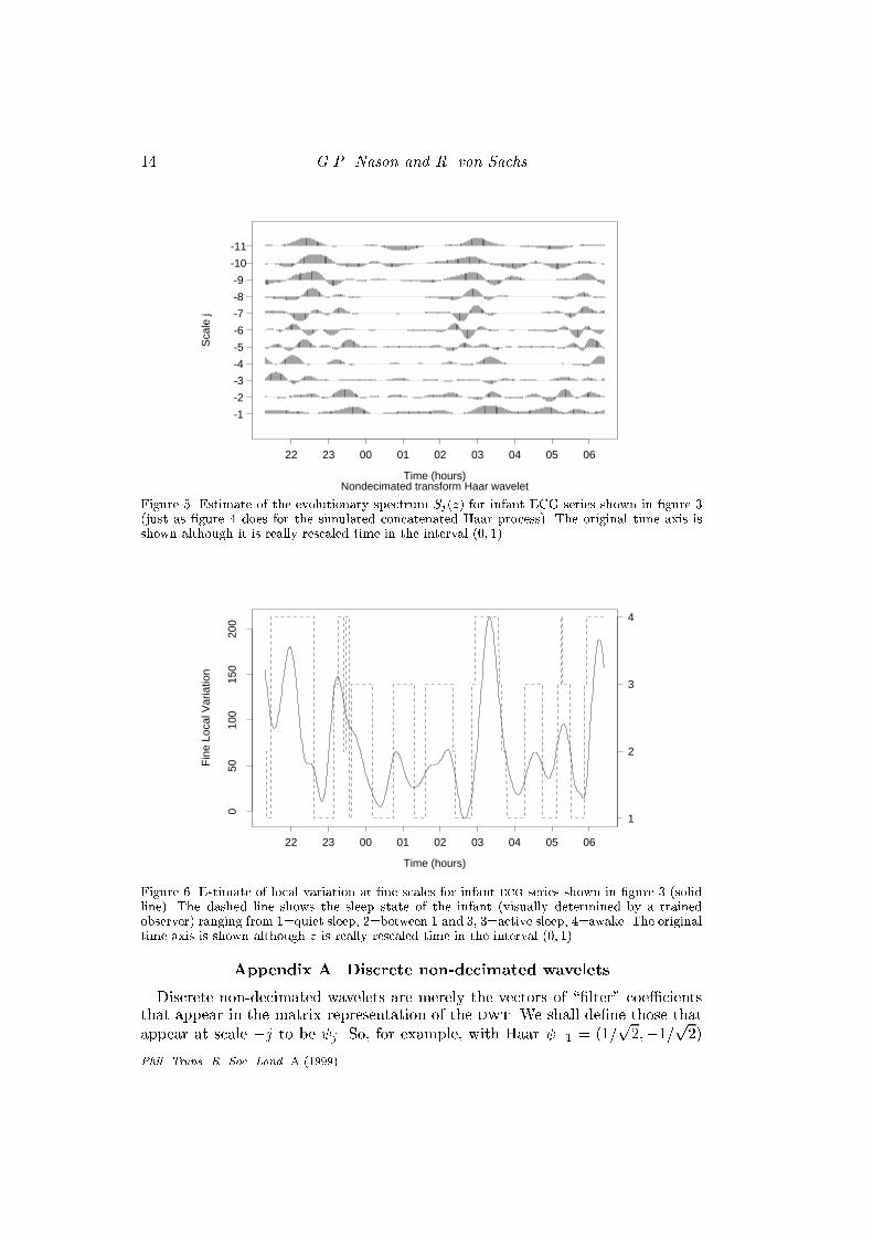
Figure 5 shows an estimate of the evolutionary wavelet spectrum for the infantECG data. It can be useful to aggregate information over scales. Figure 6 displaysthe variation in the ecg series at �ne scales. The �ne scale plot was obtained bysumming over contributions from scales -1 thru -4 in the smoothed correctedwavelet periodogram (approximately 32s, 1, 2 and 4 minute time-scales). Thedashed line in �gure 6 shows another covariate: the sleep state of the infant asjudged by a trained observer. It is clear that there is a correlation between theecg and sleep state which can be exploited. There is no real clear link betweenthe sleep state and the ews at coarse and medium scales. However, a plot of anestimate of the localised variance, v, (not shown here) gives some idea of overallsleep behaviour.The ews is a useful tool in that it provides insight into the time-scale behaviour

of a time series (much in the same way as a periodogram gives information aboutpower in a stationary time series at di�erent frequencies). However, the ews hasadditional uses: Nason, Sapatinas and Sawczenko (1999) have also used the ewsto build models between sleep state (expensive and intrusive to measure) andecg (cheap and easy) which allows estimates of future sleep state values to bepredicted from future ecg values.

We would like to thank P. Fleming, A. Sawczenko and J. Young of the Institute of Child Health,Royal Hospital for Sick Children, Bristol for supplying the ecg data. Nason was supported inpart by EPSRC Grants GR/K70236 and GR/M10229 and von Sachs by DFG Grant Sa 474/3-1and by EPSRC Visiting Fellowship GR/L52673.



Nondecimated transform Haar waveletTime (hours)

Sca

le j

-1

-2

-3

-4

-5

-6

-7

-8

-9

-10

-11

22 23 00 01 02 03 04 05 06

Figure 5. Estimate of the evolutionary spectrum Sj(z) for infant ECG series shown in �gure 3(just as �gure 4 does for the simulated concatenated Haar process). The original time axis isshown although it is really rescaled time in the interval (0; 1).

Time (hours)

Fin

e Lo

cal V

aria

tion

050

100

150

200

22 23 00 01 02 03 04 05 06

1

2

3

4

Figure 6. Estimate of local variation at �ne scales for infant ecg series shown in �gure 3 (solidline). The dashed line shows the sleep state of the infant (visually determined by a trainedobserver) ranging from 1=quiet sleep, 2=between 1 and 3, 3=active sleep, 4=awake. The originaltime axis is shown although z is really rescaled time in the interval (0; 1).

Appendix A. Discrete non-decimated wavelets

Discrete non-decimated wavelets are merely the vectors of \�lter" coe�cientsthat appear in the matrix representation of the dwt. We shall de�ne those thatappear at scale �j to be j . So, for example, with Haar �1 = (1=

p2;�1=p2)



and �2 = (1=2; 1=2;�1=2;�1=2) and so on for other scales. The j for j =�1; : : : ;�J can be obtained for any Daubechies compactly supported waveletusing the formulae:

~hj�1;n =Xk

hn�2k~hj;k; j;n =Xk

gn�2k~hj;k

where fhkg and fgkg are the usual Daubechies quadrature mirror �lters and~h�1;k = hk. For non-decimated wavelets jk(�) is the kth element of the vector j(k��), i.e. jk shifted by integers � . The key point for non-decimated discrete

wavelets is they can be shifted to any location and not just by shifts by 2�j (asin the dwt). Hence non-decimated discrete wavelets are no longer orthogonalbut an overcomplete collection of shifted vectors. The ndwt can be computedthrough a fast algorithm (similar to the Mallat pyramid algorithm described inSilverman, 1999) which takes a computational e�ort of order n log n for a dataset of length n. See Nason and Silverman (1995) for a more detailed descriptionof the ndwt.

References

Abry, P. Flandrin, P., Taqqu, M. & Veitch, D. 1999 Wavelets for the analysis, estimation andsynthesis of scaling data. in: Self Similar Network Tra�c Analysis and Performance Evalua-tion. (eds. K. Park and W. Willinger). Wiley.

Abry, P., Gon�calv�es, P. & Flandrin, P. 1995 Wavelets, spectrum analysis and 1/f processes.In Wavelets and Statistics (ed. A. Antoniadis & G. Oppenheim). Springer Lecture Notes inStatistics, no. 103, pp. 15{29.

Allan, D.W. 1966 Statistics of atomic frequency clocks. Proceedings of the IEEE, 31, 221{230.

Beran, J. 1994 Statistics for long-memory processes. London: Chapman and Hall.

Coifman, R. R. & Donoho, D. L. 1994 Translation-invariant denoising. InWavelets and Statistics(ed. A. Antoniadis & G. Oppenheim). Springer Lecture Notes in Statistics, no. 103, pp. 125{150.

Dahlhaus, R. 1997 Fitting time series models to nonstationary processes. Ann. Statist. 25, 1{37.

Donoho, D. L., Johnstone, I. M., Kerkyacharian, G. & Picard, D. 1995 Wavelet shrinkage:Asymptopia? (with discussion). J. Roy. Statist. Soc. B57, 301{369.

Farge, M. 1999 Intermittency and coherent votices in fully-developed turbulence. Phil. Trans.R. Soc. Lond. A 357 (to appear).

Flandrin, P. 1998. Time{Frequency / Time{Scale Analysis (Wavelet Analysis and Its Applica-tions, Vol 10). Academic Press, San Diego, CA.

Gao, H.-Ye 1997. Choice of thresholds for wavelet shrinkage estimate of the spectrum. J. TimeSeries Anal., 18, 231{251.

Gon�calv�es, P. & Flandrin, P. 1993 Bilinear Time-Scale Analysis Applied to Local Scaling Ex-ponents Estimation. in: Progress in Wavelet Analysis and Applications (Y. Meyer and S.Roques, eds.), pp. 271{276, Editions Frontieres, Gif-sur-Yvette.

Johnstone, I.M. 1999 Wavelets and the theory of nonparametric function estimation. Phil. Trans.R. Soc. Lond. A 357 (to appear).

Ho�mann, M. 1999. On nonparametric estimation in nonlinear AR(1)-models. Statistics andprobability letters (to appear).

McCoy, E.J. & Walden, A.T. 1996 Wavelet analysis and synthesis of stationary long-memoryprocesses. Journal of Computational and Graphical Statistics, 5, 26{56.

Nason, G.P., Sapatinas, T. & Sawczenko, A. 1999 Statistical modelling of time series usingnon-decimated wavelet representations. Preprint, University of Bristol.



Nason, G. P. & Silverman, B. W. 1995 The stationary wavelet transform and some statisti-cal applications. In Wavelets and Statistics (ed. A. Antoniadis & G. Oppenheim). SpringerLecture Notes in Statistics, no. 103, pp. 281{300.

Nason, G.P., von Sachs, R. & Kroisandt, G. 1998 Wavelet processes and adaptive estimationof the evolutionary wavelet spectrum. Discussion Paper 98/22, Institut de Statistique, UCL,Louvain-la-Neuve.

Neumann, M. 1996. Spectral density estimation via nonlinear wavelet methods for stationarynon-Gaussian time series. J. Time Ser. Anal., 17, 601{633.

Neumann, M. & von Sachs, R. 1997. Wavelet thresholding in anisotropic function classes andapplication to adaptive estimation of evolutionary spectra. Ann. Statist., 25, 38{76.

Page, C.H. 1952 Instantaneous power spectra. J. Appl. Phys. , 23, 103{106.

Percival, D.B. & Guttorp, P. 1994 Long-memory processes, the Allan variance and wavelets.In Wavelets in Geophysics (ed. E. Foufoula-Georgiou & P. Kumar), pp. 325{344, AcademicPress.

Priestley, M.B. 1965 Evolutionary spectra and non-stationary processes. J. Roy. Statist. Soc. B27, 204{237.

Priestley, M.B. 1981 Spectral Analysis and Time Series. London: Academic Press.

Rioul, O. & Vetterli, M. 1991 Wavelets and signal processing. IEEE Sig. Proc. Mag., 8, 14{38.

Serroukh, A., Walden, A.T. & Percival, D.B. 1998 Statistical properties of the wavelet varianceestimator for non-Gaussian/non-linear time series. Statistics Section Technical Report, TR-98-03. Department of Mathematics, Imperial College, London.

von Sachs, R. & MacGibbon B. 1998 Nonparametric curve estimation by wavelet thresholdingwith locally stationary errors (submitted for publication).

von Sachs, R. & Neumann, M. 1998 A wavelet-based test for stationarity (submitted for publi-cation).

von Sachs, R. & Schneider, K. 1996 Wavelet smoothing of evolutionary spectra by non-linearthresholding. Appl Comp. Harmonic Anal. , 3, 268{282.

Silverman, B.W. 1999 Wavelets in statistics: beyond the standard assumptions. Phil. Trans. R.Soc. Lond. A 357 (to appear).

Silverman, R.A. 1957 Locally stationary random processes. IRE Trans. Information Theory,IT-3, 182{187.

Wang, Y., Cavanaugh, J. and Song, Ch. 1997 Self-similarity index estimation via wavelets forlocally self-similar processes. Preprint, Dept. Stat., University of Missouri.

Whitcher, B., Byers, S.D., Guttorp, P. & Percival, D.B. 1998 Testing for homogeneity of variancein time series: long memory, wavelets and the Nile river. Submitted for publication.

Wornell, G.W. and Oppenheim, A.V. 1992 Estimation of fractal signals from noisy measurementsusing wavelets. IEEE Transactions on signal processing, 40, 611{623.


elets - university of bristolmagpn/research/papers/roysoc.pdf · w a v elets in time series...

Documents