electronic voting and social spending: the impact of

University of Brasilia

Economics and Politics Research Group

A CNPq-Brazil Research Group

http://www.EconPolRG.wordpress.com

Research Center on Economics and FinanceCIEF

Research Center on Market Regulation–CERME

Research Laboratory on Political Behavior, Institutions

and Public PolicyLAPCIPP

Master’s Program in Public EconomicsMESP

Electronic voting and Social Spending: The impact of

enfranchisement on municipal public spending in Brazil

Rodrigo Schneider, Diloá Athias and Maurício Bugarin

University of Illinois at Urbana-Champaign and UnB

Economics and Politics Working Paper 62/2016 January 13th, 2016

Economics and Politics Research Group Working Paper Series

http://www.econpolrg.wordpress.com/

1

Electronic voting and Social Spending:

The impact of enfranchisement on municipal public spending in Brazil

Rodrigo Schneiderμ Diloá Athiasδ Mauricio Bugarinσ

Abstract

This article studies the effect of voting enfranchisement focused on the poor in Brazil and its

consequences on municipal level social public spending. According to the model constructed in

this work, it should be expected an increase in social spending. This prediction is empirically

tested using electronic voting (EV) as instrument since it has impacted positively voting

enfranchisement, biased toward the poor voter, without having a direct effect on public spending.

A 2SLS regression and a differences-in-differences methodology are both applied to show that

municipalities that used EV spent more on health, education and public employment compared to

the ones that didn’t confirming the hypothesis presented in our model.

Key words: Electronic voting; political participation; politically motivated intergovernmental

transfers; social public spending.

μ Department of Economics, University of Illinois at Urbana-Champaign, 1407 W. Gregory Dr., 214 David Kinley Hall - Urbana, Illinois 61801, e-mail: [email protected]. δ Department of Economics, University of Illinois at Urbana-Champaign, 1407 W. Gregory Dr., 214 David Kinley Hall - Urbana, Illinois 61801, e-mail: [email protected]. σ Department of Economics, University of Brasilia, Campus Darcy Ribeiro, ICC Norte, Asa Norte, CEP 70910-900, Brasília, DF, Brazil, e-mail: [email protected].

mailto:[email protected]



2

1- Introduction

Brazilian redemocratization in the 1990s has significantly increased its government role

as a public goods’ provider. Part of this phenomenon can be explained by voter enfranchisement

biased towards the poor and less educated. The introduction of the electronic voting (EV) system

has helped illiterates (or functional illiterates) to cast their votes without affecting educated

citizens for which reading the instructions and filling a ballot was a trivial task. Therefore, even

though the turnout remained closely the same, the income of the median voter that can actually

cast a vote has decreased due to EV, making redistributive policies more likely to be supported.

The discussion about voters’ demands has an earlier tradition. Alexis de Tocqueville in

his seminal book “Democracy in America” argued that allowing those who do not own property

to vote, would increase the proportion of voters who are in favor of income redistribution.

Theoretical models have also predicted that an increase in voting participation of poorer voters is

positively related to an increase in social spending (Meltzer & Richards (1981), Bugarin &

Portugal (2015)). Meltzer & Richards (1983) attempt to confirm empirically their own model

prediction. However, by using the income of the median income earner as a proxy for the income

of the median voter, they did not take into account that voter turnout is low for the poor. One

would make the same mistake in the Brazilian case before the EV introduction because the

income of the median voter was smaller than the income of the median voter who could correctly

cast a vote.

There are other empirical works confirming Meltzer & Richards (1981) prediction

(Lindert (2004), Mueller and Stratmann (2003), Oliveira (2005)). Nonetheless, it has remained a

challenge to find an identification strategy to solve the reverse causality problem of regressing

directly government spending on voting participation. The more the government spends, the

3

more likely poor people will participate in the elections to keep the status quo. The present work

solves the reverse causality problem and answer the question of how does an increase in political

participation or voters’ enfranchisement affects government spending.

Although an increase in voting participation in Brazil was expected right after the

redemocratization,1 this was not observed. The high turnout before EV was not reflected in a

large number of votes being cast, especially for Representatives that didn’t have their names

printed in the ballot. The proportional representation system imposes each one of the 27

Brazilian states to act as a multi-member district holding at least 8 and at most 70 seats in

congress (lower chamber). As a consequence, the pool of Federal Representatives’ candidates to

be chosen by a voter is large (this is also the case for State Representatives) making it

impractical to print all their names in a ballot so the voter, before EV, had to actually write in a

specific blank space on the ballot their candidate’s name or respective number in order to cast a

valid vote for him (or her). That way, knowing how to read and clearly write was essential to cast

a vote. As pointed by Hidalgo (2010), for a country with an electorate’s illiteracy rate close to a

third, this wasn’t a trivial task.

The consolidation of Brazilian democracy, therefore, came with the introduction of

electronic voting (EV), which has allowed voters, mainly the poor, to exercise their right to vote

(Schneider 2015). The EV was introduced in Brazil in order to make voting easier to all citizens

and consequently increase the power of the Brazilian democracy. For instance, in the 1994

elections, before EV, the valid vote to turnout ratio for Federal Representatives was only 58%.

1 The new constitution of 1988 has granted to all eligible voters the right of a direct, secret, universal and periodic vote. Also, in Brazil voting is mandatory which can help to explain its high turnout of 80% on average.

4

While in 2002, when EV was already being used in all polling stations in the country this number

increased to 92% according to the Supreme Electoral Court, TSE.

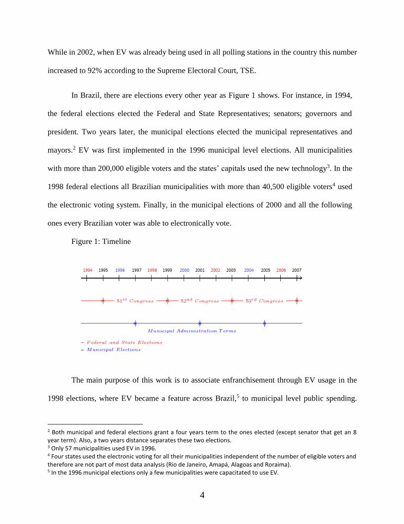
In Brazil, there are elections every other year as Figure 1 shows. For instance, in 1994,

the federal elections elected the Federal and State Representatives; senators; governors and

president. Two years later, the municipal elections elected the municipal representatives and

mayors.2 EV was first implemented in the 1996 municipal level elections. All municipalities

with more than 200,000 eligible voters and the states’ capitals used the new technology3. In the

1998 federal elections all Brazilian municipalities with more than 40,500 eligible voters4 used

the electronic voting system. Finally, in the municipal elections of 2000 and all the following

ones every Brazilian voter was able to electronically vote.

Figure 1: Timeline

The main purpose of this work is to associate enfranchisement through EV usage in the

1998 elections, where EV became a feature across Brazil,5 to municipal level public spending.

2 Both municipal and federal elections grant a four years term to the ones elected (except senator that get an 8 year term). Also, a two years distance separates these two elections. 3 Only 57 municipalities used EV in 1996. 4 Four states used the electronic voting for all their municipalities independent of the number of eligible voters and therefore are not part of most data analysis (Rio de Janeiro, Amapá, Alagoas and Roraima). 5 In the 1996 municipal elections only a few municipalities were capacitated to use EV.

5

Therefore, EV is used as an instrument to show how change in enfranchisement (or number of

correctly cast votes) affects social spending at the municipal level. The connection between the

federal and municipal election is established taking into account how mayors respond to the

federal elections in the middle of their terms in office: In order to get reelected,6 the mayor which

municipality used EV in 1998, is going to respond to the poor voter enfranchisement by

increasing public spending.7 At the same time, Representatives elected in 1998 will be willing to

help mayors from municipalities that used EV through intergovernmental transfers, mostly used

in social spending, in exchange for support in the next federal elections as these mayors can now

deliver more votes to them. As argued by Novaes (2015), in multi-member districts (Brazilian

case), mayors are important brokers for Representatives.

This result should be expected due to the intuition provided by our model, similar to the

one constructed by Bugarin & Portugal (2015), which concludes that the optimum amount of

public provision is biased toward the preferred policy of the socioeconomic class with higher

turnout. The difference is that in our model all voters are necessarily going to show up to vote,

since voting is mandatory in Brazil. However, they may not correctly cast their votes.

Interestingly, since the EV is not only going to enfranchise voters but it is also going to bias this

enfranchisement disproportionately towards the poor, as showed in previous econometric works

(Fujiwara, 2015; and Schneider, 2015), the model is going to predict that the provision of public

goods should therefore increase because the poor are the ones more likely to demand public

goods and at the same time, to be de facto enfranchised.

6 All mayors were able to try reelection in 2000 since the law granting mayor the possibility for reelection started being effective in 1997, one year after the mayoral election of 1996. 7 Since the Federal elections took place in 1998, the mayor was able to respond to it for two years before trying reelection in the municipal elections of 2000.

6

Besides presenting a model to motivate the empirical analysis, this work is going to rely

on two econometric methodologies. Assuming the 1998 municipalities’ assignment for EV usage

as good as random, this work first estimates a two stage least square regression (using as

dependent variable the logarithm of the social public spending) in order to measure the

enfranchisement impact on government spending at the municipal level during the last two years

of mayoral four years’ term (1999 and 2000). EV assignment is used as instrument as it affects

valid votes to turnout ratio for representatives without directly affecting social spending. To

guarantee that EV usage is the only difference between the compared municipalities, the analysis

will be restrained to places where the number of eligible voters is close to 40,500. Municipalities

near this cutoff have similar characteristics and vote preferences and any differences between

them are given by EV usage only. As municipalities that used EV had an increase on valid votes

to turnout ratio close to 20 p.p. and 15 p.p. respectively for federal and state representatives

(Fujiwara 2015, Hidalgo, 2010, Schneider, 2015), it should be expected a disproportionately

higher amount of public provision in these places.

Secondly, in order to collect a larger sample, as most municipalities (92.3%) had less

than 40,500 voters in 1998, a difference-in-differences analysis, taking into account these places,

is going to be constructed. To use this methodology, four states that had EV in all their territories

are going to be used as the treatment group and the remaining ones will be the control. Our focus

will be only on municipalities with less than 40,500 voters in order to avoid heterogeneity

between the two groups. The EV’s impact on government spending will be found by comparing

the differences between the amount of public expenditure on the treatment and control group

before the EV usage (last two years of the mayoral term that ended in 1996) and after it (last two

7

years of the mayoral term that ended in 2000). It should be expected a much larger and

significant public spending increase on the municipalities that used EV in 1998.

Besides the introduction, this work is divided as follows: Section 2 presents a literature

review on the connection between voting participation and public spending and discusses the EV

implementation. Section 3 presents a model to motivate the empirical analysis. Section 4 briefly

discusses the data collection. Section 5 presents the 2SLS model and Section 6 the differences-

in-differences. Finally, section 7 concludes the work.

2- Background

2.1. Voters’ enfranchisement and public spending

Meltzer & Richard (1981) show that voting enfranchisement increases public spending.

Using a model of electoral competition, they argue that the median income voter is the one

imposing his (or her) preferences on public spending. Moreover, the electoral equilibrium shows

that: the poorer the median income voter is, the larger will be his (or her) public spending

optimum provision demanded. This result comes from the fact that, the poorer the citizen is, the

lower will be his (or her) tax contribution to finance the public provision. Lindert (2004)

developed an econometric study using decennial data from OECD countries between 1880 and

1930 to confirm the positive relationship between government size and vote participation. In

Latin America, Brown & Hunter (1999) study the relationship between democracy and public

social spending using panel data for 17 countries between 1980 and 1992. The authors’ conclude

that, especially in poor and economic instable countries, democracy increases the allocation of

public spending on social programs when compared to dictatorship regimes.

8

For the United States, Husted & Kenny (1997) make a panel data analysis for 46

American states between 1950 and 1988. During this period, restrictions to vote focused mainly

on the poor, such as poll taxes payments and literacy tests, were banned in the country increasing

voting participation and, at the same time, decreasing the income of the median voter. Therefore,

it should come as no surprise the result found on their study showing that a reduction of 0.2 on

the median voter income to the total population income ratio caused an increase of 5 to 12% on

public social spending.

Besides the empirical evidence mentioned above, Meltzer & Richard (1981) argument is

not consensual. Alesina & Giuliano (2009), for instance, argue that the empirical studies are

limited and other aspects such as median voter’s social mobility perspective and strength of

lobbying groups could reinforce the limits imposed on government intervention in the economy.

A possible way to explain the difficulty to find empirical evidence on the relationship between

the median’s voter income and public spending is given by the fact that the median income of the

citizen may not be the same as the median income of those who actually showed up to vote. That

is, even if the democracy allows all eligible voters to cast their votes, those who don’t vote have

their preferences completely ignored. As Mueller & Stratmann (2003) show, there is a positive

relationship between turnout and public spending.

Therefore, democracy by itself is not enough to guarantee larger public spending.

According to UNDP (2005), between 1990 and 2002, less than 55% of all eligible voters living

in a democracy showed up to vote and cast a vote to a candidate (or party). More importantly,

those abstaining to vote are more likely to represent the poor (and illiterates). Frey (1971) shows

a positive relationship between income and electoral participation in the United States. Greene &

Nikolaev (1999) using electoral polls between 1972 and 1993 concluded that electoral

9

participation monotonically increases with income. Borgonivi et al. (2010) show a positive

relationship between education and electoral participation in 15 European countries. In Brazil,

Elkins (2000) finds a positive relationship between political concern and education.

Consequently, a lower political participation concentrated on the poor makes the median

voter income to be larger than the median citizen income reducing the preferences for public

goods given by the electoral equilibrium as argued by Bugarin & Portugal (2015). A solution

pointed by these authors is to use mandatory voting.8 Jackman (2001) uses the Australia

elections to show how mandatory voting increase voting participation (the turnout has increased

from 65% to 95% after mandatory voting was imposed in this country). However, mandatory

voting by itself cannot guarantee voting participation. As aforementioned, Brazil’s case is

illustrative. Although the constitution makes it mandatory for all citizens between 18 and 70

years old to vote,9 in 1994 for instance, less than 60% of those who showed up to vote (turnout

close to 80%) could actually cast a valid vote for a candidate or party to the legislative seats.

2.2 Electronic voting and political participation in Brazil

Electronic voting (EV) was introduced in Brazil in 1996 (municipal elections). All capital

cities and municipalities with more than 200,000 voters used EV (total of 57 municipalities). In

1998 (federal elections), not only all municipalities with more than 40,500 voters have used EV,

but also all municipalities of Alagoas, Amapá, Roraima and Rio de Janeiro state (in total, 515

municipalities used). As showed in the literature (Hidalgo, 2010; Moraes, 2012; Fujiwara, 2015;

and, Schneider, 2015), EV usage is responsible for an increase of 20 p.p. in the valid votes

(correctly cast votes) to turnout ratio for federal and state representatives. As mentioned before,

8 According to The Economist (2015), 38 countries use or has used mandatory voting in their elections. 9 All Brazilian citizens, age 16 and older have the right to vote.

10

to cast a vote for representative before EV, one should clearly write the name or number of the

candidate. It could also be possible to write the name or number of the party, had the voter

decided to vote directly to the party instead of one of its representatives. Therefore, knowing

how to read in order to understand how to cast a vote and where one should specifically write the

name of the candidate in the ballot would be essential to correctly vote in Brazil.

When the new system was introduced, the voter would only need to press the candidate’s

number on a numerical keyboard (similar to a regular phone keypad commonly used in Brazil

according to Hidalgo (2010)) and after verifying the picture of the candidate one was willing to

vote for, it would be necessary to press a green button in order to cast the vote.10 The only way

one could not cast a vote, without being on purpose,11 would be to type a candidate’s number

with no correspondence to any candidate and after reading in the screen “this number is wrong”,

the voter would have to press the green button anyway. As Hidalgo (2010) points out, the EV

was considered a democratic progress since even the illiterates could press a number followed by

the green button after seeing their preferred candidates’ face on the screen.

The main four works on EV in Brazil are Hidalgo (2010), Moraes (2012), Fujiwara

(2015) and Schneider (2015). All these works converge to the fact that EV has increased political

participation.12 The last three works also show, although in different ways, that EV had a larger

impact on enfranchisement in municipalities with a larger rate of illiteracy.13 Hidalgo (2010),

focusing on federal representatives elections, shows that the party ideological choice (from left to

10 Fujiwara (2015) shows illustrations of the old ballot comparing it to the electronic one. It’s also important to notice that the government had made TV advertisement teaching how to vote in the new system and trained people to help voters if something went wrong during the voting process in the Election Day. 11 The voter could not cast a vote on purpose by pressing a white button (blank vote) followed by the green one to confirm it. 12 By increasing the valid votes to turnout ratio close to 22%. 13 Schneider (2015) also shows that EV had a larger impact on enfranchisement in municipalities with lower GDP per capita.

11

right) suffered only a small effect due to EV that benefitted the right wing parties the most. This

counter intuitive result is challenged by Schneider (2015) that taking into account regional

clientelistic relationship in Brazil, demonstrated that the left wing parties were actually the ones

disproportionately benefitted by the EV introduction.14 Moraes (2012) studies the increase in

electoral competition resulted by the EV usage and Fujiwara (2015) focuses on the public health

spending at the state level in Brazil showing that the larger the percentage of voters using EV

within a state, the larger the amount of health spending and consequently the better the health

outcomes in these places. Differently from Fujiwara (2015), our work relies on municipal level

data15 and shows that not only health, but also public employment, education and the overall

municipalities’ public expenditures increase due to EV usage. Also, this work shows that the

municipal revenue, mostly composed by federal and state transfers, of places that used EV in

1998 disproportionately increased explaining how these municipalities were able to spend more

on public goods. Therefore, this work uses a larger sample and also explains the connection

between federal representatives and mayors. Finally, it also adds to the literature by testing

empirically the predictions of the model presented in the following section.

3 – The effect of electronic vote on the electoral outcome: A political economy model

3.1 Introduction

Section 3 builds a voting model aimed at better understanding the effect of EV on the

electoral equilibrium. The model distinguishes to different stages of voters’ decision; first, a

voter decides whether or not to vote. Next, if the voter decides to vote, then she will decide to

which party to vote for.

14 The different results can be also explained by the usage of differences-in-differences and regression discontinuity design methodology by Schneider (2015) while Hidalgo (2010) uses only the former. 15 Fujiwara (2015) analyses state level data (27 observations).

12

A voter’s decision to vote is one of the most discussed issues both in Political Sciences

and in Economics as well. Indeed, considering that there is a cost associated to voting, a rational

agent will choose to vote only if she believes it is reasonably likely that her vote will change the

electoral outcome. Chamberlain & Rothschild (1981) prove that under rather general conditions,

the probability that a voter will cast the decisive vote in an election between two alternatives

(parties) in which there are 2N+1 voters is of order N-1. Therefore, in large elections the

probability of a voter being pivotal is negligible.16 But then, electoral participation should be

reduced, as also suggested in Downs (1957, p. 260-276).

However, actual electoral data show a much higher level of electoral participation, even

in countries where voting is not mandatory. For instance, the 2012 US presidential elections

showed a record low participation level of 57.4%, which is much higher than social choice

theories would predict.

Both experimental and theoretic studies aim at understanding why people vote. Blais &

Young (1999) conclude that a feeling of civic duty is a strong factor that makes people vote,

based on an experiment conducted by the Canadian Electoral Commission. Schram & Winden

(1991) present a theoretic model that also assumes the civic duty motive but adds the issue of

group identification and the fact that the larger the number of votes a group obtains, the more it

is able to affect public policy as well; it concludes that members of a group will pressure the

other members to vote. This second theoretic motive for voting is supported by Schram &

Sonnemans (1996)’s experimental study. Edlin, Gelman & Kaplan (2007) present a model in

which a citizen’s utility has a social component, i.e., she cares about the other citizens’ welfare;

16 According to John Longredan, “[…]the chances of actually influencing an election are about the same as getting hit by lightning” (in Carey, 2008).

13

she model shows that there will be higher voting participation than when a citizen has the typical

selfish utility. Harder & Kronick (2008) stresses that the social environment and the difficulties a

citizen faces to vote (due to lack of literacy, for example) affect the willingness to vote. Finally,

Feddersen & Sandroni (2006)’s model assumes that citizens care about the aggregate social cost

of voting and introduces the concept of “ethical rules” that determine which citizens will vote in

equilibrium; that model endogenizes a concept similar to the exogenous concept of civic duty as

part of the equilibrium solution.

In the present paper we use the concept of “willingness to vote” as a proxy for all the

motives for voting described above. In our model each citizen 𝑖 has a willingness to vote 𝜈𝑖 ∈

𝑉 ⊂ ℝ+. The willingness 𝜈𝑖 ≥ 0 represents the utility gain agent 𝑖 receives when he votes,

regardless of the final result of the election. Note that, since the citizen understand that his vote

insignificant, his decision on whether or not to vote depends on the comparison between the cost

of voting and his willingness to vote. If the cost is lower than the willingness to vote, the agent

will then decide to participate and will vote sincerely, for the party that better represents his

preferences.

Hence, our electoral analysis will be divided in two steps. In the first step, each citizen

decides whether or not to vote, based on her cost to vote and on her willingness to vote. In the

second step, those who decided to vote take their ballots.

3.2. First step: The decision to vote

Primitives of the model

There is a continuum of agents of mass 1, 𝑊 = [0,1]. Each agent 𝑖 ∈ 𝑊 has a type 𝜈𝑖 ∈

𝑉 ⊂ ℝ+, his willingness to vote. In particular, if 𝜈𝑖 = 0, then agent 𝑖 sees no value in voting. The

14

willingness to vote 𝜈𝑖 is a continuous random variable distributed in a non-negative set 𝑉

according to the distribution 𝐹(𝜈𝑖).

If he decides to vote, citizen 𝑖 will incur a cost 𝜅𝑖 ∈ ℝ+. The cost reflects a number of

components. Directly, it reflects the displacement costs, the opportunity cost of time, etc. Most

importantly, it reflects the cost of gathering the information he needs in order to decide who to

vote for, as well as preparing for filling properly the complex voting cell. That is the component

that will matter in the present model, since that component may change according to the voting

technology, as discussed previously.

General electoral participation

An agent of type 𝜈𝑖 and cost 𝜅𝑖 will decide to vote if and only if:

𝜈𝑖 − 𝜅𝑖 ≥ 0. (1)

Let 𝐸 = {𝑖 ∈ 𝑊| 𝜈𝑖 − 𝜅𝑖 ≥ 0} be the set of voting citizens. Then the cardinality of 𝐸, |𝐸|,

corresponds to the proportion of voting citizens. Note that the higher the expected value of the

willingness to vote, the higher the overall electoral participation, ceteris paribus. More

importantly for the present study, the lower the voting costs, the higher the proportion of voting

citizens, ceteris paribus.

An illustration of the voting costs associated to legal requirements can be found in

Brazilian institutions. Before the 1988 Brazilian Constitution voters were required to be literate

in order to vote; therefore a poorer, illiterate citizen would have to first learn how to read and

write in order to have access to voting. Similarly, before the 1960s several American States

15

required citizens to pass literacy tests in order to vote; that, in practice, reduced the vote of the

colored citizens for whom these tests were typically difficult (Husted & Kenny, 1997).

These examples suggest that poorer citizens tend to have lower electoral participation.

Indeed, several empirical studies suggest that this is indeed the case, as reviewed in Bugarin &

Portugal (2015). In what follows we include such a friction in the original model.

Different electoral participation by social classes

Suppose now that society is divided in three income classes. The low-income class P is

formed of poorer citizens with income 𝑦𝑃. The middle-income class M congregates the middle

class with income 𝑦𝑀 and the high-income class R is composed of richer citizens with income

𝑦𝑅, where 𝑦𝑃 < 𝑦𝑀 < 𝑦𝑅. A class 𝐽 = 𝑃, 𝑀, 𝑅 has mas 𝛼𝐽 ∈ [0,1] where 𝛼𝑃 + 𝛼𝑀 + 𝛼𝑅 = 1.

Suppose now that there is total orthogonality between income and willingness to vote, so

that the willingness to vote is distributed in each class according to the same distribution function

𝐹(𝜈𝑖). Furthermore, suppose for simplicity that the all citizens sharing the same income class

share the same voting cost, i.e., 𝜅𝑖 = 𝜅𝐽 for every citizen 𝑖 class 𝐽, 𝐽 = 𝑃, 𝑀, 𝑅. Finally, as

discussed before, suppose that the cost of voting is higher for the low-income class, i.e., 𝜅𝑃 >

𝜅𝑀, 𝜅𝑅 .

Therefore, 𝐹(𝜅𝐽) corresponds to the percentage of citizens from class 𝐽 = 𝑃, 𝑀, 𝑅 that

gives up voting. Hence, 𝛼′𝐽 = [1 − 𝐹(𝜅𝐽)]𝛼𝐽 is the percentage of citizens that belong to class 𝐽

and vote, 𝜂𝐽 = 𝐹(𝜅𝐽)𝛼𝐽 is the percentage of citizens that belong to class 𝐽 and do not vote, and

𝛼𝐽 = 𝛼′𝐽 + 𝜂𝐽.

The effect of the electronic vote on each class’ electoral participation

16

Our model allows us to investigate the effect of the electronic vote on the each income

class. Suppose that class P, besides being the poorer class, is also the class with lowest literacy

levels, so that, it is also the class with highest voting costs with the older voting technology,

because it requires memorizing and writing down the candidates’ names, as discussed earlier.

Then, the percentage of electoral participation will be lower in class P (𝜅𝑃 > 𝜅𝑀, 𝜅𝑅 → 1 −

𝐹(𝜅𝑃) < 1 − 𝐹(𝜅𝑀), 1 − 𝐹(𝜅𝑅)).

What would be the effect of implementing EV? We expect that the EV will create the

highest changes precisely in class P that has the highest rate of illiteracy. In that class, the easier

voting technology will reduce voting costs, from 𝜅𝑃 to �̃�𝑃 < 𝜅𝑃. As for the other classes, that

includes citizens better able to read and write and with higher education levels, the effect of EV

will be less significant. Hence, for simplicity we assume that EV does not affect the voting costs

for the other two classes. Therefore, EV will allow higher participation rates for the poor class

without significantly changing the participation rates in the remaining classes.

3.3. Second step: Electoral equilibrium with heterogeneous participation

The basic ideas of the model

The electoral competition model presented here follows Bugarin & Portugal (2015). Two

parties simultaneously announce political platforms. A platform consists of a provision of a

public good that will be produced if the party wins the election. Production of the public good is

totally funded by taxes to be collected from every citizen according to a single tax rate. Since

society is composed of three income classes, all citizens from the same class will have the same

preferences for public good provision. Furthermore, since all citizens benefit the same way from

17

public good consumption but the poorer ones pay fewer taxes for its production, typically the

poorer classes prefer more public goods than the rich ones.

A number of citizens in each class do not vote. Those who vote will vote sincerely, for

the party that better represents his preferences. Citizens’ preferences take into consideration

parties’ platforms but are also influenced by unpredicted stochastic factors that are orthogonal to

the announced platforms. Examples of such factors are sexual scandals or a terrorist attack,

among others.

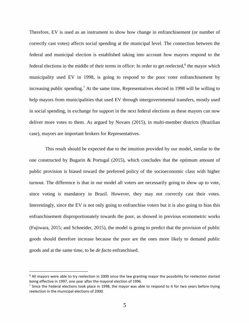
Elections are held in one national electoral district in which each voter has one vote.

After the elections, each party is assigned a quantity of seats in the Legislature that corresponds

to the percentage of votes it received. After the new Legislature is formed, the party that has a

majority of seats (we assume an odd number of seats) implements its campaign platform: taxes

are collected and the public good is provided. Figure 1 presents the general form of the game.

Note that only the first and the third boxes correspond to agents’ decisions. Furthermore,

decisions in the third box are straightforward since voting citizens vote sincerely. The details of

the electoral competition game and its solution are presented next.

Figure 2 - The electoral competition game

Parties

announce

their

political

platforms

Stochastic

shocks

affecting

voters’

preferences

are realized

Voting

citizens

take

their

ballots

The

victorious

party

implements

its platform

18

The electoral completion game with heterogeneous participation17

Society is composed of three income classes, as previously described. Two parties P=A, B

announce simultaneously a per capita level of provision of a public good, 𝑔𝐽, 𝐽 = 𝐴, 𝐵, to be

implemented by the winning party. Public good production is financed by an income tax

collected according to the tax rate 𝜏, common to all agents. All tax-collected resources are used

for the public good’s provision. Then the government budget constraint is given by the equation

below, where ∑ (𝜂𝐽 + 𝛼′𝐽)𝐽 𝑦𝐽 = ∑ 𝛼𝐽𝐽 𝑦𝐽 = 𝑦 represents the average income of all citizens.

𝜏 ∑ (𝜂𝐽 + 𝛼′𝐽)𝐽 𝑦𝐽 = 𝜏𝑦 = 𝑔 (2)

A voter’s utility has two components: a pragmatic component and an ideological one. This

is the most general way of characterizing an economic agent who also has political concerns; for

more on this topic, see Ferejohn (1986), Bugarin (1999) and Bugarin (2003). The pragmatic or

economic part of the utility represents the voter’s decisions as a homo œconomicus and depends

on the consumption of a private good, as well as the consumption of the public good. Thus, if a

citizen of class 𝐽 has private consumption 𝑐𝐽 and public good consumption 𝑔, its utility is 𝑐𝐽 +

𝐻(𝑔) where 𝐻 is a twice differentiable, strictly increasing, and strictly concave function. In the

present model public good provision and the corresponding income tax rate are the result of the

electoral process; therefore, the homo œconomicus will choose the highest possible private

consumption, i.e., 𝑐𝐽 = (1 − 𝜏)𝑦𝐽, and the resulting pragmatic component of his utility is:

(1 − 𝜏)𝑦𝐽 + 𝐻(𝑔). (3)

17 This section and the following section as well draw heavily on Bugarin & Portugal (2015).

19

Hence, we can write that agent’s pragmatic utility as 𝑊𝐽(𝑔) = (𝑦 − 𝑔)𝑦𝐽

𝑦+ 𝐻(𝑔).

Therefore, his preferred public policy is:

𝑔∗𝐽 = (𝐻′)−1 (𝑦𝐽

𝑦) , 𝐽 = 𝑃, 𝑀, 𝑅. (4)

Note that 𝑔∗𝑃 > 𝑔∗𝑀 > 𝑔∗𝑅, i.e., the poorer a citizen is, the more favorable he is to public

expenditure, as discussed before. This result is well known in the literature and has been

carefully formalized in Meltzer & Richard (1981). It explains the increase in the size of

governments throughout the 19th and 20th centuries as a consequence of the expansion of

suffrage in the consolidating western democracies.

The ideological component of a voter’s utility function reflects his concerns as a homo

politicus and depends on two random variables corresponding to the voter’s bias towards party

B, or equivalently, party B’s popularity at the time the election is held18. The first random

variable is common to all voters and relates to the realization of a state of nature that affects the

entire population. A war, an abrupt change in international oil prices and a countrywide energy

crisis are examples of such phenomena. A clear example is the popularity of the U.S. president

after the terrorist attack on September 11th, 2001, which increased from 57% in February to 90%

in September.19 We model that process with a random variable 𝛿 uniformly distributed on

[−1

2𝜓,

1

2𝜓]. The parameter >0 measures the level of sensibility of society to these shocks: the

lower the value of , the more those shocks may affect society. To illustrate, price changes in oil

may strongly affect the political equilibrium in a country that depends strongly on that product,

18 Analogous results would obtain if we had set the bias with respect to party A due to the symmetry of the bias. 19 See “Poll Analyses”, Section “Gallup Poll News Service”, The Gallup Organization, http:/www.gallup.com, 09/24/2001.

20

such as Venezuela, and have much less effect in countries that produce near their internal

demand levels, such as Brazil.

The second random variable is particular to each voter i in group 𝐽 and reflects his personal

bias towards party 𝐵. It relates to information about relevant politicians on issues that are not

consensual in society, such as release of information that a candidate used drugs in his youth;

some voters may believe that this fact makes him unsuitable to a political leadership career,

others may find no relation whatsoever with his political career, others may even sympathize

with the candidate. We model that bias as a random variable 𝜎𝑖𝐽 uniformly distributed on

[−1

2𝜙,

1

2𝜙]. Hence, the greater the parameter 𝜙, the more homogeneous class 𝐽 is.

Therefore, if party B wins a majority of seats in the Legislature with platform 𝑔𝐵, voter i in

the social class 𝐽 derives utility:

𝑊𝐽(𝑔𝐵) + 𝜎𝑖𝐽 + 𝛿. (5)

Note that it may be the case that the realization of 𝛿 is positive whereas the realized value

of 𝜎𝑖𝐽is negative. Suppose, for example, that the GDP of country increases above expectations,

which brings about overall support for the incumbent president’s party, but the media releases

the news of a sexual scandal in the presidential office, which may affect different voters in

different ways.

The solution to the electoral competition game

We solve the game by backwards induction. Suppose party P announces policy 𝑔𝑃, P = A,

B. Then, voter 𝑖 in class 𝐽 prefers party A to party B if and only if:

21

𝑊𝐽(𝑔𝐴) > 𝑊𝐽(𝑔𝐵) + 𝜎𝑖𝐽 + 𝛿. (6)

Then, the voter that is exactly indifferent between the two parties in class 𝐽 corresponds to

the realization 𝜎𝐽 of the random variable 𝜎𝑖𝐽 given by the following equation 𝜎𝐽 = 𝑊𝐽(𝑔𝐴) −

𝑊𝐽(𝑔𝐵) − 𝛿.

Since citizens vote sincerely, the number of votes party A receives is:

𝜋𝐴 = ∑ 𝛼′𝐽 ∙ Prob𝐽 [𝜎𝑖𝐽 ≤ 𝜎𝐽] = ∑ 𝛼′𝐽𝐽 [𝜎𝐽 +

1

2𝜙] 𝜙 = ∑ 𝛼′𝐽𝜎𝐽𝜙 +

𝛼′

2𝐽 . (7)

Define 𝑊′(𝑔𝐴) = ∑ 𝛼′𝐽𝐽 𝑊𝐽(𝑔𝐴) and 𝑊′(𝑔𝐵) = ∑ 𝛼′𝐽

𝐽 𝑊𝐽(𝑔𝐵). Then the probability of

victory of party A is:

𝑝𝐴 = Prob [𝜋𝐴 ≥𝛼′

2] = Prob [𝛿 ≤

1

𝛼′[𝑊′(𝑔𝐴) − 𝑊′(𝑔𝐵)]]. (8)

The above expression can be rewritten as:

𝑝𝐴 =1

2+

𝜓

𝛼′[𝑊′(𝑔𝐴) − 𝑊′(𝑔𝐵)]. (9)

By symmetry, the probability of victory of party B is:

𝑝𝐵 =1

2−

𝜓

𝛼′[𝑊′(𝑔𝐴) − 𝑊′(𝑔𝐵)]. (10)

Parties choose their announced platforms in order to maximize their probability of winning

the election given by (9) and (10). Therefore, party A solves the following problem:

max𝑔𝐴

𝑝𝐴(𝑔𝐴, 𝑔𝐵) =1

2+

𝜓

𝛼′[𝑊′(𝑔𝐴) − 𝑊′(𝑔𝐵)] (11)

Subject to: 0 ≤ 𝑔𝐴 ≤ 𝑦.

22

Moreover, party B solves a completely similar problem. The solution to this platform

announcement simultaneous game yields the same dominant strategy to both parties, given

below, where 𝑦′ =∑ 𝛼′𝐽

𝐽 𝑦𝐽

∑ 𝛼′𝐽𝐽

=∑ 𝛼′𝐽

𝐽 𝑦𝐽

𝛼′.

𝑔𝐴 = 𝑔𝐵 = 𝑔𝐸 = (𝐻′)−1 (𝑦′

𝑦) (12)

Note that income 𝑦′ =∑ 𝛼′𝐽

𝐽 𝑦𝐽

∑ 𝛼′𝐽𝐽

=∑ 𝛼′𝐽

𝐽 𝑦𝐽

𝛼′ is a convex combination of each income class’

income, in which the weights are the percentage of citizens in each class that really vote.

Therefore, the higher the political participation in one class, the higher the weight parties give to

that class’ income and, thereby, the closer the equilibrium policy will be to that class’ preferred

policy.

For the sake of illustration, suppose that 𝛼′𝑃 = 𝛼′𝑀 = 0 and 𝛼′𝑅 > 0, i.e., only the reach

citizens vote. Then, 𝛼′ = 𝛼′𝑅, 𝑦′ = 𝑦𝑅 and 𝑔𝐸 = (𝐻′)−1 (𝑦𝑅

𝑦) = 𝑔∗𝑅, so that the platform

announced by each party is precisely the one preferred by the rich citizens. this explains again

why there was so little redistribution in the past when voting rights were restricted to land

owners.

3.4. The effect of electronic voting on the electoral equilibrium

Consider first the electoral equilibrium prior to EV. Recall that 𝛼′𝐽 = [1 − 𝐹(𝜅𝐽)]𝛼𝐽,

𝐽 = 𝑃, 𝑀, 𝑅 and 𝜅𝑃 > 𝜅𝑀, 𝜅𝑅. Then we can write (with the subscript b for “before”) as:

𝑦𝑏′ =

∑ 𝛼′𝐽𝐽 𝑦𝐽

𝛼′=

∑ [1−𝐹(𝜅𝐽)]𝛼𝐽𝐽 𝑦𝐽

𝛼′> ∑ 𝛼𝐽

𝐽 𝑦𝐽 = 𝑦. (13)

23

Since 𝛼′𝑃 < 𝛼′𝑀, 𝛼′𝑅, then it follows that 𝑔𝑎𝐸 = (𝐻′)−1 (

𝑦𝑎′

𝑦) < (𝐻′)−1(1), i.e., public

goods provision before EV is below what it would be if all citizens were voting. This is a direct

consequence of the fact that precisely the poor citizens, those who prefer more public goods

provision, are the ones who present lowest electoral participation.

Consider now the situation posterior to the introduction of EV. According to our model’s

hypotheses, 𝜅𝑀 and 𝜅𝑅 remain unchanged, whereas the cost parameter 𝜅𝑃 decreases to �̃�𝑃 < 𝜅𝑃.

Then, using the subscript a for “after”, we can write:

𝑦𝑎′ =

[1−𝐹(�̃�𝑃)]𝛼𝑃𝑦𝑃+[1−𝐹(𝜅𝑀)]𝛼𝑀𝑦𝑀+[1−𝐹(𝜅𝑅)]𝛼𝑅𝑦𝑅

[1−𝐹(�̃�𝑃)]𝛼𝑃+[1−𝐹(𝜅𝑀)]𝛼𝑀+[1−𝐹(𝜅𝑅)]𝛼𝑅 <

[1−𝐹(𝜅𝑃)]𝛼𝑃𝑦𝑃+[1−𝐹(𝜅𝑀)]𝛼𝑀𝑦𝑀+[1−𝐹(𝜅𝑅)]𝛼𝑅𝑦𝑅

[1−𝐹(𝜅𝑃)]𝛼𝑃+[1−𝐹(𝜅𝑀)]𝛼𝑀+[1−𝐹(𝜅𝑅)]𝛼𝑅 = 𝑦𝑏 ′ (14)

But then: 𝑔𝑎𝐸 = (𝐻′)−1 (

𝑦𝑎′

𝑦) > (𝐻′)−1 (

𝑦𝑏′

𝑦) = 𝑔𝑏

𝐸.

In other words, the new voting technology brings about a reduction in the cost of voting

to the poor, which increases their participation and, thereby, increases the weight of their

preferences in parties’ calculations, thereby increasing the equilibrium provision of public goods.

This is the main conclusion of the present theoretic model. The main theoretic insight is

that increasing de jure access to voting, by legally extending the suffrage to poorer citizens, is

not enough to ensure that the political parties will take these citizens’ preferences into account. It

is necessary that, in addition to having the right to vote, these citizens really exert that right. Only

in the case where poorer citizens do participate strongly in the political arena by voting, will

public policy reflect their preferences.

24

The main point of the present work is that, due to the high cost of voting to poorer,

illiterate citizens in Brazil, their preferences were not fully considered until EV technology

strongly increased their participation, changing the electoral equilibrium.

The empirical implication of the model and its testable hypotheses are straightforward: if

the model does rightfully reflect the real situation, then, we should have observed a significant

increase in the provision of public goods in Brazil after the implementation of EV. More

specifically, since poorer citizens care more about social policy (health, education, cash transfers,

etc.) we should have observed a clear increase in public spending in these areas.

The following sections test these hypotheses confirming that there was indeed a robust

increase in social expenditure in Brazil after the advent of EV and that this increase is

particularly strong in municipalities with higher numbers of illiterate citizens.

4- Data

The dependent variables are constructed using the municipal level data on public

spending available on the Brazilian National Treasury website.20 The selected topics are health,

education, public employment, intergovernmental transfers, revenue and expenses. The three

first topics are selected to measure the response to enfranchisement on essential social spending

areas. Intergovernmental transfers is selected because the Federal and State Representatives have

connections with municipalities and disproportionately benefit the ones that are more likely to

vote for them by sending these transfers (see Brollo and Nannicini, 2012 for a discussion on

politically motivated transfers in Brazil). Also, as discussed in Novaes (2015), mayors act as

brokers for Representatives campaigning for them in exchange for financial support. Therefore,

20 All dependent variables are per capita values and deflated using the IGPM index (1994 is the base year).

25

Representatives would be interested in transferring money to the municipalities with more valid

votes to turnout ratio (positively related to EV usage), since the mayor will be able to deliver a

larger amount of votes in exchange for these transfers. Finally, total revenue and expenses shows

the overall increase in social spending in response to enfranchisement.

As argued before, we are assuming that the mayor responds to the federal elections. To

capture this, the average spending in the two years after the federal elections which are also the

two years before the municipal ones, is considered. For instance, when the 1998 federal elections

are considered, its impact is measured by the average of the municipal public spending between

1999 and 2000. Places that used EV in 1998, and that therefore have extra political participation

biased toward the poor, are expected to spend more on public goods provision.

Finally, the independent variables are composed by a dummy to identify EV usage,

percentage of votes obtained by the winner mayor in the 1996 municipal elections, a dummy

showing if the mayor’s party is the same as the current president or governor (for each respective

state) coalitions, number of eligible voters (the last three mentioned variables are available at

TSE), average household monthly income per capita, percentage of people living in rural areas,

illiteracy rate and municipal ideology. The demographic data comes from Ipeadata.21

Municipality ideological index is composed by a number, ranging from 0 to 10 (where 0 is

extreme left wing and 10 extreme right wing), that is based on the federal representatives

elections, the construction of this index can be found at Schneider (2015) and is helpful to

explain differences in municipal level spending.

5 - Two Stage Least Square Regression

21 The data available are based on the decennial data collected in 1991 and 2000. Therefore, 1991 and 2000 has become a proxy for 1994 and 1998 respectively.

26

5.1 Estimation Strategy

The natural regression to test the model presented above, would be the following one:

𝑙𝑛 𝑌𝑚 = 𝛼 + 𝛽1𝑉𝑚 + 𝛽2𝑋𝑚 + 𝜖𝑚 (15)

Where 𝑙𝑛 𝑌𝑚 represents the logarithm of the average social spending between 1999 and

2000 at municipality 𝑚, 𝑉𝑚 the valid votes to turnout ratio for State Representatives in 1998, 𝑋𝑚

contains the control variables and the variable 𝜖𝑚 contains the error term for each observation.

However, two problems may arise. First, the social spending in 1999 and 2000 may be related to

past social spending that increased 𝑉𝑚. For instance, suppose the spending in education between

1999 and 2000 is related to the spending in education in the past 10 years. If this is true, then

previous spending on education benefit the poor by giving them access to schooling and also

help them to be enfranchised as they could cast a vote. The estimated return to enfranchisement

would then be biased due to this reverse causality bringing an overestimated 𝛽1. At the same

time, omitted variables such as the measurement of the median voter income may also bias the

results. Valid votes by itself may not show poor voter enfranchisement. It could be the case that

the municipality has a large valid vote to turnout ratio because most citizens are rich and can

therefore cast a vote. This could underestimate our results since large valid votes would show

smaller preferences for redistribution.

To solve this problem we estimate the following 2SLS model:

𝑉𝑚 = 𝜇 + 𝜋1𝐷𝑚 + 𝜋2𝑋𝑚 + 𝑢𝑚 (16)

𝑙𝑛 𝑌𝑚 = 𝛿 + λ𝑉𝑚 + Λ𝑋𝑚 + 휀𝑚 (17)

27

Where 𝐷𝑚 is a dummy variable indicating whether municipality 𝑚 used EV. The

difference between equations (15) and (17) is that λ measures the impact of the estimated valid

votes to turnout in equation (16). Therefore, the instrumented valid votes to turnout in equation

(17) impacts social spending only through the enfranchisement brought by EV that is biased

toward the poor voters. Since the number of eligible voters is by definition related to EV usage,

there are no controls for number of voters. To compensate for this fact, the regressions will be

restrained to a small interval close to the cutoff for EV usage (40,500 voters) so the

municipalities can be comparable22. The results are presented next.

5.2 Results

Table 1 shows the estimations for a closed interval of municipalities containing between

35,500 and 45,500 voters.23 An increase of 10 p.p. in the valid votes to turnout ratio increases

health spending by 16.5%; public employment by 7.1%; total spending by 9.9%; total revenue by

9.5% and intergovernmental transfer by 14.5%.

Table 1 – 2SLS showing the relationship between the logarithm of social spending on health;

education; public employment; total spending ; total revenue and intergovernmental transfers.

Health Education Public

Employment

Total

Spending

Total

Revenue

Intergovernmental

Transfers

VARIABLES

𝑉𝑚 1.65701** 0.31883 0.71356* 0.99146** 0.95113** 1.44933***

(0.67242) (0.51915) (0.39163) (0.43733) (0.42643) (0.37455)

Observations 116 116 115 116 116 116

R-squared 0.55664 0.57222 0.65195 0.61244 0.58296 0.49507

22 Note that municipalities belonging to the four states mentioned earlier (Rio de Janeiro, Amapá, Roraima and Alagoas), used EV even if they had less 40,500 voters. 23 Increasing the interval to a bandwidth of 15,000 voters increases the significances of the results.

28

Robust standard errors clustered by Brazilian states are reported in parenthesis. All regressions

control for average household monthly income per capita and use state fixed effects. All

regressions use a bandwidth of 5,000 voters. The 1%, 5% and 10% level of significance are

represented by ***, ** and * respectively.

Although the municipalities are likely to be similar, one can still argue that the results are

being driven by the lack of control for population. The next section presents a robustness check

to increase the confidence in the presented results.

5.3 Robustness Checks

The robustness check for this section comes from a falsification test that does a series of

similar regressions as the ones mentioned above, but using the municipal social spending

variables after the 1994 and 2002 elections as dependent variables. As presented in Table 2

(placebo 1994 and placebo 2002 consecutively), these two regressions show no significant effect

on social spending due to the EV usage, with exception of two 10% significant result for public

employment and intergovernmental transfer. This is expected given that there were no

differences on voting systems adopted between the municipalities in the considered years (either

no one used EV or every municipality used it).

Table 2 – 2SLS showing the relationship between the logarithm of social spending on health;

education; public employment; total spending ; total revenue and intergovernmental transfers.

Placebo 1994


Employment

Total

Spending

Total

Revenue

Intergovernmental

Transfers

VARIABLES

𝑉𝑚 25.25326 18.24622 9.37695 13.29145 14.15764 18.87932

(33.427) (22.5081) (13.01901) (15.82004) (16.50341) (26.40304)

Observations 116 117 116 116 116 115

29

Placebo 2002


Employment

Total

Spending

Total

Revenue

Intergovernmental

Transfers

VARIABLES

𝑉𝑚 12.31441 9.93802 14.84281* 11.89018 10.02100 14.09310*

(10.37810) (8.54762) (8.46971) (7.99544) (7.58705) (7.78164)

Observations 117 117 117 117 117 117

R-squared 0.40804 0.27263 0.33548 0.40542 0.50687 0.21982

Robust standard errors clustered by Brazilian states are reported in parenthesis. Regressions for

the Placebo 1994 control for average household monthly income per capita (for the year of 1991)

and regressions for the Placebo 2002 control for the 2002 GDP per capita. All regressions use

state fixed effects. All regressions use a bandwidth of 5,000 voters. The 1%, 5% and 10% level

of significance are represented by ***, ** and * respectively.

The 2SLS presented above have empirically confirmed the prediction of the model

presented in section 3. However, it has some limitations. First, it has a small sample. Second,

although the difference between the number of eligible voters is small across municipalities close

to the cutoff, the regressions do not control for it due to the high correlation between the number

of eligible voters and the instrument, EV usage (correlation close to .70 for the 5,000 bandwidth

considered). The differences-in-differences methodology is used next to check the robustness of

the results by introducing a large sample analysis.

6 Differences-in-Differences

6.1 Estimation Strategy

An alternative way to test our hypothesis is to use the differences-in-difference (DID)

methodology. As mentioned before, this method compares municipalities that used EV (the

treatment group) to the ones that didn’t (the control group). It then presents the differences in

public spending between two periods, before and after the EV usage, within these two groups as

30

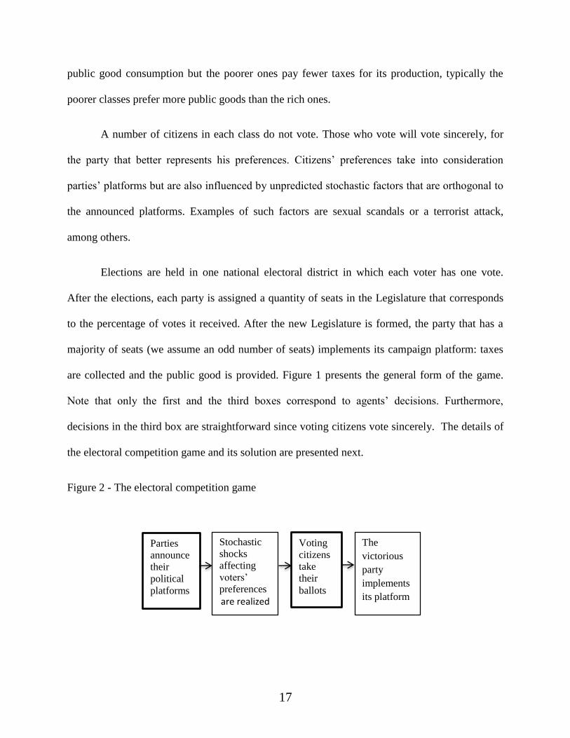
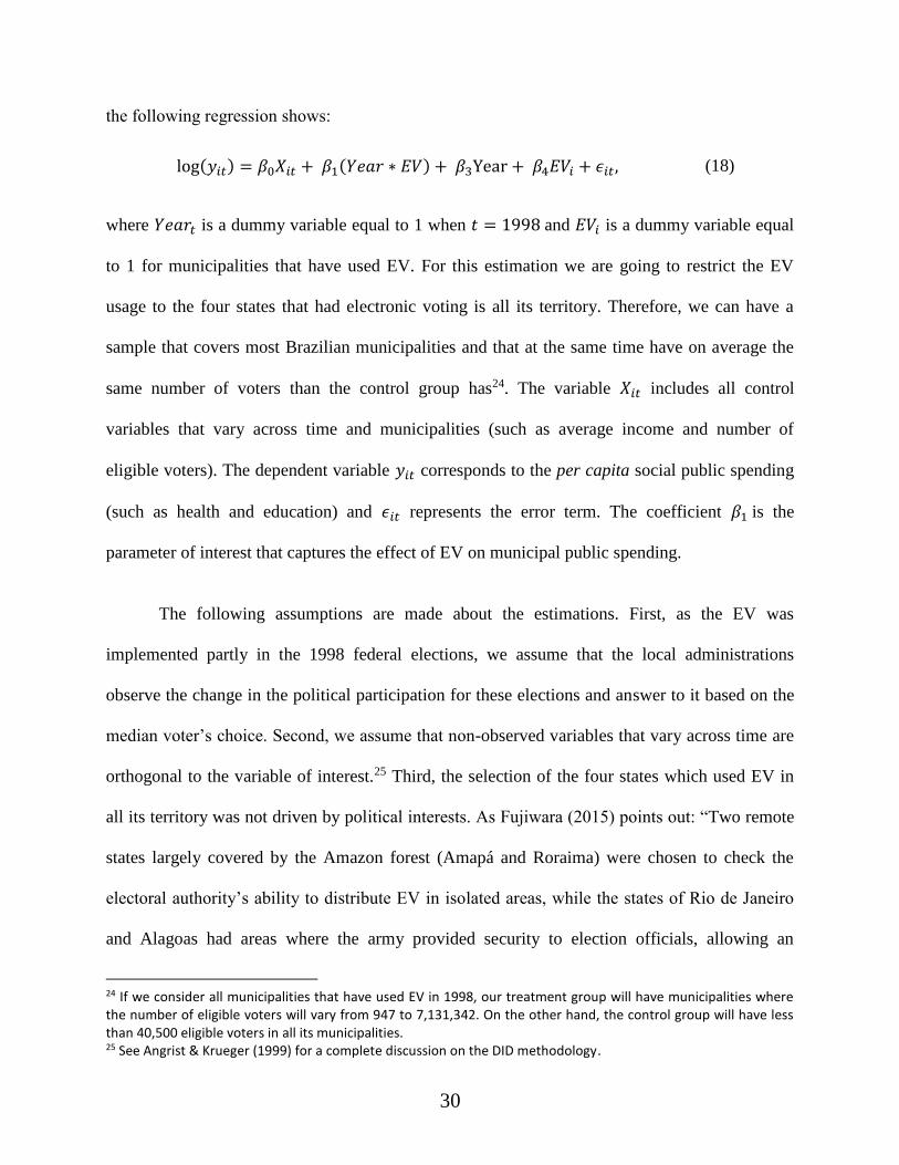
the following regression shows:

log(𝑦𝑖𝑡) = 𝛽0𝑋𝑖𝑡 + 𝛽1(𝑌𝑒𝑎𝑟 ∗ 𝐸𝑉) + 𝛽3Year + 𝛽4𝐸𝑉𝑖 + 𝜖𝑖𝑡, (18)

where 𝑌𝑒𝑎𝑟𝑡 is a dummy variable equal to 1 when 𝑡 = 1998 and 𝐸𝑉𝑖 is a dummy variable equal

to 1 for municipalities that have used EV. For this estimation we are going to restrict the EV

usage to the four states that had electronic voting is all its territory. Therefore, we can have a

sample that covers most Brazilian municipalities and that at the same time have on average the

same number of voters than the control group has24. The variable 𝑋𝑖𝑡 includes all control

variables that vary across time and municipalities (such as average income and number of

eligible voters). The dependent variable 𝑦𝑖𝑡 corresponds to the per capita social public spending

(such as health and education) and 𝜖𝑖𝑡 represents the error term. The coefficient 𝛽1 is the

parameter of interest that captures the effect of EV on municipal public spending.

The following assumptions are made about the estimations. First, as the EV was

implemented partly in the 1998 federal elections, we assume that the local administrations

observe the change in the political participation for these elections and answer to it based on the

median voter’s choice. Second, we assume that non-observed variables that vary across time are

orthogonal to the variable of interest.25 Third, the selection of the four states which used EV in

all its territory was not driven by political interests. As Fujiwara (2015) points out: “Two remote

states largely covered by the Amazon forest (Amapá and Roraima) were chosen to check the

electoral authority’s ability to distribute EV in isolated areas, while the states of Rio de Janeiro

and Alagoas had areas where the army provided security to election officials, allowing an

24 If we consider all municipalities that have used EV in 1998, our treatment group will have municipalities where the number of eligible voters will vary from 947 to 7,131,342. On the other hand, the control group will have less than 40,500 eligible voters in all its municipalities. 25 See Angrist & Krueger (1999) for a complete discussion on the DID methodology.

31

opportunity to check the logistics of distributing the electronic devices jointly with the military”.

Therefore, there seems to be no political motivation behind the EV usage selection. Fourth, the

control and treatment group do not present significant differences due to the EV usage on

variables that are not likely to be affected by it. Table 3 presents a balance check to support the

argument:

Table 3 – DID estimation showing that the treatment and control group have not changed across

periods

(1) (2) (3) (4) (5) (6) (7)

VARIABLES Valid

Votes Fed

Valid

Votes Est

Rural Income Voters HDI Illiterates

EV*Year=1998 0.22732*** 0.14187*** 0.02590 -14.80712 571.14875 0.00490 -1.71777

(0.02517) (0.02008) (0.02467) (11.91577) (369.40061) (0.00656) (1.14854)

Observations 9,760 9,760 10,222 10,222 9,761 10,222 10,222

R-squared 0.48509 0.52506 0.25971 0.61827 0.09146 0.79253 0.75642

All regressions use state fixed effects. Standard errors, clustered by mesoregion, are presented in

parenthesis. All regressions are controlled for a dummy identifying EV usage (collinear to the

state fixed effects) and a dummy identifying the year of EV usage. Regression (1), (2), (3), (4),

(5), (6) and (7) consider the valid votes to turnout ratio for federal representatives; state

representatives; percentage of people in the municipality living on rural areas; average income;

number of voters; human development index and percentage of illiterate adults. The sample

considers municipalities with more than 1245 and less than 40500 voters. *** p<0,01, ** p<0,05,

* p<0,1

Table 3 shows that the EV usage is only affecting the valid votes to turnout ratio for

federal and state representatives increasing it by 22 and 14 percentage points respectively. This

should be expected based on the previously mentioned literature on EV in Brazil. Before testing

whether the EV usage is affecting the municipal level of public spending, Figure 4 (below)

motivates the DID methodology to be applied.

32

Figure 4 – Per capita average spending on health; education; public employment, total revenue

and total spending (all values are deflated) between 1993 and 2004 comparing the municipalities

that used EV in 1998 (treatment) and the ones that didn’t (control).

The smallest 10% municipalities have been dropped to attenuate the per capita spending on the

smallest municipalities. 4577 municipalities (82% of the total Brazilian municipalities) are

covered in this representation.

As it can be observed, between 1999 and 2000 (year of the municipal election) there is a

clear increase on public spending (for all variables considered) disproportionately larger on

municipalities that used EV in 1998. It is interesting to notice that not only the electoral spending

cycle on municipal elections exist (1996, 2000 and 2004), but also that in 1996 it was

33

disproportionately larger on municipalities that didn’t use EV (public employment spending is

the only exception) making it stronger the argument that the EV has changed the municipal

social spending. In 2004, there is a clear pattern in public spending that is similar for both groups

which can be explained by the leveling on political participation in all municipalities brought by

the general usage of EV since 2000.

6.2 Results

The DID estimation results are presented in Table 4, Panel A. Columns (1), (2) and (3)

show respectively, the results obtained for social spending on health, education and public

employment. Columns (4) and (5) take into account, respectively, municipal total spending and

revenue. Finally, Column (6) shows the intergovernmental transfers, both national and

subnational (state), received by municipalities. EV usage, therefore, is responsible for an increase

in the total spending on health, education and public employment respectively by approximately

28, 20 and 22 percent.26 Total spending, revenue and intergovernmental transfers have also

increased respectively by approximately 19, 17 and 17 percent.

The intergovernmental transfer variable helps to explain how municipalities can get more

revenue in order to spend on social expenditures. As Brollo and Nannicini (2012) argue, these

transfers are extremely relevant since it accounts, on average, for 65% of the municipal budget.

However, parts of these transfers are constitutional automatic transfers such as the Fundo de

Participação dos Municípios - FPM. Therefore, it could be the case that the municipalities that

used EV in 1998 were disproportionately favored by the FPM, main source of revenue for small

26 A 28% increase on health spending, for instance, would be equivalent to an increase of 33R$ (or 16$) per capita.

34

municipalities27 and this could be driving our obtained results. The estimates presented in Table

4 control for the amount of money received by the FPM in each municipality which makes the

coefficients to get even larger showing evidence that not taking this transfer into account was

actually downward biasing the results.

Table 4 - Panel B shows the result for a similar exercise, however, instead of comparing

the public spending after the 1994 and 1998 elections, this DID analysis takes into account the

elections of 1998 and 2002 and how they do impact municipal social spending. For this counter

factual analysis one should expect the sign of the coefficient (𝛽1) to be negative since the

municipalities that didn’t use EV in 1998 are presumably going to catch up after using the new

system. Nonetheless, as EV was used by all Brazilian municipalities in 2000, one cannot isolate

its impact on public spending as clear as before. After all, one cannot argue that the 2002

elections have enfranchised voters through EV introduction. The result shows that public

spending on health was the only variable to get a negative and significant sign. The remaining

coefficients that presented significant results were positive, but their magnitudes are much

smaller than before.

Table 4 - Estimating the relationship between the logarithm of the municipal spending on public

goods (such as health and education) and the EV usage using the DID methodology.

(1) (2) (3) (4) (5) (6)

VARIABLES Health Education Public

employment

Total

spending

Total

revenue

Intergovernmental

transfers

Panel A: 1995-1996 vs. 1999-2000

Year = 1998 0.19035*** 0.25594*** 0.22464*** -0.01611 0.08540*** 0.20155***

(0.03103) (0.02713) (0.03272) (0.02367) (0.02297) (0.02049)

27 According to IBGE (the Brazilian institute of geography and statistics), municipalities with less than 5,000 citizens, between 1998 and 2000, got on average 57.3% of their revenue from FPM.

35

EV*Year=1998 0.28761*** 0.20005*** 0.22917** 0.19304*** 0.17864*** 0.17773***

(0.08616) (0.04822) (0.10282) (0.04435) (0.04063) (0.03274)

Observations 8,102 8,124 9,386 6,453 6,453 9,393

R-squared 0.38845 0.53090 0.61788 0.60570 0.63755 0.75195

Panel B: 1999-2000 vs. 2003-2004

Year = 2002 0.20743*** -0.22121*** 0.03587*** -0.43345*** -0.10971*** -0.00407

(0.01646) (0.02119) (0.01221) (0.01127) (0.01208) (0.00816)

EV*Year=2002 -0.10072** 0.07843* -0.03454 0.07165*** 0.07073*** 0.01715

(0.04181) (0.04203) (0.05620) (0.02221) (0.02673) (0.01575)

Observations 8,086 8,095 9,887 6,454 6,454 9,895

R-squared 0.40688 0.46495 0.59696 0.73215 0.67813 0.77356


parenthesis. All regressions are controlled for income, number of voters, FPM transfers and a

dummy identifying EV usage (collinear to the state fixed effects). Regression (1), (2), (3), (4),

(5), and (6) consider the logarithm of per capita municipal spending on health; education; public

employment, total spending, total revenue and total intergovernmental current transfers. The

sample considers municipalities with more than 1245 and less than 40500 voters. *** p<0,01, **

p<0,05, * p<0,1

Panel A results are close to the one presented in section 5. An interesting exercise can be

done by considering Table 3 estimations showing an increase of 14 p.p. in the valid votes to

turnout ratio for State Representatives. Plugging this value on Table 1 gives the following result:

An increase of 14 p.p. in the valid votes to turnout ratio increases health spending by 23.1%;

public employment by 10%; total spending by 13.9%; total revenue by 13.3% and

intergovernmental transfer by 20.3%. This exercise brings confidence in the results presented in

section 5 and also provides external validity to those estimations.

36

6.3 Robustness Check

The next analysis shows how intergovernmental transfers are politically motivated. This

is important to understand how municipalities that used EV can afford to spend more on social

policies. After all, even if the mayor had decided to increase social public spending he (or she)

would need to get more revenue. If the intergovernmental transfers in Brazil are politically

motivated, as argued by Brollo and Nannicini (2012), then places that have used EV should have

access to larger transfers. As argued before, the mayors act as brokers for the federal (and state)

representatives which are the ones that have access to these transfers and will benefit the mayors

that can help them to get reelected.

Table 5 shows the negative relationship between voting relatively more to the right wing

parties and social spending. The interaction variable between municipal ideology and EV usage

has a significant effect on total revenue and spending. Both get smaller once the municipality

presents larger support for the right wing parties. The variable called share shows how much of

the total vote was given to the current mayor, so this variable doesn’t change across time. As one

can notice, the interaction between this variable and EV usage is positive and significant for

education, total spending, total revenue and intergovernmental transfer. Interestingly, this

interaction squared is negative for these variables showing negative marginal returns to share of

votes. This can be an indication that places where the elections are more contested are the ones

where the mayor needs to make a larger effort to be reelected.28 Finally, a dummy indicating if

the mayor represents the same party of the governor or the president and his coalition formed

28 Federal or state representatives would be interested in helping the mayor by sending intergovernmental transfers so he (or she) can campaign for them in the federal elections two years later.

37

after the 1998 elections shows a positive and significant increase in public employment, total

spending and intergovernmental transfer only on municipalities that have used EV.

Table 5 - Estimating how the logarithm of the municipal spending on public goods (such as

health and education) and transfers are politically motivated.

(1) (2) (3) (4) (5) (6)


employment

Total

spending

Total

revenue

Intergovernmental

transfers

Year = 1998 0.19387*** 0.25756*** 0.22251*** -0.01340 0.08733*** 0.19951***

(0.03053) (0.02781) (0.03271) (0.02399) (0.02339) (0.02062)

EV*Year=1998 0.26929*** 0.17858*** 0.20476** 0.17286*** 0.16168*** 0.17162***

(0.07989) (0.04753) (0.09719) (0.03572) (0.03526) (0.03057)

Ideology -0.03823** -0.02965** -0.0610*** -0.02920** -0.02422* -0.02605**

(0.01675) (0.01449) (0.01603) (0.01368) (0.01296) (0.01053)

EV*ideol. 0.00522 -0.02738 -0.03912 -0.06711** -0.05798* -0.00762

(0.05639) (0.02677) (0.03970) (0.03341) (0.03330) (0.02115)

Share -0.00010 0.00008 -0.00008 0.00040* 0.00041* 0.00017**

(0.00017) (0.00011) (0.00015) (0.00023) (0.00023) (0.00007)

EV*Share 0.00090 0.01907*** -0.00665 0.01988** 0.02386** 0.00813*

(0.01629) (0.00683) (0.00920) (0.00999) (0.00988) (0.00429)

(EV*Share)2 0.00001 -0.0001*** 0.00006 -0.00014* -0.00017** -0.00006

(0.00016) (0.00005) (0.00007) (0.00007) (0.00007) (0.00004)

Coalition 0.00371 0.01187 0.01020 -0.00206 0.00572 0.00806

(0.01702) (0.00975) (0.01120) (0.01187) (0.01046) (0.00721)

EV*coalit. 0.14918 0.07677 0.13000*** 0.07551* 0.06412 0.05909*

(0.11098) (0.04766) (0.04833) (0.04374) (0.04229) (0.03462)

Observations 8,024 8,045 9,234 6,417 6,417 9,241

R-squared 0.39022 0.53311 0.61820 0.60674 0.63880 0.75077







p<0,05, * p<0,1

38

Next we focus on two more robustness checks: One to show that the municipal

representatives were also affected by the EV usage and another to show that the previous

findings are robust to different timing selection. The first robustness check therefore argues that

the municipal elections were also affect by the EV usage. Since there was no study showing that

the vote for municipal representatives were also impacted by the EV usage, this work used a

regression discontinuity design (RDD), as used in the previous literature (Fujiwara, 2015,

Schneider, 2015), to show that the same has happened in the municipal elections. The sample

selected takes into account the 1996 elections where State Capitals and municipalities that had

more than 200,000 voters were able to use it. Since most states, 17 out of 26, have used EV only

in one municipality and there were State Capitals with less than 200,000 voters such as Palmas-

TO with only 42,313, this work is going to select the São Paulo state to do the RDD analysis.

Almost 23% (13 out of 57) of the municipalities that used EV belonged to São Paulo state and

there were enough number of municipalities close to the cutoff to be considered29 (not the case

for the remaining states). Table 6 shows that there was an increase close to 10 percentage points

in the number of valid votes to turnout ratio for municipal representatives due to the EV usage.

Table 6 - Estimating the impact of EV usage on valid votes to turnout ratio for municipal

representatives on the municipal elections of 1996.

Valid Votes to

turnout ratio

(1)

Valid Votes to

turnout ratio

(2)

Valid Votes to

turnout ratio

(3)

VARIABLES

EV 0.08984*** 0.10077*** 0.09533***

Observations 24 22 20

29 The balance check considering number of voters and average income shows that the cutoff by itself does not bring differences between the municipalities that used EV and the remaining ones.

39

R-squared 0.64628 0.77696 0.78335

Robust standard errors presented in parenthesis. All regressions are controlled for income,

number of voters, number of voters minus the cutoff and an interaction between the former

variable and EV usage. Regression (1), (2) and (3) consider municipalities with more than

120,000; 130,000 and 140,000 voters. *** p<0,01, ** p<0,05, * p<0,1

Finally, Table 7 shows that the timing chosen for our estimations does not change the

significance or sign of our results. This table presents a DID that compares the average of

municipalities social spending between 1999 and 2000 (after federal elections) and compare it to

the average on social spending between 1997 and 1998 in order to guarantee that the mayor is

the same between these two periods. As one can notice, although the coefficients are attenuated,

they remain being positive and significant.

Table 7 - Estimating the relationship between the logarithm of the municipal spending on public

goods (such as health and education) and the EV usage using the DID methodology, but

changing the time framing.

(1) (2) (3) (4) (5) (6)


employment

Total

spending

Total

revenue

Intergovernmental

transfers

Year = 2000 0.16315*** 0.21183*** 0.12377*** 0.06551*** 0.12363*** 0.13861***

(0.01593) (0.01546) (0.01379) (0.00953) (0.01117) (0.01010)

EV* Year = 2000 0.21987** 0.11053** 0.11957** 0.13535*** 0.11783*** 0.08779***

(0.09305) (0.04605) (0.04786) (0.02382) (0.02588) (0.02842)

Observations 9,829 9,853 9,878 9,884 9,886 9,886

R-squared 0.44571 0.60489 0.66599 0.72852 0.74811 0.77797







p<0,05, * p<0,1

40

7 - Conclusion

This paper has shown that voters’ enfranchisement in Brazil, concentrated on the poor

and illiterates that were being kept from casting their votes before the electronic voting (EV)

introduction, have positively impacted the amount of social public spending on health, education

and public employment. Also, municipalities total spending and revenue as the

intergovernmental current transfers received by them, have all disproportionately increased on

municipalities using EV and therefore, presenting larger political participation. This empirical

result corroborates our model prediction that suggests larger public provision on municipalities

using EV. The main contribution of the present work is therefore to show the consequences of

EV on public spending. Finally, this work has also brought additional evidence on political

motivated intergovernmental transfer and social public spending.

References:

ALESINA, A. F.; GIULIANO, P. (2009). Preferences for Redistribution. NBER working paper

number 14825, 2009. Retrieved from: http://www.nber.org/papers/w14825.

ANGRIST, J.; KRUEGER, A. “Empirical Strategies in Labor Economics.” Cap. 23 in O.

Ashenfelter & D. Card, eds., The Handbook of Labor Economics, Volume III, North Holland,

1999.

BORGONOVI, F.; D’HOMBRES, B.; HOSKINS, B. (2010). “Voter Turnout, information

acquisition and education: Evidence from 15 European countries.” The B.E. Journal of Economic

Analysis & Policy 10(1), Article 90, 2010.

BROWN, D.; HUNTER, W. (1999). “Democracy and Social Spending in Latin America, 1980-

92.” American Political Science Review 93(4): 779-790, 1999.

BROLLO, F., & NANNICINI, T. (2012). Tying your enemy’s hands in close races: The politics

of federal transfers in Brazil. American Political Science Review, 106 (04): 742-761.

41

BUGARIN, M. and PORTUGAL, A. (2015). Should Voting Be Mandatory? The effect of

compulsory voting rules on candidates’ political platforms. Journal of Applied Economics,

18(1): 1-20.

ECONOMIST, The. “Where is it compulsory to vote?” 19 de setembro de 2013.

Disponível em: http://www.economist.com/node/21586633/

ELKINS, Z. “Quem iria votar? Conhecendo as consequências do voto obrigatório no Brasil.”

Opinião Pública 6: 109-136, 2000.

FREY, B. “Why do high income people participate more in politics?” Public Choice 11: 100-

105, 1971.

FUJIWARA, T. “Voting Technology, Political Responsiveness, and Infant Health: Evidence

from Brazil.” Econometrica 83(2): 423–464, 2015.

GREENE, K.; and NIKOLAEV, O. “Voter participation and the redistributive state.” Public

Choice 98: 213-226, 1999.

HIDALGO, D. Digital Democratization: Suffrage Expansion and the Decline of Political

Machines in Brazil. Working paper, 2010. Retrieved from: http://www.politics.as.nyu.edu/docs/

IO/17524/hidalgo.pdf.

HUSTED, T.; KENNY, L. “The effect of the expansion of the voting franchise on the size of

government.” Journal of Political Economy 105: 54-82, 1997.

IMBENS, G.; LEMIEUX, T. “Regression Discontinuity Designs: A Guide to Practice”. Journal

of Econometrics 142(2): 615-635, 2008.

JACKMAN, S. “Compulsory voting”. International encyclopedia of the social and behavioral

sciences: 16314-16318, Elsevier, 2001.

LEE, D. S.; LEMIEUX, T. Regression discontinuity designs in Economics. Journal of Economic

Literature, 48(2): 281–355, 2010.

LINDERT, P. Growing public. Social spending and economic growth since the Eighteenth

Century. Cambridge: Cambridge University Press, 2004.

MELTZER, A.; RICHARD, S. “A rational theory of the size of government.” Journal of

Political Economy 89: 914-927, 1981.

MORAES, M. F. Voting Technology and Political Competition: Lessons from Overlapping

Political Races in Brazil (master’s thesis). Universidade de São Paulo, 2012. Retrieved from:

http://www.teses.usp.br/teses/disponiveis/12/12138/tde-16042013-143746/en.php

42

MUELLER, D. & STRATMANN, T. “The Economic Effects of Democratic Participation.”

Journal of Public Economics 87(9-10): 2129-2155, 2003.

Novaes, Lucas M. 2015. “Disloyal Political Brokers and the Problem of Clientelistic Party

Building.” University of California, Berkeley. Unpublished.

PERSSON, T.; TABELLINI, G. Political economics – Explaining economic policy. Cambridge,

MA: MIT Press, 2000.

SCHNEIDER, R. (2015). Electronic Voting in Brazil: Consequences for federal representatives.

Presented at the 10th Economics Graduate Student Conference Papers. Retrieved from: http://artsci.wustl.edu/~gradconf/conf2015/Papers2015/2_2_Araujo.pdf

SCHRAM, A.; SONNEMANS, J. “Why people vote: Experimental evidence.” Journal of

Economic Psychology 17(4):417-442, 1996.

UNITED NATIONS DEVELOPMENT PROGRAM–UNDP. Democracy in Latin America:

Towards a citizen’s democracy. Buenos Aires: Aguilar, Altea, Taurus, Alfaguara, 2005.

The Economics and Politics (CNPq) Research Group started publishing its members’ working papers on June 12, 2013. Please check the list below and click at

http://econpolrg.com/working-papers/ to access all publications.

Number Date Publication

62/2016 01-13-2016 Electronic voting and Social Spending: The impact of enfranchisement on municipal public spending in Brazil, Rodrigo Schneider, Diloá Athias and Maurício Bugarin

61/2015 12-02-2015 Alunos de inclusão prejudicam seus colegas? Uma avaliação com dados em painel de alunos da rede municipal de São Paulo, Bruna Guidetti, Ana Carolina Zoghbi and Rafael Terra

60/2015 12-02-2015 Impacto de programa Mais Educação em indicadores educacionais, Luís Felipe Batista de Oliveira and Rafael Terra

59/2015 10-21-2015 Eficiência de custos operacionais das companhias de distribuição de energia elétrica (CDEEs) no Brasil: Uma aplicação (DEA & TOBIT) em dois estágios, Daniel de Pina Fernandes and Moisés de Andrade Resende Filho

58/2015 10-14-2015 Determinantes do risco de crédito rural no Brasil: uma crítica às renegociações da dívida rural, Lucas Braga de Melo and Moisés de Andrade Resende Filho

57/2015 10-07-2015 Distribuição da riqueza no Brasil: Limitações a uma estimativa precisa a partir dos dados tabulados do IRPF disponíveis, Marcelo Medeiros

56/2015 10-01-2015 A composição da desigualdade no Brasil. Conciliando o Censo 2010 e os dados do Imposto de Renda, Marcelo Medeiros, Juliana de Castro Galvão and Luísa Nazareno

55/2015 09-24-2015 A estabilidade da desigualdade no Brasil entre 2006 e 2012: resultados adicionais, Marcelo Medeiros and Pedro H. G. F. Souza

54/2015 09-24-2015 Reciclagem de plataformas de petróleo: ônus ou bônus?, Roberto N. P. di Cillo 53/2015 09-09-2015 A Progressividade do Imposto de Renda Pessoa Física no Brasil, Fábio Castro and

Mauricio S. Bugarin 52/2015 07-03-2015 Measuring Parliaments: Construction of Indicators of Legislative Oversight, Bento

Rodrigo Pereira Monteiro and Denílson Banderia Coêlho 51/2015 06-29-2015 A didactic note on the use of Benford’s Law in public works auditing, with an

application to the construction of Brazilian Amazon Arena 2014 World Cup soccer stadium, Mauricio S. Bugarin and Flavia Ceccato Rodrigues da Cunha

50/2015 04-29-2015 Accountability and yardstick competition in the public provision of education, Rafael Terra and Enlinson Mattos

49/2015 04-15-2015 Understanding Robert Lucas (1967-1981), Alexandre F. S. Andrada

48/2015 04-08-2015 Common Labor Market, Attachment and Spillovers in a Large Federation, Emilson Caputo Delfino Silva and Vander Mendes Lucas

47/2015 03-27-2015 Tópicos da Reforma Política sob a Perspectiva da Análise Econômica do Direito, Pedro Fernando Nery and Fernando B. Meneguin

46/2014 12-17-2014 The Effects of Wage and Unemployment on Crime Incentives - An Empirical Analysis of Total, Property and Violent Crimes, Paulo Augusto P. de Britto and Tatiana Alessio de Britto

45/2014 12-10-2014 Políticas Públicas de Saúde Influenciam o Eleitor?, Hellen Chrytine Zanetti Matarazzo 44/2014 12-04-2014 Regulação Ótima e a Atuação do Judiciário: Uma Aplicação de Teoria dos Jogos,

Maurício S. Bugarin and Fernando B. Meneguin 43/2014 11-12-2014 De Facto Property Rights Recognition, Labor Supply and Investment of the Poor in

Brazil, Rafael Santos Dantas and Maria Tannuri-Pianto 42/2014 11-05-2014 On the Institutional Incentives Faced by Brazilian Civil Servants, Mauricio S. Bugarin

and Fernando B. Meneguin 41/2014 10-13-2014 Uma Introdução à Teoria Econômica da Corrupção: Definição, Taxonomia e Ensaios

Selecionados, Paulo Augusto P. de Britto 40/2014 10-06-2014 Um modelo de jogo cooperativo sobre efeitos da corrupção no gasto público, Rogério

Pereira and Tatiane Almeida de Menezes 39/2014 10-02-2014 Uma análise dos efeitos da fusão ALL-Brasil Ferrovias no preço do frete ferroviário de

soja no Brasil, Bruno Ribeiro Alvarenga and Paulo Augusto P. de Britto 38/2014 08-27-2014 Comportamentos estratégicos entre municípios no Brasil, Vitor Lima Carneiro &

Vander Mendes Lucas

http://scholar.google.com/citations?user=P6YXURsAAAAJ



http://scholar.google.com/citations?user=OO5-iGcAAAAJ


37/2014 08-20-2014 Modelos Microeconômicos de Análise da Litigância, Fa ́bio Avila de Castro 36/2014 06-23-2014 Uma Investigação sobre a Focalização do Programa Bolsa Família e seus

Determinantes Imediatos. André P. Souza, Plínio P. de Oliveira, Janete Duarte, Sérgio R. Gadelha & José de Anchieta Neves

35/2014 06-22-2014 Terminais de Contêineres no Brasil: Eficiência Intertemporal. Leopoldo Kirchner and Vander Lucas

34/2014 06-06-2014 Lei 12.846/13: atrai ou afugenta investimentos? Roberto Neves Pedrosa di Cillo

33/2013 11-27-2013 Vale a pena ser um bom gestor? Comportamento Eleitoral e Reeleição no Brasil, Pedro Cavalcante

32/2013 11-13-2013 A pressa é inimiga da participação (e do controle)? Uma análise comparativa da implementação de programas estratégicos do governo federal, Roberto Rocha C. Pires and Alexandre de Avila Gomide

31/2013 10-30-2013 Crises de segurança do alimento e a demanda por carnes no Brasil, Moisés de Andrade Resende Filho, Karina Junqueira de Souza and Luís Cristóvão Ferreira Lima

30/2013 10-16-2013 Ética & Incentivos: O que diz a Teoria Econômica sobre recompensar quem denuncia a corrupção? Maurício Bugarin

29/2013 10-02-2013 Intra-Village Expansion of Welfare Programs, M. Christian Lehmann 28/2013 09-25-2013 Interações verticais e horizontais entre governos e seus efeitos sobre as decisões de

descentralização educacional no Brasil, Ana Carolina Zoghbi, Enlinson Mattos and Rafael Terra

27/2013 09-18-2013 Partidos, facções e a ocupação dos cargos de confiança no executivo federal (1999-2011), Felix Lopez, Mauricio Bugarin and Karina Bugarin

26/2013 09-11-2013 Metodologias de Análise da Concorrência no Setor Portuário, Pedro H. Albuquerque, Paulo P. de Britto, Paulo C. Coutinho, Adelaida Fonseca, Vander M. Lucas, Paulo R. Lustosa, Alexandre Y. Carvalho and André R. de Oliveira

25/2013 09-04-2013 Balancing the Power to Appoint officers, Salvador Barberà and Danilo Coelho 24/2013 08-28-2013 Modelos de Estrutura do Setor Portuário para Análise da Concorrência, Paulo C.

Coutinho, Paulo P. de Britto, Vander M. Lucas, Paulo R. Lustosa, Pedro H. Albuquerque, Alexandre Y. Carvalho, Adelaida Fonseca and André Rossi de Oliveira

23/2013 08-21-2013 Hyperopic Strict Topologies, Jaime Orillo and Rudy José Rosas Bazán 22/2013 08-14-2013 Há Incompatibilidade entre Eficiência e Legalidade? Fernando B. Meneguin and Pedro

Felipe de Oliveira Santos 21/2013 08-07-2013 A Note on Equivalent Comparisons of Information Channels, Luís Fernando Brands

Barbosa and Gil Riella 20/2013 07-31-2013 Vertical Integration on Health Care Markets: Evidence from Brazil, Tainá Leandro and

José Guilherme de Lara Resende 18/2013 07-17-2013 Algunas Nociones sobre el Sistema de Control Público en Argentina con Mención al

Caso de los Hospitales Públicos de la Provincia de Mendoza, Luis Federico Giménez 17/2013 07-10-2013 Mensuração do Risco de Crédito em Carteiras de Financiamentos Comerciais e suas

Implicações para o Spread Bancário, Paulo de Britto and Rogério Cerri 16/2013 07-03-2013 Previdências dos Trabalhadores dos Setores Público e Privado e Desigualdade no

Brasil, Pedro H. G. F. de Souza and Marcelo Medeiros 15/2013 06-26-2013 Incentivos à Corrupção e à Inação no Serviço Público: Uma análise de desenho de

mecanismos, Maurício Bugarin and Fernando Meneguin 14/2013 06-26-2013 The Decline in inequality in Brazil, 2003–2009: The Role of the State, Pedro H. G. F. de

Souza and Marcelo Medeiros 13/2013 06-26-2013 Productivity Growth and Product Choice in Fisheries: the Case of the Alaskan pollock

Fishery Revisited, Marcelo de O. Torres and Ronald G. Felthoven 12/2013 06-19-2003 The State and income inequality in Brazil, Marcelo Medeiros and Pedro H. G. F. de

Souza 11/2013 06-19-2013 Uma alternativa para o cálculo do fator X no setor de distribuição de energia elétrica no

Brasil, Paulo Cesar Coutinho and Ângelo Henrique Lopes da Silva 10/2013 06-12-2013 Mecanismos de difusão de Políticas Sociais no Brasil: uma análise do Programa Saúde

da Família, Denilson Bandeira Coêlho, Pedro Cavalcante and Mathieu Turgeon


09/2013 06-12-2103 A Brief Analysis of Aggregate Measures as an Alternative to the Median at Central Bank of Brazil’s Survey of Professional Forecasts, Fabia A. Carvalho

08/2013 06-12-2013 On the Optimality of Exclusion in Multidimensional Screening, Paulo Barelli, Suren Basov, Mauricio Bugarin and Ian King

07/2013 06-12-2013 Desenvolvimentos institucionais recentes no setor de telecomunicações no Brasil, Rodrigo A. F. de Sousa, Nathalia A. de Souza and Luis C. Kubota

06/2013 06-12-2013 Preference for Flexibility and Dynamic Consistency, Gil Riella 05/2013 06-12-2013 Partisan Voluntary Transfers in a Fiscal Federation: New evidence from Brazil, Mauricio

Bugarin and Ricardo Ubrig

04/2013 06-12-2013 How Judges Think in the Brazilian Supreme Court: Estimating Ideal Points and Identifying Dimensions, Pedro F. A. Nery Ferreira and Bernardo Mueller

03/2013 06-12-2013 Democracy, Accountability, and Poverty Alleviation in Mexico: Self-Restraining Reform and the Depoliticization of Social Spending, Yuriko Takahashi

02/2013 06-12-2013 Yardstick Competition in Education Spending: a Spatial Analysis based on Different Educational and Electoral Accountability Regimes, Rafael Terra

01/2013 06-12-2013 On the Representation of Incomplete Preferences under Uncertainty with Indecisiveness in Tastes, Gil Riella

electronic voting and social spending: the impact of

Documents