electronic coupling calculations for modelling charge
TRANSCRIPT
University College London
Department of Physics and Astronomy
Doctoral Thesis
Electronic coupling calculationsfor modelling charge transport in
organic semiconductors
Author:Fruzsina Gajdos
Supervisor:Prof. Jochen Blumberger
A thesis submitted in fulfillment of the requirements
for the degree of Doctor of Philosophy
from
University College London
September, 2016

Declaration of Authenticity
I, Fruzsina Gajdos, confirm that the work presented in this thesis is my own. Where
information has been derived from other sources, I confirm that this has been prop-
erly indicated in the thesis.


Abstract
Charge transport in organic semiconductors (OSCs) depends on a number of
molecular properties, one of which is the electronic coupling matrix element for
charge transfer between the molecules forming the material. They are the off-
diagonal elements of the electronic Hamiltonian in the charge-localised (or diabatic)
basis. The focus of this work is on the development of a method for a fast calcula-
tion of these matrix elements for OSCs. After addressing the different methods of
their calculation, I present a program to estimate the off-diagonal elements of the
Hamiltonian with a fast yet accurate semi-empirical method. This model approxi-
mates the off-diagonal elements of the Hamiltonian to be proportional to the overlap
between the orbitals of the molecules, which are projected onto a very small basis
set. The analytical results are in a reasonable agreement with accurate ab initio and
fragment orbital DFT calculations and the speed-up is up to six orders of magni-
tude compared to DFT calculations. Following on from this, the analytic overlap
method was implemented in two programs for charge carrier propagation, one based
on Kinetic Monte Carlo simulation of charge carrier hopping (presented here), the
other on surface hopping non-adiabatic molecular dynamics. I also show that the
analytic overlap method can be used to estimate non-adiabatic coupling vectors very
efficiently, which is an important quantity in surface hopping simulations.

Acknowledgments
First and foremost, I would like to thank my supervisor Prof. Jochen Blumberger
for his help and support. He provided guidance and encouragement throughout my
project, and his resilient attitude towards prioritising his students even in busy pe-
riods was invaluable during my PhD. I am also grateful to my past and present
colleagues: Dr. Adam Kubas, Dr. Marian Breuer, Jacob Spencer, Felix Hoffmann,
Dr. Po-hung Wang, Dr. Varomyalin Tipmanee, Dr. Harald Oberhofer, Guido Falk
von Rudorff, Karina Chan, Hui Yang, Dr. Ehesan Ali, Bastian Burger, Benjamin
Rousseau, Siim Valner, Felix Hummel, Jamie Sage, Marco Montefiori, Laura Scalfi,
Dr. Antoine Carof and Xiuyun Jiang for their collaboration and all the discussions
which helped in progressing this project. I would also like to thank Prof. Marcus El-
stner, Prof. Aurelien de la Lande, Dr. Natacha Gillet, Dr. Laura Berstis, Alexander
Heck and Xiaojing Wu for their collaboration. I would also like to thank Dr. Michel
Dupuis, from Pacific Northwestern National Laboratory, for his support. This work
was made possible by a joint sponsorship provided by the IMPACT studentship from
University College London and Pacific Northwestern National Laboratory.
I would like to thank the Materials Chemistry Consortium for providing access
to high performance computing facilities: HECToR and ARCHER managed by UoE
HPCx Ltd at the University of Edinburgh, Cray Inc and NAG Ltd, and funded by
the Office of Science and Technology through the High End Computing Programme
of EPSRC and the UCL Legion High Performance Computing Facility.
I would also like to thank my friends and family near and far for their love and
support. Finally, I am grateful to Dr. Ashley Shields and Thomas Beales Ferguson
who are not just brilliant friends but also helped me by commenting and proofreading
this thesis.
2

List of publications
The work discussed here has been published in the following papers:
[1] F. Gajdos, H. Oberhofer, M. Dupuis and J. Blumberger. On the inapplicability
of electron-hopping models for the organic semiconductor phenyl-C61-butyric acid
methyl ester (PCBM), Journal of Physical Chemistry Letters 4(6):1012-1017, 2013.
[2] F. Gajdos, S. Valner, F. Hoffmann, J. Spencer, M. Breuer, A. Kubas, M. Dupuis,
and J. Blumberger. Ultrafast Estimation of Electronic Couplings for Electron Trans-
fer between π-conjugated Organic Molecules, Journal of Chemical Theory and Com-
putations 10(10):4653-4660, 2014.
[3] A. Kubas, F. Gajdos, A. Heck, H. Oberhofer, M. Elstner and J. Blumberger. Elec-
tronic couplings for molecular charge transfer: benchmarking CDFT, FODFT and
FODFTB against high-level ab initio calculations. II., Physical Chemistry Chemical
Physics 17(22):14342-14354, 2015.
[4] J. Spencer, F. Gajdos, and J. Blumberger. FOB-SH: Fragment orbital-based
surface hopping for charge carrier transport in organic and biological molecules and
materials. The Journal of Chemical Physics 145(6):064102, 2016.
[5] N. Gillet, L. Berstis, X. Wu, F. Gajdos, A. Heck, A. de la Lande, J. Blumberger,
and M. Elstner. Electronic Coupling Calculations for Bridge-Mediated Charge Trans-
fer Using CDFT and Effective Hamiltonian approaches at DFT and FODFTB level.
Journal of Chemical Theory and Computations accepted, 2016.
3

Contents
1 Overview 20
2 Introduction 22
2.1 Background & motivation . . . . . . . . . . . . . . . . . . . . . . . . 22
2.2 Comparison to Si devices . . . . . . . . . . . . . . . . . . . . . . . . . 23
2.2.1 Manufacturing . . . . . . . . . . . . . . . . . . . . . . . . . . 23
2.2.2 Organic semiconducting materials . . . . . . . . . . . . . . . . 24
2.3 The structure of organic semiconductors . . . . . . . . . . . . . . . . 25
2.4 Challenges of organic semiconductors . . . . . . . . . . . . . . . . . . 28
3 Charge transport models in organic semiconductors 30
3.1 The Holstein Hamiltonian . . . . . . . . . . . . . . . . . . . . . . . . 30
3.2 Band transport . . . . . . . . . . . . . . . . . . . . . . . . . . . . . . 32
3.3 Transport via activated hopping . . . . . . . . . . . . . . . . . . . . . 34
3.4 Applicability of transport models . . . . . . . . . . . . . . . . . . . . 37
3.4.1 Non-local electron phonon coupling . . . . . . . . . . . . . . . 38
3.4.2 Mixed quantum-classical molecular dynamics . . . . . . . . . . 39
3.5 Conclusion of charge transport methods and thesis statement . . . . . 41
4 Benchmark study on the accuracy of coupling calculation methods 43
4.1 Introduction to electronic coupling calculation methods . . . . . . . . 44
4.1.1 Generalised Mulliken–Hush theory . . . . . . . . . . . . . . . 45
4.1.2 Charge Constrained DFT . . . . . . . . . . . . . . . . . . . . 47
4.1.3 Fragment orbital DFT . . . . . . . . . . . . . . . . . . . . . . 51
4

4.1.4 Density functional tight-binding . . . . . . . . . . . . . . . . . 54
4.2 Systems . . . . . . . . . . . . . . . . . . . . . . . . . . . . . . . . . . 56
4.3 Simulation details . . . . . . . . . . . . . . . . . . . . . . . . . . . . 59
4.4 Results . . . . . . . . . . . . . . . . . . . . . . . . . . . . . . . . . . . 62
4.4.1 Stacked systems . . . . . . . . . . . . . . . . . . . . . . . . . . 62
4.4.2 Randomly oriented anthracene molecules . . . . . . . . . . . . 65
4.5 Computational demands . . . . . . . . . . . . . . . . . . . . . . . . . 67
4.6 Conclusion . . . . . . . . . . . . . . . . . . . . . . . . . . . . . . . . . 68
5 Fast Analytic Overlap Method 73
5.1 Theory . . . . . . . . . . . . . . . . . . . . . . . . . . . . . . . . . . 76
5.2 Training and test sets for the parameterisation of the overlap method 80
5.3 Computational details for reference coupling calculations and fast
overlap method . . . . . . . . . . . . . . . . . . . . . . . . . . . . . . 82
5.4 Results and discussion . . . . . . . . . . . . . . . . . . . . . . . . . . 85
5.4.1 Error calculations and reference calculations . . . . . . . . . . 86
5.4.2 Overlap method with DFT orbitals . . . . . . . . . . . . . . . 87
5.4.3 Projection on the STO basis set . . . . . . . . . . . . . . . . . 88
5.4.4 Overlap method with the STO basis set . . . . . . . . . . . . 91
5.4.5 Speed-up of coupling calculations . . . . . . . . . . . . . . . . 95
5.4.6 Conclusions of the overlap method . . . . . . . . . . . . . . . 97
5.5 Analysis of heme systems with the overlap method . . . . . . . . . . 98
5.5.1 Structures . . . . . . . . . . . . . . . . . . . . . . . . . . . . . 98
5.5.2 Simulation details . . . . . . . . . . . . . . . . . . . . . . . . . 100
5.5.3 Results and discussion . . . . . . . . . . . . . . . . . . . . . . 103
5.5.4 Conclusions on the applicability of the analytic overlap method
on multi-heme systems . . . . . . . . . . . . . . . . . . . . . . 108
5
5.6 Non-adiabatic coupling vector element calculations with the fast over-
lap code . . . . . . . . . . . . . . . . . . . . . . . . . . . . . . . . . . 109
5.6.1 Assumptions of the NACV calculation with AOM . . . . . . . 110
5.6.2 Validation . . . . . . . . . . . . . . . . . . . . . . . . . . . . . 112
5.6.3 Conclusion of NACV calculation with the AOM . . . . . . . . 116
5.7 Further speed-up . . . . . . . . . . . . . . . . . . . . . . . . . . . . . 117
5.8 Conclusion . . . . . . . . . . . . . . . . . . . . . . . . . . . . . . . . . 119
6 Kinetic Monte Carlo simulations for charge carrier hopping 122
6.1 Implementation . . . . . . . . . . . . . . . . . . . . . . . . . . . . . . 123
6.1.1 Rate calculation . . . . . . . . . . . . . . . . . . . . . . . . . . 125
6.1.2 Calculating the charge carrier mobility . . . . . . . . . . . . . 129
6.2 Validation . . . . . . . . . . . . . . . . . . . . . . . . . . . . . . . . . 131
6.3 Simulation details . . . . . . . . . . . . . . . . . . . . . . . . . . . . . 135
6.3.1 Molecular dynamics trajectories . . . . . . . . . . . . . . . . . 135
6.3.2 Coupling calculation . . . . . . . . . . . . . . . . . . . . . . . 136
6.4 Results & discussion . . . . . . . . . . . . . . . . . . . . . . . . . . . 138
6.4.1 Time scales . . . . . . . . . . . . . . . . . . . . . . . . . . . . 142
6.5 Conclusion . . . . . . . . . . . . . . . . . . . . . . . . . . . . . . . . . 147
7 Conclusion & Outlook 149
7.1 Conclusion . . . . . . . . . . . . . . . . . . . . . . . . . . . . . . . . . 149
7.2 Outlook . . . . . . . . . . . . . . . . . . . . . . . . . . . . . . . . . . 152
6

List of Figures
2.1 Device setup for a pentacene–C60 heterojunction solar cell and a schematic
diagram of how the 22 pz orbitals mix into molecular orbitals creating
energetically close states around the HOMO and the LUMO creating
a band structure . . . . . . . . . . . . . . . . . . . . . . . . . . . . . 26
2.2 Crystal structure of C60 and PCBM. C60 crystallises in an FCC struc-
ture. PCBM has many different crystalline phases, here a monoclinic
phase is shown. As it can be seen, the packing is different from C60. . 27
2.3 The highest occupied molecular orbital of C−60 and PCBM−. The
orbital shapes are not very different: the side chain of the PCBM
only causes a slight perturbation in the orbital shape. . . . . . . . . . 28
7

3.1 Electronic coupling values and their effect on the energy barrier of
the localised electronic transport. The dashed line represents the
diabatic surface representing an electronic state which remains un-
changed throughout the deformation of the ionic structure. The con-
tinuous red line is the adiabatic surface representing an electronic
state which obeys strictly the Born-Oppenheimer approximation and
the electronic structure follows the ionic movements continuously and
instantaneously. The reorganisation energy is marked on the plot
with λ. Panel 1 shows the small-coupling case where the wavefunc-
tion is completely localised and transition happens on the diabatic
surface. Panel 2 shows a larger coupling where the wavefunction is
more spread out and the transition happens on the adiabatic surface.
Panel 3 shows the case when the rate equation model is beyond appli-
cability. The figures underneath illustrate schematically the density
for each state. . . . . . . . . . . . . . . . . . . . . . . . . . . . . . . . 36
4.1 This figure illustrates the steps of obtaining orbitals for FODFT wave-
function construction. The wavefunctions are minimised on the charged
isolated donor and acceptor monomers. Then, the obtained Kohn-
Sham orbitals are concatenated and orthogonalised. . . . . . . . . . . 53
4.2 The seven molecules which were stacked to assess the accuracy of
CDFT/X, FODFT, FODFTB coupling calculation methods against
GMHT+SCS-CC2 at distances ranging from 3.5 to 5.0 A. In addition,
six randomly oriented anthracene pairs were also used to assess the
effects of random orientation on the coupling values. . . . . . . . . . . 58
8

4.3 Different electronic coupling calculation method results on the stacked
systems of anthracene, tetracene, pentacene, perfluoro-anthracene,
perylene diimide, perylene and porphin compared to SCS-CC2 re-
sults depicted in a solid black line. The second panel clearly shows
the advantages of the uniform linear scaling for all methods. . . . . . 64
4.4 Randomly oriented anthracene pairs used for testing the effect of
orientation. These structures are quite different from the perfectly
stacked systems presented above. The numbers next to the panels
refer to the ID numbers presented in Table 4.4. . . . . . . . . . . . . 66
4.5 CPU time of different coupling calculation methods for different molecules
and the error bar compared to the high precision GMHT with SCS-
CC2 method. The stems refer to the mean unsigned relative error
according to Eq. (4.36); the solid stems show the scaled errors using
the scaling factors from Table 4.2 while the dashed stems show the
actual relative error of different methods. . . . . . . . . . . . . . . . . 68
5.1 This figure illustrates the steps of the projection of the SOMO onto
the pπ orbitals of the minimum Slater basis set. Panel A represents
the SOMO obtained directly from the SCF calculation. Panel B shows
the projected STO orbitals in the Cartesian coordinate system. Panel
C shows the projected rotationally invariant orbital definition, where
the orbital is expanded by the pπ orbitals (shown on a single C atom). 78
9

5.2 The arene, acene and fullerene compounds that were included in our
coupling reference calculations. The blue frame marks the training set
which was used to obtain the fitted parameters for Eq. (5.1). The red
frame marks the test set which were used independently to test the
generality of the fitted parameters. In addition, the HAB7- set shown
in Fig. 4.2 and the randomly oriented anthracene molecules were also
used as test sets. . . . . . . . . . . . . . . . . . . . . . . . . . . . . . 82
5.3 The electronic coupling decreases as a function of intermolecular dis-
tance r for three rotationally different C60 dimers. . . . . . . . . . . . 84
5.4 The correlation of the NEVPT2+GMHT coupling values with scaled
FODFT results for three different data sets: HAB7, thiophene, and
imidazole. The correlation is excellent for the stacked cases and
slightly worse for the randomly oriented thiophene molecules. . . . . . 86
5.5 The correlation of the full SCF SOMO orbital overlaps with the scaled
sFODFT coupling values. Using a different error definition to fit the
line such as MURE would have resulted in a steeper line as the higher
coupling values would have been included with a more significant weight. 89
5.6 The correlation of analytically calculated orbital overlaps using the pπ
orbitals from the minimum STO basis set with the scaled sFODFT
coupling values. . . . . . . . . . . . . . . . . . . . . . . . . . . . . . . 93
5.7 The correlation of analytically calculated orbital overlaps in the min-
imum STO basis set with the full plane wave basis set overlap values
for different molecules. . . . . . . . . . . . . . . . . . . . . . . . . . . 94
10

5.8 CPU time of different coupling calculation methods for different molecules
and the error compared to the GMHT with SCS-CC2 reference val-
ues. The colour coded stems refer to the mean unsigned relative error
Eq. (4.36); the solid stems show the scaled errors using the uniform
scaling factors from Table 4.2; while the dashed stems show the ac-
tual relative error of different methods. The analytic overlap method
is abbreviated as AOM on this plot. . . . . . . . . . . . . . . . . . . 96
5.9 Multi-heme systems extracted from MtrF (Panel A), MtrC (Panel B),
and STC (Panel C) protein SCF minimisation of the protein struc-
ture deposited in the data base. The environment of the multi-heme
structure is not visible on the panel and did not participate in the
electron structure calculations but was involved in the molecular dy-
namic simulation. The molecular dynamics calculations were done on
the entire protein structure in water. For the coupling calculations the
prophirin rings were extracted from these trajectories as in [79]. The
blue circle denotes a stacked dimer structure. The red circle shows a
T-shaped structure and the green circle is around a coplanar structure. 99
5.10 The SOMO and SOMO-1 orbitals on the perfect heme. They were
identified by the orientation of the d orbital: the SOMO and the
SOMO-1 always contain dxz and dyz where the direction z is along
the axis formed by the histidine molecules. . . . . . . . . . . . . . . . 101
5.11 On panel A, the correlation between electronic coupling and analytic
overlap values can be seen for the three different stacking types for
MtrF, MtrC , and STC. On panel B, the same correlation can be seen
for the three different multi-heme systems. The black line depicts
the best fit. The red line marks the accuracy of the cFODFT results
(0.5 meV). There is a significant variation in the coupling values even
within the different stacking types. . . . . . . . . . . . . . . . . . . . 104
11
5.12 The SOMO and SOMO-1 orbitals of a heme taken from an MD snap-
shot. Just like in the perfect heme case the orbitals were identified by
the orientation of the d orbital: the SOMO and the SOMO-1 always
contain dxz and dyz where the direction z is always along the axis
formed by the histidine molecules. However, it is worth noting that
the nodal structure on the porhyrin ring is quite different from the
one presented in Fig. 5.10 which probably has a significant effect on
the overlap. . . . . . . . . . . . . . . . . . . . . . . . . . . . . . . . . 106
5.13 On panel A, the correlation between the cFODFT coupling and the
edge-to-edge distance can be seen. On panel B, the correlation be-
tween cFODFT electronic coupling and the iron to iron distance can
be seen for the three different stacking types. . . . . . . . . . . . . . . 106
5.14 The parallelly stacked symmetric ethylene dimer system used as a test
system for NACV calculation. The intermolecular distance d was set
to 3.5 A, 4.5 A and 5.0 A. The symmetry of the dimer system was
reflected in the NACV components . . . . . . . . . . . . . . . . . . . 114
6.1 Convergence of the mobility values calculated with the finite difference
method as in Eq. (6.22) and Eq. (6.18) to the analytically obtained
mobility value as a function of the number of Monte Carlo trajectories.
The results start to converge at around 5×10⁵ trajectories. Using
more KMC trajectories changes the mobility values by less than 0.05
cm2/Vs. It can be seen here that the Einstein mobility values are
slightly overestimating the numerical and analytical derivative results
and the effect is stronger for larger couplings. . . . . . . . . . . . . . 132
12

6.2 External electric field dependency of the electron mobility with differ-
ent offsets using δE = 104 V/cm. The mobility was evaluated with the
analytic derivative method (Eq. (6.16)) and the numerical derivative
method as well (Eq. (6.22)). The E-field dependence of the mobilities
show constant mobilities at relatively low fields which starts to change
around 2× 10⁵ V/cm. The model breaks down above 106 V/cm. . . . 133
6.3 Temperature dependence of the charge mobility in a perfectly aligned
FCC C60 structure. The mobility values are calculated with three
different methods of assessing the coupling values: Einstein mobility
calculation Eq. (6.18), numerical derivative formula Eq. (6.22), and
the analytical mobility Eq. (6.16). . . . . . . . . . . . . . . . . . . . . 134
6.4 The two bond types present in C60. Although both bonds are between
sp2 carbons they differ in length and binding energy. . . . . . . . . . 137
6.5 Distribution of the electronic coupling values for FCC C60 crystal at
300 K for a 1 ns trajectory. The neighbour distance cut-off was 15 A
including nearest and second nearest neighbours. The RMS averaging
of the coupling values according to Eq. (6.23) resulted in relatively
narrow peaks. . . . . . . . . . . . . . . . . . . . . . . . . . . . . . . . 139
6.6 Distribution of the electronic coupling values for FCC C60 crystal at
different temperatures for a 1 ns trajectory along the three axes for the
nearest neighbours only. The 300 K trajectory on Panel A shows an
isotropic distribution of coupling values while the 100 K trajectory has
distinct peaks and in the z direction the distribution differs from the
almost identical x and y directions. This is due to the phase transition
in the crystalline C60 below 100K which prevents free rotation of the
molecules. Such coupling distribution indicates that while at 300 K
the mobility tensor is expected to be isotropic at 100 K this may not
be true. . . . . . . . . . . . . . . . . . . . . . . . . . . . . . . . . . . 140
13
6.7 Distribution of the Hij values in FCC C60 crystal at 300 K for a 100 ps
trajectory when no RMS averaging is applied to the coupling values.
The mean is 13 meV while the maximum coupling is 73 meV. . . . . 141
6.8 Distribution of the site energy difference for FCC C60 crystal at 300
K for a 100 ps trajectory. The energy peaks form a Gaussian with a
mean of 0 meV and a standard deviation of 52.3 meV. . . . . . . . . 141
6.9 Discrete cosine transform of the electronic coupling for a dimer in
a FCC C60 crystal at 300 K for a 100 ps trajectory. The spectrum
is dominated by slowly changing parameters. This corresponds to
our expectations that in the case of C60 the rotation has the most
significant effect on the coupling. . . . . . . . . . . . . . . . . . . . . 143
6.10 Discrete cosine transform of the site energy difference for a dimer in
a FCC C60 crystal at 300 K for a 100 ps trajectory. The lower peak
at 487 cm−1 corresponds to the breathing mode of the C60 cage. The
higher frequency term is comparable to the frequency of a carbon
double bond stretch. . . . . . . . . . . . . . . . . . . . . . . . . . . . 143
6.11 The probability distribution of the hopping rate with three different
types of parameter averaging. As it can be seen the instantaneous site
energy difference has a strong effect on the rate distribution, while the
averaged Hab values create a sharp rate distribution. . . . . . . . . . . 145
6.12 The probability distribution of the hopping rate compared to the
Fourier transform of the site energy difference and the Fourier trans-
form of the electronic coupling values. It can be seen that rates are
in general slower than the site energy difference changes, while the
difference is not so straightforward for the coupling timescales. . . . . 146
14
List of Tables
4.1 Electronic coupling matrix element values for the negatively charged
symmetric perfectly stacked dimers of anthracene, tetracene, pen-
tacene, perfluoro-anthracene, perylene-diimide, perylene and porphin
at d separation calculated with SCS-CC2+GMHT, CDFT/X, FODFT,
and FODFTB methods for the HAB7- set, where X denotes the per-
centage of Hartree–Fock exchange. All coupling values are in meV.
The error values for each method were calculated according to Eqs.
(4.36) using SCS-CC2+GMHT results as reference values. . . . . . . 71
4.2 Revisited Hab errors after uniform linear scaling is applied to all ap-
proximate coupling values compared to SCS-CC2 reference values for
the stacked systems. The prefix ‘s’ refers to the scaled values. . . . . 72
4.3 Distance dependence of the coupling values according to Eq. (4.37)
with the different coupling calculation methods. All β values are in
A−1
. The error values with respect to SCS-CC2+GMHT reference
values were calculated with Eqs. (4.36). . . . . . . . . . . . . . . . . . 72
4.4 Coupling results for the randomly oriented anthracene dimers. d
marks the closest C-C distance between the dimers. All coupling
values are in meV. The mean unsigned error is calculated according
to Eq. (4.36) using the SCS-CC2 coupling values as reference. . . . . 72
5.1 Analysis of the exponential decay constant of the overlap according
to Eq. (4.37) and the R2 value of the fitted lines. . . . . . . . . . . . 84
15

5.2 Correlation of the GMHT+NEVPT2 and sFODFT coupling values
for HAB7, thiophene, and imidazole. MRUE, MUE, and MAXERR
values were calculated according to Eq. (4.36). . . . . . . . . . . . . . 87
5.3 Errors of the calculated Hab values using Eq. (5.1) with full SCF basis
set compared to the sFODFT Hab values. ERMSLE values give a
rough estimate of the factor of the error therefore there are no units
presented. . . . . . . . . . . . . . . . . . . . . . . . . . . . . . . . . . 88
5.4 Different µC2p values for the projection give different completeness (See
Eq. (5.9)). The completeness of the monomers of the HAB7 set were
averaged. The HAB7 set was not very sensitive tox changes in the
Slater coefficient, but the C60 set had stronger µ dependency. . . . . 89
5.5 Orbital norms calculated with the analytic overlap program using SCF
orbitals projected on the minimum STO basis set. The calculations
marked with s included the s orbitals too while the unmarked overlap
values only contain the pπ orbitals orthogonal to the plane of conju-
gation. 〈||φ′ND ||〉 refers to the mean of the norm while σ(||φ′ND ||
)is
the standard deviation. The molecules of the HAB7 and acenes data
set were unaffected by the inclusion as the s coefficients were 0. . . . 91
5.6 Different µC2p values around the best fitted µC
2p and the conversion fac-
tor C which approximates best the sFODFT coupling values according
to Eq. (5.18). Relative and logarithmic errors calculated according to
Eq. (4.36) and Eq. (5.13) respectively. . . . . . . . . . . . . . . . . . . 92
5.7 Different µC2s values and the corresponding ERMSLE values on the
training set comparing approximate coupling values calculated with
Eq. (5.18) to sFODFT reference values. The effect of the s orbitals is
much smaller compared to the p orbitals. The value of the conversion
factor was not affected by the larger basis set. All values are in bohr−1. 92
16
5.8 The errors of the analytically calculated Hab values compared to the
sFODFT Hab values. ERMSLE and MAXUL values give a rough
estimate of the factor of the error therefore these values are unitless
and were calculated according to Eq. (5.13) and Eq. (5.14). . . . . . . 93
5.9 Overlap values in the full SCF plane wave and the reduced minimum
STO basis set for PCBM with and without including the phenyl group
for different configurations, denoted as Sab, Sab and S ′ab respectively.
It can be seen that for the configuration with no stacking the effect
is negligible but for those where there is phenyl stacking the effect is
significant. . . . . . . . . . . . . . . . . . . . . . . . . . . . . . . . . . 95
5.10 Average Fe-to-Fe and edge-to-edge distance of the different types of
heme dimers. The edge-to-edge distance was calculated using the
smallest distance between the carbon atoms of the porphyrin rings.
The numbers in the brackets show the maximum deviation from the
average values for each stacking type. . . . . . . . . . . . . . . . . . . 100
5.11 cFODFT coupling values as a function of the plane wave basis set for
assessing an optimal and sufficient basis set. Both couplings are from
MtrC. Structure A is a coplanar dimer and structure B is a stacked
dimer. . . . . . . . . . . . . . . . . . . . . . . . . . . . . . . . . . . . 101
5.12 Proportionality constants for different cFODFT coupling and AOM
overlap correlations for the different stacking types on their own and
combined with other stacking types. . . . . . . . . . . . . . . . . . . . 104
5.13 Proportionality constants for different cFODFT coupling and AOM
overlap correlations including MtrF, MtrC, and STC in one fit. For
some of the fits certain values were omitted based on the stacking type.105
17

5.14 Exponential decay as a function of edge-to-edge distance for cFODFT
coupling values. To reduce errors the coupling values were binned
together. The bins were 0.5 A wide. The fit was made to different
selections: stacked stands for stacked only, stacked+T is fitted to the
joint group of stacked+T-shaped; and all includes every stack type,
stacked, T-shaped, and coplanar. . . . . . . . . . . . . . . . . . . . . 107
5.15 Exponential decay as a function of Fe-Fe distance for cFODFT cou-
plings. To reduce errors the coupling values were binned together.
The bins were 0.5 A wide. The fit was done including all stacking
types for all three proteins. . . . . . . . . . . . . . . . . . . . . . . . . 108
5.16 NACV component calculation robustness with FODFT and analytic
overlap method as a function of different δR values for the finite dif-
ference method as in Eq. (5.22). . . . . . . . . . . . . . . . . . . . . . 113
5.17 NACV calculations with three different methods at different dimer
separations on a perfectly stacked ethylene dimer. In the case of
the reference FODFT method, the wavefunction is relaxed on the
distorted structure and the overlap is calculated between the full or-
bitals. The hybrid method relaxes wavefunctions which are projected
onto the minimum STO basis set and calculates the overlap analyti-
cally. The AOM uses the undistorted STO coefficients and calculates
the overlap analytically. The results are calculated at different dis-
tances. The letters refer to the type of atom and the direction of the
NACV element. . . . . . . . . . . . . . . . . . . . . . . . . . . . . . . 116
5.18 Different atomic overlap cut-offs, and their effect on the overlap cal-
culation accuracy and computational time demonstrated on two C60
dimers one with a large overlap value, and another one with a small
one. . . . . . . . . . . . . . . . . . . . . . . . . . . . . . . . . . . . . 119
18
6.1 Configurational change in the isolated C60 due to excess charge ex-
pressed in the change of the bond length of the two bond types present
in C60. RC denotes the geometry optimised with an excess charge;
RN is the neutral optimised nuclear configuration. The overall effect
is a slightly elongated buckyball in one direction. . . . . . . . . . . . 137
6.2 Mobility values calculated with the different methods at different tem-
peratures. µana is calculated with the analytic evaluation method Eq.
(6.16), µE is calculated with the Einstein relation Eq. (6.18), and µnd
is calculated with the numerical derivative formula Eq. (6.22). At 300
K and 500 K the material was isotropic: all three mobility values were
the same. All mobility values are in cm2/Vs. . . . . . . . . . . . . . . 147
6.3 Mobility values calculated with the different methods at 100 K. µE is
calculated with the Einstein relation Eq. (6.18), and µnd is calculated
with the numerical derivative formula Eq. (6.22). All mobility values
are in cm2/Vs. . . . . . . . . . . . . . . . . . . . . . . . . . . . . . . . 147
19

1 Overview
Due to their numerous favourable characteristics - for example their light weight and
low fabrication costs - organic semiconductors (OSCs) are becoming an increasingly
prominent part of the semiconductor industry. However, low efficiency, which partly
arises from low charge mobility, means that organic devices cannot compete with
their inorganic counterparts. One of the key issues in current OSC devices is that
little is known about their actual charge transfer mechanism. Commonly applied
theoretical methods often assume either completely delocalised band-like transport
or completely localised electron hopping transport. However, both experimental and
theoretical results show that neither of the models above are applicable in many
cases. Furthermore, both models underestimate the role of thermal fluctuations
which create dynamic disorder in these materials. Although several generic quan-
tum models have been suggested to tackle this issue, most of them can only be solved
for small systems which cannot represent disordered media. Non-adiabatic molecular
dynamics provides a possible solution which omits any assumptions with respect to
localisation. In order to be able to apply it in large systems, the efficient calculation
of the electronic Hamiltonian matrix elements and the non-adiabatic coupling vec-
tors is crucial.
The aim of this work is to discuss charge transport in organic semiconductors
and to provide the tools to enable fast and accurate charge transport modelling. In
Chapter 2, a brief summary of the role of organic semiconductors (OSCs) in indus-
try is followed by a description of the defining characteristics and structure of OSCs.
This thesis describes the limitations of different theoretical transport models with an
20

emphasis on the most common current techniques and analysing their applicability
in Chapter 3. Firstly, the two most popular transport models in organic semicon-
ductors, band transport and hopping, are presented. As neither of these models
describes charge transport in organic semiconductors generally and satisfactorily, a
possible alternative, the mixed quantum-classical molecular dynamics model, is pre-
sented. While mixed quantum classical molecular dynamics is a versatile tool, it is
also pointed out that it is computationally intensive. In particular, it requires the
fast and accurate calculation of electronic Hamiltonian coupling matrix elements,
the overlap matrix, and non-adiabatic coupling vectors. The importance of calcu-
lating accurate electronic Hamiltonian off-diagonals is underlined. In Chapter 4, a
detailed analysis of different coupling calculation methods is discussed for a wide
range of organic molecules in the reduced state. To this end, a selection of cou-
pling calculation methods of different quantum levels are compared and analysed
with respect to accuracy and computational demands on a broad range of organic
molecules. Finding a less computationally intensive alternative to the presented
methods led to the development of a fast yet accurate method for the calculation of
off-diagonal Hamiltonian elements. Chapter 5 presents the analytic overlap method
and discusses theory and application, accuracy, and statistics on the computational
demand which enable the application of otherwise costly mixed quantum-classical
molecular dynamics on systems large enough to capture the behaviour of realistic
organic semiconductors. The method is also implemented into a Monte Carlo code,
which assumes hopping of localised charge carriers. Details of these calculations are
presented in Chapter 6. After concluding this work in Chapter 7, further avenues of
investigation are also outlined.
21

2 Introduction
The following chapter provides a basic introduction to the increasing prevalence of
organic semiconductors in the semiconductor industry and outlines the most funda-
mental differences between organic and inorganic semiconducting devices. Following
this, a brief summary of the most common semiconducting devices is presented along
with a few recent results on promising new materials. The chapter is concluded with
discussing the structure of organic semiconductors and the issues arising from it with
regard to the analysis of charge transport in these materials.
2.1 Background & motivation
There is a clear demand for ever lighter and cheaper electronic devices. According to
the Business Insider, between 2007 and 2015 the number of smartphones sold grew
from 120 million to 1.4 billion units, the lifespan of an average phone is less than 5
years and 99% of the disposed mobile phones end up in landfill. Adjusting to con-
sumer preferences, manufacturers are decreasing the thickness of these devices which
brings new materials into scope. Organic semiconductors offer a cheaper and more
versatile alternative to inorganic counterparts. They are made from fairly inexpen-
sive materials, their production demands fewer resources than silicon counterparts,
their fabrication process is simpler and linear and a high proportion of the devices
are biodegradable [1].
The theoretical limit of electron mobility in organic semiconductors is less than
the the typical mobilities of 1000 cm2/Vs in pure silicon single crystals, therefore it is
unlikely they will replace devices where such high mobility and a highly ordered envi-
22

ronment are essential. However, in recent years high mobility organic semiconductors
were shown to have mobilities which are comparable to electronics grade amorphous
and polycrystalline silicon (a-Si and poly-Si with typical mobilities of≈1 cm2/Vs
and ≈100 cm2/Vs respectively). Therefore currently, organic semiconductors are
regarded as an alternative to a-Si and poly-Si devices: organic field effect transistors
(OFETs) which can be used in organic light emitting displays [2] and radio frequency
identification (RFID) tags [3], organic light-emitting diodes (OLED)[4], and organic
photovoltaic devices (OPV) [5]. OLED displays are currently used by many com-
panies in wearable devices as they are thinner and lighter than inorganic devices.
Furthermore, the active matrix display does not require background lighting as the
thin film is light emitting on its own which creates a preferable black contrast and
makes them more energy efficient on mostly black screenshots despite lower overall
efficiency. Similarly, OFETs are also used to make large curved displays. Although
organic photovoltaics are less efficient than their silicon counterparts (mobilities of
≈0.1-1 cm2/Vs), their cheap fabrication facilitates large area production. In addi-
tion, the low cost of manufacturing also means a lower energy payback time, which
makes OPVs an appealing area for research. Even though nowadays the focus has
shifted towards perovskite photovoltaics, another promising cheap and efficient al-
ternative to amorphous and polycrystalline Si devices, OPVs can compete in large
area applications as they do not contain heavy metals such as Pb making them a
safer option.
2.2 Comparison to Si devices
2.2.1 Manufacturing
While Si processing requires high temperatures and vacuum even with highly ef-
ficient plasma enhanced chemical vapour deposition, around 150-500 C [6], single
23

crystal organic semiconductors can be fabricated at temperatures as low as 90 C
[5]. Ambient temperatures can also be used when the OSCs are produced with drop
casting [7], dip casting [8] and spin casting [9]. Furthermore, devices can be pro-
duced from solution using specialised ink jet printers [10]. A great added advantage
of the ambient processing temperature is that it allows OSC devices to be processed
on flexible substrates [11, 12].
2.2.2 Organic semiconducting materials
The variety of available materials which can be used as organic semiconductors
presents a wide range of charge mobility and band gap values. While inorganic n-
type and p-type semiconductors are usually created by doping, in the organic case
it is often the material itself which has a large electron affinity or a low ionisation
potential [13].
p-type organic semiconductors
A wide variety of p-type materials are available including small molecule single crys-
tals consisting of acenes or rubrene and polymers like poly(2,5-bis(3-hexadecylthiophen-
2-yl)thieno[3,2-b]thiophene (PBTTT), poly(3-hexylthiophene-2,5-diyl (P3HT), and
diketopyrrolopyrrole (DPP), all three of which are commonly used in bulk hetero-
junction photovoltaics [14, 15, 16]. In some materials rather high mobilities were
measured: in air stable rubrene single crystals mobilities exceeding 10 cm2/Vs were
measured [17], while mobilities exceeded 40 cm2/Vs for highly aligned meta-stable
structure of 2,7-dioctyl[1]benzothieno[3,2-b][1]benzothiophene (C8-BTBT) accord-
ing to Ref [13]. Polymers mostly have lower mobilities of around a few cm2/Vs due
to their partial disorder, however there is evidence for mobility values as high as
10.5 cm2/Vs in highly ordered DPP [16].
24

n-type organic semiconductors
There are far fewer known n-type organic semiconductors than p-types and many
n-type OSCs are ambipolar carrying electrons and holes equally well which leads
to inefficient power usage. The mobility in n-type semiconductors is also generally
lower. Nevertheless, there is an increasing demand for n-type and ambipolar organic
semiconductors for OPVs. One way of creating n-type semiconductors is introducing
electron withdrawing groups to otherwise p-type semiconductors like in the case of
perylene-diimide, naphthalene-diimide and fluorinated rubrene. The typical electron
mobility for these materials ranges between 1 to 4 cm2/Vs, an order of magnitude
smaller than what is achievable in p-type organic semiconductors [18]. The best
performance so far has been achieved in C60 single crystal needles where mobilities
as high as 11 cm2/Vs were measured [13].
2.3 The structure of organic semiconductors
The principle behind the application of π-conjugated molecular systems as semi-
conductors is that the p orbitals of sp2 hybridised carbon atoms form delocalised,
energetically closely spaced states where the energy difference between the highest
occupied level and the lowest unoccupied level is similar but slightly larger than that
of inorganic semiconductor crystals [9]. Despite their higher band gap these materi-
als behave like semiconductors when charge carriers are injected through electrodes.
Although this similarity inspired the first successful experiments on OSC devices,
the charge transport processes in these devices seem to be fundamentally different
from those in inorganic systems.
The microstructure of small molecule organic semiconductors depends on the
fabrication process and the materials used, and it ranges from amorphous to poly-
and semicrystalline to single crystalline [19, 20, 21, 22]. However, all organic semi-
conducting materials share the common feature of being held together by weak van
25
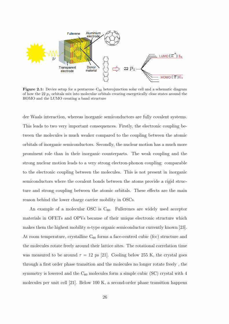
Figure 2.1: Device setup for a pentacene–C60 heterojunction solar cell and a schematic diagramof how the 22 pz orbitals mix into molecular orbitals creating energetically close states around theHOMO and the LUMO creating a band structure
der Waals interaction, whereas inorganic semiconductors are fully covalent systems.
This leads to two very important consequences. Firstly, the electronic coupling be-
tween the molecules is much weaker compared to the coupling between the atomic
orbitals of inorganic semiconductors. Secondly, the nuclear motion has a much more
prominent role than in their inorganic counterparts. The weak coupling and the
strong nuclear motion leads to a very strong electron-phonon coupling: comparable
to the electronic coupling between the molecules. This is not present in inorganic
semiconductors where the covalent bonds between the atoms provide a rigid struc-
ture and strong coupling between the atomic orbitals. These effects are the main
reason behind the lower charge carrier mobility in OSCs.
An example of a molecular OSC is C60. Fullerenes are widely used acceptor
materials in OFETs and OPVs because of their unique electronic structure which
makes them the highest mobility n-type organic semiconductor currently known [23].
At room temperature, crystalline C60 forms a face-centred cubic (fcc) structure and
the molecules rotate freely around their lattice sites. The rotational correlation time
was measured to be around τ = 12 ps [21]. Cooling below 255 K, the crystal goes
through a first order phase transition and the molecules no longer rotate freely , the
symmetry is lowered and the C60 molecules form a simple cubic (SC) crystal with 4
molecules per unit cell [21]. Below 100 K, a second-order phase transition happens
26

and the rotation stops [24].
Figure 2.2: Crystal structure of C60 and PCBM. C60 crystallises in an FCC structure. PCBMhas many different crystalline phases, here a monoclinic phase is shown. As it can be seen, thepacking is different from C60.
Although C60 has many favourable characteristics [23], there are limited ways of
processing them and for this reason they are often functionalised by adding polar
groups. For example, phenyl-C61 butyric acid methyl ester (PCBM) is a derivative
of C60 with an added polar side chain (Fig 2.3). This makes the fullerenes soluble in
chlorobenzene and dichlorobenzene which facilitates their solvent casting [5, 7]. Al-
though these functional groups do not affect the electronic structure of the molecules
dramatically, as can be seen in Fig. 2.3, they lead to a significant change in the crys-
tal packing (Fig. 2.2). For example, PCBM is known to form triclinic [5], monoclinic
[5, 7] and hexagonal [25] structures. Although currently there is no known experi-
mental data on mobility in single crystal PCBM it is expected to be similar to that
of C60 but that is dependent on the stacking in the given crystal structure.
It is also interesting to consider how the side chains change the dynamics in
the crystal and affect the dynamic disorder. As free rotations of the C60 cages are
prevented by the polar groups, this is expected to change the nature of the thermal
fluctuations and to have an effect on the charge transport [7].
Due to their numerous interesting characteristics and popularity, fullerenes will
play an important role in this piece of work.
27

Figure 2.3: The highest occupied molecular orbital of C−60 and PCBM−. The orbital shapes arenot very different: the side chain of the PCBM only causes a slight perturbation in the orbitalshape.
2.4 Challenges of organic semiconductors
As mentioned, despite their positive characteristics, organic compounds cannot com-
pletely overtake the semiconductor market due to their significantly lower efficiency
in which low electron mobility is a major factor [26]. Whilst the charge mobility in
inorganic semiconductors is in the order of 1000 cm2/Vs, the upper limit in organic
molecular crystals is two orders of magnitude smaller even in highly purified single
crystalline samples. In fact, even the basic question of whether the charge carriers ex-
hibit a wavelike behaviour, delocalised over the sample, or whether they are localised
on one (or a few) molecules and maintain their particle behaviour during the trans-
port, remains unanswered. The particle/wave like behaviour of the excess charge
affects the charge recombination mechanisms in these materials which is one of the
main sources of lower efficiency in organic semiconducting devices. Experimental
evidence seems to support both theories. In high purity samples experimental re-
sults show that at low temperatures the electron mobility decreases with increasing
temperature which suggests non-thermally-activated charge transport. The Hall-
effect [20, 27] has also been measured in organic crystals. These both suggest wave
28
like behaviour. On the other hand, electron spin resonance (ESR) results show lo-
calised charge carriers in similar samples [28]. These controversial results call into
question the applicability of models that make assumptions on the localisation or
delocalisation of the charge carrier.
In order to improve the efficiency of OSCs, it is crucial to have a general under-
standing of charge transport which is applicable to a wide range of materials, regard-
less of whether the system is crystalline, polycrystalline or amorphous [26, 29, 30, 31].
Such a model should be able to account for both the static and dynamic disorder
introduced by the relatively weak interaction and should also be feasible in large
system sizes in order to get a better description of realistic OSC materials.
29

3 Charge transport models in or-
ganic semiconductors
In the previous chapter, it was briefly mentioned that the major challenges of simulat-
ing electron transport in organic semiconductors arise from the many non-negligible
energy terms which have to be included in the Hamiltonian. Furthermore, accu-
rate modelling requires large system sizes in order to fully understand the structural
characteristics. In this chapter, several approximations are presented for assessing
the charge transport in organic semiconductors. First, a model Hamiltonian is in-
troduced for organic semiconductors. Then, the two most common charge transport
approximation methods are discussed: band transport, and small polaron hopping.
Finally, other more general but computationally intensive methods such as non-
local electron-phonon coupling and non-adiabatic molecular dynamics are presented,
which can offer a method for tackling the issues of charge transport in organic semi-
conductors where the two previous methods fail.
3.1 The Holstein Hamiltonian
A commonly used model Hamiltonian is the Holstein Hamiltonian [32]. It describes
the polaron—the combination of an excess charge and the associated deformation—
and is used by Troisi [33], Bredas [34], and Sirringhaus [35]. It can be written in the
following form
H = Hel−el +Hnuc−nuc +Hel−nuc. (3.1)
30

The operator H consists of an electronic part Hel−el, a nuclear part Hnuc−nuc, and the
term that expresses the relationship between them, including the electron phonon
coupling Hel−nuc. The weak intermolecular interaction between the molecules means
that the couplings (0.1 to 100 meV) are most of the time an order of magnitude
smaller than the energy gap between the orbitals (1 eV). As a consequence, the
orbitals of the individual molecules are only slightly perturbed in the condensed
phase. This means that the wavefunction of a charge carrier can be well represented
by linear combinations of the orbitals of the isolated diabatic states. Consequently,
the electronic part of the Hamiltonian can be approximated by localised diabatic
states on site i, denoted as |i〉. Therefore, the electronic Hamiltonian may be written
in the form of
Hel−el =∑i
Hi|i〉〈i|+∑j
Hij|i〉〈j| (3.2)
where Hi is the on-site energy, and Hij is the electronic coupling between the states
localised on the different sites. Now, as mentioned before, the coupling between
the sites is rather weak and even the second nearest neighbour term is often orders
of magnitude smaller than the nearest neighbour contribution. Thus, usually only
the nearest neighbour terms are kept. It is also worth mentioning that the large
difference between the orbital energy gap and the coupling is often used as a reason
to use approximate fragment orbital methods so that the diabatic state is replaced by
highest occupied molecular orbitals (HOMOs) of the molecules (which are also called
as singly occupied molecular orbitals, or SOMOs, in case of open-shell systems). The
nuclear motion is approximated as a sum of harmonic oscillators:
Hnuc−nuc =∑k,i
~Ωk,i
2(a+
k,iak,i +1
2), (3.3)
where a+k,i and ak,i are the creation and annihilation operators of the phonon de-
scribed by the angular frequency Ωk,i and k is the wave vector. The expression for
Hnuc−nuc can be simplified like in the case of the works by Coropceanu et al. [36]
31

where only the dominant normal mode is chosen. In this case, the nuclear motion is
to be described with a single classical harmonic oscillator
Hnuc−nuc =∑i
~Ω
2(p2i + q2
i ), (3.4)
where qi is the nuclear deformation along the chosen phonon mode, pi is the associ-
ated canonical momentum and Ω is the frequency of the dominant optical phonon.
The third term is the electron-phonon coupling value. In this semi-classical interpre-
tation the electron phonon coupling is expected to be weak and thus only the linear
component is kept. The expression is as below
Hel−nuc = g~Ωqi|i〉〈i| (3.5)
where g is the coupling strength of the local electron-phonon coupling [37].
3.2 Band transport
In the low-temperature limit (hΩ >> kBT ), the nuclear motion is negligible and the
charge carrier and associated deformation remain delocalised forming the polaronic
band [32]. Assuming that the electron phonon coupling is negligible, this expression
can be simplified by thermally averaging over the different Hij values in the form of
Hband =∑i
H ′i|i〉〈i|+H ′ij|i〉〈j|, (3.6)
where H ′ij = Hij exp(−1
2g2(NΩ + 1
2
))and the term NΩ has a non-trivial tempera-
ture dependence
NΩ =
(exp
(~Ω
kBT
)− 1
)−1
(3.7)
increasing as the temperature increases [32]. For this Hamiltonian, the Boltzmann
equation can be used to acquire mobility values [22].
32

The mobility can be calculated as
µ =−etsm∗
(3.8)
where the relaxation time between collisions ts can be calculated from the auto-
correlation function of the velocity of the electrons obtained from the first velocity
moment of the distribution function [38].
〈v(0)v(t)〉 = 〈v2〉 exp
(− t
ts
)(3.9)
The effective mass tensor can be calculated as
m∗−1lm =
1
~2
∂2E
∂kl∂km(3.10)
where kl and km are reciprocal space vector components and E is the full energy
expression according to Eq. (3.6). Using the example of a homogeneous one-
dimensional chain by Troisi [26], the effective mass tensor simplifies to the following
scalar:
m∗ =~2
2a2|Hij|(3.11)
where a is the lattice constant in the one dimensional chain. As expected, the higher
the coupling, the lower the effective mass. Strong couplings imply nearly deloclised
states with large mobilities and therefore small effective mass values. One can see
that in Eq. (3.6), H ′ij < Hij for T > 0 K, therefore the effective mass increases as the
temperature increases causing the mobilities calculated with the Boltzmann-equation
to decrease.
As predicted above, high mobility values were observed in highly purified naph-
thalene and perylene samples [39] and Hall-effect was measured in rubrene [27].
Furthermore, in the low temperature limit the temperature dependence becomes
33

µ ∝ T−n, similar to inorganic semiconductors. However, as the temperature in-
creases the nuclear motion becomes more significant and band theory breaks down
as the electron-phonon coupling becomes more relevant. Indeed localisation has
been observed in ESR [28] and CMS [40] spectroscopy. This observed localisation
prompted the idea of using other transport models, such as activated hopping.
3.3 Transport via activated hopping
In the limit of high-temperature and small electronic coupling, the charge carrier
and the associated deformation become localised on one molecule and form a small
polaron which remains localised during the transport. This limit can be treated
with localised charge hopping theory which has been used to assess the rate of
oxidation and reduction in solutions [41]. In this case, the electron is localised on
one site. In order to move, the electron has to overcome an energy barrier which
is an infrequent Markovian process and can be treated using transition state theory
with semi-classical reaction rates [42, 43]. The localised transport can be explained
by showing the potential energy surfaces of the transport presented in Fig. 3.1.
When Hab is small compared to the reorganisation energy λ of the molecules and
the surroundings, the transition occurs on the diabatic surface (Panel 1 Fig. 3.1).
This falls under the Marcus theory which has been used to describe charge transport
in solutions [42]. The rate of the transition is given by
kna =2π
~|Hab|2
1√4πλkBT
exp
(−(∆A+ λ)2
4λkBT
)(3.12)
where ∆A = Aa − Ab is the potential energy difference between the two energy
minima on the diabatic surfaces. For large electron couplings, electron transfer
occurs on the adiabatic potential energy surfaces (shown in red in Fig. 3.1). Here,
the electronic Hamiltonian is diagonalised and the energy barrier is lowered by the
34

coupling value (Panel 2 Fig. 3.1) [44]. The transition rate is calculated as
kad =ω
2πexp
(−(
∆A†
kBT
)). (3.13)
Here, ∆E† is the activation energy expressed in Eq. (3.14).
∆A† ≈ (∆A‡ −∆) (3.14)
where ∆E‡ is the non-adiabatic activation energy and ∆ is the adiabatic correction
∆A‡ =(∆A+ λ)2
4λ(3.15a)
∆ = |Hab|+λ+ ∆A
2+
√(λ+ ∆A)2
4+ |Hab|2 (3.15b)
The adiabatic correction ∆ assumes that the position of the minimum of the adia-
batic surface coincides with the minimum of the diabatic surface, which is not exactly
the case for large Hab. For this reason Eq. (3.14) predicts a vanishing activation
energy (∆A† = 0) at Hab = 3/8 λ instead of the exact relation Hab = 1/2 λ for
∆E = 0. Unfortunately, this is not an exact analytic expression for ∆A† for general
∆A, yet Eq. (3.14) gives a good enough approximation in the majority of cases.
A general expression for the transfer rate that can provide an interpolation be-
tween the diabatic and the adiabatic regime is given by Oberhofer et al. [45] as
k = κelνnΓ exp(−(1/kBT )∆A†) (3.16)
where is the nuclear tunnelling factor is Γ = 1, νn = ω/2π is the nuclear frequency
along the reaction coordinate and κel is the thermally averaged electronic transmis-
sion coefficient [45]. κel determines the adiabaticity of the charge transfer:
κel =2PLZ
1 + PLZ. (3.17)
35

Figure 3.1: Electronic coupling values and their effect on the energy barrier of the localisedelectronic transport. The dashed line represents the diabatic surface representing an electronicstate which remains unchanged throughout the deformation of the ionic structure. The continuousred line is the adiabatic surface representing an electronic state which obeys strictly the Born-Oppenheimer approximation and the electronic structure follows the ionic movements continuouslyand instantaneously. The reorganisation energy is marked on the plot with λ. Panel 1 shows thesmall-coupling case where the wavefunction is completely localised and transition happens on thediabatic surface. Panel 2 shows a larger coupling where the wavefunction is more spread out andthe transition happens on the adiabatic surface. Panel 3 shows the case when the rate equationmodel is beyond applicability. The figures underneath illustrate schematically the density for eachstate.
Here PLZ is the Landau–Zeener probability [44]
PLZ = 1− e−2πγ (3.18)
and
2πγ =π2/3|Hab|2
hνn√λkBT
. (3.19)
If 2πγ >> 1 the expression for k according to Eq. (3.16) takes the form of the
adiabatic rate equation Eq. (3.13). In the other limit, ∆ is negligible and therefore
can be omitted and the expression Eq. (3.16) can be expanded as a function of
Hab into a Taylor-series around Hab = 0. Truncating it at the first order term,
the obtained rate expression is proportional to |Hab|2 and the non-adiabatic rate
equation Eq. (3.12) can be retrieved [42, 44].
In the hopping regime, the electron transport can be modelled using the mas-
ter equation or kinetic Monte Carlo (KMC) approach [30, 46] with rates obtained
36

according to Eqs. (3.13), (3.12) or (3.16).
Indeed, charge carrier localisation was observed in organic semiconductors with
CMS [40] and ESR spectra [28]. However, it is often the case that the deformation
and the dipole reorganisation of the surroundings cannot localise the charge on a
single molecule and the model becomes invalid [35]. Troisi also points out that lo-
calised charge carrier transport certainly cannot be the case in high mobility organic
semiconductors. If rate equations are used, the maximum possible mobility is limited
by the largest possible rate which is permitted by the hopping theory. Such a rate
still requires a positive energy barrier between the localised states. However, the
maximum rate in a system with known reorganisation energy is limited. Therefore,
rates which would be needed in high mobility semiconductors violate the localised
transport theory [47].
3.4 Applicability of transport models
Most π-conjugated organic molecules have small reorganisation energies; for exam-
ple fullerenes have less than 0.2 eV. Reorganisation energies in solids, in general, are
less significant than in solutions where the dipoles around charge transfer system
have to reorganise. In solids, the relatively rigid environment means a smaller outer
sphere contribution. The inner sphere contributions are usually slightly larger but
generally below 1 meV as charge transport does not mean significant change in the
nuclear arrangement of the charge transfer system. Electronic couplings between
the molecules, while on average an order of magnitude smaller, can become just as
large as the reorganisation energy for thermally accessible configurations [35, 48, 49].
Hence, the situation is similar to case 3 shown in Figure 3.1: in many thermally ac-
cessible configurations a localised charge carrier will not form. On the other hand,
band transport is not expected to give a satisfactory description either, because this
theory does not adequately account for the strong thermal nuclear motions that cou-
37

ple to the charge transport as, even at room temperature, the coupling variance is
comparable to the mean coupling and there is a certain level of localisation. Sir-
ringhaus et al. [35] describes the electron motion as percolation motion. Here, two
models are discussed which do not assume complete localisation or delocalisation.
3.4.1 Non-local electron phonon coupling
The Holstein Hamiltonian can be expanded with the non-local electron phonon cou-
pling component [36, 50]. This model is called the Holstein-Peierls Hamiltonian
and it has been used by multiple groups [26, 51, 52]. In the aforementioned one
dimensional chain it takes the form of
Hi,i+1(t) = G~ω(qi − qi+1)(|i〉〈i+ 1|+ |i+ 1〉〈i|) (3.20)
where G is the strength of the non-local electron-phonon coupling representing the
role of nuclear motion in the electronic energy terms.
If the non-local electron phonon coupling is negligible the Holstein Hamiltonian
can be reobtained and this Hamiltonian gives back the band transport and hopping
models in special cases, demonstrated above. However, when the non-local electron-
phonon coupling is included the observed effects in organic semiconductors can be
described better. Troisi provides a system where rather than trying to identify the
non-local electron-phonon coupling factor G, the electron coupling was divided into
time-independent and time-dependent parts. In this model, the time-independent
part was described as the average of the electronic coupling values and the time-
dependent part as the fluctuation observed during a molecular dynamics simulations
in rubrene [26]. This showed similar trends to observed behaviour where the charge
carrier, despite being initialised on a single site, eventually spreads in the system and
38
the electron mobility reduces with increasing temperature. The numerical evaluation
of the time dependency of the coupling has the great advantage that the expression is
not simplified to having a single optical phonon mode governing the charge transport
but includes the non-negligible effects of the acoustic modes as well. These acoustic
modes cause a change in the intermolecular distance which modulates the electronic
coupling. Realising the importance of this, also offers another possible method to
discuss the charge transport in organic semiconductors.
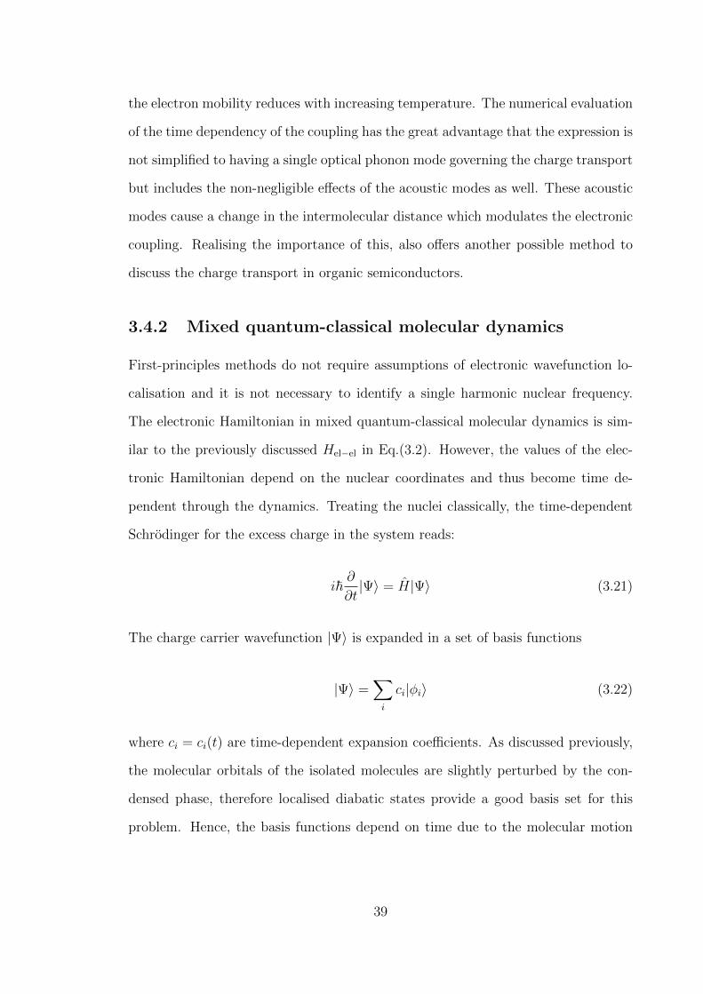
3.4.2 Mixed quantum-classical molecular dynamics
First-principles methods do not require assumptions of electronic wavefunction lo-
calisation and it is not necessary to identify a single harmonic nuclear frequency.
The electronic Hamiltonian in mixed quantum-classical molecular dynamics is sim-
ilar to the previously discussed Hel−el in Eq.(3.2). However, the values of the elec-
tronic Hamiltonian depend on the nuclear coordinates and thus become time de-
pendent through the dynamics. Treating the nuclei classically, the time-dependent
Schrodinger for the excess charge in the system reads:
i~∂
∂t|Ψ〉 = H|Ψ〉 (3.21)
The charge carrier wavefunction |Ψ〉 is expanded in a set of basis functions
|Ψ〉 =∑i
ci|φi〉 (3.22)
where ci = ci(t) are time-dependent expansion coefficients. As discussed previously,
the molecular orbitals of the isolated molecules are slightly perturbed by the con-
densed phase, therefore localised diabatic states provide a good basis set for this
problem. Hence, the basis functions depend on time due to the molecular motion
39

φ = φ(R(t)). By inserting the expression (3.22) into Eq. (3.21) we get
i~dckdt
=∑j
(Hkj − 〈φk|
dφjdt〉)cj (3.23)
Eq. (3.23) can be solved numerically using, for example, the Runge–Kutta algorithm
from which the c(t) values can be obtained.
Adiabatic dynamics (Born–Oppenheimer or Carr–Parinello) are often used and
are standardly available in several quantum chemistry program packages. However,
it uses the assumption that the electronic system remains in the same adiabatic
electronic state throughout the dynamics. As mentioned in the previous section,
this is not necessarily true in organic semiconductors as some coupling values are
small. Therefore, the energy gap between different electronic surfaces is small and
transitions between electronic states need to be incorporated during the dynamics.
Hence, a non-adiabatic molecular dynamics (NAMD) treatment is required.
The simplest NAMD method is to use the classical path method, where the
electron dynamics is done on a previously computed molecular dynamics trajectory.
In this approach, any possible effect of the electron dynamics on the nuclear motion
is completely ignored. However, omitting the feedback from the electron dynamics
to the nuclear structure dissociates the charge from the associated deformation and
give erroneous results. For example, in crystalline semiconductors, the classical path
method may overdelocalise the charge, preventing the formation of a small polaron
in special cases. Therefore, different approaches had to be considered [53].
In the Ehrenfest method, multiple potential energy surfaces are taken into ac-
count. The molecular dynamics happens on a mean field surface that is an average
of these potential energy surfaces with weights proportional to the square of the ex-
pansion coefficient for each electronic state. However, if the potential energy surfaces
refer to very different physical processes the dynamics can fail as the mean field can
represent an unphysical state [54].
40
Surface hopping avoids the problem of mean field approximation. Similarly to the
previous case, there are multiple potential energy surfaces. The nuclear subsystem
is evolving on only one of these potential energy surfaces at a time and the forces
calculated from the charge propagation are fed back to the system. At each molecular
time step, it is checked whether the system has undergone a state switch, in which
case the molecular dynamics continues on another potential energy surface. In this
case, it is a key issue to define such potential surfaces that can adequately describe
the charge carrier transport [55]. While the risk of unphysical states is mitigated
in surface hopping, unlike in the Ehrenfest method, the energy is not automatically
conserved and the energy has to be rescaled at each surface hopping event.
3.5 Conclusion of charge transport methods and
thesis statement
Several charge transport model have been presented here which are used to model
charge transport in organic semiconductors. The band transport and the localised
charge transport methods offer a reasonably simple solution which can be tackled
with the calculation of only a few computationally intensive values, albeit they use
assumptions of localisation and delocalisation which often break down in realistic
systems due to dynamic disorder. The non-local electron-phonon coupling model
and non-adiabatic molecular dynamics do not use any assumptions of localisation
or delocalisation, hence they appear to be more suitable for discussing organic semi-
conductors at room temperature. Non-adiabatic molecular dynamics has the added
benefit that the dynamic and static disorder can be both represented in the diago-
nal and off-diagonal elements of the Hamiltonian, hence it is expected to be general
and applicable even in the special case of fullerenes, where the free rotation of the
molecules at room temperature strongly modulates the coupling, and can be applied
to any general organic semiconducting material. However, using non-adiabatic dy-
41

namic requires the fast evaluation of numerous quantum mechanical properties in
large systems which makes it a computationally intensive method.
Taking the example of fcc C60 where the unit cell contains 4 molecules and taking
a supercell of 3×3×3 for a 1 ns trajectory can give some insight about the behaviour
of the system. Such simulation requires a time resolution finer than the largest
frequency in the system. For example, in the case of describing a C=C stretch this
has to be around 1 fs. Assuming that only nearest neighbours are included there are
108 diagonal and (12×108)/2 non-zero off-diagonal elements in the Hamiltonian and
the same number in the overlap matrix elements. Furthermore, the non-adiabatic
coupling vector also needs to be calculated for 106 snapshots. Whilst the diagonals of
the Hamiltonians can be approximated using a classical approximation by taking the
vertical ionisation energy in the MD, this is not possible for the electronic coupling
matrix elements, the non-adiabatic coupling vector, and the overlap.
The aim of this project is to provide a toolkit for supporting charge transport
models in π-conjugated systems which scales favourably with system size. To this
end, the focus is on the off-diagonal elements of the Hamiltonian, the overlap matrix,
and the non-adiabatic coupling vectors calculated in an appropriately chosen basis
set. In Chapter 5 of this thesis, I will present an efficient method that I have
developed for this purpose. In the following chapter I will present explicit electronic
structure methods for the calculation of electronic coupling that will be used for
calibration of the more cost-effective calculations presented in Chapter 5.
42
4 Benchmark study on the accu-
racy of coupling calculation meth-
ods
As was mentioned in Chapters 2 and 3, the accurate calculation of electronic cou-
plings has an important role in the understanding of charge transport in organic
semiconductors, even more so when the electronic coupling matrix elements are of
a similar order of magnitude as the reorganisation energy. Unlike the diagonal ele-
ments of the Hamiltonian, they cannot be approximated with classical models and
their calculation is often time consuming and therefore size limiting.
Motivated by building accurate transport models, this chapter focuses on the
comparative analysis of different coupling calculation methods which were calculated
within our group and in collaboration with other groups [56]. The results are com-
pared to reference values obtained using high level ab initio methods in combination
with generalised Mulliken–Hush theory (GMHT). The electronic coupling values are
calculated with density functional theory methods: constrained density functional
theory (CDFT), and fragment orbital density functional theory (FODFT). Further-
more, approximate fragment orbital density functional tight binding (FODFTB) is
also compared to these methods.
There are several other models which are not presented here. Time dependent
density functional theory can be used to calculate electronic coupling values. Difley
et al argues that while for the exact density functional the ground state is adiabatic
commonly used approximate functionals often produce diabatic states which can be
43

tested with attachment/detachment analysis [57]. Other methods such as Zerner’s
intermediate neglect of differential overlaps (ZINDO) method has also be used to
calculate the coupling values [46].
The chapter starts with a brief introduction of the underlying theory of each
method and their limitations. Then, a set of systems are introduced which aim to
capture the basic characteristics of organic semiconductors for which the coupling
values are calculated with the listed coupling calculation methods.
The results presented here offer an insight into the varying accuracy and com-
putational demands of the different methods. The calculations were performed on
organic molecules with increasing numbers of heavy atoms, which enabled an anal-
ysis of the feasibility of the different techniques. Alongside the size limitations, the
effect of heteroatoms and the influence of the orientation of the molecules on the
coupling is also tested. The chapter is concluded with the comparison of the com-
putational demands of the methods presented.
4.1 Introduction to electronic coupling calculation
methods
It is worth emphasising the difference between adiabatic and diabatic surfaces which
both have a key role in electronic transitions. Adiabatic states and potential energy
surfaces are created by rigorous application of the Born-Oppenheimer approxima-
tion thus the electronic structure is always smooth and the adiabatic states diagnolise
the Hamiltonian matrix. Diabatic states are localised, chemically intuitive electronic
states which play an important role in charge transport theory. In contrast to the
adiabatic states, in the diabatic case the electronic density does not follow continu-
ously the reaction coordinate of the charge transition. Instead, they preserve their
electronic character uniformly as the nuclear structure changes along the reaction
44
coordinate: a covalent system remains covalent and an ionic system remains ionic
throughout. In the non-adiabatic case the charge transition happens suddenly when
the diabatic states get close to one another, for example when the adiabats show an
avoided crossing (See Panel A Fig 3.1). The diabats do not diagonalise the Hamil-
tonian. The electronic coupling matrix elements can be calculated by taking the
diabatic wavefunctions ψdiaba and ψdiab
b at the crossing of state a and state b and
calculating
Hab = 〈ψdiaba |H|ψdiab
b 〉. (4.1)
There are various ways to construct diabats. Van Voorhis et al. [58] distinguishes
between deductive and constructive methods for obtaining ψdiaba and ψdiab
b . Deductive
methods use adiabats to construct diabatic states.
4.1.1 Generalised Mulliken–Hush theory
Generalised Mulliken–Hush theory (GMHT) is one of the deductive ways for obtain-
ing diabatic states using only adiabatic quantities to describe the adiabatic states
[59, 60, 61]. A generalised derivation can be seen in the works of Creutz et al [62].
The method for the two-state system assumes an orthonormal system in which the
adiabatic wavefunctions are denoted as ψ1 and ψ2 ground state and first excited
state respectively. The diabatic localised states are denoted as φa, for the initial
state, and φb, for the final state. The adiabatic states can be described as a linear
combination of the diabatic states
ψ1 = caφa + cbφb (4.2a)
ψ2 = −cbφa + caφb (4.2b)
45

as the adiabatic states diagonalise the Hamiltonian and the overlap between the two
diabatic states is 0 one can see that
cacb =Hab
∆E12
(4.3)
where ∆E12 is the vertical energy gap between the adiabatic ground state and first
excited state and Hab = 〈φa|H|φb〉 is the electronic coupling between states a and b.
The dipole moment between the ground state and the first excited state, µ12, can be
written as
µ12 = 〈ψ1|r|ψ1〉 (4.4)
It is possible to express µ12 in the diabatic basis set by substituting the expressions
from Eq. (4.2) into Eq. (4.4). The diabats are defined so that the dipole moment
vanishes between the two diabatic states (µab = 〈φa|r|φb〉 = 0)
µ12 = cacb(µbb − µaa) (4.5)
where µaa = 〈φa|r|φa〉 and µbb = 〈φb|r|φb〉 are the dipole moments in the diabatic
states. Using Eq. (4.3) the Eq. (4.5) becomes
µ12 =Hab
∆E12
(µbb − µaa) (4.6)
Now (µbb − µaa) can be expressed in the adiabatic basis set by using Eqs. (4.2)
µ12 =Hab
∆E12
√(µ11 − µ22)2 + 4µ2
12 (4.7)
Thus the electronic coupling according to GMHT is given by
|Hab| =|µ12|∆E12√
(µ11 − µ22)2 + 4µ212
(4.8)
46

In special cases, when the initial and final states are symmetric the adiabatic dipole
moment is µ11 = µ22. Therefore, the equation is simplified to:
|Hab| =1
2∆E12. (4.9)
In summary, this method obtains the diabatic coupling as half of the energy dif-
ference between the ground state and the first excited state ∆E12. Therefore, the
matrix that diagonalises the dipole matrix in the adiabatic basis set can be used
to transform the adiabatic Hamiltonian to the diabatic Hamiltonian. This can be
further generalised to more than two states [63, 64]. The accuracy of the GMHT
results depends on the method which is used to calculate the adiabatic states. High
level ab initio methods (multi-reference and post-Hartree-Fock methods) can be
used to calculate diabatic coupling values by applying the generalised Mulliken–
Hush theory (GMHT) of vanishing transition dipole moments. For example, for
small molecules the adiabatic ground and the first excited states can be calculated
with multi-reference configuration interaction (MRCI) [65] and n-electron valence
state perturbation theory (NEVPT2) [66, 67]. After calculating the dipole matrix
between those states, GMHT can be used to calculate the coupling values [68]. The
method was generalised for multiple sites and can include bulk behaviour [63, 69].
Although these calculations give very accurate results, the drawback is that their
computational costs grow extremely fast with system size. Nevertheless, GMHT is
a useful tool for calculating the coupling and can be used in cases where the po-
larisation effects are significant such as donor-bridge-acceptor systems [70] and to
evaluate experimental spectra [71].
4.1.2 Charge Constrained DFT
While GMHT calculates the coupling deductively from the adiabatic states, there are
several methods to construct the diabatic states directly. For example, constrained
47

DFT (CDFT) obtains the diabatic states by introducing a constraint on the charge
of the donor and the acceptor [58, 72]. In a CDFT calculation, the KS energy
is minimised under the constraint that the charge difference between donor and
acceptor is equal to a specified value (usually +1 or -1 for transfer of a full electron
from donor to acceptor). The restriction is introduced by multiplying the density
ρ(r) with a weight function w(r) which creates a charge difference between the region
where the charge is to be localised and the rest of the space as
Nc =
∫w(r)ρ(r)dr (4.10)
where Nc is the charge difference between the restriction space and the rest of the
space; in this case the donor and the acceptor. Therefore, the task is to minimse
E[ρ] subject to the normalised constraint
0 =
∫w(r)ρ(r)dr−Nc (4.11)
The constraint is added to the energy expression multiplied by a Lagrange multiplier:
W [ρ, Vc] = E[ρ] + Vc
(∫w(r)ρ(r)dr−Nc
)(4.12)
The Kohn–Sham equations then become
(−1
2∆ +
∫ρ(r′)
|r− r′|dr′ + vxc(r) + V w(r)
)ψi = εiψi (4.13)
where vxc(r) is the exchange-correlation functional and ψi are the Kohn–Sham or-
bitals. The expressionW is minimised for given values of V and V is varied iteratively
until the density ρ =∑
i |ψi|2 satisfies Eq. (4.10). Hence, the charge localised (or
diabatic) states obtained from CDFT are adiabatic ground state energies of a KS
Hamiltonian with a modified external potential.
48

The weight function depends on the definition of charge population. In this work,
w(r) is based on the Hirshfeld charge difference [73] between the donor D and the
acceptor A
w(r) =
∑i∈D ρi(r−Ri)−
∑i∈A ρi(r−Ri)∑N
i=1 ρi(r−Ri)(4.14)
where N is the number of atoms in the system. ρi(r − Ri) is the unperturbed
electron density on atom i summed over all Kohn–Sham orbitals and weighted with
the corresponding occupation number nj
ρi(r−Ri) =∑j
nj|ψj(r−Ri)|2 (4.15)
In a dimer system, after obtaining ΨA where the charge is localised on the donor,
ΨB where the charge is localised on the acceptor can be obtained by changing the
constraint Nb = −Nc. Using the constructed diabatic states, the electronic coupling
matrix element can be calculated as HAB = 〈ΨA|H|ΨB〉, where the Hamiltonian is
replaced by the Kohn–Sham Hamiltonian constructed from the orbitals of state A
and state B
H′′ =
EA HAB
HBA EB
(4.16)
where EA = 〈ΨA|HKSA |ΨA〉 and EB = 〈ΨB|HKS
B |ΨB〉 are the energies in the diabatic
states A and B. The off-diagonal elements are
HAB = 〈ΨA|HKSB |ΨB〉 (4.17a)
HBA = 〈ΨB|HKSA |ΨA〉 (4.17b)
Using the fact that the ΨA is the eigenfunction of HKSA , the equations can be trans-
49

formed by adding and subtracting VA∑n
i=1wi(ri)
HAB = SAB〈ΨB|HKSB + VB
n∑i=1
wi(ri)|ΨB〉 − VB〈ΨA|n∑i=1
wi(ri)|ΨB〉 (4.18a)
HBA = SBA〈ΨA|HKSA + VA
n∑i=1
wi(ri)|ΨA〉 − VA〈ΨB|n∑i=1
wi(ri)|ΨA〉 (4.18b)
where SAB = SBA∗ is the off-diagonal element of the overlap matrix between the two
diabatic states. By defining the weight matrix and using its off-diagonal elements
WAB = WBA∗, the expressions in Eq. (4.18) become
HAB = SAB〈ΨB|HKSB + VB
n∑i=1
wi(ri)|ΨB〉 − VBWAB (4.19a)
HBA = SBA〈ΨA|HKSA + VA
n∑i=1
wi(ri)|ΨA〉 − VAWBA (4.19b)
In general, H′′ is not Hermitian, HAB 6= HBA∗, only when the two diabatic states
are degenerate 〈ΨB|HKSB +VB
∑ni=1wi(ri)|ΨB〉 = 〈ΨA|HKS
A +VA∑n
i=1wi(ri)|ΨA〉 and
VB = VA. This is almost never true in practice because of the approximate nature
of the Kohn–Sham Hamiltonian. The off-diagonal element can be approximated by
taking the average off-diagonal value, 12(HAB +HBA). Another option is to describe
the coupling value as the off-diagonal element of the diabatic orthogonal Hamiltonian
H. To this end, ΨA and ΨB can be orthogonalised by being transformed to Ψa and
Ψb which are the eigenfunctions of the weight matrix. The generalised eigenvalue
equation is
WV = SVL (4.20)
Here, W is the weight matrix, L is the diagonal matrix of the eigenvalues of W and
the rows of V are the generalised eigenstates of W, which are very similar to the states
which diagonlise the transition dipole moment vector in generalised Mulliken–Hush
theory but not identical. Once V is calculated, the orthogonal diabatic Hamiltonian
50
can be obtained as
H = V†H′′V (4.21)
and the coupling can be obtained as the off-diagonal element of H. CDFT has been
implemented into plane wave [74] and Gaussian codes [75]. The great benefit of this
method is that it can include interaction with the surroundings [76, 77, 78]. Al-
though constrained DFT is less computationally demanding than high level ab initio
calculations, obtaining converged diabatic states can be computationally costly due
to the possible slow convergence of the Lagrange multiplier [56]. Spin contamination
is also common problem in the CDFT approach.
4.1.3 Fragment orbital DFT
The issues arising from spin contamination and the slow convergence of the Lagrange
multiplier can be avoided when another way of directly constructing localised dia-
batic electronic state, fragment orbital density functional theory (FODFT), is used.
In this case, the diabatic electronic states are constructed from the Kohn–Sham or-
bitals coming from isolated unconstrained DFT calculation on the isolated donor and
acceptor molecules. The separation prevents spurious delocalisation of the electron
which arises from the self-interaction error.
Taking the example of electron transport in a reduced dimer system, let us model
the charge transition from the donor molecule to the acceptor molecule. The initial
state (a) is a charged donor and a neutral acceptor [D− + A]. After the transfer,
the final state b is a charged acceptor and a neutral donor [D + A−]. The coupling
matrix element is calculated by taking the transfer integral between the two states
a and b as
Hab = 〈ψa|H|ψb〉. (4.22)
where ψa and ψb are the wavefunctions of diabatic states a and b. Similarly to the
CDFT method, the exact Hamiltonian is replaced with the Kohn–Sham Hamiltonian
51

constructed from either state a or state b.
Hab = 〈ψa|H|ψb〉 ≈ 〈ψa|HKSb |ψb〉. (4.23)
or
Hba = 〈ψa|H|ψb〉 ≈ 〈ψa|HKSa |ψb〉. (4.24)
It is important to note that, while Hab is approximately the same as Hba for homo-
dimer systems, the difference can be quite significant if the acceptor and the donor
are different molecules. The states a and b are constructed the following way: assum-
ing N electrons on the neutral monomers, each diabatic state representing the dimer
can be regarded as a 2N + 1 electron system. These are expressed as a determinant
built from the Kohn–Sham orbitals of the monomers D− (φD1 , . . . φDN+1) and A−
(φA1 , . . . φAN+1. In practice, the orbitals calculated on the isolated monomers are
concatenated and orthogonalised according to Lowdin and the aforementioned or-
bital subsets are used to construct the diabatic states. An illustration of this can be
seen in Fig. 4.1.
ψa =1√
2N + 1!det(φa1, . . . , φ
a2N+1) =
1√2N + 1!
det(φD1 , . . . , φDN+1, φ
A1 , . . . , φ
AN),
(4.25a)
ψb =1√
2N + 1!det(φb1, . . . , φ
b2N+1) =
1√2N + 1!
det(φD1 , . . . , φDN , φ
A1 , . . . , φ
AN+1).
(4.25b)
Using the fragment orbital wavefunctions from Eq. (4.25a)
Hab ≈ 〈ψa|HKSb |ψb〉 ≈ 〈ψFOa |HKS
b |ψFOb 〉. (4.26)
The expression can be simplified further by taking only the relevant orbitals into
52

Figure 4.1: This figure illustrates the steps of obtaining orbitals for FODFT wavefunction con-struction. The wavefunctions are minimised on the charged isolated donor and acceptor monomers.Then, the obtained Kohn-Sham orbitals are concatenated and orthogonalised.
account
Hab ≈ 〈ψFOa |HKS
b |ψFOb 〉 = 〈φDN+1|HKS
b |φAN+1〉. (4.27)
In summary, when using FODFT the following assumptions are made:
• Only the HOMOs contribute to the electronic coupling: Any contri-
bution from any other part of the wavefunction is omitted.
• The other orbitals are unaffected by the ionisation of the molecule:
Adding or removing an electron alters the electron density and may have an ef-
fect on the other Kohn–Sham orbitals. During the construction of the diabatic
states and Kohn–Sham Hamiltonians, these relaxation effects on the orbitals
are neglected.
53

• All polarisation effects are neglected between the D and A molecules:
The donor and acceptor molecules are separated during the wavefunction op-
timisation. In the bulk, or in a dimer system (e.g. with CDFT), the SCF
optimisation may be affected by the charge and the multipole moments of the
donor. This completely omitted here.
FODFT has been successfully used to analyse C60 [45] and PCBM [49] systems as
well as for biological cofactors [79, 80].
4.1.4 Density functional tight-binding
Density functional tight-binding (DFTB) offers a fast approximate way to calculate
the electronic coupling matrix element. A reference density is obtained as the su-
perposition of neutral atomic densities. The reference density is then expanded as a
Taylor-series and the level of DFTB depends on the maximum order of the Taylor-
series components. If only the first order components are used (DFTB1) there is
no deviation from the reference density; therefore this method is not used. The
most common levels of theory are DFTB2 [81] and DFTB3 [82]. If one describes the
Kohn–Sham equations as
h0ϕi =
[−1
2∆ + Veff
]ϕi = εiϕi (4.28)
where the effective potential is
Veff = Vext + Vee + Vxc (4.29)
and its components are the electron-nuclei interaction Vext, the electron-electron
interaction Vee, and the exchange-correlation interaction Vxc.
54
These are described as
Vext = −N∑j=1
Zj|r−Rj|
r (4.30a)
Vee =
∫ρ(r′)
|r− r′|dr′ (4.30b)
Vxc =δExc
δρ(4.30c)
Here, ρ =∑n
i=1 ϕ∗iϕi is the electron density, n is the number of electrons; Rj, Zj
and N are the position, the charge and the total number of the nuclei respectively;
and Exc[ρ] is the exchange-correlation energy. The total energy expression is thus
Etot =n∑i
〈ϕi|h0|ϕi〉 −∫Veeρdr + Exc[ρ]−
∫δExc
δρρdr + Enn (4.31)
where Enn is the nuclear repulsive interaction Enn =∑
j>lZjZlRjl
and Rjl = |Rj −Rl|.
If Eq. (4.31) is expanded into a Taylor-series around a reference density ρ0 where
ρ = ρ0 + δρ the first order terms vanish. The second order terms are non-zero for
two components Exc[ρ] and∫Veeρdr.
Etot =n∑i
〈ϕi|h0|ϕi〉 −∫Veeρ
0dr + Exc[ρ0]−
∫δExc
δρ
∣∣∣ρ0ρ0dr + Enn
+
∫ ∫ (1
|r− r′|+δ2Excδρδρ′
∣∣∣ρ0
)δρδρ′drdr′ (4.32)
where the zeroth order components are often summarised in the repulsive potential
Vrep [83]:
Vrep =
∫Veeρ
0dr + Exc[ρ0]−
∫δExc
δρ
∣∣∣ρ0ρ0dr + Enn (4.33)
The reference density ρ0 can be written as a superposition of atomic densities ρ0(r) =∑Ni ρ
0i (r) and the potentials can be written as the superposition of atomic potentials
Vee(r) =∑N
i Veei(r). The second order energy term is usually approximated with
55
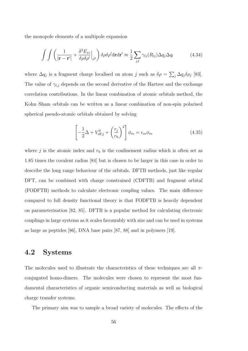
the monopole elements of a multipole expansion
∫ ∫ (1
|r− r′|+δ2Excδρδρ′
∣∣∣ρ0
)δρδρ′drdr′ ≈ 1
2
∑j,l
γlj(Rlj)∆qj∆ql (4.34)
where ∆qj is a fragment charge localised on atom j such as δρ =∑
j ∆qjδρj [83].
The value of γl,j depends on the second derivative of the Hartree and the exchange
correlation contributions. In the linear combination of atomic orbitals method, the
Kohn–Sham orbitals can be written as a linear combination of non-spin polarised
spherical pseudo-atomic orbitals obtained by solving
[−1
2∆ + V 0
eff,j +
(rjr0
)2]φm = εmφm (4.35)
where j is the atomic index and r0 is the confinement radius which is often set as
1.85 times the covalent radius [84] but is chosen to be larger in this case in order to
describe the long range behaviour of the orbitals. DFTB methods, just like regular
DFT, can be combined with charge constrained (CDFTB) and fragment orbital
(FODFTB) methods to calculate electronic coupling values. The main difference
compared to full density functional theory is that FODFTB is heavily dependent
on parameterisation [82, 85]. DFTB is a popular method for calculating electronic
couplings in large systems as it scales favourably with size and can be used in systems
as large as peptides [86], DNA base pairs [87, 88] and in polymers [19].
4.2 Systems
The molecules used to illustrate the characteristics of these techniques are all π-
conjugated homo-dimers. The molecules were chosen to represent the most fun-
damental characteristics of organic semiconducting materials as well as biological
charge transfer systems.
The primary aim was to sample a broad variety of molecules. The effects of the
56

number of double bonds and the various sizes and shapes of π-conjugated molecules
were considered, as well as the effects of heteroatoms in the system and deviation
from perfect stacking.
The size of the molecules range from small to medium sized. The minimum size
was set by the criterion that the molecule had to form a stable anion. To this end,
the individual monomers had to have a positive vertical electron attachment (VEA)
energy when tested with PBE [89] and aug-cc-pVTZ basis set [90]. Although the
general idea was to use high level ab initio calculations as reference such as MRCI+Q,
the lower limit of stable anions eliminated small molecules such as ethylene and
benzene, therefore other reference methods had to be chosen.
The upper limit of the size of the molecules was set by the feasibility of high-level
ab initio calculations. In Ref [68], the relatively small size of the molecule (rang-
ing in size from acetylene to benzene) permitted the application of multi-reference
configuration interaction (MRCI) and n-electron valence state perturbation theory
(NEVPT2). Due to the relatively large size of the molecules, the spin component
scaled approximate coupled cluster method (SCS-CC2) was chosen as the reference
calculation method. The set consisted of a series of acenes, and perylene which were
used to test the effect of the increasing conjugation length in pure hydrocarbons.
The acenes ranged from anthracene to pentacene as neither benzene nor naphtha-
lene formed a stable anion. In fact, the smallest acene to bind an electron (VEA=0.64
eV) was anthracene (See Fig. 4.2). The effect of the heteroatoms in the system was
tested with medium sized molecules including perfluorinated anthracene, where all
hydrogens are replaced with fluorine atoms, porphin, and perylene-diimide. These
D2h molecules form the HAB7- data set.
Three further molecules were considered to be included in the comparison: coronene
(D6h), triphenylene (D3h), and the smallest fullerene C20 (D2h due to Jahn–Teller
distortion). While coronene and tripheylene have degenerate LUMO and LUMO+1,
C20 has quasi-degenerate LUMO and LUMO+1. These degenerate states cannot be
57

Figure 4.2: The seven molecules which were stacked to assess the accuracy of CDFT/X, FODFT,FODFTB coupling calculation methods against GMHT+SCS-CC2 at distances ranging from 3.5to 5.0 A. In addition, six randomly oriented anthracene pairs were also used to assess the effectsof random orientation on the coupling values.
58
treated with ROHF+SCS-CC2 and these molecules are too large for multi-reference
methods. Although quasi-degenerate C20 was converged with ROHF the T1 am-
plitudes [91] were much larger than for the rest of the systems (0.035). The same
state could not be obtained with CDFT, FODFT, and FODFTB, with CDFT hav-
ing serious convergence issues when only generalised gradient approximation (GGA)
exchange was used [89].
The effects of the relative orientation were tested with randomly orientated an-
thracene dimers. These were the only systems which were not perfectly symmetric.
Although the method is fully applicable for hetero-dimers symmetry was crucial
for the computationally intensive reference method and combining anthracene with
another molecule would have been computationally even more intensive.
4.3 Simulation details
The coordinates for the coupling calculation were constructed in the following way.
The neutral monomer structures were optimised using standard DFT calculations
with the BP86 functional [92, 93], in def2-TZVP basis set [94, 95] and resolution
of identity approximation [96, 97] with the Turbomole package [98]. The SCF en-
ergies were converged to 10−7 a.u. while the electronic gradient convergence crite-
rion was set to 10−4 a.u. An enlarged DFT integration grid (m4) was used. After
minimisation the frequency calculations (of the same level of theory as the energy
optimisation) showed that all normal modes were positive. The symmetric dimer
constructions were done by replicating the optimised monomer structure along the
axis perpendicular to the plane of conjugation.
As it is mentioned in our publication [56], reference value calculations were cal-
culated in our group by Adam Kubas using the generalised Mulliken–Hush theory.
All systems except for the randomly oriented anthracene pairs consisted of symmet-
ric homo-dimers hence Eq. (4.9) was used. In the randomly oriented anthracene
59

cases, the more general Eq. (4.8) was used. The ground and the first excited state
were calculated with the spin component scaled approximate coupled cluster method
[99, 100] based on orbitals calculated with restricted open-shell Hartree–Fock method
(ROHF). The ROHF calculations helped to prevent spurious spin-contamination
which was present in UHF calculations. The T1 tests [91] showed values of |t1|/√N
smaller than 0.02 for most systems and smaller than 0.025 for all systems. Some of
these values were slightly larger than the rule of thumb (0.02) as reported in Ref.
[101]. However, this was not a problem in Ref [68] where the T1 diagnostic results
for the UHF/SCS-CC2 results for the systems in Ref [68] gave values between 0.02
and 0.03 while still approximating the MRCI+Q results well. In order to improve
performance, the spin component scaling was done by using the same (css = 1/3)
and opposite spin-component factors (cos = 6/5) on the spin components of the
Jacobian matrix used for calculating the excitation [102]. Resolution of identity ap-
proximation was used with an auxiliary basis set according to Ref [103]. The basis
set for heavy atoms was aug-cc-pVTZ [90] and the for hydrogen was cc-pVDZ [104],
similarly to those in Ref [68].
I contributed CDFT and FODFT calculations to this benchmark study. The
calculations were done using the CPMD plane wave package [105]. The simulation
details were identical to those in Ref. [68]. In the CDFT calculations, the Lagrange
multiplier was optimised until the Hirshfeld charge difference between the donor
and the acceptor monomers was 1e to within a tolerance of 5 × 10⁻⁵ e. All atoms
of the donor and acceptor monomers were included. All CDFT calculations were
done in vacuo using the PBE functional [89]. The influence of exact exchange was
tested by partially replacing the GGA exchange with different percentages of (ex-
act) Hartree–Fock exchange (HFX). These calculations are labelled as “CDFT/X”,
where X denotes the percentage of HFX. Since the code uses a plane wave basis
set in isolated system calculations, the effect of the images has to be decoupled
from the system. It is also important that the chosen unit cell (box size) is large
60

enough to allow the wavefunction to converge to zero at the box boundaries. A
minimum vacuum gap of 4 A on each side of the molecule proved to be enough;
further increment of the box size (and the vacuum gap) did not change the coupling
values by more than 0.2 meV. Troullier–Martins pseudopotentials [106] were used
to replace core electrons. Therefore, in addition to the 4 A vacuum gap, the box
was also ensured to be larger than twice the system size (approximating the size
with the van der Waals radius). The basis set was terminated at 80 Ry reciprocal
space plane wave cut-off for the Kohn–Sham orbitals in order to fulfill the size crite-
ria for the Martyna–Tuckerman Poisson solver [107]. A decreased cut-off was used
for exact exchange density calculations. The dimers were centred in a rectangular
box. FODFT(2N + 1) calculations were performed with the same parameters as
CDFT, using the unmodified PBE functional. The orbitals were orthogonalised us-
ing the Lowdin orthogonalisation method. The coupling values were calculated with
both possible Kohn–Sham Hamiltonians, HKSb (Hab) and HKS
a (Hba), depending on
which orbital is excluded when constructing the operator (see Fig 4.1). Finally, the
obtained couplings Hab and Hba were averaged.
FODFTB calculations were performed by our collaborators using their custom
written code. To capture the intermolecular interactions, in addition to the halorg-
0-1 DFTB parameters [81, 108] a second less confined parameter set was used as in
Ref [68] with additional parameters for fluorine. The calculations were done with a
total energy convergence criterion of 10−7 a.u. The basis set was an effective double-
zeta description [81], the confinement in Eq. (4.35) was 8 a.u. for the wavefunction
and ∞ for the density for all atoms.
While GMHT and FODFTB values were calculated in a Gaussian basis, set
CDFT and FODFT values were calculated in plane wave basis set. The basis set,
however, does not have a significant effect on the coupling Kubas et al compared
the methods with different basis set in Ref [68]. Moreover Gaussian basis set CDFT
code implemented in the deMon2k program package and the plane wave CDFT code
61
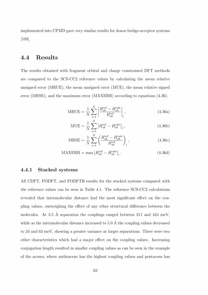
implemented into CPMD gave very similar results for donor-bridge-acceptor systems
[109].
4.4 Results
The results obtained with fragment orbital and charge constrained DFT methods
are compared to the SCS-CC2 reference values by calculating the mean relative
unsigned error (MRUE), the mean unsigned error (MUE), the mean relative signed
error (MRSE), and the maximum error (MAXERR) according to equations (4.36).
MRUE =1
N
N∑i=1
∣∣∣∣Hrefab −Hcalc
ab
Hrefab
∣∣∣∣i
, (4.36a)
MUE =1
N
N∑i=1
∣∣Hrefab −Hcalc
ab
∣∣i, (4.36b)
MRSE =1
N
N∑i=1
(Hrefab −Hcalc
ab
Hrefab
)i
, (4.36c)
MAXERR = max∣∣Href
ab −Hcalcab
∣∣i. (4.36d)
4.4.1 Stacked systems
All CDFT, FODFT, and FODFTB results for the stacked systems compared with
the reference values can be seen in Table 4.1. The reference SCS-CC2 calculations
revealed that intermolecular distance had the most significant effect on the cou-
pling values, outweighing the effect of any other structural difference between the
molecules. At 3.5 A separation the couplings ranged between 311 and 424 meV,
while as the intermolecular distance increased to 5.0 A the coupling values decreased
to 24 and 63 meV, showing a greater variance at larger separations. There were two
other characteristics which had a major effect on the coupling values. Increasing
conjugation length resulted in smaller coupling values as can be seen in the example
of the acenes, where anthracene has the highest coupling values and pentacene has
62

the lowest when compared at the same distance. This phenomenon becomes more
prominent as the separation increases. Even more significant coupling reduction can
be introduced through electron withdrawing groups: perfluorinated anthracene had
26% smaller coupling at 3.5 A and 55% smaller at 5.0 A compared to anthracene.
Similarly, perylene-diimide had 12% smaller coupling than perylene. It is assumed
that both the electron withdrawing groups and the increased conjugation length
reduces the couplings by introducing a more stable anion.
Inclusion of exact exchange proved to be crucial in CDFT calculations. With-
out Hartree–Fock exchange, this approximation is often subject to spin contamina-
tion and hybrid functionals are needed to aid the localisation of the diabatic states
[68]. As expected, CDFT/0 overestimated the coupling significantly (MRUE 60.8%),
however increasing the percentage of Hartree–Fock exchange decreased the coupling.
Introducing 25% exact exchange improved the results but the list value of the error
was still large. Interestingly, using range-separated HSE06 functional did not have
any advantage and the obtained errors were very similar to PBE0 which also con-
tains 25% exact-exchange. The best estimate for the coupling values was given by
CDFT with 50% Hartree–Fock exchange with a MRUE of only 8.2%.
Although FODFT and FODFTB are more approximate than CDFT as they omit
polarisation effects between the donor and the acceptor, they gave slightly better
results than CDFT/0 with PBE. This clearly shows that in the case of CDFT/0,
over-delocalisation outweighs the advantage of higher level theory. In fact, in terms
of MRUE the FODFT results are closer to the CDFT/25 results. FODFTB gives
larger errors than FODFT with 53.5 % MRUE.
Linear scaling improved the results significantly for all presented methods. The
scaled errors can be seen in Table 4.2 and on Panel B of Fig 4.3 the scaled re-
sults are marked with the ‘s’ prefix. The lines were fitted with the least squares
method and the R2 values were 0.9990, 0.9996, 0.9988, 0.9997, 0.9985, and 0.9879
for CDFT/0, CDFT/25, CDFT/50, HSE06, FODFT, and FODFTB respectively.
63
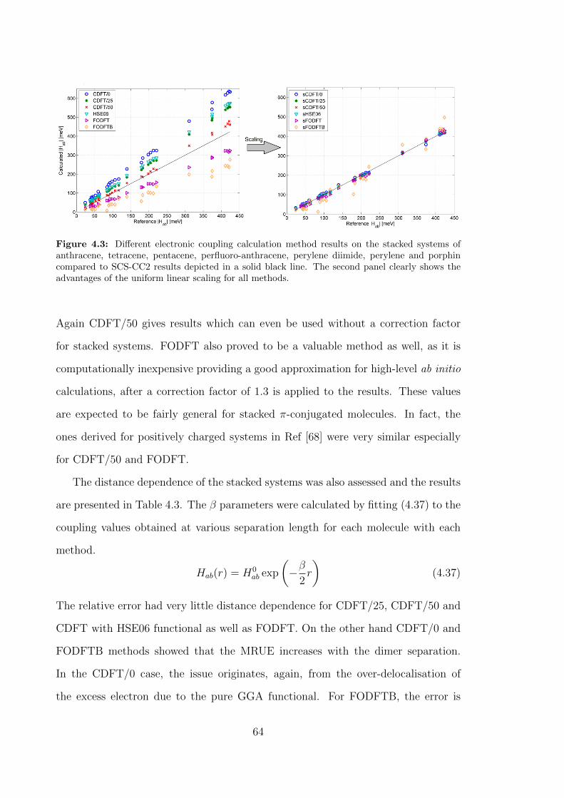
Figure 4.3: Different electronic coupling calculation method results on the stacked systems ofanthracene, tetracene, pentacene, perfluoro-anthracene, perylene diimide, perylene and porphincompared to SCS-CC2 results depicted in a solid black line. The second panel clearly shows theadvantages of the uniform linear scaling for all methods.
Again CDFT/50 gives results which can even be used without a correction factor
for stacked systems. FODFT also proved to be a valuable method as well, as it is
computationally inexpensive providing a good approximation for high-level ab initio
calculations, after a correction factor of 1.3 is applied to the results. These values
are expected to be fairly general for stacked π-conjugated molecules. In fact, the
ones derived for positively charged systems in Ref [68] were very similar especially
for CDFT/50 and FODFT.
The distance dependence of the stacked systems was also assessed and the results
are presented in Table 4.3. The β parameters were calculated by fitting (4.37) to the
coupling values obtained at various separation length for each molecule with each
method.
Hab(r) = H0ab exp
(−β
2r
)(4.37)
The relative error had very little distance dependence for CDFT/25, CDFT/50 and
CDFT with HSE06 functional as well as FODFT. On the other hand CDFT/0 and
FODFTB methods showed that the MRUE increases with the dimer separation.
In the CDFT/0 case, the issue originates, again, from the over-delocalisation of
the excess electron due to the pure GGA functional. For FODFTB, the error is
64

due to the minimal basis set used for the calculations, which fails to fully describe
the more diffuse singly occupied molecular orbitals of the anions despite special
optimisation. Furthermore, the coupled orbitals were virtual orbitals and therefore
distance dependency could not be reproduced. As a consequence, the FODFTB
electronic couplings decrease too quickly with dimer separation which results in a β
parameter which overestimates the ab initio results by 26%.
4.4.2 Randomly oriented anthracene molecules
As shown for the stacked systems, although there are small differences between the
equidistant coupling values for different molecules, they are in general rather sim-
ilar. To test the effect of broken symmetry, a few randomly oriented dimers were
used. Since the reduction of symmetry from D2h to C1 increased the computational
demands significantly, the smallest possible system: a dimer of anthracene molecules
was chosen for this study. Even then, out of the fifteen possible conformations only
six dimers converged as the system size was too large to converge into a shallow min-
imum within a reasonable computational time. The SCS-CC2 reference calculations
were compared to CDFT/50, CDFT/0, FODFT and FODFTB results. The scaled
results, corrected with the factors from Table 4.2, are presented in Table 4.4. Just
like in the stacked case, the separation of the nearest atoms of the two monomers r
had a significant effect on the couplings, which decreased with increasing interatomic
distance. However, intermolecular distance is not the only factor which affects the
coupling values. As large π-conjugated molecules have a complicated nodal struc-
ture, imperfectly stacked structures have radically reduced coupling values as was
shown in Ref [49]. This also arises partly from the fact that perfectly stacked sys-
tems have the lowest overall distance. A similar effect can be observed in the work
of Breuer et al. where the main factor affecting the coupling values is the type of
stacking [79]. This is why configurations 2 to 4 have couplings which are an order of
magnitude smaller than their perfectly stacked counterparts at 5 A (See Fig. 4.4).
65

Even for the last two entries in Table 4.4 where the shortest interatomic distance is
Figure 4.4: Randomly oriented anthracene pairs used for testing the effect of orientation. Thesestructures are quite different from the perfectly stacked systems presented above. The numbersnext to the panels refer to the ID numbers presented in Table 4.4.
66

much less than 3.5 A the overlap is around the same order of magnitude as it was
for the 5 A separation perfectly stacked anthracenes. This also puts the accuracy of
the methods to question for these rotated structures as couplings below 5 meV are
subject to significant numeric noise. Nevertheless, despite the relatively large noise
the trends of the coupling values for different methods are preserved. Also, similarly
to the stacked cases for dimer 5 and 6, FODFT underestimates Hab while CDFT
overestimates it. It is interesting to see that the errors with CDFT/50 are larger
than in the stacked case (200 meV while reference is 91 meV). This is probably due
to the very short carbon-hydrogen interatomic distance where the over-delocalisation
is a more significant issue which can be remedied with increased percentage of HFX.
At such small distances, the weighting function can also have an effect on the CDFT
results [72, 74].
4.5 Computational demands
Several different methods were presented in the previous section which gave different
errors and it was shown that CDFT/50 approximates the reference values best.
However, it is interesting to see how the computational demands compare to the
errors. As mentioned earlier, the coupling calculation can act as a bottleneck when
charge transport models are used for extended systems. Fig. 4.5 shows the CPU time
with different methods on different stacked systems and the corresponding error.
The size limitation of SCS-CC2 has been discussed earlier and it is not applicable
for any system larger than a dimer. While CDFT with 50% exact exchange gives
very good results and can be applied to larger molecules than SCS-CC2, it is still
not feasible for systems as large as a C60 dimer. Furthermore, while couplings for a
single dimer consisting of small molecule organic semiconductors such as rubrene or
pentacene are possible, a statistically significant system of several molecules would
be impossible with CDFT and HFX. FODFT requires less computational time and
67
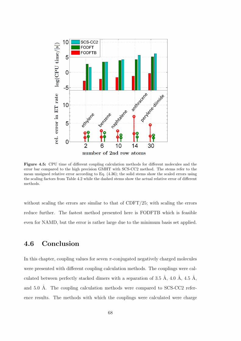
Figure 4.5: CPU time of different coupling calculation methods for different molecules and theerror bar compared to the high precision GMHT with SCS-CC2 method. The stems refer to themean unsigned relative error according to Eq. (4.36); the solid stems show the scaled errors usingthe scaling factors from Table 4.2 while the dashed stems show the actual relative error of differentmethods.
without scaling the errors are similar to that of CDFT/25; with scaling the errors
reduce further. The fastest method presented here is FODFTB which is feasible
even for NAMD, but the error is rather large due to the minimum basis set applied.
4.6 Conclusion
In this chapter, coupling values for seven π-conjugated negatively charged molecules
were presented with different coupling calculation methods. The couplings were cal-
culated between perfectly stacked dimers with a separation of 3.5 A, 4.0 A, 4.5 A,
and 5.0 A. The coupling calculation methods were compared to SCS-CC2 refer-
ence results. The methods with which the couplings were calculated were charge
68

constrained density functional theory with different exchange correlation function-
als, fragment orbital DFT, and fragment orbital density functional tight-binding.
CDFT with 50% exact exchange had the smallest relative error compared to the
reference values, while decreasing proportion of exact exchange increased the errors
significantly. In fact, the errors for CDFT/0 were much larger (MRUE= 60.8%)
than in the positively charged case [68] (MRUE= 38.7%) which is due to the more
prominent over-delocalisation in the anionic system. Since CDFT with 50% exact
exchange proved to be the best approach for both oxidised [68] and reduced example
molecules it is expected to be transferable to other π-conjugated systems. Neverthe-
less, further generalisation should be avoided as the recommended HFX percentage
may vary for different systems. McKenna et al. found that 25% exchange worked
best for electron tunneling between lattice defects in MgO [76, 77]. Interestingly,
range separation offered no clear advantage for these systems: the HSE06 functional
yielded very similar results to to CDFT/25 (PBE0).
Slightly faster than CDFT+PBE, FODFT+PBE also matched the reference val-
ues better as over-delocalisation was prevented by the separation of dimers. The
relative error improved further when uniform scaling factors were applied to the
results. For FODFT the scaling factor was very similar in both the reduced and
oxidised cases (around 1.3) [68] and the MRUE was reduced from 27.9% to 5.9%
overall. The scaled FODFT+PBE results gave similar errors to CDFT/50 at the
fraction of the computational cost. FODFTB was clearly the fastest listed method
but the errors were also larger compared to other methods. This is due to the mini-
mal basis set and the virtual orbitals used to construct the LUMO for the coupling
calculation. Yet, a uniform scaling factor improves the errors significantly.
Finally, the results for the randomly oriented anthracene dimers suggest that
all approximate methods should be used with caution when small coupling values
are calculated. Couplings lower than 5 meV were not reproduced as well as higher
coupling values and the methods show larger variance when compared with the
69
randomly oriented thiophenes [68].
Although the data set was small, the transferability of the method is expected to
be good. For example, removing any molecule type from the set causes the MRSE
to change by 1% or less. The error is arguably better represented in the context
of the non-adiabatic electron transfer rate. Taking the example of using coupling
values with Marcus theory, the electronic coupling is an external factor in the rate
expression k ∝ H2ab. Hence, if the MRUE of the coupling is 20% the MRUE of
the rate is 40% provided that the activation energy can be obtained accurately.
This means that all methods predict the Marcus rate with less than 60% relative
error. Of course the accuracy of the rate is subject to the accurate calculation of the
reorganisation energy and the driving force.
70

Table 4.1: Electronic coupling matrix element values for the negatively charged symmetric per-fectly stacked dimers of anthracene, tetracene, pentacene, perfluoro-anthracene, perylene-diimide,perylene and porphin at d separation calculated with SCS-CC2+GMHT, CDFT/X, FODFT, andFODFTB methods for the HAB7- set, where X denotes the percentage of Hartree–Fock exchange.All coupling values are in meV. The error values for each method were calculated according to Eqs.(4.36) using SCS-CC2+GMHT results as reference values.
System d [A] Ref CDFT/0 CDFT/25 CDFT/50 HSE06 FODFT FODFTB
anthracene
3.5 421.1 637.0 555.4 479.2 573.1 316.9 237.84.0 212.3 324.5 256.6 227.8 282.8 147.3 98.84.5 106.1 169.4 129.5 113.1 144.1 68.0 39.45.0 52.3 87.9 65.8 58.0 74.5 30.7 14.8
tetracene
3.5 417.2 628.8 548.3 466.0 568.2 322.9 242.94.0 204.3 313.1 259.4 213.8 273.3 149.2 101.64.5 97.9 160.8 127.1 102.4 135.4 69.2 40.85.0 45.4 81.5 62.5 50.4 67.5 32.5 15.5
pentacene
3.5 411.0 618.3 539.4 451.3 560.6 323.2 243.94.0 198.0 303.0 250.1 202.4 264.2 148.5 102.74.5 92.4 154.0 120.1 95.1 129.3 68.5 41.45.0 41.0 77.7 58.2 45.7 63.1 32.0 15.8
perfluoro-anthracene
3.5 310.9 479.6 409.5 349.7 423.0 236.1 198.44.0 139.1 227.2 183.4 152.7 192.7 101.0 80.94.5 59.9 107.9 83.3 68.5 87.9 44.0 31.95.0 24.0 49.6 37.5 30.6 39.6 18.7 12.4
perylene-diimide
3.5 373.8 541.8 484.0 417.7 504.1 285.1 227.04.0 179.2 261.0 222.7 187.4 235.4 130.5 94.14.5 84.1 131.2 107.9 89.2 115.1 60.9 37.55.0 38.0 65.1 52.8 44.0 56.1 29.1 14.4
perylene
3.5 423.7 633.7 553.7 460.7 574.7 324.6 236.34.0 220.7 324.5 272.1 222.7 286.2 156.4 98.54.5 116.6 174.0 140.8 114.1 149.8 77.0 39.35.0 62.8 94.4 75.4 61.1 80.6 39.0 15.0
porphin
3.5 374.5 577.7 496.3 408.5 516.4 288.5 216.04.0 182.9 285.0 231.7 184.8 244.3 131.1 88.74.5 89.0 146.2 111.9 87.3 119.7 59.8 34.75.0 44.1 74.7 55.1 42.7 58.7 28.1 13.2
Errors
MUE [meV] 96.7 53.3 15.0 64.2 46.5 85.3MAXERR [meV] 215.9 134.3 58.1 152.0 104.2 187.4MRSE [%] 60.8 30.7 7.5 38.1 -27.9 -53.5MRUE [%] 60.8 30.7 8.2 38.1 27.9 53.5
71

Table 4.2: Revisited Hab errors after uniform linear scaling is applied to all approximate couplingvalues compared to SCS-CC2 reference values for the stacked systems. The prefix ‘s’ refers to thescaled values.
Method Scaling factor MUE [meV] MRSE [ % ] MRUE [ % ] MAX [meV]sCDFT/0 0.660(0.004) 5.9 6.1 7.3 16.2sCDFT/25 0.768(0.003) 3.9 0.4 3.8 11.7sCDFT/50 0.915(0.006) 6.2 -1.7 4.9 17.3sHSE06 0.738(0.002) 3.2 1.9 3.8 9.6sFODFT 1.325(0.010) 7.0 -4.4 5.9 17.2sFODFTB 1.795(0.038) 21.6 -15.4 19.5 47.7
Table 4.3: Distance dependence of the coupling values according to Eq. (4.37) with the different
coupling calculation methods. All β values are in A−1
. The error values with respect to SCS-CC2+GMHT reference values were calculated with Eqs. (4.36).
System Ref CDFT/0 CDFT/25 CDFT/50 HSE06 FODFT FODFTB
anthracene 2.78 2.64 2.77 2.81 2.72 3.11 3.70
tetracene 2.96 2.72 2.90 2.97 2.84 3.07 3.67pentacene 3.07 2.76 2.96 3.05 2.91 3.08 3.65perfluoro-anthracene
3.41 3.02 3.18 3.24 3.15 3.38 3.70
perylene-diimide
2.55 2.54 2.66 2.70 2.62 2.83 3.68
perylene 3.05 2.82 2.95 3.00 2.92 3.05 3.69porphin 2.85 2.72 2.93 3.01 2.89 3.10 3.72
Errors
MUE [A−1
] 0.21 0.10 0.08 0.12 0.15 0.74
MAXERR [A−1
] 0.39 0.23 0.17 0.26 0.33 1.13MRSE [%] -6.8 -1.3 0.8 -2.7 5.0 25.8MRUE [%] 6.8 3.3 2.9 3.9 5.3 25.8
Table 4.4: Coupling results for the randomly oriented anthracene dimers. d marks the closestC-C distance between the dimers. All coupling values are in meV. The mean unsigned error iscalculated according to Eq. (4.36) using the SCS-CC2 coupling values as reference.
Dimer ID d [A] Ref sCDFT/0 sCDFT/50 sFODFT sFODFTB
1 5.46 0.0 0.9 0.7 1.3 0.12 4.79 2.6 8.7 5.3 5.7 3.33 4.59 1.7 6.0 4.6 5.6 2.04 3.52 2.3 0.9 2.7 2.8 0.35 2.24 46.4 174.3 73.6 31.3 27.36 2.14 91.5 287.7 200.6 70.6 52.3
MUE [meV] 56.2 23.8 7.5 10.2 12.3
72

5 Fast Analytic Overlap Method
In this chapter, I will focus on the calculation of the off-diagonal elements of the elec-
tronic Hamiltonian in the diabatic representation (Hab). The efficient calculation of
these elements is an important step towards mixed quantum-classical molecular dy-
namics providing the quantum mechanical components in the model: the electronic
Hamiltonian, the overlap matrix, and the non-adiabatic coupling vector elements.
First, I will describe my theoretical work towards an ultra fast yet accurate calcu-
lation of overlap matrix elements where the electronic coupling matrix elements are
approximated as being proportional to the electronic overlap of the singly occupied
molecular orbitals. Here, I will emphasise how the reduction of the basis set affects
the accuracy and the computational costs of the calculations. The details of the
semi-empirical parameter derivation to approximate the Hamiltonian off-diagonal
elements are also discussed. A broad selection of structures are used to fit the pa-
rameters using fragment orbital DFT for reference calculations. At the end of the
section the derived parameters are tested against independent calculations. The
following section discusses the application of the method on heme compounds con-
taining transition metals and tackles the issue of how the method can be used in
molecular dynamics. Finally, I present the details of how the overlap method can be
used to approximate the non-adiabatic coupling vector (NACV) elements.
Several semi-empirical methods were presented in Chapter 3 but the computa-
tional costs of even the fast FODFTB method scale unfavourably with molecule
size to be able to use them for non-adiabatic molecular dynamics in large condensed
phase systems [48]. An even faster method can be introduced by neglecting all of the
73

four-electron integrals and using the proportionality between the electronic coupling
and the overlap integrals to approximate Hab as
Hab = CSab. (5.1)
This ansatz is similar to the idea of Huckel theory [110]. However, while the latter was
originally used to describe Hab between atom-centred orbitals of a single molecule
here, Hab refers to the electronic coupling between molecular orbitals on different
molecules [110]. The relation (5.1) has been tested on donor-acceptor pairs of DNA
bases [111], acenes [112], and fullerenes [48], and it was found to give an excellent
approximation for charge transport, with a proportionality constant of C = 14 eV
[48]. It remains unclear, however, if C has to be reparameterised for every single
donor-acceptor system or if Eq. (5.1) can be generalised to a large class of OSC
materials described by a single value for C.
The main requirement to be able to apply non-adiabatic molecular dynamics on
realistic (large) organic semiconducting systems is to be able to calculate the Hamil-
tonian and overlap matrices in an efficient way. For this purpose, we replace the di-
abatic state wavefunction by the highest singly occupied molecular orbital (SOMO).
Similarly to the FODFT method the wavefunction of the isolated molecule was used
for the calculations omitting any kind of polarisation effects of the environment. This
means that only one self-consistent field calculation is needed from which the wave-
function is determined. This wavefunction is later reconstructed for every molecule
forming the bulk and for every molecular dynamics snapshot.
The key for minimising the computational requirements of calculating the overlap
is the choice of an optimal basis set to describe the SOMO. This basis set has to
be as small as possible yet give results which are in good accordance with overlap
values calculated with much larger basis sets. To this end, the SOMO was expanded
in the minimum Slater type valence orbital basis set (STO: 1s for H 2s; 2p for C,
74

N, O; and 3s, 3p for S). For improved computational time, further reduction of the
basis set was considered. Since organic semiconductors are almost exclusively π-
conjugated molecules and these delocalised π-orbitals usually dominate the SOMO
of the molecules, the effect of omitting pσ and s components has been studied and
is presented later. The overlap with these projected orbitals is
Sab ≈ Sab = 〈φ′NA |φ′ND〉 (5.2)
where Sab is the overlap of the SOMOs of the donor and the acceptor in the full SCF
basis set and Sab is the overlap of the SOMOs in the reduced basis set. Eq. (5.2)
was calculated using the analytic integral formulae published by Mulliken [113].
With these formulae, the overlap of Slater orbitals with different quantum numbers
at different separation can be calculated. This reduced basis set and the integral
formulae allow a very fast overlap calculation in terms of atomic orbital overlaps
between a relatively small number of orbitals which will be compared to the other
methods in Fig 4.5.
The final question was how to parameterise Eq. (5.1) to give the best possible
result. For this reason, several reference calculations were done using the DFT
method on a training set of π-conjugated donor-acceptor systems. The derived
parameters were then tested on π-conjugated molecules outside the training set.
I found that Eq. (5.1) with a single parameter C can describe well the electronic
coupling of all molecules investigated, but only if the exponents of the minimum
STO basis set are properly chosen. This led to a speed-up of approximately 6 orders
of magnitude compared to DFT calculations, with little loss of accuracy [114].
75

5.1 Theory
The overlap and the electronic coupling Hab are calculated between the diabatic elec-
tronic wavefunctions for the initial and final electron transfer (ET) states, referred
to as |ψa〉 and |ψb〉. If the correlation between the overlap and electronic coupling
stands it should be valid for any given geometry of a donor-acceptor pair and for a
wide range of π-conjugated donor and acceptor molecules. Depending on the level
of theory, calculation of the exact overlap can be computationally demanding: if one
wants to include bulk behaviour, the diabatic wavefunctions can be approximated
by Kohn–Sham determinants obtained from charge constrained DFT calculations
(Refs [68, 74, 115, 116]). Therefore, several approximations were applied to speed
up the calculation of Sab. Firstly, similarly to FODFT it is assumed that the ET is
mediated by only two orbitals, the SOMO of the isolated reduced donor fragment,
|φ′ND〉, and the SOMO of the isolated reduced acceptor fragment, |φ′MA 〉 (notation as
in Refs [45] and [68]). The overlap is approximated as the zeroth order component
of the Taylor expansion of the Hamiltonian
Hab = 〈ψa|H|ψb〉 ≈ C〈ψa|ψb〉 ≈ C〈φ′ND |φ′MA 〉. (5.3)
The SOMO, obtained from a quantum chemical calculation on the isolated monomer
denoted as |φ′ND〉 is projected onto the smaller STO basis set (|φ′ND〉).
|φ′ND〉 ≈ |φ′N
D〉 =n∑i
ci|χi〉 (5.4)
where ci is the expansion coefficient of the respective Slater orbitals and n is the total
number of Slater orbitals on the acceptor atom, running through all the orbitals of
76

a given atom and every atom of the acceptor molecule.
ci =n∑j
S−1ij 〈χj|φ′
ND〉 (5.5)
Here, Sij = 〈χi|χj〉 is the overlap matrix of the Slater type atomic orbitals. The
Slater orbitals are constructed by taking the product of spherical harmonics and a
radial function where the radial part is given as
Rn,l (r) = Nn,lrn−1e−µn,αr/aH . (5.6)
Here µn,α is the Slater coefficient that depends on the atom type α, the principal
quantum number n and angular quantum number l; and Nn,l is a normalisation fac-
tor. In Eq. (5.6) the Slater coefficient is normalised with the Bohr radius aH. To
avoid confusion, this work terms the Slater coefficient as µn,α/aH.
Since organic molecules are the main focus of our work and all of the examined
systems comprised second row atoms only, the main focus will be on sp2 C atoms.
The pi (i = x, y, z) orbitals of each ion are projected onto a locally defined
pσ1, pσ2, pπ atomic basis set. The pπ directions are determined by the nearest
neighbours of the atom on which it is centred. In the case of sp2 hybridised carbons,
this means three connected atoms. These three neighbours determine a plane and
the normal vector of this plane is the chosen pπ direction. Since heteroatoms can
participate in the delocalised π system (e.g. ethers or pyrrole) in those cases, the
plane is determined by the two neighbouring atoms and the heteroatom itself. The
SOMO is approximated as
|φ′ND〉 ≈ |φ′ND〉 =
N∑i
cpiπ |piπ〉, (5.7)
77
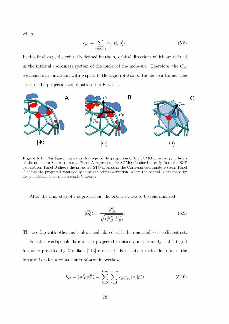
where
cpiπ =∑
j=x,y,z
cpij〈piπ|pij〉. (5.8)
In this final step, the orbital is defined by the pπ orbital directions which are defined
in the internal coordinate system of the nuclei of the molecule. Therefore, the Cpiπ
coefficients are invariant with respect to the rigid rotation of the nuclear frame. The
steps of the projection are illustrated in Fig. 5.1.
Figure 5.1: This figure illustrates the steps of the projection of the SOMO onto the pπ orbitalsof the minimum Slater basis set. Panel A represents the SOMO obtained directly from the SCFcalculation. Panel B shows the projected STO orbitals in the Cartesian coordinate system. PanelC shows the projected rotationally invariant orbital definition, where the orbital is expanded bythe pπ orbitals (shown on a single C atom).
After the final step of the projection, the orbitals have to be renormalised ,
|φND〉 =φ′ND√
〈φ′ND |φ′ND〉. (5.9)
The overlap with other molecules is calculated with the renormalised coefficient set.
For the overlap calculation, the projected orbitals and the analytical integral
formulae provided by Mulliken [113] are used. For a given molecular dimer, the
integral is calculated as a sum of atomic overlaps
Sab = 〈φND |φMA 〉 =atoms∑i∈D
atoms∑j∈A
cpiπcpjπ〈piπ|pjπ〉 (5.10)
78
To simplify the integrals, a local basis set is defined for each atom pair. The choice
of the local basis set is semi-trivial. One of the axes is the vector pointing from one
atom to the other (we chose this to be the z axis). The y axis is determined by an
arbitrary vector that is orthogonal to the z axis, and the x direction is constructed
as the cross product of the other axis vectors. The pπ orbitals of the atoms are
projected onto this local basis set
|piπ〉 = cx,i|pxloc〉+ cy,i|pyloc〉+ cz,i|pzloc〉. (5.11)
The overlap integrals for each atomic pair can be defined as the sum of pπ and pσ
overlaps at different nuclear separations R. The formulae also depend on the Slater
coefficients presented in Eq. (5.6) which differ for different quantum numbers and
elements [113]. The overlap is then
〈piπ|pjπ〉 = (c∗x,icx,j + c∗y,icy,j)Spπ(r, µip, µjp) + c∗z,icz,jSpσ(R, µip, µ
jp), (5.12)
where µip and µjp are the Slater decay coefficients of the p orbitals on atoms i and j
respectively.
It is easy to see that both the projection and the overlap calculation depend
on the Slater coefficients. There are many ways to calculate these coefficients for
different elements including the original method of Slater [117] and a more recent
approximation by Clementi et al. [118]. However since the basis set is small, µ was
kept as a parameter which was optimised to maximise the completeness ( Eq. (5.9))
of the projection and minimise the error in the electronic coupling calculation.
79

5.2 Training and test sets for the parameterisa-
tion of the overlap method
Firstly, to tackle the issue of the fitted parameters, a sufficiently broad set of
molecules had to be chosen. Since the HAB11 database [68] has been already tested
with various methods of coupling calculation it proved to be a good starting point.
It contains a variety of π-conjugated molecules to calibrate and test the Slater coef-
ficients µ and the conversion factor C.
The positively charged HAB11 set consists of a series of stacked π-conjugated sys-
tems which contain heteroatoms: oxygen, nitrogen, and sulphur. These molecules are
the building blocks of many semiconducting materials (e.g. thiophene for PBTTT
[19]), yet small enough for calculation of Hab at high levels of ab initio theory. Since
there were only a few data points that had SOMO contribution on the heteroatoms
these were omitted from the basis set. These molecules would have provided an insuf-
ficient basis set for calibrating the Slater coefficients for the heteroatoms. Therefore
the set was reduced to the seven molecules which had density on the carbon atoms
only. These were ethylene, cyclobutadiene, cyclopentadiene, benzene, pyrrole, furane
and thiophene. The configuration was the same for all seven molecules, π-stacking
with an enforced mirror plane between the monomers. The couplings were calculated
at different stacking distances given by 3.5, 4.0, 4.5 and 5.0 A. In the following, this
data set is referred to as HAB7.
The acenes data set was used to investigate the size dependence of the π-
conjugated system. A series of positively charged polyacenes were used increasing
in size from naphthalene to pentacene. The dimer structure was similar to the one
applied for the HAB7 set, π-stacked using the same stacking distances.
In order to test the effects of different configurations, a data set of fifteen ran-
domly oriented positively charged thiophene dimers was also analysed at different
80
distances. These configurations tested the effects of different intermolecular orienta-
tions.
As the analytic overlap method is less size-limited, larger molecules can also be
implemented in the test set. Since the focus in this piece of work is on organic semi-
conductors, fullerenes are used both for parameter calibration and testing. The set
termed C60 was created by choosing three rotationally different negatively charged
C60 dimers and calculating the coupling at seven different centre-to-centre distances
from 9 to 15 A (Fig. 5.2), creating a set of twenty-one dimers.
Another set of negatively charged C60 molecules consisted of twenty equidistant
rotationally different dimers chosen from the ∼ 27000 published in Ref [45]. The
separation of the dimers was set to 10.1 A. This data set is termed C60R.
A series of dimers from the monoclinic and triclinic PCBM structure were also
included for which the coupling values were calculated in the reduced state in an
earlier publication [5, 49]. PCBM is about the size limit of our chosen reference
method: FODFT. This data set is denoted as PCBM.
Another important aspect of these last three data sets is the curvature in the
molecular structure. Unlike the other test molecules, C60 and PCBM are not flat.
The radial component of the HOMO is not symmetric with respect to the surface
of the buckyball; the lobe outside the cage is slightly larger than the lobe inside the
cage. This implies a non-negligible contribution from the 2s orbital on each C atom
in addition to pπ.
So far all the data sets represented carbon systems. To expand the applicability
the four imidazole configurations from HAB11 and a set of five positively charged
stacked porphins were used to optimise the µp value for N.
Furthermore since the data set has been already tested with other methods in
Chapter 4 the HAB7- set, consisting of negatively charged anthracene, tetracene,
pentacene, perylene, perylene-diimide, perfluorinated anthracene, and prophin, is
also added to the test sets (See Fig. 4.2), along with the six randomly oriented
81

benzene
cyclobutadiene
cyclopentadiene
thiophenefurane
C60
ethylene
training set
imidazole
pyrrole
acenes
n
porphin
test set
PCBM
imidazole
n=0 naphthalene n=1 anthracenen=2 tetracenen=3 pentacene
Figure 5.2: The arene, acene and fullerene compounds that were included in our coupling referencecalculations. The blue frame marks the training set which was used to obtain the fitted parametersfor Eq. (5.1). The red frame marks the test set which were used independently to test the generalityof the fitted parameters. In addition, the HAB7- set shown in Fig. 4.2 and the randomly orientedanthracene molecules were also used as test sets.
negatively charged anthracene dimers from Chapter 4.
5.3 Computational details for reference coupling
calculations and fast overlap method
The reference calculations were done with fragment orbital density functional theory.
Although CDFT with 50% exact exchange gave the best results this is not feasible
for systems as large as a PCBM dimer.
The simulation details were analogous to the ones presented in Chapter 4 for the
82

HAB7, the acenes, the tiophenes, and the porphin set. The structures of the HAB7,
acenes, and thiophene datasets were taken from Ref. [68]. The C60, C60R, and the
PCBM sets were also calculated using the CPMD code with 4 A vacuum around
the isolated dimers but the pseudopotentials were Goedecker–Teter–Hutter (GTH)
type dispersion corrected atom centred pseudopotentials and Hockney type Poisson
solver permitting a smaller box size. The basis set cut-off was slightly increased to
90 Ry as the GTH pseudopotentials are somewhat harder than the TM potentials
used earlier. The convergence criterion for the Kohn–Sham orbitals was that the
maximum component of the energy gradient had to be lower than 8.5×10⁻⁷ a.u. in
order to converge the orbitals. The structures were taken from Ref [45] and Ref [49].
The FODFT coupling values were scaled by a factor of 1.3. This correction factor
was obtained by comparing the FODFT values to MRCI+Q and NEVPT2 results
for oxidised dimers [68], and similar correction factor was derived in the reduced
state in Chapter 4. The corrected set is referred to as sFODFT. To make sure that
the states were coupled consistently between the different methods, the NEVPT2
spin densities and the FODFT spin densities were compared by visual observation.
Before calculating the reference values, the available accuracy of the FODFT
calculations were tested. While the numerical accuracy in the low coupling regime
is not an issue for small molecules, where the coupling is in the order of several
hundred meV, it becomes more important when C60 and PCBM is assessed. For
the fullerene molecules the coupling values are lower and strongly depend on the
relative orientation of the dimers [45]. The FODFT coupling accuracy is limited
by the finite integration grid and the basis set cut-off. Testing several C60 dimers,
the effect of rotating the entire dimer in the box resulted in a fluctuation in the
coupling value of maximum 0.2 meV. This can be reduced by increasing the real
space grid of the calculation. However, this increases the computational costs for
larger box sizes significantly. Therefore, any data point below 0.2 meV was omitted.
The problem likely arises from the pseudopotentials which are generated by creating
83
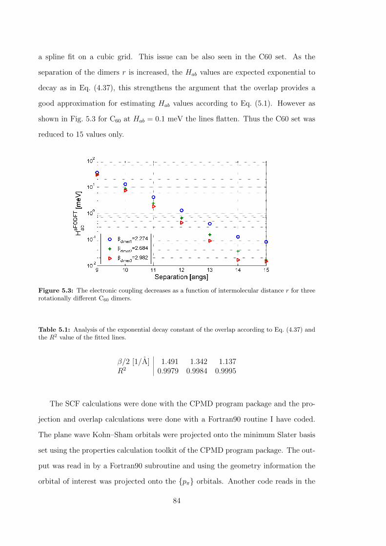
a spline fit on a cubic grid. This issue can be also seen in the C60 set. As the
separation of the dimers r is increased, the Hab values are expected exponential to
decay as in Eq. (4.37), this strengthens the argument that the overlap provides a
good approximation for estimating Hab values according to Eq. (5.1). However as
shown in Fig. 5.3 for C60 at Hab = 0.1 meV the lines flatten. Thus the C60 set was
reduced to 15 values only.
Figure 5.3: The electronic coupling decreases as a function of intermolecular distance r for threerotationally different C60 dimers.
Table 5.1: Analysis of the exponential decay constant of the overlap according to Eq. (4.37) andthe R2 value of the fitted lines.
β/2 [1/A] 1.491 1.342 1.137R2 0.9979 0.9984 0.9995
The SCF calculations were done with the CPMD program package and the pro-
jection and overlap calculations were done with a Fortran90 routine I have coded.
The plane wave Kohn–Sham orbitals were projected onto the minimum Slater basis
set using the properties calculation toolkit of the CPMD program package. The out-
put was read in by a Fortran90 subroutine and using the geometry information the
orbital of interest was projected onto the pπ orbitals. Another code reads in the
84

set of coefficients and the nuclear configuration. The orbitals are reconstructed on
the nuclear frame and the Slater integrals are calculated as explained in Section 5.1.
Due to their degenerate SOMOs, benzene and the fullerene derivatives needed
extra attention when doing the coupling calculation. The SOMO of C−60 is identical
to the LUMO of the neutral C60, the orbital is three-fold degenerate and belongs to
the T1u irreducible representation of the Ih point group [119]. The excess charge does
not break the symmetry significantly. In the Kohn–Sham calculations, the three-fold
degeneracy for C60 and the 2-fold degeneracy for benzene is preserved to the accu-
racy of 10 meV. Although the electronic structure of PCBM− is similar to that of
C60 the orbitals are slightly perturbed by the side chain, resulting in partially lifted
degeneracy. The SOMO-LUMO separation is 40 meV and the LUMO LUMO+1
separation is larger than 100 meV. Therefore at room temperature PCBM is only
2-fold degenerate. The orbital coupling was consistent in the benzene, the PCBM−
and the C−60 cases. During the initialisation step, CPMD consistently localised the
excess electron on the first atom in the code which resulted in the HOMO always
having the same relative orientation compared to the atomic indices. Most impor-
tantly, the SOMO co-rotated with nuclear frame. This means that one set of orbital
coefficients obtained for an isolated C60 or PCBM molecule was sufficient to describe
all dimer configurations of those molecules.
5.4 Results and discussion
This section discusses the generality, accuracy and speed of the overlap method. In
the first half, the test set is used to determine whether only one C parameter can
be used to determine the Hab for different molecules with Eq. (5.1) or not. In the
second half, the focus is on the possible reduction of the basis set to a smaller one
consisting of the pπ orbitals only and on the accuracy which can be achieved with
85
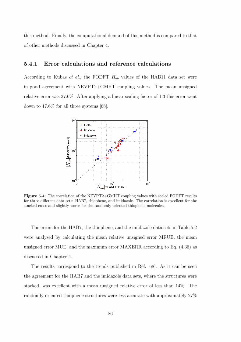
this method. Finally, the computational demand of this method is compared to that
of other methods discussed in Chapter 4.
5.4.1 Error calculations and reference calculations
According to Kubas et al., the FODFT Hab values of the HAB11 data set were
in good agreement with NEVPT2+GMHT coupling values. The mean unsigned
relative error was 37.6%. After applying a linear scaling factor of 1.3 this error went
down to 17.6% for all three systems [68].
Figure 5.4: The correlation of the NEVPT2+GMHT coupling values with scaled FODFT resultsfor three different data sets: HAB7, thiophene, and imidazole. The correlation is excellent for thestacked cases and slightly worse for the randomly oriented thiophene molecules.
The errors for the HAB7, the thiophene, and the imidazole data sets in Table 5.2
were analysed by calculating the mean relative unsigned error MRUE, the mean
unsigned error MUE, and the maximum error MAXERR according to Eq. (4.36) as
discussed in Chapter 4.
The results correspond to the trends published in Ref. [68]. As it can be seen
the agreement for the HAB7 and the imidazole data sets, where the structures were
stacked, was excellent with a mean unsigned relative error of less than 14%. The
randomly oriented thiophene structures were less accurate with approximately 27%
86

Table 5.2: Correlation of the GMHT+NEVPT2 and sFODFT coupling values for HAB7, thio-phene, and imidazole. MRUE, MUE, and MAXERR values were calculated according to Eq. (4.36).
set MRUE [%] MUE [meV] MAXERR [meV]HAB7 13.7 15.7 35.8thiophene 26.6 48.2 94.4imidazole 12.9 12.7 15.6
relative error (Fig. 5.4). Since the scaling factor 1.3 always decreased the error,
sFODFT values were used as reference Hab values.
5.4.2 Overlap method with DFT orbitals
The next step was to test the validity of Eq. (5.1) on the training and test systems.
At first, the coupling values are compared to the real space integrals of the SOMO
orbitals obtained by DFT using the full plane wave orbitals without any reduction of
the basis set. Then, the proportionality between couplings calculated with FODFT
and the projected minimum STO orbitals is discussed. Finally the two overlap
values calculated with plane wave DFT orbitals and with projected STO orbitals are
compared.
Since the calculated Hab values cover several orders of magnitude ranging from 0.2
to 1000 meV, to represent the entire range the C60 and HAB7 sets were combined
into a training set to fit the conversion factor C. It is expected that the MRUE
would underestimate the error for small couplings. Therefore, in order to have a
fairer assessment for the broad range the root-mean-square error of the logarithm
was minimised as
ERMSLE = exp
√√√√ 1
N
N∑i=1
(ln
∣∣∣∣ Hrefab
Hcalcab
∣∣∣∣)2
i
(5.13)
where Hrefab is the sFODFT coupling value and Hcalc
ab was calculated as Hcalcab = CSab.
87

The maximum error was defined as
MAXUL = exp
(max
(ln
∣∣∣∣ Hrefab
Hcalcab
∣∣∣∣)) . (5.14)
The optimimum linear scaling factor obtained by minimising Eq. (5.13) was C =
Table 5.3: Errors of the calculated Hab values using Eq. (5.1) with full SCF basis set compared tothe sFODFT Hab values. ERMSLE values give a rough estimate of the factor of the error thereforethere are no units presented.
set ERMSLE MAXULtraining set 1.6 3.7
acenes 1.5 1.9thiophene 1.7 2.5
C60R 1.8 8.2PCBM 1.8 3.9porphin 1.8 2.7
imidazole 1.4 1.7HAB7- 1.5 2.7
anthracene 2.3 4.3
3.498 eV. The correlation was very good in the higher coupling regime but the errors
became somewhat larger at the sub-meV level. However, it can be seen in Fig. 5.5
that despite the wide variety of molecules and the different errors, the different
compounds matched the same line.
5.4.3 Projection on the STO basis set
The main question discussed in this section is whether the good correlation between
the coupling and the overlap can be retained when the overlap Sab calculated with
the DFT orbitals is replaced by the overlap between the projected orbitals, Sab as in
Eq. (5.10).
Using the minimum STO basis set introduces data loss, therefore the effect on
the orbital had to be assessed. In order to maximise the completeness of the pro-
jection, the Slater coefficient that described the 2p orbital of carbon µC2p in the
88

Figure 5.5: The correlation of the full SCF SOMO orbital overlaps with the scaled sFODFTcoupling values. Using a different error definition to fit the line such as MURE would have resultedin a steeper line as the higher coupling values would have been included with a more significantweight.
CPMD code was optimised. In the original version of the code, µC2p = 1.5679 bohr−1
was used which was calculated using the effective nuclear charges by Clementi
[118]. However, for C60 the Slater coefficient that maximised the completeness was
µC2p = 1.3125 bohr−1. This value produced more completeness for the molecules of
the HAB7 set, though the µC2p dependence was much weaker in this case [Table 5.4].
A similar analysis was performed for the nitrogen: the optimum Slater coefficient
value was µN2p = 1.7 bohr−1. The effect of a larger Slater basis set on the complete-
Table 5.4: Different µC2p values for the projection give different completeness (See Eq. (5.9)).
The completeness of the monomers of the HAB7 set were averaged. The HAB7 set was not verysensitive tox changes in the Slater coefficient, but the C60 set had stronger µ dependency.
µCp [bohr−1] 1.0 1.1 1.2 1.3 1.4 1.5 1.6
||φ′N || C60 0.939 0.960 0.972 0.977 0.975 0.967 0.956
||φ′N || HAB7 - - - 0.978 - - 0.975
ness was also tested. For this, the 3s, 3p and 4s, 4p basis functions were added
89
to the minimum Slater basis set. The coefficients for carbon on these additional
basis functions were in general two orders of magnitude smaller than the 2s, 2p
coefficients, and the completeness did not change significantly.
Secondly, the effect of further projection to the pπ basis set had to be de-
termined. For the HAB7, acenes, imidazole and porphin data sets, the projected
coefficients on the s orbitals and on the p orbitals perpendicular to the pπ-direction
were < 0.001. However, both PCBM and C60 had some densities on the s orbitals,
although even the largest s coefficient (0.015) was an order of magnitude smaller
than the largest p coefficient (0.280). To test the effect of the s orbitals on the norm
calculation, the basis set was increased to s, pπ. In this case, the projected orbital
in Eq. (5.7) took the form of
|φ′ND〉 ≈ |φND〉 =N∑i
csi |si〉+ cpiπ |piπ〉. (5.15)
The overlap instead of Eq. (5.10) was calculated as
Sab =atoms∑i∈D
atoms∑j∈A
c∗sicsj〈si|sj〉+ c∗piπcpjπ〈piπ|pjπ〉+ c∗piπcsj〈p
iπ|sj〉+ c∗sicpjπ〈s
i|pjπ〉, (5.16)
where the integrals in Eq. (5.12) became
〈piπ|pjπ〉 = (c∗x,icx,j + c∗y,icy,j)Spπ(R, µip, µjp) + c∗z,icz,jSpσ(R, µip, µ
jp), (5.17a)
〈piπ|sj〉 = c∗z,iSpσ−s(R, µip, µ
js), (5.17b)
〈si|pjπ〉 = cz,jSs−pσ(R, µis, µjp), (5.17c)
〈si|sj〉 = Ss−s(R, µis, µ
js). (5.17d)
As shown in Table 5.5, adding the s orbitals only changed the completeness slightly.
90

Table 5.5: Orbital norms calculated with the analytic overlap program using SCF orbitals pro-jected on the minimum STO basis set. The calculations marked with s included the s orbitals toowhile the unmarked overlap values only contain the pπ orbitals orthogonal to the plane of conju-
gation. 〈||φ′N
D ||〉 refers to the mean of the norm while σ(||φ′
N
D ||)
is the standard deviation. The
molecules of the HAB7 and acenes data set were unaffected by the inclusion as the s coefficientswere 0.
set 〈||φ′ND ||〉 σ(||φ′ND ||
)HAB7 0.988 0.0025acenes 0.991 0.0004
C60, PCBM 0.987 0.0224Cs
60, PCBMs 0.991 0.0224
5.4.4 Overlap method with the STO basis set
As was shown in the previous section, a very good completeness can be achieved
with the STO basis set. However, the question is how this affects the overlap. It
is easy to see that a Slater coefficient which gives good completeness might capture
well the electronic structure closer to the nuclei, but that part of the orbital has
little effect on the overlap, unlike the exponential tail of the STO basis functions.
The aim was to derive a correlation plot similar to Fig. 5.5 between the electronic
couplings calculated with FODFT and the analytical overlap integrals calculated
with the minimum STO basis set. The same training set was used for this fit and
similarly the ERMSLE of the logarithm was minimised (See Eq. (5.13)), however in
this case the Slater coefficient was optimised as well to improve the fit.
Hab = CSab(µ) (5.18)
where Sab is the overlap calculated with the SOMO orbitals expanded in the pπ ba-
sis set (See Eq. (5.10)). The best fit was µC2p = 1.0 bohr−1 with the conversion factor
C = 1.819 eV (Table 5.6). This Slater coefficient is much smaller than the afore-
mentioned Clementi–Raimondi value of 1.5679 bohr−1 It is worth noting that the
C parameter is very sensitive to the small changes in µ. This is the reason why the
91

optimum C value is much smaller than other published values [48, 111]. The reason
behind the small decay coefficient could be that at our typical interatomic distances
(3 to 8 A) this decay coefficient represents the orbital shape better.
Table 5.6: Different µC2p values around the best fitted µC
2p and the conversion factor C whichapproximates best the sFODFT coupling values according to Eq. (5.18). Relative and logarithmicerrors calculated according to Eq. (4.36) and Eq. (5.13) respectively.
µCp [bohr−1] ERMSLE MRUE [%] C [meV] R2
0.90 1.58 39 1095 0.970.95 1.48 32 1418 0.981.00 1.45 30 1819 0.981.10 1.63 91 3295 0.97
Including the s orbital in the SOMO of C60 had a negligible effect on the accuracy
of the integral (Table 5.7).
Table 5.7: Different µC2s values and the corresponding ERMSLE values on the training set com-
paring approximate coupling values calculated with Eq. (5.18) to sFODFT reference values. Theeffect of the s orbitals is much smaller compared to the p orbitals. The value of the conversionfactor was not affected by the larger basis set. All values are in bohr−1.
µCp
µCs 0.90 1.00 1.10 1.70
1.0 1.45 1.43 1.45 1.45
The Slater coefficient µN2p was optimised using the porphin and imidazole sets.
The ERMSLE was minimised by varying the µN2p value, keeping the conversion factor
as 1819 meV. The optimisation resulted in µN2p = 1.5 bohr−1.
The analytical coupling values for all the other sets were calculated with these
µ and C parameters as shown in Fig. 5.6 and a similar error analysis to the one in
section 5.4.2 was performed in Table 5.8.
Using µCp =1.0 bohr−1, the analytically calculated Sab values were plotted against
the full real space plane wave integral Sab values. One can clearly see the effect of
the reduced Slater coefficient in Fig. 5.7: the slope on the logarithmic plot is roughly
0.76. This value corresponds well to the ratio between the Slater coefficient used for
92

Figure 5.6: The correlation of analytically calculated orbital overlaps using the pπ orbitals fromthe minimum STO basis set with the scaled sFODFT coupling values.
Table 5.8: The errors of the analytically calculated Hab values compared to the sFODFT Hab
values. ERMSLE and MAXUL values give a rough estimate of the factor of the error thereforethese values are unitless and were calculated according to Eq. (5.13) and Eq. (5.14).
set ERMSLE MAXULtraining set 1.4 2.9
acenes 1.3 1.6thiophene 1.5 2.8
C60R 2.7 15.7PCBM 1.8 3.0porphin 1.9 2.6
imidazole 1.4 1.5HAB7- 1.5 1.9
anthracene 2.2 5.1
the overlap calculation (1.000 bohr−1) and the Slater coefficient used for the orbital
projection (1.3125 bohr−1). It is important to point out that the thiophene and the
randomly oriented C60R set matches the fitted line better on the Sab vs. Sab plot
93
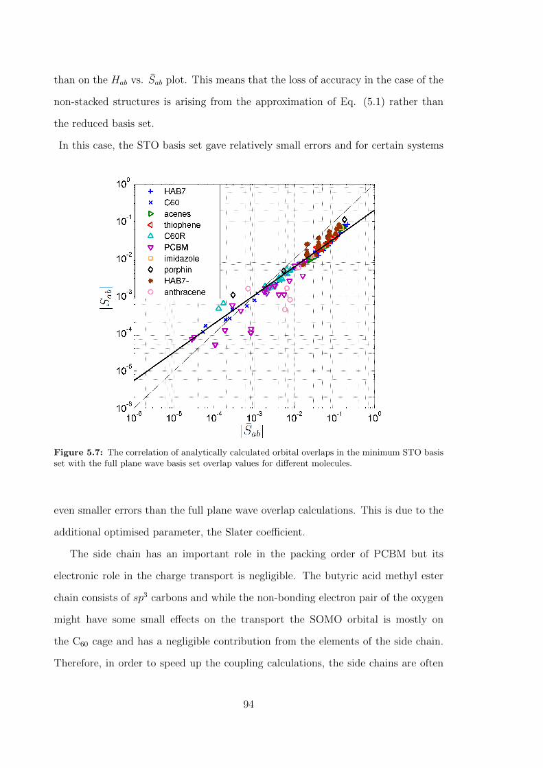
than on the Hab vs. Sab plot. This means that the loss of accuracy in the case of the
non-stacked structures is arising from the approximation of Eq. (5.1) rather than
the reduced basis set.
In this case, the STO basis set gave relatively small errors and for certain systems
Figure 5.7: The correlation of analytically calculated orbital overlaps in the minimum STO basisset with the full plane wave basis set overlap values for different molecules.
even smaller errors than the full plane wave overlap calculations. This is due to the
additional optimised parameter, the Slater coefficient.
The side chain has an important role in the packing order of PCBM but its
electronic role in the charge transport is negligible. The butyric acid methyl ester
chain consists of sp3 carbons and while the non-bonding electron pair of the oxygen
might have some small effects on the transport the SOMO orbital is mostly on
the C60 cage and has a negligible contribution from the elements of the side chain.
Therefore, in order to speed up the coupling calculations, the side chains are often
94
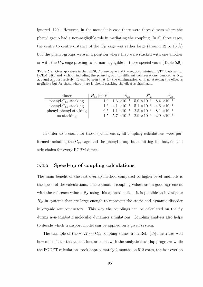
ignored [120]. However, in the monoclinic case there were three dimers where the
phenyl group had a non-negligible role in mediating the coupling. In all three cases,
the centre to centre distance of the C60 cage was rather large (around 12 to 13 A)
but the phenyl-groups were in a position where they were stacked with one another
or with the C60 cage proving to be non-negligible in those special cases (Table 5.9).
Table 5.9: Overlap values in the full SCF plane wave and the reduced minimum STO basis set forPCBM with and without including the phenyl group for different configurations, denoted as Sab,Sab and S′ab respectively. It can be seen that for the configuration with no stacking the effect isnegligible but for those where there is phenyl stacking the effect is significant.
dimer Hab [meV] Sab S ′ab Sabphenyl-C60 stacking 1.0 1.3 ×10⁻⁴ 5.0 ×10⁻⁵ 8.4 ×10⁻⁴
phenyl-C60 stacking 1.6 4.1 ×10⁻⁴ 5.1 ×10⁻⁵ 4.6 ×10⁻⁴
phenyl-phenyl stacking 0.5 1.1 ×10⁻⁴ 2.5 ×10⁻⁵ 8.1 ×10⁻⁴
no stacking 1.5 5.7 ×10⁻⁴ 2.9 ×10⁻⁴ 2.9 ×10⁻⁴
In order to account for those special cases, all coupling calculations were per-
formed including the C60 cage and the phenyl group but omitting the butyric acid
side chains for every PCBM dimer.
5.4.5 Speed-up of coupling calculations
The main benefit of the fast overlap method compared to higher level methods is
the speed of the calculations. The estimated coupling values are in good agreement
with the reference values. By using this approximation, it is possible to investigate
Hab in systems that are large enough to represent the static and dynamic disorder
in organic semiconductors. This way the couplings can be calculated on the fly
during non-adiabatic molecular dynamics simulations. Coupling analysis also helps
to decide which transport model can be applied on a given system.
The example of the ∼ 27000 C60 coupling values from Ref. [45] illustrates well
how much faster the calculations are done with the analytical overlap program: while
the FODFT calculations took approximately 2 months on 512 cores, the fast overlap
95

program calculates these values in 87 seconds on a single node. This is excluding
the SCF step calculating and projecting the SOMO orbital on a single minimised
C60 molecule which takes 20 minutes on 512 cores. As expected, the fast overlap
method scales better with time than any other method discussed in Chapter 4 as
can be seen in Fig. 5.8.
Figure 5.8: CPU time of different coupling calculation methods for different molecules and theerror compared to the GMHT with SCS-CC2 reference values. The colour coded stems refer to themean unsigned relative error Eq. (4.36); the solid stems show the scaled errors using the uniformscaling factors from Table 4.2; while the dashed stems show the actual relative error of differentmethods. The analytic overlap method is abbreviated as AOM on this plot.
It is worth mentioning that the comparison was done for the pπ-only overlap
calculations. While s orbitals had non-zero contribution to the SOMO of C60 and
PCBM sets their effect on the overlap was negligible. However, as the complexity of
the formulae increased a significant overhead appeared in the calculation increasing
the calculation of the coupling for a single C60 dimer from 0.003 s to 0.03 s.
96

5.4.6 Conclusions of the overlap method
It was demonstrated in this section that the linear relation of Eq (5.1) gives a good
approximation to electronic coupling matrix elements between π-conjugated organic
molecules in the range relevant to electron transport in the condensed phase (5 to
500 meV). A linear relation has been derived for single donor-acceptor pairs before,
but here it is shown that a very diverse set of donor-acceptor pairs including stacked
acenes, arenes with S, N, and O heteroatoms, and buckyballs can be described with a
single proportionality constant. Most importantly, this linear correlation is retained
or can be even improved if the overlap is calculated in terms of a minimum STO
basis set with optimised Slater decay coefficients. Gaussian type orbitals would have
been alternative method to use the analytic overlap method however using minimum
STO basis set in combination with the projection to the pπ orbitals saves memory by
using a single basis function per atom. While the integral formula is in general more
complicated for slater type orbitals then it is for GTO the atoms which contribute the
most to the couplings are mostly C atoms and for the same atom type the analytic
integral formula is considerably simple [113].
This also provides a tool to estimate electronic couplings analytically, leading to
speed-ups of around 6 orders of magnitude compared to standard DFT calculations
for molecules typically used in molecular OSCs. Together with a fast estimator for
site energies using for example polarisable or non-polarisable force fields, this scheme
provides the basis for a fast yet reasonably accurate estimation of the electronic
Hamiltonian that can be used in NAMD simulations of charge transport in OSC
materials.
97

5.5 Analysis of heme systems with the overlap
method
An extensive study was presented on the analytic overlap method in the previous
section but the influence of thermal fluctuations on electronic couplings was not dis-
cussed. As the method is only fast if we have a set of coefficients obtained from
SCF calculation, this can be an issue when the AOM is used in molecular dynamics
simulations. Since during MD the molecules are not rigid, obtaining a set of coeffi-
cients for every molecule in every snapshot could introduce a significant overhead. In
this section, the effects of thermal fluctuations on Hab are discussed on various heme
systems. An idealised set of coefficients were obtained from the minimised structure
and were tested against FODFT results using the AOM on a molecular dynamics
trajectory of three different heme systems.
5.5.1 Structures
Molecular dynamics trajectories of two deca-heme systems extracted from multi-
heme cytochromes MtrC and its homologue MtrF were used for these calculations.
MtrC can be found in the outer membrane of Schewanella oneidensis. S. oneidensis
is an example of a dissimilatory metal reducing bacteria: in anaerobic environments
they use extracellular insoluble transition metal oxides as terminal electron acceptors
in their respiratory chain, such as manganese oxide [79]. Finally, the small tetra-
heme cytochrome STC is investigated, which also functions as ET protein in S.
oneidensis [121]. The three heme systems can be seen in Fig. 5.9.
Structures for MtrF, MtrC and STC were taken from molecular dynamics tra-
jectories reported in Refs. [79], [80] and [122], respectively.
From each trajectory, 25 snapshots were extracted, separated by 1 ns. The hemes
were extracted according to the methodology discussed in Ref. [79] including the axial
98

Figure 5.9: Multi-heme systems extracted from MtrF (Panel A), MtrC (Panel B), and STC(Panel C) protein SCF minimisation of the protein structure deposited in the data base. Theenvironment of the multi-heme structure is not visible on the panel and did not participate inthe electron structure calculations but was involved in the molecular dynamic simulation. Themolecular dynamics calculations were done on the entire protein structure in water. For the couplingcalculations the prophirin rings were extracted from these trajectories as in [79]. The blue circledenotes a stacked dimer structure. The red circle shows a T-shaped structure and the green circleis around a coplanar structure.
histidines but excluding all substituents of the porphin ring. The dimer structures
were analysed according to stacking structure, Fe-to-Fe interatomic distance, and
edge-to-edge distance. The edge-to-edge distance was calculated by identifying the
nearest π-conjugated carbon atoms of the two porphin rings. For the MtrF and the
MtrC, eight heme pairs were identified for both structures for which the couplings
were expected to be non-negligible. For the STC structure, three such pairs were
found.
Three types of stacking are distinguished for these dimers: stacked, T-shaped,
and coplanar. The type of stacking is in most cases reflected in the Fe-to-Fe and
edge-to-edge distance ranges as can be seen in Table 5.10.
99

Table 5.10: Average Fe-to-Fe and edge-to-edge distance of the different types of heme dimers.The edge-to-edge distance was calculated using the smallest distance between the carbon atoms ofthe porphyrin rings. The numbers in the brackets show the maximum deviation from the averagevalues for each stacking type.
stacked T-shaped coplanar
dedge−edge [A] 4.44(±1.4) 5.85(±0.56) 6.62(±1.45)
dFe−Fe [A] 10.49(±1.65) 11.76(±0.86) 13.75(±1.25)
5.5.2 Simulation details
Similarly to the previous section, the reference calculations were done with FODFT.
The FODFT results for MtrF were taken from the publication Ref. [79]. The FODFT
calculations for MtrC and STC were done analogously to Ref. [79], using PBE func-
tional with a 130 Ry basis set cut-off and GTH type pseudopotential replacing the
core electrons. The convergence criterion for the electronic gradient was 1×10⁻⁶ a.u.
The box size for the isolated system calculations was identified by centring every
dimer in the minimal possible box with a minimum of 4 A of vacuum between the
box wall and the outermost atoms of the molecules, and the longest minimal dimen-
sions were chosen. Therefore, all calculations were done in the same box size with
at least 4 A of vacuum around the molecules. Thus, the MtrC FODFT calculations
were done in a 32.2A× 20.7A× 20.5A orthorhombic box and the STC box size was
32.3A× 20.5A× 20.5A, also orthorhombic. All FODFT coupling values were multi-
plied with a ccorr polarisation correction factor, 1.7, derived in Ref. [79]; these results
are referred to as cFODFT.
The convergence of the coupling matrix elements with respect to the reciprocal
space plane wave cut-off (which is the basis set in plane wave calculations) was inves-
tigated for two configurations of a heme pair of MtrC. The results are summarised
in Table 5.11. At 110 Ry, the absolute error for the smallest and largest Hab were
0.1 and 0.3 meV respectively, relative to 130 Ry.
Analytic overlap method coupling results for porphin were discussed in the pre-
100

Table 5.11: cFODFT coupling values as a function of the plane wave basis set for assessing anoptimal and sufficient basis set. Both couplings are from MtrC. Structure A is a coplanar dimerand structure B is a stacked dimer.
basis set cut-off [Ry] Hab A [meV] Hab B [meV]150 0.10 2.12130 0.11 2.03110 0.24 2.32100 0.27 2.6490 0.55 2.7780 1.30 3.8770 1.68 4.09
Figure 5.10: The SOMO and SOMO-1 orbitals on the perfect heme. They were identified by theorientation of the d orbital: the SOMO and the SOMO-1 always contain dxz and dyz where thedirection z is along the axis formed by the histidine molecules.
vious section, but the heme molecules contain an iron core. In fact, the SOMO of
the heme has a significant lobe on the Fe atom. If the SOMO is projected on the
minimum STO basis set the completeness is 0.89, which is smaller than in the por-
phin case where the completeness was 0.96. If the Fe atom is omitted the projection
results in a 0.3 completeness. Omitting the contribution of the Fe atom, the orbitals
obtained for the AOM were normalised to ||φN ||2 = 0.3. The Slater coefficients were
µC2p = 1.0 bohr−1 and µN2p = 1.5 bohr−1. The contribution from the s orbitals were
negligible and, therefore omitted. The orbital expansion coefficients are obtained
101

from the SCF minimised idealised heme structure shown in Figure 5.10.
The expansion Eq. (5.4) can be generalised to include d orbitals, however this
could result in a loss of computational speed while the precision may not be improved
significantly. In this section, the analytic overlap method is tested against FODFT
values for the three proteins, where the contribution of the d orbitals is omitted.
This was motivated by the fact that in these systems the smallest Fe-to-Fe distance
is larger than 9.4 A and the 3d Clementi–Raimondi coefficient is 3.7 bohr−1 for Fe.
This is more than twice as much as the C 2p coefficient by Clementi [118]. Therefore,
the overlap of the Fe-d orbitals of one porphyrine molecule with any atom of the other
porphyrine is expected to be negligibly small.
Another issue arises from the degeneracy of the hemes. Fig. 5.10 depicts the
SCF minimised heme molecules and the two-fold degenerate SOMO and SOMO-1.
During the calculations, the orbitals were identified by the contribution on the dxz
and dyz orbitals where the z direction was along the axis determined by the histidine
molecules. However, during the MD the nuclear frame distorts and the degenerate
orbitals mix. Degenerate systems were presented in the previous section as well: for
benzene and C60 one orbital was chosen and was consistently used in the calculations.
In this case, the degeneracy cannot be circumvented as during molecular dynamics
each state is equally likely to be occupied and the states can mix due to dynamic
effects.
In order to overcome this issue, instead of comparing the couplings individually
like in the case of benzene and C60, the root-mean-square averages are compared.
According to Newton [123], if the coupling is not too strong an effective coupling
can be defined using the root-mean-square average of the possible coupling values.
RMS(Hab) =1√Nφ
√ ∑i,j∈φ
H2ij; φ = SOMO, SOMO− 1. (5.19)
All four possible coupling values are calculated for every snapshot of every dimer
102

with cFODFT and same is done with AOM couplings. Then, the four coupling
values are root-mean-square averaged according to Eq. (5.19) for both methods.
These averaged Hab and Sab values are compared.
The degeneracy also affects the accuracy of the cFODFT calculations. The maxi-
mum fluctuation for the same configuration was found to be 0.5 meV in the coupling
depending on the diagonalisation method when the Kohn–Sham energies were cal-
culated according to Lanczos or Davidson and based on the initial state. This is
possibly due to the slight fluctuations in how the SOMO and SOMO-1 mixes for
heme dimers.
5.5.3 Results and discussion
Fig 5.11 depicts the correlation between the analytic overlap and the FODFT cou-
pling values. For all three proteins the RMS(Hab) and RMS(Sab) showed a much
wider spread than for the systems presented in Section 5.1. The three types of stack-
ings are clearly distinguishable with the exception of one T-shaped heme pair in the
STC system which showed high couplings, both with the AOM and the FODFT
method, resulting in coupling and overlap values which are closer to the lower end of
the stacked values. It can be seen that most of the coplanar values were below the
accuracy of the cFODFT method, here the correlation curve flattens. On the other
hand, it seems that there is a large spread even for values above 0.5 meV. This is
particularly prominent for the stacked values where similar overlap values seem to
expand over two orders of magnitude.
On panel B, of Fig. 5.11, the three different systems can be seen: STC showed
the largest coupling values while MtrF and MtrC showed similar coupling ranges
(MtrC having higher values than MtrF with cFODFT but similar overlap values
with AOM). The fitting method to derive a proportionality constant was the same as
in Section 5.1 by minimising the ERMSLE according to Eq. (5.13). The results can
be seen in Table 5.12 for the different heme systems and in Table 5.13 for all systems.
103

Figure 5.11: On panel A, the correlation between electronic coupling and analytic overlap valuescan be seen for the three different stacking types for MtrF, MtrC , and STC. On panel B, thesame correlation can be seen for the three different multi-heme systems. The black line depicts thebest fit. The red line marks the accuracy of the cFODFT results (0.5 meV). There is a significantvariation in the coupling values even within the different stacking types.
Table 5.12: Proportionality constants for different cFODFT coupling and AOM overlap correla-tions for the different stacking types on their own and combined with other stacking types.
MtrF MtrC STCC [meV] ERMSLE C [meV] ERMSLE C [meV] ERMSLE
stacked 2760 1.83 6308 1.80 1327 1.41stacked+T 3252 2.06 7801 2.06 3019 2.67all 3870 1.75 8152 2.15 3019 2.67
The constant of proportion C varies a lot for the heme systems depending on the
geometry of the dimers, which makes it more difficult to find a single conversion factor
to describe all dimers. The fitted values correspond to our observation: the smaller
the couplings, the more likely that the analytic overlap method underestimates the
values. As a consequence, if the smaller coupling values are included in the fit
the correlation coefficient C becomes larger. It is interesting to note that for the
STC stacked system where the couplings were the largest, the correlation coefficient
104
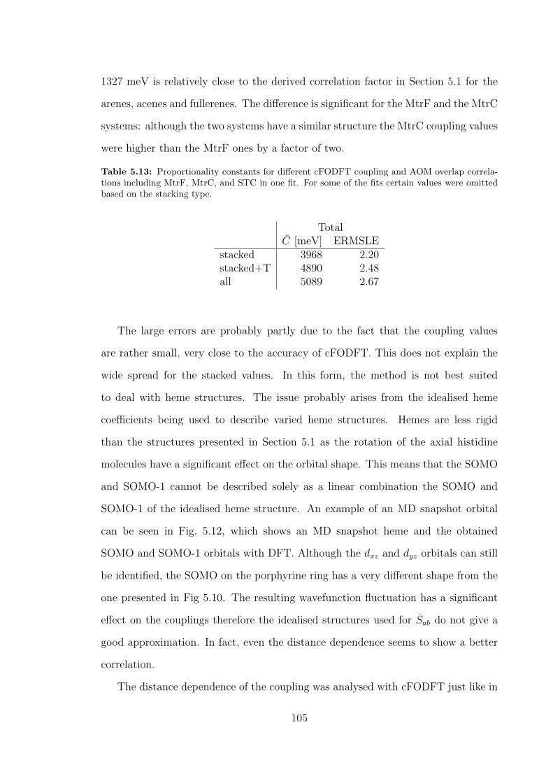
1327 meV is relatively close to the derived correlation factor in Section 5.1 for the
arenes, acenes and fullerenes. The difference is significant for the MtrF and the MtrC
systems: although the two systems have a similar structure the MtrC coupling values
were higher than the MtrF ones by a factor of two.
Table 5.13: Proportionality constants for different cFODFT coupling and AOM overlap correla-tions including MtrF, MtrC, and STC in one fit. For some of the fits certain values were omittedbased on the stacking type.
TotalC [meV] ERMSLE
stacked 3968 2.20stacked+T 4890 2.48all 5089 2.67
The large errors are probably partly due to the fact that the coupling values
are rather small, very close to the accuracy of cFODFT. This does not explain the
wide spread for the stacked values. In this form, the method is not best suited
to deal with heme structures. The issue probably arises from the idealised heme
coefficients being used to describe varied heme structures. Hemes are less rigid
than the structures presented in Section 5.1 as the rotation of the axial histidine
molecules have a significant effect on the orbital shape. This means that the SOMO
and SOMO-1 cannot be described solely as a linear combination the SOMO and
SOMO-1 of the idealised heme structure. An example of an MD snapshot orbital
can be seen in Fig. 5.12, which shows an MD snapshot heme and the obtained
SOMO and SOMO-1 orbitals with DFT. Although the dxz and dyz orbitals can still
be identified, the SOMO on the porphyrine ring has a very different shape from the
one presented in Fig 5.10. The resulting wavefunction fluctuation has a significant
effect on the couplings therefore the idealised structures used for Sab do not give a
good approximation. In fact, even the distance dependence seems to show a better
correlation.
The distance dependence of the coupling was analysed with cFODFT just like in
105
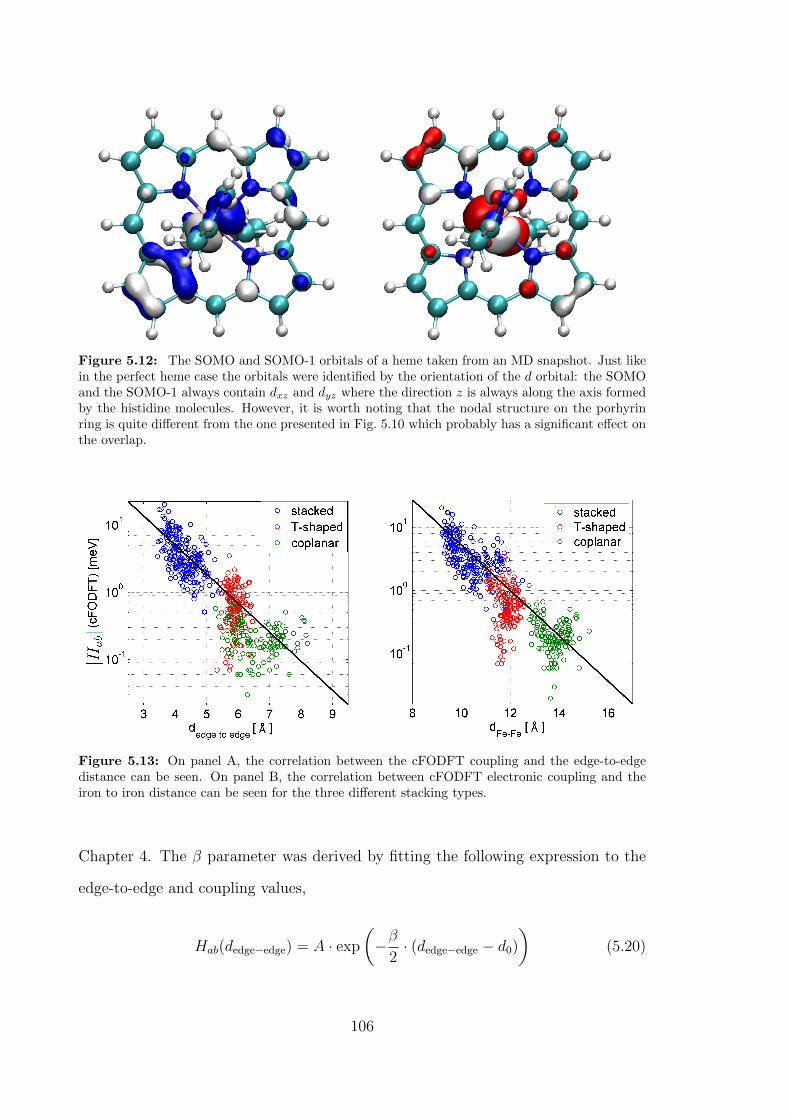
Figure 5.12: The SOMO and SOMO-1 orbitals of a heme taken from an MD snapshot. Just likein the perfect heme case the orbitals were identified by the orientation of the d orbital: the SOMOand the SOMO-1 always contain dxz and dyz where the direction z is always along the axis formedby the histidine molecules. However, it is worth noting that the nodal structure on the porhyrinring is quite different from the one presented in Fig. 5.10 which probably has a significant effect onthe overlap.
Figure 5.13: On panel A, the correlation between the cFODFT coupling and the edge-to-edgedistance can be seen. On panel B, the correlation between cFODFT electronic coupling and theiron to iron distance can be seen for the three different stacking types.
Chapter 4. The β parameter was derived by fitting the following expression to the
edge-to-edge and coupling values,
Hab(dedge−edge) = A · exp
(−β
2· (dedge−edge − d0)
)(5.20)
106
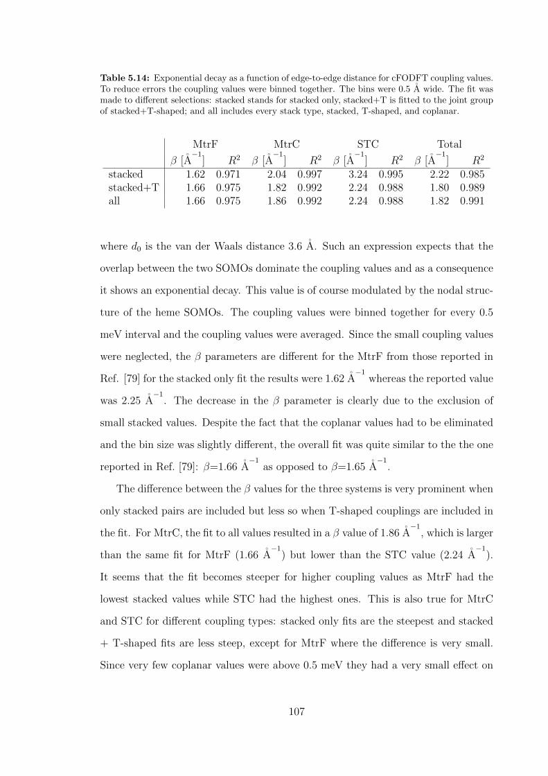
Table 5.14: Exponential decay as a function of edge-to-edge distance for cFODFT coupling values.To reduce errors the coupling values were binned together. The bins were 0.5 A wide. The fit wasmade to different selections: stacked stands for stacked only, stacked+T is fitted to the joint groupof stacked+T-shaped; and all includes every stack type, stacked, T-shaped, and coplanar.
MtrF MtrC STC Total
β [A−1
] R2 β [A−1
] R2 β [A−1
] R2 β [A−1
] R2
stacked 1.62 0.971 2.04 0.997 3.24 0.995 2.22 0.985stacked+T 1.66 0.975 1.82 0.992 2.24 0.988 1.80 0.989all 1.66 0.975 1.86 0.992 2.24 0.988 1.82 0.991
where d0 is the van der Waals distance 3.6 A. Such an expression expects that the
overlap between the two SOMOs dominate the coupling values and as a consequence
it shows an exponential decay. This value is of course modulated by the nodal struc-
ture of the heme SOMOs. The coupling values were binned together for every 0.5
meV interval and the coupling values were averaged. Since the small coupling values
were neglected, the β parameters are different for the MtrF from those reported in
Ref. [79] for the stacked only fit the results were 1.62 A−1
whereas the reported value
was 2.25 A−1
. The decrease in the β parameter is clearly due to the exclusion of
small stacked values. Despite the fact that the coplanar values had to be eliminated
and the bin size was slightly different, the overall fit was quite similar to the the one
reported in Ref. [79]: β=1.66 A−1
as opposed to β=1.65 A−1
.
The difference between the β values for the three systems is very prominent when
only stacked pairs are included but less so when T-shaped couplings are included in
the fit. For MtrC, the fit to all values resulted in a β value of 1.86 A−1
, which is larger
than the same fit for MtrF (1.66 A−1
) but lower than the STC value (2.24 A−1
).
It seems that the fit becomes steeper for higher coupling values as MtrF had the
lowest stacked values while STC had the highest ones. This is also true for MtrC
and STC for different coupling types: stacked only fits are the steepest and stacked
+ T-shaped fits are less steep, except for MtrF where the difference is very small.
Since very few coplanar values were above 0.5 meV they had a very small effect on
107
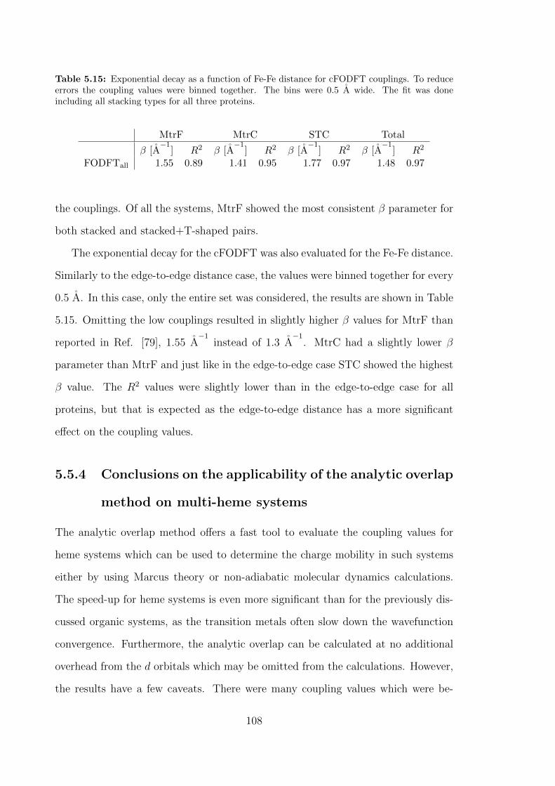
Table 5.15: Exponential decay as a function of Fe-Fe distance for cFODFT couplings. To reduceerrors the coupling values were binned together. The bins were 0.5 A wide. The fit was doneincluding all stacking types for all three proteins.
MtrF MtrC STC Total
β [A−1
] R2 β [A−1
] R2 β [A−1
] R2 β [A−1
] R2
FODFTall 1.55 0.89 1.41 0.95 1.77 0.97 1.48 0.97
the couplings. Of all the systems, MtrF showed the most consistent β parameter for
both stacked and stacked+T-shaped pairs.
The exponential decay for the cFODFT was also evaluated for the Fe-Fe distance.
Similarly to the edge-to-edge distance case, the values were binned together for every
0.5 A. In this case, only the entire set was considered, the results are shown in Table
5.15. Omitting the low couplings resulted in slightly higher β values for MtrF than
reported in Ref. [79], 1.55 A−1
instead of 1.3 A−1
. MtrC had a slightly lower β
parameter than MtrF and just like in the edge-to-edge case STC showed the highest
β value. The R2 values were slightly lower than in the edge-to-edge case for all
proteins, but that is expected as the edge-to-edge distance has a more significant
effect on the coupling values.
5.5.4 Conclusions on the applicability of the analytic overlap
method on multi-heme systems
The analytic overlap method offers a fast tool to evaluate the coupling values for
heme systems which can be used to determine the charge mobility in such systems
either by using Marcus theory or non-adiabatic molecular dynamics calculations.
The speed-up for heme systems is even more significant than for the previously dis-
cussed organic systems, as the transition metals often slow down the wavefunction
convergence. Furthermore, the analytic overlap can be calculated at no additional
overhead from the d orbitals which may be omitted from the calculations. However,
the results have a few caveats. There were many coupling values which were be-
108

low the precision of cFODFT which makes their estimation difficult. Also while the
ERMSLEs of the heme systems were almost comparable to those reported in Sec-
tion 5.1 the spread of the RMS(Hab) vs. RMS(Sab) was much wider. In general, the
errors were larger when smaller couplings were also included. In dense systems, such
as organic semiconductors, where the mobility is dominated by the largest coupling
values the inaccuracy in calculating small couplings is not a serious issue, but it can
be a significant problem in proteins where the smallest coupling values can act as
bottleneck.
Most of this inaccuracy comes from the fact that the idealised heme structures
are used for the overlap calculation which does not necessarily describe well the MD
snapshots where the large fluctuations of the heme structure alters the SOMO and
SOMO-1 pairs. If the method is to be used to calculate coupling values the results
can be improved if instead of one set of STO expansion coefficients a handful of them
are used which were obtained for a set of sample structures. Then, a random MD
snapshot can be fitted to the most appropriate element of the sample using a more
tailored coefficient set instead of one-set-fits-all. It would also be interesting to see
how FODFT and FODFTB values compare in this case however it maybe difficult
to converge the same orbital with FODFTB [124].
5.6 Non-adiabatic coupling vector element calcu-
lations with the fast overlap code
The overlap method can be applied to address another element in the non-adiabatic
transport model. As was shown in Chapter 3 in Eq. (3.23), in order to propagate
the excess electron in the system, the Hamiltonian matrix elements Hkj and the non-
adiabatic coupling elements 〈φk|dφjdt〉 have to be calculated. While the former has
been addressed extensively in this chapter, the latter is more difficult to calculate.
In this section, a possible approximation of the non-adiabatic coupling is presented
109
using the analytic overlap method.
Applying the chain rule, the non-adiabatic coupling can be expressed as a dot
product of the nuclear velocity vector R and the non-adiabatic coupling vector
〈φk|∇Rφj〉,
〈φk|dφjdt〉 = R · 〈φk|∇Rφj〉. (5.21)
In order to calculate the non-adiabatic coupling elements, the nuclear velocity can
be obtained from the molecular dynamics while the non-adiabatic coupling vector
(NACV) can be expressed using a finite difference method:
〈φk|∇Rφj〉 ≈ 〈φk(R)|φj(R + δR)− φj(R)
δR〉 (5.22a)
〈φk|∇Rφj〉 ≈〈φk(R)|φj(R + δR)〉
δR− 〈φk(R)|φj(R)〉
δR(5.22b)
〈φk|∇Rφj〉 ≈SR,R+δR − SR,R
δR(5.22c)
where φj(R + δR) is the wavefunction where the excess electron is localised on site
j and the nuclear structure is distorted by δR. This 2-point scheme approximates
the non-adiabatic coupling vector to be proportionate to the difference between the
overlap of one distorted and one undistorted molecule and two undistorted molecules.
5.6.1 Assumptions of the NACV calculation with AOM
As the finite difference model yielded a solution that is a linear combination of
overlaps, the fast overlap method can provide a framework to calculate the NACVs.
However, considering the computational challenges of the NACV calculation and the
limitation of the fast overlap method, it is crucial to understand the approximations
made here.
In a donor-acceptor system where the donor has N atoms and the acceptor has
M atoms the NACVs 〈φk|∇Rφj〉 and 〈φj|∇Rφk〉 have a total number of 3M + 3N
110

components, including all atoms of the acceptor and the donor in all three possible
directions. Using Eq. (5.22c), this means that 3× (N +M) + 1 overlap calculations
are performed including SR,R.
Like in the preceding chapters, non-orthogonal localised states give an intuitive
framework to understand the components of the expression but the reference wave-
function has to be derived from an SCF calculation. Using fragment orbital based
methods to obtain the coefficients avoids polarisation effects and reduces the number
of wavefunctions to be calculated. For example, the wavefunction in state k (approx-
imated as SOMO of the donor) is unchanged when the distortion δR only happens
to the nuclear structure of the acceptor molecule and vice versa. This means that
the undistorted wavefunctions on the acceptor and the donor, denoted as φA(R) and
φD(R) respectively, are the same in each calculation. As a consequence, the number
of localised wavefunctions which have to be calculated is 3 × (N + M) + 2. In the
AOM case, the SOMO is projected onto the STO basis set. Following the steps of
the Sab calculation in Section 5.1, the φj(R + δR) can be obtained by performing an
SCF calculation followed by a Kohn–Sham diagonalisation for every 3× (N+M)+2
structure. However, this would create a serious overhead which would reduce the
advantage gained from replacing FODFT with AOM and would make it impossible
to be used in non-adiabatic molecular dynamics simulations.
To avoid the orbital calculation overhead, the following assumptions were ap-
plied: since δR is small so is the change in the orbital coefficients and the main
difference comes from the fact that the centre of the orbital is displaced. Hence, the
same coefficients are used which were derived from the undistorted structure. These
coefficients are normalised for the distorted structure and the overlap between the
distorted and undistorted molecule is calculated for each component of the NACV.
The algorithm performs the following steps:
• Calculate the overlap between the undistorted structures of the donor and
acceptor molecules SDA ≡ SR,R
111

• Define δRi,r where i = 1 . . . N +M and r = x, y, z
• Distort atom i of the molecule in direction r structure (R + δRi,r).
• Reconstruct orbital on distorted molecule using the coefficients of the undis-
torted molecule c.
• Renormalise coefficients on distorted molecule c −→ c′i,r.
• Calculate overlap between distorted donor molecule and undistorted acceptor
molecule (SR,R+δRi,r).
• Calculate relevant NACV elements according to Eq. (5.22c).
• Loop over all atoms of the dimer in all directions (every possible value of i and
r).
This way the 3×(N+M) NACV components can be calculated without obtaining
the orbital for each distorted structure, as long as the approximations hold.
5.6.2 Validation
Clearly, the overlap method for NACV calculation is only useful if the assumptions
with respect to the wavefunctions provide a good approximation to higher level solu-
tions. An SCF comparison can be used to assess the effects of the orbital relaxation.
Polarisation between the monomers was omitted here as well and, to be consistent
with the previous sections, FODFT benchmarking was chosen with simulation details
identical to those in Section 4.3.
For testing purposes parallelly stacked ethylenes were used at 3.5 A, 4.5 A, and
5.0 A stacking distance. Since 2×3×N calculations have to be performed a smaller
system is a better choice, as the computational requirements are lower. The sym-
metric configuration also allowed us to check whether the program reproduces the
symmetry of the system. Furthermore, since the errors of the AOM have been tested
112
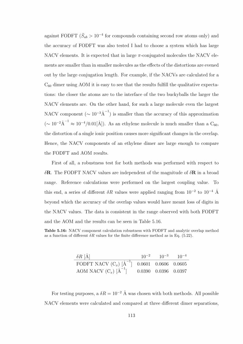
against FODFT (Sab > 10−4 for compounds containing second row atoms only) and
the accuracy of FODFT was also tested I had to choose a system which has large
NACV elements. It is expected that in large π-conjugated molecules the NACV ele-
ments are smaller than in smaller molecules as the effects of the distortions are evened
out by the large conjugation length. For example, if the NACVs are calculated for a
C60 dimer using AOM it is easy to see that the results fulfill the qualitative expecta-
tions: the closer the atoms are to the interface of the two buckyballs the larger the
NACV elements are. On the other hand, for such a large molecule even the largest
NACV component (∼ 10−3A−1
) is smaller than the accuracy of this approximation
(∼ 10−2A−1≈ 10−4/0.01[A]). As an ethylene molecule is much smaller than a C60,
the distortion of a single ionic position causes more significant changes in the overlap.
Hence, the NACV components of an ethylene dimer are large enough to compare
the FODFT and AOM results.
First of all, a robustness test for both methods was performed with respect to
δR. The FODFT NACV values are independent of the magnitude of δR in a broad
range. Reference calculations were performed on the largest coupling value. To
this end, a series of different δR values were applied ranging from 10−2 to 10−4 A
beyond which the accuracy of the overlap values would have meant loss of digits in
the NACV values. The data is consistent in the range observed with both FODFT
and the AOM and the results can be seen in Table 5.16.
Table 5.16: NACV component calculation robustness with FODFT and analytic overlap methodas a function of different δR values for the finite difference method as in Eq. (5.22).
δR [A] 10−2 10−3 10−4
FODFT NACV (Cx) [A−1
] 0.0601 0.0606 0.0605
AOM NACV (Cx) [A−1
] 0.0390 0.0396 0.0397
For testing purposes, a δR = 10−2 A was chosen with both methods. All possible
NACV elements were calculated and compared at three different dimer separations,
113
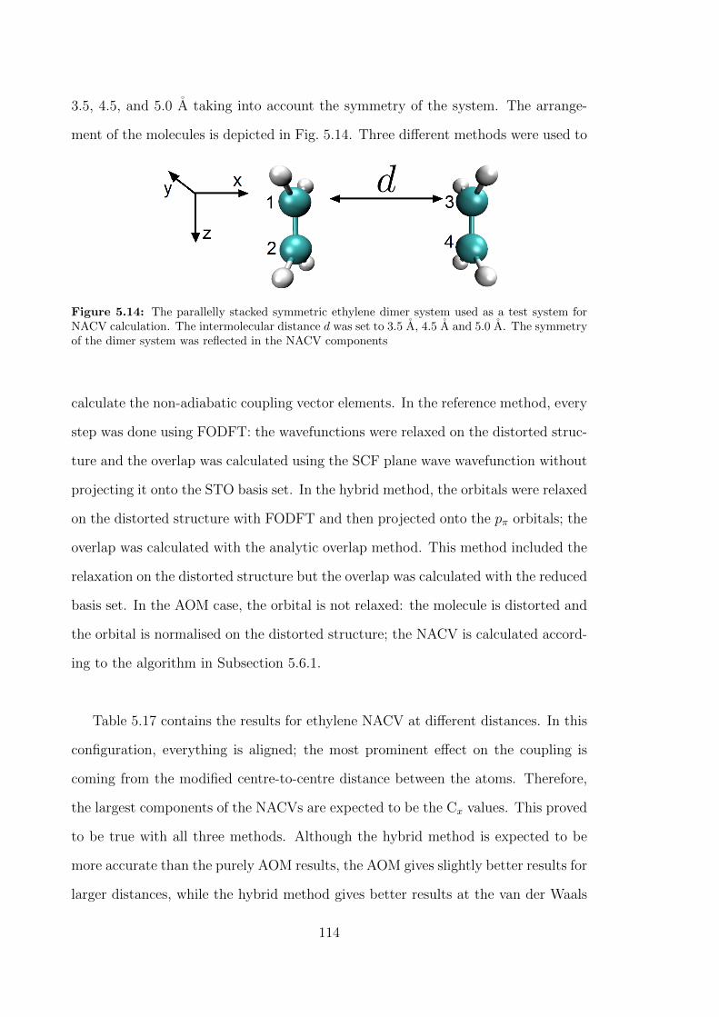
3.5, 4.5, and 5.0 A taking into account the symmetry of the system. The arrange-
ment of the molecules is depicted in Fig. 5.14. Three different methods were used to
Figure 5.14: The parallelly stacked symmetric ethylene dimer system used as a test system forNACV calculation. The intermolecular distance d was set to 3.5 A, 4.5 A and 5.0 A. The symmetryof the dimer system was reflected in the NACV components
calculate the non-adiabatic coupling vector elements. In the reference method, every
step was done using FODFT: the wavefunctions were relaxed on the distorted struc-
ture and the overlap was calculated using the SCF plane wave wavefunction without
projecting it onto the STO basis set. In the hybrid method, the orbitals were relaxed
on the distorted structure with FODFT and then projected onto the pπ orbitals; the
overlap was calculated with the analytic overlap method. This method included the
relaxation on the distorted structure but the overlap was calculated with the reduced
basis set. In the AOM case, the orbital is not relaxed: the molecule is distorted and
the orbital is normalised on the distorted structure; the NACV is calculated accord-
ing to the algorithm in Subsection 5.6.1.
Table 5.17 contains the results for ethylene NACV at different distances. In this
configuration, everything is aligned; the most prominent effect on the coupling is
coming from the modified centre-to-centre distance between the atoms. Therefore,
the largest components of the NACVs are expected to be the Cx values. This proved
to be true with all three methods. Although the hybrid method is expected to be
more accurate than the purely AOM results, the AOM gives slightly better results for
larger distances, while the hybrid method gives better results at the van der Waals
114

distance (3.5 A). Of course this does not mean that AOM is a better approach;
this effect is more likely due to error cancellation. The x components had a MRUE
of 26% and MAXERR of 0.02 A−1
with the hybrid method, and 19% MRUE and
0.03A−1
MAXERR with AOM. The AOM error was strongly distance dependent
and gave the best approximation at 4.5 A with less than 3% error. Basically, the
results are very good with both methods. The effects of the orbital relaxation is
negligible. Cy values are not indicated in any of the cases as they are well below the
accuracy of the method (0.01 A−1
) even at 3.5 A distance.
The Cz components showed a much larger deviation from the FODFT results with
relative errors of 82% for the hybrid method and 92% for the AOM. The results are
an order of magnitude off from the FODFT method with both approximate methods.
In the z direction, the hybrid method gives consistently better results than the AOM
at all distances. This means that in this case, the differences partially arise from the
relaxation of the orbital on the distorted structure. However, as the hybrid method
does not fully account for the change even when s orbitals are included in the overlap,
there is another underlying effect. A possible explanation is that since these values
are small, this might be the limit of accuracy with which the FODFT results can be
reproduced, the effects of the distortion in the z direction cannot be well projected
onto the minimum STO basis set.
As expected, the contribution of the H atoms were all below the precision of the
presented methods, therefore they are not discussed. It is worth noting however, that
in the FODFT approximation displacing the H atoms slightly alters the shape of the
SOMO causing the NACV components to be non-zero. In the AOM algorithm, the
orbital is not SCF optimised and since only the pπ orbitals are taken into account
the H atoms do not contribute explicitly to the overlap (not even when s orbitals are
taken into account). On the other hand, the positions of the H atoms have an implicit
effect on the orbital shape as their displacement can alter the pπ directions on the C
115

Table 5.17: NACV calculations with three different methods at different dimer separations on aperfectly stacked ethylene dimer. In the case of the reference FODFT method, the wavefunctionis relaxed on the distorted structure and the overlap is calculated between the full orbitals. Thehybrid method relaxes wavefunctions which are projected onto the minimum STO basis set andcalculates the overlap analytically. The AOM uses the undistorted STO coefficients and calculatesthe overlap analytically. The results are calculated at different distances. The letters refer to thetype of atom and the direction of the NACV element.
separation method Cx,1 = Cx,2 Cz,1 ≈ −Cz,2
3.5 A
Ref. (FODFT )[A−1
] 6.01×10⁻² 3.95×10⁻²
Hybrid[A−1
] 4.14×10⁻² 5.77 ×10⁻³
AOM [A−1
] 3.43 ×10⁻² 3.14×10⁻³
4.5 A
Ref. (FODFT )[A−1
] 2.18×10⁻² 2.00×10⁻²
Hybrid[A−1
] 1.69×10⁻² 3.80×10⁻³
AOM [A−1
] 2.13×10⁻² 1.19×10⁻³
5.0 A
Ref. (FODFT )[A−1
] 1.30×10⁻² 1.36×10⁻²
Hybrid[A−1
] 9.80×10⁻³ 2.65×10⁻³
AOM [A−1
] 1.45×10⁻² 1.42×10⁻³
atoms. Consequently, by moving the H atoms in the plane of the conjugation (y and
z directions in this configuration), the pπ directions on the C atoms are unchanged
and therefore the overlap as well, resulting in 0.00 Hy and Hz components. This is
true for all NACV elements when the AOM code is used on a compound which have
atoms which do not participate in the π-conjugation.
5.6.3 Conclusion of NACV calculation with the AOM
It was shown how the analytic overlap method can be used to approximate the non-
adiabatic coupling vector elements for π-conjugated systems using the example of
the ethylene dimer for which the NACV values were fairly accurate. Since all other
conjugate systems are larger the absolute error in NACV calculations is expected
to decrease. It was also demonstrated that the results are more accurate in the
stacking direction but are consistently underestimated along the bond direction by
an order of magnitude which is expected to be due to the limited STO basis set.
116
This, however, might not be such a significant issue as the accuracy of the derived
NACV elements can be measured best by analysing their effect on the non-adiabatic
molecular dynamics simulations. Most of the times, the effect of NACV is negligible
but they gain importance at the crossing of the diabatic surface. Off-diagonal forces
can also be derived from the NACVs as
∇Hkj ≈ C · ∇Skj = C · (〈φj|∇Rφk〉∗ + 〈φk|∇Rφj〉) (5.23)
In this case, the two directions are not equal. In the x direction both components are
pointing in the direction of the other monomer pushing them together, while in the
z direction the off-diagonal forces point towards one another along the bond. These
derived off-diagonal forces are around 1.3×10⁻³ a.u. along the bond which is two
orders of magnitude smaller than the C=C spring constant, therefore the effects are
negligible. The NACV component along the covalent bond is expected to be even
smaller for molecules larger than ethylene. Therefore, it is expected that the error
made for this component will not have a significant effect in non-adiabatic molecular
dynamics runs.
5.7 Further speed-up
The fast analytic overlap method also introduces another opportunity to make the
scheme linearly scaling with molecule size through the introduction of a cut-off for
the calculation of atomic orbital pair overlaps. This can improve the speed-up for
larger molecules. There are two options: the cut-off can be distance dependent; in
this case the overlap is calculated only between atoms of the acceptor an the donor
which are not further than a certain rmax distance. Another way is to calculate the
overlap between those atoms for which the atomic overlap is expected to be larger
than the threshold sminab and all other components of the atomic overlap matrix is set
117

to 0. The benefits of the first method is rather trivial. The second method, termed
here as minimum atomic overlap method, becomes very useful if AOM is used within
NAMD simulations. During dynamics, the overlap and NACV values are changing
slowly compared to the time resolution. For the minimum atomic overlap method
an atomic neighbour list can be created for each molecular dimer which tells which
atom pairs fulfill the criterion sab > sminab . This list can be updated once the nuclear
motion is significant enough to make changes to the overlap. The two methods are
expected to be in general rather similar as the atomic overlap is strongly dependent
on the interatomic distance. The minimum interatomic overlap method becomes
useful when the molecules have a complex nodal structure. In this case, it could
be that although two atoms are close to one another but the overlap is negligible
because the orbitals of those atoms hardly contribute to the SOMO. In this case,
while the overlap is still calculated in the minimum interatomic distance method in
the minimum atomic overlap method these calculations are set to 0.
In terms of computational time, the cut-off makes no difference for small systems
but larger molecules such as C60 benefit from it significantly. This implementation
uses the minimal inter-atomic overlap criterion method. The effects of a reduced
atomic overlap calculation can be seen in Table 5.18.
For atomic overlap cut-offs greater than 10−6 increasing amount of NACV ele-
ments became exactly zero. Despite this, there is no significant change in the value
of the largest component which is dominated by the larger atomic overlap values.
The cut-off can be applied generously for C60, as expected the coupling values are
affected mostly by the atomic overlaps of a few atoms closest to the interface of the
monomers. The accuracy of the smaller coupling value was preserved better than
the larger one. When the atomic overlap cut-off is set to 10−2 the overlap and all
NACV components become 0.
118

Table 5.18: Different atomic overlap cut-offs, and their effect on the overlap calculation accuracyand computational time demonstrated on two C60 dimers one with a large overlap value, andanother one with a small one.
sminab Sab CPU time [s] NACV [A
−1] CPU time [s]
high coupling C60
none 7.029× 10⁻³ 0.00257 1.91× 10⁻³ 0.164510−8 7.029× 10⁻³ 0.00161 1.92× 10⁻³ 0.139810−6 7.051× 10⁻³ 0.00077 1.92× 10⁻³ 0.106610−5 6.859× 10⁻³ 0.00040 1.92× 10⁻³ 0.077610−4 7.642× 10⁻³ 0.00018 1.92× 10⁻³ 0.047810−3 2.661× 10⁻³ 0.00010 2.92× 10⁻³ 0.0375
low coupling C60
none 1.930× 10⁻⁵ 0.00270 1.83× 10⁻³ 0.157910−8 1.931× 10⁻⁵ 0.00149 1.83× 10⁻³ 0.125810−6 1.940× 10⁻⁵ 0.00074 1.83× 10⁻³ 0.104510−5 9.741× 10⁻⁶ 0.00040 1.82× 10⁻³ 0.077110−4 1.576× 10⁻⁵ 0.00017 1.67× 10⁻³ 0.045810−3 1.727× 10⁻⁵ 0.00011 1.58× 10⁻³ 0.0413
5.8 Conclusion
It was demonstrated in this chapter that the electronic coupling matrix elements
between π-conjugated organic molecules scale approximately linearly with the over-
lap between the singly occupied molecular orbitals in the range relevant to electron
transport in the condensed phase (5 to 500 meV). It was also shown that a single
proportionality constant can describe a broad set of molecules, and the accuracy
is retained when the basis set is replaced with the minimum STO basis set with
optimised Slater decay coefficients.
This also provides a tool to estimate electronic couplings analytically, leading
to speed-ups of approximately six orders of magnitude compared to standard DFT
calculations for molecules typically used in molecular OSCs. The analytic overlap
119

method can also be used to estimate off-diagonal elements of the Hamiltonian in
NAMD simulations of charge transport where further speed-up is possible when
atomic overlap cut-off is used.
The analytic overlap method offers a fast option for evaluating the coupling
values which can be used to determine the charge transport using Marcus theory as
well. This was demonstrated on a set of heme systems where the effect of molecular
dynamics was also taken into account. The convenience of omitting the d orbitals and
using the optimised coefficients offers a reasonable approximation for the coupling
values and saves computational time. Here, the main issue is the magnitude of the
Hab values. Heme systems often have coupling values less than 1 meV which makes
them prone to error with the AOM. Furthermore, hemes are non-rigid molecules. In
particular, the rotation of the histidine molecules has a very low energy barrier. This
causes large fluctuations in the orbitals which make the overlap deviate significantly
from the values calculated with the idealised orbital coefficients. These two effects
can lead to large errors in charge transport modelling as in proteins electron transfer
is often dominated by the smallest coupling, which acts as a bottleneck for the
process. Although in its current form the model may not be ideal for calculating
rates in non-adiabatic molecular dynamics, it is possible to adapt the model to tackle
the issue by defining multiple coefficient sets based on a set of reference molecular
conformations of hemes. Molecular dynamics snapshots of heme molecules can be
fitted to these reference sets by minimising the root-mean-square distance between
the molecules and finding the best fit. The orbital coefficients of the best fitting
reference molecules can be used on the MD snapshot hemes.
The analytic overlap method can also be used to approximate the non-adiabatic
coupling vector elements for π-conjugated systems. This was demonstrated on the
ethylene dimer. The NACV component pointing from one molecule to the other
could be reproduced well compared to FODFT reference calculations. Although the
results were not so good along the bonds, this is not an issue as the nuclear forces
120
arising from the off-diagonals of the Hamiltonian are two orders of magnitude smaller
than the nuclear forces in the same direction. Since all other conjugated systems
are larger than an ethylene molecule the absolute value of the NACV components
are smaller. Therefore, the absolute error in the off-diagonal forces is expected to be
even smaller for OSC molecules.
121
6 Kinetic Monte Carlo simulations
for charge carrier hopping
In Chapter 3, the various parameters required to simulate charge transport in organic
systems were discussed and Chapters 4 and 5 were focusing on the calculation of the
electronic coupling matrix elements and the non-adiabatic coupling vector elements
in different systems with various methods.
As mentioned in Chapter 2, the role of dynamic disorder in organic semiconduc-
tors can be very significant. This is especially true for fullerene crystals as discussed
in Refs. [45, 49]. Chapter 5 discussed the applicability of the analytic overlap method
in heme systems which were extracted from molecular dynamics trajectories. For
these systems a few issues arose from the small coupling values and the orbital
fluctuations due to intramolecular deformations. However, the relatively limited
movements of the heme systems did not cause a significant change in the individual
couplings over time, and the magnitude of the coupling fluctuations remained small
throughout the trajectory [79].
As discussed previously, localised transport is not applicable in many organic
systems. In some cases, this is due to the fact that the energy barrier between the
two states disappears and the charge carrier no longer forms localised polarons. In
other cases, the partial delocalisation is due to dynamic effects, as the molecular
motion affects the couplings and can create clusters of delocalised states.
Non-adiabatic molecular dynamics provides a tool which allows charge transport
simulation in those systems which are partially delocalised. However, in those sys-
tems where localised transport is applicable, rate equation-based charge transport
122

models provide a faster solution. To this end, understanding the timescales of dif-
ferent parameters which contribute to the transport is crucial for developing better
models. This chapter presents the application of the analytic overlap method in
a localised transport model where a rate equation is used to determine the charge
transport (the basic theoretical underpinnings of which were discussed in Chapter
3). It goes on to present a practical implementation to obtain mobility values by
using the rate equation in combination with a kinetic Monte Carlo program. The
first half of the chapter presents the details of the implementation in particular, the
calculation of various components of the rate equation such as the electronic coupling
matrix element, the reorganisation energy, and the nuclear tunneling frequency. The
second half of this chapter discusses the dynamic effects in organic systems and the
separation of time scales of different parameters relevant to localised transport.
6.1 Implementation
As mentioned in Chapter 3, rate equation based transport can be described as Marko-
vian process. This means that between each hop the electron thermalises and the
system has no memory. Therefore the hop from state (site) i to state (site) i+1 only
depends on state (site) i and has no memory of state (site) i− 1. Electron hopping
from site to site is a discrete Markovian process as the possible states are countable.
The time evolution of such systems can be described with the master equation
dP
dt= A(t)P(t) (6.1)
where P is the time dependent probability vector of the electron being in a given
state and A is the connection matrix depending on time depndent rate constants.
Monte Carlo models also offer a solution. The kinetic Monte Carlo code presented
here uses the generalised rate expression, Eq (3.16) from Ref [45], which interpo-
123
lates between non-adiabatic and adiabatic charge transfer expressions. This rate
expression requires the electronic coupling matrix element between the molecules of
interest, the reorganisation energy, the free energy difference between the hopping
sites, and the effective nuclear frequency along the reaction coordinate. The elec-
tronic coupling matrix elements are calculated using the analytic overlap method
code described in Chapter 5 which is called by the kinetic Monte Carlo code I have
written.
The electron is propagated using the Borz–Kalos–Leibowitz algorithm which is a
no-rejection Monte Carlo algorithm. This algorithm requires two random numbers
per hop [125, 126]. The first random number drawn, r1 ∈ (0, 1], determines the
residence time at the current site i before it hops to the an adjacent site with the
equation
tstay = − 1
kiln(r1). (6.2)
where ki =∑
j kij is the sum of the hopping rates between site i and its nearest
neighbours. A second random number r2 ∈ (0, 1] is generated to determine the
hopping direction. The interval (0, 1] is divided into n intervals, where n is the
number of neighbours for given site, and the size of these intervals is proportional
to the magnitude of the hopping rates to each neighbouring site. The region which
contains r2 indicates the hopping direction. After each hopping step the system
time is updated by tstay and the displacement of the electron is updated by the
displacement vector between the new site and the previous site. Periodic boundary
conditions are applied to avoid finite size effects. Each KMC trajectory is terminated
when the system time reaches a given maximum simulation time which is specified
in the input file. The final displacement compared to the initial site and the system
time are dumped into separate output files. To ensure ergodicity, the initial site
for each trajectory is randomly chosen according to uniform distribution, assuming
that the injected electron has a much higher energy than any of the sites. Although
124
the code itself does not perform molecular dynamics it can be used to study the
dynamics in the system by loading trajectories obtained from molecular dynamics
done with other packages such as AMBER or NAMD.
6.1.1 Rate calculation
To support this model, a suitable rate expression had to be used. For the rate
calculation, the generalised rate expression Eq. (3.16) is used, of which the non-
adiabatic (3.12) and the adiabatic (3.13) rate are limits in special cases
k = κelνnΓ exp(−(∆A†/kBT ))) (6.3)
In order to calculate the rates, the activation free energy, the electronic coupling
elements, the reorganisation energy, and the effective nuclear frequency have to be
obtained for this model system.
Reorganisation energy
The reorganisation energy was calculated according to Marcus and consists of an
inner-sphere contribution λi and an outer-sphere contribution λo [42],
λ = λi + λo (6.4)
The inner sphere contribution is calculated using the four-point scheme
λi = (EC(RN) + EN(RC)− (EC(RC + EN(RN)) (6.5)
The terms in the sum come from four single point SCF energy calculations with
simulation details analogous to the ones presented for fullerenes in Section 5.3. The
optimised charged (RC) and neutral (RN) configurations were the same as the ones
presented in Table 6.1. EC refers to single point calculation for a charged molecule
125

and EN refers to a neutral single point calculation. This is only calculated for one
pair of SCF minimised molecules, it is expected that the inner sphere contribution
does not change substantially throughout the charge transport process at finite tem-
peratures. The outer-sphere contribution was estimated with the Marcus formula
taking into account the effect of the polarisability of the surrounding molecules
λo = (∆q)2
(1
εop
− 1
εs
)(1
r− 1
R
), (6.6)
where r = 5.02 A is the van der Waals radius of the C60 cage. εop and εs are
optical and static experimental dielectric constants [127, 128], R is the intermolecular
distance and ∆q is the charge difference. The polarisable sphere model works well
for the C60 molecules but it can introduce errors for elongated molecules such as
pentacene. Therefore, the outer-sphere contribution is optional in the code.
Free energy calculation
The free energy values were obtained from molecular dynamics calculation. To be
comparable with the DFT results, the molecular dynamics force field parameters were
altered to reproduce the charged and neutral bond lengths of C60 in Table 6.1 and the
λi value obtained by DFT according to Eq. (6.5). The MD simulation is done in an
NVT ensemble where all molecules are neutral. Then, using this neutral trajectory,
the energies are evaluated again by making each molecule charged, simulating that
the electron is in a given configuration during the entire trajectory but with an
unchanged geometry, and thus obtaining the vertical energy difference between the
charged and the neutral state ∆E.
∆Ei = EC,i(RN)− EN(RN) (6.7)
where EC,i is the energy value for a given snapshot when the electron is located on
site i and RN refers to the nuclear coordinates of the entire neutral trajectory.
126
The free energy calculation can be obtained by using the Landau free energy term
[41]. However, since there are no solvents included the expected energy landscape
has rather sharp peaks. The free energy is calculated as the thermal average of the
obtained vertical energy differences for a given site i.
∆Ai = −kBT log
(∑i
exp (∆Ei/kBT )
)(6.8)
Since the reorganisation energy values are fairly uniform and small in small molecule
organic semiconductors the free energy difference between two sites can be calculated
as
∆Aij = ∆Ai −∆Aj (6.9)
Of course, for identical molecular sites within the crystal, ∆Aij = 0. The energy in
the condensed phase is expected to be dominated by the intramolecular terms as the
polarisation effect of the surroundings is expected to be less significant in organic
semiconductors than in solutions [79].
Coupling calculation
Given the number of coupling calculations one has to perform for a molecular dy-
namics trajectory, the analytic overlap method can be used to approximate the Hab
values. As was shown on the example of the heme system, the coupling values ob-
tained with the SCF minimised ionic structure provided a reasonable approximation
for coupling values in molecular dynamics trajectories as long as the coupling values
are sufficiently large. For C60, the couplings for the nearest neighbours are expected
to range between 1 to 100 meV. Furthermore, crystalline C60 is a dense system in
which the charge transport is dominated by the largest coupling values. Since AOM
was tested on the fullerene system and can tackle the large number number of cal-
culations it is going to be used in this model with the linear scaling factor for Eq.
(5.1) obtained in Chapter 5 of C = 1819 meV.
127

In order to address orbital degeneracy, the level of degeneracy can be specified
in the input file and the overlap values are averaged according to Eq. (5.19) [123].
Effective nuclear frequency
The effective nuclear frequency along the reaction coordinate can also be obtained
by analysing the time dependence of the vertical energy gap. This is done by un-
derstanding that in the diabatic representation, the charge transition happens when
the vertical energy gap vanishes [129]. Using linear response theory, the effective
nuclear frequency can be obtained by taking the weighted average of the spectral
density function of the vertical energy gap calculated in the classical MD [41],
2πνn =
∫∞0ω J(ω)
ωdω∫∞
0J(ω)ω
dω(6.10)
where J(ω)/ω is the spectral density function calculated as
J(ω) =ω
2kBT
∫ ∞0
c(t) cos(ωt)dt (6.11)
where c(t) is the time-correlation function of the vertical energy gap difference be-
tween two sites ∆Eij
c(t) = 〈∆Eij(0)∆Eij(t)〉 (6.12)
Eq. (6.12) describes time-dependent behaviour of the system on the diabatic poten-
tial energy surface and is used here to understand how often the system gets close to
the transition point (∆Eij = 0). In the case of small molecule organic semiconduc-
tors, this is expected to be dominated by the intramolecular vibrations which show
up as sharp peaks on the energy spectrum and the spectral density function.
As mentioned in Chapter 3, the localised transport model is only applicable if
the activation free energy is positive, and therefore there is a finite energy barrier
128
between the two localised states. To this end, it can be easily seen in Eq. (3.16)
that the localised charge transport can only be used if the coupling is smaller than
3/8 of the reorganisation energy. In order to avoid issues arising from negative acti-
vation energy, in this implementation ∆A† is set to zero when it would be otherwise
negative.
6.1.2 Calculating the charge carrier mobility
Three methods are presented in this chapter to calculate the charge carrier mobility
µ and are compared for the systems to assess the accuracy of the calculations.
Analytical derivation of µ
The first method does not actually rely on Monte Carlo results. The obtained rates
are used to approximate the drift velocity as the average of the sum of the rates knm
multiplied by the corresponding translation vector rnm as in Ref. [45]. In a unit cell
consisting of N molecules, this can be averaged for the unique sites
vdrift =1
N
N∑n=1
∑m
knmrnm (6.13)
where m sums over the possible neighbours of site n . In order to obtain the mobility
matrix, the derivative of each velocity component of vdrift, vdrift,i, i = x, y, z is taken
with respect to the electronic field E in direction j, Ej, j = x, y, z the mobility is
then
µij =∂vdrift,i
∂Ej=∂(
1N
∑n
∑m knmrnm
)i
∂Eji, j = x, y, z (6.14)
Here, the external field is assumed to be small enough so it does not have a significant
effect on the dynamics. Therefore, rnm is independent of the external field E. Thus,
the drift velocity only depends on the external field as specified in rate equation
Eq. (3.16), where the potential energy difference between two sites in the presence
129

of external field is
∆A = −qeE · r + ∆As (6.15)
where ∆As is the static free energy difference between the two sites. Inserting the
rate expression Eq. (3.16) into Eq. (6.14) and evaluating the derivative with respect
to Ej gives
µij =1
N
∑n
∑m
rnm,i∂knm∂Ej
=1
N
∑n
∑m
DijnmknmkBT
(6.16)
where kB is the Boltzmann constant, T is the temperature, and Dijnm is given by
Dijnm =ernm,irnm,j
2
(1 +
(2Hnm
λ− eEjrnm,j
)2)−1/2
− eEjrnm,jλ
(6.17)
In order to obtain mobility values according to this approximation, the knowledge of
every coupling value, displacement, and site energy value in the system is required.
However, as this mobility value does not depend on the kinetic Monte Carlo results,
it can be used to assess if the kinetic Monte Carlo results have converged as long as
the system size is reasonable.
Mobility values from Einstein relation
One way to calculate the mobility using the kinetic Monte Carlo results is through
exploiting the Einstein relation,
µ =qD
kBT(6.18)
This is valid when the hopping process is well described by a diffusion process, i.e.
the medium is isotropic for a given direction (in the positive and negative directions)
and the hops are stochastic. The KMC results can be used to obtain the diffusion
coefficient D. In the three dimensional case, the probability density of the localised
charge movement is
P (R, t) = C(det(D)) exp(−RTD−1R
4t). (6.19)
130

where C(det(D)) is a normalisation factor, R is the displacement vector, t is time
and D is the diffusion tensor. D can be determined by taking the slope of the mean
square displacement of the particle as a function of time t. In the three dimensional
case, this is obtained by taking the covariance matrix of the displacement as
〈(Ri − 〈Ri〉)(Rj − 〈Rj〉)〉 = cov(Rij) = 2Dijt, (6.20)
where i, j = x, y, z. Thus, the mobility tensor can be calculated as
µij =qcov(Rij)
kBT2t. (6.21)
It is worth noting that this approximation can only be used if the R2 values are
sufficiently large when the components of cov(Rij) are plotted as the function of t.
Mobility values from numerical derivative
By definition, the mobility can be obtained as the derivative of the drift velocity
with respect to the external field,
µij =∂vdrift
∂E=
vjdrift(E + δEi)− vjdrift(E− δEi)
2δEi, j = x, y, z (6.22)
where i and j are unit vectors in the directions x, y, and z.
6.2 Validation
The KMC code was tested with a single perfectly aligned crystalline C60 system to
assess the convergence criteria. The fcc crystal had a lattice constant of 14.01 A and
each site was equivalent with zero potential energy difference. Every molecule was
rotationally equivalent; the co-rotating internal coordinate system of the buckyballs
was aligned with the external coordinate system. The maximum hopping distance
131

and thus the cut-off for the rate calculation was 12 A which included the nearest
neighbours only.
The convergence of the electronic mobilities in the test system was validated with
respect to the number of KMC trajectories, temperature, and overlap conversion
factor. The electron mobilities were calculated with all three different methods where
applicable: Einstein relation for Brownian motion Eq. (6.18), analytical derivative
of the drift velocity according to Eq. (6.16), and numerical derivative of the drift
velocity with respect to the external field as in Eq. (6.22).
Figure 6.1: Convergence of the mobility values calculated with the finite difference method as inEq. (6.22) and Eq. (6.18) to the analytically obtained mobility value as a function of the numberof Monte Carlo trajectories. The results start to converge at around 5×10⁵ trajectories. Usingmore KMC trajectories changes the mobility values by less than 0.05 cm2/Vs. It can be seen herethat the Einstein mobility values are slightly overestimating the numerical and analytical derivativeresults and the effect is stronger for larger couplings.
132

The results of the KMC code were compared to the analytic results obtained
from Eq. (6.16). The simulation showed that 5×10⁵ individual KMC trajectories for
a single snapshot are enough to reach convergence to the accuracy of 0.05 cm2/Vs
both with the finite difference method and the Einstein relation, as can be seen in
Fig. 6.1. The code was less sensitive to the simulation time t. Convergence was ob-
tained even when the simulation time was so short that only a few events happened.
Furthermore, even at short simulation times of t = 10−12 s the 〈x2〉 vs. t plot was
a straight line with R2 = 0.9997 which started to deviate from the straight line at
shorter simulation times.
Figure 6.2: External electric field dependency of the electron mobility with different offsets usingδE = 104 V/cm. The mobility was evaluated with the analytic derivative method (Eq. (6.16)) andthe numerical derivative method as well (Eq. (6.22)). The E-field dependence of the mobilitiesshow constant mobilities at relatively low fields which starts to change around 2× 10⁵ V/cm. Themodel breaks down above 106 V/cm.
For the numerical derivative formula Eq. (6.22), δE was chosen as 104 V/cm.
Smaller δE values resulted in more numerical noise in the drift velocity while this
133

value was well within the linear E dependence regime of the mobility. The external
field dependence of the mobility was also tested for the test system. It can be seen
in Fig. 6.2 that the mobility values were constant with respect to the external field
up to 2× 10⁵ V/cm, whereas, at 106 V/cm external field the approximation breaks
down.
Although this section does not include dynamics, an approximate temperature
dependence was also calculated with the single snapshot. In Fig. 6.3, it can be
seen that the three methods give similar results. However, the Einstein method
slightly overestimates the values for large couplings, possibly due to the fact at higher
mobilities the medium is not satisfying the diffusion criteria mentioned above.
Figure 6.3: Temperature dependence of the charge mobility in a perfectly aligned FCC C60
structure. The mobility values are calculated with three different methods of assessing the couplingvalues: Einstein mobility calculation Eq. (6.18), numerical derivative formula Eq. (6.22), and theanalytical mobility Eq. (6.16).
134
6.3 Simulation details
The system discussed here is the FCC C60 which has been studied experimentally
[130] and theoretically before [33, 45]. Nelson et al. also looked at amorphous
phases of C60 by simulating physical vapour deposition [30]. As mentioned in the
introduction, crystalline C60 goes through two phase transitions which affects the
mobility. While at room temperature the C60 molecules are rotationally independent
with a correlation time of 12 ps, at 255 K they lose independent rotation in one
direction which makes the structure simple cubic with 4 molecules per unit cell [21].
Below 100 K there is free rotation only in one direction. This phase transition is
likely to affect the charge transport: while the mobility is expected to be isotropic
at room temperature it is probably anisotropic for lower temperatures.
6.3.1 Molecular dynamics trajectories
Molecular dynamics is used to understand dynamic disorder modulating the coupling
values in Eq. (5.1) and to estimate the effective nuclear frequency according to
Eq. (6.10). The MD trajectories were obtained with the Amber program package
using the forcefield obtained from Ref. [48] in our group. The dynamics were done
in an NVT ensemble at 100 K, 300 K, and 500 K with a lattice constant of 14.01 A.
Two trajectories were obtained to analyse the C60 system. Firstly, a 1 ns trajectory
was obtained with a 1 ps sampling frequency so that there are plenty of rotationally
different snapshots. However, the sampling frequency meant that this would not
capture the entire energy spectrum as the vertical energy gap changes on the fs time
scale. Therefore, another NVT MD trajectory was taken with the same parameters
but this was 100 ps in length and 5 fs in resolution. All molecules in the system were
neutral throughout the trajectories following a classical path.
135

6.3.2 Coupling calculation
The electronic coupling calculations were done with the analytic overlap method with
the scaling factor of 1819 meV. The reference orbitals were obtained by taking the
Kohn–Sham orbitals of a single point DFT calculation using the PBE functional and
Goedecker–Teter–Hutter type dispersion corrected atom centred pseudo-potentials
to replace the core electrons [131]. The calculations were done with the CPMD code
in a plane wave basis set with a basis set cut-off of 90 Ry [105].
It is also an important question how the charge affects the nuclear configuration
of the molecule. In the heme case, the ionic structure for the idealised heme molecule
was obtained from DFT calculations with the neutral structure (Fe2+) and the dimers
were extracted from a MD trajectory where both molecules had 0.5 e charge. As C60
molecules are larger and more rigid, it is expected that configurational changes due to
the excess charge will be less significant. In the C60 case, for the MD calculation the
neutral molecules were used and the SCF calculation happened on the SCF optimised
charged C−60. The DFT optimisation of the isolated C−60 slightly alters the geometry
compared to the neutral one. The structural differences were analysed by comparing
the two bond types present in C60. Here, they are referred to as Lhex−hex if the bond
is between two hexagon rings and Lhex−pent if the bond is between a hexagon ring
and a pentagon ring (Fig. 6.4 and Table 6.1). RC denotes the geometry optimised
with an excess charge and RN is the neutral optimised nuclear configuration. The
deformation of the bond lengths was small but consistent. The overall effect of the
excess charge is a slight stretch of the carbon frame in one direction.
136
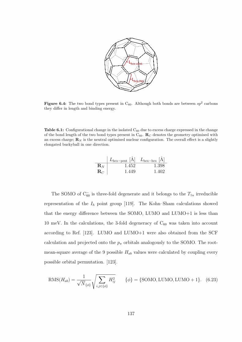
Lhex-pent
Lhex-hex
Figure 6.4: The two bond types present in C60. Although both bonds are between sp2 carbonsthey differ in length and binding energy.
Table 6.1: Configurational change in the isolated C60 due to excess charge expressed in the changeof the bond length of the two bond types present in C60. RC denotes the geometry optimised withan excess charge; RN is the neutral optimised nuclear configuration. The overall effect is a slightlyelongated buckyball in one direction.
Lhex−pent [A] Lhex−hex [A]RN 1.452 1.398RC 1.449 1.402
The SOMO of C−60 is three-fold degenerate and it belongs to the T1u irreducible
representation of the Ih point group [119]. The Kohn–Sham calculations showed
that the energy difference between the SOMO, LUMO and LUMO+1 is less than
10 meV. In the calculations, the 3-fold degeneracy of C60 was taken into account
according to Ref. [123]. LUMO and LUMO+1 were also obtained from the SCF
calculation and projected onto the pπ orbitals analogously to the SOMO. The root-
mean-square average of the 9 possible Hab values were calculated by coupling every
possible orbital permutation. [123].
RMS(Hab) =1√Nφ
√ ∑i,j∈φ
H2ij φ = SOMO,LUMO,LUMO + 1. (6.23)
137

6.4 Results & discussion
In order to assess the Hab probability distribution, a large neighbour distance cut-off
of 15 A was chosen. At 300 K the distributions clearly show the difference between
the second and first nearest neighbours. By integrating the peaks on the probability
distribution plot Fig. 6.5 separately, the first sharp peak gives 0.333 corresponding
to the six second nearest neighbours (at 14.01 A) which were within the cut-off
distance, and the rest gives 0.666 which corresponds to the twelve nearest neighbours.
The average coupling for the nearest neighbours was 〈Hab〉1st = 16.4 meV with a
maximum of max(Hab) = 37.0 meV . The second peak showed an average coupling
of 〈Hab〉2nd = 0.1 meV. The Hab values are so small for the second nearest neighbours
that ignoring them does not affect the mobility values. The peak of the distribution
for nearest neighbours is around 15.07 meV. While the average coupling from AOM
is very close to the values obtained from FODFT by Oberhofer et al. (14 meV) the
maximum value is only half of the maximum value with FODFT (68 meV in Ref
[45]). This is due to the averaging over the degenerate states which was carried out
for the AOM couplings but not for the FODFT couplings. As discussed previously
in Chapters 4 and 5, the relative rotational orientation has a significant role in the
magnitude of the coupling for π-conjugated systems. This is especially true for large
molecules such as C60 which has a complex nodal structure (see Fig. 2.3). Due to this
effect, the 9 possible coupling values are strongly anti-correlated by the orthogonality
of the orbitals. If one orbital pair gives a very high coupling, some of the couplings
due to the inclusion of orthogonal orbitals give a lower coupling, thereby reducing
the mean coupling value. Therefore, the averaging has a very pronounced effect in
evening out the coupling values. As a consequence, the peak representing the nearest
neighbours is rather narrow (Fig. 6.5).
138

Figure 6.5: Distribution of the electronic coupling values for FCC C60 crystal at 300 K fora 1 ns trajectory. The neighbour distance cut-off was 15 A including nearest and second nearestneighbours. The RMS averaging of the coupling values according to Eq. (6.23) resulted in relativelynarrow peaks.
It is interesting to compare the effect of the dynamics on the coupling values as
well. In Fig 6.6, the temperature dependency of the Hab values can be seen along the
different directions. It is known from experiment that crystalline C60 goes through
phase transition at 255 K where the degree of rotational freedom reduces to two
therefore the system is not completely isotropic anymore. This is reflected by the
coupling distribution. At 500 K, the coupling distribution is very similar to the
300 K case: the maximum coupling was 36.4 meV, the mean was 16.63 meV while
the maximum of the distribution was at 15 meV. Meanwhile at 100 K, the effect
of the phase transition becomes obvious: the spread of the coupling values is wider
ranging between 3.8 meV and 47.9 meV and the distribution is not smooth anymore.
More importantly the anisotropy can be visualised by plotting the Hab values along
the lattice directions (Fig 6.6).
139

Figure 6.6: Distribution of the electronic coupling values for FCC C60 crystal at different tem-peratures for a 1 ns trajectory along the three axes for the nearest neighbours only. The 300 Ktrajectory on Panel A shows an isotropic distribution of coupling values while the 100 K trajectoryhas distinct peaks and in the z direction the distribution differs from the almost identical x and ydirections. This is due to the phase transition in the crystalline C60 below 100K which preventsfree rotation of the molecules. Such coupling distribution indicates that while at 300 K the mobilitytensor is expected to be isotropic at 100 K this may not be true.
The inner-sphere contribution of the reorganisation energy λi, according to Eq. (6.5),
was 105.33 meV and the outer-sphere contribution, according to Eq. (6.6), was
around 38 meV. It is important to note that in this approximation the maximum
Hab value is 37 meV which although comparable to the reorganisation energy (143
meV) is less than 3/8 λ therefore the localised transport approximation does not
break down in this case. This is due to the aforementioned smoothing effect of the
RMS averaging. In fact, if the Hab values are compared without averaging it can be
seen that the maximum value goes up to 73 meV while the average value is 13 meV
and the distribution can be approximated with half a Gaussian around 0 (Fig 6.7).
This means that if averaging is not applied some of the coupling values are too high
to assume localisation and the approximation breaks down.
140

Figure 6.7: Distribution of the Hij values in FCC C60 crystal at 300 K for a 100 ps trajectorywhen no RMS averaging is applied to the coupling values. The mean is 13 meV while the maximumcoupling is 73 meV.
Figure 6.8: Distribution of the site energy difference for FCC C60 crystal at 300 K for a 100 pstrajectory. The energy peaks form a Gaussian with a mean of 0 meV and a standard deviation of52.3 meV.
141

The site energy difference between the sites showed a Gaussian distribution with a
mean of 0 and the standard deviation of 52.3 meV (Fig 6.8). The effective frequency
obtained from the spectral density function according to Eq. (6.10) is 1624 cm−1, this
was obtained by using the vertical energy gap obtained for 100 ps long MD trajectory.
The site energy differences are rather large compared to the Hab values and are quite
likely to dominate the Franck–Condon factor if the instantaneous values are used.
This is elaborated in the next section where the different time scales are analysed.
6.4.1 Time scales
It was discussed how the different values on which the rates depend can be calculated.
However, it is worth paying close attention to which values are averaged and which
values are instantaneous in the formula. This can be achieved by comparing the
time scales of the rate, the electronic coupling matrix elements, and the site energy
difference. To this end, the Fourier transforms of the coupling values and ∆Eij are
compared to the distribution of rates in the system.
The Fourier transform of the Hab values reveals that the change in the coupling
values are dominated by low frequency components (Fig. 6.9). This is due to the
importance of relative orientation for molecules with a complex nodal structure such
as C60 therefore the change in coupling values is dominated by the rotation of the
buckyballs.
142

Figure 6.9: Discrete cosine transform of the electronic coupling for a dimer in a FCC C60 crystalat 300 K for a 100 ps trajectory. The spectrum is dominated by slowly changing parameters. Thiscorresponds to our expectations that in the case of C60 the rotation has the most significant effecton the coupling.
Figure 6.10: Discrete cosine transform of the site energy difference for a dimer in a FCC C60
crystal at 300 K for a 100 ps trajectory. The lower peak at 487 cm−1 corresponds to the breathingmode of the C60 cage. The higher frequency term is comparable to the frequency of a carbon doublebond stretch.
143
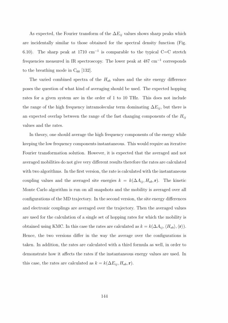
As expected, the Fourier transform of the ∆Eij values shows sharp peaks which
are incidentally similar to those obtained for the spectral density function (Fig.
6.10). The sharp peak at 1710 cm−1 is comparable to the typical C=C stretch
frequencies measured in IR spectroscopy. The lower peak at 487 cm−1 corresponds
to the breathing mode in C60 [132].
The varied combined spectra of the Hab values and the site energy difference
poses the question of what kind of averaging should be used. The expected hopping
rates for a given system are in the order of 1 to 10 THz. This does not include
the range of the high frequency intramolecular term dominating ∆Eij, but there is
an expected overlap between the range of the fast changing components of the Hij
values and the rates.
In theory, one should average the high frequency components of the energy while
keeping the low frequency components instantaneous. This would require an iterative
Fourier transformation solution. However, it is expected that the averaged and not
averaged mobilities do not give very different results therefore the rates are calculated
with two algorithms. In the first version, the rate is calculated with the instantaneous
coupling values and the averaged site energies k = k(∆Aij, Hab, r). The kinetic
Monte Carlo algorithm is run on all snapshots and the mobility is averaged over all
configurations of the MD trajectory. In the second version, the site energy differences
and electronic couplings are averaged over the trajectory. Then the averaged values
are used for the calculation of a single set of hopping rates for which the mobility is
obtained using KMC. In this case the rates are calculated as k = k(∆Aij, 〈Hab〉, 〈r〉).
Hence, the two versions differ in the way the average over the configurations is
taken. In addition, the rates are calculated with a third formula as well, in order to
demonstrate how it affects the rates if the instantaneous energy values are used. In
this case, the rates are calculated as k = k(∆Eij, Hab, r).
144
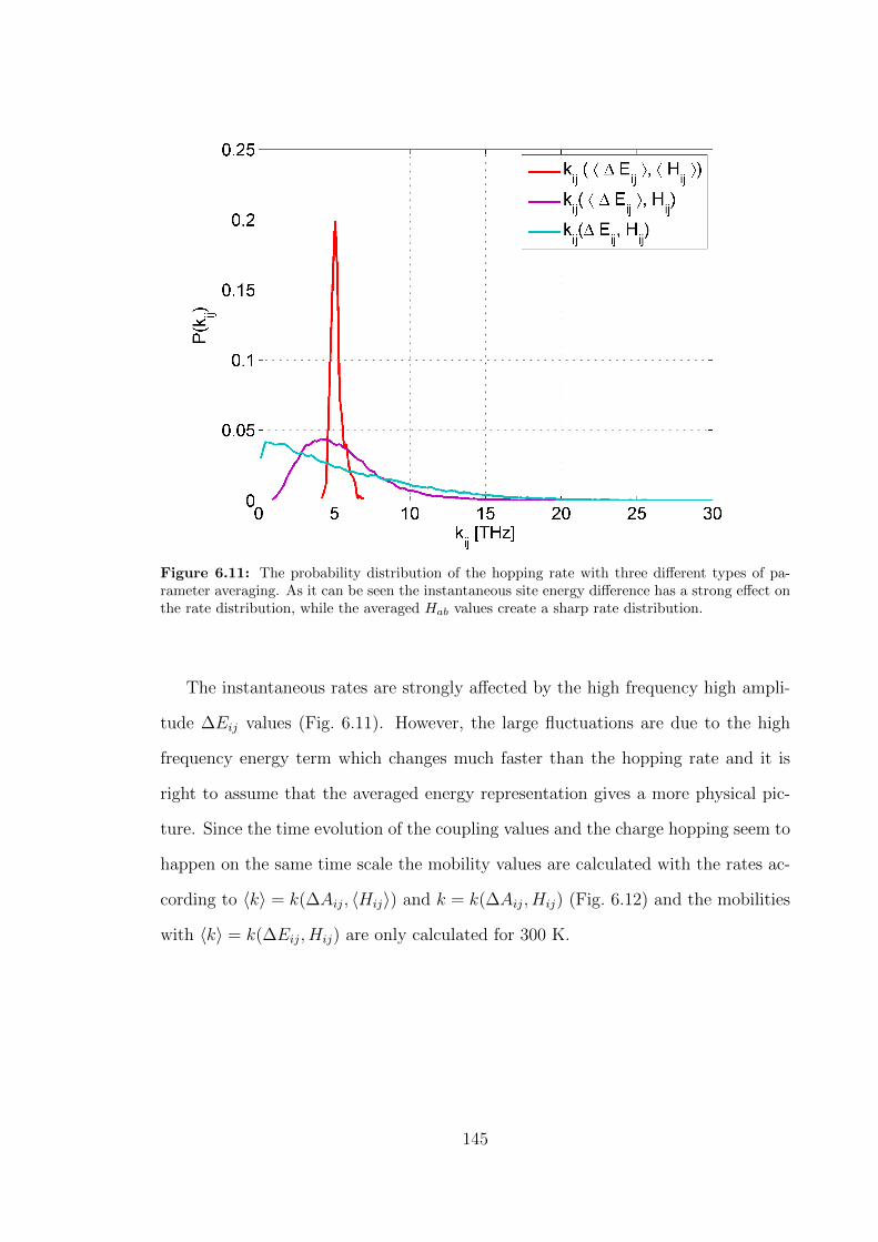
Figure 6.11: The probability distribution of the hopping rate with three different types of pa-rameter averaging. As it can be seen the instantaneous site energy difference has a strong effect onthe rate distribution, while the averaged Hab values create a sharp rate distribution.
The instantaneous rates are strongly affected by the high frequency high ampli-
tude ∆Eij values (Fig. 6.11). However, the large fluctuations are due to the high
frequency energy term which changes much faster than the hopping rate and it is
right to assume that the averaged energy representation gives a more physical pic-
ture. Since the time evolution of the coupling values and the charge hopping seem to
happen on the same time scale the mobility values are calculated with the rates ac-
cording to 〈k〉 = k(∆Aij, 〈Hij〉) and k = k(∆Aij, Hij) (Fig. 6.12) and the mobilities
with 〈k〉 = k(∆Eij, Hij) are only calculated for 300 K.
145

Figure 6.12: The probability distribution of the hopping rate compared to the Fourier transformof the site energy difference and the Fourier transform of the electronic coupling values. It can beseen that rates are in general slower than the site energy difference changes, while the difference isnot so straightforward for the coupling timescales.
The mobility values calculated for the systems can be seen in Tables 6.2 and 6.3.
All eigenvalues of the mobility matrices were the same at high temperatures 300K
and 500K. This is due to the free rotation of the molecules, hence the mobility is
homogeneous. However, at 100 K the phase transition to non-free rotating crystal
becomes obvious from the mobility values where in the z direction the mobility was
less than half of that of x and y. This corresponds to the previously shown Hij
distribution in Fig. 6.6.
146
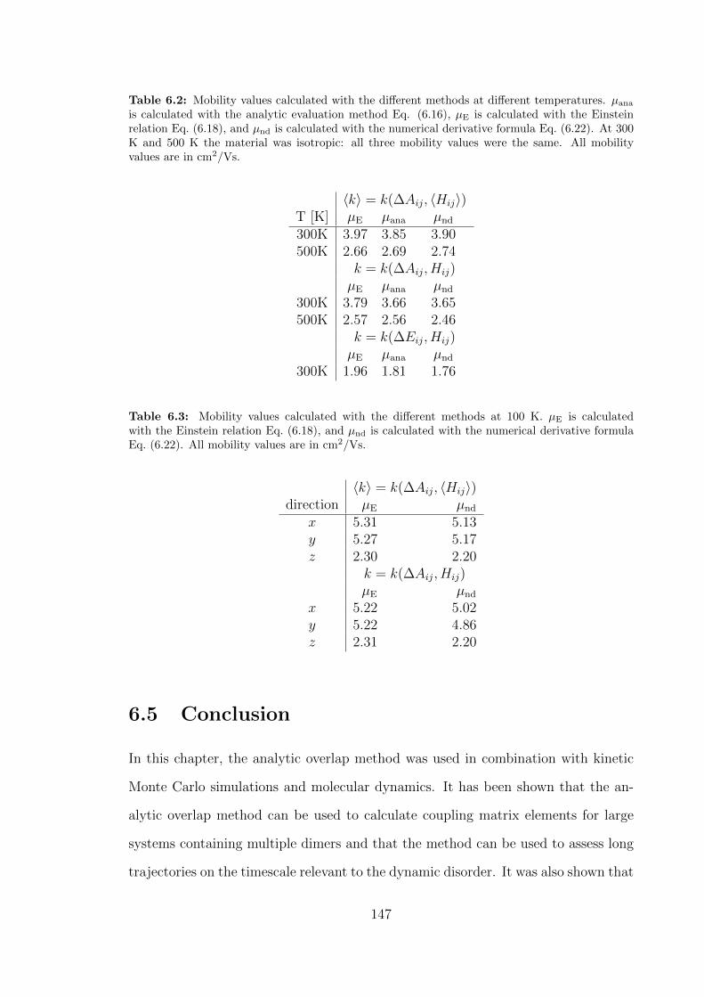
Table 6.2: Mobility values calculated with the different methods at different temperatures. µana
is calculated with the analytic evaluation method Eq. (6.16), µE is calculated with the Einsteinrelation Eq. (6.18), and µnd is calculated with the numerical derivative formula Eq. (6.22). At 300K and 500 K the material was isotropic: all three mobility values were the same. All mobilityvalues are in cm2/Vs.
〈k〉 = k(∆Aij, 〈Hij〉)T [K] µE µana µnd
300K 3.97 3.85 3.90500K 2.66 2.69 2.74
k = k(∆Aij, Hij)µE µana µnd
300K 3.79 3.66 3.65500K 2.57 2.56 2.46
k = k(∆Eij, Hij)µE µana µnd
300K 1.96 1.81 1.76
Table 6.3: Mobility values calculated with the different methods at 100 K. µE is calculatedwith the Einstein relation Eq. (6.18), and µnd is calculated with the numerical derivative formulaEq. (6.22). All mobility values are in cm2/Vs.
〈k〉 = k(∆Aij, 〈Hij〉)direction µE µnd
x 5.31 5.13y 5.27 5.17z 2.30 2.20
k = k(∆Aij, Hij)µE µnd
x 5.22 5.02y 5.22 4.86z 2.31 2.20
6.5 Conclusion
In this chapter, the analytic overlap method was used in combination with kinetic
Monte Carlo simulations and molecular dynamics. It has been shown that the an-
alytic overlap method can be used to calculate coupling matrix elements for large
systems containing multiple dimers and that the method can be used to assess long
trajectories on the timescale relevant to the dynamic disorder. It was also shown that
147
the mean of the electronic coupling values calculated for the molecular dynamics is
very similar to that obtained by Oberhofer et al. using explicit electronic structure
(FODFT) calculations [45] however the results seem to overestimate the experimen-
tal values obtained for FCC C60 of around 0.5(±0.2) cm2/Vs at room temperature
[130]. In this approximation, the maximum of the coupling values remained small
enough compared to the reorganisation energy that there was a finite energy barrier
between the two states. However this is due to the smoothing effect of the averaged
coupling values. Newton et al. recommends the root-mean-square averaging of cou-
plings over degenerate orbitals for coupling values that are relatively similar. This
was not an issue for the hemes in Ref. [79] where the coupling values between the
monomers were similar but the range proved to be much broader in the C60 case. It is
also important that if the averaging is not included, the coupling values occasionally
become so large that the localised transport theory is not valid anymore. Therefore,
C60 systems are better described by other methods where there is no assumptions of
charge localisation and the degeneracy is included differently. For example, in the
case of non-adiabatic molecular dynamics the degenerate states are part of the basis
set of localised diabatic states. Using surface hopping on such a system would show
that the charge does not remain on a single site but spreads over multiple sites and
instead of discrete hops the excess charge would propagate in the system as a wave
packet while the nuclear configuration switches from one potential energy surface to
the other.
Nevertheless, the KMC study of the averaged coupling gives a good illustrative
example of the importance of the dynamic effects and how they should be included
in the rate calculation. Furthermore, the dynamic effects also gave an interesting
example of how the temperature affects the isotropy of the mobility which gives an
interesting tool to study other systems with different dynamic characteristics such
as pentacene and rubrene.
148
7 Conclusion & Outlook
7.1 Conclusion
This work presented some of the main challenges of modelling charge transport in
organic semiconductors. In Chapter 3, the most widely used models for discussing
charge transport in organic semiconductors were presented including their shortcom-
ings in assuming completely localised or delocalised charge carrier states. Then, two
other models were shown which provide a more generic but computationally more
intensive solution requiring the accurate and efficient calculation of the electronic
coupling matrix elements, the overlap matrix, and the non-adiabatic coupling vector
elements. The main focus of this work was to obtain these values to support charge
transport modelling in organic semiconductors.
In order to understand the accuracy of the different methods in Chapter 4, vari-
ous coupling calculation methods were compared for seven π-conjugated negatively
charged molecules. The couplings were calculated between perfectly stacked dimers
at different separation length. Another set was constructed with randomly oriented
anthracene molecules. The reference calculations were performed using a high level
ab initio SCS-CC2 method in combination with generalised Mulliken–Hush theory.
Then the couplings were calculated with charge constrained density functional theory
with different exchange correlation functionals, fragment orbital DFT, and fragment
orbital density functional tight-binding. Of these methods, CDFT with 50% exact
exchange had the smallest relative error compared to the reference values. Decreas-
ing the proportion of exact exchange increased the errors significantly. Slightly faster
than CDFT+PBE, FODFT+PBE also matched the reference values better as over-
149

delocalisation was prevented by the separation of dimers. HSE06 functional yielded
very similar results to CDFT/25 (PBE0) therefore, there was no clear advantage of
using range separated functional for these systems. FODFT results also had similar
errors to CDFT/25. Although FODFTB was the fastest method, the errors were
rather large compared to the reference values which is due to the limitations of the
minimum basis set applied for these simulations. The relative error improved with
all methods when a linear scaling factor was applied to the results. The results also
showed that the methods are less accurate for the randomly oriented anthracenes
than for the stacked system. This is due to the complicated nodal system of an-
thracene molecules.
Since CDFT with 50% exact exchange proved to be the best approach for both
reduced and oxidised example molecules [68] it is expected to be transferable to other
π-conjugated systems. Of the methods presented here only FODFTB is fast enough
to be used in combination with non-adiabatic molecular dynamics but the errors are
comparatively large which can cause issues in systems where the couplings fluctuate
around values which suggest localised or delocalised transport. This motivated the
development of an alternative method which not only provides the coupling matrix
elements but also the overlap and the non-adiabatic coupling vectors.
The ultrafast and accurate semi-empirical analytic overlap method approximates
the intermolecular electronic coupling between π-conjugated organic molecules as
a linear function of the overlap between the SOMO of the donor and acceptor
molecules. The approximation was tested in the range relevant to electron transport
in the condensed phase (5 to 500 meV). It was also shown that a single propor-
tionality constant is suitable to describe a broad set of molecules including arenes
with heteroatoms, acenes and fullerenes. The accuracy also holds if the basis set is
replaced with the minimum STO basis set with optimised Slater decay coefficients.
Furthermore, the analytic overlap method can be used to evaluate coupling values
for rate equation based transport models. This was demonstrated on a set of heme
150

dimers. Here, the effect of molecular dynamics was also taken into account. In order
to reduce computational demand, the contribution of the d-orbitals to the overlap
values was neglected. The issue partly arose from the magnitude of the Hab values
as many of them were below the accuracy of 0.5 meV which was achievable with
FODFT for these degenerate systems. More importantly, the issues came from the
large fluctuations of the heme structures during molecular dynamics. In its current
form, this model may not be best suited for charge transport modelling in biological
systems where small couplings act as a bottleneck for the process.
The analytic overlap method can also be used to approximate the non-adiabatic
coupling vector elements for π-conjugated systems. The method was benchmarked
with FODFT on an ethylene dimer which showed that the NACV components point-
ing from one molecule to the other could be reproduced well with the AOM. Although
the results were less accurate along the bonds, this is unlikely to cause issues as the
nuclear forces arising from the off-diagonals of the Hamiltonian are two orders of
magnitude smaller than the nuclear forces in the same direction. It is also expected
that the absolute errors are smaller for any other π-conjugated system since the
NACV elements are smaller in more extended systems.
The main benefit of the developed program is that it allows for an ultrafast
estimation of off-diagonal elements. In fact, the speed-up with respect to DFT
calculations is six orders of magnitude while the loss in accuracy compared to the
benchmark values is within chemical accuracy. These results are very encouraging
and set the stage for non-adiabatic molecular dynamics simulation of charge transfer
in future work.
The analytic overlap method was also used in combination with kinetic Monte
Carlo simulations and molecular dynamics. It was demonstrated that the analytic
overlap method can be used to calculate coupling matrix elements for large systems
containing multiple dimers and that the method can be used to assess long trajec-
tories on the timescale relevant to the dynamic disorder in organic semiconductors.
151
In this approximation, the maximum of the coupling values remained small enough
compared to the reorganisation energy that there was a finite energy barrier between
the two states. However, this is due to the smoothing effect of the averaged coupling
values. It is worth noting here that when the averaging is omitted, the AOM cou-
plings obtained for the molecular dynamics trajectories give very similar statistics
to the one reported by Oberhofer et al. using idealised C60 molecules and FODFT
in Ref. [45]. This is in stark contrast with the heme values where the correlation
between FODFT and AOM was poor. This is due to the fact that C60 is much more
rigid than a heme and the idealised coefficients give a better approximation for the
coupling values. As these non-averaged Hab values are not all compatible with small
polaron hopping theory, it is expected that non-adiabatic molecular dynamics gives
better results for C60 mobilities as it does not assume charge localisation and the
degeneracy is included differently. Nevertheless, the KMC study of the averaged
coupling serves as an example of the importance of the dynamic effects in organic
semiconductors and how the time scales of the hopping rate, the coupling values,
and the energy difference affects the mobility. Furthermore, it was also discussed
how the temperature affects the isotropy of the mobility, which makes it worthwhile
to compare analysis done on other systems such as PCBM to C60 results.
7.2 Outlook
Based on the findings of this project there are a number of avenues of further re-
search that can be explored. The series of benchmark calculations discussed charge
transport with different methods in the reduced state. A follow-up project has been
proposed which assesses donor-bridge-acceptor systems in order to better understand
how well different methods can predict mediated charge transport. The first project
of the series tackles small non-biological systems, with the eventual aim of building
on this to understand the effects in biological systems such as amino acids and DNA
152

base pairs [109].
The analytic overlap and the non-adiabatic coupling vector calculation code was
built partly to support non-adiabatic MD and the first results on a chain of ethylene
molecules can be seen in the work of Spencer et al. [133]. The same method can
be applied to actual organic semiconductor systems such as rubrene and pentacene.
It was briefly mentioned in the conclusion section that in its current form the ana-
lytic overlap method is not suitable for analysing less rigid molecules such as heme
cofactors. However, it is possible to adapt the code by defining a number of coeffi-
cient sets obtained for different molecular dynamics snapshots of hemes which form
a sample coefficient set. Couplings of an independent molecular dynamics trajectory
may be calculated by fitting the molecules to this set by minimising the root-mean-
square deviation of the molecules and finding the most appropriate coefficient set to
describe the given heme.
Even though the AOM model in its current form is useful for systems with large
coupling values, the calculation of small coupling values below 5 meV remains a
challenge. This was not unique to the AOM and similar trends were observed when
other methods were compared to generalised Mulliken–Hush theory results. We
found that with the AOM method the results can be improved for carbon atom and
C60 results if different Slater coefficients are used for different p integrals depending
on whether the alignment is π-type or σ-type, but the transferability of this approach
was not tested. In order to be able to efficiently use the model in biological systems,
the error value for small couplings has to be reduced. Furthermore, timeliness of the
code can be improved further by parallelising the code.
The methods presented here are approximate and it would be very interesting
to compare the non-adiabatic dynamics results with the work of Martinez et al who
used shared memory CPU/GPU architecture to gain significant speed-up for TDDFT
and DFT calculation and simulated non-adiabatic dynamics in a multiheme system
[134].
153

Finally, it would also be interesting to compare the KMC results obtained for
C60 with other non-free rotating molecules and how the different dynamic properties
affect the time scales of the energy and the coupling values, as well as the isotropy.
154

Bibliography
[1] Mihai Irimia-Vladu. ”Green”electronics: biodegradable and biocompatible ma-
terials and devices for sustainable future. Chemical Society Reviews, 43(2):588–
610, 2014.
[2] Gerwin H Gelinck, H Edzer a Huitema, Erik van Veenendaal, Eugenio Can-
tatore, Laurens Schrijnemakers, Jan B P H van der Putten, Tom C T Geuns,
Monique Beenhakkers, Jacobus B Giesbers, Bart-Hendrik Huisman, Eduard J
Meijer, Estrella Mena Benito, Fred J Touwslager, Albert W Marsman, Bas
J E van Rens, and Dago M de Leeuw. Flexible active-matrix displays and shift
registers based on solution-processed organic transistors. Nature materials,
3(2):106–10, 2004.
[3] K Myny, S Steudel, S Smout, P Vicca, F Furthner, B. Van Der Putten, A. K.
Tripathi, G. H. Gelinck, J Genoe, W. Dehaene, and P Heremans. Organic
RFID transponder chip with data rate compatible with electronic product
coding. Organic Electronics: physics, materials, applications, 11(7):1176–1179,
2010.
[4] M. Slawinski, M. Weingarten, M. Heuken, A. Vescan, and H. Kalisch. Inves-
tigation of large-area OLED devices with various grid geometries. Organic
Electronics: physics, materials, applications, 14(10):2387–2391, 2013.
[5] Minze T. Rispens, Auke Meetsma, Roman Rittberger, Christoph J. Brabec,
N. Serdar Sariciftci, and Jan C. Hummelen. Influence of the solvent on the
crystal structure of PCBM. Chemical Communications, (17):2116, August
2003.
[6] A. Shah, J. Meier, A. Buechel, U. Kroll, J. Steinhauser, F. Meillaud, H. Schade,
and D. Domine. Towards very low-cost mass production of thin-film silicon
155
photovoltaic (PV) solar modules on glass. In Thin Solid Films, volume 502,
pages 292–299, 2006.
[7] Giuseppe Paterno, Anna J. Warren, Jacob Spencer, Gwyndaf Evans, Victo-
ria Garcıa Sakai, Jochen Blumberger, and Franco Cacialli. Micro-focused X-
ray diffraction characterization of high-quality [6,6]-phenyl-C61-butyric acid
methyl ester single crystals without solvent impurities. Journal of Materials
Chemistry C, 1(36):5619, August 2013.
[8] Mengmeng Li, Cunbin An, Wojciech Pisula, and Klaus Mullen. Align-
ment of organic semiconductor microstripes by two-phase dip-coating. Small,
10(10):1926–1931, 2014.
[9] Nihat Tugluoglu, Behzad Baris, Hatice Gurel, Serdar Karadeniz, and
Omer Faruk Yuksel. Investigation of optical band gap and device parame-
ters of rubrene thin film prepared using spin coating technique. Journal of
Alloys and Compounds, 582:696–702, 2014.
[10] Anke Teichler, Jolke Perelaer, and Ulrich S. Schubert. Inkjet printing of or-
ganic electronics – comparison of deposition techniques and state-of-the-art
developments. Journal of Materials Chemistry C, 1(10):1910, 2013.
[11] Jean-Luc Bredas, Joseph E Norton, Jerome Cornil, and Veaceslav Coropceanu.
Molecular understanding of organic solar cells: the challenges. Accounts of
chemical research, 42(11):1691–9, November 2009.
[12] Bernard Kippelen and Jean-Luc Bredas. Organic photovoltaics. Energy &
Environmental Science, 2(3):251, March 2009.
[13] Yongbo Yuan, Gaurav Giri, Alexander L. Ayzner, Arjan P. Zoombelt, Stefan
C. B. Mannsfeld, Jihua Chen, Dennis Nordlund, Michael F. Toney, Jinsong
Huang, and Zhenan Bao. Ultra-high mobility transparent organic thin film
156

transistors grown by an off-centre spin-coating method. Nature communica-
tions, 5:3005, January 2014.
[14] Nichole C. Cates, Roman Gysel, Zach Beiley, Chad E. Miller, Michael F. Toney,
Martin Heeney, Lain McCulloch, and Michael D. McGehee. Tuning the prop-
erties of polymer bulk heterojunction solar cells by adjusting fullerene size to
control intercalation. Nano Letters, 9(12):4153–4157, December 2009.
[15] Minh Trung Dang, Guillaume Wantz, Habiba Bejbouji, Mathieu Urien,
Olivier J. Dautel, Laurence Vignau, and Lionel Hirsch. Polymeric solar cells
based on P3HT:PCBM: Role of the casting solvent. Solar Energy Materials
and Solar Cells, 95(12):3408–3418, 2011.
[16] Y N Li, Prashant Sonar, Leanne Murphy, and Wei Hong. High mobility
diketopyrrolopyrrole (DPP)-based organic semiconductor materials for organic
thin film transistors and photovoltaics. Energy & Environmental Science,
6(6):1684–1710, 2013.
[17] Wei Xie, Kathryn A. McGarry, Feilong Liu, Yanfei Wu, P. Paul Ruden,
Christopher J. Douglas, and C. Daniel Frisbie. High-mobility transistors based
on single crystals of isotopically substituted rubrene-d28. Journal of Physical
Chemistry C, 117(22):11522–11529, June 2013.
[18] Ke Zhou, Huanli Dong, Hao-Li Zhang, and Wenping Hu. High performance
n-type and ambipolar small organic semiconductors for organic thin film tran-
sistors. Physical Chemistry Chemical Physics, 16(41):22448–57, 2014.
[19] Tao Liu and Alessandro Troisi. Understanding the Microscopic Origin of the
Very High Charge Mobility in PBTTT: Tolerance of Thermal Disorder. Ad-
vanced Functional Materials, 24(7):925–933, September 2013.
[20] Jui-Fen Chang, Tomo Sakanoue, Yoann Olivier, Takafumi Uemura, Marie-
Beatrice Dufourg-Madec, Stephen G. Yeates, Jerome Cornil, Jun Takeya,
157
Alessandro Troisi, and Henning Sirringhaus. Hall-Effect Measurements Prob-
ing the Degree of Charge-Carrier Delocalization in Solution-Processed Crys-
talline Molecular Semiconductors. Physical Review Letters, 107(6):066601, Au-
gust 2011.
[21] Paul A. Heiney. Structure, dynamics and ordering transition of solid C60.
Journal of Physics and Chemistry of Solids, 53(11):1333–1352, 1992.
[22] Thorsten Vehoff, Alessandro Troisi, and Denis Andrienko. Charge Transport
in Organic Crystals : Role of Disorder and Topological Connectivity. Journal
of Physical Chemistry C, 118(8):11702–11708, 2010.
[23] Tao Liu and Alessandro Troisi. What makes fullerene acceptors special as
electron acceptors in organic solar cells and how to replace them. Advanced
Materials, 25(7):1038–1041, February 2013.
[24] C.W. Chang, B.C. Regan, W. Mickelson, R.O. Ritchie, and A. Zettl. Probing
structural phase transitions of crystalline C60 via resistivity measurements of
metal film overlayers. Solid State Communications, 128(9-10):359–363, De-
cember 2003.
[25] Lidong Zheng and Yanchun Han. Solvated crystals based on [6,6]-phenyl-C61-
butyric acid methyl ester (PCBM) with the hexagonal structure and their
phase transformation. Journal of Physical Chemistry B, 116(5):1598–1604,
February 2012.
[26] Alessandro Troisi. Charge transport in high mobility molecular semiconduc-
tors: classical models and new theories. Chemical Society reviews, 40(5):2347–
58, May 2011.
[27] V. Podzorov, E. Menard, J. a. Rogers, and M. E. Gershenson. Hall effect in
the accumulation layers on the surface of organic semiconductors. Physical
Review Letters, 95(22):226601, November 2005.
158
[28] Kazuhiro Marumoto, Shin Ichi Kuroda, Taishi Takenobu, and Yoshihiro Iwasa.
Spatial extent of wave functions of gate-induced hole carriers in pentacene
field-effect devices as investigated by electron spin resonance. Physical Review
Letters, 97(25):256603, December 2006.
[29] S. Fratini and S. Ciuchi. Bandlike motion and mobility saturation in organic
molecular semiconductors. Physical Review Letters, 103(26):266601, December
2009.
[30] Joe J. Kwiatkowski, Jarvist M. Frost, and Jenny Nelson. The effect of mor-
phology on electron field-effect mobility in disordered C60 thin films. Nano
Letters, 9(3):1085–1090, 2009.
[31] Rocco P Fornari and Alessandro Troisi. Theory of charge hopping along a
disordered polymer chain. Physical Chemistry Chemical Physics, 16(21):9997–
10007, January 2014.
[32] T Holstein. Studies of polaron motion. Annals of Physics, 8(3):325–342,
November 1959.
[33] Alessandro Troisi. Quantum dynamic localization in the Holstein Hamiltonian
at finite temperatures. Physical Review B - Condensed Matter and Materials
Physics, 82(24):245202, December 2010.
[34] Roel S. Sanchez-Carrera, Pavel Paramonov, Graeme M. Day, Veaceslav
Coropceanu, and Jean Luc Bredas. Interaction of charge carriers with lat-
tice vibrations in oligoacene crystals from naphthalene to pentacene. Journal
of the American Chemical Society, 132(41):14437–14446, October 2010.
[35] Henning Sirringhaus, Tomo Sakanoue, and Jui Fen Chang. Charge-transport
physics of high-mobility molecular semiconductors. Physica Status Solidi (B)
Basic Research, 249(9):1655–1676, 2012.
159
[36] Veaceslav Coropceanu, Jerome Cornil, Demetrio a. da Silva Filho, Yoann
Olivier, Robert Silbey, and Jean Luc Bredas. Charge transport in organic
semiconductors. Chemical Reviews, 107(4):926–952, April 2007.
[37] Charles Kittel. Introduction to solid state physics. John Wiley & Sons, 7
edition, 2005.
[38] Neil W Ashcroft and N David Mermin. Solid State Physics, volume 2. Harcourt
College Publisher, 1976.
[39] N. Karl. Charge carrier transport in organic semiconductors. In Synthetic
Metals, volume 133-134, pages 649–657, 2003.
[40] Tomo Sakanoue and Henning Sirringhaus. Band-like temperature dependence
of mobility in a solution-processed organic semiconductor. Nature materials,
9(9):736–40, September 2010.
[41] Jochen Blumberger. Recent Advances in the Theory and Molecular Simulation
of Biological Electron Transfer Reactions. Chemical Reviews, 115(20):11191–
11238, October 2015.
[42] R. A. Marcus. On the Theory of Oxidation-Reduction Reactions Involving
Electron Transfer. I. The Journal of Chemical Physics, 24(5):966, December
1956.
[43] T. Holstein. Studies of Polaron Motion Part II. The ”Small” Polaron. Annals
of Physics, 281(1-2):725–773, April 2000.
[44] Abraham Nitzan. Chemical Dynamics in Condensed Phases: Relaxation,
Transfer, and Reactions in Condensed Molecular Systems (Oxford Graduate
Texts), volume 8. Oxford University Press, 2006.
[45] Harald Oberhofer and Jochen Blumberger. Revisiting electronic couplings and
incoherent hopping models for electron transport in crystalline C60 at ambient
160

temperatures. Physical Chemistry Chemical Physics, 14(40):13846, October
2012.
[46] Jenny Nelson, Joe J. Kwiatkowski, James Kirkpatrick, and Jarvist M. Frost.
Modeling charge transport in organic photovoltaic materials. Accounts of
Chemical Research, 42(11):1768–1778, 2009.
[47] Alessandro Troisi. The speed limit for sequential charge hopping in molecular
materials. Organic Electronics: physics, materials, applications, 12(12):1988–
1991, December 2011.
[48] David L. Cheung and Alessandro Troisi. Theoretical study of the organic
photovoltaic electron acceptor PCBM : morphology, electronic structure, and
charge localization. The Journal of Physical Chemistry C, 114(48):20479–
20488, December 2010.
[49] Fruzsina Gajdos, Harald Oberhofer, Michel Dupuis, and Jochen Blumberger.
On the inapplicability of electron-hopping models for the organic semicon-
ductor phenyl-C61-butyric acid methyl ester (PCBM). Journal of Physical
Chemistry Letters, 4(6):1012–1017, March 2013.
[50] Lionel Friedman. Electron-phonon interaction in organic molecular crystals.
Physical Review, 140(5A), 1965.
[51] K. Hannewald, V. M. Stojanovic, J. M. T. Schellekens, P. a. Bobbert,
G. Kresse, and J. Hafner. Theory of polaron bandwidth narrowing in organic
molecular crystals. Physical Review B, 69(7):075211, February 2004.
[52] E. Mozafari and S. Stafstrom. Polaron dynamics in a two-dimensional Holstein-
Peierls system. Journal of Chemical Physics, 138(18):0–7, 2013.
[53] John C. Tully. Mixed quantum-classical dynamics. Faraday Discussions,
110(0):407–419, January 1998.
161

[54] Priya V. Parandekar and John C. Tully. Mixed quantum-classical equilibrium.
Journal of Chemical Physics, 122(9):094102, March 2005.
[55] Linjun Wang and David Beljonne. Flexible surface hopping approach to model
the crossover from hopping to band-like transport in organic crystals. Journal
of Physical Chemistry Letters, 4(11):1888–1894, June 2013.
[56] Adam Kubas, Fruzsina Gajdos, Alexander Heck, Harald Oberhofer, Marcus
Elstner, and Jochen Blumberger. Electronic couplings for molecular charge
transfer: benchmarking CDFT, FODFT and FODFTB against high-level ab
initio calculations. II. Physical Chemistry Chemical Physics, 17(22):14342–
14354, 2015.
[57] Seth Difley and Troy Van Voorhis. Exciton/charge-transfer electronic couplings
in organic semiconductors. Journal of Chemical Theory and Computation,
7(3):594–601, 2011.
[58] Troy Van Voorhis, Tim Kowalczyk, Benjamin Kaduk, Lee-Ping Wang, Chiao-
Lun Cheng, and Qin Wu. The diabatic picture of electron transfer, reaction
barriers, and molecular dynamics. Annual review of physical chemistry, 61:149–
70, January 2010.
[59] Robert S. Mulliken. Molecular compounds and their spectra. II. Journal of
the American Chemical Society, 74(8):811–824, 1952.
[60] Noel S. Hush. Intervalence-Transfer Absorption. Theoretical Considerations
and Spectroscopic Data. Progress in Inorganic Chemistry, 8:391–444, 1967.
[61] Noel S. Hush. Homogeneous and heterogeneous optical and thermal electron
transfer. Electrochimica Acta, 13(5):1005–1023, 1968.
[62] Carol Creutz, Marshall D. Newton, and Norman Sutin. Metal-lingad and
162
metal-metal coupling elements. Journal of Photochemistry and Photobiology,
A: Chemistry, 82(1-3):47–59, 1994.
[63] R. J. Cave and M. D. Newton. Generalization of the Mulliken-Hush treatment
for the calculation of electron transfer matrix elements. Chemical Physics
Letters, 249(1-2):15–19, January 1996.
[64] Robert J. Cave and Marshall D. Newton. Calculation of electronic coupling
matrix elements for ground and excited state electron transfer reactions: Com-
parison of the generalized Mulliken–Hush and block diagonalization methods.
The Journal of Chemical Physics, 106(22):9213, 1997.
[65] Peter G. Szalay, Thomas Muller, Gergely Gidofalvi, Hans Lischka, and Ron
Shepard. Multiconfiguration self-consistent field and multireference configura-
tion interaction methods and applications. Chemical Reviews, 112(1):108–181,
January 2012.
[66] C. Angeli, R. Cimiraglia, S. Evangelisti, T. Leininger, and J. P. Malrieu. In-
troduction of n-electron valence states for multireference perturbation theory.
Journal of Chemical Physics, 114(23):10252, 2001.
[67] Celestino Angeli, Renzo Cimiraglia, and Jean Paul Malrieu. n-electron valence
state perturbation theory: A spinless formulation and an efficient implementa-
tion of the strongly contracted and of the partially contracted variants. Journal
of Chemical Physics, 117(20):9138–9153, 2002.
[68] Adam Kubas, Felix Hoffmann, Alexander Heck, Harald Oberhofer, Marcus
Elstner, and Jochen Blumberger. Electronic couplings for molecular charge
transfer: Benchmarking CDFT, FODFT, and FODFTB against high-level ab
initio calculations. Journal of Chemical Physics, 140(10):1–46, December 2014.
[69] Joseph E. Subotnik, Sina Yeganeh, Robert J. Cave, and Mark a. Ratner.
Constructing diabatic states from adiabatic states: Extending generalized
163
Mulliken-Hush to multiple charge centers with Boys localization. Journal of
Chemical Physics, 129(24):244101, December 2008.
[70] Jieru Zheng, Youn K Kang, Michael J Therien, and David N Beratan. Gener-
alized Mulliken-Hush analysis of electronic coupling interactions in compressed
pi-stacked porphyrin-bridge-quinone systems. Journal of the American Chem-
ical Society, 127(32):11303–11310, August 2005.
[71] Christoph Lambert, Gilbert Noll, and Jurgen Schelter. Bridge-mediated hop-
ping or superexchange electron-transfer processes in bis(triarylamine) systems.
Nature materials, 1(1):69–73, September 2002.
[72] Qin Wu and Troy Van Voorhis. Extracting electron transfer coupling ele-
ments from constrained density functional theory. Journal of Chemical Physics,
125(16):164105, October 2006.
[73] F. L. Hirshfeld. Bonded-atom fragments for describing molecular charge den-
sities. Theoretica Chimica Acta, 44(2):129–138, 1977.
[74] Harald Oberhofer and Jochen Blumberger. Electronic coupling matrix elements
from charge constrained density functional theory calculations using a plane
wave basis set. Journal of Chemical Physics, 133(24):244105, December 2010.
[75] Jan Rezac, Bernard Levy, Isabelle Demachy, and Aurelien De La Lande. Ro-
bust and efficient constrained DFT molecular dynamics approach for biochem-
ical modeling. Journal of Chemical Theory and Computation, 8(2):418–427,
2012.
[76] Keith P. McKenna and Jochen Blumberger. Crossover from incoherent to
coherent electron tunneling between defects in MgO. Physical Review B,
86(24):245110, December 2012.
164
[77] Jochen Blumberger and Keith P. McKenna. Constrained density functional
theory applied to electron tunnelling between defects in MgO. Physical Chem-
istry Chemical Physics, 15(1):2184–96, 2013.
[78] Harald Oberhofer and Jochen Blumberger. Insight into the mechanism of the
ru2+-ru3+ electron self-exchange reaction from quantitative rate calculations.
Angewandte Chemie - International Edition, 49(21):3631–3634, May 2010.
[79] Marian Breuer, Kevin M Rosso, and Jochen Blumberger. Electron flow in
multiheme bacterial cytochromes is a balancing act between heme electronic
interaction and redox potentials. Proceedings of the National Academy of Sci-
ences of the United States of America, 111(2):611–6, January 2014.
[80] Marian Breuer, Kevin M. Rosso, and Jochen Blumberger. Flavin Binding
to the Deca-heme Cytochrome MtrC: Insights from Computational Molecular
Simulation. Biophysical Journal, 109(12):2614–2624, December 2015.
[81] M. Elstner, D. Porezag, G. Jungnickel, J. Elsner, M. Haugk, Th. Frauenheim,
S. Suhai, and G. Seifert. Self-consistent-charge density-functional tight-binding
method for simulations of complex materials properties. Physical Review B,
58(11):7260–7268, September 1998.
[82] Michael Gaus, Qiang Cui, and Marcus Elstner. DFTB3: Extension of the
self-consistent-charge density-functional tight-binding method (SCC-DFTB).
Journal of Chemical Theory and Computation, 7(4):931–948, April 2011.
[83] Pekka Koskinen and Ville Makinen. Density-functional tight-binding for be-
ginners. Computational Materials Science, 47(1):237–253, 2009.
[84] Michael Gaus, Albrecht Goez, and Marcus Elstner. Parametrization and
benchmark of DFTB3 for organic molecules. Journal of Chemical Theory and
Computation, 9(1):338–354, January 2013.
165
[85] Tomas Kubar, P Benjamin Woiczikowski, Gianaurelio Cuniberti, and Marcus
Elstner. Efficient calculation of charge-transfer matrix elements for hole trans-
fer in DNA. Journal of Physical Chemistry B, 112(26):7937–47, July 2008.
[86] Alexander Heck, Paul Benjamin Woiczikowski, Tomas Kubar, Kai Welke,
Thomas Niehaus, Bernd Giese, Spiros Skourtis, Marcus Elstner, and
Thomas B. Steinbrecher. Fragment orbital based description of charge trans-
fer in peptides including backbone orbitals. Journal of Physical Chemistry B,
118(16):4261–4272, 2014.
[87] Mario Wolter, Marcus Elstner, and Tomas Kubar. Charge transport in desol-
vated DNA. Journal of Chemical Physics, 139(12), 2013.
[88] Paul Benjamin Woiczikowski, Thomas Steinbrecher, Tomas Kubar, and Mar-
cus Elstner. Nonadiabatic QM/MM simulations of fast charge transfer in Es-
cherichia coli DNA photolyase. Journal of Physical Chemistry B, 115(32):9846–
9863, 2011.
[89] John P. Perdew, Kieron Burke, and Matthias Ernzerhof. Generalized Gradi-
ent Approximation Made Simple. Physical Review Letters, 77(18):3865–3868,
October 1996.
[90] D E Woon and T H Dunning. Gaussian-Basis Sets for Use in Correlated
Molecular Calculations III. the Atoms Aluminum Through Argon. Journal of
Chemical Physics, 98(2):1358–1371, 1993.
[91] Timothy J. Lee and Peter R. Taylor. A diagnostic for determining the qual-
ity of single-reference electron correlation methods. International Journal of
Quantum Chemistry, 36(S23):199–207, June 2009.
[92] John P. Perdew. Density-functional approximation for the correlation energy
of the inhomogeneous electron gas. Physical Review B, 33(12):8822–8824, 1986.
166

[93] A. D. Becke. Density-functional exchange-energy approximation with correct
asymptotic behavior. Physical Review A, 38(6):3098–3100, 1988.
[94] K Eichkorn, F Weigend, O Treutler, and Reinhart Ahlrichs. Auxiliary basis
sets for main row atoms and transition metals and their use to approximate
Coulomb potentials. Theoretical Chemistry Accounts, 97(1-4):119–124, 1997.
[95] Florian Weigend and Reinhart Ahlrichs. Balanced basis sets of split valence,
triple zeta valence and quadruple zeta valence quality for H to Rn: Design and
assessment of accuracy. Physical Chemistry Chemical Physics, 7(18):3297–305,
2005.
[96] Karin Eichkorn, Oliver Treutler, Holger Ohm, Marco Haser, and Reinhart
Ahlrichs. Auxiliary basis sets to approximate Coulomb potentials. Chemical
Physics Letters, 240(4):283–289, 1995.
[97] Marek Sierka, Annika Hogekamp, and Reinhart Ahlrichs. Fast evaluation of the
Coulomb potential for electron densities using multipole accelerated resolution
of identity approximation. Journal of Chemical Physics, 118(20):9136–9148,
2003.
[98] R Ahlrichs, S Backer, M Ehrig, K Eichkorn, S Elliott, F Haase, M Hoser,
H Horn, C Huber, U Huniar, M Kattannek, C Kolmel, M Kollwitz, C Ochsen-
feld, H Ohm, A Schafer, U Schneider, O Treutler, M von Arnim, F Weigend,
P Weis, and H Weiss. TURBOMOLE V6.2 2010, a development of University
of Karlsruhe and Forschungszentrum Karlsruhe GmbH, 1989-2007, TURBO-
MOLE GmbH, since 2007; available from http://www.turbomole.com., 2008.
[99] Ove Christiansen, Henrik Koch, and Poul Jorgensen. The second-order ap-
proximate coupled cluster singles and doubles model CC2. Chemical Physics
Letters, 243(5-6):409–418, 1995.
167

[100] Arnim Hellweg, Sarah a Grun, and Christof Hattig. Benchmarking the per-
formance of spin-component scaled CC2 in ground and electronically excited
states. Physical Chemistry Chemical Physics, 10(28):4119–4127, 2008.
[101] Jonathan C. Rienstra-Kiracofe, Wesley D. Allen, and Henry F. Schaefer.
C2H5+O2 reaction mechanism: High-level ab initio characterizations. Journal
of Physical Chemistry A, 104(44):9823–9840, 2000.
[102] Stefan Grimme. Improved second-order Møller-Plesset perturbation theory
by separate scaling of parallel- and antiparallel-spin pair correlation energies.
Journal of Chemical Physics, 118(20):9095–9102, 2003.
[103] Florian Weigend, Andreas Kohn, and Christof Hattig. Efficient use of the
correlation consistent basis sets in resolution of the identity MP2 calculations.
Journal of Chemical Physics, 116(8):3175–3183, 2002.
[104] Thom H Dunning Jr. Gaussian basis sets for use in correlated molecular calcu-
lations. I. The atoms boron through neon and hydrogen. Journal of Chemical
Physics, 90(1989):1007, 1989.
[105] Jurg Hutter and Marcella Iannuzzi. CPMD: Car-parrinello molecular dynam-
ics. Zeitschrift fur Kristallographie, 220(5-6):549–551, 2005.
[106] N. Troullier and Jose Luriaas Martins. Efficient pseudopotentials for plane-
wave calculations. II. Operators for fast iterative diagonalization. Physical
Review B, 43(11):8861–8869, 1991.
[107] Mark E Tuckerman and Glenn J Martyna. Understanding Modern Molecular
Dynamics: Techniques and Applications. The Journal of Physical Chemistry
B, 104(2):159–178, 2000.
[108] Tomas Kubar, Zoltan Bodrog, Michael Gaus, Christof Kohler, Balint Aradi,
Thomas Frauenheim, and Marcus Elstner. Parametrization of the SCC-
168
DFTB method for halogens. Journal of Chemical Theory and Computation,
9(7):2939–2949, 2013.
[109] N. Gillet, L. Berstis, X. Wu, F. Gajdos, A. Heck, A. de la Lande, J Blumberger,
and M. Elstner. Electronic Coupling Calculations for Bridge-Mediated Charge
Transfer Using CDFT and Effective Hamiltonian approaches at DFT and
FODFTB level. Journal of Chemical Theory and Computation, 12(10):4793–
4805, 2016.
[110] Roald Hoffmann. An Extended Hueckel Theory. I. Hydrocarbons. The Journal
of Chemical Physics, 39(6):1397, June 1963.
[111] Alessandro Troisi and Giorgio Orlandi. Hole migration in DNA: A theoretical
analysis of the role of structural fluctuations. Journal of Physical Chemistry
B, 106(8):2093–2101, February 2002.
[112] James Kirkpatrick. An approximate method for calculating transfer integrals
based on the ZINDO Hamiltonian. International Journal of Quantum Chem-
istry, 108(1):51–56, 2008.
[113] R S Mulliken, C a Rieke, D Orloff, and H Orloff. Formulas and numerical
tables for overlap integrals. Journal of Chemical Physics, 17(12):1248–1267,
December 1949.
[114] Fruzsina Gajdos, Siim Valner, Felix Hoffmann, Jacob Spencer, Marian Breuer,
Adam Kubas, Michel Dupuis, and Jochen Blumberger. Ultrafast Estimation
of Electronic Couplings for Electron Transfer between π-Conjugated Organic
Molecules. Journal of Chemical Theory and Computation, 10(10):4653–4660,
October 2014.
[115] Aurelien de la Lande and Dennis R. Salahub. Derivation of interpretative
models for long range electron transfer from constrained density functional
theory. Journal of Molecular Structure: THEOCHEM, 943(1):115–120, 2010.
169

[116] Harald Oberhofer and Jochen Blumberger. Charge constrained density func-
tional molecular dynamics for simulation of condensed phase electron transfer
reactions. The Journal of chemical physics, 131(6):064101, August 2009.
[117] J. Slater. Atomic Shielding Constants. Physical Review, 36(1):57–64, July
1930.
[118] E. Clementi and D. L. Raimondi. Atomic Screening Constants from SCF
Functions. The Journal of Chemical Physics, 38(11):2686, 1963.
[119] Shachar Klaiman, Evgeniy V. Gromov, and Lorenz S. Cederbaum. Extreme
Correlation Effects in the Elusive bound spectrum of C60-. Journal of Physical
Chemistry Letters, 4(19):3319–3324, 2013.
[120] Roderick C I Mackenzie, Jarvist M Frost, and Jenny Nelson. A numerical
study of mobility in thin films of fullerene derivatives. Journal of Chemical
Physics, 132(6):64904, February 2010.
[121] N L Costa, H K Carlson, J D Coates, R O Louro, and C M Paquete. Heterol-
ogous expression and purification of a multiheme cytochrome from a Gram-
positive bacterium capable of performing extracellular respiration. Protein
Expression and Purification, 111:48–52, July 2015.
[122] Xiuyun Jiang and Jochen Blumberger. Electron flow in small tetraheme
cytchrome. paper in preparation.
[123] Marshall D Newton. Quantum chemical probes of electron-transfer kinetics:
the nature of donor-acceptor interactions. Chemical Reviews, 91(5):767–792,
1991.
[124] Marcus Lundberg, Yoko Sasakura, Guishan Zheng, and Keiji Morokuma. Case
studies of ONIOM(DFT:DFTB) and ONIOM(DFT:DFTB:MM) for enzymes
170

and enzyme mimics. Journal of Chemical Theory and Computation, 6(4):1413–
1427, April 2010.
[125] Arthur Voter. Radiation Effects in Solids, volume 235 of NATO Science Series.
Springer Netherlands, Dordrecht, 2007.
[126] A.B. Bortz, M.H. Kalos, and J.L. Lebowitz. A new algorithm for Monte
Carlo simulation of Ising spin systems. Journal of Chemical Physics Physics,
17(1):10–18, January 1975.
[127] A. F. Hebard, R. C. Haddon, R. M. Fleming, and A. R. Kortan. Deposition
and characterization of fullerene films. Applied Physics Letters, 59(17):2109,
October 1991.
[128] Jeffrey S. Meth, Herman Vanherzeele, and Ying Wang. Dispersion of the third-
order optical nonlinearity of C60. A third-harmonic generation study. Chemical
Physics Letters, 197(1-2):26–31, September 1992.
[129] Arleh Warshel. Dynamics of Reactions in Polar Solvents. Semiclassical Tra-
jectory Studies of Electron-Transfer and Proton-Transfer Reactions. J. Phys.
Chem, 86:2218–2224, 1982.
[130] E. Frankevich, Y. Maruyama, and H. Ogata. Mobility of charge carriers in
vapor-phase grown C60 single crystal. Chemical Physics Letters, 214(1):39–
44, October 1993.
[131] I-Chun Lin, Maurıcio Coutinho-Neto, Camille Felsenheimer, O. von Lilienfeld,
Ivano Tavernelli, and Ursula Rothlisberger. Library of dispersion-corrected
atom-centered potentials for generalized gradient approximation functionals:
Elements H, C, N, O, He, Ne, Ar, and Kr. Physical Review B, 75(20):205131,
May 2007.
171
[132] Julien Ide, Daniele Fazzi, Mose Casalegno, Stefano Valdo Meille, and Guido
Raos. Electron transport in crystalline PCBM-like fullerene derivatives: a com-
parative computational study. Journal of Materials Chemistry C, 2(35):7313–
7325, June 2014.
[133] J. Spencer, F. Gajdos, and J. Blumberger. FOB-SH: Fragment orbital-based
surface hopping for charge carrier transport in organic and biological molecules
and materials. The Journal of Chemical Physics, 145(6):064102, August 2016.
[134] Aaron Sisto, David R. Glowacki, and Todd J. Martinez. Ab initio nona-
diabatic dynamics of multichromophore complexes: A scalable graphical-
processing-unit-accelerated exciton framework. Accounts of Chemical Re-
search, 47(9):2857–2866, 2014.
172