modelling requirements for cfd calculations of spray dyers

Martin-Luther-Universität Halle-Wittenberg

Title

Modelling Requirements for CFD Calculations of Spray Dyers

M. Sommerfeld Mechanische Verfahrenstechnik Zentrum für Ingenieurwissenschaften Martin-Luther-Universität Halle-Wittenberg D-06099 Halle (Saale), Germany www-mvt.iw.uni-halle.de

Campinas, Brazil, March 23-27, 2015


Content of the Lecture

Transport processes and physical phenomena in spray dryers Modelling requirements for numerical calculations of spray dryers

Summary of Euler/Lagrange approach

New droplet drying model Validation: single droplets and spray dryer

Droplet/particle collision phenomena in spray dryers Stochastic inter-particle collision model

Collisions of high-viscous droplets (experimental and modelling)

Structure resolving particle agglomeration model Exemplary spray dryer calculations with agglomeration

Conclusions and outlook


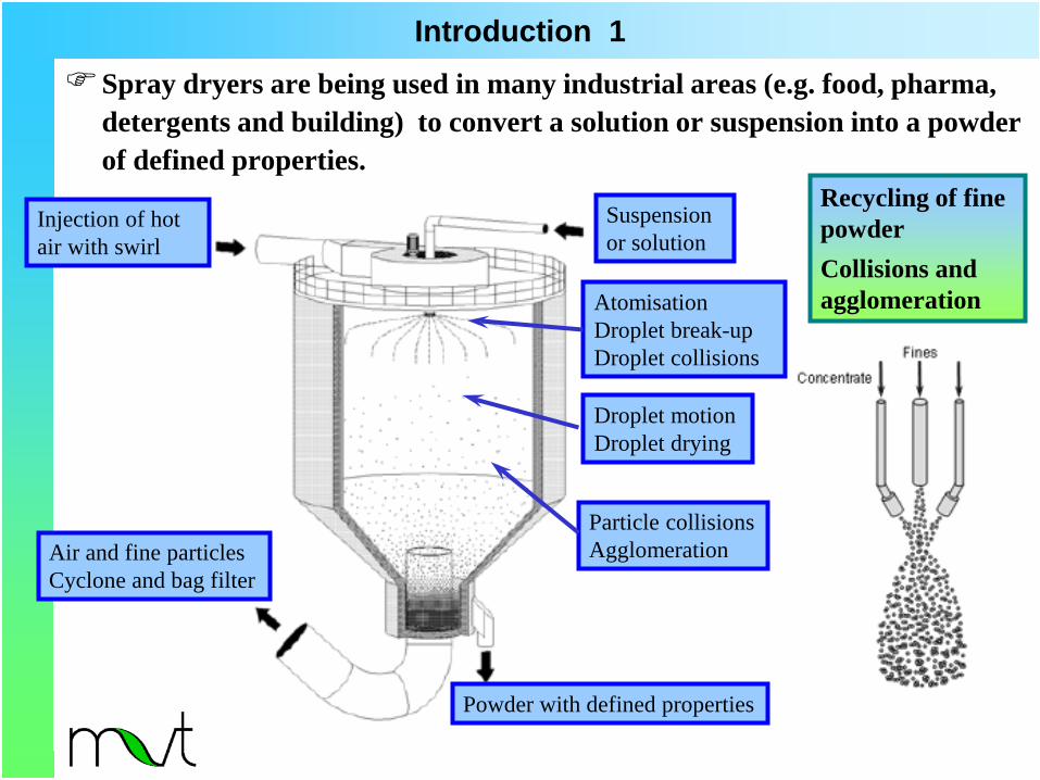
Introduction 1 Spray dryers are being used in many industrial areas (e.g. food, pharma,

detergents and building) to convert a solution or suspension into a powder of defined properties.

Recycling of fine powder Collisions and agglomeration

Injection of hot air with swirl

Suspension or solution

Atomisation Droplet break-up Droplet collisions

Droplet motion Droplet drying

Particle collisions Agglomeration Air and fine particles

Cyclone and bag filter

Powder with defined properties


Introduction 2 A spray dryer is used for converting a solution or

suspension into solid powder for further processing, transportation or commercial use.

Quite often the main target is producing a powder of desired properties which has certain properties (particle design).

Up to now the design of spray dryers and the determination of the operational conditions are based on a try-and-error approach in pilot-scale experiments.

This procedure is however not very satisfactory since it is time consuming and rather costly.

Since about 20 years, however, numerical approaches based on CFD (computational fluid dynamics) are increasingly applied for dryer design and optimization.

Due to the importance of particle size distribution the Euler/Lagrange approach is beneficial for such simulations.

A thorough computational tool is however not existing due to the numerous elementary processes influencing powder production in a spray dryer.

Brochure GEA Niro Spray Dryers

Fletcher et al. Applied Mathematical Modelling 30 (2006) 1281–1292


Introduction 3

Advantages of the Euler- Lagrange approach for spray dryer applications. Descriptive modelling of elementary

processes Consideration of droplet/particle size

distribution

Fluid Flow Simulation Particle Phase Simulation Two-Way Coupling

Grid generation URANS (unsteady Reynolds-

averaged conservation equations) • Effect of particles on flow

and turbulence LES (large-eddy simulations) • Modification of sub-grid-

scale turbulence Gas phase properties

(Vel, P, T, Species, ρ, µ)

Atomisation model (droplet injection) Simple blob model Spatially resolved droplet size and velocity measurements

Secondary break-up of droplets Wave, Rayleigh-Taylor, TAB, ETAB/CAB (Tanner 2004) Comparison by Kumzerova et al (2007)

Droplet tracking Relevant fluid forces (i.e. drag, lift, particle shape) Turbulence effect (isotropic, anisotropic turbulence)

Droplet drying Change of solids content and droplet properties

(µ and σ) Turbulence effects (instantaneous temperature field seen by the droplets)

Droplet collisions Bouncing Coalescence Separation (formation of satellite droplets)

Collisions of partially dried particles Partial or full penetration Modelling of agglomerate structure

Droplet/particle wall collisions Deposition or rebound collision (wall contamination)


Euler/Lagrange Approach 1 The fluid flow is calculated by solving the Reynolds-averaged conservation

equations by accounting for two-way coupling (source terms).

Turbulence model:

Conservation equations for: φ = 1, u, v, w, k, ε, Y, T k-ε turbulence model

Particle properties and Source Terms result from ensemble averaging

( ) ( ) ( ) ev,p,m,p, SSSzzyyxx

wz

vy

ux φφφ ++=

∂φ∂

Γ∂∂

−

∂φ∂

Γ∂∂

−

∂φ∂

Γ∂∂

−φρ∂∂

+φρ∂∂

+φρ∂∂

Two-way coupling procedure with under-relaxation

The Lagrangian approach relies on the tracking of a large number of representative point-particles (parcels) through the flow field accounting for all relevant forces like:

+ models for small- scale phenomena drag force gravity/buoyancy slip/shear lift slip/rotation lift torque on the particle

In-house code FASTEST/Lag-3D


Euler/Lagrange Approach 2

Dispersed phase (particles):

The instantaneous fluid velocity is generated by a single-step Langevin model.

( ) ( )( )

( )i

PiP

PFPFLR

2p

F

FpFPLS2p

FPi,PiDP

PP

i,PP

F1gmuuuuCD42

uuDCD42

uuuuCmD4

3td

udm

+

ρρ

−+Ω−×Ω

−πρ

+

ω×−πρ

+−−ρρ

=

Depending on the nature of the dispersed phase and the density ratio different relevant forces have to be used.

drag force gravity/ buoyancy slip-shear lift other forces, e.g. electrostatic slip-rotation lift

Ω⋅Ω

ρ=

ω

R

5pFp

p C2

D2dt

dI

Rotation:

pp u

dtxd

=

( ) ( ) i2

i,Pif

n,ii,Pf

1n,i r,tR1ur,tRu ξ∆∆−σ+∆∆=+


Lecture Content

New droplet drying model

with validation for a spray dryer


Droplet Drying Model 1

droplet suspended particles

Crust and enclosures

Drying stages of a spherical solution or suspension droplet

Two possible paths of droplet drying

B-C constant rate period

falling rate period

Wet-bulb temperature

t = 0 s t = 400 s t = 1800 s


Droplet Drying Model 2 A Mechanistic model is used to describe the four stages of

droplet drying (Darvan & Sommerfeld, IDS 2014) Stage A-B, initial heat-up period (sensible heating) TS equilibrium temperature (wet bulb temperature) Temperature distribution inside the droplet:

∂∂⋅

∂∂

⋅α

rT

rrr =

tdTd 2

2

( ) Rr:atTThrTk

0r:at0 rT

s =−=∂∂

−

==∂∂

∞

α: droplet thermal diffusivity k: thermal conductivity h: air heat transfer coefficient



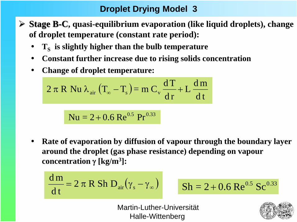
Stage B-C, quasi-equilibrium evaporation (like liquid droplets), change of droplet temperature (constant rate period): TS is slightly higher than the bulb temperature Constant further increase due to rising solids concentration Change of droplet temperature:

Rate of evaporation by diffusion of vapour through the boundary layer around the droplet (gas phase resistance) depending on vapour concentration γ [kg/m3]:

( )tdmdL

rdTdCm=TTNuR2 vsair +−λπ ∞

( )∞γ−γπ= sairDShR2tdmd

33.05.0 PrRe6.02=Nu +

33.05.0 ScRe6.02=Sh +



Stage C-D, crust formation and boiling (falling rate period): • Surface concentration CS reaches the saturation Csat • Crust formation due to crystallisation • droplet shrinkage is stopped • Two regions: dry outer crust and inner wet core

(fully saturated) • Discretisation of core and crust region • Interface tracking • Calculation of temperature distribution (crust and core region)

∂∂⋅

∂∂

⋅α

+∂∂

rT

rrr

rT

tdRd

Rr=

tdTd 2

2int

int

( )

intwb

s

Rr:atTT

Rr:atTThrTk

0r:at0 rT

==

=−=∂∂

−

==∂∂

∞α: droplet thermal diffusivity k: thermal conductivity h: air heat transfer coefficient


Droplet Drying Model 5 The heat balance at the interface (Rint) is used to track the interface in time

(depending on thermal conductivity of crust and core):

Vapour diffusion through boundary layer around liquid core and through the crust:

Solids concentration distribution within the droplet (diffusion):

( )

∂∂

−

∂∂

−=ρω−ω == int,Rrcoreint,Rrcrustint

avb0 rTk

rTk

tdRdL

( )

( )δ−δ

+

γ−γπ= ∞

cricricrustaircri

s

RRD2DShR1

2dtdm

∂∂

∂∂

=∂∂

rCDr

rr1

rC

AB2

2 ( )( )

−

∆−

ω+ω+

=3031

T1

RH

8.15139.323912.38DA

AAB

Internal diffusion of solids for skimmed milk

ωA: moisture content droplet ∆H: activation energy diffusion


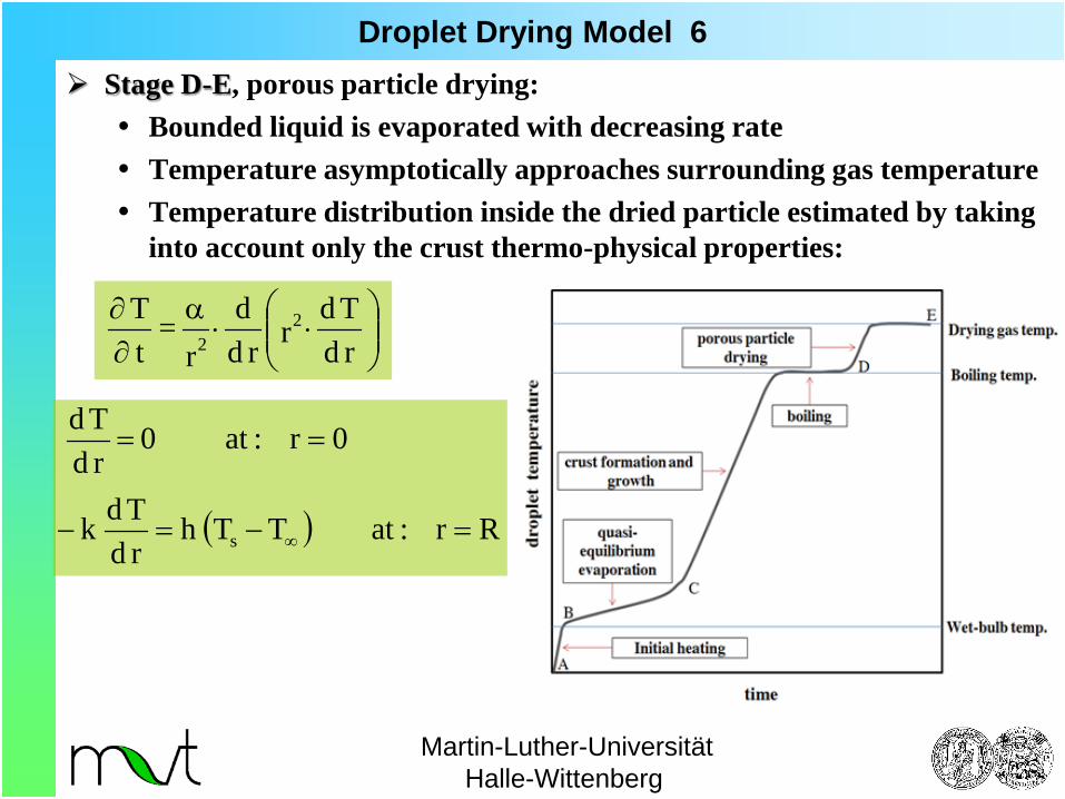
Droplet Drying Model 6 Stage D-E, porous particle drying: Bounded liquid is evaporated with decreasing rate Temperature asymptotically approaches surrounding gas temperature Temperature distribution inside the dried particle estimated by taking

into account only the crust thermo-physical properties:

⋅⋅

α∂∂

rdTd

rrdd

r =

tT 2

2

( ) Rr:atTThrdTdk

0r:at0 rdTd

s =−=−

==

∞


Droplet Drying Model 7 Comparison of the new drying model with experiments and „classical models“

0 50 100 150 200 250 300280

290

300

310

320

330

340

350

Experiment new model Farid model Nesic model Sano model

Tem

pera

ture

[K]

Time [s]

0 50 100 150 200 250 300

1x10-6

2x10-6

3x10-6

4x10-6 Experiment new model Farid model Nesic model Sano model

Mas

s [k

g]

Time [s]

Experiments for skim milk (solids 20% mass) by Chen et al. (1999): Vair = 1.0 m/s Tair = 343 K Tdrop,0 = 282 K D0 = 1.9 mm


Droplet Drying Model 8 Comparison of the new drying model with experiments:

0 10 20 30 40 50 60280300320340360380400420440460

Tem

pera

ture

[K]

Time [s]

1x10-6

2x10-6

3x10-6

4x10-6

5x10-6

Mas

s [k

g]

Colloidal silica, 30 % mass (Nesic & Vodnik 1991) Vair = 1.4 m/s Tair = 451 K Tdrop,0 = 293 K D0 = 2 mm

Sodium sulphate in water, 14 % mass (Nesic & Vodnik 1991) Vair = 1.0 m/s Tair = 383 K Tdrop,0 = 297 K D0 = 1.85 mm 0 50 100 150

280

300

320

340

360

380

Tem

pera

ture

[K]

Time [s]

0

1x10-6

2x10-6

3x10-6

Mas

s [k

g]


Droplet Drying Model 9 Radial distribution of mass and temperature within the droplet

0.0 0.2 0.4 0.6 0.8 1.00.35

0.40

0.45

0.50

0.55

0.60

0.65

t = 20 s t = 40 s t = 60 s

Mas

s [k

g solid /k

g tota

l]

R / R0 [ - ]

0.0 0.2 0.4 0.6 0.8 1.0310315

350

360

370

380

390

400

R / R0 [ - ]

t = 20 s t = 40 s t = 60 s

Tem

pera

ture

[K]

Experiments for skim milk (solids 30% mass) by Sano & Keey (1985) Vair = 1.0 m/s Tair = 423 K Tdrop,0 = 301 K D0 = 1.9 mm

0 20 40 60 80 100 120 140250

300

350

400

450

Tem

pera

ture

[K]

Time [s] 14:50


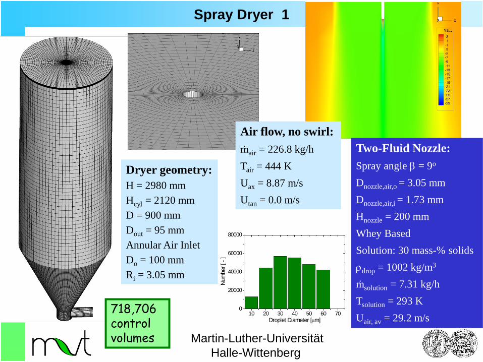
Spray Dryer 1

Dryer geometry: H = 2980 mm Hcyl = 2120 mm D = 900 mm Dout = 95 mm Annular Air Inlet Do = 100 mm Ri = 3.05 mm

Two-Fluid Nozzle: Spray angle β = 9o

Dnozzle,air,o = 3.05 mm Dnozzle,air,i = 1.73 mm Hnozzle = 200 mm Whey Based Solution: 30 mass-% solids ρdrop = 1002 kg/m3

ṁsolution = 7.31 kg/h Tsolution = 293 K Uair, av = 29.2 m/s

Air flow, no swirl: ṁair = 226.8 kg/h Tair = 444 K Uax = 8.87 m/s Utan = 0.0 m/s

10 20 30 40 50 60 700

20000

40000

60000

80000

Num

ber [

- ]

Droplet Diameter [µm]718,706 control volumes


Spray Dryer 2 Comparison of present calculations with results obtained with Fluent

0.0 0.1 0.2 0.3 0.4-10123456789

Particle Diameter 30 µm z = 0.4 m z = 1.0 m z = 2.1 m

Drop

let V

eloc

ity [m

/s]

Radius [m]

0.0 0.1 0.2 0.3 0.4320

330

340

350

360

370

Particle Diameter 30 µm z = 0.4 m z = 1.0 m z = 2.1 m

Drop

let T

empe

ratu

re [K

]

Radius [m]


Lecture Content

Droplet and particle collisions in spray dryer

stochastic inter-particle collision model experiments for viscous droplets


Inter-Particle Collisions in Spray Dryers Properties of droplets injected into a spray dryer (i.e. viscosity and surface tension) are strongly changing along their way through the dryer caused by drying of solution and suspension droplets (increasing solids content).

Surface tension dominated droplets Vicinity of atomiser

Viscosity dominated droplets Middle region of dryer

Droplets and solid particles Penetration Agglomerate formation Particle coating

Solid particles (low moisture content) Agglomeration van der Waals forces

Collisions of droplets/particles with different drying state


Stochastic Inter-Particle Collision Model 1 Stochastic Inter-Particle Collision Model (Sommerfeld 2001) In the trajectory calculation of the considered particle a fictitious collision

partner is generated for each time step. The properties of the fictitious particle are sampled from local distribution functions and correlations with the particle size.

In sampling the fictitious particle velocity fluctuation the correlation of the fluctuating velocity is respected (LES of Simonin):

Calculation of collision probability between the considered particle and the fictitious particle:

A collision occurs when a random number in the range [0 - 1] becomes smaller than the collision probability.

particle diameter particle velocities particle temperature solids content

( ) ( ) n2

LPii,realLPi,fict T,R1uT,Ru ξτ−σ+′τ=′ ( )

τ−=τ

4.0

L

pLp T

55.0expT,R

( ) tnuuDD4

tfP P2P1P2

2P1Pc ∆−+π

=∆=


Stochastic Inter-Particle Collision Model 2 The collision process is calculated in a co-ordinate system where the fictitious

particle is stationary.

Consideration of impact probability (small and large particles):

( )Larcsin1L:withZYL 22

=φ≤+=

π<Ψ< 20

Boundary particle

Stream lines

Separated particle

dp

DK

collector

Yc La

U0

K

2p2p1pp

i D18duu

µ

−ρ=

Ψ

Ca YL ≤Collision occurs if:

L

1

2L

u rel

φ

collision cylinder

2

1

Ψ2

1

( )

b

i

i

2

PK

c

adDY2

+ΨΨ

=

+

=η


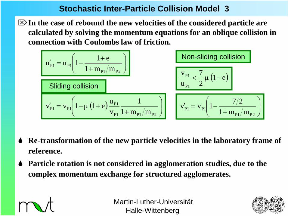
Stochastic Inter-Particle Collision Model 3 In the case of rebound the new velocities of the considered particle are

calculated by solving the momentum equations for an oblique collision in connection with Coulombs law of friction.

Re-transformation of the new particle velocities in the laboratory frame of reference.

Particle rotation is not considered in agglomeration studies, due to the complex momentum exchange for structured agglomerates.

+

+−=′

2P1P1P1P mm1

e11uu

Sliding collision

Non-sliding collision

( )

+

+µ−=′2P1P1P

1P1P1P mm1

1vue11vv

( )e127

uv

1P

1P −µ<

+

−=′2P1P

1P1P mm1271vv


Droplet Collision Modelling 1 The outcome of a droplet collision depends on numerous parameters, namely,

the kinetic properties and the thermo-physical properties of gas and droplets.

Governing non-dimensional parameters for the collision process:

The different collision scenarios are generally summarised in a phase diagram, i.e. B = f (WeC) Due to the large number of relevant properties a unique solution for the

collision regimes was not introduced so far !!!

Droplet velocities Droplet diameter ratio Impact angle

Droplet liquid (density and viscosity) Surface tension Type of gas phase Gas phase pressure and temperature

LS DDb2B+

=l

2relSl

CUDWe

σρ

=

( )Barcsin=φ

L

S

DD

=∆

Sll

lC D

Ohσρµ

=L

1

2b

u rel

φ

collision cylinder

2

1S: small L: large


Droplet Collision Modelling 2 Determination of the outcome of droplet collision based on B = f(We)

0 20 40 60 80 100 1200.0

0.2

0.4

0.6

0.8

1.0

reflexive separation

coalescence

bouncing

stretching separation

B [ -

]

We [ - ]

Calculation of post-collision droplet sizes and velocities

Not universally applicable → experiments to generalise the effect of viscosity

substances (PVP K30, K17, Saccharose, series of alcohols, FVA 1 reference oil

Relative velocity


Water for Validation

Images for We ∼ 30

σ

ρσµ

+=2

1

l

dl

l

lb21

d

a DC1We

CB

Ca =2.33 and Cb=0.41

Kuschel & Sommerfeld Exp. in Fluids, 2013


PVP K30 – 25 Ma%

PVP K30: 25 Ma%, η = 60.0 mP s Images for We ∼ 30

The oscillation of the droplets after coalescence is reduced with increasing dynamic viscosity

Ca =2.3378 and Cb =0.24


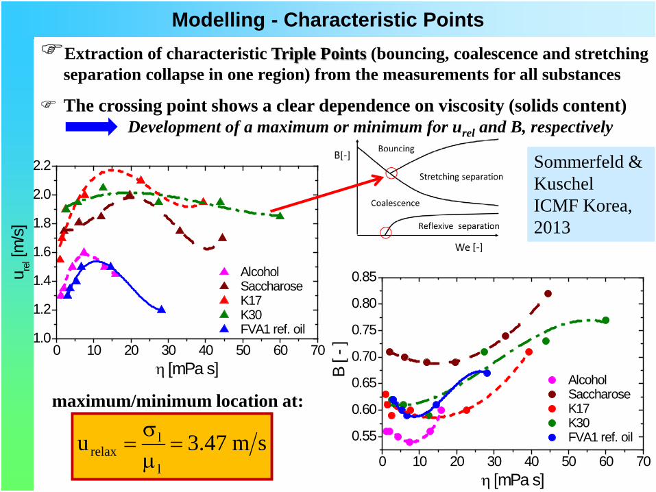
Modelling - Characteristic Points Extraction of characteristic Triple Points (bouncing, coalescence and stretching

separation collapse in one region) from the measurements for all substances

The crossing point shows a clear dependence on viscosity (solids content) Development of a maximum or minimum for urel and B, respectively

0 10 20 30 40 50 60 70

0.55

0.60

0.65

0.70

0.75

0.80

0.85

Alcohol Saccharose K17 K30 FVA1 ref. oil

η [mPa s]

B [ -

]0 10 20 30 40 50 60 701.0

1.2

1.4

1.6

1.8

2.0

2.2

Alcohol Saccharose K17 K30 FVA1 ref. oil

u rel [m

/s]

η [mPa s]

maximum/minimum location at:

sm47.3ul

lrelax =

µσ

=

Sommerfeld & Kuschel ICMF Korea, 2013


Modelling Onset of Stretching Separation Summary of Triple Point location for all systems Onset of stretching separation:

2e

112

Ca2

KeR−−

=

*Naue, G. and Bärwolff, G.: „Transportprozesse in Fluiden“, Deutscher Verlag für Grundstoff-Industrie, Leipzig, 1992.

relax

relrel

l

l

uUUCa =

σµ

=

l

relSl UDReµ

ρ=

0.01 0.1 1 1010

100

1000

PVP K17

Re [

- ]

Ca [ - ]

PVP K30

Alcohols Saccharose

FVA 1 Oil

Correlation Water

Qian Tetradecane 1 atm N2 (1997)

K=6.9451*

Resulting from a theory on maximum of information entropy for competing processes, i.e. interaction of flow structures with the mean flow K3 = 335 We for bubble break-up K4 = 2326 critical Re for laminar- turbulent pipe flow

left

right

sliding of two fluid surfaces

CWe


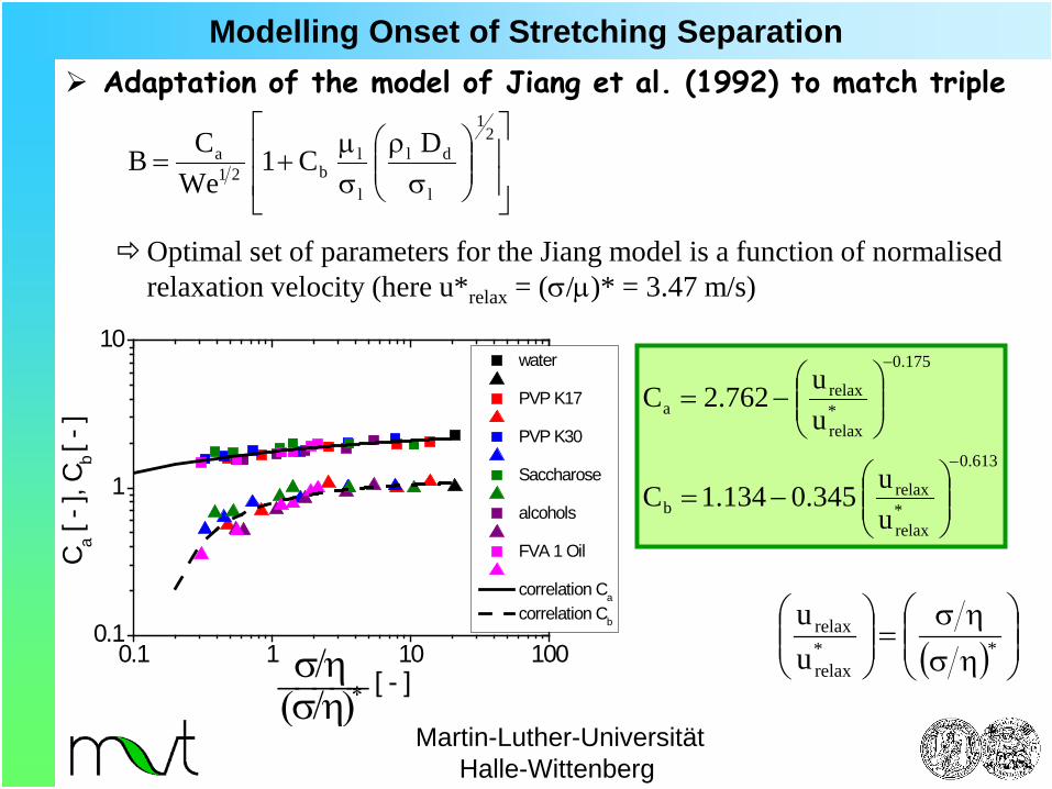
Modelling Onset of Stretching Separation Adaptation of the model of Jiang et al. (1992) to match triple

Optimal set of parameters for the Jiang model is a function of normalised

relaxation velocity (here u*relax = (σ/µ)* = 3.47 m/s)

σ

ρσµ

+=2

1

l

dl

l

lb21

a DC1We

CB

613.0

*relax

relaxb

175.0

*relax

relaxa

uu345.0134.1C

uu762.2C

−

−

−=

−=

0.1 1 10 1000.1

1

10 water PVP K17 PVP K30 Saccharose

alcohols FVA 1 Oil

correlation Ca

correlation Cb

[ - ]_____(σ/η)∗

C a [ -

], C b

[ - ]

σ/η ( )

ησησ

=

**

relax

relax

uu


Modelling - Onset of Reflexive Separation Critical We for the beginning of reflexive separation (at B = 0)

A correlation for all data can be found for We = f(Ca):

Modifying the model of Ashgriz and Poo to match critical Wecrit:

K2Ca3

KeW3

+=

( ) ( ) ( )LS

6

2323

23crit

114173WeWeη+η∆

∆+∆

∆+−∆++=

K=6.9451

0.01 0.1 1 10 10010

100

1000 Alcohols

We

[ - ]

Ca [ - ]

K17 K30

Saccharose FVA1 Reference Oil

Willis 200 (Silicon oil)

own exp, Park 1970, Ashgriz 1990 (water)

Jiang 1992 (Alcane)

Gotaas 2007 (MEG, DEG)

Qian 1997 (Tetradecan) We = K3/3 Ca + 2K

Deformation of the droplets


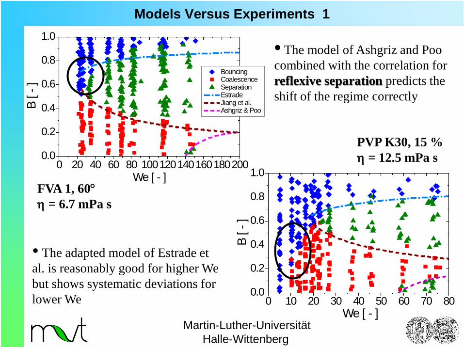
Models Versus Experiments 1

0 10 20 30 40 50 60 70 800.0

0.2

0.4

0.6

0.8

1.0

B [ -

]

We [ - ]

PVP K30, 15 % η = 12.5 mPa s 0 20 40 60 80 100120140160180200

0.0

0.2

0.4

0.6

0.8

1.0

Bouncing Coalescence Separation Estrade Jiang et al. Ashgriz & PooB

[ - ]

We [ - ]

• The model of Ashgriz and Poo combined with the correlation for reflexive separation predicts the shift of the regime correctly

• The adapted model of Estrade et al. is reasonably good for higher We but shows systematic deviations for lower We

FVA 1, 60° η = 6.7 mPa s


Models Versus Experiments 2

0 10 20 30 40 50 60 70 800.0

0.2

0.4

0.6

0.8

1.0

Bouncing Koaleszenz Separation Estrade Jiang

B [ -

]

We [ - ]Saccharose 60 % η = 57.3 mPa s

0 10 20 30 40 50 60 70 800.0

0.2

0.4

0.6

0.8

1.0

B [ -

]

We [ - ]

PVP K30, 25 % η = 60 mPa s

• For most of the substances the extended Jiang et al. model correctly predicts the boundary between coalescence and stretching separation

• Further studies are necessary for developing a general model for lower boundary of bouncing valid for the entire range of We


Lecture Content

New structure agglomeration model

with preliminary validation for a spray dryer

15:10


Agglomeration Model for Solid Particles

Agglomerate structure model

Location vectors Convex hull

Agglomeration models

Agglomerate structure Effective surface area Volume of convex hull Porosity of the agglomerate

Volume equivalent sphere

Simple agglomeration model

Number of primary particles

Penetration depth

Point-particle assumption

Hull

Part

VV1−=ε

Sequential agglomeration model

Number of primary particles Hull volume/diameter Porosity of hull Contact forces

Sommerfeld & Stübing ETMM 9, 2012


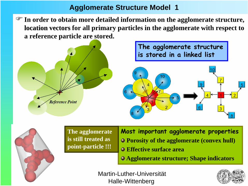
Agglomerate Structure Model 1 In order to obtain more detailed information on the agglomerate structure,

location vectors for all primary particles in the agglomerate with respect to a reference particle are stored.

Most important agglomerate properties Porosity of the agglomerate (convex hull) Effective surface area Agglomerate structure; Shape indicators

The agglomerate structure is stored in a linked list

The agglomerate is still treated as point-particle !!!


Agglomerate Structure Model 2 Assumptions for the stochastic collision model with respect to

structure modelling Agglomerates can only collide with primary particles (number concentration of the resulting agglomerates is very low). The fictitious particle cannot be an agglomerate, hence it is only sampled from the primary particle size distribution.

Extension of the stochastic collision model

The collision probability (based on a selected collision sphere of the agglomerate) predicts whether a collision occurs.

The collision process is calculated in a coordinate system where the agglomerate is stationary.

The point of impact on the surface of the selected collision sphere of the agglomerate is sampled stochastically

L


Agglomerate Structure Model 3 A collision occurs if the lateral displacement L is smaller than the boundary trajectory YC (impact efficiency). Random rotation of the agglomerate in all three directions (since rotation is neglected). The particle collides with the primary particle in the agglomerate being closest to the impact point (tracking). Possible collision scenarios:

L1

2

1

L1

2

1

sticking rebound Viscous particles: penetration


Penetration Model for High Viscous Droplets

Calculation of time-dependent penetration depth:

Radial: Tangential:

- Contact Area: - Penetration depth:

High viscous droplets penetrates into the low viscous droplet (spherical frame)

-ur

uϑ

uϕ

Ac

Motion of sphere in viscous liquid Shear force across contact area

Low viscosity

h

ϑϑ ⋅⋅µ−=⋅ ud

dtdum contLowHighrcontLow

rHigh ud3

dtdum ⋅⋅µ⋅π⋅−=⋅

rudtdr

=

2Lowcont hdh2d −⋅⋅=

r2

ddX LowHigh

P −+

=

0rforr2

dh

0rforXh

Low

P

≤−=

>=

ru

dtd ϑ=ϑ


Agglomeration Model for Solid Particles The occurrence of agglomeration may be decided on the basis of an energy

balance (dry particles only Van der Waals forces):

Critical impact velocity:

dvdw1k EEE +∆≤h

zo

R1

2a

R2

Van der Waals Energie:

Restitution ratio:

1k

d1k2pl E

EEk −=

∫∞

ππ

−=∆0z

23vdw dza

z6AE

( )ppl

20

2pl

2/12pl

1kr P6z

Akk1

R21U

ρπ

−=

Agglomeration if:

krrel UcosU

≤φ

( ) 1k2pld Ek1E −= Ho and Sommerfeld (2002)

R1: smaller particle


Geometry of the Spray Dryer 1 Geometry and operational conditions of spray dryer (NIRO Copenhagen):

Dryer geometry: H = 4096 mm Hcyl = 1960 mm D = 2700 mm Hout = 3303 mm Dout =210 mm Annular Air Inlet Ro = 527 mm Ri = 447 mm

Air flow with swirl: ṁair = 1900 kg/h φair = 1.1 mass-% Tair = 452.5 K Uax = 9.8 m/s Utan = 2.4 m/s

Pressure nozzle: Hollow cone nozzle pnozzle = 85 bar Spray angle β = 52o

Dnozzle = 2 mm Hnozzle = 270 mm Maltodextrine DE-18 Solution: 29 mass-% solids ρdrop = 1090 kg/m3

ṁsolution = 92 kg/h Tsolution = 293 K Uav = 127 m/s

Fines return: Annular inlet around the nozzle Do = 72 mm Di = 63 mm Ufine = 37 m/s ρfine = 440 kg/m³


Geometry of the Spray Dryer 2 Numerical discretisation and boundary conditions of the spray dryer:

Inlet and boundary conditions: Inlet: assumed velocity profiles Walls: no-slip velocity heat transfer coefficient ⇒ measurements h = 10.5 W/(K⋅m²), Outlet pipe: gradient free

Discretisation: 138 blocks 586.564 meshes

0 20 40 60 80 100 120 140 1600

2000400060008000

1000012000140001600018000

Num

ber [

- ]

Particle Diameter [µm]

Spray Droplets Fines Return

Droplet and Particle Sizes


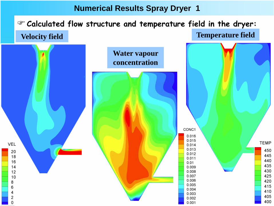
Numerical Results Spray Dryer 1

Calculated flow structure and temperature field in the dryer: Velocity field Temperature field

Water vapour concentration


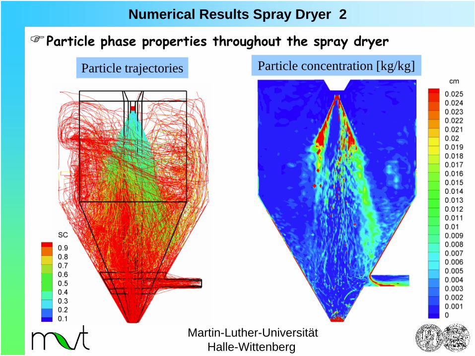
Numerical Results Spray Dryer 2

Particle phase properties throughout the spray dryer

Particle trajectories Particle concentration [kg/kg]


Numerical Results Spray Dryer 3 Particle-phase properties throughout the spray dryer

Solids content in the particles Local particle mean diameter


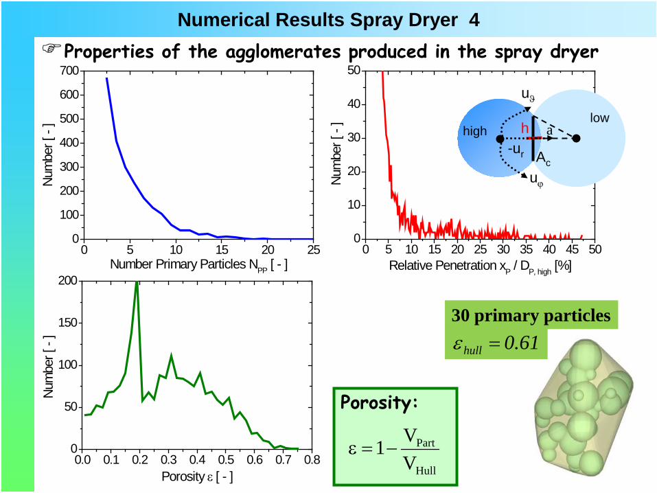
Numerical Results Spray Dryer 4 Properties of the agglomerates produced in the spray dryer

Porosity:

Hull

Part

VV1−=ε

0 5 10 15 20 250

100

200

300

400

500

600

700

Nu

mbe

r [ -

]

Number Primary Particles NPP [ - ]

0.0 0.1 0.2 0.3 0.4 0.5 0.6 0.7 0.80

50

100

150

200

Num

ber [

- ]

Porosity ε [ - ]

0 5 10 15 20 25 30 35 40 45 500

10

20

30

40

50

Num

ber [

- ]

Relative Penetration xP / DP, high [%]

-ur

uϑ

uϕ

Ac

high low

h a

61.0hull =ε30 primary particles


Numerical Results Spray Dryer 5 Simulated agglomerates compared with agglomerates collected from the spray dryer


Outlook 1 Sub-models for describing the behaviour of droplets and particles in a

spray dryer have been developed and validated; i.e. drying, viscous droplet collisions and agglomeration model.

The models will be jointly implemented in the in-house code FASTEST/Lag-3D and further validated.

Extension of the droplet collision model for very high viscosities; i.e. up to several Pa⋅s.

Feeding Liquid (up to 16bar)

Outlet

a

b c

d

Coalescence Separation Stretching


Outlook 2 Validation of the droplet collision models using a special laboratory spray dryer with interacting sprays.


Acknowledgements

The financial support of projects by the Deutsche Forschungsgemeinschaft (DFG) is gratefully acknowledged.

The following Ph.D. students have contributed to the presented research:

Dipl.-Ing. Stefan Blei

M.Sc. Ali Darvan

M.Sc. Chi-Ahn Ho

Dipl.-Ing. Matthias Kuschel

Dr.-Ing. Hai Li

Dipl.–Ing. Sebastian Stübing


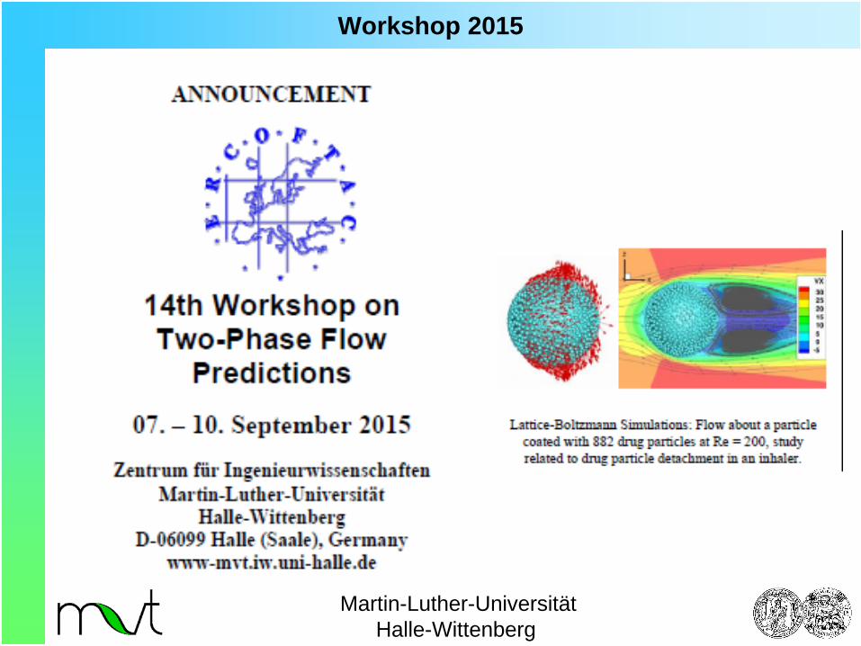
Workshop 2015

modelling requirements for cfd calculations of spray dyers

Documents